The Feature-First Block Model

Abstract

Labelled networks are an important class of data, naturally appearing in numerous applications in science and engineering. A typical inference goal is to determine how the vertex labels (or features) affect the network’s structure. In this work, we introduce a new generative model, the feature-first block model (FFBM), that facilitates the use of rich queries on labelled networks. We develop a Bayesian framework and devise a two-level Markov chain Monte Carlo approach to efficiently sample from the relevant posterior distribution of the FFBM parameters. This allows us to infer if and how the observed vertex-features affect macro-structure. We apply the proposed methods to a variety of network data to extract the most important features along which the vertices are partitioned. The main advantages of the proposed approach are that the whole feature-space is used automatically and that features can be rank-ordered implicitly according to impact.

1 Introduction

Many real-world networks exhibit strong community structure, with most nodes belonging to densely connected clusters. Finding ways to recover the latent communities from the observed graph is an important task in many applications, including compression [1] and link prediction [4]. In this work, we examine vertex-labelled networks, referring to the labels as features. A typical goal is to determine whether a given feature impacts graphical structure. Answering this requires a random graph model; the standard is the stochastic block model (SBM) [7]. Numerous variants of the SBM have been proposed, e.g., the MMSBM [2] and OSBM [14], but these do not include features in the graph generation process.

To analyse a labelled network using one of the simple SBM variants, a typical procedure would be to partition the graph into blocks grouped by distinct values of the feature of interest. The associated model can then be used to test for evidence of heterogeneous connectivity between the feature-grouped blocks. Nevertheless, this approach can only consider disjoint feature sets and the feature-grouped blocks are often an unnatural partition of the graph.

We would instead prefer to partition the graph into its most natural blocks and then find which of the available features – if any – best predict the resulting partition. Thus motivated, we present a novel framework for modelling labelled networks, which we call the feature-first block model (FFBM). This is an extension of the SBM to labelled networks.

2 Preliminaries

We first need a model for community-like structure in a network. For this we adopt the widely-used stochastic block model (SBM). This is a latent variable model where each vertex belongs to a single block and the probability two vertices are connected depends only on the block memberships of each. Specifically, we will use the microcanonical variant of the SBM, proposed by Peixoto [10]. To allow for degree-variability between members of the same block, we adopt the following degree-corrected formulation (DC-SBM):

Definition 1 (Microcanonical DC-SBM)

Let $N\geq 1$ denote the number of vertices in an undirected graph with $E$ edges. The block memberships are encoded by a vector $b\in[B]^{N}$, where $B$ is the number of non-empty blocks. Let $e=(e_{rs})$ be the $B\times B$ symmetric matrix of edge counts between blocks, such that $e_{rs}$ is the number of edges from block $r$ to block $s$. Let $k=(k_{i})$ denote a vector of length $N$, with $k_{i}$ being the degree of vertex $i$.

The graph’s adjacency matrix $A\in\{0,1\}^{N\times N}$ is generated by placing edges uniformly at random, conditional on the constraints imposed by $b$, $e$ and $k$ being satisfied. Specifically, if $A\sim\mbox{\rm DC-SBM}_{\rm MC}(b,e,k)$, then with probability 1 it satisfies, for all $r,s\in[B]$ and all $i\in[N]$:

$$e_{rs}=\sum_{i,j\in[N]}A_{ij}\mathbbm{1}\{b_{i}=r\}\mathbbm{1}\{b_{j}=s\}\qquad\textrm{and}\qquad k_{i}=\sum_{j\in[N]}A_{ij}.$$ (1)

3 Feature-First Block Model

In this section we propose a novel generative model for labelled networks. We call this the feature-first block model (FFBM), illustrated in Figure 1.

Let $N$ denote the number of vertices, $B$ the number of blocks and ${\cal X}$ the set of values each feature can take. We define the vector $x_{i}\in\mathcal{X}^{D}$ as the feature vector for vertex $i$, where $D$ is the number of features associated with each vertex. For example, in the datasets we analyse, we deal with binary feature flags (denoting the presence/absence of each feature), so $\mathcal{X}=\{0,1\}$. We write $X$ for the $N\times D$ feature matrix containing the feature vectors $\{x_{i}\}_{i=1}^{N}$ as its rows.

For the FFBM, we start with the feature matrix $X$ and generate a random vector of block memberships $b\in[B]^{N}$. For each vertex $i$, the block membership $b_{i}\in[B]$ is generated based on the feature vector $x_{i}$, independently between vertices. The conditional distribution of $b_{i}$ given $x_{i}$ also depends on a collection of weight vectors $\theta=\{w_{k}\}_{k=1}^{B}$, where each $w_{k}$ has dimension $D$. We will later find it convenient to write $\theta$ as a $B\times D$ matrix of weights $W$. Specifically, the distribution of $b$ given $X$ and $\theta$ is,

$$p(b|X,\theta)=\prod_{i\in[N]}p(b_{i}|x_{i},\theta)=\prod_{i\in[N]}\phi_{b_{i}}(x_{i};\theta)=\prod_{i\in[N]}\frac{\exp\left(w_{b_{i}}^{T}x_{i}\right)}{\sum_{k\in[B]}\exp\left(w_{k}^{T}x_{i}\right)}.$$ (2)

Note that $\phi_{b_{i}}$ has the form of a softmax activation function. More complex models based on different choices for the distributions $\phi_{b_{i}}$ above are also possible, but then deriving meaning from the inferred parameter distributions is more difficult.

Figure 1: The Feature-First Block Model (FFBM)

Once the block memberships $b$ have been generated, we then draw the graph $A$ from the microcanonical DC-SBM with additional parameters $\psi=\{\psi_{e},\psi_{k}\}$:

$$A\sim\textrm{DC-SBM}_{\textrm{MC}}(b,\psi_{e},\psi_{k}).$$ (3)

3.1 Prior selection

To complete the description of our Bayesian framework, priors on $\theta$ and $\psi$ must also be specified. We place a Gaussian prior on $\theta$ such that each element of $\theta$ has an independent ${\cal N}(0,\sigma_{\theta}^{2})$ prior, with hyperparameter $\sigma_{\theta}^{2}$:

$$p(\theta)\sim\mathcal{N}\left(\theta;0,\sigma_{\theta}^{2}I\right).$$ (4)

This choice of prior gives a very simple form for the conditional distribution of the block membership vector $b$ given $X$; it is a uniform distribution:

$$p(b|X)=\int p(b|X,\theta)p(\theta)d\theta=B^{-N}.$$ (5)

The proof is given in Appendix 0.A.1. This is an important simplification as evaluating $p(b|X)$ does not require an expensive integration over $\theta$ nor does it depend on $X$. Peixoto [10] proposes careful choices for the priors on the additional microcanonical SBM parameters $\psi$, which we adopt without repeating their exact form here. The idea is to write the joint distribution on $(b,e,k)$ as a product of conditionals, $p(b,e,k)=p(b)p(e|b)p(k|e,b)=p(b)p(\psi|b)$. In our case, conditioning on $X$ is also necessary, leading to, $p(b,\psi|X)=p(b|X)p(\psi|b,X)=p(b|X)p(\psi|b),$ where we used the fact $\psi$ and $X$ are conditionally independent given $b$. All that concerns the main argument is that $p(\psi|b)$ has an easily computable form.

4 Inference

Having completed the definition of the FFBM, we wish to leverage it to perform inference. Specifically, given a labelled network $(A,X)$, we wish to infer if and how the observed features $X$ impact the graphical structure $A$. Formally, this means characterising the posterior distribution: $p(\theta|A,X)\propto p(\theta)\cdot p(A|X,\theta).$ Although the prior is easily computable, computing the likelihood requires summing over all latent block-states, $p(A|X,\theta)=\sum_{b\in[B]^{N}}p(A|b)P(b|X,\theta)$, which is clearly impractical. In fact, this approach is doubly intractable as we would also need to compute the normalising constant $p(A|X)$. Therefore, following standard Bayesian practice, instead we aim to draw samples from the posterior,

$$\theta^{(t)}\sim p(\theta|A,X).$$ (6)

We propose an iterative Markov chain Monte Carlo (MCMC) approach to obtain these samples $\{\theta^{(t)}\}$. We first draw a sample $b^{(t)}$ from the block membership posterior, and then use $b^{(t)}$ to obtain a corresponding sample $\theta^{(t)}$:

$$b^{(t)}\stackrel{{\scriptstyle\rm distr}}{{\approx}}p\big{(}b|A,X\big{)}\quad\textrm{then}\quad\theta^{(t)}\stackrel{{\scriptstyle\rm distr}}{{\approx}}p\big{(}\theta|X,b^{(t)}\big{)},$$ (7)

where these approximations become exact as the number of MCMC iterations $t\to\infty$. As described in the following subsections, this can be implemented through a two-level Markov chain via the Metropolis-Hastings (MH) algorithm [5]. The splitting of the Markov chain into two levels allows us to side-step the summation over all latent $b\in[B]^{N}$ required to directly compute the likelihood, $p(A|X,\theta)$. The resulting $\theta^{(t)}$ samples are asymptotically unbiased in that the expectation of their distribution converges to the true posterior:

$$\lim_{t\to\infty}\mathbb{E}_{b^{(t)}}\left[p\left(\theta|X,b^{(t)}\right)\right]=\sum_{b\in[B]^{N}}p(\theta|X,b)p(b|A,X)=p(\theta|A,X).$$ (8)

This is an example of a pseudo-marginal approach; see, e.g., Andrieu and Roberts [3] for a detailed rigorous derivation based on (8).

Figure 2: $\theta$-sample generation.

Figure 2 shows an overview of the proposed method, with $q$ and $\alpha$ denoting the MH proposal distribution and acceptance probability respectively. Note the importance of the simplification in (5). As evaluating $p(b|X)$ does not depend on $X$, we do not need $X$ to sample $b$. And on the other level, in order to obtain samples for $\theta$ we use only $b$ but not $A$, as $(\theta\perp\!\!\!\perp A)|b$.

4.1 Sampling block memberships

To generate the required $b$-samples, we adopt the MCMC procedure of [9], which relies on writing the posterior in the following form,

$$p(b|A,X)\propto p(A|b,X)\cdot p(b|X)=\pi_{b}(b),$$ (9)

where $\pi_{b}(\cdot)$ denotes the un-normalised target density. Since we are using the microcanonical SBM formulation, there is only one value of $\psi$ that is compatible with the given $(A,b)$ pair; recall the constraints in (1). We denote this value $\psi^{*}=\{\psi_{k}^{*},\psi_{e}^{*}\}$. Therefore, the summation over all $\psi$ needed to evaluate $p(A|b,X)$ reduces to just the single $\psi^{*}$ term: $p(A|b,X)=\sum_{\psi}\nolimits p(A,\psi|b,X)=p(A,\psi^{*}|b,X)$. In this context, the microcanonical entropy of the configuration $b$ is,

$$S(b)\coloneqq-\log\pi_{b}(b)=-\Big{(}\log p(A|b,\psi^{*})+\log p(\psi^{*},b|X)\Big{)},$$ (10)

which can be thought of as the optimal “description length” of the graph. This expression will later be employed to help evaluate experimental results. The exact form of the proposal $q_{b}$ is explored thoroughly in [9] and not repeated here. We use the graph-tool [11] library for Python, which implements this algorithm. The only modification is in the prior $p(b)$ that we replace with $p(b|X)=B^{-N}$, which cancels out in the MH accept-reject step as it is independent of $b$.

4.2 Sampling feature-to-block generator parameters

The target distribution for the required $\theta$-samples is the posterior of $\theta$ given the values of the pair $(X,b)$. We write this as,

$$\pi_{\theta}(\theta)\propto p(\theta|X,b)\propto p(b|X,\theta)p(\theta)\propto\exp\left(-U(\theta)\right),$$ (11)

where $U(\theta)$ denotes the negative log-posterior. Let $y_{ij}\coloneqq\mathbbm{1}\left\{b_{i}=j\right\}$ and $a_{ij}\coloneqq\phi_{j}(x_{i};\theta)$. Discarding constant terms, $U(\theta)$ can be expressed as,

$$U(\theta)=\left(\sum_{i\in[N]}\sum_{j\in[B]}y_{ij}\log\frac{1}{a_{ij}}\right)+\frac{1}{2\sigma_{\theta}^{2}}\|\theta\|^{2}=N\cdot\mathcal{L}(\theta)+\frac{1}{2\sigma_{\theta}^{2}}\|\theta\|^{2};$$ (12)

see Appendix 0.A.2. The function $U(\theta)$ is a typical objective function for neural network training. The first term $N\cdot\mathcal{L}(\theta)$ is introduced by the likelihood and represents the cross-entropy between the graph-predicted and feature-predicted block memberships. The second term, introduced by the prior, brings a form of regularisation, guarding against over-fitting. In order to draw samples from the posterior $\pi_{\theta}\propto\exp(-U)$ we adopt the Metropolis-adjusted Langevin algorithm (MALA) [12], which uses $\nabla U$ to bias the proposal towards regions of higher density. Given the current sample $\theta$, a proposed new sample $\theta^{\prime}$ is generated from,

$$\theta^{\prime}\sim q_{\theta}\big{(}\theta,\theta^{\prime}\big{)}=\mathcal{N}\big{(}\theta^{\prime};\theta-h\nabla U(\theta),2hI\big{)},$$

where $\xi\sim\mathcal{N}(0,I)$ and $h$ is a step-size parameter which may vary with the sample index. Without the injected noise term $\xi$, MALA is equivalent to gradient descent. We require $\xi$ to fully explore the parameter space. The term $\nabla U$ has an easy to compute analytic form (derived in Appendix 0.A.2).

4.3 Sampling sequence

So far, each $\theta^{(t)}$ update has used its corresponding $b^{(t)}$ sample. This means the evaluation of $U^{(t)}$ and $\nabla U^{(t)}$ has high variance, leading to longer burn-in and possibly slower MCMC convergence. The only link between $b^{(t)}$ and $\theta^{(t)}$ is in the evaluation of $U^{(t)}$ and $\nabla U^{(t)}$ which depends only on the matrix $y^{(t)}$ with entries $y_{ij}^{(t)}\coloneqq\mathbbm{1}\{b_{i}^{(t)}=j\}$. We would rather deal with the expectation of each $y_{ij}^{(t)}$:

$$\mathbb{E}\left[y_{ij}^{(t)}\right]=\mathbb{E}_{b^{(t)}}\left[\mathbbm{1}\left(b_{i}^{(t)}=j\right)\right]=p(b_{i}=j|A,X).$$ (13)

An unbiased estimate for this can be obtained using the thinned $b$-samples after burn-in. Let $\mathcal{T}_{b}$ denote the retained set of indices for the $b$-samples and $\mathcal{T}_{\theta}$ similarly for the $\theta$-chain. The unbiased estimate for $y_{ij}^{(t)}$ is then:

$$\hat{y}_{ij}\coloneqq\frac{1}{|\mathcal{T}_{b}|}\sum_{t\in\mathcal{T}_{b}}y_{ij}^{(t)}=\frac{1}{|\mathcal{T}_{b}|}\sum_{t\in\mathcal{T}_{b}}\mathbbm{1}\{b_{i}^{(t)}=j\}.$$ (14)

The same matrix $\hat{y}$ is used in each $\theta^{(t)}$ update step. This way, it is not necessary to run the $b$ and $\theta$ Markov chains concurrently. Instead, we run the $b$-chain to completion and use it to generate $\hat{y}$ also allowing us to vary the lengths of each.

4.4 Dimensionality reduction

The complexity of evaluating $U$ and $\nabla U$ is linear in the dimension of the feature space $D$, so there is computational incentive to reduce $D$. Given the samples $\left\{\theta^{(t)}\right\}$, we can compute the empirical mean and standard deviation of each component of $\theta$. Switching to the matrix notation $W$ for $\theta$, let:

$$\hat{\mu}_{ij}\coloneqq\frac{1}{|\mathcal{T}_{\theta}|}\sum_{t\in\mathcal{T}_{\theta}}W_{ij}^{(t)}\qquad\textrm{and}\qquad\hat{\sigma}_{ij}^{2}\coloneqq\frac{1}{|\mathcal{T}_{\theta}|}\sum_{t\in\mathcal{T}_{\theta}}\left(W_{ij}^{(t)}-\hat{\mu}_{ij}\right)^{2}.$$ (15)

A simple heuristic to discard the least important features requires specifying a cutoff $c>0$ and a multiplier $k>0$. We define the function $\mathcal{F}_{i}(j)$ as in (16) and only keep features with indices $d\in\mathcal{D}^{\prime}$, where $\mathcal{D}^{\prime}$ is given in (17).

$$\mathcal{F}_{i}(j) \coloneqq(\hat{\mu}_{ij}-k\hat{\sigma}_{ij},\hat{\mu}_{ij}+k\hat{\sigma}_{ij})\cap(-c,+c),$$ (16)

$$\mathcal{D}^{\prime} \coloneqq\left\{j\in[D]:\exists i\in[B]\textrm{ s.t. }\mathcal{F}_{i}(j)=\emptyset\right\}.$$ (17)

Intuitively, this means discarding any feature $j$ for which $(\hat{\mu}_{ij}-k\hat{\sigma}_{ij},\hat{\mu}_{ij}+k\hat{\sigma}_{ij})$ overlaps with $(-c,c)$ for all $i$. If we were to use the Laplace approximation for the posterior $p(W_{ij}|A,X)\approx\mathcal{N}(W_{ij};\hat{\mu}_{ij},\hat{\sigma}_{ij}^{2})$, then this would be analogous to a hypothesis test on the magnitude of $W_{ij}$ compared to $c$ with multiplier $k$ in (16) determining the degree of significance of the result. Conversely, if we want to fix the number of dimensions in our reduced feature set $|\mathcal{D}^{\prime}|=D^{\prime}$, the problem then becomes finding the largest value of $c$ such that $|\mathcal{D}^{\prime}|=D^{\prime}$ given $k=k_{0}$:

$$c^{*}=\operatorname*{arg\,max}\{c>0\;:\;|\mathcal{D}^{\prime}|=D^{\prime},k=k_{0}\}.$$ (18)

5 Experimental results

We apply our proposed methods to a variety of labelled networks:

• Political books [8] ($N=105,E=441,D=3$) – network of Amazon political books published close to the 2004 presidential election. Two books are connected if they were frequently co-purchased. Vertex features encode the political affiliation of the author (liberal, conservative, or neutral).

• Primary school dynamic contacts [13] ($N=238,E=5539,D=13$) – network of 238 individuals (students and teachers), with edges denoting face-to-face contacts at a primary school in Lyon, France. The vertex features are class membership (one of 10 values: 1A-5B), gender (male, female), and status (teacher, student). We choose to analyse just the second day of results.

• Facebook egonet [6] ($N=747,E=30025,D=480$) – network of Facebook users with edges denoting “friends”. Vertex features are fully anonymised and encode information about each user’s education history, languages spoken, gender, home-town, birthday etc. We focus on the egonet with id 1912.

For reference, the inferred partitions for all of these are given on Figure 3. We employ the following metrics to assess model performance. First, the average description length per entity (nodes and edges) $\bar{S}_{e}$ used to gauge the SBM fit is defined as:

$$\bar{S}_{e}\coloneqq\frac{1}{(N+E)|\mathcal{T}_{b}|}\sum_{t\in\mathcal{T}_{b}}S\left(b^{(t)}\right).$$ (19)

Next, to assess the performance of the feature-to-block predictor, the vertex set $[N]$ is partitioned at random so that a constant fraction $f$ of vertices form the training set $\mathcal{G}_{0}$ and the remainder form the test set $\mathcal{G}_{1}$. The $b$-chain is run using the whole network but only vertices $v\in\mathcal{G}_{0}$ are used for the $\theta$-chain. Then the the average cross-entropy loss over each set is used to gauge the quality of the fit,

$$\bar{\mathcal{L}}_{\star}\coloneqq\frac{1}{|\mathcal{T}_{\theta}|}\sum_{t\in\mathcal{T}_{\theta}}\mathcal{L}_{\star}^{(t)},\quad\textrm{where}\quad\mathcal{L}_{\star}^{(t)}\coloneqq\frac{1}{|\mathcal{G}_{\star}|}\sum_{i\in\mathcal{G}_{\star}}\sum_{j\in[B]}\hat{y}_{ij}\log\frac{1}{\phi_{j}\left(x_{i};\theta^{(t)}\right)},$$ (20)

where $\star\in\{0,1\}$ toggles between the training and test sets and $\hat{y}_{ij}$ is defined in (14). Nevertheless, the cross-entropy loss is a coarse measure of fit. A new measure, specific to each detected block, can be defined as follows. Let $\mathcal{B}_{\star}(j)$ be the set of vertices with maximum a posteriori probability of belonging to block $j$, $\mathcal{B}_{\star}(j)\coloneqq\{i\in\mathcal{G}_{\star}:\hat{b}_{i}=j\},$ where $\hat{b}_{i}\coloneqq\operatorname*{arg\,max}_{j}\hat{y}_{ij},$ and define the block-accuracy for block $j$ as,

$$\eta_{\star}(j)\coloneqq\frac{1}{|\mathcal{B}_{\star}(j)|\cdot|\mathcal{T}_{\theta}|}\sum_{i\in\mathcal{B}_{\star}(j)}\sum_{t\in\mathcal{T}_{\theta}}\mathbbm{1}\left\{\hat{b}_{i}=\operatorname*{arg\,max}_{j}\phi_{j}\left(x_{i};\theta^{(t)}\right)\right\}.$$ (21)

This effectively tests whether the feature-to-block and graph-to-block predictions agree in their largest component. For the higher-dimensional datasets, we also apply the dimensionality reduction method of Section 4.4. We then retrain the feature-block predictor using only the retained feature set $\mathcal{D}^{\prime}$, and report the log-loss over the training and test sets for the reduced classifier – denoted $\bar{\mathcal{L}}_{0}^{\prime}$ and $\bar{\mathcal{L}}_{1}^{\prime}$ respectively.

(a) Polbooks

(b) Primary school

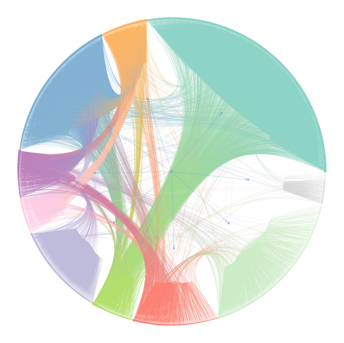
(c) Facebook egonet

(d) Block Legend

Figure 3: Networks laid out and coloured according to inferred block memberships for a given experiment iteration. Visualisation performed using graph-tool [11].

Table 1: Experimental results averaged over $n=10$ iterations (mean $\pm$ std. dev.).

Dataset	$B$	$D$	$D^{\prime}$	$\bar{S}_{e}$	$\bar{\mathcal{L}}_{0}$	$\bar{\mathcal{L}}_{1}$	$c^{*}$	$\bar{\mathcal{L}}_{0}^{\prime}$	$\bar{\mathcal{L}}_{1}^{\prime}$
Polbooks	3	3	–	$2.250\pm 0.000$	$0.563\pm 0.042$	$0.595\pm 0.089$	–	–	–
School	10	13	10	$1.894\pm 0.004$	$0.787\pm 0.127$	$0.885\pm 0.129$	$1.198\pm 0.249$	$0.793\pm 0.132$	$0.853\pm 0.132$
FB egonet	10	480	10	$1.626\pm 0.003$	$1.326\pm 0.043$	$1.538\pm 0.069$	$0.94\pm 0.019$	$1.580\pm 0.150$	$1.605\pm 0.106$

(a) Political books

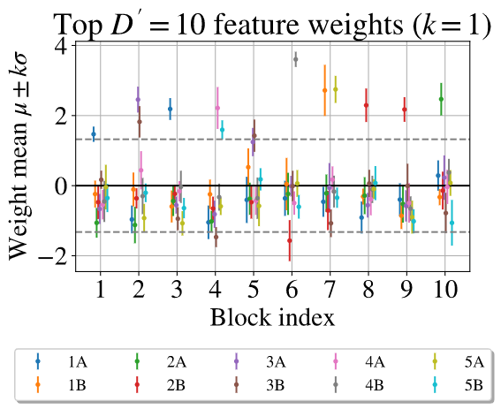
(b) Primary school

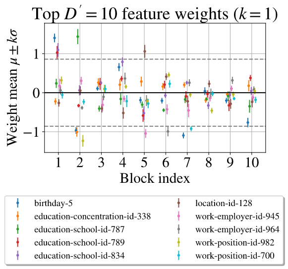
(c) Facebook egonet

Figure 4: Top $D^{\prime}$ $\theta$-samples for each dataset. Coarse steps on x-axis give block index and the fine steps denote give index. Dotted line is $\pm c^{*}$.

(a) Political books

(b) Primary school

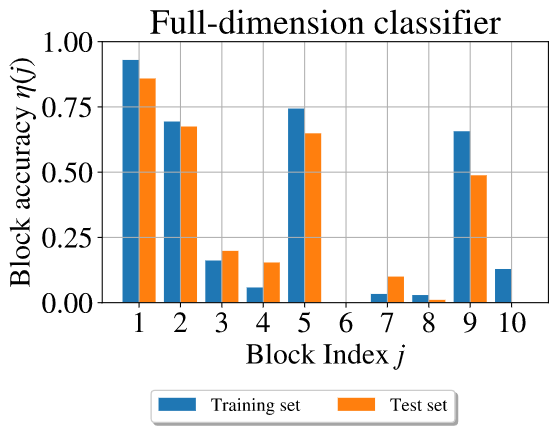
(c) Facebook egonet

Figure 5: Per-block accuracy $\eta(j)$ for each dataset.

Table 1 summarises the results for each experiment. We see that the dimensionality reduction procedure brings the training and test losses closer. This indicates that the retained features are indeed well correlated with the underlying graphical partition and that the approach generalises correctly. The test loss variance is higher than the training loss variance as the test set is smaller and so more susceptible to variability in its construction. The average description length per entity of the graph, $\bar{S}_{e}$, has very small variance, suggesting that the detected communities can be found reliably (to within an arbitrary relabelling of blocks).

Political books.

We choose to partition the network into $B=3$ communities as we only have this many distinct values for political affiliation. From Figure 4(a) we see that all 3 blocks have a distinct political affiliation as their largest positive component. Furthermore, the training and test losses from Table 1 are very similar and both are low in magnitude. This is strong evidence that political affiliation is a very appropriate explanatory variable for the overall network structure. However, from Figure 5(a) we see that block 1 has low accuracy. This suggests that detected block 1 is not solely composed of “neutral” books but also contains some “liberal” and “conservative” authors. Examining Figure 3(a), we see the majority of paths between blocks 2 and 3 go through block 1. Block 1 is in effect a bridge between the “conservative” and “liberal” blocks so it is unsurprising that some of these leak into block 1.

Primary school.

We choose the number of communities $B=10$, in line with the total number of school classes. Only the pupils’ class memberships (1A-5B) survive the dimensionality-reduction process (Figure 4(b)); gender and teacher/student status have been discarded, meaning these are poor predictors of overall macro-structure. Almost all blocks are composed of a single class. However, some blocks have two comparably strong classes as their predictors (e.g. blocks 2 and 5). Conversely, some classes are found to extend over two detected blocks (class 2B spans blocks 8 and 9) but we do not have a feature which explains the division. Figure 5(b) shows excellent accuracy for most blocks. In fact the only blocks with low accuracy are those with a ‘school-class’ feature that spans two blocks, such that we cannot reliably distinguish between the two. This is more pronounced when we apply hard classification rather than cross-entropy loss. It is possible that there are unobserved features here which explain this divide.

Facebook egonet.

The retained features (Figure 4(c)) are those that best explain the high-level community structure. The majority of these are education related. Nevertheless, for $D^{\prime}=10$ we only have good explanations for some of the detected blocks; several blocks in Figure 4(c) do not have high-magnitude components. This is further emphasised by the disparate accuracies in Figure 5(c). For a high-dimensional feature-space, it is likely that a particular feature may uniquely identify a small set of vertices; if these are all in the same block, then the classifier may overfit despite the penalty imposed by the prior. Indeed, we see in Figure 4(c) that the feature ‘birthday-5’ has a very high weight as it relates to block 1 – but it is unlikely that birthdays determine graphical structure.

6 Conclusion

The proposed Feature-First Block Model (FFBM) is a new generative model for labelled networks. It is a hierarchical Bayesian model, well-suited for describing how features affect network structure. The Bayesian inference tools developed in this work facilitate the identification of vertex features that are in some way correlated with the network’s graphical structure. Consequently, finding the features that best describe the most pronounced partition, makes it possible in practice to examine the existence of – and to make a case for – causal relationships.

An efficient MCMC algorithm is developed for sampling from the posterior distribution of the relevant parameters in the FFBM; the main idea is to divide up the graph into its most natural partition under the associated parameter values, and then to determine whether the vertex features can accurately explain the partition. Through several applications on empirical network data, this approach is shown to be effective at extracting and describing the most natural communities in a labelled network. Nevertheless, it can only currently explain the structure at the macroscopic scale. Future work will benefit from extending the FFBM to a further hierarchical model, so that the structure of the network can be explained at all scales of interest.

Appendix 0.A Appendix

0.A.1 Derivation of $p(b|X)$

We determine the form of $p(b|X)$ by integrating out the parameters $\theta$. From the definitions, we have:

$$p(b|X) =\int p(b,\theta|X)d\theta=\int p(b|X,\theta)p(\theta|X)d\theta=\int\prod_{i\in[N]}\phi_{b_{i}}(x_{i};\theta)p(\theta)d\theta$$

$$=\prod_{i\in[N]}\int\frac{\exp(w_{b_{i}}^{T}x_{i})\prod_{j\in[B]}\mathcal{N}(w_{j};0,\sigma_{\theta}^{2}I)}{\sum_{k\in[B]}\exp(w_{k}^{T}x_{i})}dw_{1:B}.$$

The key observation here is that the value of the integral is independent of the value of $b_{i}\in[B]$ as the integrand has the same form regardless of $b_{i}$. This is because the prior is the same for each $w_{j}$. Therefore, the integral can only be a function of $x_{i}$ and $\sigma_{\theta}^{2}$, which means that, as a function of $b$, $p(b|X)\propto 1$. As $b$ takes values in $[B]^{N}$, we necessarily have: $p(b|X)=1/\big{|}[B]^{N}\big{|}=B^{-N}$.

0.A.2 Derivation of $U(\theta)$ and $\nabla U(\theta)$

Recall from (11) in Section 4.2 that,

$$\pi_{\theta}(\theta)\propto p(\theta|X,b)\propto p(b|X,\theta)p(\theta)\propto\exp\left(-U(\theta)\right),$$

so that $U$ can be expressed as,

$$U(\theta)=-\left(\log p(b|X,\theta)+\log p(\theta)\right)+\textrm{const}.$$

Writing, $y_{ij}\coloneqq\mathbbm{1}\left\{b_{i}=j\right\}$ and $a_{ij}\coloneqq\phi_{j}(x_{i};\theta)$ as before, we have that,

$$\log p(b|X,\theta)=\sum_{i\in[N]}\sum_{j\in[B]}y_{ij}\log a_{ij}\quad\textrm{and}\quad\log p(\theta)=-\frac{DB}{2}\log 2\pi-\frac{1}{2\sigma_{\theta}^{2}}\|\theta\|^{2},$$

where $\|\theta\|^{2}=\sum_{i}\theta_{i}^{2}=\sum_{j\in[B]}\|w_{j}\|^{2}$ is the Euclidean norm of the vector of parameters $\theta$. Therefore, discarding constant terms, we obtain,

$$U(\theta)=\left(\sum_{i\in[N]}\sum_{j\in[B]}y_{ij}\log\frac{1}{a_{ij}}\right)+\frac{1}{2\sigma_{\theta}^{2}}\|\theta\|^{2}.$$ (22)

Now to find $\nabla U(\theta)$, we need to compute each of its components, $\nicefrac{{\partial U}}{{\partial w_{k}}}$, for $k\in[B]$. To that end, we first compute,

$$\frac{\partial a_{ij}}{\partial w_{k}} =\frac{x_{i}\exp(w_{j}^{T}x_{i})\delta_{jk}\cdot\sum_{r\in[B]}\exp(w_{r}^{T}x_{i})-\exp(w_{j}^{T}x_{i})\cdot x_{i}\exp(w_{k}^{T}x_{i})}{\left(\sum_{r\in[B]}\exp(w_{r}^{T}x_{i})\right)^{2}}$$

$$=x_{i}\left(a_{ij}\delta_{jk}-a_{ij}a_{ik}\right),$$ (23)

where $\delta_{jk}\coloneqq\mathbbm{1}\left\{j=k\right\}$, and we also easily find,

$$\frac{\partial}{\partial w_{k}}\|\theta\|^{2}=\frac{\partial}{\partial w_{k}}\left(\sum_{r\in[B]}\|w_{r}\|^{2}\right)=2w_{k}.$$ (24)

Combining the expression for $U(\theta)$ in (22) and the expressions of (23) and (24), we obtain,

$$\frac{\partial U}{\partial w_{k}} =\sum_{i\in[N]}\sum_{j\in[B]}y_{ij}\left(-\frac{x_{i}}{a_{ij}}\left(a_{ij}\delta_{jk}-a_{ij}a_{ik}\right)\right)+\frac{w_{k}}{\sigma_{\theta}^{2}}$$

$$=-\left(\sum_{i\in[N]}\Big{\{}x_{i}(y_{ik}-a_{ik})\Big{\}}-\frac{w_{k}}{\sigma_{\theta}^{2}}\right).$$ (25)

This can be computed efficiently through matrix operations. The only property of $y_{ij}$ we have used in the derivation is the constraint $\sum_{j\in[B]}y_{ij}=1$, for all $i$.

0.A.3 Implementation details

Full source code is available at:

https://github.com/LozzaTray/Jormungandr-code

Table 2 contains all hyper-parameter values used in our experiments. The set of retained samples are generated as, $\mathcal{T}_{\star}=\{T_{\star}\kappa_{\star}+i\lambda_{\star}:0\leq i\leq\lfloor T_{\star}(1-\kappa_{\star})/\lambda_{\star}\rfloor\}.$

Table 2: Hyper-parameter values for each experiment.

Dataset	$B$	$f$	$\sigma_{\theta}$	$T_{b}$	$\kappa_{b}$	$\lambda_{b}$	$T_{\theta}$	$\kappa_{\theta}$	$\lambda_{\theta}$	$k$	$D^{\prime}$	$T_{\theta}^{\prime}$	$\kappa_{\theta}^{\prime}$	$\lambda_{\theta}^{\prime}$
Polbooks	3	0.7	1	1,000	0.2	5	10,000	0.4	10	–	–	–	–	–
School	10	0.7	1	1,000	0.2	5	10,000	0.4	10	1	10	10,000	0.4	10
FB egonet	10	0.7	1	1,000	0.2	5	10,000	0.4	10	1	10	10,000	0.4	10

References

- [1] Abbe, E.: Graph compression: The effect of clusters. In: 54th Annual Allerton Conference on Communication, Control, and Computing. pp. 1–8 (2016)
- [2] Airoldi, E.M., Blei, D., Fienberg, S., Xing, E.: Mixed membership stochastic blockmodels. In: Koller, D., Schuurmans, D., Bengio, Y., Bottou, L. (eds.) Advances in Neural Information Processing Systems. vol. 21 (2009)
- [3] Andrieu, C., Roberts, G.O.: The pseudo-marginal approach for efficient Monte Carlo computations. The Annals of Statistics 37(2), 697–725 (2009)
- [4] Gaucher, S., Klopp, O., Robin, G.: Outliers detection in networks with missing links. Computational Statistics & Data Analysis 164, 107308 (2021)
- [5] Hastings, W.K.: Monte Carlo sampling methods using Markov chains and their applications. Biometrika 57(1), 97–109 (1970)
- [6] Leskovec, J., Mcauley, J.: Learning to discover social circles in ego networks. In: Pereira, F., Burges, C.J.C., Bottou, L., Weinberger, K.Q. (eds.) Advances in Neural Information Processing Systems. vol. 25 (2012)
- [7] Nowicki, K., Snijders, T.A.B.: Estimation and prediction for stochastic blockstructures. Journal of the American Statistical Association 96(455), 1077–1087 (2001)
- [8] Pasternak, B., Ivask, I.: Four unpublished letters. Books Abroad 44(2), 196–200 (1970)
- [9] Peixoto, T.P.: Efficient Monte Carlo and greedy heuristic for the inference of stochastic block models. Physical Review E 89(1) (2014)
- [10] Peixoto, T.P.: Nonparametric Bayesian inference of the microcanonical stochastic block model. Physical Review E 95(1) (2017)
- [11] Peixoto, T.: The graph-tool Python library. figshare (2014), figshare.com/articles/graph_tool/1164194
- [12] Roberts, G.O., Tweedie, R.L.: Exponential convergence of Langevin distributions and their discrete approximations. Bernoulli 2(4), 341–363 (1996)
- [13] Stehlé, J., Voirin, N., Barrat, A., Cattuto, C., Isella, L., Pinton, J.F., Quaggiotto, M., Van den Broeck, W., Régis, C., Lina, B., Vanhems, P.: High-resolution measurements of face-to-face contact patterns in a primary school. PLoS ONE 6(8), 1–13 (2011)
- [14] Zhu, J., Song, J., Chen, B.: Max-margin nonparametric latent feature models for link prediction. arXiv preprint cs.LG:1602.07428 (2016)