Marginally-Stable Thermal Equilibria of Rayleigh-Bénard Convection

Abstract

Natural convection is ubiquitous throughout the physical sciences and engineering, yet many of its important properties remain elusive. To study convection in a novel context, we derive and solve a quasilinear form of the Rayleigh-Bénard problem by representing the perturbations in terms of marginally-stable eigenmodes. The amplitude of each eigenmode is determined by requiring that the background state maintains marginal stability. The background temperature profile evolves due to the advective flux of every marginally-stable eigenmode, as well as diffusion. To ensure marginal stability and to obtain the eigenfunctions at every timestep, we perform a one-dimensional eigenvalue solve on each of the allowable wavenumbers. The background temperature field evolves to an equilibrium state, where the advective flux from the marginally-stable eigenmodes and the diffusive flux sum to a constant. These marginally-stable thermal equilibria (MSTE) are exact solutions of the quasilinear equations. The mean temperature profile has thinner boundary layers and larger Nusselt numbers than thermally-equilibrated 2D and 3D simulations of the full nonlinear equations. We find the Nusselt number scales like $\mathrm{Nu}\sim\mathrm{Ra}^{1/3}$. When an MSTE is used as initial conditions for a 2D simulation, we find that Nu quickly equilibrates without the burst of turbulence often induced by purely conductive initial conditions, but we also find that the kinetic energy is too large and viscously attenuates on a long viscous time scale. This is due to the thin temperature boundary layers which diffuse heat very effectively, thereby requiring high-velocity advective flows to reach an equilibrium.

I Introduction

Rayleigh-Bénard convection plays a foundational role in astrophysical and geophysical settings. The resulting buoyancy-driven flows regulate heat transfer and generate large-scale vortices Couston et al. (2020). Turbulent convection, which is associated with large Rayleigh numbers $\mathrm{Ra}$, is difficult to simulate. State of the art simulations performed by Zhu et al. (2018) have reached $\mathrm{Ra}\sim 10^{14}$ but estimates for the sun’s convective zone and earth’s interior are $\mathrm{Ra}\sim 10^{16}-10^{20}$ and $\mathrm{Ra}\sim 10^{20}-10^{30}$ respectively Ossendrijver (2003); Gubbins (2001). The scaling behavior of the Nusselt number $\mathrm{Nu}\sim\mathrm{Ra}^{\beta}$ in the asymptotic ultimate regime is of particular interest. There is a substantial body of work pertaining to this specific topic with no general agreement between numerical simulations and asymptotic theories Malkus (1954); Howard (1966); Kraichnan (1962); Spiegel (1962); Castaing et al. (1989); Grossmann and Lohse (2000); Ahlers et al. (2009).

Absent solid evidence from direct numerical simulation, other methods have been developed to try to infer large-$\mathrm{Ra}$ behavior or otherwise gain insight. In the presence of other physical effects (e.g., rotation, magnetic fields), one can sometimes derive an asymptotically consistent set of reduced equations Julien and Knobloch (2007); Julien et al. (2012). Reduced models are useful because they allow us to study the problem with less expensive computations. Another approach relates to unstable exact coherent states (ECS) which are steady solutions to the full nonlinear problem Waleffe et al. (2015); Sondak et al. (2015); Wen et al. (2020); Chini and Cox (2009). Simulations and analyses performed by Yalnız et al. (2020); Cvitanović and Gibson (2010) suggest that chaotic solution trajectories might intermittently resemble these ECS. Should that be the case, it is crucial that we discover and classify such equilibria.

Others have turned to studying quasilinear systems. The quasilinear approximation starts with a decomposition of all variables into a background and perturbations about this background. This approximation neglects the nonlinear interactions between perturbations which would otherwise modify the perturbations themselves Marston et al. (2016). This renders the perturbation equations linear. Although the quasilinear approximation greatly simplifies the problem, an additional condition must be imposed to determine the amplitude of the perturbations. The simplest approach is to initialize the perturbations to low amplitude, and evolve them together with the background (this is, e.g., the approach of Marston et al. (2016) and many others). A different approach was taken in Beaume et al. (2015), which computes ECS in parallel shear flows by deriving and solving a quasilinear formulation of the Navier-Stokes equations via multi-scale asymptotic arguments. They assume the background velocity evolves on a slow time scale, and, to determine the perturbation amplitudes, they require marginal stability at each timestep. This quasilinear approach, which relies on multi-scale arguments in conjunction with a marginal stability constraint, is generalized by Michel and Chini (2019a). Studying two somewhat generic systems, researchers observe the interdependent evolution of a background state and its perturbations within a marginally-stable manifold.

In this paper we employ this strategy for the Rayleigh-Bénard convection problem. In Section II we recall the underlying equations, and in Section III we outline how we evolve the background temperature profile while maintaining marginal stability. Section IV pertains to the properties of the marginally-stable thermal equilibria, in particular how the Nusselt number and characteristic wavenumbers vary with the Rayleigh number. Finally, we analyze the results of simulations initialized with marginally-stable thermal equilibria in Section V, and conclude in Section VI.

II Model Setup

We begin with the Boussinesq approximation for Rayleigh-Bénard Convection, nondimensionalized on the free-fall time scale. The domain $\mathcal{D}$ is 2-dimensional, rectangular, and horizontally periodic with cartesian spatial coordinates $0\leq x<4$ and $-1/2<z<1/2$. We define the corresponding domain width $L_{x}=4$ and height $L_{z}=1$. The fluid of interest is constrained between two flat boundaries at $z=-1/2$ and $z=1/2$ with fixed temperatures $1/2$ and $-1/2$ respectively. At both boundaries we specify impenetrable, no-slip conditions, such that the velocity $\boldsymbol{u}=u\hat{x}+w\hat{z}=\boldsymbol{0}$ at $z=\pm 1/2$, where $\hat{x}$ and $\hat{z}$ are the unit vectors in the $x$ and $z$ directions. The equations of motion are then given by

$$\nabla\cdot\boldsymbol{u} =0$$ (1)

$$\frac{\partial\boldsymbol{u}}{\partial t}+\boldsymbol{u}\cdot\nabla\boldsymbol{u} =-\nabla p+T\hat{z}+\mathcal{R}\nabla^{2}\boldsymbol{u}$$ (2)

$$\frac{\partial T}{\partial t}+\boldsymbol{u}\cdot\nabla T =\mathcal{P}\nabla^{2}T$$ (3)

where $p$ is pressure and $T$ is temperature. A Boussinesq convection system of this form can be characterized by its dimensionless Rayleigh number $\mathrm{Ra}=\frac{g\alpha L^{3}_{z}\Delta T}{\nu\kappa}$ and Prandtl number $\Pr=\frac{\nu}{\kappa}$, where $g,\,\alpha,,\,\Delta T,\nu,\kappa$ are the gravitational acceleration, coefficient of thermal expansion, imposed temperature difference, kinematic viscosity, and thermal diffusivity respectively. In this paper, we fix $\Pr=1$. For convenience, we define

$$\mathcal{R}=\sqrt{\frac{\Pr}{\mathrm{Ra}}},\qquad\mathcal{P}=\frac{1}{\sqrt{\Pr\mathrm{Ra}}}.$$ (4)

To derive the quasilinear form, we posit that an arbitrary field $f$ can be represented as the sum of a mean profile (denoted by $\overline{f}$) and a perturbation function (denoted by $f^{\prime}$)

$$\boldsymbol{u}(x,z,t) =\boldsymbol{u^{\prime}}(x,z,t)$$ (5)

$$=u^{\prime}(x,z,t)\hat{x}+w^{\prime}(x,z,t)\hat{z}$$ (6)

$$T(x,z,t) =\overline{T}(z,t)+T^{\prime}(x,z,t)$$ (7)

$$p(x,z,t) =\overline{p}(z,t)+p^{\prime}(x,z,t)$$ (8)

where the mean-velocity components vanish due to incompressibility and symmetry. Perturbations are defined to have no horizontal-average

$$\langle f^{\prime}(x,z,t)\rangle_{x}\equiv\int_{0}^{L_{x}}f^{\prime}(x,z,t)dx=0.$$ (9)

Substituting (7) into (3) and taking the horizontal-average reduces the system to a simple initial value problem for $\overline{T}$

$$\frac{\partial\overline{T}}{\partial t}+\frac{\partial}{\partial z}\langle w^{\prime}T^{\prime}\rangle_{x}=\mathcal{P}\frac{\partial^{2}\overline{T}}{\partial z^{2}},$$ (10)

with associated boundary conditions $\overline{T}(-1/2,t)=1/2$ and $\overline{T}(1/2,t)=-1/2$. It should be noted that we could obtain a similar equation for $u$ by breaking reflection symmetry about the midplane $z=0$ and considering some nontrivial mean horizontal flow $\overline{u}(z,t)$. However we must have $\overline{w}(z,t)=0$ due to incompressibility.

Substituting (8) into (2) and taking the horizontal average reveals that the mean pressure field $\overline{p}(z,t)$ must satisfy

$$0=-\frac{\partial\overline{p}}{\partial z}+\overline{T}.$$ (11)

To solve (10) numerically, we need an expression for the perturbations so we can calculate the advective heat flux. Here we will make the quasilinear approximation, dropping the $\boldsymbol{u}^{\prime}\boldsymbol{\cdot}\boldsymbol{\nabla}\boldsymbol{u}^{\prime}$ and $\boldsymbol{u}^{\prime}\boldsymbol{\cdot}\boldsymbol{\nabla}T^{\prime}$ terms from the evolution equations for the perturbations. Substituting (5)–(8) into (1)–(3) followed by subtracting (10) & (11) from the resulting temperature and $\hat{z}$ momentum equations respectively gives

$$\nabla\cdot\boldsymbol{u^{\prime}} =0$$ (12)

$$\frac{\partial\boldsymbol{u^{\prime}}}{\partial t} =-\nabla p^{\prime}+T^{\prime}\hat{z}+\mathcal{R}\nabla^{2}\boldsymbol{u^{\prime}}$$ (13)

$$\frac{\partial T^{\prime}}{\partial t}+\frac{\partial\overline{T}}{\partial z}w^{\prime} =\mathcal{P}\nabla^{2}T^{\prime}$$ (14)

with Dirichlet boundary conditions

$$T^{\prime}|_{z=\pm\frac{1}{2}}=0,\quad\boldsymbol{u^{\prime}}|_{z=\pm\frac{1}{2}}=0,\quad p^{\prime}|_{z=\pm\frac{1}{2}}=0.$$ (15)

This is now a linear problem in $\boldsymbol{u}^{\prime}$ and $T^{\prime}$ which can be solved as an eigenvalue problem.

In his groundbreaking report F.R.S. (1916), Lord Rayleigh observed that (12)–(14) can be manipulated into a separable form with generalized solutions

$$w^{\prime}(x,z,t) =A\,\Re\left[W(z)\,e^{i(k_{x}x-st)}\right]$$ (16)

$$u^{\prime}(x,z,t) =A\,\Re\left[U(z)\,e^{i(k_{x}x-st)}\right]$$ (17)

$$T^{\prime}(x,z,t) =A\,\Re\left[\theta(z)\,e^{i(k_{x}x-st)}\right]$$ (18)

$$p^{\prime}(x,z,t) =A\,\Re\left[P(z)\,e^{i(k_{x}x-st)}\right]$$ (19)

where $A$ is the (undetermined) mode amplitude, $s=\omega+i\sigma$ is the eigenvalue, and $k_{x}$ is constrained, by periodicity, to the countably infinite set (spectrum) of wavenumbers

$$k_{x}\in\left\{\frac{n\pi}{2}\,\big{|}\,n\in\mathbb{N}\right\}.$$ (20)

We normalize the eigenmodes to have

$$\langle|\theta|^{2}\rangle_{\mathcal{D}}=1$$ (21)

where $\langle\cdot\rangle_{\mathcal{D}}$ denotes the spatial mean over the entire domain. Crucially, we emphasize that (16) & (18) are solutions to the linear problem. In the quasilinear context, the background state and its eigenmodes vary in time. By convention, our notation neglects this $t$-dependence in the eigenfunctions as they will always be computed from the autonomous linear system.

For each $k_{x}$, we can assess the stability of the perturbations by solving for the eigenvalue $s$, whose imaginary component $\sigma$ plays the role of an exponential growth rate. Positive eigenvalues indicate that the system is unstable to small disturbances whose Fourier decomposition includes a nontrivial component of wavenumber $k_{x}$. Negative eigenvalues indicate stability. A complete linear stability analysis requires solution over the full spectrum of wavenumbers. The prototypical case is used to demonstrate that the critical Rayleigh number $\mathrm{Ra}_{c}=1708$ when $\frac{\partial\overline{T}}{\partial z}=-1$.

To calculate the advective heat flux in equation 10, we can sum the individual advective terms $\langle w^{\prime}T^{\prime}\rangle_{x}$ of every marginally-stable mode. In this way, the heat flux from the perturbations influence the evolution of $\overline{T}$. But the evolution of $\overline{T}$ also influences the perturbations, as equation 14 depends on $\partial_{z}\overline{T}$. Thus, the mean temperature and perturbation fields are coupled, as is the case in Beaume et al. (2015); Michel and Chini (2019a).

III Perturbation Evolution

The linearized system (12)–(14) does not constrain the amplitude of the eigenmodes, $A$. However, the advective heat flux is proportional to $A^{2}$, so we need to specify the amplitude in order to solve equation 10. To evolve $\overline{T}$, we assume the perturbations evolve on a much faster time scale than the mean temperature, as in Michel and Chini (2019b). Stable modes $(\sigma<0)$ decay away rapidly. Unstable modes $(\sigma>0)$ will not persist on the slow time scale because the advective term $\langle w^{\prime}T^{\prime}\rangle_{x}$ tends to stabilize $\overline{T}$, thereby creating a negative feedback loop. Only marginally-stable modes can be maintained on the slow time scale. Therefore the amplitude $A$ must satisfy

$$\max_{k_{x}}\{\sigma\}=0.$$ (22)

For various $\mathrm{Ra}$ and fixed $\Pr=1$, we seek marginally-stable thermal equilibria (MSTE) satisfying $\frac{\partial\overline{T}}{\partial t}=0$ according to (10). We employ the Dedalus pseudo-spectral python framework Burns et al. (2020) to solve the eigenvalue problem outlined in Section II as well as the time evolution equation 10. We represent each field with Chebyshev polynomials and use the 3/2 dealiasing rule to calculate the advective heat flux. The necessary number of basis functions increases with $\mathrm{Ra}$ as the eigenfunctions include increasingly small-scale features (see Appendices C & D). We use the Eigentools package Oishi et al. (2021) to manipulate the eigenfunctions and calculate the advective heat flux $\langle w^{\prime}T^{\prime}\rangle_{x}$.

To initialize our calculations, we construct a marginally-stable initial temperature profile $\overline{T}(z,t=0)$ whose equation is given in Appendix A. Although this background temperature is marginally-stable, it is not in thermal equilibrium, so it will evolve in time. We use (10) to evolve $\overline{T}(z,t_{0})$ into a new marginally-stable profile $\overline{T}(z,t_{0}+\Delta t)$. We use a second-order, two-stage IMEX Runge-Kutta method. The eigenfunctions and amplitudes are assumed to be constant with respect to $t$ over the timestep. We symmetrize $\overline{T}$ by setting the coefficients of its even Chebyshev basis functions to zero at the start of each timestep. This ensures $\overline{T}(z)=-\overline{T}(-z)$. On every timestep, we calculate the marginally-stable eigenfunctions and their amplitude $A$. It is essential that we pick the correct eigenfunction amplitude when calculating the advective term to maintain marginal stability. We will now illustrate our method of finding the appropriate $A$ through an example.

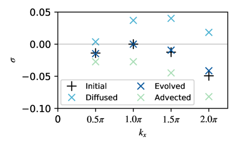
Figure 1: Eigenvalue spectra for $\mathrm{Ra}=10^{5}$. The spectrum of an “initial” marginally-stable mean temperature profile $\overline{T}(z,t_{0})$ has a maximum eigenvalue of 0. Given a small fixed timestep $\Delta t$, diffusion (equation 23) destabilizes the system, increasing $\sigma$. Advection (equation 24) tends to stabilize the system, decreasing $\sigma$. We find the eigenfunction amplitude $A^{2}$ such that the combination of diffusion and advection yields a new, “evolved,” marginally-stable mean temperature profile $\overline{T}(z,t_{0}+\Delta t)$. In this case $A^{2}\approx 1$ due to approximately equal magnitudes of the diffused and advected eigenvalues.

Consider a marginally-stable temperature profile $\overline{T}(z,t_{0})$. By definition, its maximum growth rate is 0. Diffusing $\overline{T}(z,t_{0})$ tends to increase its growth rates while ignoring the diffusive term and evolving according to advection tends to decrease its growth rates (see Figure 1). The amplitude $A$ must be selected such that these two influences are equal and opposite. We can measure the effects of diffusion and advection on the maximum growth rate by solving two new initial value problems

$$\frac{\partial\overline{T}_{\rm{diff}}}{\partial t}=\mathcal{P}\frac{\partial^{2}\overline{T}_{\rm{diff}}}{\partial z^{2}}$$ (23)

$$\frac{\partial\overline{T}_{\rm{adv}}}{\partial t}+2\frac{\partial}{\partial z}\Re\left[W\theta^{*}\right]=0$$ (24)

where $\overline{T}_{\rm{diff}}$ and $\overline{T}_{\rm{adv}}$ denote the diffused and advected temperature profiles respectively. In equation 24 we have set the amplitude of the eigenfunctions $A=1$ so we can determine how advection changes the temperature profiles. The factor of 2 arises due to the horizontal averaging of the advective term in (10).

We solve equations (23) & (24) from $t=t_{0}$ to $t=t_{0}+\Delta t$, initializing each temperature profile with $\overline{T}(z,t_{0})$. Suppose $k_{0}$ is the wavenumber of the marginally-stable mode. We then calculate the $k_{x}=k_{0}$ mode’s growth rates $\sigma_{\rm{diff}}$ and $\sigma_{\rm{adv}}$ for $\overline{T}_{\rm{diff}}$ and $\overline{T}_{\rm{adv}}$. A good guess for $A^{2}$ is

$$A^{2}\approx\Lambda^{2}_{0}\equiv-\frac{\sigma_{\rm{diff}}}{\sigma_{\rm{adv}}}.$$ (25)

This estimate follows from first-order perturbation theory. Note that $\sigma_{\rm{adv}}<0$ and $\sigma_{\rm{diff}}>0$, so $\Lambda_{0}^{2}>0$.

Using the approximate amplitude $\Lambda_{0}^{2}$, the background temperature $\overline{T}(z,t_{0})$ is then evolved to $t=t_{0}+\Delta t$ according to (10) and another eigenvalue solve is performed. This background temperature is typically close to, but not exactly, marginally-stable. In fact, in the limit $\Delta t\rightarrow 0$, the estimate $\Lambda_{0}^{2}$ approaches the amplitude $A^{2}$ necessary to keep the background temperature marginally-stable Michel and Chini (2019a). We use Newton’s method to find an amplitude $A^{2}$ such that the maximum growth rate is zero to within $10^{-9}$. Marginally-stable modes do not oscillate in time, i.e. $\sigma=0$ implies $\omega=0$. This agrees with the conventional notion of exchange of stabilities Drazin and Reid (2004). Crucially, we do not assume the $k_{x}$ of the marginally-stable mode is fixed. In Section III.1 we specify procedures for the treatment of multiple simultaneously marginal modes.

III.1 Treatment of Multiple Marginally-Stable Modes

In most cases, we encounter eigenvalue spectra with multiple marginal modes. To accommodate this we generalize the advective term in (10) to accommodate $N$ simultaneously marginal modes

$$\langle w^{\prime}T^{\prime}\rangle_{x}=\sum_{n=1}^{N}2A_{n}^{2}\Re\left[W_{n}\theta_{n}^{*}\right]$$ (26)

where $W_{n}$ and $\theta_{n}$ are the marginally-stable eigenmodes associated with different values of $k_{x}$. The factor of 2 is again due to horizontal averaging. There are now $N$ modes, each with their own amplitude to solve for and eigenvalue to keep marginally-stable. Given a small fixed time step $\Delta t$, let $\boldsymbol{A^{2}}$ be the amplitude vector and $\boldsymbol{\sigma}(\boldsymbol{A^{2}})$ be the eigenvalues of the $N$ modes. We are searching for $\boldsymbol{\tilde{A}^{2}}$ that satisfies $\boldsymbol{\sigma}(\boldsymbol{\tilde{A}^{2}})=0$. We approximate the amplitudes with $\boldsymbol{\Lambda^{2}_{0}}$ by generalizing (25):

$$\boldsymbol{\tilde{A}^{2}}\approx\boldsymbol{\Lambda^{2}_{0}}=-\Sigma_{\rm{adv}}^{-1}\boldsymbol{\sigma_{\rm{diff}}}.$$ (27)

Here $\boldsymbol{\sigma_{\rm{diff}}}=\boldsymbol{\sigma}(\boldsymbol{0})$ refers to the eigenvalues of the background temperature after evolving under only diffusion (equation 23) for a time interval $\Delta t$. We account for the influence of $N$ advection terms on $N$ eigenvalues (one for each mode) by constructing an eigenvalue matrix $\Sigma_{\rm{adv}}$. To calculate the element of $\Sigma_{\rm{adv}}$ at row $i$ and column $j$, we evolve the background temperature under only advection by mode $j$ for a time interval $\Delta t$. Then the $i,j$ component of $\Sigma_{\rm{adv}}$ is given by the eigenvalue of the $i$th mode.

Our estimate $\boldsymbol{\Lambda^{2}_{0}}$ does not typically give a background temperature for which all $N$ modes are exactly marginally-stable. We refine our vector of amplitudes via Newton’s method. This requires calculating the Jacobian matrix

$$J=\begin{bmatrix}\nabla\sigma_{1}(A_{1},A_{2},...,A_{N})\\ \nabla\sigma_{2}(A_{1},A_{2},...,A_{N})\\ \vdots\\ \nabla\sigma_{N}(A_{1},A_{2},...,A_{N})\end{bmatrix}.$$ (28)

We approximate $J$ via first-order finite differences, which requires an additional $N^{2}$ sparse eigenvalue solves. We iterate Newton’s method until all marginally-stable modes have eigenvalues within $10^{-9}$ of zero. We find $\boldsymbol{\sigma}(\boldsymbol{A^{2}})$ does indeed have a unique root provided the time step is not too large and there are no numerical instabilities, as outlined in Appendix B. Presumably this is due to the coupling of $\langle w^{\prime}T^{\prime}\rangle_{x}$ with $\overline{T}$. Over the course of a large time step, $\overline{T}$ evolves according to (10) and eventually the original eigenfunctions cease to provide a stabilizing influence. This limits the timestep size we can take.

Difficulty arises when transitioning between different numbers of marginal modes. We facilitate these transitions by defining an adjustable candidate tolerance $\varepsilon_{\rm{cand}}\in[10^{-6},10^{-8}]$. A mode which meets the candidate tolerance can be included in the subsequent timestep as a candidate marginal mode. Candidate modes are rejected when the root-finding algorithm converges on a negative amplitude $A^{2}<0$. Otherwise the mode becomes marginally-stable. In a similar manner, a marginally-stable mode need not remain marginally-stable. If its amplitude converges to some $A^{2}<0$ as before, then that mode is discarded and the timestep is repeated.

IV Properties of Thermally Equilibrated States

We evolve $\overline{T}$ as described above until $\max|\partial_{t}\overline{T}|<10^{-5}$. In this marginally-stable thermal equilibrium, $\overline{T}$ does not evolve in time, and the perturbations also do not evolve in time, as they are marginally-stable. Thus, these configurations are exact solutions to the quasilinear system (equations 10–14). They differ from the usual ECS in that ECS are fixed points of the full nonlinear problem (1)–(3). Such definitions are not mutually exclusive, but in general we can assume that MSTE and ECS are not steady with respect to their counterparts’ equations. We compute symmetric MSTE for $\mathrm{Ra}$ in the range $10^{5}-10^{9}$.

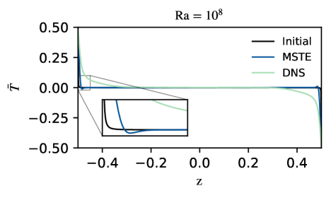
Figure 2: Mean temperature profiles $\overline{T}$ for $\mathrm{Ra}=10^{8}$. The initial profile is given by (35). We evolve this background temperature profile according to Section III until we reach a marginally-stable thermal equilibrium (MSTE). The DNS curve is obtained from a 2D nonlinear simulation of (1)–(3) with Dedalus. DNS temperature data are horizontally- and time-averaged. The initial profile has the narrowest boundary layer, while the DNS profile has the widest boundary layer. The MSTE profile exhibits prominent dips, nested alongside the boundary regions.

Figure 2 gives temperature profiles for $\mathrm{Ra}=10^{8}$, where the initial profile is outlined in Appendix A. We run a direct numerical simulation (DNS) of (1)–(3) with Dedalus and plot the horizontal- and time- averaged temperature profile. The temperature boundary layers in the DNS are wider than in the MSTE, which is in turn wider than the boundary layer of the initial temperature profile. Performing an eigenvalue solve by setting $\overline{T}$ equal to the DNS profile yields unstable eigenvalues. Every marginally-stable initial profile we experiment with ($\tanh$, $\rm{erf}$) has thinner boundary layers than the DNS and MSTE profiles. In conjunction, these two facts suggest that MSTE maximize boundary layer thickness while subject to the marginal stability constraint.

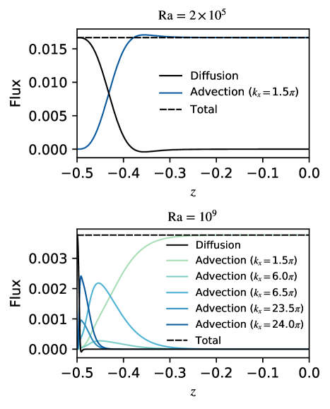
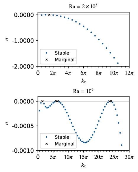
Figure 3: Heat fluxes (left) and eigenvalue spectra (right) of equilibrated states with $\mathrm{Ra}=2\times 10^{5}$ (top) and $\mathrm{Ra}=10^{9}$ (bottom). The heat flux profiles are symmetric about $z=0$, so we only plot for $z<0$. We plot the advection profiles for marginally-stable modes. At low $\mathrm{Ra}$, a single mode with $k_{x}=1.5\pi$ is sufficient to oppose boundary layer diffusion and facilitate heat flux throughout the bulk of the domain. At large $\mathrm{Ra}$, high-wavenumber modes contribute pronounced small-scale advection profiles which tightly hug the thin boundary layers. A combination of progressively wider advection profiles is necessary to transition to bulk advection provided by the $k_{x}=1.5\pi$ mode. This bulk mode mimics the large-scale convective cells which are characteristic of Rayleigh–Bénard convection, both in qualitative structure and number of cells in the domain. The eigenfunctions which compose the advective profiles are illustrated in Appendix D.

The most resilient and unexpected feature of MSTE temperature profiles are the pronounced dips adjacent to the boundary layers. These dips appear in every solution, regardless of $\mathrm{Ra}$. Physically, they correspond to thin layers in which the mean temperature gradient reverses, contradicting an important hypothesis of Malkus (1954). This counter-diffusion, which opposes overall heat transfer, is overcome by the coinciding advective flux, shown in Figure 3. We do not understand the source of these dips, but similar temperature gradient reversals were reported by Chini and Cox (2009) along the midlines of 2D convective cellular solutions at $\mathrm{Ra}\sim 10^{6}$. In that case, the reversals were due to nonlinear advection, which is not present in our quasilinear model.

In Figure 3, we give heat flux profiles and eigenvalue spectra for two cases: $\mathrm{Ra}=2\times 10^{5}$ (top) and $\mathrm{Ra}=10^{9}$ (bottom). Appendix D shows representative vertical velocity and temperature perturbation eigenfunctions. For $\mathrm{Ra}=2\times 10^{5}$, there is a single marginal mode at $k_{x}=1.5\pi$ whose advective flux occupies the bulk of the domain. These states have wide boundary layers, with diffusive fluxes which gradually subside as advection becomes the dominant flux component. Transitional regions occur over a smaller length scale for $\mathrm{Ra}=10^{9}$ where the shift from diffusion to advection is sharp. At $\mathrm{Ra}=10^{9}$ we find five marginally-stable modes are necessary to reach an MSTE. Thin advection profiles, belonging to high-wavenumber modes with $k_{x}=23.5\pi,\,24\pi$, hug the boundary layer. Closer to the bulk of the domain, we see wider advection profiles corresponding to modes in a second pair of marginal modes $k_{x}=6\pi,\,6.5\pi$. Adjacent pairs of marginal modes whose wavenumbers differ by $0.5\pi$ are common among MSTE. The isolated $k_{x}=1.5\pi$ mode forms the same arrangement and number of large-scale convective cells observed in DNS, again occupying the bulk of the domain. The pairs of modes $k_{x}=6\pi,\,6.5\pi$ and $k_{x}=23.5\pi,\,24\pi$ are each associated with a single maximum in our plots of growth rate $\sigma$ as a function of $k_{x}$ (lower right panel of Figure 3). If we allowed wavenumbers to vary continuously, there would be an unstable mode between these pairs of wavenumbers. However, since we have fixed the horizontal size of our domain, we are left with pairs of discrete marginal modes.

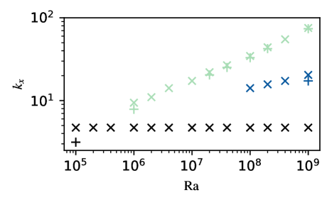
Figure 4: Wavenumbers of marginally-stable modes in thermally equilibrated states. Marginal modes often appear in adjacent pairs, which we denote with a common color. Within each of these pairs, the largest and smallest $k_{x}$ are denoted with an x and a + respectively. For example, the spectrum corresponding to $\mathrm{Ra}=10^{5}$ has adjacent marginal wavenumbers $k_{x}=\pi,\,1.5\pi$. The $\mathrm{Ra}=10^{9}$ spectrum, shown in the lower right corner of Figure 3, has three groups of maxima, with a single marginal mode in the first group ($k_{x}=1.5\pi$), two adjacent marginal modes in the second group ($k_{x}=6\pi,\,6.5\pi$), and two adjacent marginal modes in the third group ($k_{x}=23.5\pi,\,24\pi$). The largest wavenumbers of the green and blue branches depend on $\mathrm{Ra}$ according to power laws. For the green branch, $\max\{k_{x}\}\propto\mathrm{Ra}^{0.300}$ with $R^{2}=0.998$ while for the blue branch, $k_{x}\propto\mathrm{Ra}^{0.155}$ with $R^{2}=0.988$.

MSTE for large $\mathrm{Ra}$ tend to have a diverse combination of marginal modes. In every case, the $k_{x}=1.5\pi$ mode is included. In Figure 4 we give the wavenumbers $k_{x}$ of marginal modes. Adjacent pairs of marginal modes are common but not ubiquitous. Like $k_{x}=6\pi,\,6.5\pi$ and $k_{x}=23.5\pi,\,24\pi$ for the $\mathrm{Ra}=10^{9}$ MSTE, these are due to the discretization of wavenumbers from our domain of width 4. We think of the pairs of modes as acting together as part of a single maximum of the growth rate as a function of the wavenumber. When wavenumbers are adjacent, we plot them in the same color and denote the larger mode with an x and the smaller with a +. For $\mathrm{Ra}\geq 10^{6}$, a second branch of marginal modes is shown in light green. Least-squares regression gives $\max\{k_{x}\}\propto\mathrm{Ra}^{0.300}$ with $R^{2}=0.998$ for this maximum branch. For large $\mathrm{Ra}$, the advective fluxes of this maximum branch compensate for the strongly peaked diffusive flux in the thin boundary layers. At $\mathrm{Ra}\geq 10^{8}$, a third branch appears (shown in blue), splitting the widening gap between the other two. For these points regression gives $k_{x}\propto\mathrm{Ra}^{0.155}$ with $R^{2}=0.988$. The blue branch is associated with moderately wide advection profiles, filling a niche in the total flux by uniting the thin profiles of the maximum branch with those of the bulk-domain-oriented minimum branch.

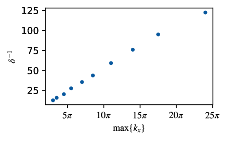
Figure 5: For $\mathrm{Ra}\geq 10^{6}$, the maximum marginally-stable wavenumber (corresponding to the green x markers in Figure 4) are inversely related to the boundary layer height $\delta$. $(\max\{k_{x}\})^{-1}$ gives a minimum $x$ length scale for the perturbations, and consequently, the advection. For large $\mathrm{Ra}$, the boundary layers admit small scale features, requiring more vertical basis functions (higher resolution, see Appendix C for specifications). The boundary layer height gives an estimate of the minimum vertical length scale in the problem. This suggests that the minimum horizontal and vertical length scales are proportional to each other over a wide range of $\mathrm{Ra}$.

The largest marginal wavenumber $\max\{k_{x}\}$ (represented by the light green branch in Figure 4) serves as an inverse minimum length scale in the $x$ direction. The finest vertical structures in $\overline{T}(z)$ appear near the boundaries, requiring more basis functions (resolution) at large $\mathrm{Ra}$. Naturally, this provides a complementary minimum length scale for $z$. We define the boundary layer height $\delta$ as the distance from the boundary where $\partial_{z}\overline{T}$ equals zero, i.e.,

$$\left.\frac{\partial\overline{T}}{\partial z}\right|_{z=-\frac{1}{2}+\delta}=0,\qquad 0<\delta<1/2.$$ (29)

This height corresponds to the local extrema of the MSTE temperature profile, e.g., in Figure 2. In Figure 5, we show $\max\{k_{x}\}$ is proportional to $\delta^{-1}$ over our range of $\mathrm{Ra}$. Least-squares regression gives $\delta^{-1}=1.71\max\{k_{x}\}-2.13$ with $R^{2}=0.996$.

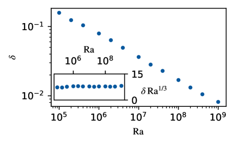
Figure 6: Boundary layer height $\delta$ of MSTE. We define the boundary layer height based off the location where $\frac{\partial\overline{T}}{\partial z}=0$ (see equation 29). Plotting on a log-log scale, we find that $\delta$ and $\mathrm{Ra}$ obey a power-law relationship. We also demonstrate that $\mathrm{Ra}^{1/3}\delta$ is approximately constant with respect to $\mathrm{Ra}$ which is consistent with Malkus (1954)

We find the MSTE can be characterized by their boundary layer height. In Figure 6, we illustrate the scaling behavior of the boundary layer height $\delta\sim\mathrm{Ra}^{-1/3}$. This is consistent with Malkus’ classical marginal stability theory, a scaling argument which perceives the boundary regions as subdomains which are themselves marginally-stable Malkus (1954).

The temperature boundary layers of MSTE exhibit self-similarity despite great variation in $\mathrm{Ra}$. We illustrate this in Figure 7 where the mean temperature $\overline{T}$ is plotted along a rescaled $z$-coordinate $\frac{z+1/2}{\delta}$. The rescaled boundary layer geometry appears intrinsic to the MSTE, possibly minimizing diffusion as previously hypothesized. This again highlights the importance of the boundary layer height’s dependence on $\mathrm{Ra}$.

Figure 7: Temperature boundary layer geometries of various MSTE. Rescaling according to the previously defined boundary layer height $\delta$ reveals self-similarity in the temperature boundary layers despite large variation in $\mathrm{Ra}$. The rescaled curves remain approximately self-similar for $z<0$.

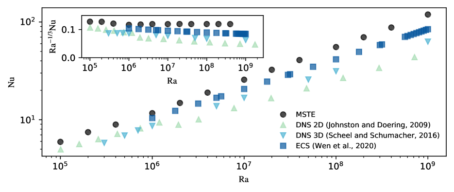
Figure 8: Nusselt numbers are shown for MSTE, aspect-ratio-optimized “steady rolls” ECS Wen et al. (2020), as well as statistically-steady 2D and 3D DNS Johnston and Doering (2009); Scheel and Schumacher (2016). All datasets obey power-law relationships, with the MSTE and ECS scaling like $\mathrm{Nu}\sim\mathrm{Ra}^{1/3}$. MSTE have greater $\mathrm{Nu}$ than the ECS, which in turn, have greater $\mathrm{Nu}$ than the DNS. This can be explained by the contrasting boundary layer geometries shown in Figure 2.

The Nusselt number, which measures convective performance is given by

$$\mathrm{Nu}=\frac{\langle\langle w^{\prime}T^{\prime}\rangle_{x}-\mathcal{P}\frac{\partial\overline{T}}{\partial z}\rangle_{z}}{\langle-\mathcal{P}\frac{\partial\overline{T}}{\partial z}\rangle_{z}}.$$ (30)

There is no general consensus surrounding the scaling behavior of $\mathrm{Nu}$ for high $\mathrm{Ra}$ systems, which are of particular importance in astrophysical and geophysical systems. In Figure 8 we report $\mathrm{Nu}$ for MSTE, “steady rolls” ECS Wen et al. (2020), and DNS Scheel and Schumacher (2016); Johnston and Doering (2009). We find that MSTE satisfy $\mathrm{Nu}\sim\mathrm{Ra}^{1/3}$, consistent with our finding that the boundary layer height scales like $\delta\sim\mathrm{Ra}^{1/3}$. The Nusselt numbers of the ECS are somewhat lower and the DNS Nusselt numbers are yet lower still. In both cases, the $\mathrm{Ra}$ dependence appear slightly more shallow than for the MSTE. Ref. Wen et al. (2020) hypothesized that the $\mathrm{Nu}$ of all ECS which admit classical Malkus scaling must always exceed the $\mathrm{Nu}$ of turbulent convection. If we generalize this notion to include quasilinear equilibria, our findings agree; MSTE have larger $\mathrm{Nu}$ than 2D and 3D DNS. This might be due to the chaotic transitions among the unstable periodic orbits outlined by Yalnız et al. (2020); Cvitanović and Gibson (2010) inhibiting heat flux. We might also anticipate the existence of similar equilibria with smaller $\mathrm{Nu}$, occupying complementary nodes in the Markov chain whose behavior agrees with DNS.

V Simulations with Thermally Equilibrated Initial Conditions

This investigation is partially motivated by the prospect of decreasing DNS runtimes by employing MSTE as initial conditions. One common choice of initial conditions for DNS of equations (1)–(3) are

$$T(x,z)\big{|}_{t=0} =0.5-z+\mathcal{N}$$

$$\boldsymbol{u}(x,z)\big{|}_{t=0} =\boldsymbol{0}$$

$$p(x,z)\big{|}_{t=0} =0$$ (31)

where $\mathcal{N}$ is low-amplitude random noise concentrated in the bulk of the domain. Here we instead initialize using the MSTE,

$$T(x,z)\big{|}_{t=0} =\overline{T}(z)+\sum_{n=1}^{N}A_{n}\Re\Big{[}\theta_{n}(z)e^{ik_{x_{n}}x}\Big{]}+\mathcal{N}$$

$$\boldsymbol{u}(x,z)\big{|}_{t=0} =\sum_{n=1}^{N}A_{n}\Re\Big{[}\Big{(}U_{n}(z)\hat{x}+W_{n}(z)\hat{z}\Big{)}e^{ik_{x_{n}}x}\Big{]}$$

$$p(x,z)\big{|}_{t=0} =\sum_{n=1}^{N}A_{n}\Re\Big{[}P_{n}(z)e^{ik_{x_{n}}x}\Big{]}$$ (32)

where $\theta_{n}(z),\,U_{n}(z),\,W_{n}(z),\,P_{n}(z);\;A_{n};$ and $k_{x_{n}}$ refer to the complex eigenfunctions, amplitude, and wavenumber of the $n$th marginal mode respectively. Note that although the MSTE is an equilibrium of the quasilinear equations, it is not an equilibrium of the full nonlinear equations. Accordingly the simulation state would evolve on initialization absent a random noise term. Here we include noise as a source of asymmetries. We also perform a simulation with MSTE absent any initial velocity ($\boldsymbol{u}(x,z)|_{t=0}=\boldsymbol{0}$). This state is not in equilibrium but we refer to it as “MSTE No Flow” for clarity.

Figure 9: Nusselt numbers of simulations performed at $\mathrm{Ra}=10^{8}$, initialized with the conductive equilibrium plus thermal noise (black), the MSTE (blue), and the MSTE absent initial flow (green). The MSTE simulation does not undergo a convective-transient period because the characteristic large-scale convective cell structure exists on initialization. The MSTE no flow simulation exhibits quasi-periodic oscillations in $\mathrm{Nu}$ which appear to persist for long times. The oscillations are great enough in amplitude that $\mathrm{Nu}$ is quasi-periodically negative, indicating brief periods of average heat transfer reversal.

Simulations initialized with the conductive equilibrium plus low-amplitude thermal noise have a large peak in $\mathrm{Nu}$ early on in their evolution (Figure 9). This is due to a burst of turbulence which occurs when the convective motions first become nonlinear. The MSTE no flow simulation undergoes a similar transient period, albeit less pronounced as illustrated by the smaller peak in the green curve. A simulation initialized with the MSTE, however, does not exhibit this transient burst of turbulence, as the large-scale anatomy of convective cells exists on initialization. Simulation of this transitional period is prohibitive Anders et al. (2018). For high $\mathrm{Ra}$ experiments, researchers often “bootstrap” data by initializing simulations with the results of similar $\mathrm{Ra}$ runs Verzicco and Camussi (1997); Johnston and Doering (2009). MSTE can be perceived as a set of initial conditions, designed for avoiding the simulation of transient high Reynolds number flows. MSTE absent velocity effectively achieve the same goal.

MSTE are laminar, lacking the small-scale structures associated with moderate- to high-$\mathrm{Ra}$ experiments. This is an apparent consequence of the quasilinear assumptions. If we perceive MSTE as background states, DNS suggest that plumes, vortex sheets, and other unstable turbulent features inhibit total heat transfer. This perspective agrees with conventional models of transitions to turbulent flows, such as Boussinesq’s turbulent-viscosity hypothesis Boussinesq (1877). The emergence of small-scale velocity structures is indicative of nonlinear energy transfer to small scales where energy is lost due to viscosity. Buoyancy driven flows are therefore impeded and the advection in the bulk of the domain decreases in magnitude Drazin and Reid (2004); Pope (2000). We could also attribute the diffuse DNS temperature profile in Figure 2 with unsteady boundary-layer penetration and mixing that MSTE do not exhibit.

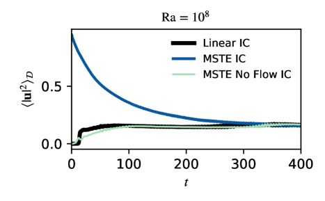
Figure 10: Average kinetic energies are reported for the same simulations illustrated in Figure 9 ($\mathrm{Ra}=10^{8}$). The eigenfunctions belonging to MSTE have significantly more kinetic energy than the statistically-steady state. Kinetic equilibrium is achieved on a long viscous time scale.

We also find that the average kinetic energy of the simulation initialized with MSTE is significantly larger than those found in either of the other cases, as shown Figure 10. This is because MSTE contain strong large-scale high-velocity flows, which decay on a long viscous time scale $t_{\nu}$. These powerful advective flows balance the heat flux in the bulk of the domain with the strong diffusion of thin MSTE temperature boundary layers. Fluid in the other cases is initialized at rest. Two viscous time scales can be derived for this problem: one for the boundary layer

$$t_{\nu,\delta} =\frac{\delta^{2}}{\mathcal{P}}=2.86$$ (33)

and another for the entire domain

$$t_{\nu,L} =\frac{L^{2}_{z}}{\mathcal{P}}=10^{4}.$$ (34)

Empirically, we find $t_{\nu}\approx 200$ suggesting the true kinetic energy decay time scale is based on a length scale $\ell\approx 0.14$ which is longer than the boundary layer height $\delta$ but shorter than the domain height $L_{z}$. Consequently, MSTE initial conditions do not reduce the simulation time required to achieve a statistically-steady state—rather they increase it considerably! This is alleviated by using no-flow MSTE initial conditions. The MSTE temperature state is a promising candidate initial condition for high-Rayleigh number convection simulations.

VI Discussion

In this paper we describe a new way to study Rayleigh–Bénard convection. We compute marginally-stable thermal equilibria (MSTE), which are equilibria of the quasilinear equations. To compute MSTE, we construct a marginally-stable mean temperature profile and evolve it according to the advective flux of its marginally-stable eigenfunctions, and its own diffusion. We assume that at least some modes are always in a marginally-stable configuration and all other modes are stable. The marginal stability constraint then fixes the ratio between advection and diffusion (eigenfunction amplitude $A^{2}$). We use standard root-finding algorithms to solve for the appropriate $A^{2}$ at each timestep until the combination of diffusive and advective flux sum to a constant. The MSTE calculation is a one-dimensional problem, combining eigenvalue solves, and the time evolution of the one-dimensional mean temperature profile. Thus, MSTE can be calculated on a single workstation.

The MSTE contain large-scale convective cell structures, and have $\mathrm{Nu}\sim\mathrm{Ra}^{1/3}$. These are similar to what has been found in experiments and direct numerical simulations. But MSTE also exhibit unique and unexpected features: mean temperature gradient-reversals/dips, high kinetic energy flows, and a larger $\mathrm{Nu}$ than other equilibrated solutions. When initializing with different mean temperature profiles, we find the same MSTE, suggesting these equilibria might be unique.

Simulations initialized with the MSTE (32) do not undergo an early convective transient period, but have faster flows when compared with DNS. From a dynamical systems perspective, unstable orbits depart from MSTE and approach the global attractor on a viscous time scale. This requires more computational effort to achieve relaxation when compared to the conventional conductive initial condition (31). Initializing with only the temperature state of the MSTE avoids an early convective transient, but does not have excessive large-scale flows. These states could be excellent initial conditions for high-Rayleigh number DNS.

Using the mean temperature in a statistically-steady DNS as a background state for an eigenvalue problem yields positive eigenvalues: the system is in a perpetual state of instability. Unstable modes tend to stabilize the system rapidly, creating a negative feedback loop whose average state is linearly unstable. Future work could adjust the marginal stability criterion to allow for moderately unstable modes. Should the fast and slow time scales not be entirely separate, these modes might persist for long times. This might lead to greater agreement with DNS.

Another significant difference with DNS is the treatment of shear in the boundary layers. At sufficiently high $\mathrm{Ra}$, the shear in the kinetic boundary layers could become unstable and turbulent Ahlers et al. (2009). This cannot occur in our quasilinear model because the background state has no velocity shear. One avenue for future work is to include a mean horizontal flow, which could develop boundary layer structures. In that case, we would search for states which also balance viscous and Reynolds stresses across the domain. Perturbations about this background state could include shear flow instabilities. Another approach would be to use the generalized quasilinear approximation, in which the background state includes both the mean and low-wavenumber temperature and velocity profiles Marston et al. (2016). This would allow for linear instabilities of the shear driven by low-wavenumber rolls, as we see in all MSTE. Generalized quasilinear calculations are inherently multi-dimensional, so they are more computationally expensive than the eigenvalue-based analysis used to find MSTE. Despite these limitations, our one-dimensional MSTE states capture many interesting features of convection.

Appendix A Initial Buoyancy Profile

We initialize the thermal-equilibration algorithm with an analytical thermal boundary layer equation, derived by Shishkina et al. (2015)

$$\overline{\mathcal{T}}_{0}(\xi) =\frac{\sqrt{3}}{4\pi}\log\frac{(1+a\xi)^{3}}{1+(a\xi)^{3}}+\frac{3}{2\pi}\arctan\Big{(}\frac{4\pi}{9}\xi-\frac{1}{\sqrt{3}}\Big{)}+\frac{1}{4}$$

$$\xi =\frac{z+1/2}{\delta_{0}}\geq 0,\qquad a=\frac{2\pi}{3\sqrt{3}}$$ (35)

where $\delta_{0}$ is a new measure of the boundary layer height ($\delta_{0}\neq\delta$ in general). This function is meant to describe the temperature near $z=-1/2$ so it does not pass through the origin. An appropriate initial mean temperature profile $\overline{T}_{0}$ must be odd-symmetric, i.e. $\overline{T}_{0}(z)=-\overline{T}_{0}(-z)$. Due to continuity, this implies $\overline{T}_{0}(0)=0$. Accordingly, we construct $\overline{T}_{0}(z)$ by translating $\overline{\mathcal{T}}_{0}(z)$ vertically to pass through the origin. We then take its odd-extension and include a scaling coefficient to satisfy the boundary conditions $\overline{T}_{0}(-1/2)=1/2$ and $\overline{T}_{0}(1/2)=-1/2$. The initial mean temperature profile is therefore given by

$$\overline{T}_{0}(z) =\frac{1}{2}\begin{cases}1-\frac{\overline{\mathcal{T}}_{0}\big{(}\frac{z+1/2}{\delta_{0}}\big{)}}{\overline{\mathcal{T}}_{0}\big{(}\frac{1}{2\delta_{0}}\big{)}}\quad-1/2\leq z\leq 0\\[14.22636pt] -1+\frac{\overline{\mathcal{T}}_{0}\big{(}\frac{1/2-z}{\delta_{0}}\big{)}}{\overline{\mathcal{T}}_{0}\big{(}\frac{1}{2\delta_{0}}\big{)}}\quad 0<z\leq 1/2.\end{cases}$$

We expect each $\mathrm{Ra}$ to be associated with a unique $\delta_{0}$ for which $\overline{T}_{0}(z)$ is marginally-stable. It should be noted that when experimenting with various initial profiles $(\tanh,\,\rm{erf})$, we obtain indistinguishable equilibrated states. Therefore these initial states lie in the MSTE basin of attraction with respect to the quasilinear system. This might also suggest that solutions are unique. An example of (35) is given by the blue curve in Figure 2.

Appendix B Timestep Management

To find MSTE, we advance $\overline{T}$ by timesteps of size $\Delta t$. For large $\Delta t$, we find the advective flux terms fail to provide a stabilizing influence. This is due to coupling between the eigenfunctions $W(z)$, $\theta(z)$ and the mean temperature profile $\overline{T}$. In the context of our algorithm, this effectively deletes the sought-after root of the maximum eigenvalue function $\sigma_{\rm{max}}(A^{2})$, causing the root-finding method to fail. This is not a numerical instability, rather, it is an inherent limitation of our timestepping algorithm. To curtail this, we halt the root-finding algorithms after 20 successive approximations, and reduce the timestep by a factor of 1.1, and try again.

The timestep must be also reduced to avoid a numerical instability. We find that for large $\Delta t$, after several hundred iterations, highly concave features develop in the advective flux term $\langle w^{\prime}T^{\prime}\rangle_{x}$ near $z=0$. Such features are undesired, as they are uncommon in similar calculations Malkus (1954) and we do not believe they accurately represent a physical process. If ignored, the concave features grow in magnitude until they affect $\overline{T}$ on a readily apparent scale. Eventually $\overline{T}$ develops oscillations near $z=0$ and the timestep must be reduced. Once these oscillations reach some amplitude, they cannot be eliminated via timestep reduction and the roots of $\sigma_{\rm{max}}(A^{2})$ vanish. To avoid this, we measure the curvature of the advective flux $|\frac{\partial^{2}}{\partial z^{2}}\langle w^{\prime}T^{\prime}\rangle_{x}|_{z=0}|$ of the dominant $k_{x}=1.5\pi$ mode. We find that reducing the timestep $\Delta t$ by the same factor of 1.1 whenever this curvature measure exceeds $10^{-6}$ curtails the problem. Both of these issues appear to become more prominent as the boundary layers diffuse over the course of the algorithm’s execution (see Figure 2). Thus there is never a practical opportunity to increase the timestep.

Appendix C MSTE Parameters and Results

Table 1: Control parameters and results are given for the MSTE timestepping algorithm. $N_{z}$ denotes the number of Chebyshev basis functions employed. This, along with $\mathrm{Ra}$ are specified on initialization. The remaining quantities are computed directly from the MSTE. The low $\mathrm{Ra}=10^{5}$ case requires $\sim 12$ hours to compute while the high $\mathrm{Ra}=10^{9}$ case requires $\sim 72$ hours. Eigenvalue solves are performed for various $k_{x}$ simultaneously using 28 cores.

$\mathrm{Ra}$	$N_{z}$	$\mathrm{Nu}$	$\delta$	marginal $k_{x}$
$10^{5}$	256	5.9343	0.15746	1$\pi$, 1.5$\pi$
$2\times 10^{5}$	256	7.45986	0.12341	1.5$\pi$
$4\times 10^{5}$	256	8.92597	0.10395	1.5$\pi$
$10^{6}$	256	11.6689	0.07922	1.5$\pi$, 2.5$\pi$, 3$\pi$
$2\times 10^{6}$	256	14.8463	0.06345	1.5$\pi$, 3.5$\pi$
$4\times 10^{6}$	256	18.9433	0.04933	1.5$\pi$, 4.5$\pi$
$10^{7}$	256	25.6821	0.03632	1.5$\pi$, 5.5$\pi$
$2\times 10^{7}$	256	32.4531	0.02820	1.5$\pi$, 6.5$\pi$, 7$\pi$
$4\times 10^{7}$	512	40.7925	0.02289	1.5$\pi$, 8$\pi$, 8.5$\pi$
$10^{8}$	512	55.4383	0.01690	1.5$\pi$, 4.5$\pi$, 10.5$\pi$, 11$\pi$
$2\times 10^{8}$	512	69.8349	0.01318	1.5$\pi$, 5$\pi$, 13.5$\pi$, 14$\pi$
$4\times 10^{8}$	512	87.8525	0.01053	1.5$\pi$, 5.5$\pi$,17.5$\pi$
$10^{9}$	768	119.318	0.00817	1.5$\pi$, 6.0$\pi$, 6.5$\pi$, 23.5$\pi$, 24$\pi$

Appendix D MSTE Eigenfunctions

In Figure 11 we plot the velocity and temperature perturbation eigenfunctions for the marginally-stable modes in the $\mathrm{Ra}=10^{9}$ MSTE. Though the eigenfunctions are in general complex, the linear system (12)–(14) obeys phase-shift symmetry. Any set of solutions can be phase-shifted by multiplying the perturbations by a complex quantity of unit modulus $e^{i\phi}$. In this particular case, we can eliminate the perturbations’ imaginary components by selecting the proper $\phi$. This is due to the exchange of stabilities mentioned previously: $\omega=0$ at marginal stability implies that the system admits a set of real solutions. Adjacent modes, whose wavenumbers only differ by $0.5\pi$, are superimposed to illustrate their similarity. For the large-scale $k_{x}=1.5\pi$ mode, we find the vertical velocity eigenfunction $W$ is maximized near the center of the domain. As $k_{x}$ increases, we observe two vertical velocity maxima, each tending towards their respective boundary. However, in all cases, the temperature perturbations are more concentrated at the boundaries than the vertical velocity. This trend is also apparent in the two pairs of adjacent modes. In the temperature eigenfunctions $\theta$, small-scale zig-zags appear near the boundaries at $k_{x}=1.5\pi$, subsiding as $k_{x}$ increases. The left-most peaks of these temperature perturbation profiles approximately coincide with the previously-defined boundary layer height $\delta$.

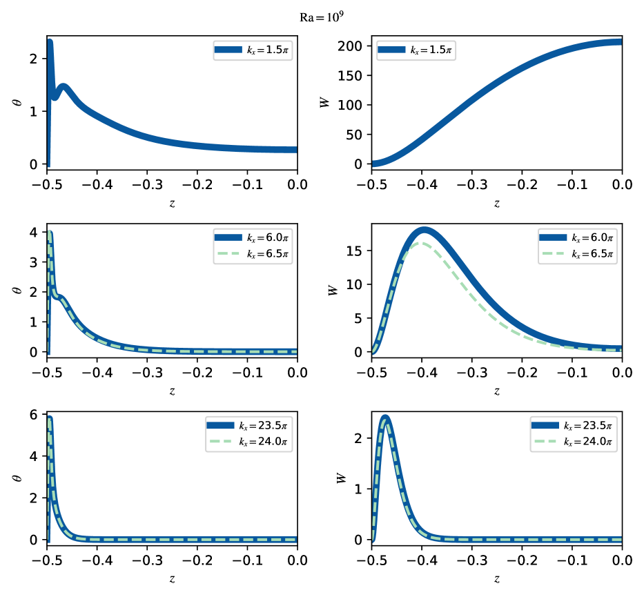
Figure 11: The temperature and pressure MSTE eigenfunctions are shown in separate plots for various marginally-stable modes. The eigenfunctions are normalized such that $\langle|\theta|^{2}\rangle_{\mathcal{D}}=1$. We select a phase such that the eigenfunctions are real. In this case the eigenfunctions are even which we exploit by plotting over half the domain.

References

- Couston et al. (2020) L.-A. Couston, D. Lecoanet, B. Favier, and M. Le Bars, Phys. Rev. Research 2, 023143 (2020).
- Zhu et al. (2018) X. Zhu, V. Mathai, R. J. Stevens, R. Verzicco, and D. Lohse, Physical Review Letters 120 (2018), 10.1103/physrevlett.120.144502.
- Ossendrijver (2003) M. Ossendrijver, Astronomy & Astrophysics Reviews 11, 287 (2003).
- Gubbins (2001) D. Gubbins, Physics of the Earth and Planetary Interiors 128, 3 (2001), dynamics and Magnetic Fields of the Earth’s and Planetary Interiors.
- Malkus (1954) W. V. R. Malkus, Proceedings of the Royal Society of London. Series A, Mathematical and Physical Sciences 225, 196 (1954).
- Howard (1966) L. N. Howard, in Applied Mechanics, edited by H. Görtler (Springer Berlin Heidelberg, Berlin, Heidelberg, 1966) pp. 1109–1115.
- Kraichnan (1962) R. H. Kraichnan, Physics of Fluids 5, 1374 (1962).
- Spiegel (1962) E. A. Spiegel, Journal of Geophysical Research 67, 3063 (1962).
- Castaing et al. (1989) B. Castaing, G. Gunaratne, L. Kadanoff, A. Libchaber, and F. Heslot, Journal of Fluid Mechanics 204, 1 (1989).
- Grossmann and Lohse (2000) S. Grossmann and D. Lohse, Journal of Fluid Mechanics 407, 27–56 (2000).
- Ahlers et al. (2009) G. Ahlers, S. Grossmann, and D. Lohse, Rev. Mod. Phys. 81, 503 (2009).
- Julien and Knobloch (2007) K. Julien and E. Knobloch, Journal of Mathematical Physics 48, 065405 (2007).
- Julien et al. (2012) K. Julien, E. Knobloch, A. M. Rubio, and G. M. Vasil, Phys. Rev. Lett. 109, 254503 (2012).
- Waleffe et al. (2015) F. Waleffe, A. Boonkasame, and L. Smith, Physics of Fluids 27, 051702 (2015).
- Sondak et al. (2015) D. Sondak, L. M. Smith, and F. Waleffe, Journal of Fluid Mechanics 784, 565 (2015), arXiv:1507.03151 [physics.flu-dyn] .
- Wen et al. (2020) B. Wen, D. Goluskin, and C. Doering, (2020).
- Chini and Cox (2009) G. P. Chini and S. Cox, Physics of Fluids 21, 083603 (2009).
- Yalnız et al. (2020) G. Yalnız, B. Hof, and N. Burak Budanur, arXiv e-prints , arXiv:2007.02584 (2020), arXiv:2007.02584 [physics.flu-dyn] .
- Cvitanović and Gibson (2010) P. Cvitanović and J. Gibson, Physica Scripta 2010, 014007 (2010).
- Marston et al. (2016) J. B. Marston, G. P. Chini, and S. M. Tobias, Phys. Rev. Lett. 116, 214501 (2016), arXiv:1601.06720 [physics.flu-dyn] .
- Beaume et al. (2015) C. Beaume, G. P. Chini, K. Julien, and E. Knobloch, Physical Review E 91 (2015), 10.1103/physreve.91.043010.
- Michel and Chini (2019a) G. Michel and G. P. Chini, Proceedings of the Royal Society A: Mathematical, Physical and Engineering Sciences 475, 20180630 (2019a).
- F.R.S. (1916) L. R. O. F.R.S., The London, Edinburgh, and Dublin Philosophical Magazine and Journal of Science 32, 529 (1916).
- Michel and Chini (2019b) G. Michel and G. P. Chini, Journal of Fluid Mechanics 858, 536–564 (2019b).
- Burns et al. (2020) K. J. Burns, G. M. Vasil, J. S. Oishi, D. Lecoanet, and B. P. Brown, Physical Review Research 2, 023068 (2020), arXiv:1905.10388 [astro-ph.IM] .
- Oishi et al. (2021) J. Oishi, K. Burns, S. Clark, E. Anders, B. Brown, G. Vasil, and D. Lecoanet, “Eigentools: Tools for studying linear eigenvalue problems,” (2021), ascl:2101.017 .
- Drazin and Reid (2004) P. G. Drazin and W. H. Reid, Hydrodynamic Stability, 2nd ed., Cambridge Mathematical Library (Cambridge University Press, 2004).
- Johnston and Doering (2009) H. Johnston and C. R. Doering, Phys. Rev. Lett. 102, 064501 (2009).
- Scheel and Schumacher (2016) J. D. Scheel and J. Schumacher, Journal of Fluid Mechanics 802, 147–173 (2016).
- Anders et al. (2018) E. H. Anders, B. P. Brown, and J. S. Oishi, Phys. Rev. Fluids 3, 083502 (2018).
- Verzicco and Camussi (1997) R. Verzicco and R. Camussi, Physics of Fluids 9, 1287 (1997), https://doi.org/10.1063/1.869244 .
- Boussinesq (1877) J. Boussinesq, (1877).
- Pope (2000) S. B. Pope, Turbulent Flows (Cambridge University Press, 2000).
- Shishkina et al. (2015) O. Shishkina, S. Horn, S. Wagner, and E. S. C. Ching, Phys. Rev. Lett. 114, 114302 (2015).