Mass scaling of the near-critical 2D Ising model using random currents

Abstract

We examine the Ising model at its critical temperature with an external magnetic field $ha^{\frac{15}{8}}$ on $a\mathbb{Z}^{2}$ for $a,h>0$. A new proof of exponential decay of the truncated two-point correlation functions is presented. It is proven that the mass (inverse correlation length) is of the order of $h^{\frac{8}{15}}$ in the limit $h\to 0$. This was previously proven with CLE-methods in [1]. Our new proof uses instead the random current representation of the Ising model and its backbone exploration. The method further relies on recent couplings to the random cluster model [2] as well as a near-critical RSW-result for the random cluster model [3].

1 Introduction

The square lattice Ising model [4] suggested by Lenz [5] is the archetypal statistical physics model undergoing an order/disorder phase transition. It has been subject of intense study in the past century [6, 7], starting with Periels’ proof of the existence of a phase transition [8] and Onsager’s calculation of the free energy [9]. The rigorous understanding of the critical two-dimensional Ising model has advanced tremendously in the past decade starting with the breakthroughs [10, 11] and with the subsequent works (see, for example, [12]).

One of the questions that remained unsolved until recently is obtaining the speed of the decay of the truncated correlations in the near-critical two-dimensional Ising model. For $a\in(0,1]$ and $h>0$ the near critical regime is defined to be the Ising measure on the lattice $a\mathbb{Z}^{2}$ with the parameter $\beta=\beta_{c}(\mathbb{Z}^{2})$ and external field $a^{15/8}\,h$. We denote the corresponding correlation functions with $\langle.\rangle_{a,h}$. The following theorem is proved in [1] using the scaling limit of the FK-Ising model which was proved to exist in [13] and its connections to the conformal loop ensemble [14]. See also the review [15].

Theorem 1.1.

There exists $B_{0},C_{0}\in(0,\infty)$ such that for any $a\in(0,1]$ and $h>0$ with $ha^{\frac{15}{8}}\leq 1$,

$$0\leq\langle\sigma_{x}\sigma_{y}\rangle_{a,h}-\langle\sigma_{x}\rangle_{a,h}\langle\sigma_{y}\rangle_{a,h}\leq C_{0}a^{\frac{1}{4}}\left|x-y\right|^{-\frac{1}{4}}e^{-B_{0}h^{\frac{8}{15}}\left|x-y\right|}.$$

Accordingly, for $a=1$ the result on $\mathbb{Z}^{2}$ is that for any $h\in [0,1)$,

$$\langle\sigma_{y}\sigma_{x}\rangle_{1,h}-\langle\sigma_{y}\rangle_{1,h}\langle\sigma_{x}\rangle_{1,h}\leq C_{0}\left|x-y\right|^{-\frac{1}{4}}e^{-B_{0}h^{\frac{8}{15}}\left|x-y\right|}.$$

In this paper we prove Theorem 1.2 from which we can deduce Theorem 1.1.

Theorem 1.2.

For any $h>0$ and $a\leq 1$ there are functions $C(h)>0$ and $m(h)>0$ independent of $a>0$ such that for any $x,y\in a\mathbb{Z}^{2}$ it holds that

$$\langle\sigma_{x}\sigma_{y}\rangle_{a,h}-\langle\sigma_{x}\rangle_{a,h}\langle\sigma_{y}\rangle_{a,h}\leq C(h)a^{\frac{1}{4}}\left|x-y\right|^{-\frac{1}{4}}e^{-m(h)\left|x-y\right|}.$$

The proof uses first a partial exploration of the backbone of random currents, then a recent coupling between the random current measure with sources and the random cluster model [2]. The proof utilises a new result that extends a result on crossing probabilities for the critical random cluster model to the near critical regime [3].

Before diving into the details, we briefly show how Theorem 1.1 follows (as explained in [1]) from Theorem 1.2.

Proof of Theorem 1.1.

Let $H$ be such that $a=H^{\frac{8}{15}}$ and $h=1$. Let $\langle\sigma_{0};\sigma_{x}\rangle=\langle\sigma_{0}\sigma_{x}\rangle_{a,h}-\langle\sigma_{0}\rangle_{a,h}\langle\sigma_{x}\rangle_{a,h}$. Then from Theorem 1.2

$$\langle\sigma_{0};\sigma_{x}\rangle_{H^{\frac{8}{15}},1}\leq C(1)H^{\frac{2}{15}}\left|x\right|^{-\frac{1}{4}}e^{-m(1)\left|x\right|}$$

for $x\in H^{\frac{8}{15}}\mathbb{Z}^{2}$. Using the relation $\langle\sigma_{0};\sigma_{x}\rangle_{H^{\frac{8}{15}},1}=\langle\sigma_{0};\sigma_{x^{\prime}}\rangle_{1,H}$ whenever $x^{\prime}=\frac{x}{H^{\frac{8}{15}}}$ we obtain

$$\langle\sigma_{0};\sigma_{x^{\prime}}\rangle_{1,H}\leq C(1)\left|x^{\prime}\right|^{-\frac{1}{4}}e^{-mH^{\frac{8}{15}}\left|x^{\prime}\right|}$$

for $x^{\prime}\in\mathbb{Z}^{2}$. Rescaling back to $a\mathbb{Z}^{2}$ yields the result. ∎

In [1] a converse inequality is also proved using reflection positivity. A more probabilistic proof of the lower bound was given in [16]. We note that this shows that the correlation length is finite, the mass gap exists and that critical exponent of the correlation length equals $\frac{8}{15}$. Further, as it is explained in [1] the exponential decay proven in Theorem 1.1 directly translates into the scaling limit.

Indeed, as in [1] if $\Phi^{a,h}$ is the near critical magnetization field given by

$$\Phi^{a,h}=a^{ \frac{15}{8}}\sum_{x\in a\mathbb{Z}^{2}} \sigma_{x}\delta_{x}$$

with $\{\sigma_{x}\}_{x\in a\mathbb{Z}^{2}}\in\{0,1\}^{a\mathbb{Z}^{2}}$, it was proven in Theorem 1.4 of [13]  that $\Phi^{a,h}$ converges in law to a continuum (generalized) random field $\Phi^{h}$. Let $C_{0}^{\infty}(\mathbb{R}^{2})$ denote the set of smooth functions with compact support and let $\Phi^{h}(f)$ be $\Phi^{h}$ paired against $f\in C_{0}^{\infty}(\mathbb{R}^{2})$. Then as in  [1] it holds that

Corollary 1.3.

Let $f,g\in C_{0}^{\infty}(\mathbb{R}^{2})$, then there are $B_{0},C_{0}\in(0,\infty)$ such that

$$\left|\text{Cov}(\Phi^{h}(f),\Phi^{h}(g))\right|\leq C_{0}\int\int_{\mathbb{R}^{2}\times\mathbb{R}^{2}} \left|f(x)\right|\left|g(x)\right|\left|x-y\right|^{- \frac{1}{4}} e^{-B_{0}h^{\frac{8}{15}}\left|x-y\right|}dxdy.$$

Starting with [17], there has in the physics community been much interest in the masses of the Ising model [18] including possible connections to the exceptional Lie Algebra $E_{8}$ [19] which has been investigated also experimentally [20, 21, 22] and numerically [23]. On the mathematical side, exponential decay was first rigorously proven in [24] and in [25] a linear upper bound for the mass was proven. Proving the correct scaling exponent is a further step towards rigorous results in this direction. For further rigorous developments see also [26].

2 Preliminaries

We start by briefly introducing the Ising model and its random cluster and random current representations that we will use to prove the result. Let $G=(V,E)$ be a finite graph. Then for each spin configuration $\sigma\in\{\pm 1\}^{V}$ and $h\geq 0$ define the energy

$$H(\sigma)=-\sum_{xy\in E}\sigma_{x}\sigma_{y}-h\sum_{x\in V}\sigma_{x},$$

where $h$ describes the effect of an external magnetic field. For each $A\subset V$ we let $\sigma_{A}=\prod_{x\in A}\sigma_{x}$ and define the correlation function as

$$\langle\sigma_{A}\rangle=\frac{\sum_{\sigma\in\{\pm 1\}^{V}}\sigma_{A}\exp(-\beta H(\sigma))}{Z}$$

where $Z=\sum_{\sigma\in\{\pm 1\}^{V}}\exp(-\beta H(\sigma))$ is the partition function. In what follows, we will be concerned with the Ising model on the graph $a\mathbb{Z}^{2}$ which is obtained by taking the thermodynamics limit of finite graphs. For discussions about the thermodynamic limit we refer the reader to [27].

In both representations we implement the magnetic field using Griffiths’ ghost vertex $\mathrm{g}$. This means that we consider the graph $G_{\text{ghost}}=(V\cup\{\mathrm{g}\},E\cup E_{\mathrm{g}})$ where $E_{\mathrm{g}}=\cup_{v\in V} \{e_{v\mathrm{g}}\}$ are additional edges from every original vertex $v$ to the ghost vertex $\mathrm{g}$ (see for example [7]). We will refer to the edges $E$ as internal edges and to the edges $E_{\mathrm{g}}$ as ghost edges.

The random current representation

Let us now introduce the random current representation which is a very effective tool in the study of the Ising model [28, 29, 30, 2, 31, 32, 33, 34]. Further information can be found in [7] and [35]. The central building blocks in the random current representation of the Ising model on a graph $G_{\text{ghost}}=(V\cup\{\mathrm{g}\},E\cup E_{\mathrm{g}})$ are the currents $\mathbf{n}\in{\mathbb{N}_{0}}^{E\cup E_{\mathrm{g}}}$. For each current $\mathbf{n}$ we can define its sources $\partial\mathbf{n}$ as the $v\in V$ where $\sum_{xv\in E\cup E_{g}}\mathbf{n}_{xv}$ is odd. Let further the weight of each current $\mathbf{n}$ be given by

$$w(\mathbf{n})=\prod_{xy\in E}\frac{\beta^{\mathbf{n}_{xy}}}{\mathbf{n}_{xy}!}\prod_{x\mathrm{g}\in E_{\mathrm{g}}}\frac{(\beta h)^{\mathbf{n}_{x\mathrm{g}}}}{\mathbf{n}_{x\mathrm{g}}!}.$$

A simple identity which connects the random currents to the Ising model is given as (2.4a) in [31]

$$\langle\sigma_{0}\sigma_{x}\rangle=\frac{\sum_{\partial\mathbf{n}=\{0,x\}}w(\mathbf{n})}{\sum_{\partial\mathbf{n}=\emptyset}w(\mathbf{n})}.$$ (1)

Further, given a current $\mathbf{n}$ define the traced current $\hat{\mathbf{n}}\in\{0,1\}^{E\cup E_{\mathrm{g}}}$ by $\hat{\mathbf{n}}(e)=0$ if $\mathbf{n}(e)=0$ and $\hat{\mathbf{n}}(e)=1$ if $\mathbf{n}(e)>0$. Then $\mathbb{P}_{G}^{A}$, the random current measure with sources $A\subset V$, is the probability measure that satisfies $\mathbb{P}_{G}^{A}(\mathbf{n})\propto w(\mathbf{n})1_{\{\partial\mathbf{n}=A\}}.$ If $A$ and $B$ are either vertices in or subsets of $V\cup\{g\}$ we denote the event that they are connected in a configuration $\omega\in\{0,1\}^{E \cup E_{\mathrm{g}}}$ by $A\leftrightarrow B$, meaning that one vertex of $A$ is connected to one vertex of $B$.

The traced random current measure $\hat{\mathbb{P}}_{G}^{A}$ gives each $\omega\in\{0,1\}^{E \cup E_{g}}$ the probability

$$\hat{\mathbb{P}}_{G}^{A}(\omega)=\sum_{\partial\mathbf{n}=A} \mathbb{P}_{G}^{A}(\mathbf{n})1_{\{\hat{\mathbf{n}}=\omega\}}.$$

To ease the notation in what follows define $\hat{\mathbb{P}}_{G}^{\{0,x\}}\otimes\hat{\mathbb{P}}_{G}^{\emptyset}$ to be the probability measure which assigns each $\omega\in\{0,1\}^{E\cup E_{\mathrm{g}}}$ the probability

$$\hat{\mathbb{P}}_{G}^{\{0,x\}}\otimes\hat{\mathbb{P}}_{G}^{\emptyset}(\omega)=\frac{1}{Z_{\emptyset}Z_{\{0,x\}}}\sum_{\partial\mathbf{n}=\{0,x\},\partial\mathbf{m}=\emptyset}w(\mathbf{n})w(\mathbf{m})1[\widehat{\mathbf{n}+\mathbf{m}}=\omega].$$

On the square lattice $a\mathbb{Z}^{2}$ in a magnetic field $a^{15/8}\,h$ we denote the non traced and traced single current measures by $\mathbb{P}_{a,h}^{A}$ and $\hat{\mathbb{P}}_{a,h}^{A}$ respectively. The main part of what follows proves exponential decay of truncated correlations, but first we obtain the correct front factor $a^{\frac{1}{4}}$. We do a similar trick as in [1] where we set the magnetic field $h$ to $0$ in the boxes of radius 1 around $0$ and $x$ and call that magnetic field $\vec{h}$.

Proposition 2.1.

We have

$$\langle\sigma_{0};\sigma_{x}\rangle_{a,h}\leq\langle\sigma_{0};\sigma_{x}\rangle_{a,\vec{h}}=\langle\sigma_{0}\sigma_{x}\rangle_{a,\vec{h}}\cdot\hat{\mathbb{P}}^{\{0,x\}}_{a,\vec{h}}\otimes\hat{\mathbb{P}}^{\emptyset}_{a,\vec{h}}(0\not\leftrightarrow\mathrm{g})\leq Ca^{\frac{1}{4}}\hat{\mathbb{P}}^{\{0,x\}}_{a,\vec{h}}(0\not\leftrightarrow\mathrm{g}).$$

Proof.

The first inequality follows from the GHS inequality [36]. The second step used the switching lemma [36] and (1). Since the event $\{0\not\leftrightarrow\mathrm{g}\}$ is decreasing the probability increases when $\hat{\mathbb{P}}^{\emptyset}_{a,\vec{h}}$ is removed. Then the last inequality is a standard application of equation (1-arm) below (see also [37]). ∎

The random cluster model

Each configuration $\omega\in\{0,1\}^{E\cup E_{\mathrm{g}}}$ corresponds to a (spanning) subgraph of $G_{ghost}$. For each $e\in E \cup E_{\mathrm{g}}$ if $w_{e}=1$ we say that $e$ is open and if $w_{e}=0$ we say that $e$ is closed. There is a natural partial order $\preceq$ on the configurations where $\omega\preceq\omega^{\prime}$ if $\omega^{\prime}$ can be obtained from $\omega$ by opening edges. An event $\mathcal{A}$ is increasing if for any $\omega\in\mathcal{A}$ it holds that $\omega\preceq\omega^{\prime}$ implies $\omega^{\prime}\in\mathcal{A}$. Let further $k(\omega)$ be the number of clusters of vertices of the configuration $\omega$.

The random cluster model with free boundary conditions $\phi_{G}^{0}$ is a percolation measure on the finite graph $G_{ghost}=(V\cup\{\mathrm{g}\},E\cup E_{\mathrm{g}})$ such that for every $\omega\in\{0,1\}^{E\cup E_{\mathrm{g}}}$

$$\phi_{G}^{0}({\omega})\propto 2^{k(\omega)}\prod_{e\in E \cup E_{\mathrm{g}}}\frac{p_{e}}{1-p_{e}}$$

where $p_{e}=1_{\{e\text{ is internal and open}\} }(1-\exp(-2\beta))+1_{\{e\text{ is ghost edge and open}\}}(1-\exp(-2\beta h))+\frac{1}{2} 1_{\{e\text{ closed}\}}$. In what follows, we will consider the free random cluster model on some finite subsets $\Lambda$ of $a\mathbb{Z}^{2}$ and we will denote that measure by $\phi_{\Lambda}^{a}$ at the same time fixing $\beta=\beta_{c}=\frac{\log(1+\sqrt{2})}{2}$ . Let $\Lambda_{k}(x)$ denote the box of with side length $k$ around some point $x\in a\mathbb{Z}^{2}$ and let $\Lambda_{k}=\Lambda_{k}(0)$. Notice that $\Lambda_{k}$ only depends on the distance in $\mathbb{R}^{2}$ which is not affected when $a$ changes. Further, let $A_{n,m}(x)=\Lambda_{m}(x)/\Lambda_{n}(x)$ be the $(n,m)$ annulus around $x$ and $A_{n,m}=A_{n,m}(0)$. The random cluster model has many nice properties that we will use in what follows. Since the boundary conditions are free the random cluster model has stochastic domination in terms of the domain. This means that if $\Lambda_{1}\subset\Lambda_{2}$ then for any increasing event $\mathcal{A}$,

$$\phi_{\Lambda_{1}}^{a}(\mathcal{A})\leq\phi_{\Lambda_{2}}^{a}(\mathcal{A}).$$ (MON)

Further, the (FKG)-inequality [7, Theorem 1.6] states that for increasing events $\mathcal{A},\mathcal{B}$ then

$$\phi_{\Lambda}^{a}(\mathcal{A}\cap\mathcal{B})\geq\phi_{\Lambda}^{a}(\mathcal{A})\phi_{\Lambda}^{a}(\mathcal{B}).$$ (FKG)

We note that the 1-arm exponent for the random cluster model [37, Lemma 5.4] is given by

$$C_{1}a^{\frac{1}{8}}\leq\phi_{\Lambda_{1}}^{a}(0\leftrightarrow\partial\Lambda_{1})\leq C_{2}a^{\frac{1}{8}}.$$ (1-arm)

The following result was proven in [1] and it will also prove useful for us.

Lemma 2.2.

([1], Proposition 1) Suppose that configuration of internal edges $\omega$ has clusters $C_{1},\dots,C_{n}$. Then

$$\phi^{a}_{\Lambda_{3}}(C_{i}\leftrightarrow\mathrm{g}|\omega)=\tanh(ha^{\frac{15}{8}}\left|C_{i}\right|)$$

and the events $\{C_{i}\leftrightarrow\mathrm{g}\}$ given $\omega$ are mutually independent.

Finally, we state a connection between the random currents with sources and the random cluster model.

Theorem 2.3.

([2], Theorem 3.2) Let $\{X(e)\}_{e\in E}$ be independent Bernoulli percolation with parameter $(1-\exp(-\beta_{e}))$ with $\beta_{e}=\beta$ for $e\in E$ and $\beta_{e}=\beta h$ for $e\in E_{\mathrm{g}}$. Then define for each $e\in E\cup E_{\mathrm{g}}$ the configuration

$$\omega(e)=\max\{\hat{\mathbf{n}}(e),X(e)\}.$$

where $\hat{\mathbf{n}}$ has the law of ${\hat{\mathbb{P}}}^{\{x,y\}}$ the traced random current with sources $\partial\mathbf{n}=\{x,y\}$. Then $\omega$ has the law of $\phi_{G}^{0}(\cdot\mid x\leftrightarrow y)$ which is the random cluster measure conditioned on $\{x\leftrightarrow y\}$. Hence, if $\mathcal{A}$ is a decreasing event then

$${\hat{\mathbb{P}}}^{\{x,y\}}(\mathcal{A})\geq\phi_{G}^{0}(\mathcal{A}\mid x\leftrightarrow y).$$

A key part in our result is the backbone exploration which we turn to next.

[capbesideposition=left,top,capbesidewidth=4cm]figure[]  

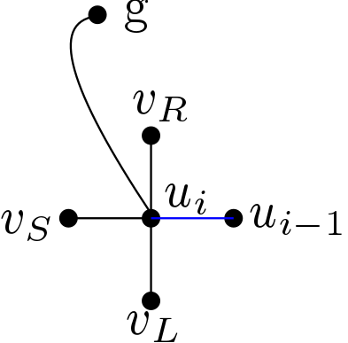
Figure 1: The situation in the backbone exploration with the incoming edge $e_{u_{i-1},u_{i}}$ coloured blue. The vertices $v_{R},v_{L},v_{S}$ are respectively to the right, left and straight of $u_{i}$ with respect to the incoming edge. As usual $\mathrm{g}$ denotes the ghost.

Backbone exploration

Let us first define the partially explored backbone. Suppose that $\mathbf{n}$ is some current with sources $\partial\mathbf{n}=\{x,y\}$. Then there is a path between $x$ and $y$ with $\mathbf{n}(e)$ odd for all edges $e$ along the path. The backbone is an algorithmic way of step-by-step constructing such a path until it hits some set of vertices $A\supset\{\mathrm{g},y\}$ . To do that, we define the sets of (explored) edges $\emptyset=S_{0}\subset S_{1}\dots$ inductively. For each $i\geq 0$ the set $S_{i}$ is defined in such a way that $\mathbf{n}$ restricted to $S_{i}$ has sources $\{x\}\triangle\{u_{i}\}$ for some vertex $u_{i}$. We will say that the backbones path up to step $i$ is $x=u_{0},u_{1},\dots u_{i}$. If $u_{i}\in A$, let $S_{i+1}=S_{i}$ (and hence $S_{k}=S_{i}$ for all $k\geq i$).

If $u_{i}\not\in A$ we continue as follows. If $i=0$ we consider the five edges incident to $u_{0}=x$. Order them as $e_{0},e_{1},\dots,e_{4}$ with $e_{0}=e_{x\mathrm{g}}$ and the other edges in arbitrary order. Since $x$ is a source of $\mathbf{n}$ there is at least one $i$ such that $\mathbf{n}(e_{i})$ is odd. Let $k$ be the least such $i$ and let $S_{1}=\{e_{0},\dots e_{k}\}$. Then $u_{1}$ is such that $e_{k}=e_{u_{0}u_{1}}$. In words, the backbone explored the edges $\{e_{0},\dots e_{k}\}$ and walked to the vertex $u_{1}$.

For $i\geq 1$ we call the edge $e_{u_{i-1},u_{i}}$ the incoming edge to the vertex $u_{i}$. We can define an order on the remaining edges such that $(e_{0},e_{1},e_{2},e_{3})=(e_{u_{i}\mathrm{g}},e_{u_{i}v_{R}},e_{u_{i}v_{L}},e_{u_{i}v_{S}})$ where $e_{u_{i}v_{R}},e_{u_{i}v_{L}},e_{u_{i}v_{S}}$ denotes the edges that are right, left and straight with respect to the incoming edge. See also Figure 1.

Now, let $k$ be the least $i$ such that $\mathbf{n}(e_{i})$ is odd and $e_{i}\not\in S_{i}$. Notice that since $u_{i}\not\in A$ and $\partial\mathbf{n}=\{x,y\}$ there is always at least one such $i$. Define $S_{i+1}=S_{i}\cup\{e_{0},\dots e_{k}\}$. Then $u_{i+1}$ is such that $e_{k}=e_{u_{i},u_{i+1}}$. In words, the backbone walks on edges $e$ of odd $\mathbf{n}(e)$ exploring in each step first the edge to the ghost and after that the edges right, left and straight with respect to the incoming edge in that order. The backbone path is the path of explored vertices $x=u_{0},u_{1},\dots$ and the explored backbone in step $i$ is $S_{i}$.

This sequence $\{S_{i}\}_{i\in\mathbb{N}}$ stabilizes after a finite number of steps and we call the terminating set the backbone starting from $x$ explored up to $A$ and denote it by $\bar{\gamma}_{x,A}(\mathbf{n})$. There is a path from $x$ to $A$ along the vertices $x=u_{0},u_{1},\dots,u_{\text{end}}$ with $u_{\text{end}}\in A$ such that every edge $e$ in the path obeys that $e\in\bar{\gamma}_{x,A}(\mathbf{n})$ and has $\mathbf{n}(e)$ odd. We call this path $\gamma_{x,A}(\mathbf{n})$. The vertex $u_{\text{end}}$ we call $\gamma_{x,A}^{\text{end}}(\mathbf{n})$. If $u_{\text{end}}$ is the ghost $\mathrm{g}$ we say that the backbone hits the ghost.

In what follows, we will work with events of the $\mathcal{Q}=\{F=\bar{\gamma}_{0,\Gamma}(\mathbf{n})\}$ where $\Gamma\supset\{\mathrm{g},x\}$ is a set of vertices, and $F$ is a set of edges. Notice that by construction we can tell whether the explored backbone is $F$ only by looking at the edges in $F$ which means that $1_{\mathcal{Q}}(\mathbf{n})=1_{\mathcal{Q}}(\mathbf{n}_{F})$ where $\mathbf{n}_{F}$ is the current restricted to the set $F$.

The partial backbone exploration is useful because of the following Markov property.

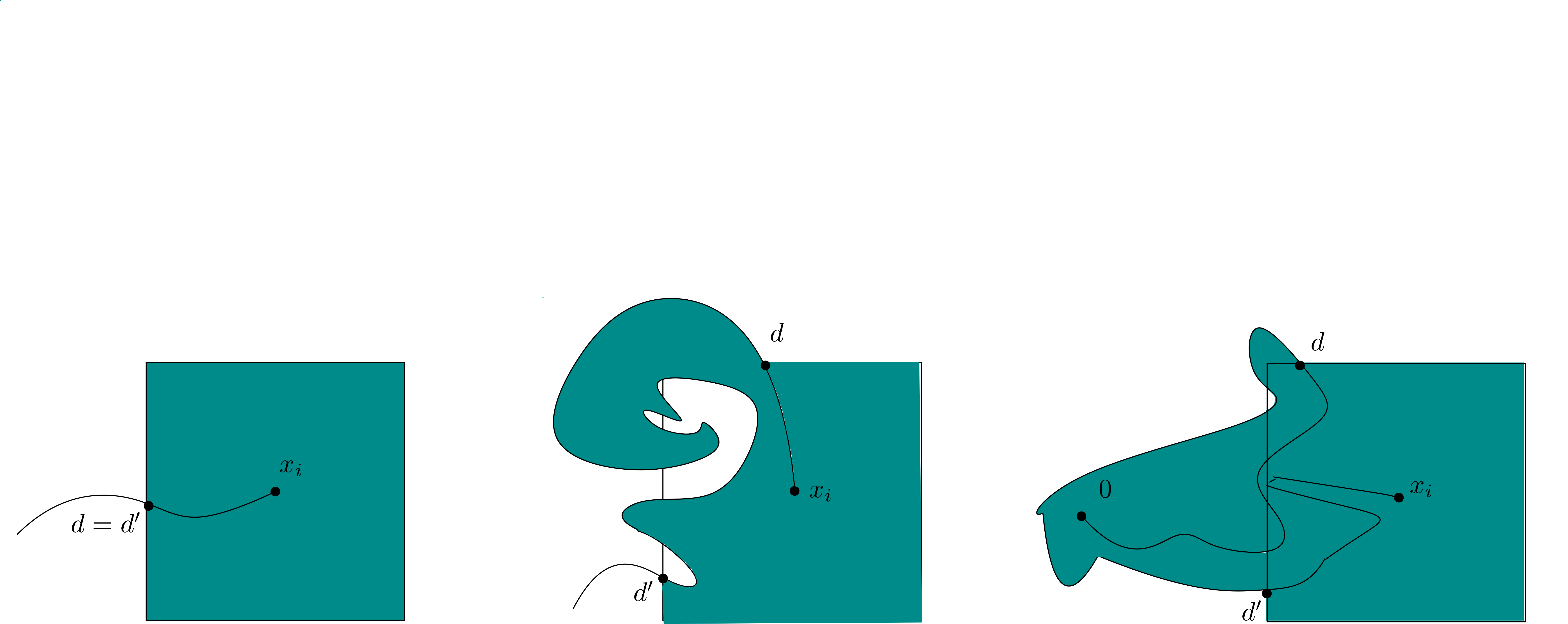
Figure 2: The explored backbone sketched in black together with the points $d$ and $d^{\prime}$ in three different cases. The domain $D_{i}$ coloured green. Note that in the first case $d=d^{\prime}$ and that in the last picture the position of $0$ is not to scale.  

Theorem 2.4.

Let $\Gamma\supset\{\mathrm{g},x\}$ be a set of vertices, $F$ be a set of edges, $\mathcal{Q}=\{F=\bar{\gamma}_{0,\Gamma}(\mathbf{n})\}$ and on the event $\mathcal{Q}$ let $\tilde{x}=\gamma_{0,\Gamma}^{\textit{end}}(\mathbf{n})$ be the unique vertex in $\Gamma$ connected to $x$ in $\gamma_{0,\Gamma}(\mathbf{n})$. Let $\mathcal{A}$ be an event such that $1_{\mathcal{A}}(\mathbf{n}_{\Lambda})1_{\mathcal{Q}}(\mathbf{n}_{\Lambda})=1_{\mathcal{A}}(\mathbf{n}_{\Lambda/F})1_{\mathcal{Q}}(\mathbf{n}_{F})$. Then whenever $\mathbb{P}^{\{0,x\}}_{\Lambda}(\mathcal{Q})>0$ it holds that

$$\mathbb{P}^{\{0,x\}}_{\Lambda}(\mathcal{A}\mid\mathcal{Q})=\mathbb{P}^{\{\tilde{x},x\}}_{\Lambda\backslash F}(\mathcal{A}).$$

Proof.

That $\mathbf{n}\in\mathcal{Q}$ means that the explored backbone of $\mathbf{n}$ up to $\Gamma$ is $F$. Thus, $F$ is the terminating set of the sequence $\{S_{i}\}_{i\in\mathbb{N}}$. Thus, on the event $\mathcal{Q}$ the current $\mathbf{n}$ restricted to $F$ must have sources $\partial\mathbf{n}_{F}=\{0\}\triangle\{u_{\text{end}}\} =\{0,\tilde{x}\}$. Since $\mathbf{n}=\mathbf{n}_{\Lambda\backslash F}+\mathbf{n}_{F}$ it holds that

$$\{0,x\}=\partial\mathbf{n}=\partial\mathbf{n}_{\Lambda\backslash F}\triangle\partial\mathbf{n}_{F}=\partial\mathbf{n}_{\Lambda\backslash F}\triangle\{0,\tilde{x}\}.$$

So for $\mathbf{n}\in\mathcal{Q}$ then $\partial\mathbf{n}_{\Lambda\backslash F}=\{\tilde{x},x\}.$ The map $\mathbf{n}\mapsto(\mathbf{n}_{F},\mathbf{n}_{\Lambda\backslash F})$ is a bijection from $\left\{\mathbf{n}\in\mathcal{Q}\mid\partial\mathbf{n}=\{0,x\}\right\}$ to $\left\{(\mathbf{n}_{F},\mathbf{n}_{\Lambda\backslash F})\mid\mathbf{n}_{F}+\mathbf{n}_{\Lambda\backslash F}\in\mathcal{Q},\partial\mathbf{n}_{F}=\{0,\tilde{x}\},\partial\mathbf{n}_{\Lambda\backslash F}=\{\tilde{x},x\}\right\}$ with inverse $(\mathbf{n}_{F},\mathbf{n}_{\Lambda\backslash F})\mapsto\mathbf{n}_{F}+\mathbf{n}_{\Lambda\backslash F}$. Thus, for any function $f:{\mathbb{N}_{0}}^{E\cup E_{\mathrm{g}}}\to\mathbb{R}$ it holds that

$$\sum_{\partial\mathbf{n}=\{0,x\}}f(\mathbf{n})1_{\mathcal{Q}}(\mathbf{n})=\sum_{\begin{subarray}{c}\partial\mathbf{n}_{F}=\{0,\tilde{x}\}\\  \partial\mathbf{n}_{\Lambda\backslash F}=\{\tilde{x},x\}\end{subarray}}f(\mathbf{n})1_{\mathcal{Q}}(\mathbf{n}).$$

Since $w(\mathbf{n}_{F}+\mathbf{n}_{\Lambda\backslash F})=w(\mathbf{n}_{F})\cdot w(\mathbf{n}_{\Lambda\backslash F})$ and the fact that $\mathcal{Q}$ only depends on edges in $F$, the double sum below factorizes and

$$\mathbb{P}^{\{0,x\}}_{\Lambda}(\mathcal{A}\mid\mathcal{Q}) =\frac{\sum_{\partial\mathbf{n}=\{0,x\}}w(\mathbf{n})1_{\mathcal{A}}(\mathbf{n})1_{\mathcal{Q}}(\mathbf{n})}{\sum_{\partial\mathbf{n}=\{0,x\}}w(\mathbf{n})1_{\mathcal{Q}}(\mathbf{n})}$$

$$=\frac{\sum_{\partial\mathbf{n}_{F}=\{0,\tilde{x}\},\partial\mathbf{n}_{\Lambda\backslash F}=\{\tilde{x},x\}}w(\mathbf{n}_{F}+\mathbf{n}_{\Lambda\backslash F})1_{\mathcal{A}}(\mathbf{n})1_{\mathcal{Q}}(\mathbf{n})}{\sum_{\partial\mathbf{n}_{F}=\{0,\tilde{x}\},\partial\mathbf{n}_{\Lambda\backslash F}=\{\tilde{x},x\}}w(\mathbf{n}_{F}+\mathbf{n}_{\Lambda\backslash F})1_{\mathcal{Q}}(\mathbf{n})}$$

$$=\frac{\sum_{\partial\mathbf{n}_{F}=\{0,\tilde{x}\}}w(\mathbf{n}_{F})1_{\mathcal{Q}}(\mathbf{n}_{F}) \sum_{\partial\mathbf{n}_{\Lambda\backslash F}=\{\tilde{x},x\}}w(\mathbf{n}_{\Lambda\backslash F})1_{\mathcal{A}}(\mathbf{n}_{\Lambda/F})}{\sum_{\partial\mathbf{n}_{F}=\{0,\tilde{x}\}}w(\mathbf{n}_{F})1_{\mathcal{Q}}(\mathbf{n}_{F})\sum_{\partial\mathbf{n}_{\Lambda\backslash F}=\{\tilde{x},x\}}w(\mathbf{n}_{\Lambda\backslash F})}$$

$$=\frac{\sum_{\partial\mathbf{n}_{\Lambda\backslash F}=\{\tilde{x},x\}}w(\mathbf{n}_{\Lambda\backslash F})1_{\mathcal{A}}(\mathbf{n}_{\Lambda\backslash F})}{\sum_{\partial\mathbf{n}_{\Lambda\backslash F}=\{\tilde{x},x\}}w(\mathbf{n}_{\Lambda\backslash F})}=\mathbb{P}^{\{\tilde{x},x\}}_{\Lambda\backslash F}(\mathcal{A}).$$

∎

[capbesideposition=left,top,capbesidewidth=4cm]figure[]

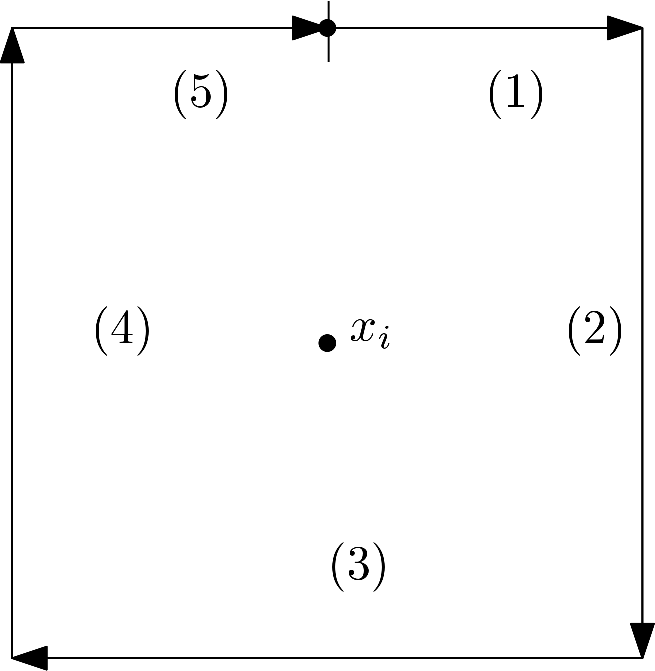
Figure 3: Sketch the order $\preceq$ on $\partial\Lambda_{1}(x_{i})$ used when defining $D_{i}$. Two points $a,b\in\partial\Lambda_{1}(x_{i})$ have $a\preceq b$ if the number of the segment of $a$ is smaller than the number of the segment of $b$ or if $a$ and $b$ are inside the same segment and $a$ is earlier than $b$ with respect to the arrow on that segment.

3 Main result

We now prove Theorem 1.2 given a result that we then prove later.

Before starting the proof, we go through some notation that we will use throughout the main section. Let $n$ be such that $x\in A_{9n,9(n+1)}$. In what follows, we will consider the case $\left|x\right| \geq 36$ which means that $n\geq 4$. In the proof of Theorem 1.2 we tie it together with the case $\left|x\right|<36$. We also let $\Lambda$ be any box which contains $\Lambda_{9(n+1)}$. Everything we prove will be independent of this $\Lambda$. Later we let $\Lambda\Uparrow\mathbb{Z}^{2}$.

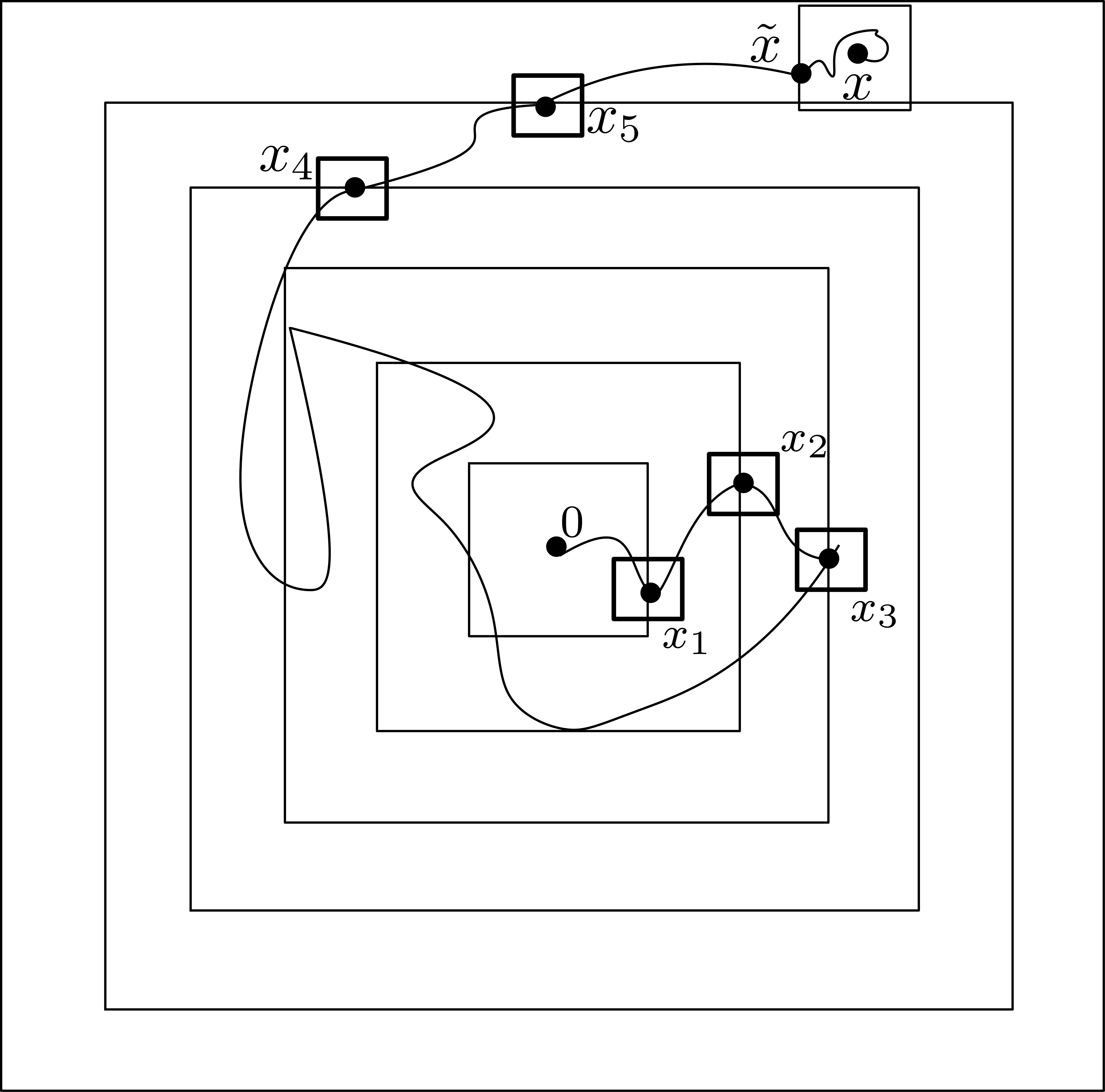
Figure 5: Sketch of the overall approach. Either the backbone goes through the ghost or we can define the $x_{i}$ as shown. Later, we show that it is probable that $x_{i}$ is connected to the ghost within each of the black squares.

We will explore the backbone partially in steps up to the annuli $A_{9i,9(i+1)}$. Suppose that in this exploration the backbone does not hit the ghost $\mathrm{g}$, which we can assume in our application. Then define $x_{i}=\gamma_{0,\Lambda_{9i}^{c}}^{\text{end}}(\mathbf{n}) \in A_{9i,9(i+1)}$. Thus, $x_{i}$ is random variable corresponding to the first vertex the backbone hits in the $i$-th annulus of the form $A_{9i,9(i+1)}$ see also Figure 5.

Further, to ease notation we let $\bar{\gamma}_{i}=\bar{\gamma}_{0,\Lambda_{9i}^{c}}(\mathbf{n})$. Thus, $\bar{\gamma}_{i}$ is the set of edges explored until the backbone hits the $i$-th annulus. Similarly, to ease notation let $\gamma_{i}=\gamma_{0,\Lambda_{9i}^{c}}(\mathbf{n})$. Thus, $\gamma_{i}$ is the path $u_{0},\dots,u_{\text{end}}=x_{i}=\gamma_{0,\Lambda_{9i}^{c}}^{\text{end}}(\mathbf{n})$ explored until the backbone hits the $i$-th annulus. Let $\mathcal{Q}_{\bar{\gamma}_{i}}$ be the event that the backbone explored is $\bar{\gamma}_{i}$.

A technical detail is that to account for removing the magnetic field in the box of size 1 around $x$ we explore the backbone partially also from $x$ until it leaves the box of size $2$. Denote the explored backbone $\bar{\gamma}_{x,\Lambda_{2}(x)^{c}}(\mathbf{n})$ by $\bar{\gamma}_{x}$, name the first point hit outside $\Lambda_{2}(x)$ by $\tilde{x}=\gamma_{x,\Lambda_{2}(x)^{c}}^{\text{end}}(\mathbf{n})$ and let the event that the explored backbone is $\bar{\gamma}_{x}$ be denoted $\mathcal{Q}_{\bar{\gamma}_{x}}$.

The set $\bar{\gamma}_{i}$ contains the path $\gamma_{i}$ from $0$ to $x_{i}$. Thus, $\bar{\gamma}_{i}$ will intersect $\partial\Lambda_{1}(x_{i})$ one or more times. Since $x_{i}$ is the first time the annulus $A_{9i,9(i+1)}$ is intersected the set $\bar{\gamma}_{i}\cap\partial\Lambda_{1}(x_{i})$ is contained within one half of $\partial\Lambda_{1}(x_{i})$. Let $d,d^{\prime}$ denote the points in $\bar{\gamma}_{i}\cap\partial\Lambda_{1}(x_{i})$ that are most clockwise and anticlockwise with respect to some way of walking around $\partial\Lambda_{1}(x_{i})$, see also Figure 2.

More formally, we consider an order $\preceq$ of the points in $\partial\Lambda_{1}(x_{i})$ and then define $d,d^{\prime}$ to be the minimal and maximal element of $\bar{\gamma}_{i}\cap\partial\Lambda_{1}(x_{i})$ with respect to this ordering. Let us define the order in the case where $x_{i}$ is in the right side of the annulus (which is the case $x_{1},x_{2},x_{3}$ on Figure 5) generalising to the other cases is straightforward. To do that, we split $\partial\Lambda_{1}(x_{i})$ and define the order with respect to the segments and arrows as shown on Figure 3.

Now, define $\Omega_{i}=\{v\in\partial\Lambda_{1}(x_{i})\mid d^{\prime}\preceq v\preceq d\}$ and let $\tilde{\Omega}_{i}=\partial\Lambda_{1}(x_{i})\backslash \Omega_{i}$. Let $\Sigma_{i}$ be the graph obtained by removing $\bar{\gamma}_{i}\cup\bar{\gamma}_{x}$ from $\Lambda$. Then we can define the domain $D_{i}$ to be the connected component of $x_{i}$ in the graph induced by the vertices of $\Sigma_{i}$ without $\tilde{\Omega}_{i}$. See also Figure 2. In the following claim we show how our order of exploration with respect to the incoming edge implies that $D_{i}$ is a bounded domain.

Claim 3.1.

The set $D_{i}\subset\Lambda_{9(i+1)}$ and it only depends on the current $\mathbf{n}_{\Lambda_{9i}}$.

Proof.

Since the vertex $d$ is explored by the backbone it is either on the backbone path $\gamma_{i}$ in which case we let $v=d$. Otherwise, there is an edge $e_{dv}$ from $d$ to a vertex on the backbone path that we call $v$. Similarly, we can define a vertex $v^{\prime}$ taking $d^{\prime}$ as the starting point. Let $P_{i}$ be the subpath of $\gamma_{i}$ which goes either from $v$ to $v^{\prime}$ or from $v^{\prime}$ to $v$ and extended by the edges $\{e_{dv}\}$ and/or $\{e^{\prime}_{d^{\prime}v^{\prime}}\}$ if $d,d^{\prime}$ are not on the backbone path. By construction the path $P_{i}$ is edge self-avoiding, but we do not know that $P_{i}$ is vertex self-avoiding and hence non self-intersecting. However, due to the way we explore the edges of the backbone with respect to the incoming edge if there is a vertex which is hit by the backbone path twice (i.e. $u_{i}=u_{j}$ for some $i\neq j$) then the backbone path must turn $90^{\circ}$ twice at that vertex. This means that we can deform the path slightly to be non-intersecting (see Figure 4).

Since $P_{i}$ is a path between $d$ and $d^{\prime}$ and further $\tilde{\Omega}_{i}$ is also a path between $d$ and $d^{\prime}$ along $\Lambda_{1}(x_{i})$ that by definition of $d$ and $d^{\prime}$, $P_{i}$ and $\tilde{\Omega}_{i}$ do not intersect. Thus, if we glue them together then $P_{i}\cup\tilde{\Omega}_{i}$ is a closed non-intersecting path, which therefore encloses a domain $Q_{i}$. Now, assume for contradiction that $\delta:x_{i}\to Q_{i}^{c}$ is a path. Since we have removed all the vertices in $\tilde{\Omega}_{i}$ including $d$ and $d^{\prime}$ it is impossible for $\delta$ to exit $Q_{i}$ through a vertex in $\tilde{\Omega}_{i}$. Since in the backbone exploration we remove the explored edges on the backbone path all remaining vertices have degree at most 2 in $\Sigma_{i}\backslash\tilde{\Omega}_{i}$. It is only possible to have a path exiting $Q_{i}$ if it crosses the path $P_{i}$ through a vertex of degree 2. The way we explore the backbone imply that if two edges remain they must have an angle of $90^{\circ}$. Therefore, the remaining edges do not cross $P_{i}$ and hence there is no such path $\delta$. Since $D_{i}$ is the connected component of $x_{i}$ it holds that $D_{i}\subset Q_{i}$ and boundedness of $D_{i}$ follows from boundedness of $Q_{i}$. ∎

[capbesideposition=left,top,capbesidewidth=8cm]figure[]

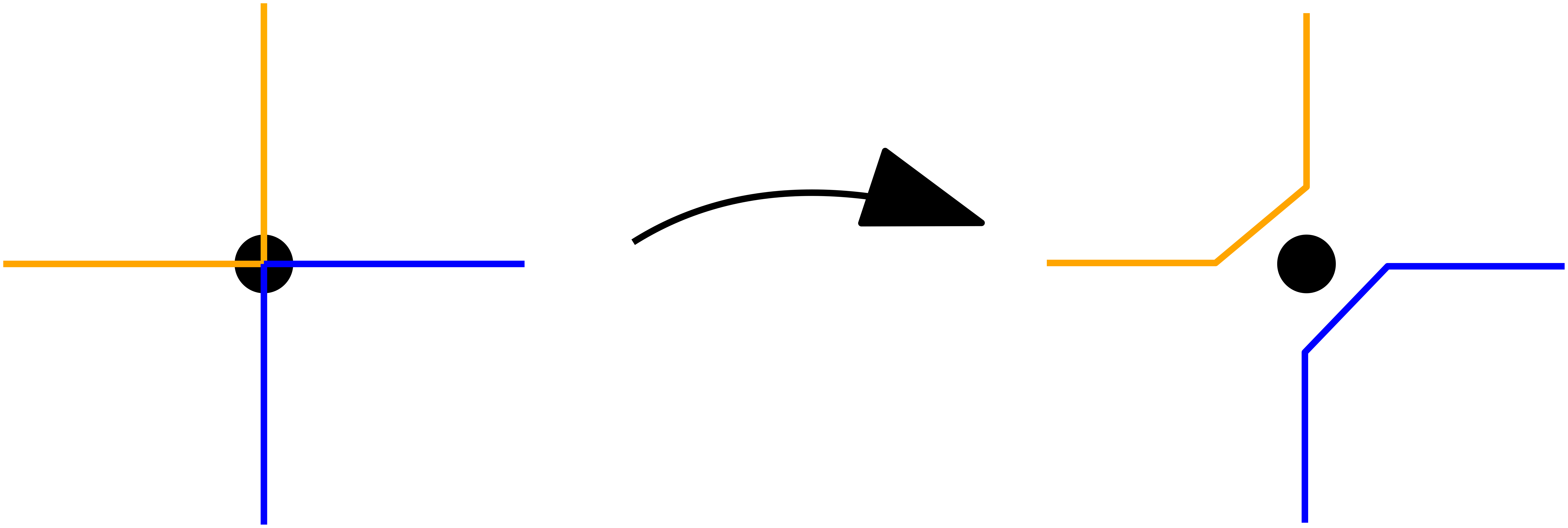
Figure 4: Sketch of the case where the backbone explores the same vertex twice as in the proof of Claim 3.1. Suppose that the backbone entered and left the vertex along edges of the same colour (orange or blue). Since we in the backbone exploration always explore turning to the right with respect to the incoming edge first the backbone path can never cross itself. Thus, a non-crossing deformation as shown is always possible.

To finish the setup we finally define

$$\mathcal{R}_{i}^{*}=\{\mathbf{n}\mid\partial\Lambda_{2}(x_{i})\overset{A_{2,4}(x_{i}) \backslash(D_{i}\cup\bar{\gamma}_{i})}{\not\leftrightarrow}\partial\Lambda_{4}(x_{i})\}.$$

Notice that if $\hat{\mathbf{n}}_{1}=\hat{\mathbf{n}}_{2}$ for two currents $\mathbf{n}_{1},\mathbf{n}_{2}$ and $\mathbf{n}_{1}\in\mathcal{R}_{i}^{*}$ then $\mathbf{n}_{2}\in\mathcal{R}_{i}^{*}$. Thus, $\mathcal{R}_{i}^{*}$ only depends on the traced and not on the full current. Define the corresponding connection event either for the traced current or for the random cluster measure by

$$\hat{\mathcal{R}}_{i}^{*}=\{\partial\Lambda_{2}(x_{i})\overset{A_{2,4}(x_{i}) \backslash(D_{i}\cup\bar{\gamma}_{i})}{\not\leftrightarrow}\partial\Lambda_{4}(x_{i})\}\subset\{0,1\}^{A_{2,4}(x_{i}) \backslash(D_{i}\cup\bar{\gamma}_{i})}.$$

Notice that $\hat{\mathcal{R}}_{i}^{*}=\left\{\hat{\mathbf{n}} \mid\mathbf{n}\in\mathcal{R}_{i}^{*}\right\}$. Hence, it holds that

$$\mathbb{P}^{\{x_{i},\tilde{x}\}}_{\Lambda\backslash(\bar{\gamma}_{i}\cup\bar{\gamma}_{x}),\vec{h}}\left(\mathcal{R}_{i}^{*}\right)=\hat{\mathbb{P}}^{\{x_{i},\tilde{x}\}}_{\Lambda\backslash(\bar{\gamma}_{i}\cup\bar{\gamma}_{x}),\vec{h}}\left(\hat{\mathcal{R}}_{i}^{*}\right).$$ (2)

The following proposition will yield the main result given Proposition 3.3 below. The idea of the proof is first to use the backbone exploration and then show that for every macroscopic step, with a strictly positive probability there is a connection to the ghost. To get the correct front factor $a^{\frac{1}{4}}$, we also partially explore the backbone also from the end around $x$ until $\tilde{x}=\gamma_{x,\Lambda_{2}(x)^{c}}^{\text{end}}(\mathbf{n})$.

Proposition 3.2.

Suppose that for all $\tilde{x}\in\partial\Lambda_{2}(x)$, all realisations of the backbone $\bar{\gamma}_{x}$ from $x$ to $\tilde{x}$, all $1\leq i\leq n$ and realisations of the backbone from $0$ to $x_{i}$ denoted $\bar{\gamma}_{i}$ and $a\leq 1$ that

$$\mathbb{P}^{\{x_{i},\tilde{x}\}}_{\Lambda\backslash(\bar{\gamma}_{i}\cup\bar{\gamma}_{x}),\vec{h}}\left(\mathcal{R}_{i}^{*}\right)\geq c$$

uniformly in any ($x$-dependent) $\Lambda$ sufficiently large. Then

$$\langle\sigma_{0};\sigma_{x}\rangle_{a,h}\leq Ca^{\frac{1}{4}}\exp\left(-M(h)\left|x\right|\right)$$

for $\left|x\right|\geq 36$ and where $M(h)$ does not depend on $a$.

Proof.

Let $\mathcal{H}$ be the event that the backbone explored from $0$ hits $x$ ( i.e. does not hit the ghost). Notice that $\{\tilde{x}=\mathrm{g}\} \cap\mathcal{Q}_{\bar{\gamma}_{x}}\cap\mathcal{H}=\emptyset$ so when we condition $\mathcal{H}$ on all possible events $\mathcal{Q}_{\bar{\gamma}_{x}}$ we can omit those where $\tilde{x}=\mathrm{g}$. In other words, if $\tilde{x}=\mathrm{g}$ then the backbone explored from $0$ would necessarily hit the ghost since after the partial backbone exploration then $\mathrm{g}$ and $0$ would be the only two vertices with odd degree.

Further, $1_{\mathcal{H}}(\mathbf{n}_{\Lambda})1_{\mathcal{Q}_{\bar{\gamma}_{x}}}(\mathbf{n}_{\Lambda})=1_{\mathcal{H}}(\mathbf{n}_{\Lambda\backslash\bar{\gamma}_{x}})1_{\mathcal{Q}_{\bar{\gamma}_{x}}}(\mathbf{n}_{\bar{\gamma}_{x}})$  so by the backbone exploration Theorem 2.4

$$\mathbb{P}^{\{0,x\}}_{\Lambda,\vec{h}}(\mathcal{H})=\sum_{\bar{\gamma}_{x}}\mathbb{P}^{\{0,x\}}_{\Lambda,\vec{h}}(\mathcal{H}\mid\mathcal{Q}_{\bar{\gamma}_{x}})\mathbb{P}^{\{0,x\}}_{\Lambda,\vec{h}}(\mathcal{Q}_{\bar{\gamma}_{x}})=\sum_{\bar{\gamma}_{x}}\mathbb{P}^{\{0,\tilde{x}\}}_{\Lambda\backslash\bar{\gamma}_{x},\vec{h}}(\mathcal{H})\mathbb{P}^{\{0,x\}}_{\Lambda,\vec{h}}(\mathcal{Q}_{\bar{\gamma}_{x}})$$ (3)

where we from now on assume that $\tilde{x}\neq\mathrm{g}$ which means that $\tilde{x}\in\partial\Lambda_{2}(x)$.

For each $1\leq i\leq n$ let $\mathcal{G}_{i}$ be the event that the backbone hits the annulus $A_{9i,9(i+1)}$ before hitting the ghost. Given a current configuration in $\mathcal{G}_{i}$ we know that the vertices $x_{j}$ exist for $1\leq j\leq i$. Further, if we define $\mathcal{G}_{0}=\left\{\mathbf{n}\mid\partial\mathbf{n}=\{0,x\}\right\}$ then $\mathcal{G}_{i+1}\subset\mathcal{G}_{i}$ for each $0\leq i\leq n-1$ as well as $\{0\not\leftrightarrow\mathrm{g}\} \subset\mathcal{H}\subset\mathcal{G}_{n}$. Since $\mathbb{P}^{\{0,\tilde{x}\}}_{\Lambda\backslash\bar{\gamma}_{x},\vec{h}}(\mathcal{H})\leq\mathbb{P}^{\{0,\tilde{x}\}}_{\Lambda\backslash\bar{\gamma}_{x},\vec{h}}(\mathcal{G}_{n})$ and bounding $\mathbb{P}^{\{0,\tilde{x}\}}_{\Lambda\backslash\bar{\gamma}_{x},\vec{h}}(\mathcal{H})$ uniformly in $\bar{\gamma}_{x}$ bounds $\mathbb{P}^{\{0,x\}}_{\Lambda,\vec{h}}\left(\mathcal{H}\right)$ through (3). It means that to bound $\mathbb{P}^{\{0,x\}}_{\Lambda,\vec{h}}(0\not\leftrightarrow\mathrm{g})$ it suffices to show exponential decay of $\mathbb{P}^{\{0,\tilde{x}\}}_{\Lambda\backslash\bar{\gamma}_{x},\vec{h}}(\mathcal{G}_{n})$ uniformly in $\bar{\gamma}_{x}$. Notice that given $\mathcal{Q}_{\bar{\gamma}_{i-1}}$ then $\mathcal{G}_{i}$ depends only on edges in $\Lambda\backslash(\bar{\gamma}_{i-1}\cup\bar{\gamma}_{x})$ so

$$1_{\mathcal{G}_{i}}(\mathbf{n}_{\Lambda\backslash\bar{\gamma}_{x}})1_{\mathcal{Q}_{\bar{\gamma}_{i-1}}}(\mathbf{n}_{\Lambda\backslash\bar{\gamma}_{x}})=1_{\mathcal{G}_{i}}(\mathbf{n}_{\Lambda\backslash(\bar{\gamma}_{i-1}\cup\bar{\gamma}_{x})})1_{\mathcal{Q}_{\bar{\gamma}_{i-1}}}(\mathbf{n}_{(\bar{\gamma}_{i-1}\cup\bar{\gamma}_{x})})$$

and by the backbone exploration Theorem 2.4

$$\mathbb{P}_{\Lambda\backslash\bar{\gamma}_{x},\vec{h}}^{\{0,\tilde{x}\}}(\mathcal{G}_{n}) =\left[\prod_{i=1}^{n}\mathbb{P}_{\Lambda\backslash\bar{\gamma}_{x},\vec{h}}^{\{0,\tilde{x}\}}(\mathcal{G}_{i}\mid\mathcal{G}_{i-1})\right]\mathbb{P}_{\Lambda\backslash\bar{\gamma}_{x},\vec{h}}^{\{0,\tilde{x}\}}(\mathcal{G}_{0})$$

$$=\prod_{i=1}^{n}\sum_{\mathcal{Q}_{\bar{\gamma}_{i-1}}\in\mathcal{G}_{i-1}}\mathbb{P}_{\Lambda\backslash\bar{\gamma}_{x},\vec{h}}^{\{0,\tilde{x}\}}(\mathcal{G}_{i}\mid\mathcal{Q}_{\bar{\gamma}_{i-1}})\mathbb{P}_{\Lambda\backslash\bar{\gamma}_{x},\vec{h}}^{\{0,\tilde{x}\}}(\mathcal{Q}_{\bar{\gamma}_{i-1}}\mid\mathcal{G}_{i-1})$$

$$\leq\prod_{i=1}^{n}\sum_{\mathcal{Q}_{\bar{\gamma}_{i-1}}\in\mathcal{G}_{i-1}}\mathbb{P}_{\Lambda\backslash(\bar{\gamma}_{i-1}\cup\bar{\gamma}_{x}),\vec{h}}^{\{x_{i-1},\tilde{x}\}}(\mathcal{G}_{i})\mathbb{P}_{\Lambda\backslash\bar{\gamma}_{x},\vec{h}}^{\{0,\tilde{x}\}}(\mathcal{Q}_{\bar{\gamma}_{i-1}}\mid\mathcal{G}_{i-1})\leq(1-c)^{n-2}$$

where in the last step we used $\mathbb{P}_{\Lambda\backslash(\bar{\gamma}_{i-1}\cup\bar{\gamma}_{x}),\vec{h}}^{\{x_{i-1},\tilde{x}\}}(\mathcal{G}_{i})\leq\mathbb{P}_{\Lambda\backslash(\bar{\gamma}_{i-1}\cup\bar{\gamma}_{x}),\vec{h}}^{\{x_{i-1},\tilde{x}\}}({\mathcal{R}^{*c}_{i-1}})\leq 1-c$. Now, by the remarks in the beginning of the proof it follows from Proposition 2.1 that

$$\langle\sigma_{0};\sigma_{x}\rangle_{\Lambda,h,a}\leq Ca^{\frac{1}{4}}\mathbb{P}^{\{0,x\}}_{\Lambda,\vec{h}}\left(0\not\leftrightarrow\mathrm{g}\right)\leq Ca^{\frac{1}{4}}(1-c)^{n-2}=Ca^{\frac{1}{4}}\exp(-M(h)\left|x\right|).$$

The inequality passes to the infinite volume limit since the constants are independent of $\Lambda$. ∎

[capbesideposition=left,top,capbesidewidth=4cm]figure[]

Next, we will move from the random current event $\mathcal{R}_{i}^{*}$ to the traced current or random cluster event $\hat{\mathcal{R}}_{i}^{*}$. In the remaining section we will prove the following proposition which only concerns the random cluster model. Here and in all of the following by $\geq c$ we mean larger than a (possibly different each time) strictly positive constant which is uniform in $a\leq 1$, $h$ and the explored backbones $\bar{\gamma}_{i}$ and $\bar{\gamma}_{x}$ .

Proposition 3.3.

There is a $h_{0}>0$ such that for all realisations of the backbone $\bar{\gamma}_{i}$ up to $x_{i}$, all $\bar{\gamma}_{x}$ explored until $\tilde{x}\in\partial\Lambda_{2}(x)$ and all $a\leq 1,h<h_{0}$ then

$$\phi^{0,a}_{\Lambda\backslash(\bar{\gamma}_{i}\cup\bar{\gamma}_{x}),\vec{h}}\left(\hat{\mathcal{R}}_{i}^{*}\mid x_{i}\leftrightarrow\tilde{x}\right)\geq c$$

uniformly in any $\Lambda$ sufficiently large around $x$.

Now, collecting the results we can prove the main theorem assuming Proposition 3.3 which is in the language of the random cluster model where many more tools are available than for random currents most notably the RSW.

Proof of Theorem 1.2.

By (2), the monotone coupling from Theorem 2.3 along with the fact that $\hat{\mathcal{R}}_{i}^{*}$ is a decreasing event and Proposition 3.3 we get that

$$\mathbb{P}^{\{x_{i},\tilde{x}\}}_{\Lambda\backslash(\bar{\gamma}_{i}\cup\bar{\gamma}_{x}),\vec{h}}\left(\mathcal{R}_{i}^{*}\right)=\mathbb{P}^{\{x_{i},\tilde{x}\}}_{\Lambda\backslash(\bar{\gamma}_{i}\cup\bar{\gamma}_{x}),\vec{h}}(\hat{\mathcal{R}}_{i}^{*})\geq\phi^{0,a}_{\Lambda\backslash(\bar{\gamma}_{i}\cup\bar{\gamma}_{x}),\vec{h}}\left(\hat{\mathcal{R}}_{i}^{*}\mid x_{i}\leftrightarrow\tilde{x}\right)\geq c.$$

Thus, we can apply Proposition 3.2. In Proposition 3.3 we only have the result for sufficiently small $h$, but this suffices by the GHS-inequality [36]. To account for the constraint $\left|x\right|\geq 36$ in Proposition 3.2 and get the correct front factor notice that from the GHS inequality and Proposition 5.5 in [37] some $B>0$ it holds for all $x\in a\mathbb{Z}^{2}$ that

$$\langle\sigma_{0};\sigma_{x}\rangle_{a,h}\leq\langle\sigma_{0};\sigma_{x}\rangle_{a,0}\leq B\left(\frac{a}{\left|x\right|}\right)^{\frac{1}{4}}.$$

Using that for $\left|x\right| \geq K(h)$ it holds that

$$\langle\sigma_{0};\sigma_{x}\rangle_{a,h}\leq Ca^{\frac{1}{4}}\exp\left(-\frac{M(h)}{2}\left|x\right|\right)\exp\left(-\frac{M(h)}{2}\left|x\right|\right)\leq C\left(\frac{a}{\left|x\right|}\right)^{\frac{1}{4}}\exp\left(-\frac{M(h)}{2}\left|x\right|\right).$$

By putting $C(h)=\max\{B,C\} \exp\left(\frac{M(h)}{2}K(h)\right)$ and $m(h)=\frac{M(h)}{2}$ our main result Theorem 1.2 follows.

∎

4 Proof of Proposition 3.3

Recall that $\Sigma_{i}=\Lambda\backslash(\bar{\gamma}_{i}\cup\bar{\gamma}_{x})$. To ease the notation here and in what follows we define $\phi_{\Sigma_{i}}=\phi^{0,a}_{\Sigma_{i},\vec{h}}=\phi^{0,a}_{\Lambda\backslash(\bar{\gamma}_{i}\cup\bar{\gamma}_{x}),\vec{h}}$. Further, for a set $\Gamma$ let $x\overset{\Gamma^{+}}{\leftrightarrow}y$ denote the event that $x$ and $y$ are connected in $\Gamma\cup\{\mathrm{g}\}$ and similarly by $x\overset{\Gamma}{\leftrightarrow}y$ that $x$ and $y$ are connected in $\Gamma$ not using the ghost. Define the domain $T_{i}$ to be all points in $D_{i}$ as well as all points in $\Lambda_{2}(x_{i})$ that can be reached from $x_{i}$ without using edges in $\bar{\gamma}_{i}$ or $\partial\Lambda_{2}(x_{i})$. Further, define $\{x_{i}\overset{T_{i}^{+}}{\leftrightarrow}\mathrm{g}\}$ to be the event that $x_{i}$ is connected within the domain $T_{i}$ to some vertex $v$ where the edge from $v$ to $\mathrm{g}$ is open. Define $\tilde{D}$ and $\tilde{T}$ similarly to $D_{i}$ and $T_{i}$ with $\tilde{x}$ instead of $x_{i}$. Define also $A_{i}=\partial\Lambda_{2}(x_{i})\cap T_{i}^{c}$ and $\tilde{A}=\partial\Lambda_{2}(\tilde{x})\cap\tilde{T}^{c}$.

Proposition 4.1.

Suppose for some $1<i<n$ that $\phi_{\Sigma_{i}}\left(x_{i}\overset{T_{i}^{+}}{\leftrightarrow}\mathrm{g}\mid x_{i}\leftrightarrow A_{i}\right)\geq c$
and $\phi_{\Sigma_{i}}\left(\tilde{x}\overset{\tilde{T}^{+}}{\leftrightarrow}\mathrm{g}\mid\tilde{x}\leftrightarrow\tilde{A}\right)\geq c$. Then for all $h\leq h_{0}$ it holds that $\phi_{\Sigma_{i}}\left(\hat{\mathcal{R}}_{i}^{*}\mid x_{i}\leftrightarrow\tilde{x}\right)\geq c.$

We first state the recent result that the random cluster model still has the RSW property at scales up to the correlation length. Here we need the wired boundary condition which is introduced in for example [7].

Lemma 4.2.

([3], Lemma 8.5) For any sufficiently large $C>0$, there is an $\varepsilon>0$ such that if $n\geq 1$ and $H\geq 0$ are such that $Hn^{2}\phi_{\Lambda_{n},H=0}^{0,a=1}(0\leftrightarrow\partial\Lambda_{n})\leq\varepsilon$ then

$$\phi_{A_{n,2n},H=0}^{1,a=1}(\Lambda_{n}\not\leftrightarrow\partial\Lambda_{2n})\leq C\phi_{A_{n,2n},H}^{1,a=1}(\Lambda_{n}\not\leftrightarrow\partial\Lambda_{2n}).$$

Translating the lemma into our setting yields the following lemma.

Lemma 4.3.

There exists a $h_{0}>0$ such that for $a\leq 1$ and $h\leq h_{0}$ it holds that

$$\phi^{0}_{\Sigma_{i},\vec{h}}(\hat{\mathcal{R}}_{i}^{*})\geq c.$$

where $c>0$ is (as always) independent of $0<a\leq 1,\Sigma_{i}$ and $0\leq h<h_{0}$. Further, for any event $E$ depending only on edges in $D_{i}$ it holds that

$$\phi_{\Sigma_{i}}^{0}(\hat{\mathcal{R}}_{i}^{*}\mid E)\geq c.$$

Proof.

If $n=\frac{2}{a}$ and $H=a^{\frac{15}{8}}h$ then using equation (1-arm)

$$Hn^{2}\phi_{\Lambda_{n},H=0}^{0,a=1}(0\leftrightarrow\partial\Lambda_{n})\leq C(an)^{\frac{15}{8}}h=C2^{\frac{15}{8}}h\leq\varepsilon$$

which can be satisfied by choosing $h$ sufficiently small (independent of $a$). Therefore

$$\phi_{A_{2,4},h}^{1,a}(\Lambda_{2}\not\leftrightarrow\partial\Lambda_{4})=\phi_{A_{\frac{2}{a},\frac{4}{a}},ha^{\frac{15}{8}}}^{1,1}(A_{\frac{2}{a}}\not\leftrightarrow\partial A_{\frac{4}{a}})\geq C\phi_{A_{\frac{2}{a},\frac{4}{a}},h=0}^{1,1}(A_{\frac{2}{a}}\not\leftrightarrow\partial A_{\frac{4}{a}})=C\phi_{A_{2,4},h=0}^{1,a}(\Lambda_{2}\not\leftrightarrow\partial\Lambda_{4}).$$

Since $\hat{\mathcal{R}}_{i}^{*}$ is decreasing it follows by (MON) and the RSW for usual rectangles [37] that

$$\phi^{0,a}_{\Sigma_{i},\vec{h}}(\hat{\mathcal{R}}_{i}^{*}) \geq\phi^{0,a}_{\Sigma_{i},h}(\hat{\mathcal{R}}_{i}^{*})\geq\phi^{0,a}_{\Lambda,h}(\hat{\mathcal{R}}_{i}^{*})\geq\phi^{0,a}_{\Lambda,h}(\Lambda_{2}(x_{i})\not\leftrightarrow\partial\Lambda_{4}(x_{i}))\geq\phi_{\Lambda,h}^{1,a}(\Lambda_{2}(x_{i})\not\leftrightarrow\partial\Lambda_{4}(x_{i}))$$

$$\geq\phi_{A_{2,4},h}^{1,a}(\Lambda_{2}\not\leftrightarrow\partial\Lambda_{4})\geq c\phi_{A_{2,4},h=0}^{1,a}(\Lambda_{2}\not\leftrightarrow\partial\Lambda_{4})\geq c.$$

Using comparison between boundary conditions, and that because of the argument in Claim 3.1 removing all explored edges of the backbone acts as a free boundary condition it holds that

$$\phi^{0}_{\Sigma_{i},\vec{h}}(\hat{\mathcal{R}}_{i}^{*}\mid E)\geq\phi^{1\text{ on }\partial\Lambda_{1}(x_{i}),0 \text{else}}_{\Sigma_{i}\backslash D_{i},h}(\hat{\mathcal{R}}_{i}^{*})\geq\phi_{A_{2,4},h}^{1,a}(\Lambda_{2}\not\leftrightarrow\partial\Lambda_{4})\geq c.$$

∎

Next, we need the general result that we can do mixing also with a magnetic field at scales up to the correlation length and that we, up to constants, can decorrelate events in $T_{i}$ from events in $(T_{i}\cup\Lambda_{4}(x_{i}))^{c}$. Define $J_{i}=(T_{i}\cup\Lambda_{4}(x_{i}))\backslash\bar{\gamma}_{i}$ and $\tilde{J}=(\tilde{T}\cup\Lambda_{4}(\tilde{x}))\backslash\bar{\gamma}_{x}$. Define also $\hat{\mathcal{R}}^{*}_{\sim}$ similarly to $\hat{\mathcal{R}}^{*}_{i}$ as an event in the vicinity of $\tilde{x}$ instead of $x_{i}$.

Lemma 4.4.

(Mixing) Let $E_{1},E_{2}$ be increasing events that only depend on edges in the boxes $T_{i}\cup\Lambda_{2}(x_{i})$ and $\tilde{T}\cup\Lambda_{2}(\tilde{x})$ respectively. Then for $1\leq i\leq n-2$ it holds that

$$\phi^{0}_{\Sigma_{i}}(E_{1}\cap E_{2})\asymp\phi^{0,a}_{J_{i},\vec{h}}(E_{1})\phi^{0,a}_{\tilde{J},\vec{h}}(E_{2})$$

Similarly, if $l\leq 1$, $z_{1},z_{2}$ are such that $\Lambda_{2l}(z_{1})\cap\Lambda_{2l}(z_{2})=\emptyset$ and $E_{1},E_{2}$ are increasing events that only depend on edges in the boxes $\Lambda_{l}(z_{1}),\Lambda_{l}(z_{2})$ respectively. Then

$$\phi^{0}_{\Sigma_{i}}(E_{1}\cap E_{2})\asymp\phi^{0,a}_{\Lambda_{2l}(z_{1})\backslash(\bar{\gamma}_{i}\cup\bar{\gamma}_{x}),\vec{h}}(E_{1})\phi^{0,a}_{\Lambda_{2l}(z_{2})\backslash(\bar{\gamma}_{i}\cup\bar{\gamma}_{x}),\vec{h}}(E_{2}).$$

Proof.

We prove the first statement first. Define $E=E_{1}\cap E_{2}$. It follows from Lemma 4.3 that

$$c\phi^{0}_{\Sigma_{i}}(E)\leq\phi_{\Sigma_{i}}(E\mid\hat{\mathcal{R}}_{i}^{*})$$

and similarly we can condition on $\hat{\mathcal{R}}^{*}_{\sim}$. Using that closed dual paths inside the annulus give rise to monotonicity properties as free boundary conditions (which is for example proven in Lemma 11 in [1]) we obtain that

$$c\phi^{0}_{\Sigma_{i}}(E) \leq\phi_{\Sigma_{i}}(E_{1},E_{2}\mid\hat{\mathcal{R}}_{i}^{*},\hat{\mathcal{R}}^{*}_{\sim})\leq\phi^{0}_{J_{i}\cup\tilde{J},\vec{h}}(E_{1},E_{2})=\phi^{0}_{J_{i},\vec{h}}(E_{1})\phi^{0}_{\tilde{J},\vec{h}}(E_{2}).$$

Since the reverse inequality is (FKG) and (MON) the first result follows. The second assertion follows mutatis mutandis using that the estimates from the proof of Lemma 4.3 which by Lemma 4.2 also work on smaller scales and using the event $\{\partial\Lambda_{l}(z_{i})\not\leftrightarrow\partial\Lambda_{2l}(z_{i})\}$ for $i=1,2$ instead of $\hat{\mathcal{R}}_{i}^{*}$ and $\hat{\mathcal{R}}^{*}_{\sim}$. ∎

With the lemmas proven we continue to the proof of the Proposition 4.1.

Proof of Proposition 4.1.

First, notice that

$$\phi_{\Sigma_{i}}\left(\hat{\mathcal{R}}_{i}^{*}\mid x_{i}\overset{\Sigma_{i}^{+}}{\leftrightarrow}\tilde{x}\right)\geq\phi_{\Sigma_{i}}\left(\hat{\mathcal{R}}_{i}^{*}\mid x_{i}\overset{T_{i}}{\leftrightarrow}\mathrm{g},\tilde{x}\overset{\tilde{T}}{\leftrightarrow}\mathrm{g}\right)\phi_{\Sigma_{i}}\left(x_{i}\overset{T_{i}}{\leftrightarrow}\mathrm{g},\tilde{x}\overset{\tilde{T}}{\leftrightarrow}\mathrm{g}\mid x_{i}\overset{\Sigma_{i}^{+}}{\leftrightarrow}\tilde{x}\right).$$

From the mixing argument in Lemma 4.3 it follows that $\phi_{\Sigma_{i}}\left(\hat{\mathcal{R}}_{i}^{*}\mid x_{i}\overset{T_{i}}{\leftrightarrow}\mathrm{g},\tilde{x}\overset{\tilde{T}}{\leftrightarrow}\mathrm{g}\right)\geq c$. Thus, we just need to prove that $\phi_{\Sigma_{i}}\left(x_{i}\overset{T_{i}}{\leftrightarrow}\mathrm{g},\tilde{x}\overset{\tilde{T}}{\leftrightarrow}\mathrm{g}\right)\geq c\phi_{\Sigma_{i}}\left(x_{i}\overset{\Sigma_{i}^{+}}{\leftrightarrow}\tilde{x}\right).$ Notice that

$$\{x_{i}\overset{\Sigma_{i}^{+}}{\leftrightarrow}\tilde{x}\}\subset\left(\{x_{i}\overset{T_{i}}{\leftrightarrow}\mathrm{g}\}\cup\{x_{i}\leftrightarrow A_{i}\}\right)\cap\left(\{\tilde{x}\overset{\tilde{T}}{\leftrightarrow}\mathrm{g}\}\cup\{\tilde{x}\leftrightarrow\tilde{A}\}\right).$$

Now, by first a union bound, then (Mixing) and the assumption and finally (MON) and (FKG)

$$\phi_{\Sigma_{i}}\left(x_{i}\overset{\Sigma_{i}^{+}}{\leftrightarrow}\tilde{x}\right) \leq\phi_{\Sigma_{i}}\left(x_{i}\overset{T_{i}}{\leftrightarrow}\mathrm{g},\tilde{x}\overset{\tilde{T}}{\leftrightarrow}\mathrm{g}\right)+\phi_{\Sigma_{i}}\left(x_{i}\overset{T_{i}}{\leftrightarrow}\mathrm{g},\tilde{x}\leftrightarrow\tilde{A}\right)$$

$$+\phi_{\Sigma_{i}}\left(x_{i}\leftrightarrow A_{i},\tilde{x}\overset{\tilde{T}}{\leftrightarrow}\mathrm{g}\right)+\phi_{\Sigma_{i}}\left(x_{i}\leftrightarrow A_{i},\tilde{x}\leftrightarrow\tilde{A}\right)$$

$$\leq 4C\phi^{0,a}_{J_{i},\vec{h}}\left(x_{i}\overset{T_{i}}{\leftrightarrow}\mathrm{g}\right)\phi^{0,a}_{\tilde{J},\vec{h}}\left(\tilde{x}\overset{\tilde{T}}{\leftrightarrow}\mathrm{g}\right)\leq c\phi_{\Sigma_{i}}\left(x_{i}\overset{T_{i}}{\leftrightarrow}\mathrm{g},\tilde{x}\overset{\tilde{T}}{\leftrightarrow}\mathrm{g}\right).$$

∎

We now turn to the main technical part for proving Proposition 3.3. From now on, we will assume, for notational reasons, without loss of generality that $x_{i}$ is on the right side of the inner boundary of the annulus $A_{9i,9(i+1)}$, i.e. that $x_{i}=(\frac{9i}{2},y)$ for some $y$ such that $-\frac{9i}{2}\leq y\leq\frac{9i}{2}$. Then define $L=[1,2]\times[0,\frac{1}{10}]+x_{i}$ and $\tilde{L}$ similarly to be a rectangle in the vicinity of $\tilde{x}$.

Lemma 4.5.

For each $1<i<n$ it holds that

$$\phi^{0}_{\Sigma_{i}}(x_{i}\leftrightarrow L\mid x_{i}\leftrightarrow A_{i})\geq c\text{ as well as } \phi^{0}_{\Sigma_{i}}(\tilde{x}\leftrightarrow L\mid \tilde{x}\leftrightarrow\tilde{A})\geq c.$$

Let $C(x_{i})$ be number of points in $\Lambda_{2}(x_{i})$ connected to $x_{i}$ without using edges to the ghost and $N_{M,i}=\{C(x_{i})\geq M\}$ for each $M\in\mathbb{N}$.

Lemma 4.6.

Let $k>0$. Then,

$$\phi^{0}_{\Sigma_{i}}\left(N_{ka^{-\frac{15}{8}},i}\mid x_{i}\leftrightarrow L,x_{i}\leftrightarrow A_{i}\right)\geq c.$$

Then let us start proving the lemmas. To do that we need to show that crossings of topological rectangles exist with constant probability. This is done in ([38], Theorem 1.1) if the discrete extremal length $l_{\Omega}[(ab),(cd)]$ is bounded. From ([38],(3.7)) (see also [39]) we have the following characterisation of the discrete extremal length

$$l_{\Omega}((ab),(cd))=\sup_{g:E(\Omega)\to\mathbb{R}_{+}\cup\{0\}}\frac{\left(\inf_{\gamma:(ab)\leftrightarrow(cd)}\sum_{e\in\gamma}g_{e}\right)^{2}}{\sum_{e}g_{e}^{2}}$$

where the supremum is over all non-negative, not identically zero functions on the edges. Using this representation we obtain the following lemma (which is equivalent to Rayleigh’s monotonicity law) .

Lemma 4.7.

Let $T$ be a topological rectangles with marked points $(abcd)$. Let $e,f$ be points on $(ad)$ and $\gamma$ a path from $e$ to $f$ inside $T$. Let $\tilde{T}$ be the points in $T$ reachable from $b$ in $T\backslash\gamma$. Note $\tilde{T}$ is a new topological rectangle with marked points $(abcd)$. Then,

$$l_{T}\left((ad),(bc)\right)\geq l_{\tilde{T}}\left((ad),(bc)\right) l_{T}\left((ab),(cd)\right)\geq l_{\tilde{T}}\left((ab),(cd)\right).$$ as well as

Proof.

We prove the first inequality, the second follows similarly. Since the graph $\tilde{T}$ is finite the supremum and infimum are attained and we get some maximizing function $\tilde{g}$ for $\tilde{T}$. Now, define the function $g$ by extending $\tilde{g}$ with $g(e)=0$ whenever $e\not\in T\backslash\tilde{T}$. Then,

$$l_{\tilde{T}}((ad)\leftrightarrow(bc))=\frac{\left(\inf_{\gamma:(ad)\leftrightarrow(bc)\text{ in }\tilde{T}}\sum_{e\in\gamma}\tilde{g}_{e}\right)^{2}}{\sum_{e}\tilde{g}_{e}^{2}}=\frac{\left(\inf_{\gamma:(ad)\leftrightarrow(bc)\text{ in }T}\sum_{e\in\gamma}g_{e}\right)^{2}}{\sum_{e}g_{e}^{2}}\leq l_{T}((ad)\leftrightarrow(bc)).$$

The second equality follows since any path $\gamma:(ad)\leftrightarrow(bc)\text{ in }T$ has a subpath $\tilde{\gamma}:(ad)\leftrightarrow(bc)\text{ in }\tilde{T}$. The inequality follows since the function $g$ is just one element in the supremum defining the discrete extremal length. ∎

Using Lemma 4.7 we can now prove Lemma 4.5

Proof of Lemma 4.5.

Define the explored vertices $\mathcal{V}$ of the backbone to be all vertices with at least one incident explored edge. Then define $U$ to be the set of vertices in $V(\Lambda)\backslash(\mathcal{V}\cup D_{i})$ with at least one edge to $\mathcal{V}$. Since $\gamma_{i}\cap\Lambda_{2,R}(x_{i})=\emptyset$ there exists at least one $*$-path (i.e. a path that can also jump diagonally) ${P_{i}}^{*}$ in $U$ from $d$ to a vertex in $\partial\Lambda_{2}^{c}(x_{i})$. From such a $*$-path $P_{i}^{*}$ we can construct a usual path $P_{i}$ just going around the plaquette every time ${P_{i}}^{*}$ jumps diagonally. Let the first vertex that $P_{i}$ hits in $\Lambda_{2}(x_{i})^{c}$ be $d_{1}$ and denote henceforth the path $P_{i}$ by $(dd_{1})$. Define $d_{1}^{\prime}$ similarly following the outside of the backbone from $d^{\prime}$.

Now, let $\Lambda_{1}(x_{i})_{R}$ denote the right half of the box $\Lambda_{1}(x_{i})$. Define $a_{i}=x_{i}+(1,-1)$, $b_{i}=x_{i}+(2,-1)$, $a_{i}^{\prime}=x_{i}^{\prime}+(1,1)$ and $b_{i}^{\prime}=x_{i}+(2,1)$ see Figure 6. Define $T_{i,1}=\Lambda_{2}(x_{i})\backslash D_{i}$. Then let $\mathcal{S}_{i}\in\{0,1\}^{E(T_{i,1})}$ be the event defined by

$$\mathcal{S}_{i}=\left\{ (a_{i}b_{i})\overset{T_{i,1}}{\leftrightarrow}(dd_{1})\right\}\bigcap\left\{ (a_{i}^{\prime}b_{i}^{\prime})\overset{T_{i,1}}{\leftrightarrow}(d^{\prime}d_{1}^{\prime})\right\}\bigcap\left\{(a_{i}a_{i}^{\prime})\overset{L}{\leftrightarrow}(b_{i}b_{i}^{\prime})\right\}.$$

I.e. $\mathcal{S}_{i}$ ensures that any path from $x_{i}$ to $\Lambda_{9i+1}^{c}$ will intersect a cluster of open edges that in particular hits $L$. We claim that

Claim 4.8.

$\phi_{\Sigma_{i}}^{0}(\mathcal{S}_{i})\geq c$.

Proof.

We prove that each of the three events defining $\mathcal{S}_{i}$ has a positive probability. That

$$\phi_{\Sigma_{i}}^{0}\left((a_{i}a_{i}^{\prime})\overset{L}{\leftrightarrow}(b_{i}b_{i}^{\prime})\right)\geq c$$

follows from RSW for usual rectangles [37]. Thus, by symmetry it suffices to prove

$$\phi_{\Sigma_{i}}^{0}((a_{i}b_{i})\overset{T_{i,1}}{\leftrightarrow}(dd_{1}))\geq c.$$

Notice that the path $(dd_{1})$ does not leave the left half of the box $\Lambda_{2}(x_{i})$ since the backbone is only in the left half. If we consider a new topological rectangle $T_{i,2}$ to be $\Lambda_{2}(x_{i})_{L}$ union the top-right quarter of $A_{1,2}(x_{i})$ with the four marked points $a_{i},b_{i},d,d_{i}$ and where we use the part of $\partial\Lambda_{1}(x_{i})$ from $x_{i}+(0,1)$ until $d$ as the boundary twice as shown on Figure 6. Then the path $(dd_{1})$ has the form of $\gamma$ in Lemma 4.7  so we conclude that

$$l_{T_{i,1}}\left((a_{i}b_{i}),(dd_{1})\right)\leq l_{T_{i,2}}\left((a_{i}b_{i}),(dd_{1})\right)$$

Define $c_{i}=x_{i}+(0,-1)$ and $d_{i}=x_{i}+(0,-2)$. Then $c_{i},d_{i}$ are on the segment $(dd_{1})$ and thus

$$l_{T_{i,2}}\left((a_{i}b_{i}),(dd_{1})\right)\leq l_{T_{i,2}}\left( (a_{i}b_{i}),(c_{i}d_{i})\right)\leq l_{T_{i,3}} \left( (a_{i}b_{i}),(c_{i}d_{i})\right)\leq c$$

where we in the last step considered a new topological rectangle $T_{i,3}$ where we used the part of $A_{1,2}(x_{i})$ enclosed by $(a_{i}b_{i})$ and $(c_{i}d_{i})$ as shown on Figure 6 which has bounded discrete extremal length. Therefore $l_{T_{i,1}}\left((a_{i}b_{i}),(dd_{1})\right)\leq c$ which means by ([38], Theorem 1.1) if that

$$\phi_{\Sigma_{i}}^{0}\left((a_{i}b_{i})\overset{T_{i,1}}{\leftrightarrow}(dd_{1})\right)\geq\phi_{T_{i,1},\vec{h}}^{0,a}\left((a_{i}b_{i})\overset{T_{i,1}}{\leftrightarrow}(dd_{1})\right)\geq c.$$

That $\phi_{\Sigma_{i}}^{0}(\mathcal{S}_{i})\geq c$ then follows from (FKG). ∎

Now, to finish the proof of the lemma note that since $\{x_{i}\leftrightarrow A_{i}\}\cap\mathcal{S}_{i}\subset \{x_{i}\leftrightarrow L\}$ then by (FKG)

$$\phi_{\Sigma_{i}}^{0}\left(x_{i}\leftrightarrow L\mid x_{i}\leftrightarrow A_{i}\right)\geq\phi_{\Sigma_{i}}^{0}\left(\mathcal{S}_{i}\mid x_{i}\leftrightarrow A_{i}\right)\geq\phi_{\Sigma_{i}}^{0}\left(\mathcal{S}_{i}\right)\geq c.$$

∎

We end by proving Lemma 4.6.

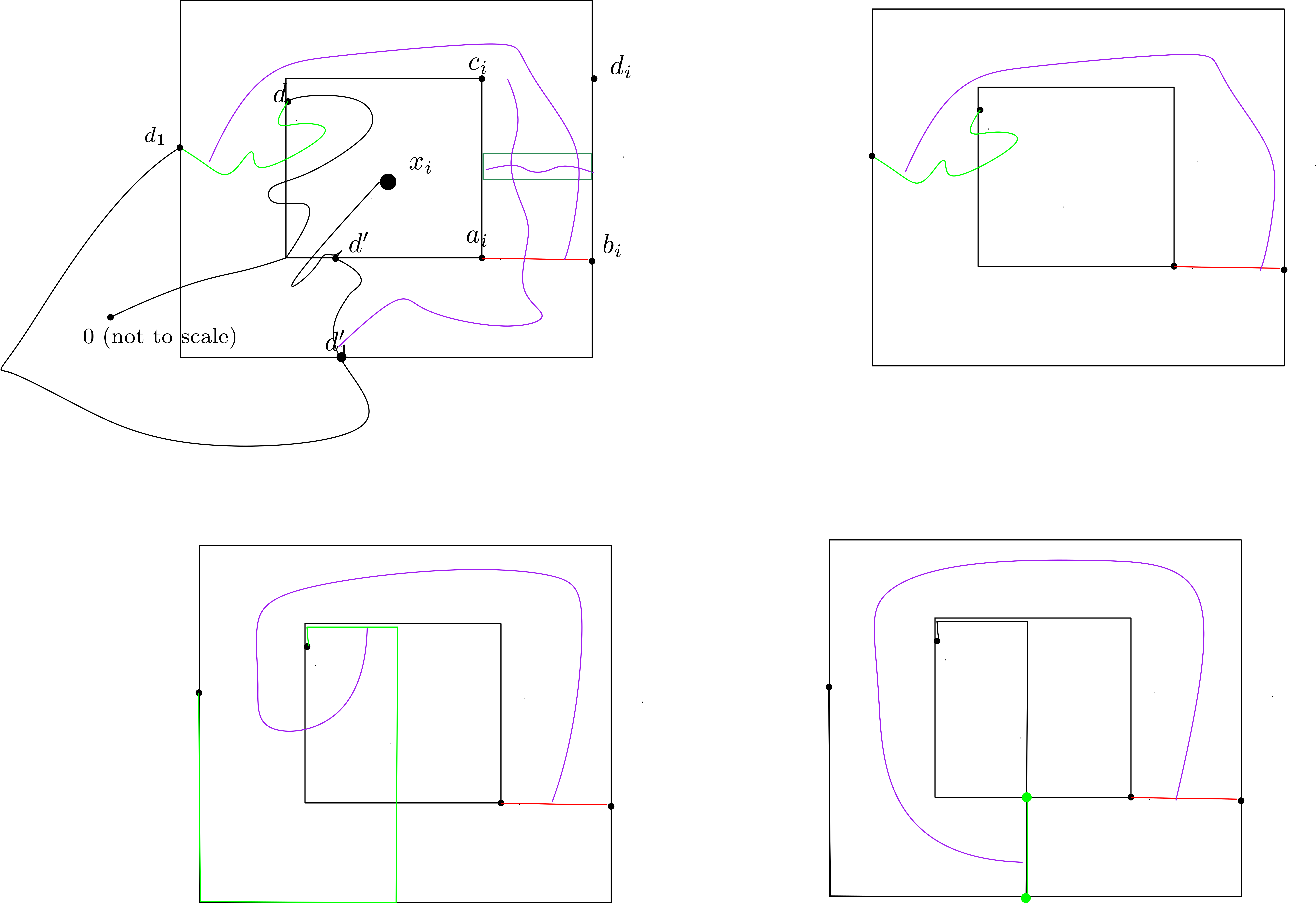
Figure 6: a) The backbone and the paths constructed in the steps in the proof of Lemma 4.5. b) The path $(a_{i}b_{i})\leftrightarrow(dd_{1})$ is (strictly) inside the domain $T_{i,1}$. c) The domain $T_{i,2}$ and the path $(a_{i}b_{i})\leftrightarrow(dd_{1})$. d) The domain $T_{i,3}$ and an example of the path $(a_{i}b_{i})\leftrightarrow(c_{i}d_{i})$

Proof of Lemma 4.6.

We use some ideas from Lemma 3.1 in [40]. Consider a square $B=\Lambda_{\frac{1}{10}}(\frac{3}{2},\frac{1}{20})+x_{i}$ corresponding with the previous lemma such that $L$ passes through $B$. Define the event $\mathcal{S}$ to be $\mathcal{S}_{i}$ where there is also a crossing of each of the four (overlapping) rectangles that make up the annulus $A_{\frac{1}{10},\frac{2}{10}}(\frac{3}{2},\frac{1}{20})$ around $B$ as shown on Figure 7. By RSW for usual rectangles and (FKG) we know that $\phi^{0}_{\Sigma_{i}}(\mathcal{S})\geq c$. By the definition of $\mathcal{S}_{i}$ from Lemma 4.5 $\{x_{i}\leftrightarrow L\}\cap\mathcal{S}=\{x_{i}\leftrightarrow B\}\cap\mathcal{S}$ and so by (FKG) and Lemma 4.5 we get that

$$\phi^{0}_{\Sigma_{i}}\left(x_{i}\leftrightarrow B\mid x_{i}\overset{T_{i}}{\leftrightarrow}A_{i},\mathcal{S}\right)\geq\phi^{0}_{\Sigma_{i}}\left(x_{i}\leftrightarrow L\mid x_{i}\overset{T_{i}}{\leftrightarrow}A_{i},\mathcal{S}\right)\geq c.$$

Now, since

$$\phi^{0}_{\Sigma_{i}}\left(N_{ka^{-\frac{15}{8}},i}\mid x_{i}\leftrightarrow L,x_{i}\overset{T_{i}}{\leftrightarrow}A_{i}\right)\geq\phi^{0}_{\Sigma_{i}}\left(N_{ka^{-\frac{15}{8}},i}\mid x_{i}\leftrightarrow B,x_{i}\overset{T_{i}}{\leftrightarrow}A_{i},\mathcal{S}\right)\phi^{0}_{\Sigma_{i}}\left(x_{i}\leftrightarrow B\mid x_{i}\overset{T_{i}}{\leftrightarrow}A_{i},\mathcal{S}\right)$$

it suffices to prove that

$$\phi^{0}_{\Sigma_{i}}\left(N_{ka^{-\frac{15}{8}},i}\mid x_{i}\leftrightarrow B,x_{i}\overset{T_{i}}{\leftrightarrow}A_{i},\mathcal{S}\right)\geq c.$$

This follows from a second moment estimate. So let $N_{B}=\sum_{z\in B}1_{z\leftrightarrow x_{i}}$. First using the fact that $\mathcal{S}\cap\{x_{i}\leftrightarrow L\}\cap\{z\leftrightarrow\partial\Lambda_{\frac{3}{10}}(x)\}\subset\{x_{i}\leftrightarrow z\}$ and then by (FKG), (MON) and (1-arm) we get

$$\mathbb{E}(N_{B}\mid x_{i}\leftrightarrow B,x_{i}\overset{T_{i}}{\leftrightarrow}A_{i},\mathcal{S}) =\sum_{z\in B}\phi^{0}_{\Sigma_{i}}\left(x_{i}\leftrightarrow z\mid x_{i}\leftrightarrow B,x_{i}\overset{T_{i}}{\leftrightarrow}A_{i},\mathcal{S}\right)$$

$$\geq\sum_{z\in B}\phi^{0}_{\Sigma_{i}}\left(z\leftrightarrow\partial\Lambda_{\frac{3}{10}}(z)\mid x_{i}\leftrightarrow B,x_{i}\overset{T_{i}}{\leftrightarrow}A_{i},\mathcal{S}\right)$$

$$\geq\sum_{z\in B}\phi^{0}_{\Lambda_{\frac{3}{10}}(z)}\left(z\leftrightarrow\partial\Lambda_{\frac{3}{10}}(z)\right)=\frac{1}{100a^{2}}Ca^{\frac{1}{8}}=ca^{-\frac{15}{8}}.$$

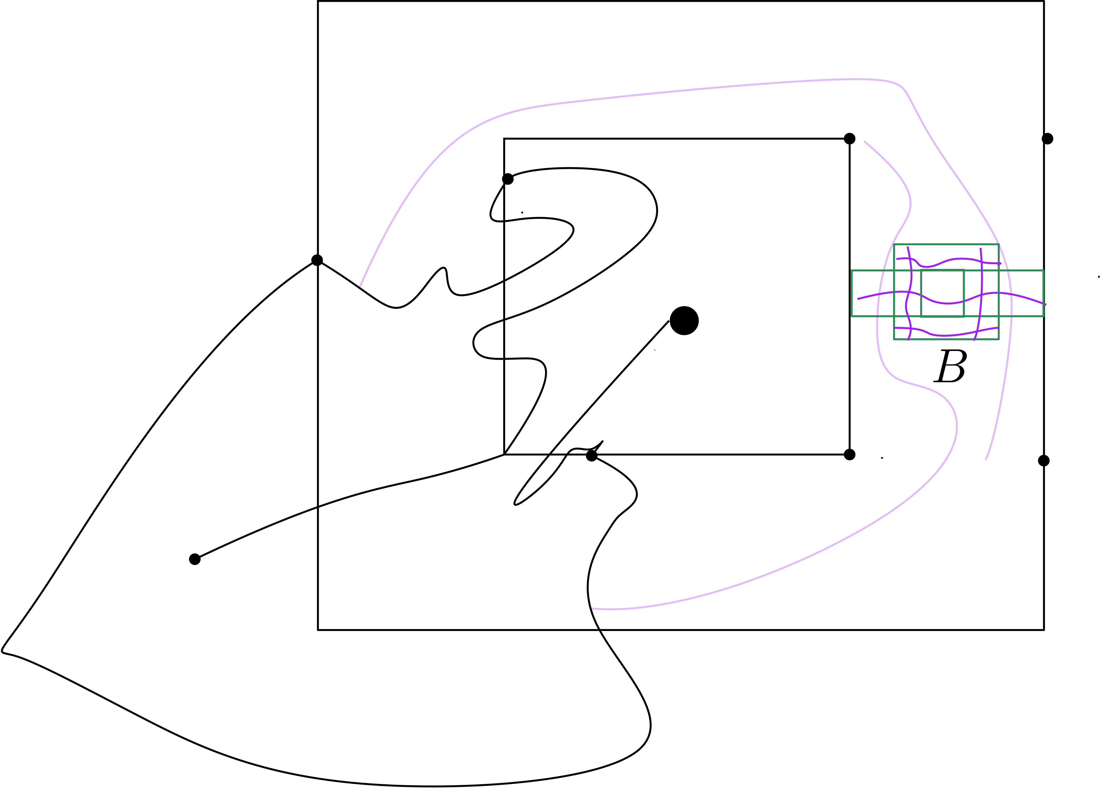
Figure 7: To the right we sketch the situation in Lemma 4.6. We keep the paths that we have seen exist in Lemma 4.5 with constant probability. Then we use RSW to construct some more paths encircling the box $B$ as shown. Later in the proof we split the box $B$ up into dyadic annuli.

Let us then consider the second moment. First we use that $\phi^{0}_{\Sigma_{i}}(x_{i}\leftrightarrow B\mid x_{i}\overset{T_{i}}{\leftrightarrow}A_{i})\geq c$, $\phi^{0}_{\Sigma_{i}}(\mathcal{S})\geq c$ and then we do a dyadic summation for each $z$ partitioning $B$ into annuli $A_{2^{k-1},2^{k}}(z)$ for $k$ such that $-m\leq k\leq 0$ where $m\in\mathbb{N}$ is chosen such that $A_{2^{k-1},2^{k}}(x)=\emptyset$ for $k<-m$.

$$\mathbb{E}(N_{B}^{2}\mid x_{i}\leftrightarrow B,x_{i}\overset{T_{i}}{\leftrightarrow}A_{i},\mathcal{S})=\sum_{z,y\in B}\phi^{0}_{\Sigma_{i}}\left(x_{i}\leftrightarrow z,x_{i}\leftrightarrow y\mid x_{i}\leftrightarrow B,x_{i}\overset{T_{i}}{\leftrightarrow}A_{i},\mathcal{S}\right)$$

$$\leq\frac{c}{\phi^{0}_{\Sigma_{i}}(x_{i}\overset{T_{i}}{\leftrightarrow}A_{i})}\sum_{z,y\in B}\phi^{0}_{\Sigma_{i}}\left(x_{i}\leftrightarrow z,x_{i}\leftrightarrow y,x_{i}\overset{T_{i}}{\leftrightarrow}A_{i}\right)$$

$$\leq\frac{c}{\phi^{0}_{\Sigma_{i}}(x_{i}\overset{T_{i}}{\leftrightarrow}A_{i})}\sum_{z\in B}\sum_{k=-m}^{0}\sum_{y\in A_{2^{k-1},2^{k}}(z)}\phi^{0}_{\Sigma_{i}}\left(z\leftrightarrow\partial\Lambda_{2^{k-2}}(z),y\leftrightarrow\partial\Lambda_{2^{k-2}}(y),x_{i}\leftrightarrow\partial\Lambda_{\frac{1}{20},\frac{1}{20}}(x_{i})\right)$$

$$\leq\frac{c\phi^{0}_{\Sigma_{i}}(x_{i}\leftrightarrow\partial\Lambda_{\frac{1}{20},\frac{1}{20}}(x_{i}))}{\phi^{0}_{\Sigma_{i}}(x_{i}\overset{T_{i}}{\leftrightarrow}A_{i})}\sum_{z\in B}\sum_{k=-m}^{0}\sum_{y\in A_{2^{k-1},2^{k}}(z)}\phi^{0}_{\Sigma_{i}}\left(z\leftrightarrow\partial\Lambda_{2^{k-2}}(z)\right)\phi^{0}_{\Sigma_{i}}\left(y\leftrightarrow\partial\Lambda_{2^{k-2}}(y)\right)$$

$$\leq\sum_{z\in B}\sum_{k=-m}^{0}c_{1}\left(\frac{2^{k}}{a}\right)^{2}\left(\frac{a}{2^{k-2}}\right)^{\frac{2}{8}}=c_{2}a^{-2}a^{-2}a^{\frac{1}{4}}\sum_{k=-m}^{0}2^{2k-\frac{k}{4}}=c_{3}a^{-\frac{15}{4}}$$

where we also used (1-arm) several times and that (Mixing) holds at all scales smaller than our fixed macroscopic scale. The conclusion follows from the Paley-Zygmund inequality

$$\phi^{0}_{\Sigma_{i}}\left(N_{ka^{-\frac{15}{8}},i}\mid x_{i}\leftrightarrow B,x_{i}\overset{T_{i}}{\leftrightarrow}A_{i},\mathcal{S}\right)\geq ca^{\frac{15}{4}-\frac{15}{4}}=c.$$

∎

Finally, let us prove Proposition 3.3.

Proof of Proposition 3.3.

By Proposition 4.1 it suffices to prove $\phi^{0}_{\Sigma_{i}}\left(x_{i}\overset{T_{i}}{\leftrightarrow}\mathrm{g}\mid x_{i}\leftrightarrow A_{i}\right)\geq c$ and the similar inequality for $\tilde{T}$ and $\tilde{x}$ which will follow in the same way. First, notice that by Lemma 4.5 and Lemma 4.6

$$\phi^{0}_{\Sigma_{i}}\left(N_{ka^{-\frac{15}{8}},i}\mid x_{i}\leftrightarrow A_{i}\right)\geq\phi^{0}_{\Sigma_{i}}\left(N_{ka^{-\frac{15}{8}},i}\mid x_{i}\leftrightarrow L,x_{i}\leftrightarrow A_{i}\right)\phi^{0}_{\Sigma_{i}}\left(x_{i}\leftrightarrow L\mid x_{i}\leftrightarrow A_{i}\right)\geq c\cdot c$$

Now, we can make the following observation using Lemma 2.2 to find

$$\phi^{0}_{\Sigma_{i}}(x_{i}\overset{T_{i}}{\leftrightarrow}\mathrm{g}\mid x_{i}\leftrightarrow A_{i}) \geq\phi^{0}_{\Sigma_{i}}\left(N_{ka^{-\frac{15}{8}},i},x_{i}\overset{T_{i}}{\leftrightarrow}\mathrm{g}\mid x_{i}\leftrightarrow A_{i}\right)$$

$$=\phi^{0}_{\Sigma_{i}}\left(x_{i}\overset{T_{i}}{\leftrightarrow}\mathrm{g}\mid N_{ka^{-\frac{15}{8}},i},x_{i}\leftrightarrow A_{i}\right)\phi^{0}_{\Sigma_{i}}\left(N_{ka^{-\frac{15}{8}},i}\mid x_{i}\leftrightarrow A_{i}\right)$$

$$\geq\tanh\left(ka^{-\frac{15}{8}}ha^{\frac{15}{8}}\right)c\geq c(k,h).\qed$$

References

- [1] Federico Camia, Jianping Jiang, and Charles Newman. Exponential Decay for the Near‐Critical Scaling Limit of the Planar Ising Model. Communications on Pure and Applied Mathematics, 07 2020.
- [2] Michael Aizenman, Hugo Duminil-Copin, Vincent Tassion, and Simone Warzel. Emergent planarity in two-dimensional ising models with finite-range interactions. Inventiones mathematicae, 216:661–743, 2018.
- [3] Hugo Duminil-Copin and Ioan Manolescu. Planar random-cluster model: scaling relations, 2020. arXiv:2011.15090.
- [4] E. Ising. Beitrag zur Theorie des Ferromagnetismus. Z. Phys.31 253-258, 1925.
- [5] W. Lenz. Beitrag zum Verständnis der magnetischen Erscheinungen in festen Körpern. Physik Zeitschr. 21 613-615, 1920.
- [6] G. Grimmett. The random-cluster model. volume 333 of Grundlehren der Mathematischen Wissenschaften [Fundamental Principles of Mathematical Sciences]., 2006.
- [7] H.Duminil-Copin. Lectures on the Ising and Potts models on the hypercubic lattice. PIMS-CRM Summer School in Probability, 2019.
- [8] R. Periels. On Ising’s model on ferromagentism. Proc. Cambrigde Phil. Soc. 32 477-481, 1936.
- [9] L. Onsager. Crystal statistics. I. A two-dimensional model with an order-disorder transition. Phys. Rev. 65 117-149, 1944.
- [10] Stanislav Smirnov. Conformal invariance in random cluster models. I. Holmorphic fermions in the Ising model. Annals of Mathematics, 172:1435–1467, 09 2010.
- [11] Dmitry Chelkak and Stanislav Smirnov. Universality in the 2D Ising model and conformal invariance of fermionic observables. Inventiones mathematicae, 189:515–580, 2009.
- [12] Hugo Duminil-Copin and S.Smirnov. Probability and statistical physics in two and more dimensions. Clay Math. Proc., 15:213–276., 2012.
- [13] Federico Camia, Christophe Garban, and Charles Newman. Planar Ising magnetization field II. Properties of the critical and near-critical scaling limits. Annales de l’Institut Henri Poincaré, Probabilités et Statistiques, 52, 07 2013.
- [14] Federico Camia, René Conijn, and Demeter Kiss. Conformal Measure Ensembles for Percolation and the FK–Ising Model, pages 44–89. 01 2019.
- [15] Federico Camia, Jianping Jiang, and Charles M. Newman. Conformal Measure Ensembles and Planar Ising Magnetization: A Review, 2020. arXiv:2009.08129.
- [16] Federico Camia, Jianping Jiang, and Charles Newman. New FK-Ising coupling applied to near-critical planar models. Stochastic Processes and their Applications, 09 2017.
- [17] A. B. Zamolodchikov. Integrals of motion and -matrix of the (scaled) Ising model with magnetic field. International Journal of Modern Physics A, 04, 04 2012.
- [18] G. Mussardo. Statistical Field Theory: An Introduction to Exactly Solved Models in Statistical Physics. 03 2020.
- [19] David Borthwick and Skip Garibaldi. Did a 1-dimensional magnet detect a 248-dimensional Lie Algebra? Notices of the AMS, 2011.
- [20] R. Coldea et al. Quantum Criticality in an Ising chain: Experimental Evidence for Emergent symmetry . Science, 327, 177-180, 2010.
- [21] Kirill Amelin, Johannes Engelmayer, Johan Viirok, Urmas Nagel, Toomas Rõ om, Thomas Lorenz, and Zhe Wang. Experimental observation of quantum many-body excitations of symmetry in the Ising chain ferromagnet . Phys. Rev. B, 102:104431, Sep 2020.
- [22] Zhao Zhang, Kirill Amelin, Xiao Wang, Haiyuan Zou, Jiahao Yang, Urmas Nagel, Toomas Rõ om, Tusharkanti Dey, Agustinus Agung Nugroho, Thomas Lorenz, Jianda Wu, and Zhe Wang. Observation of particles in an ising chain antiferromagnet. Phys. Rev. B, 101:220411, Jun 2020.
- [23] M. Hasenbusch M. Caselle. Critical amplitudes and mass spectrum of the 2d Ising model in a magnetic field . Nuclear Physics B ,579(3), 667-703, 2000.
- [24] O.Penrose and J.L. Lebowitz. Analytic and Clustering Properties of Thermodynamic Functions and Distribution Functions for Classical Lattice Systems and Continuum Systems . Communications in Mathematical Physics, 11:99–124, 1968.
- [25] Jürg Fröhlich and Pierre-François Rodriguez. Some Applications of the Lee-Yang Theorem. Journal of Mathematical Physics, 53, 05 2012.
- [26] Federico Camia, Jianping Jiang, and Charles Newman. A Gaussian Process Related to the Mass Spectrum of the Near-Critical Ising Model. Journal of Statistical Physics, 179, 05 2020.
- [27] Sacha Friedli and Yvan Velenik. Statistical Mechanics of Lattice Systems: a Concrete Mathematical Introduction. 11 2017.
- [28] Aran Raoufi. Translation-invariant Gibbs states of the Ising model: general setting. The Annals of Probability, 48(2):760–777, 2020.
- [29] Michael Aizenman. Geometric Analysis of Fields and Ising Models (Parts 1 & 2). Commun. Math. Phys., 86:1, 1982.
- [30] Michael Aizenman and Hugo Duminil-Copin. Marginal triviality of the scaling limits of critical 4D Ising and models. Annals of Mathematics, 194(1):163–235, 2021.
- [31] Michael Aizenman, David J. Barsky, and Roberto Fernández. The phase transition in a general class of Ising-type models is sharp. Journal of Statistical Physics, 47:343–374, 1987.
- [32] Michael Aizenman, Hugo Duminil-Copin, and Vladas Sidoravicius. Random Currents and Continuity of Ising Model’s Spontaneous Magnetization. Communications in Mathematical Physics, 334, 11 2013.
- [33] A. Sakai. Lace expansion for the ising model. Communications in Mathematical Physics, 272:283–344, 2005.
- [34] S. Shlosman. Signs of the ising model ursell functions. Communications in Mathematical Physics, 102:679–686, 1986.
- [35] H. Duminil-Copin. Random current expansion of the Ising model. Proceedings of the 7th European Congress of Mathematicians in Berlin, 2016.
- [36] Robert B. Griffiths, Charles Angas Hurst, and Seymour Sherman. Concavity of Magnetization of an Ising Ferromagnet in a Positive External Field. Journal of Mathematical Physics 11, 790, 1970.
- [37] Hugo Duminil-Copin, Clément Hongler, and Pierre Nolin. Connection Probabilities and RSW-Type Bounds for the Two-Dimensional FK Ising Model. Communications on Pure and Applied Mathematics, 64, 09 2011.
- [38] Dmitry Chelkak, Hugo Duminil-Copin, and Clément Hongler. Crossing Probabilities in Topological Rectangles for the Critical Planar FK-Ising model. Electronic Journal of Probability, 21, 12 2013.
- [39] Dmitry Chelkak. Robust Discrete Complex Analysis: A Toolbox. The Annals of Probability, 44, 12 2012.
- [40] Federico Camia, Christophe Garban, and Charles Newman. Planar Ising magnetization field I. Uniqueness of the critical scaling limit. The Annals of Probability, 43, 05 2012.