Simultaneous predictive bands for functional time series using minimum entropy sets

Abstract

Functional Time Series (FTS) are sequences of dependent random elements taking values on some functional space. Most of the research on this domain focuses on producing a predictor able to forecast the next function, having observed a part of the sequence. For this, the Autoregressive Hilbertian process is a suitable framework. Here, we address the problem of constructing simultaneous predictive confidence bands for a stationary FTS. The method is based on an entropy measure for stochastic processes. To construct predictive bands, we use a Reproducing Kernel Hilbert Spaces (RKHS) to represent the functions and a functional bootstrap procedure that allows us to estimate the prediction law and a Reproducing Kernel Hilbert Spaces (RKHS) to represent the functions, considering then the basis associated to the reproducing kernel. We then classify the points on the projected space according to those that belong to the minimum entropy set (MES) and those that do not. We map the minimum entropy set back to the functional space and construct a band using the regularity property of the RKHS. The proposed methodology is illustrated through artificial and real data sets.

1 Introduction

While Functional Data Analysis Ramsay, (2006) deals with independent and identical distributed realizations of functional data, the term Functional Time Series (FTS) refers to dependent series of random elements lying in some functional space. Alongside the academic research interest awoken by such an elegant framework, FTS have important practical usefulness. In some cases, they allow one to consider an alternative modelling scheme to classical time series, thanks to their ability to intrinsically deal with non-stationary patterns such as seasonality. Moreover, they can be of great help if one has a heterogeneous sampling scheme where records are observed at unequally spaced time points.

A simple yet powerful device to construct a FTS is proposed by Bosq, (2000). The idea is to take slices of an underlying continuous stochastic process, say $\xi=\{\xi(t);t\in\mathbb{R}\}$, using a window of fixed size $\delta>0$. We then consider the FTS $Z$ such that $Z_{k}(t)=\xi((k-1)\delta+t)$ with $k\in\mathbb{Z}$ and $t\in(0,\delta)$. In many real data applications, this scheme is reasonable: an underlying phenomenon of continuous nature exists even if data are recorded at some sampling rate. Examples of this can be found, for example, in electrical device monitors (Bonnevay et al., , 2019), energy demand (Antoniadis et al., , 2016), air pollution (Paparoditis and Shang, , 2020) and geology (Hörmann et al., , 2010). Note that the device is particularly fruitful if the quantity $\delta$ is tailored to some seasonal component of the series $\xi$. In such cases, the series $Z$ naturally incorporates the non-stationary pattern induced by the seasonality. Other kinds of FTS involve more general situations, as for instance sequences of functions that do not verify continuity constraints between consecutive functions (see Aue et al., (2015)).

One important task related to FTS is forecasting. That is, after having observed $n$ realizations of the process $Z$, say $Z_{1},\ldots,Z_{n}$, the aim is to predict the next whole function $Z_{n+1}(t),t\in(0,\delta)$. Autoregressive Hilbertian processes (ARH) are the natural extension of univariate autoregressive processes to the functional data framework where Hilbert spaces are considered. The term Functional Autoregressive is sometimes also used to name the same process, while this can produce confusion with univariate autoregressive non-linear processes. In short, they consist of linking two consecutive functions of a stationary FTS through a linear operator plus a functional noise. Since the functions are usually supposed to take values on some Hilbert space, the processes are also named Autoregressive Hilbertian (ARH). An excellent review of these processes can be found in Alvarez-Liébana, (2017). Several works address the problem of predicting the function $Z_{n+1}(t)$ using variants of ARH (Aue et al., , 2015; Nagbe et al., , 2018; Wang et al., , 2020); in a more general framework such as a non-linear version of FTS (Antoniadis et al., , 2006), or using Factor Models (Tavakoli et al., , 2023).

While point prediction gives helpful information about the future evolution of FTS, uncertainty quantification is often needed to produce valid inferences. Estimating the predictive law has received much less attention in the FTS literature. In general, bootstrap methods are used to produce pseudo-predictions. Some form of central region is then taken to be the predictive band. For instance, Hyndman and Shang, (2009) describe the FTS as a set of univariate time series associated to projected components. Then, using classical time series tools, they produce individual predictions and pseudo-predictions based on a residual bootstrap. The univariate pseudo-predictions are mapped back to the functional space to obtain functional pseudo-predictions. With this, the band is constructed on a point-by-point basis taking the quantiles at some coverage level. Antoniadis et al., (2012) use a non-linear version of FTS where the predictor is a weighted mean of functions with weights increasing with the similarity between the last observed function and every function in the dataset. The set of weights is the key element of the bootstrap procedure since the more a function is similar with the current one, the more likely the chances of its next function are to be sampled. The band is constructed using heuristics coming from econometric literature. In Paparoditis and Shang, (2020) the authors propose a model-free bootstrap procedure based on the prediction generated by a vector autoregressive model (VAR) applied to the coefficients of the Karhunen-Loève expansion of the FTS. Then simultaneous and pointwise intervals for the prediction are constructed using the bootstrap studentized prediction error.

In this paper we address the problem of constructing a confidence band for the prediction of the FTS. The aim is to construct a region $\mathcal{B}^{1-\alpha}_{n+1}$ which covers the function $Z_{n+1}(t)$, that is $P(Z_{n+1}(t)\in\mathcal{B}^{1-\alpha}_{n+1})\geq 1-\alpha$ for a fixed risk level $\alpha\in(0,1)$. The probability measure is found using the information available at the moment $n$. Note that this prediction band requires simultaneous coverage of the whole curve $Z_{n+1}(t)$, which, in general, is a difficult requirement (see Degras, (2017) for a discussion in the functional data context). Since it is usual to represent functions by the projection coefficients over a basis, some works have explored the option of constructing a confidence region on the coefficients space (Antoniadis et al., , 2006, 2012). However, obtaining simultaneous confidence bands sometimes requires additional regularity assumptions on the functional spaces Genovese and Wasserman, (2005).

Probability densities play an important role in the construction of predictive intervals. However, for functional data the concept of density cannot be well defined in the functional space. In this sense, as the usual workflow is designed to deal with the projected coefficients of the functions in some basis Delaigle et al., (2010) propose that we consider the probability density in such multivariate space. The construction of probability regions in the projected space can be sorted out by means of a metric e.g., a distance that induces an order in that space. This metric can be a depth function, (Fraiman and Muniz, (2001); López-Pintado and Romo, (2009); Cuevas et al., (2007), among others); a distance (Galeano et al., (2015); Martos et al., (2014); Cardot et al., (2013) and the references therein); or an information theory tool such as entropy (Martos et al., (2018)). These three concepts are linked in the sense that they induce an order in a functional data set and allow the construction of $(1-\alpha)$-central regions in the original space where the functions inhabit. Ideally, the main condition that these $(1-\alpha)$-central regions should satisfy is that they concentrate a high amount (at least $1-\alpha\text{, with }\alpha\in[0,1]$) of probability inside. In multivariate spaces, these $(1-\alpha)$-central regions are known in the literature as high density regions (HDR), see Hyndman, (1996).

In this paper we propose to use Minimum Entropy Sets (MES) as a way to estimate the HDR of the predictive law of the projection coefficients to then construct prediction bands. Our procedure can be used on top of any FTS forecasting approach, providing a predictor and a bootstrap method. Additional regularity of the functional space may be required to map the MES back on to the functional space. Our choice is to work on the special case of Hilbert spaces given by reproducing kernels (RKHS) that ensures the continuity of the pointwise evaluation functional.

We illustrate our procedure in Figure 1. Departing from a functional time series $Z$, we obtain the h-step ahead prediction using, for example, an ARH(1) functional model. Using the residual based functional bootstrap procedure presented in Section 3.2 we obtain the sample of predictive pseudo-replicates. These are represented as grey curves in the background of the leftmost graphic. The functions are projected into an appropriate space $\mathcal{H}_{k}\subset\mathcal{H}$ (defined in Section 2.1) and now work on the coefficients of that projection (rightmost graphic). Then, we compute the MES of this new space, for different values of confidence $1-\alpha$ (in the example we use $\alpha=\{0.05,0.1,0.2\}$). The final step involves the back-mapping of these sets to the functional space. For this, we identify each point covered by the MES on the right with its associated curve on the left. Finally, the predictive confidence band is the convex-hull of the curves associated to the MES.

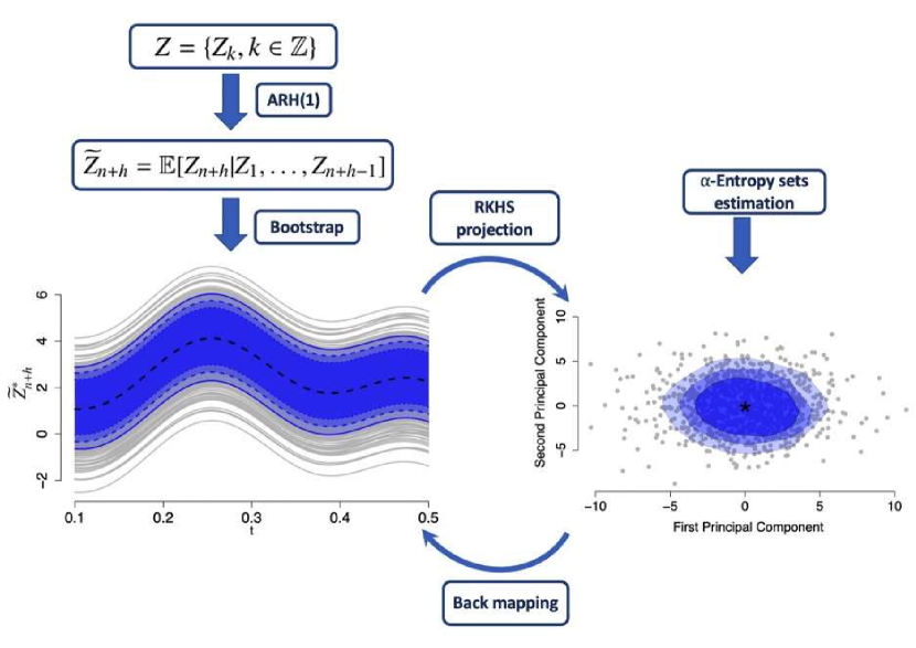
Figure 1: Band construction procedure.

The paper is organized as follows: in Section 2 we present the RKHS framework needed for representing the ARH processes in such spaces, as well as considerations about the simulation, estimation and prediction procedures. We focus on predictive inference in Section 3, defining Minimum Entropy Sets, a bootstrap procedure compatible with FTS and the predictive confidence bands methodology. Section 4 describes the experimental design using Monte Carlo simulation to show the good covering results of our proposal and a real data application. We conclude the paper with Section 5.

2 The autoregressive Hilbertian model: ARH

In this section we introduce notation and recall well-known facts about representing a function with Reproducing Kernel Hilbert Spaces (RKHS) and autoregressive Hilbert (ARH) processes. All the random elements below are defined in the same probability space $(\Omega,\mathcal{F},P)$.

2.1 Representing functional data using RKHS

In general, we cannot observe the full trajectories of functional variable realisations. Since it is also the case for FTS, our input data is the set of discrete and noisy trajectories that constitutes realisations of the functional variable, also known in the literature as raw functional data (Hsing and Eubank, , 2015). In what follows, we set the functional space $\mathcal{H}\subset C[T]$ the space of (classes of) real continuous functions over the compact T -. In our case we set $T=[0,\delta]$, with $\delta=1$ without loss of generality. In that sense, raw functional data consist of the collection of the functions recorded over a grid of $m$ discretized points, say $t_{1},\dots,t_{m}$ (usually equally spaced). The analysis departs from a collection of discrete functions, hereafter curves: $\{z_{j}(t_{i})\}_{i=1}^{m}\text{ for }j=1,\dots,n$.

As is usual in the functional data literature, in order to estimate the underlying functional object that generated each realisation $z_{j}$ we need to choose a system of orthonormal basis functions. Following the approach in Muñoz and González, (2010); Berlinet and Thomas-Agnan, (2011), we propose to chose $\mathcal{H}=\mathcal{H}_{K}$ as a RKHS, such that the family of basis functions $\Phi=\{\phi_{1},\dots,\phi_{d}\}$ generates the functional subspace $\mathcal{H}_{K}$ through its linear span. These basis functions are linked to the positive-semidefinite kernel function $K=K(s,t)$ associated to $\mathcal{H}_{K}$. Any realisation $z(t)$ can be approximated by the following functional estimator

$$\tilde{z}(t):=\operatorname{arg}\min_{f\in\mathcal{H}}\sum^{m}_{i=1}L(z(t_{i}),f(t_{i}))+\gamma\|f\|_{\mathcal{H}}^{2},$$ (1)

where $\gamma>0$ is a regularization parameter, $\|f\|_{\mathcal{H}}$ is the norm of the function $f$ in $\mathcal{H}$ and $L(w,z)=(w-z)^{2}$ is a loss function. By the Representer Theorem (Cucker and Smale, , 2002, Theorem 5.2, p. 91) the solution of the problem stated in Eq. (1) exists, is unique, and admits the following representation

$$\tilde{z}(t)=\sum_{i=1}^{m}a_{i}K(t_{i},t)=\textbf{a}^{T}\mathbf{K}_{t},$$ (2)

where $\mathbf{K}_{t}=\{K(t_{1},t),\dots,K(t_{m},t)\}$ is the vector of kernel evaluations and the linear combination coefficients $\textbf{a}=(a_{1},\dots,a_{m})\in\mathbb{R}^{m}$ are obtained as the solution to the linear system $(\gamma\mathbf{I}_{m}+\textbf{K})\textbf{a}=\mathbf{z}$, for $\mathbf{z}=(z(t_{1}),\dots,z(t_{m}))^{T}$, $\mathbf{I}_{m}$ an $m\times m$ identity matrix, and K the Gram matrix with the kernel function evaluations over the grid $t_{1},\dots,t_{m}$. Now, we use the Mercer decomposition theorem (J Mercer, , 1909) to obtain the basis. Indeed, since K is a positive-definite and symmetric kernel function with associated integral operator $I_{K}(z)=\int_{T}K(\cdot,t)z(t)dt$, it admits a spectral decomposition into a sequence $(\lambda_{i},\phi_{i})_{i\geq 1}$ of eigenvalue-eigenfunction pairs. Note that in this scheme, one chooses the kernel K, which determines the basis, which is the converse of usual FDA practice. Then, each estimated functional datum $\tilde{z}(t)$ in the sample can be expressed as follows

$$\tilde{z}(t)=\sum_{i=1}^{m}c_{i}\phi_{i}(t),$$ (3)

where $c_{i}$ are the projection coefficients of $\tilde{z}(t)$ onto the space generated by the eigenfunctions $\phi_{i}$. Nevertheless, the expression in Eq. (3) is an unhelpful representation when the sequence of eigenpairs $(\lambda_{i},\phi_{i})_{i\geq 1}$ is unknown. With the sample data at hand, $c_{i}$ can be estimated by:

$$\hat{c}_{i}=\displaystyle\frac{l_{i}}{\sqrt{m}}(\textbf{a}^{T}\mathbf{v}_{i}),$$ (4)

where $(l_{i},\mathbf{v}_{i})$ are the $i^{th}$ eigenvalue (in decreasing order) and eigenvector of K. It is possible to approximate the development in Eq. (3) by truncating the sum by the first few terms. Therefore, we represent each function $z(t)$ with a finite representation in $\mathbb{R}^{d}$ given by $\hat{\boldsymbol{c}}=\{\hat{c}_{1},\dots,\hat{c}_{d}\}$, where $d\leq\text{rank}(\textbf{K}$). Then, the function bases are truncated and the projection coefficients approximated via equation (4). The dimension $d$ is simply a truncation order, not something intrinsic to the kernel $K$ or space $\mathcal{H}$.

2.2 Autoregressive Hilbert process

Following the previous notation, the sequence $Z=\{Z_{k},k\in\mathbb{Z}\}$ of random functions on $\mathcal{H}$ follows an ARH(1) if,

$$Z_{k}=\mu+\Psi(Z_{k-1}-\mu)+\epsilon_{k},$$ (5)

where $\mu$ is the mean function, $\Psi$ is a linear bounded (continuous) operator on $\mathcal{H}\mapsto\mathcal{H}$ and $\epsilon=\{\epsilon_{k},k\in\mathbb{Z}\}$ a strong white noise in $\mathcal{H}$ such that $\mathbb{E}\|\epsilon_{k}\|<\infty$ and $E[Z_{0}]=\mu$, $E\|Z_{0}\|^{2}<\infty$. Under mild conditions, the expression defined in Eq. (5) defines a strictly stationary stochastic process in $\mathcal{H}$. Given $Z_{1},\ldots,Z_{n}$, the best predictor of the function $Z_{n+1}$ in the mean-square-error sense is given by

$$\widetilde{Z}_{n+1}=\mathbb{E}[Z_{n+1}|Z_{1},\ldots,Z_{n}],$$ (6)

which results for the ARH process in $\widetilde{Z}_{n+1}=\mu+\Psi(Z_{n}-\mu)$. This predictor is not statistical in nature because it depends on parameters of the unknown probability law. Therefore, one needs to estimate $\mu$ and $\Psi$ to get a statistical predictor. A simple way is to use the empirical counterpart of the population mean to estimate the mean function. The estimation of $\Psi$ is more cumbersome because it involves unbounded operators. For this, the cross-covariance operator of lag $r$ is defined as

$$\Gamma_{r}=\mathbb{E}[(Z_{0}-\mu)\otimes(Z_{r}-\mu)],$$ (7)

which under mild conditions is a trace-class operator. To estimate the operator $\Psi$ we use the covariance operator ($\Gamma_{0}$) and the cross-covariance operator ($\Gamma_{1}$), related by a Yule-Walker like expression (see Bosq, (2000)),

$$\Gamma_{0}\Psi=\Gamma_{1}.$$ (8)

If $\mathcal{H}$ is of finite dimension, then one can just plug in the empirical counterparts of $\Gamma_{0}$ and $\Gamma_{1}$ and solve to obtain $\Psi$. However, in the general case the unboundedness of the inverse of $\Gamma_{0}$ implies that the expression in Eq. 8 is an ill-posed problem, see Mas and Pumo, (2011) for a detailed discussion. Fortunately, the problem has more impact for the development of theoretical results. The empirical equivalents of the operators are matrices and one relies on regularized versions of the inverse of the covariance matrix to obtain the estimation of $\Psi$. A second important property of ARH processes is worth mentioning since it is used for simulation. Indeed, if $Z$ follows an ARH(1), then

$$\Gamma_{\epsilon}=\Gamma_{0}-\Psi\Gamma_{0}\Psi^{T},$$ (9)

where $\Gamma_{\epsilon}$ is the covariance operator of $\epsilon$ (Bosq, , 2000, Chap 3.). This means that only two of the three operators can be chosen freely for the simulation of ARH trajectories. Moreover, since $\Gamma_{\epsilon}$ needs to be positive-definite, not every couple of $\Psi$ and $\Gamma_{0}$ will produce a compatible innovation process $\epsilon$.

Estimation and prediction

In practice, only finite measurements on each function are used to estimate the parameter. Given the finite, truncated representation of each curve in Eq. 3 and the estimated coefficients, $\hat{c}_{i}$, the mean function can be estimated by

$$\hat{\mu}(t)=\sum_{i=1}^{d}\bar{\hat{c}}_{i}\phi_{i}(t),\qquad\text{with}\;\;\bar{\hat{c}}_{i}=\frac{1}{n}\sum_{k=1}^{n}\hat{c}_{k,i}.$$ (10)

As it is usual in FDA the operation concerns the projection coefficients, which are then expanded on the basis constructed using a kernel function. Similarly, the corresponding covariance $\hat{\Gamma}_{0}$ and cross-covariance $\hat{\Gamma}_{1}$ estimators of the operators $\Gamma_{0}$ and $\Gamma_{1}$ are

$$\widehat{\Gamma}_{r}=\frac{1}{n-r}\sum_{k=1}^{n-r}\sum_{i^{\prime}=1}^{d}\sum_{i=1}^{d}\hat{d}_{k,i}\hat{d}_{k,i^{\prime}+r}\phi_{i}\otimes\phi_{i^{\prime}},\qquad r=0,1,$$ (11)

where $\hat{d}_{k,i}=\hat{c}_{k,i}-\bar{\hat{c}}_{i}$. Note that the coefficients can be arranged into two squared $d\times d$ matrices, say $\mathbf{\hat{C}_{0}}$ and $\mathbf{\hat{C}_{1}}$,

$$(\mathbf{\widehat{C}_{r}})_{i,i^{\prime}}=\frac{1}{n-r}\sum_{k=1}^{n-r}\hat{d}_{k,i}\hat{d}_{k,i^{\prime}+r},\qquad r=0,1.$$ (12)

At this point, one can estimate the projection coefficients of $\Psi$ on the double basis induced by the kernel. For this, we solve the equivalent of Eq. (8) to obtain $\mathbf{\widehat{P}}=\mathbf{\widehat{C}_{0}^{-1}}\mathbf{\widehat{C}_{1}}$. Note that the truncation introduced in Section 2.1 sized down these matrices to $d<m$. Besides the trivial reduction on the computation times of these matrices, the truncation induces a regularization effect needed to better approximate the operator $\Psi$ (see Bosq, (2000)). Finally, $\Psi$ is estimated by:

$$\widehat{\Psi}=\sum_{i^{\prime}=1}^{d}\sum_{i=1}^{d}\hat{p}_{i,i^{\prime}}\phi_{i}\otimes\phi_{i^{\prime}},$$ (13)

where $\hat{p}_{i,i^{\prime}}=(\mathbf{\widehat{P}})_{i,i^{\prime}}$. The one-step-ahead prediction $\widehat{Z}_{n+1|n}$ is obtained by applying $\widehat{\Psi}$ to the last observed function.

Simulation

We adopt a straightforward approach to simulate an ARH as in Didericksen et al., (2012). Following equation (5), the idea is to sequentially produce a FTS by applying the iteration after an arbitrary initialisation. By the ergodicity, one can expect that the obtained FTS follows the given ARH after a reasonable burn-in period. This scheme is particularly fruitful to test different variants for $\mu$ and specifically for $\Psi$ (for instance symmetric and asymmetric operators). Moreover, one can choose different noise processes, which is important in the assessment of prediction bands. Importantly to notice, the explicit choices of the noise process (and its covariance operator $\Gamma_{\epsilon}$) and the autoregression operator $\Psi$ determine the variance operator $\Gamma_{0}$ of the FTS $X$.

3 Making predictive inference with the ARH-RKHS model

Prediction is one of the main objectives in time series analysis. In terms of uncertainty, prediction intervals bring more information about the future values of a random variable than point forecasts. In that sense, prediction intervals entail a set of values that the realisation of the future random variable could take, conditional on past information and given a certain probability. In the functional time series context, given the functional nature of the observations, the predictive confidence intervals take the form of predictive confidence bands (PCB), which implies the definition of a bounded region in the original space, $\mathcal{H}$, which the functions inhabit, such that if we randomly take one realisation of the sample of functional time series, it will be fully enclosed by the band with a given probability.

We define the lower and upper functional statistics, $L_{n+1|n}(t)$ and $U_{n+1|n}(t)$ both in $\mathcal{H}$ such that the region comprised by $\{[L_{n+1|n}(t),U_{n+1|n}(t)]:t\in T\}$ fully contains the conditional expectation $\widetilde{Z}_{n+1|n}$ (see Eq. (6)) with a probability of $1-\alpha$.

Definition 1.

Let $L_{n+1|n}(t)$ and $U_{n+1|n}(t)$ be two elements of $\mathcal{H}$. We define a predictive confidence band as the set $\mathcal{B}^{1-\alpha}_{n+1|n}=\{(t,z)\in R^{2}:L_{n+1|n}(t)\leq z\leq U_{n+1|n}(t),t\in T\}$, such that

$$P\big{(}\widetilde{Z}_{n+1|n}\in\mathcal{B}^{1-\alpha}_{n+1|n},\forall t\in T\big{)}\geq 1-\alpha.$$ (14)

Following Degras, (2017), there are at least two options to conduct predictive inference in the functional context: i) pointwisely or ii) simultaneously. Under the pointwise estimation of $\mathcal{B}^{1-\alpha}$ the condition stated in Eq. 14 is satisfied for each $t\in T$, independently. Let say the prediction is sampled at $m$ points in the domain $T$, then the pointwise confidence band, $\mathcal{\widehat{B}}^{1-\alpha,p}_{n+1|n}$ is constructed by the concatenation of $m$ prediction intervals $[L_{n+1|n}^{p}(t_{i}),U_{n+1|n}^{p}(t_{i})]$ for each $t_{i}$, with $i=1,\dots,m$. The independent assumption implies that the joint probability is equal to the multiplication of the marginal probabilities for each $t_{i}$, then

$$P\big{(}L_{n+1|n}^{p}(t_{i})\leq\widetilde{Z}_{n+1|n}(t_{i})\leq U_{n+1|n}^{p}(t_{i}),\forall i=1,\dots,m)=(1-\alpha)^{m}\leq(1-\alpha),$$

which does not satisfy the condition stated in Eq. 14 (with the exception of trivial cases). Even though the pointwise predictive bands are a valid inferential method, in general their coverage is less than $1-\alpha$, which can mislead the conclusion in terms of the confidence of the prediction, see Degras, (2017) for a deeper discussion. To ensure that the condition stated in Eq. 14 is satisfied, which means that the coverage of the band is at least $1-\alpha$ for the entire domain, we need to tackle this problem under a simultaneous approach. Our choice is to approximate $\mathcal{B}^{1-\alpha}_{n+1|n}$ using $1-\alpha$ Minimum Entropy Sets (MES) on the $d$-dimensional representation space of functions as defined in Section 2.1.

3.1 $1-\alpha$ minimum entropy sets

A tool that is of great help for the construction of PCB is the definition of a $1-\alpha-$Region, which is the minimum set that accounts for a given level of probability $\alpha\in[0,1]$. A common way to estimate this $1-\alpha-$Region is by means of a metric that orders the data sample with respect to a location statistic, typically the mean or the median. This metric can be a distance, a depth measure or a more complex function. Depth measures are widely used in functional data analysis, which were first studied by Fraiman and Muniz, (2001). Other alternatives were introduced by López-Pintado and Romo, (2009), Chakraborty and Chaudhuri, 2014b and Cuevas et al., (2007). The aforementioned depth measures present different drawbacks: i) Fraiman and Muniz, (2001) and López-Pintado and Romo, (2009) use the original representation of the functional data - ($t_{i},x(t_{i})$) in the case of a set of univariate time series - ignoring the functional nature of the data. ii) The computation of these metrics requires evaluating many integrals, which is impractical when working with many curves. iii) Some of these measures, such as the random Tukey depth, that reduce computational cost by evaluating projections, do not provide a stable criterion to order the functions. iv) In the case of the modified band depth and the integrated depth, the coordinate-wise median is the curve with the highest depth (see Chakraborty and Chaudhuri, 2014a for a formal proof). This can lead to inaccurate results when there are non-linearities in the functional space where the curves are defined.

In this paper, we consider an Information Theory criterion of minimum entropy. The entropy of a random variable gives information about the uncertainty associated to its realisations. In this sense, it constitutes an element that can be used to induce an order in the data and a tool to estimate the centre of a distribution and the outlyingness of its realisations. In the field of Information Theory the concept of entropy was introduced by Shannon, (1948) and generalized by Rényi et al., (1961). Consider a random variable $C\in\mathbb{R}^{d}$ distributed according to a measure $F$ that admits a probability density function $f_{C}$. Then the Rényi entropy aka Collision entropy, is computed as follows:

$$H(C)=-\log\left(\int_{\mathbb{R}^{d}}f^{2}_{C}(\mathbf{c})d\mathbf{c}\right).$$ (15)

Let us consider the following example, when $C\in\mathbb{R}^{d}$ is a multivariate normal random variable. For example, for a Gaussian distribution $C\sim\mathcal{N}_{d}(\mathbf{\mu},\mathbf{\Sigma})$ the entropy can be computed as $H(C)=\displaystyle\frac{1}{2}\log(2\pi e)^{d}|\mathbf{\Sigma}|,$ where $d$ denotes the dimension of the space. We now consider the concept of $1-\alpha$-MES. This concept was introduced by Hero, (2007) and extended to the functional data framework by Martos et al., (2018). Let $C\in\mathbb{R}^{d}$ a real-valued vector with continuous density function $f_{C}$ and a Borel set $A\subset\mathbb{R}^{d}$ measurable with respect to the distribution function $F_{C}$; the entropy of the set $A$ with respect to the random vector $C$ is defined by $H(A,C)=-\log\left(\int_{A}f^{2}_{C}(\mathbf{c})d\mathbf{c}\right).$ Then, a set $\mathcal{R}_{1-\alpha}(C)$ is said to be the $1-\alpha$-MES for the random variable $C$, if satisfies the following optimization problem:

$$\mathcal{R}_{1-\alpha}(C):=\operatorname{arg\,min}_{A\subset\mathbb{R}^{d}}H(A,C)\text{ s.t. }P(A)\geq 1-\alpha,$$ (16)

for $0<\alpha<1$. To estimate the $\mathcal{R}_{1-\alpha}(C)$ one can assume a particular probability model for $F_{C}$. In order to obtain a more flexible and distribution-free estimator, we consider a non-parametric estimator using a local version of the entropy measure in Eq. (15). Given a positive proximity parameter $\delta$, consider the ball $\mathbb{B}_{(c,\delta)}$ centered at $\mathbf{c}$ such that $\delta=\int_{\mathbb{B}}f_{C}(\mathbf{c})d\mathbf{c}$. The $\delta$-local entropy at the point $\mathbf{c}$ is defined as $H(\mathbb{B}_{(c,\delta)},C)$.

Given a set of data points $C_{n}=\{\mathbf{c}_{1},\dots,\mathbf{c}_{n}\}\in\mathbb{R}^{d}$, the local entropy induces an order since it computes a univariate measure for each data point. The local entropy for the data at hand is obtained using the estimator $\widehat{H}(\mathbb{B}_{(\mathbf{c}_{i},\delta)},C)=\exp(\bar{d}_{k}(\mathbf{c}_{i},C_{n}))$, where $\bar{d}_{k}(\mathbf{c}_{i},C_{n})$ is the average distance from $\mathbf{c}_{i}$ to its k-th nearest neighbours in $C_{n}$, according to Martos et al., (2018). Note that the proximity parameter $\delta$ is defined implicitly by the number of nearest neighbours $k$. For the non-parametric estimation method to be consistent the speed of convergence needs to be lower than the linear case (see Wand and Jones, (1994) for further details). In particular, the authors in Martos et al., (2018) use $k=\sqrt{2n}$ as a rule of thumb, where they show that the results are robust with respect to the number of neighbours $k$ considered.

Now we explain how we estimate the $\mathcal{R}_{1-\alpha}(C)$ using the $\delta$-local entropy. A binary decision rule can be used to define whether a point belongs to the $\mathcal{R}_{1-\alpha}(C)$ or not by simply taking the points that are below the $1-\alpha$ quantile of the sets of estimated local entropies. This rule is theoretically justified in Muñoz and Moguerza, (2006), where the authors define a non-parametric estimator for this region using a One-Class Neighbour Machine problem. The idea is to construct a binary classifier that separates a given set of realisations of $C$ between those belonging to the $\mathcal{R}_{1-\alpha}(C)$ and those that do not. The classifier provides the same decision rule $D$ as before, that is $D(\mathbf{c})=1$ if $\mathbf{c}$ corresponds to the $1-\alpha$ proportion of elements that belongs to a low entropy (high density) region and zero otherwise. Martos et al., (2018) proved that the proposed estimator asymptotically converges to the true $\mathcal{R}_{1-\alpha}(C)$ as the sample size increases.

3.2 Bootstrap procedure for FTS

When constructing prediction intervals or regions, one important issue is the assumption made with respect to the distribution of the innovations of the process. The standard approach is to assume Gaussian innovations, which generate prediction intervals centered on the conditional expectation function, and in general do not constitute a good probabilistic framework when dealing with real time series data. In that context, the bootstrap technique arose as a method that allows for the approximation of the estimator distribution throughout drawing random samples from the empirical distribution function. When dealing with time-dependent data such as functional time series, the usual bootstrap techniques lead to inconsistent statistics. There are several methodologies oriented to tackle this problem and proposed bootstrap techniques for FTS (see Shang, (2018); Paparoditis et al., (2018); Chen and Pun, (2019)).

In this paper, we consider an extension to the functional context of the residual bootstrap methodology proposed by Pascual et al., (2004) for univariate autoregressive models and extended to the multivariate framework by Fresoli et al., (2014). In the FTS context, Franke and Nyarige, (2019) give a formal derivation of this procedure and study the statistical properties of the bootstrapped estimators. They also prove that the method provides asymptotically valid estimates of the mean function and covariance operator as well as the convergence of the empirical distribution of the centered innovations.

Given $Z_{1},\ldots,Z_{n}$ that follow an ARH(1) process as in Eq. (5) the functional residual bootstrap procedure is as follows.

1. Obtain the full sample estimators $\hat{\mu}$ and $\hat{\Psi}_{K}$ using the $n$ realisations;

2. estimate the fitted values $\hat{Z}_{k}=\hat{\mu}+\hat{\Psi}_{K}(Z_{k-1}-\hat{\mu})$ with an ARH(1) model with $k=2,\dots,n$;

3. obtain the residuals: $\hat{\epsilon}_{k}^{\dagger}=\hat{Z}_{k}-Z_{k}$ and standardise them.

4. for $b=1,\ldots B$,

   1. obtain $\hat{\epsilon}_{k}^{*}$ by resampling with replacement from $\hat{\epsilon}_{k}$, and construct the functional bootstrap series $Z_{k}^{*}=\hat{\mu}^{*}+\hat{\Psi}_{K}(Z_{k-1}-\hat{\mu}^{*})+\hat{\epsilon}_{k}^{*}$ fixing the first initial curve $Z_{1}^{*}=Z_{1}$;

   2. with $Z_{1}^{*},\ldots,Z_{n}^{*}$ obtain $\hat{\Psi}_{K}^{*}$;

   3. obtain the one-step-ahead forecast $\widehat{Z}_{n+1|n}^{*}=\hat{\mu}^{*}+\hat{\Psi}_{K}^{*}(Z_{n}-\hat{\mu}^{*})$, conditioning on the original FTS and store $\widehat{Z}_{n+1|n}^{(b)}:=\widehat{Z}_{n+1|n}^{*}$.

At the end of the procedure, we have $B$ bootstrap predictive pseudo-replicates $\widehat{Z}^{*}=\{\widehat{Z}_{n+1|n}^{*(1)},\dots,\widehat{Z}_{n+1|n}^{*(B)}\}$ that follow the predictive law of $Z_{n}$ as shown in Franke and Nyarige, (2019).

3.3 Constructing the predictive confidence bands

Now we are able to define the simultaneous PCB_1-α for a given one-step-ahead functional prediction $\widehat{Z}_{n+1|n}$ as predictive confidence bands with probability $1-\alpha$. At this stage it is important to recall that in the functional context a point prediction refers to the prediction of the whole function. Let $\mathbf{c}=\{\textbf{c}_{d}^{(1)},\dots,\textbf{c}_{d}^{(B)}\}\in\mathbb{R}^{d}$ be the RKHS multivariate representation of $\widehat{Z}^{*}$ as defined in Section 2.1. With this, we can estimate the MES $\mathcal{\widehat{R}}_{1-\alpha}(\mathbf{c})$ from Eq. 16. Consider the set of indices corresponding to the functions whose multivariate RKHS representation is associated to $\mathcal{\widehat{R}}_{1-\alpha}(\mathbf{c})$, formally $\mathcal{A}=\left\{b\in\{1,\dots,B\}:\mathbf{c}_{d}^{(b)}\in\mathcal{\widehat{R}}_{1-\alpha}(\mathbf{c})\right\}$. Using this, we estimate the predictive confidence band, $\mathcal{B}^{1-\alpha}_{n+1|n}$ for $\widehat{Z}_{n+1|n}$ with the following expression:

$$\hat{\mathcal{B}}^{1-\alpha}_{n+1|n}=\text{Conv}\ \bigg{(}\bigcup_{b\in\mathcal{A}}G(\widehat{Z}_{n+1|n}^{*(b)})\bigg{)},$$ (17)

where $G(Z)=\{(t,y):y=Z(t),\ \forall t\in T\}$ is the graph of any function $Z\in\mathcal{H}$ and $\text{Conv}(\cdot)$ refers to the convex hull of the union of the graph of a collection of functions. The functions $\widehat{Z}_{n+1|n}^{*(b)}$ used here, are pseudo-prediction curves obtaining during the $b=1,\ldots,B$ bootstrap iterations. Then, for our PCB, the functional lower bound $L_{n+1|n}$ (respective upper bound $U_{n+1|n}$) equal to the pointwise minimum (respective maximum) of the bootstrap one-step ahead predictors with indices in $\mathcal{A}$.

The full procedure to construct the predictive confidence band construction can be summarised as follows:

1. Given a raw functional time series data set $Z_{k}$ and a kernel function $K(s,t)$ we obtain the smoothed curves or functional approximation $\tilde{Z}_{k}$;

2. Estimate the model using Eq. 5 and Eq. 13 and obtain the fitted values $\hat{Z}_{k}$;

3. Following the bootstrap procedure, obtain the bootstrap predictive pseudo-replicates $Z^{*}=\{Z_{n+h}^{(1)},\dots,Z_{n+h}^{(B)}\}$ and project them onto the same multivariate space used for the estimation of the model in [2];

4. Solve the optimization problem in Eq. 16 and construct the $\mathcal{\widehat{R}}_{1-\alpha}$ for a desired level of confidence, usually $1-\alpha=\{0.8,0.9,0.95\}$;

5. Identify the predictive pseudo-replicates whose RKHS representation (the multivariate coefficients $\hat{\mathbf{c}}^{*}\in\mathbb{R}^{d}$) belong to the $\mathcal{\widehat{R}}_{1-\alpha}$ and construct the $\text{PCB}_{1-\alpha}$, $\hat{\mathcal{B}}^{1-\alpha}_{n+1|n}$, applying Eq. 17;

6. To measure the coverage of the band, check if $G(Z_{n+h})\in\hat{\mathcal{B}}^{1-\alpha}_{n+1|n}$. This step is only possible when testing data available.

4 Experiments

The main result of the present work is the construction of a predictive band. This section aims to illustrate and assess the performance of this task. In addition, pointwise prediction is also evaluated. A Monte Carlo study of 500 replicates is performed to assess the quality of our method. We use the pointwise prediction using the root mean squared error (RMSE). To evaluate the predictive band, we construct the simultaneous $\text{PCB}_{1-\alpha}$ for different levels of nominal coverage $1-\alpha=\{0.8,0.9,0.95\}$ and then report the empirical coverage for each case. The average empirical coverage accounts for the average number of times that the function $Z_{n+1}$ is entirely covered by the band simultaneously (that is: for every point in the domain $T$). Moreover, we report the pointwise coverage which shows the percentage of the domain that the function $Z_{n+1}$ is covered by the band. While the empirical coverage gives insightful information, one can construct an arbitrarily good band by sufficiently enlarge its amplitude (see comment below on how this may impact the calibration). Then some notion of efficiency is required to keep the bands as narrow as possible. In this sense, we report the amplitude of the band as a measure of its bandwidth, $\text{Amp}=\int_{T}(U_{n+h}(t)-L_{n+h}(t))dt.$

4.1 Simulated Linear Functional Time Series

Simulation setting

To explore the performance of the proposed method in different scenarios, we consider six settings combining different choices for the autoregressive operator $\Psi$ and the covariance operator of the noise $\Gamma_{\epsilon}$. Concerning the operator $\Psi$, we consider a Gaussian operator: $\Psi(t,s)=C(\exp(-(t^{2}+s^{2})/2))$ on one side, and an asymmetric operator $\Psi(t,s)=C(\exp(-s)+\exp(-t+(s^{2})/2))$ on the other side. The constant $C$ is chosen such that $\|\Psi\|=0.5$. We experiment with different covariance operator of the noise, $\Gamma_{\epsilon}$, covering different random sources: normal, Laplace and exponential ones. For their constructions, we develop the operator over a given basis:

$$\sum_{k=1}^{K^{\prime}}\lambda_{k}\zeta_{k}\varphi_{k}(t)\otimes\varphi_{k}(s),$$

where $\lambda_{k}\in\mathbb{R}$, $\zeta_{k}$ are independent random variables with zero mean and $\varphi_{k}(t)$ are known functions.

In our experiments, we set $\varphi_{k}(t)=\sqrt{2}\sin(\pi(k-1/2)t)$ and draw $\zeta_{k}$ from different sources. First, we use a standard Gaussian distribution that yields the operator $\Gamma_{\epsilon}$ which is an approximation of the covariance of a Wiener process $\min(t,s)$ if we set $\lambda_{k}=(\pi(k-1/2))^{-1}$. The other two choices are obtained by modifying the random source only. We draw $\zeta_{k}$ from a Laplace and an Exponential distribution, respectively. In both cases $E(\zeta_{k})=0$, and we fix the variances to be 2 and 4 for the Laplace and Exponential, respectively. We introduce these random sources to mimic heavy-tailed and asymmetric noise structures. With some language abuse, we refer to them as Wiener, Laplace and Exponential random sources. These experiments show that the predictive band remains effective if the prediction method is well-chosen. Finally, the real data set evaluates the efficiency of the proposed approach when the model assumptions are uncontrolled.

Sample sizes

We consider five scenarios with different sample sizes generated at $64$ equally spaced time points in the interval $T=[0,1]$. At each Monte Carlo iteration, we simulated a functional time series of length $1051(=50+1000+1)$, we drop the first $n_{b}=50$ functions (burn-in period) and save the last one for testing purposes. Using the remaining functions, we select the last $N=\{50,100,250,500,1000\}$ to conform the different sample sizes of our simulation scheme. This way to construct the simulated time series ensures that the test function used in the different scenarios is always the same, which unveils more easily the asymptotic behaviour of the prediction methods.

Competitors

From a pointwise prediction point of view, we test our proposed methodology (ARH-RKHS) against four prediction methods. As simple baseline approaches, we consider the (historic) mean of the process $\widehat{Z}_{n+1|n}=\hat{\mu}$ (’Mean’) and the predictor by persistence $\widehat{Z}_{n+1|n}=Z_{n}$ (’Persistence’). These naive predictors are associated to two limit cases of the ARH, that is, when the operator norm of $\Psi$ is close to zero and one, respectively. As functional predictors, we use the FAR estimation based on functional principal components (’FAR’) as proposed in (Bosq, , 2000) and implemented in the R-package ‘far’ (Damon and Guillas, , 2015) and the Functional Partial Least Square Regression (’FPLSR’) (Delaigle et al., , 2012) already implemented in the R-package ‘ftsa’ (Hyndman and Shang, , 2020). From a predictive band point of view, three alternative methods are used to compare against our entropy procedure of functional predictive confidence bands, hereafter (fpcb). We consider the $L_{2}$ distance and two depth measures that allow us to construct simultaneous confidence bands for a functional data set: the modified band depth (MBD) (López-Pintado and Romo, , 2009) and the random projection depth (RPD) (Cuevas et al., , 2007), already implemented in the R-packages ‘depthTools’ (Lopez-Pintado and Torrente, , 2013) and ‘fda-usc’ (Febrero-Bande and Oviedo de la Fuente, , 2013) respectively. We also construct simultaneous bands using Gaussian Process (GP) as a baseline benchmark. Our proposal is implemented in the R-package ‘fpcb’ (Hernández et al., , 2021).

Calibration

In what follows, we consider the Gaussian kernel function $\allowbreak K(t,s)=\exp({-\sigma(t-s)^{2}})$ for the estimation of the ARH-RKHS. For both the prediction and inferential exercises all the hyperparameters are calibrated through grid search over a predefined temporal window dividing the sample for training and validation (the percentages are specified for each experiment). These hyperparameters are: the bandwidth parameter of the kernel ($\sigma$) and the dimension of the basis function system ($d$) for the ARH-RKHS; the number of functional principal components for the FAR and FPLSR methods. To calibrate the hyperparameters of each model, we divide the FTS into the usual training-validation fashion (80%-20%) and we simulate an extra curve to test the results. The number of bootstrap pseudo-replicates B for the proposed predictive band is set to 1000 and remain fixed for all the numerical experiments. The optimal parameter is the one that minimises a particular metric. In the prediction task this metric is the RMSE and for the task of the $\text{PCB}_{1-\alpha}$ construction the metric is the pinball loss (see Koenker and Bassett Jr, (1978)). Given a target $z$, an estimate $\hat{z}$, and quantile level $\tau\in[0,1]$, the pinball loss $\rho_{\tau}$ is defined as

$$\rho_{\tau}(z,\hat{z})=(\hat{z}-z)(\mathbb{I}\{z\leq\hat{z}\}-\tau).$$

Given the confidence level, say $1-\alpha$, we calibrate our approach to minimize $\rho_{1-\alpha}$, that is we match the quantile $\tau$ to the desired confidence level.

Results

We first discuss mean prediction results using Figure 2. It contains box plot for the RMSE of the six prediction scenarios using the five prediction methods. The ranking of the methods is consist across all the scenarios. The three variants around autoregression (ARH-RKHS, FAR and FPLRS) perform similarly presenting similar mean performance, variability and outliers (in terms of RMSE). Persistence comes into fourth position presenting a slightly higher error level but with similar variability. Finally, the naive method has the worst performance with significant higher error mean level and higher variability. It is worth to mention that while the ranking is consistent, the differences between predictor become more clear when the prediction task is more difficult. In particular, as we move away from the Gaussian-Wiener setting, the Persistence and Naive prediction methods start performing poorly. In terms of the predictive bands coverage, the results are given in Figure 3 (see also Tables LABEL:tab.Sim1–8). The proposed fpcb method shows the good results in terms of empirical coverage throughout all the settings, see Figure 3. In this sense, the fpcb method is able to reach the target coverage for the different scenarios. In the Gaussian-Wiener setting all the five methods considered but the most efficient ones are the fpcb and the Gaussian Process (as it is expected). In this experiment, the efficiency is measured as the bandwidth (area inside the band). As we move away of the Gaussian-Wiener setting, the GPs start to perform poorly in terms of coverage. In this context of asymmetry of the autocorrelation operator $\Psi$ and non-gaussianity of the covariance of the noise operator $\Gamma_{\epsilon}$ the fpcb, MBD, RPD and L2 present a good performance in terms of coverage but our competitors are less efficient. In the cases where the competitors reach the target coverage, it is at the cost of wider bands; on average 2.6, 3.6 and 2.3 times wider than the fpcb bands for the 80%, 90%, 95% levels of confidence respectively. This means that with the fpcb methodology we can get similar levels of coverage with narrower bands, or have a larger coverage with bands with similar levels of amplitude.

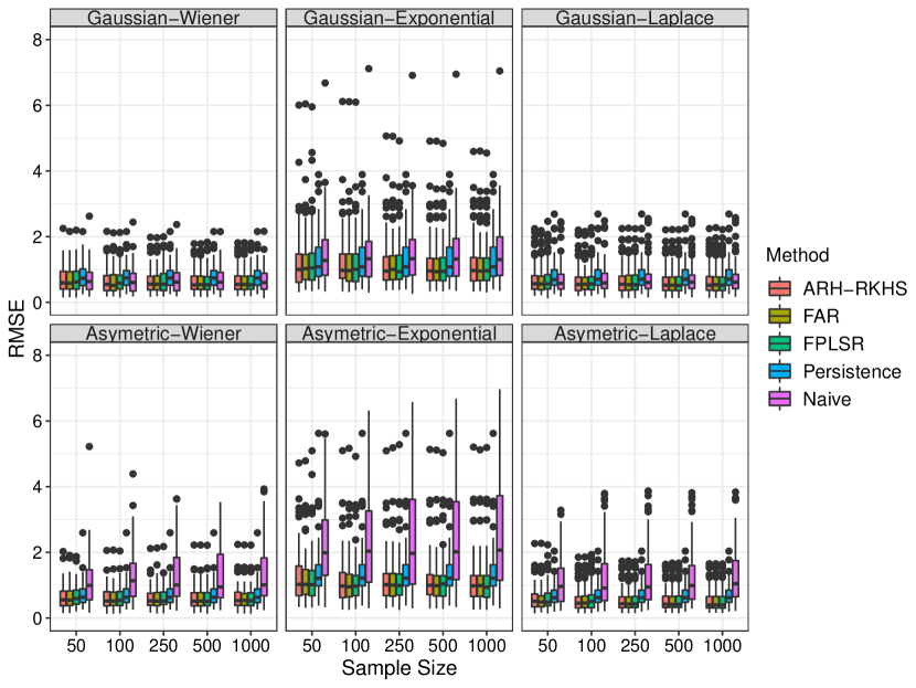
Figure 2: Monte Carlo Results: RMSE distribution by prediction method and simulation setting, throughout a variation of the sample size from 50 to 1000.

Figure 3: Monte Carlo experiment: mean empirical coverage and median amplitude for the different simulations settings, target coverages, band construction methods and sample sizes; 500 MC replications.

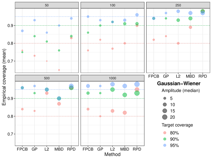
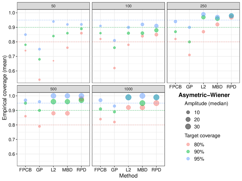
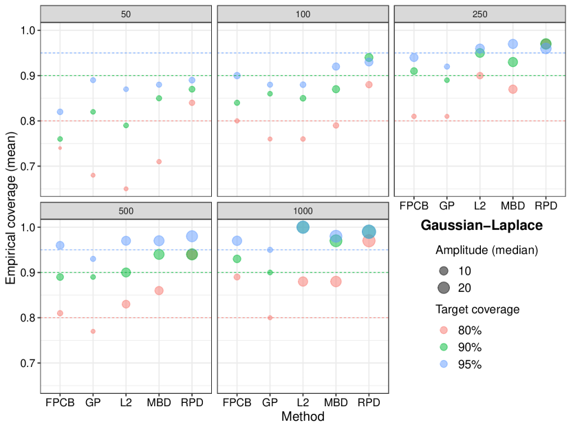
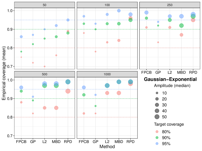
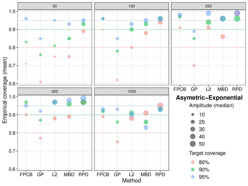
4.2 Experiments on Non-Linear Functional Time Series simulations

Our contribution mainly addresses the construction of the band once a prediction method was chosen and an appropriate bootstrap scheme was used. In the previous experiment, an ARH model was used for both simulation and prediction, and consequently the results are very good both from pointwise and simultaneous prediction point of views. Now, data are simulated according a non-linear generation process. As expected, in this case the ARH-based prediction model will provide bad prediction, and consequently the confidence band based on this bad prediction will not be too wide. But the combination of the proposed band construction with a prediction model adapted to the data generating process, provides much better results.

Simulation setting

For this experiment, data are simulated as in Antoniadis et al., (2006), where the authors propose a non-linear functional time series:

$$X(t)=\beta_{1}m_{1}(t)+\beta_{2}m_{2}(t)+\epsilon(t),$$

where $m_{1}=\cos(2\pi t/64)+\sin(2\pi t/64)$ and $m_{2}=\cos(2\pi t/6)+\sin(2\pi t/6)$, with $\epsilon_{t}\sim$MA(1) a moving average of length 1. The process is then discretized and ends up in $n$ segments of length 64 each (in total $n\times 64$ time points). We set the following values for the parameters : $\beta_{1}=0.8,\beta_{2}=0.18$, the coefficient of the moving average component is 0.8 and the standard deviation of the noise is 0.61. All the parameters were taken from Antoniadis et al., (2006), except from the last one which was optimized in order to match the signal-to-noise ratio of this experiment to the one in Section 4.1.

Results

Table 1 presents the coverage and amplitude results for the FPCB bands, constructed either with the ARH-RKHS predictor and with the Functional Kernel Wavelet predictor (FKW, Antoniadis et al., (2006)). The idea of FKW is to look for patterns in the past data that are similar to the last observed curve. Then, the prediction is a weighed mean of past curves, where weights increase with the similarity between the current and past contexts. The predictor is written as

$$\widehat{Z}_{n+1}=\sum_{m=2}^{n}w_{n,m-1}Z_{m-1}(t),$$

where $w_{n,m-1}$ measures the similarity between the curves $n$ and $m-1$ for every curve in the past. Note that the weights are computed between the $n$ and $m$-th curves, but the next one (i.e. $m+1$) enters into the predictor. We ran an experiment using 500 MC replicates with the calibration levels obtained before. The nominal coverage levels were still reached, but this time with narrower intervals.

With the ARH-RKHS predictor, the coverage of the bands are, as expected, too high with respect to the nominal levels. Unsurprisingly, this behaviour is obtained given the that the amplitude of the bands is too large. With the FKW predictor, the empirical coverage levels are lower than those obtained with the linear method (ARH-RKHS), although they reach the nominal values. Moreover, these coverage levels are achieved with bands that are on average 7.5 times narrower. This shows that making inferences with the method proposed in this paper can be efficient regardless of the predictor used, as long as it is efficient.

Table 1: Coverage and amplitude for the FPCB bands constructed using an ARH-RKHS predictor on a non linear functional time series.

Method	Nominal 80%			Nominal 90%			Nominal 95%
	Cov.	Cov. (pointwise)	Amp.	Cov.	Cov. (pointwise)	Amp.	Cov.	Cov. (pointwise)	Amp.
fpcb-ARH-RKHS	96%	99.86%	7.01	98%	99.90%	11.63	98.8%	99.90%	19.20
fpcb-FKW	89%	99.75%	1.63	94%	99.89%	1.68	95%	99.90%	1.72

4.3 Real data application

We illustrate our proposed methodology with the Particulate Matter Concentrations dataset available in R-package ‘ftsa’. The data consist of 182 daily curves that measure the concentrations (measured in ug/m3) of particular matter with an aerodynamic diameter of less than 10um (PM10) and half-hourly sampled and taken in Graz-Mitte, Austria from October 1, 2010 until March 31, 2011. A square root transformation is applied in order to stabilize the variance.

For this experiment, we divide the sample in the usual training-validation-testing fashion (60%-20%-20%). Given the sample size, we use 110 curves to train, 36 to validate the parameters, and 36 curves for testing. This means we have a forecasting horizon of 36 days, where each forecast is obtained with a one-step-ahead predictor, e.g., the prediction at N+h is conditional to the information at N+h-1. For this experiment, the value of the kernel parameter $\sigma$ is 1 and 7 basis functions were used for all the estimation methods.

The results are presented in Figure 4 and Table 2. In terms of the accuracy of the prediction methods, it can be seen that our proposed model shows a lower RMSE, even if the difference among the functional methods is not statistically significant. However, any of the functional methods improve the quality of the forecast with respect to the persistence and historic mean prediction. The coverage and amplitude results show that the fpcb method offers solid results to make inference. In the three scenarios stated, the fpcb method achieves the desired nominal levels of confidence. This desired confidence level is obtained with wider bands; for a nominal coverage of 95% the fpcb method is, on average, 30% wider than the depth-based alternative procedures. The distance-based competitor ($L_{2}$) presents a good performance in terms of coverage (comparable in some cases with the fpcb method) but with the cost of constructing wider bands.

Finally, we will comment on the shape of the fpcb bands as illustrated in the right panel of Figure 4. The target function (black-dashed line) has a form presenting clearly two peaks which are usually associated to traffic rush in the morning and the afternoon. Note that these peaks reflects the behaviour of economic and social patterns and are impacted by the calendar. That is, they may present shifts during the year, caused by time-saving local rules and are more clear during working days than weekends. The prediction has a much smoother shape. Indeed, we aim to estimate the (non-statistical) predictor $\widetilde{Z}_{n+1|n}$ since this is the best we can manage with the information given until moment $n$. Naturally, the band we construct also inherits this constraint, which explains the much smoother behaviour with respect to the datum $Z_{n+1}$.

Figure 4: PM10 data set: RMSE distribution by prediction method (left); fpcb predictive confidence bands for different confidence levels (right).

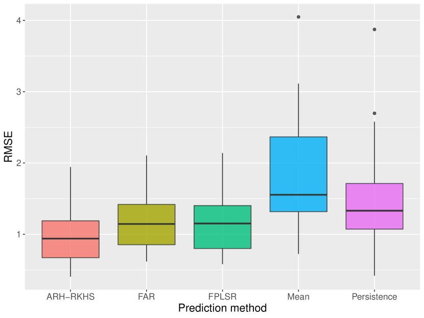
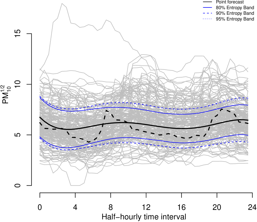
Table 2: PM10 data set: average coverages and amplitude for different nominal coverages ($1-\alpha$), band construction methods and sample sizes; forecast horizon = 36.

Method	Nominal 80%			Nominal 90%			Nominal 95%
	Cov.	Cov. (pointwise)	Amp.	Cov.	Cov. (pointwise)	Amp.	Cov.	Cov. (pointwise)	Amp.
fpcb	89%	99%	9.17	92%	100%	9.95	95%	100%	10.39
MBD	56%	83%	6.21	69%	89%	7.49	75%	93%	8.30
RPD	58%	84%	6.27	67%	91%	7.78	78%	94%	8.86
$L_{2}$	89%	99%	10.63	86%	98%	10.61	83%	98%	10.66
$GP$	97%	99%	9.85	100%	100%	11.28	100%	100%	12.68

5 Concluding comments

In this paper, we present a novel method for constructing simultaneous confidence bands for the prediction of a functional time series data set, based on an entropy measure for stochastic processes. To construct predictive bands we use a functional version of residual bootstrap that allow us to estimate the prediction law through the use of pseudo-predictions. Each pseudo-realisation is then projected into a space of finite dimension, associated to a functional basis, where the $1-\alpha-$MES are obtained. We map the minimum entropy set back to the functional space and construct a band using the regularity of the RKHS. Through a Monte Carlo study, we show the performance of the proposed model in terms of the accuracy, coverage and amplitude, against other prediction methodologies and band construction techniques for functional time series. To illustrate the procedure through a real data set, an example of particulate matter concentrations is presented. We focus on one-step-ahead predictions for sake of simplicity. Our approach can be applied for horizons $h>1$ if a prediction method and a bootstrap scheme are available for such prediction horizons. Our simulation study demonstrated that the entropy procedure offers a better coverage which improves (reaching in some cases the nominal value) as the sample sizes increases. For both numerical experiments, our proposed method for the band construction achieves a good compromise between coverage and efficiency, the latter measured through the bandwidth.

While two different bootstrap schemes were used, they rely on prediction methods only through some parameters (i.e. $\hat{\mu}$ and $\Psi$ for the ARH-RKHS model; or $w_{n,m}$ for the non-linear predictor). An interesting perspective for further work would be to use the approach of Paparoditis et al., (2018), which relies on the conditional distribution of the one-step ahead estimator $\hat{Z}_{n+1|n}$.

A key aspect of our method is the construction of the band using a convex hull, as defined in Eq. (17). This implies that the band is compact, leaving aside non-connected configurations. If that were the case, our construction would result in wider bands than the optimal ones. Of course, such situations may arise in practice, for instance if the functional time series presents different regimes or seasonal patterns. Indeed, these non-linear or non-stationary settings need more intrincate constructions that may be investigated in future work.

An important connection with more classical time series can be made. Actually, prediction on FTS can be viewed as simultaneous multi-step-ahead prediction, even in the case where the one-step-ahead function is computed. Take, for instance, the case in section 4.3. Since each function covers 48 single time points, the FTS approach produces a simultaneous forecast for 48 different horizons. Our approach to computing prediction bands is therefore easily adapted to the construction of prediction intervals for several horizons simultaneously. This is the case for instance in Staszewska-Bystrova, (2011) where simultaneous prediction bands are constructed for the trajectories of an impulse-response effect on vector autoregressive processes. Also in Wolf and Wunderli, (2015), the problem is studied from the perspective of joint prediction regions. A comparison of these approaches is given, within the framework of non linear and non stationary FTS in Antoniadis et al., (2016).

Declarations

Conflicts of interest: None of the authors has a conflict of interest.

Ethics approval: Authors have no affiliations with or involvement in any organisation or entity with any financial interest or non-financial interest in the subject matter or materials discussed in this manuscript.

Consent for publication: Authors give consent for publication.

Availability of data and code: Data is available in R-package ‘ftsa’. and source code to reproduce the results is included as a supplementary file in the submission.

Authors’ contributions: Authors contributed equally to this work.

Appendix A Additional results

We present here the detailed results for the experiment in Section 4.1.

Table 3: Monte Carlo experiment. Setting: Gaussian kernel and Wiener noise. Metrics: Mean and standard deviation for simultaneous coverage and point coverage. Mean, median and standard deviation for amplitude. –Results for different target coverages, band construction methods and sample sizes; 500 MC replications.–

Sample Size	Metrics	Entropy			GPs			MBD			RPD			L2
		80%	90%	95%	80%	90%	95%	80%	90%	95%	80%	90%	95%	80%	90%	95%
N = 50	Sim. Cov.	0.760	0.750	0.870	0.730	0.840	0.930	0.650	0.760	0.900	0.830	0.840	0.940	0.700	0.810	0.860
		0.430	0.440	0.340	0.450	0.370	0.260	0.480	0.430	0.300	0.380	0.370	0.240	0.460	0.390	0.350
	Point Cov	0.910	0.920	0.950	0.940	0.980	0.990	0.870	0.900	0.970	0.940	0.940	0.980	0.900	0.930	0.960
		0.200	0.180	0.170	0.140	0.090	0.070	0.260	0.220	0.130	0.170	0.160	0.090	0.200	0.180	0.140
	Amplitude	3.340	3.810	5.590	3.060	3.570	3.980	3.350	4.570	4.570	5.550	5.580	5.580	3.110	3.910	3.910
		2.780	3.110	4.610	3.050	3.560	3.970	2.820	3.520	3.520	4.240	4.530	4.530	2.670	3.530	3.530
		1.620	1.970	4.000	0.330	0.440	0.520	1.930	4.980	4.980	6.820	6.370	6.370	1.420	1.910	1.910
N = 100	Sim. Cov.	0.760	0.860	0.950	0.820	0.900	0.930	0.800	0.910	0.930	0.900	0.910	0.960	0.770	0.920	0.920
		0.430	0.350	0.220	0.390	0.300	0.260	0.400	0.290	0.260	0.300	0.290	0.200	0.420	0.270	0.270
	Point Cov	0.920	0.950	0.980	0.960	0.980	0.990	0.930	0.970	0.970	0.980	0.970	0.990	0.940	0.960	0.980
		0.190	0.150	0.120	0.110	0.090	0.070	0.180	0.120	0.120	0.090	0.100	0.060	0.160	0.130	0.090
	Amplitude	3.580	4.170	6.900	3.140	3.660	4.090	7.520	11.250	11.250	11.070	14.420	14.420	3.970	7.050	7.050
		3.110	3.530	4.540	3.120	3.660	4.090	3.930	6.560	6.560	5.630	7.230	7.230	3.530	4.480	4.480
		1.880	2.030	11.090	0.240	0.300	0.360	9.240	16.320	16.320	14.500	17.780	17.780	1.980	9.700	9.700
N = 250	Sim. Cov.	0.820	0.940	0.940	0.840	0.940	0.970	0.890	0.940	0.970	0.980	0.980	0.970	0.800	0.930	0.980
		0.390	0.240	0.240	0.370	0.240	0.170	0.310	0.240	0.170	0.140	0.140	0.170	0.400	0.260	0.140
	Point Cov	0.940	0.980	0.980	0.970	0.990	0.990	0.950	0.980	0.990	0.990	0.990	0.990	0.900	0.970	0.990
		0.170	0.100	0.100	0.100	0.070	0.070	0.160	0.090	0.060	0.100	0.060	0.060	0.270	0.150	0.050
	Amplitude	4.100	7.000	10.300	3.180	3.720	4.160	10.930	14.760	14.760	17.680	20.720	20.720	6.030	10.210	10.210
		3.660	5.130	7.030	3.170	3.680	4.130	6.960	11.020	11.020	10.180	13.120	13.120	4.780	8.130	8.130
		2.400	6.830	11.900	0.190	0.240	0.270	11.180	13.290	13.290	23.040	24.240	24.240	4.600	7.460	7.460
N = 500	Sim. Cov.	0.840	0.960	0.960	0.830	0.930	0.970	0.870	0.900	0.900	0.960	0.960	0.970	0.930	0.950	0.950
		0.370	0.200	0.200	0.380	0.260	0.170	0.340	0.300	0.300	0.200	0.200	0.170	0.260	0.220	0.220
	Point Cov	0.950	0.980	0.980	0.980	0.990	1.000	0.950	0.960	0.970	0.980	0.980	0.990	0.970	0.980	0.980
		0.150	0.110	0.110	0.080	0.060	0.030	0.160	0.150	0.130	0.120	0.120	0.070	0.150	0.120	0.110
	Amplitude	5.370	7.640	13.470	3.170	3.690	4.160	17.230	23.110	23.110	23.200	28.430	28.430	12.770	19.310	19.310
		4.310	5.720	7.340	3.170	3.680	4.150	9.160	11.920	11.920	12.570	15.450	15.450	7.250	11.050	11.050
		4.190	6.100	22.450	0.160	0.210	0.250	27.180	31.950	31.950	36.820	38.530	38.530	20.840	28.460	28.460
N = 1000	Sim. Cov.	0.840	0.930	0.970	0.800	0.930	0.970	0.820	0.920	0.970	0.950	0.930	0.980	0.830	0.950	0.980
		0.370	0.260	0.170	0.400	0.260	0.170	0.390	0.270	0.170	0.220	0.260	0.140	0.380	0.220	0.140
	Point Cov	0.960	0.980	0.990	0.970	0.990	1.000	0.930	0.970	0.990	0.980	0.990	1.000	0.920	0.980	1.000
		0.120	0.070	0.030	0.090	0.060	0.030	0.190	0.110	0.080	0.090	0.060	0.040	0.230	0.110	0.030
	Amplitude	5.540	10.440	14.380	3.180	3.690	4.130	21.680	26.530	26.530	27.960	31.830	31.830	13.380	27.830	27.830
		5.120	6.810	9.700	3.170	3.670	4.100	11.100	14.520	14.520	14.720	21.270	21.270	8.740	14.080	14.080
		3.330	10.500	11.970	0.110	0.160	0.220	25.990	26.460	26.460	29.680	29.650	29.650	14.280	33.280	33.280

Table 4: Monte Carlo experiment. Setting: Gaussian kernel and Laplacian noise. Metrics: Mean and standard deviation for simultaneous coverage and point coverage. Mean, median and standard deviation for amplitude. –Results for different target coverages, band construction methods and sample sizes; 500 MC replications.–

Sample Size	Metrics	Entropy			GPs			MBD			RPD			L2
		80%	90%	95%	80%	90%	95%	80%	90%	95%	80%	90%	95%	80%	90%	95%
N -= 50	Sim. Cov.	0.740	0.760	0.820	0.680	0.820	0.890	0.710	0.850	0.880	0.840	0.870	0.890	0.650	0.790	0.870
		0.440	0.430	0.390	0.470	0.390	0.310	0.460	0.360	0.330	0.370	0.340	0.310	0.480	0.410	0.340
	Point Cov	0.910	0.930	0.940	0.930	0.970	0.990	0.920	0.940	0.950	0.950	0.960	0.970	0.900	0.930	0.950
		0.210	0.170	0.160	0.160	0.100	0.050	0.180	0.170	0.160	0.150	0.120	0.110	0.190	0.190	0.160
	Amplitude	3.320	4.100	8.960	3.130	3.620	4.050	4.240	6.370	6.370	6.140	8.900	8.900	3.250	4.290	4.290
		2.740	3.600	4.650	3.070	3.570	3.970	3.370	4.140	4.140	4.410	4.930	4.930	3.100	3.680	3.680
		1.900	2.360	20.210	0.470	0.570	0.660	3.590	9.510	9.510	7.830	13.540	13.540	1.490	3.340	3.340
N = 100	Sim. Cov.	0.800	0.840	0.900	0.760	0.860	0.880	0.790	0.870	0.920	0.880	0.940	0.930	0.760	0.850	0.880
		0.400	0.370	0.300	0.430	0.350	0.330	0.410	0.340	0.270	0.330	0.240	0.260	0.430	0.360	0.330
	Point Cov	0.930	0.950	0.970	0.930	0.950	0.970	0.940	0.960	0.960	0.960	0.980	0.980	0.920	0.960	0.960
		0.180	0.160	0.130	0.190	0.160	0.130	0.170	0.150	0.150	0.130	0.080	0.100	0.190	0.120	0.140
	Amplitude	3.740	5.940	8.120	3.120	3.620	4.100	7.720	12.010	12.010	10.580	16.570	16.570	4.330	7.720	7.720
		3.300	4.170	5.870	3.130	3.600	4.100	4.460	7.330	7.330	5.720	9.080	9.080	3.470	4.720	4.720
		2.160	4.950	11.470	0.300	0.380	0.460	11.640	16.710	16.710	15.770	24.770	24.770	2.880	10.480	10.480
N = 250	Sim. Cov.	0.810	0.890	0.940	0.810	0.890	0.920	0.870	0.930	0.970	0.970	0.970	0.960	0.900	0.950	0.960
		0.390	0.290	0.240	0.390	0.310	0.270	0.340	0.260	0.170	0.170	0.170	0.200	0.300	0.220	0.200
	Point Cov	0.920	0.970	0.970	0.950	0.960	0.970	0.970	0.970	0.990	1.000	0.990	0.990	0.950	0.980	0.990
		0.210	0.120	0.120	0.170	0.160	0.140	0.110	0.140	0.080	0.020	0.040	0.040	0.170	0.130	0.050
	Amplitude	4.380	7.600	15.600	3.160	3.680	4.120	17.880	23.650	23.650	23.100	30.530	30.530	7.660	17.930	17.930
		3.430	6.450	9.290	3.140	3.660	4.090	9.860	12.430	12.430	13.160	16.660	16.660	5.970	11.330	11.330
		3.090	6.310	20.060	0.230	0.270	0.340	31.680	39.390	39.390	37.740	47.750	47.750	5.490	28.470	28.470
N = 500	Sim. Cov.	0.810	0.900	0.960	0.770	0.890	0.930	0.860	0.940	0.970	0.940	0.940	0.980	0.830	0.900	0.970
		0.390	0.310	0.200	0.420	0.310	0.260	0.350	0.240	0.170	0.240	0.240	0.140	0.380	0.300	0.170
	Point Cov	0.940	0.970	0.980	0.940	0.970	0.980	0.960	0.970	0.990	0.980	0.980	0.990	0.920	0.950	0.990
		0.160	0.130	0.090	0.170	0.120	0.100	0.140	0.120	0.080	0.090	0.080	0.070	0.210	0.160	0.070
	Amplitude	4.810	8.410	15.070	3.170	3.670	4.130	16.150	23.350	23.350	22.870	29.390	29.390	11.050	18.800	18.800
		4.260	6.490	8.700	3.140	3.650	4.090	9.630	15.130	15.130	16.270	18.820	18.820	8.510	11.730	11.730
		2.860	7.620	18.280	0.170	0.220	0.260	19.840	23.750	23.750	24.610	30.220	30.220	10.530	22.130	22.130
N = 1000	Sim. Cov.	0.890	0.930	0.970	0.800	0.900	0.950	0.880	0.970	0.980	0.970	0.990	0.990	0.880	1.000	1.000
		0.310	0.260	0.170	0.400	0.300	0.220	0.330	0.170	0.140	0.170	0.100	0.100	0.330	0.000	0.000
	Point Cov	0.940	0.980	0.990	0.940	0.960	0.970	0.960	1.000	1.000	0.990	1.000	1.000	0.940	1.000	1.000
		0.180	0.100	0.040	0.190	0.160	0.140	0.130	0.030	0.020	0.070	0.010	0.020	0.200	0.000	0.000
	Amplitude	5.990	14.110	20.930	3.180	3.710	4.150	23.950	32.560	32.560	34.350	39.550	39.550	22.260	32.960	32.960
		5.170	8.140	12.940	3.190	3.730	4.130	16.510	22.060	22.060	23.420	28.620	28.620	12.690	23.150	23.150
		4.080	16.390	23.490	0.160	0.200	0.240	22.180	29.630	29.630	33.810	37.110	37.110	26.370	29.640	29.640

Table 5: Monte Carlo experiment. Setting: Gaussian kernel and exponential noise. Metrics: Mean and standard deviation for simultaneous coverage and point coverage. Mean, median and standard deviation for amplitude. –Results for different target coverages, band construction methods and sample sizes; 500 MC replications.–

Sample Size	Metrics	Entropy			GPs			MBD			RPD			L2
		80%	90%	95%	80%	90%	95%	80%	90%	95%	80%	90%	95%	80%	90%	95%
N = 50	Sim. Cov.	0.750	0.780	0.860	0.720	0.820	0.870	0.760	0.860	0.920	0.890	0.880	0.950	0.700	0.850	0.900
		0.440	0.420	0.350	0.450	0.390	0.340	0.430	0.350	0.270	0.310	0.330	0.220	0.460	0.360	0.300
	Point Cov	0.920	0.930	0.940	0.930	0.960	0.970	0.930	0.960	0.970	0.980	0.970	0.980	0.910	0.960	0.970
		0.190	0.170	0.170	0.170	0.130	0.120	0.160	0.110	0.130	0.070	0.110	0.110	0.200	0.130	0.110
	Amplitude	12.030	17.140	47.030	6.070	7.090	7.940	25.860	37.030	37.030	38.970	49.080	49.080	10.240	18.890	18.890
		5.740	6.440	14.680	6.050	7.080	7.850	6.710	13.990	13.990	10.440	16.150	16.150	6.110	7.450	7.450
		34.500	38.240	90.740	0.910	1.170	1.410	54.450	63.660	63.660	76.450	85.830	85.830	31.110	43.240	43.240
N = 100	Sim. Cov.	0.880	0.930	0.970	0.780	0.900	0.930	0.840	0.930	1.000	0.960	0.950	0.980	0.830	0.930	0.980
		0.330	0.260	0.170	0.420	0.300	0.260	0.370	0.260	0.000	0.200	0.220	0.140	0.380	0.260	0.140
	Point Cov	0.970	0.980	0.990	0.960	0.980	0.980	0.950	0.980	1.000	0.980	0.990	1.000	0.930	0.980	0.990
		0.120	0.110	0.040	0.140	0.100	0.070	0.170	0.090	0.000	0.090	0.060	0.030	0.200	0.120	0.090
	Amplitude	9.940	20.680	27.600	6.260	7.230	8.100	32.720	45.080	45.080	55.520	55.620	55.620	13.520	28.710	28.710
		6.270	9.850	11.190	6.240	7.200	8.040	15.930	22.500	22.500	29.420	32.330	32.330	8.900	15.530	15.530
		11.290	39.080	43.410	0.680	0.850	0.950	45.450	60.280	60.280	75.620	66.320	66.320	16.960	39.940	39.940
N = 250	Sim. Cov.	0.910	0.960	0.990	0.830	0.920	0.940	0.870	0.920	0.970	0.950	0.970	0.980	0.910	0.950	0.970
		0.290	0.200	0.100	0.380	0.270	0.240	0.340	0.270	0.170	0.220	0.170	0.140	0.290	0.220	0.170
	Point Cov	0.970	0.980	1.000	0.960	0.970	0.980	0.960	0.970	0.990	0.990	0.990	0.990	0.970	0.990	0.990
		0.120	0.110	0.050	0.160	0.150	0.140	0.140	0.120	0.080	0.060	0.040	0.050	0.140	0.040	0.040
	Amplitude	12.680	28.230	47.180	6.350	7.390	8.210	43.650	66.130	66.130	65.620	81.350	81.350	30.350	53.880	53.880
		9.860	16.980	32.120	6.360	7.390	8.190	23.440	41.270	41.270	38.040	52.180	52.180	14.810	29.130	29.130
		9.710	36.710	46.630	0.470	0.630	0.710	57.930	77.480	77.480	78.150	95.340	95.340	54.330	76.100	76.100
N = 500	Sim. Cov.	0.880	0.940	0.960	0.820	0.890	0.910	0.850	0.970	0.980	0.940	0.990	0.990	0.850	0.970	0.980
		0.330	0.240	0.200	0.390	0.310	0.290	0.360	0.170	0.140	0.240	0.100	0.100	0.360	0.170	0.140
	Point Cov	0.950	0.980	0.980	0.960	0.980	0.980	0.950	0.990	0.990	0.980	1.000	1.000	0.940	1.000	0.990
		0.150	0.100	0.100	0.120	0.090	0.070	0.160	0.060	0.060	0.130	0.020	0.050	0.190	0.020	0.070
	Amplitude	17.640	30.670	45.920	6.340	7.350	8.200	50.620	65.860	65.860	71.090	76.820	76.820	38.650	68.920	68.920
		9.520	15.290	26.940	6.330	7.320	8.210	34.260	49.520	49.520	52.690	55.320	55.320	21.780	47.190	47.190
		28.170	40.000	48.550	0.380	0.450	0.540	45.890	51.750	51.750	60.120	62.330	62.330	42.530	77.280	77.280
N = 1000	Sim. Cov.	0.820	0.920	0.960	0.820	0.860	0.920	0.930	0.990	0.990	0.980	0.990	0.990	0.930	0.970	0.970
		0.390	0.270	0.200	0.390	0.350	0.270	0.260	0.100	0.100	0.140	0.100	0.100	0.260	0.170	0.170
	Point Cov	0.940	0.960	0.980	0.950	0.970	0.980	0.980	0.990	0.990	1.000	1.000	1.000	0.950	0.990	0.980
		0.160	0.150	0.090	0.160	0.120	0.100	0.100	0.070	0.070	0.040	0.040	0.050	0.200	0.050	0.120
	Amplitude	16.240	28.990	41.420	6.360	7.400	8.250	55.700	69.560	69.560	74.730	84.450	84.450	57.360	69.370	69.370
		10.040	19.030	27.620	6.350	7.410	8.200	37.810	44.280	44.280	46.120	51.040	51.040	30.160	48.280	48.280
		15.960	31.960	41.060	0.350	0.420	0.490	60.770	75.270	75.270	87.750	99.060	99.060	73.220	73.900	73.900

Table 6: Monte Carlo experiment. Setting: asymmetric kernel and Wiener noise. Metrics: Mean and standard deviation for simultaneous coverage and point coverage. Mean, median and standard deviation for amplitude. –Results for different target coverages, band construction methods and sample sizes; 500 MC replications.–

Sample Size	Metrics	Entropy			GPs			MBD			RPD			L2
		80%	90%	95%	80%	90%	95%	80%	90%	95%	80%	90%	95%	80%	90%	95%
N = 50	Sim. Cov.	0.740	0.780	0.850	0.540	0.680	0.750	0.760	0.860	0.920	0.860	0.890	0.920	0.670	0.840	0.940
		0.440	0.420	0.360	0.500	0.470	0.440	0.430	0.350	0.270	0.350	0.310	0.270	0.470	0.370	0.240
	Point Cov	0.910	0.940	0.970	0.790	0.870	0.920	0.940	0.950	0.980	0.960	0.980	0.980	0.910	0.960	0.990
		0.190	0.150	0.090	0.310	0.260	0.220	0.160	0.160	0.100	0.130	0.100	0.090	0.190	0.130	0.070
	Amplitude	3.350	4.380	8.090	3.930	4.680	5.300	5.290	6.420	6.420	7.910	7.760	7.760	3.690	4.780	4.780
		3.150	3.910	4.750	3.780	4.520	5.180	4.120	4.550	4.550	5.020	5.190	5.190	3.000	4.420	4.420
		1.790	2.980	13.730	0.830	1.060	1.230	6.520	7.860	7.860	10.880	8.970	8.970	2.170	2.430	2.430
N = 100	Sim. Cov.	0.820	0.860	0.910	0.620	0.760	0.810	0.840	0.860	0.920	0.850	0.880	0.910	0.780	0.860	0.900
		0.390	0.350	0.290	0.490	0.430	0.390	0.370	0.350	0.270	0.360	0.330	0.290	0.420	0.350	0.300
	Point Cov	0.930	0.960	0.970	0.810	0.870	0.900	0.930	0.960	0.980	0.960	0.960	0.980	0.920	0.970	0.970
		0.180	0.130	0.120	0.330	0.290	0.260	0.200	0.140	0.080	0.170	0.150	0.100	0.210	0.120	0.140
	Amplitude	3.690	4.700	6.250	4.390	5.250	5.990	13.680	16.780	16.780	21.720	22.400	22.400	6.910	15.360	15.360
		3.440	4.030	4.320	4.320	5.080	5.750	6.420	9.370	9.370	9.900	14.300	14.300	4.110	6.670	6.670
		1.950	2.630	6.960	0.750	0.970	1.180	23.170	24.930	24.930	37.900	32.080	32.080	10.460	28.820	28.820
N = 250	Sim. Cov.	0.820	0.870	0.940	0.710	0.800	0.900	0.920	0.960	0.970	0.970	0.980	0.980	0.870	0.970	0.990
		0.390	0.340	0.240	0.460	0.400	0.300	0.270	0.200	0.170	0.170	0.140	0.140	0.340	0.170	0.100
	Point Cov	0.940	0.950	0.970	0.850	0.910	0.950	0.960	1.000	1.000	0.980	1.000	1.000	0.950	0.990	1.000
		0.150	0.170	0.120	0.310	0.240	0.200	0.140	0.020	0.020	0.130	0.010	0.010	0.190	0.080	0.000
	Amplitude	4.160	6.680	11.240	4.880	5.870	6.720	26.440	34.950	34.950	36.030	42.520	42.520	22.440	35.500	35.500
		3.790	5.360	8.220	4.810	5.720	6.700	11.840	18.080	18.080	17.310	22.140	22.140	7.960	15.490	15.490
		2.090	5.040	9.260	0.770	0.950	1.140	38.300	49.200	49.200	48.780	55.490	55.490	41.900	55.600	55.600
N = 500	Sim. Cov.	0.860	0.950	0.970	0.790	0.900	0.960	0.880	0.960	1.000	0.980	0.970	1.000	0.880	0.960	1.000
		0.350	0.220	0.170	0.410	0.300	0.200	0.330	0.200	0.000	0.140	0.170	0.000	0.330	0.200	0.000
	Point Cov	0.960	0.990	0.990	0.910	0.960	0.980	0.960	0.990	1.000	0.990	0.990	1.000	0.950	1.000	1.000
		0.130	0.050	0.070	0.220	0.150	0.100	0.120	0.080	0.000	0.060	0.060	0.000	0.170	0.020	0.000
	Amplitude	4.990	8.530	11.780	5.010	6.050	6.860	29.670	35.000	35.000	37.960	41.320	41.320	26.840	40.620	40.620
		4.070	6.610	8.020	4.940	6.020	6.860	17.510	24.040	24.040	24.080	26.830	26.830	13.750	26.690	26.690
		3.430	6.570	14.880	0.500	0.630	0.750	30.160	34.510	34.510	37.960	39.580	39.580	32.730	39.730	39.730
N = 1000	Sim. Cov.	0.840	0.910	0.970	0.820	0.890	0.930	0.920	0.950	1.000	0.950	0.990	0.990	0.920	0.990	0.990
		0.370	0.290	0.170	0.390	0.310	0.260	0.270	0.220	0.000	0.220	0.100	0.100	0.270	0.100	0.100
	Point Cov	0.950	0.980	0.990	0.890	0.950	0.970	0.980	0.990	1.000	0.990	1.000	1.000	0.970	1.000	1.000
		0.120	0.090	0.030	0.280	0.180	0.140	0.090	0.080	0.000	0.060	0.040	0.020	0.140	0.000	0.050
	Amplitude	5.320	8.950	15.810	5.040	6.090	6.990	34.270	43.080	43.080	43.930	48.750	48.750	37.660	49.310	49.310
		4.730	6.850	11.210	5.020	6.090	6.920	24.030	30.150	30.150	31.040	33.820	33.820	18.910	34.740	34.740
		3.190	7.770	13.710	0.420	0.560	0.680	34.970	41.830	41.830	43.830	45.750	45.750	46.930	46.400	46.400

Table 7: Monte Carlo experiment. Setting: asymmetric kernel and Laplacian noise. Metrics: Mean and standard deviation for simultaneous coverage and point coverage. Mean, median and standard deviation for amplitude. –Results for different target coverages, band construction methods and sample sizes; 500 MC replications.–

Sample Size	Metrics	Entropy			GPs			MBD			RPD			L2
		80%	90%	95%	80%	90%	95%	80%	90%	95%	80%	90%	95%	80%	90%	95%
N = 50	Sim. Cov.	0.760	0.810	0.910	0.550	0.690	0.860	0.800	0.850	0.960	0.850	0.930	0.950	0.760	0.820	0.930
		0.430	0.390	0.290	0.500	0.460	0.350	0.400	0.360	0.200	0.360	0.260	0.220	0.430	0.390	0.260
	Point Cov	0.920	0.960	0.970	0.790	0.880	0.920	0.940	0.950	0.980	0.960	0.980	0.980	0.920	0.950	0.990
		0.180	0.120	0.130	0.330	0.290	0.240	0.190	0.170	0.140	0.130	0.110	0.100	0.190	0.170	0.050
	Amplitude	3.470	4.180	7.050	3.840	4.540	5.150	7.520	10.300	10.300	8.520	13.130	13.130	3.540	5.170	5.170
		3.050	3.640	4.580	3.830	4.470	5.040	3.920	4.680	4.680	4.440	5.360	5.360	3.230	4.670	4.670
		1.750	2.280	9.030	0.710	0.900	1.060	15.910	21.250	21.250	20.590	26.270	26.270	1.760	5.350	5.350
N = 100	Sim. Cov.	0.800	0.910	0.920	0.650	0.740	0.830	0.790	0.910	0.910	0.830	0.950	0.960	0.810	0.890	0.940
		0.400	0.290	0.270	0.480	0.440	0.380	0.410	0.290	0.290	0.380	0.220	0.200	0.390	0.310	0.240
	Point Cov	0.940	0.960	0.970	0.790	0.880	0.920	0.910	0.950	0.960	0.950	0.970	0.970	0.920	0.950	0.970
		0.160	0.160	0.140	0.340	0.260	0.230	0.230	0.200	0.170	0.160	0.140	0.150	0.220	0.200	0.160
	Amplitude	3.800	5.830	7.620	4.470	5.360	6.090	9.670	21.470	21.470	17.030	26.480	26.480	7.830	14.980	14.980
		3.190	4.510	5.560	4.340	5.130	5.750	4.270	9.260	9.260	5.180	10.610	10.610	3.680	6.180	6.180
		2.570	4.560	6.720	0.910	1.140	1.350	13.020	34.060	34.060	29.360	36.440	36.440	16.270	19.690	19.690
N = 250	Sim. Cov.	0.810	0.920	0.960	0.680	0.850	0.910	0.880	0.950	0.980	0.950	0.960	0.980	0.880	0.930	1.000
		0.390	0.270	0.200	0.470	0.360	0.290	0.330	0.220	0.140	0.220	0.200	0.140	0.330	0.260	0.000
	Point Cov	0.910	0.960	0.990	0.880	0.940	0.960	0.950	0.970	0.990	0.970	0.980	0.990	0.960	0.960	1.000
		0.220	0.150	0.080	0.250	0.210	0.180	0.200	0.140	0.070	0.140	0.120	0.050	0.160	0.190	0.000
	Amplitude	4.510	7.660	16.620	4.750	5.720	6.560	19.200	23.590	23.590	28.520	29.070	29.070	12.830	24.600	24.600
		3.410	5.530	10.180	4.600	5.550	6.400	11.010	13.530	13.530	15.080	16.490	16.490	7.640	14.710	14.710
		3.000	6.940	21.260	0.650	0.820	1.040	27.020	30.770	30.770	40.240	37.460	37.460	14.590	34.750	34.750
N = 500	Sim. Cov.	0.860	0.930	0.980	0.770	0.860	0.920	0.860	0.900	0.980	0.940	0.960	0.980	0.780	0.930	0.980
		0.350	0.260	0.140	0.420	0.350	0.270	0.350	0.300	0.140	0.240	0.200	0.140	0.420	0.260	0.140
	Point Cov	0.960	0.970	0.990	0.890	0.950	0.980	0.920	0.950	0.980	0.950	0.980	0.990	0.900	0.960	0.990
		0.140	0.120	0.090	0.250	0.160	0.130	0.250	0.180	0.120	0.200	0.120	0.110	0.240	0.150	0.080
	Amplitude	5.320	9.070	14.460	4.940	5.920	6.790	27.700	40.010	40.010	37.430	48.240	48.240	32.020	44.500	44.500
		4.250	6.800	8.850	4.900	5.860	6.720	19.150	25.610	25.610	23.450	35.050	35.050	13.900	28.540	28.540
		4.680	7.990	18.040	0.520	0.610	0.750	30.010	44.220	44.220	39.330	48.390	48.390	58.140	51.570	51.570
N = 1000	Sim. Cov.	0.880	0.920	0.970	0.840	0.940	0.990	0.950	0.970	0.990	0.980	0.980	0.990	0.910	0.990	0.990
		0.330	0.270	0.170	0.370	0.240	0.100	0.220	0.170	0.100	0.140	0.140	0.100	0.290	0.100	0.100
	Point Cov	0.970	0.970	0.990	0.940	0.980	0.990	0.980	0.980	1.000	0.990	0.990	1.000	0.940	0.990	1.000
		0.100	0.110	0.090	0.180	0.100	0.100	0.130	0.110	0.050	0.100	0.090	0.010	0.220	0.100	0.030
	Amplitude	5.750	9.080	17.580	5.020	6.060	6.930	35.390	42.470	42.470	48.070	52.560	52.560	33.770	52.480	52.480
		4.880	6.680	10.970	5.020	5.970	6.820	21.370	31.780	31.780	30.930	36.350	36.350	18.640	34.080	34.080
		3.920	8.770	19.080	0.410	0.510	0.650	39.480	41.790	41.790	52.910	52.120	52.120	43.760	58.330	58.330

Table 8: Monte Carlo experiment. Setting: asymmetric kernel and exponential noise. Metrics: Mean and standard deviation for simultaneous coverage and point coverage. Mean, median and standard deviation for amplitude. –Results for different target coverages, band construction methods and sample sizes; 500 MC replications.–

Sample Size	Metrics	Entropy			GPs			MBD			RPD			L2
		80%	90%	95%	80%	90%	95%	80%	90%	95%	80%	90%	95%	80%	90%	95%
N = 50	Sim. Cov.	0.710	0.830	0.960	0.610	0.760	0.850	0.750	0.850	0.930	0.890	0.930	0.950	0.750	0.810	0.950
		0.460	0.380	0.200	0.490	0.430	0.360	0.440	0.360	0.260	0.310	0.260	0.220	0.440	0.390	0.220
	Point Cov	0.920	0.960	0.990	0.820	0.900	0.930	0.920	0.960	0.970	0.970	0.980	0.980	0.920	0.960	0.990
		0.180	0.130	0.070	0.310	0.240	0.200	0.170	0.130	0.120	0.100	0.100	0.100	0.200	0.110	0.060
	Amplitude	9.960	14.980	29.210	7.820	9.300	10.550	44.820	38.700	38.700	66.660	57.100	57.100	13.100	20.290	20.290
		6.100	7.580	13.670	7.520	8.790	10.000	11.110	15.910	15.910	17.640	23.860	23.860	6.580	7.960	7.960
		17.040	23.410	49.160	1.630	2.040	2.400	168.430	52.500	52.500	213.980	84.730	84.730	24.800	33.500	33.500
N = 100	Sim. Cov.	0.900	0.960	0.960	0.620	0.780	0.850	0.880	0.930	0.950	0.940	0.960	0.960	0.800	0.900	0.930
		0.300	0.200	0.200	0.490	0.420	0.360	0.330	0.260	0.220	0.240	0.200	0.200	0.400	0.300	0.260
	Point Cov	0.980	0.990	0.990	0.810	0.880	0.910	0.950	0.980	0.980	0.980	0.980	0.980	0.920	0.960	0.980
		0.090	0.100	0.050	0.340	0.290	0.250	0.160	0.110	0.110	0.100	0.100	0.080	0.220	0.170	0.090
	Amplitude	9.560	17.790	27.560	8.720	10.440	11.900	46.880	57.450	57.450	77.840	80.400	80.400	23.500	54.050	54.050
		6.020	10.310	13.460	8.590	10.300	11.660	20.750	27.100	27.100	29.730	37.150	37.150	9.810	22.600	22.600
		11.620	17.180	40.640	1.590	2.020	2.360	57.280	66.890	66.890	130.750	117.820	117.820	37.750	88.130	88.130
N = 250	Sim. Cov.	0.910	0.970	0.980	0.700	0.850	0.890	0.860	0.960	0.960	0.990	0.960	0.990	0.910	0.940	0.990
		0.290	0.170	0.140	0.460	0.360	0.310	0.350	0.200	0.200	0.100	0.200	0.100	0.290	0.240	0.100
	Point Cov	0.960	0.990	0.990	0.870	0.930	0.960	0.950	0.990	0.990	1.000	1.000	1.000	0.970	0.970	1.000
		0.160	0.060	0.060	0.280	0.200	0.140	0.160	0.040	0.040	0.020	0.030	0.030	0.140	0.160	0.010
	Amplitude	11.100	26.600	44.290	9.670	11.610	13.240	39.120	57.800	57.800	67.720	72.230	72.230	40.610	57.720	57.720
		8.000	14.800	29.670	9.440	11.400	12.880	27.260	48.070	48.070	52.950	58.890	58.890	20.100	42.460	42.460
		9.290	36.880	44.610	1.400	1.670	2.010	37.310	52.460	52.460	69.710	64.150	64.150	46.900	50.630	50.630
N = 500	Sim. Cov.	0.900	0.970	0.950	0.770	0.870	0.920	0.890	0.960	0.980	0.970	0.970	0.990	0.880	0.970	0.970
		0.300	0.170	0.220	0.420	0.340	0.270	0.310	0.200	0.140	0.170	0.170	0.100	0.330	0.170	0.170
	Point Cov	0.950	0.980	0.980	0.900	0.950	0.960	0.960	0.980	0.990	0.990	0.990	0.990	0.940	0.990	0.980
		0.160	0.090	0.090	0.250	0.190	0.160	0.140	0.110	0.080	0.090	0.090	0.070	0.210	0.080	0.100
	Amplitude	16.390	26.950	44.530	9.990	11.990	13.660	44.050	63.140	63.140	67.260	82.750	82.750	47.110	64.710	64.710
		9.610	14.600	20.380	9.890	11.870	13.460	22.900	37.440	37.440	36.610	51.990	51.990	20.840	36.340	36.340
		28.210	37.270	53.750	1.200	1.520	1.740	58.770	69.620	69.620	84.710	91.080	91.080	75.520	71.890	71.890
N = 1000	Sim. Cov.	0.890	0.920	0.930	0.750	0.860	0.930	0.910	0.860	0.830	0.950	0.930	0.930	0.880	0.910	0.900
		0.310	0.270	0.260	0.440	0.350	0.260	0.290	0.350	0.380	0.220	0.260	0.260	0.330	0.290	0.300
	Point Cov	0.960	0.970	0.970	0.870	0.940	0.960	0.950	0.920	0.900	0.970	0.970	0.970	0.930	0.930	0.930
		0.160	0.130	0.130	0.290	0.200	0.160	0.200	0.240	0.260	0.160	0.150	0.150	0.230	0.220	0.230
	Amplitude	16.050	29.860	38.180	10.110	12.260	13.990	54.180	45.760	45.760	74.160	58.080	58.080	58.490	58.260	58.260
		10.920	17.310	22.320	10.090	12.110	13.700	37.280	28.110	28.110	55.720	36.560	36.560	33.520	33.500	33.500
		15.800	38.600	45.180	0.930	1.240	1.370	51.040	48.080	48.080	67.680	58.080	58.080	61.030	60.660	60.660

References

- Alvarez-Liébana, (2017) Alvarez-Liébana, J. (2017). A review and comparative study on functional time series techniques. arXiv preprint arXiv: 1706.06288.
- Antoniadis et al., (2012) Antoniadis, A., Brossat, X., Cugliari, J., and Poggi, J.-M. (2012). Prévision d’un processus à valeurs fonctionnelles en présence de non stationnarités. application à la consommation d’électricité. Journal de la Société Française de Statistique, 153(2):52–78.
- Antoniadis et al., (2016) Antoniadis, A., Brossat, X., Cugliari, J., and Poggi, J.-M. (2016). A prediction interval for a function-valued forecast model: Application to load forecasting. International Journal of Forecasting, 32(3):939 – 947.
- Antoniadis et al., (2006) Antoniadis, A., Paparoditis, E., and Sapatinas, T. (2006). A functional wavelet–kernel approach for time series prediction. Journal of the Royal Statistical Society: Series B (Statistical Methodology), 68(5):837–857.
- Aue et al., (2015) Aue, A., Norinho, D. D., and Hörmann, S. (2015). On the prediction of stationary functional time series. Journal of the American Statistical Association, 110(509):378–392.
- Berlinet and Thomas-Agnan, (2011) Berlinet, A. and Thomas-Agnan, C. (2011). Reproducing kernel Hilbert spaces in probability and statistics. Springer Science & Business Media.
- Bonnevay et al., (2019) Bonnevay, S., Cugliari, J., and Granger, V. (2019). Predictive maintenance from event logs using wavelet-based features: an industrial application. In International Workshop on Soft Computing Models in Industrial and Environmental Applications, pages 132–141. Springer.
- Bosq, (2000) Bosq, D. (2000). Linear processes in function spaces: theory and applications, volume 149. Springer Science & Business Media.
- Cardot et al., (2013) Cardot, H., Cénac, P., Zitt, P.-A., et al. (2013). Efficient and fast estimation of the geometric median in hilbert spaces with an averaged stochastic gradient algorithm. Bernoulli, 19(1):18–43.
- (10) Chakraborty, A. and Chaudhuri, P. (2014a). The deepest point for distributions in infinite dimensional spaces. Statistical Methodology, 20:27–39.
- (11) Chakraborty, A. and Chaudhuri, P. (2014b). On data depth in infinite dimensional spaces. Annals of the Institute of Statistical Mathematics, 66(2):303–324.
- Chen and Pun, (2019) Chen, Y. and Pun, C. S. (2019). A bootstrap-based kpss test for functional time series. Journal of Multivariate Analysis, 174:104535.
- Cucker and Smale, (2002) Cucker, F. and Smale, S. (2002). On the mathematical foundations of learning. Bulletin of the American Mathematical Society, 39:1–49.
- Cuevas et al., (2007) Cuevas, A., Febrero, M., and Fraiman, R. (2007). Robust estimation and classification for functional data via projection-based depth notions. Computational Statistics, 22(3):481–496.
- Damon and Guillas, (2015) Damon, J. and Guillas, S. (2015). Package ‘far’.
- Degras, (2017) Degras, D. (2017). Simultaneous confidence bands for the mean of functional data. Wiley Interdisciplinary Reviews: Computational Statistics, 9(3):e1397.
- Delaigle et al., (2010) Delaigle, A., Hall, P., et al. (2010). Defining probability density for a distribution of random functions. The Annals of Statistics, 38(2):1171–1193.
- Delaigle et al., (2012) Delaigle, A., Hall, P., et al. (2012). Methodology and theory for partial least squares applied to functional data. Annals of Statistics, 40(1):322–352.
- Didericksen et al., (2012) Didericksen, D., Kokoszka, P., and Zhang, X. (2012). Empirical properties of forecasts with the functional autoregressive model. Computational statistics, 27(2):285–298.
- Febrero-Bande and Oviedo de la Fuente, (2013) Febrero-Bande, M. and Oviedo de la Fuente, M. (2013). Package ‘fda. usc’: Functional data analysis and utilities for statistical computing.
- Fraiman and Muniz, (2001) Fraiman, R. and Muniz, G. (2001). Trimmed means for functional data. Test, 10(2):419–440.
- Franke and Nyarige, (2019) Franke, J. and Nyarige, E. G. (2019). A residual-based bootstrap for functional autoregressions. arXiv preprint arXiv:1905.07635.
- Fresoli et al., (2014) Fresoli, D., Ruiz, E., and Pascual, L. (2014). Bootstrap multi-step forecasts of non-gaussian var models. International Journal of Forecasting.
- Galeano et al., (2015) Galeano, P., Joseph, E., and Lillo, R. E. (2015). The mahalanobis distance for functional data with applications to classification. Technometrics, 57(2):281–291.
- Genovese and Wasserman, (2005) Genovese, C. R. and Wasserman, L. (2005). Confidence sets for nonparametric wavelet regression. The Annals of Statistics, 33(2):698–729.
- Hernández et al., (2021) Hernández, N., Cugliari, J., and Jacques, J. (2021). fpcb: Functional predictive confidence bands.
- Hero, (2007) Hero, A. O. (2007). Geometric entropy minimization (gem) for anomaly detection and localization. In Advances in Neural Information Processing Systems, pages 585–592.
- Hörmann et al., (2010) Hörmann, S., Kokoszka, P., et al. (2010). Weakly dependent functional data. The Annals of Statistics, 38(3):1845–1884.
- Hsing and Eubank, (2015) Hsing, T. and Eubank, R. (2015). Theoretical foundations of functional data analysis, with an introduction to linear operators. John Wiley & Sons.
- Hyndman, (1996) Hyndman, R. J. (1996). Computing and graphing highest density regions. The American Statistician, 50(2):120–126.
- Hyndman and Shang, (2009) Hyndman, R. J. and Shang, H. L. (2009). Forecasting functional time series. Journal of the Korean Statistical Society, 38(3):199–211.
- Hyndman and Shang, (2020) Hyndman, R. J. and Shang, H. L. (2020). Package ‘ftsa’.
- J Mercer, (1909) J Mercer, B. (1909). Xvi. functions of positive and negative type, and their connection the theory of integral equations. Phil. Trans. R. Soc. Lond. A, 209(441-458):415–446.
- Koenker and Bassett Jr, (1978) Koenker, R. and Bassett Jr, G. (1978). Regression quantiles. Econometrica: journal of the Econometric Society, pages 33–50.
- López-Pintado and Romo, (2009) López-Pintado, S. and Romo, J. (2009). On the concept of depth for functional data. Journal of the American Statistical Association, 104(486):718–734.
- Lopez-Pintado and Torrente, (2013) Lopez-Pintado, S. and Torrente, A. (2013). depthtools: Depth tools package.
- Martos et al., (2018) Martos, G., Hernández, N., Muñoz, A., and Moguerza, J. M. (2018). Entropy measures for stochastic processes with applications in functional anomaly detection. Entropy, 20(1):33.
- Martos et al., (2014) Martos, G., Muñoz, A., and González, J. (2014). Generalizing the mahalanobis distance via density kernels. Intelligent Data Analysis, 18(6S):S19–S31.
- Mas and Pumo, (2011) Mas, A. and Pumo, B. (2011). Linear processes for functional data. In The Oxford Handbook of Functional Data, pages 47–71. Oxford Univ. Press.
- Muñoz and González, (2010) Muñoz, A. and González, J. (2010). Representing functional data using support vector machines. Pattern Recognition Letters, 31(6):511–516.
- Muñoz and Moguerza, (2006) Muñoz, A. and Moguerza, J. (2006). Estimation of high-density regions using one-class neighbor machines. IEEE Transactions on Pattern Analysis and Machine Intelligence, 28(3):476–480.
- Nagbe et al., (2018) Nagbe, K., Cugliari, J., and Jacques, J. (2018). Short-term electricity demand forecasting using a functional state space model. Energies, 11(5):1–24.
- Paparoditis et al., (2018) Paparoditis, E. et al. (2018). Sieve bootstrap for functional time series. The Annals of Statistics, 46(6B):3510–3538.
- Paparoditis and Shang, (2020) Paparoditis, E. and Shang, H. L. (2020). Bootstrap prediction bands for functional time series. arXiv preprint arXiv:2004.03971.
- Pascual et al., (2004) Pascual, L., Romo, J., and Ruiz, E. (2004). Bootstrap predictive inference for arima processes. Journal of Time Series Analysis, 25(4):449–465.
- Ramsay, (2006) Ramsay, J. O. (2006). Functional data analysis. Wiley Online Library.
- Rényi et al., (1961) Rényi, A. et al. (1961). On measures of entropy and information. In Proceedings of the Fourth Berkeley Symposium on Mathematical Statistics and Probability, Volume 1: Contributions to the Theory of Statistics, pages 547–561. The Regents of the University of California.
- Shang, (2018) Shang, H. L. (2018). Bootstrap methods for stationary functional time series. Statistics and Computing, 28(1):1–10.
- Shannon, (1948) Shannon, C. E. (1948). A mathematical theory of communication. The Bell system technical journal, 27(3):379–423.
- Staszewska-Bystrova, (2011) Staszewska-Bystrova, A. (2011). Bootstrap prediction bands for forecast paths from vector autoregressive models. Journal of Forecasting, 30(8):721–735.
- Tavakoli et al., (2023) Tavakoli, S., Nisol, G., and Hallin, M. (2023). Factor models for high-dimensional functional time series ii: Estimation and forecasting. Journal of Time Series Analysis.
- Wand and Jones, (1994) Wand, M. P. and Jones, M. C. (1994). Kernel smoothing. Chapman and Hall/CRC.
- Wang et al., (2020) Wang, D., Zhao, Z., Willett, R., and Yau, C. Y. (2020). Functional autoregressive processes in reproducing kernel hilbert spaces. arXiv preprint arXiv:2011.13993.
- Wolf and Wunderli, (2015) Wolf, M. and Wunderli, D. (2015). Bootstrap joint prediction regions. Journal of Time Series Analysis, 36(3):352–376.