A nearly Blackwell-optimal policy gradient method

Abstract

For continuing environments, reinforcement learning (RL) methods commonly maximize the discounted reward criterion with discount factor close to 1 in order to approximate the average reward (the gain). However, such a criterion only considers the long-run steady-state performance, ignoring the transient behaviour in transient states. In this work, we develop a policy gradient method that optimizes the gain, then the bias (which indicates the transient performance and is important to capably select from policies with equal gain). We derive expressions that enable sampling for the gradient of the bias and its preconditioning Fisher matrix. We further devise an algorithm that solves the gain-then-bias (bi-level) optimization. Its key ingredient is an RL-specific logarithmic barrier function. Experimental results provide insights into the fundamental mechanisms of our proposal.

1 Introduction

1.1 A motivating example

Consider an environment in Fig 1, for which any stationary policy $\pi\in\Pi_{\mathrm{S}}$ has equal gain values (the expected long-run average reward in steady-state), namely $v_{g}(\pi)=-1$. Therefore, all stationary policies are gain optimal, satisfying $v_{g}(\pi)\geq v_{g}(\pi^{\prime}),\ \forall\pi,\pi^{\prime}\in\Pi_{\mathrm{S}}$. In this case, the gain optimality (which is equivalent to $(n=-1)$-discount optimality) is underselective because there is no way to discriminate policies based on their gain values. Nonetheless, there exists a more selective optimality criterion that can be obtained by increasing the value of $n$ from $-1$ to $0$ (or greater, if needed) in the family of $n$-discount optimality (puterman_1994_mdp, Ch 10).

Figure 1: A two-state environment with two policies (red and blue actions) whose gains are all equally $-1$ (puterman_1994_mdp, p500). Each edge label indicates a tuple of reward $r$ and transition probability $p$.

For the environment in Fig 1, $(n=0)$-discount optimality is the most selective because its optimal policy, i.e. selecting the red action, is also optimal with respect to all other $n$-discount optimality criteria for all $n>0$. This selectiveness is achieved by considering not only steady-state (gain) but also transient rewards. This selectiveness can also be achieved by $\gamma$-discounted optimality only if the discount factor $\gamma>10/11\approx 0.909$. Such a critical lower threshold for $\gamma$ is difficult to estimate for environments with unknown dynamics. Moreover, finite-precision computation induces an upper threshold such that the discounted value $v_{\gamma}(\pi)$ is numerically not too close to the gain $v_{g}(\pi)$. Otherwise, $(\gamma\approx 1)$-discounted optimality becomes underselective as well since $\lim_{\gamma\to 1}(1-\gamma)v_{\gamma}(\pi)=v_{g}(\pi)$ (puterman_1994_mdp, Corollary 8.2.5).

1.2 An overview of our proposed method

We believe that one always desires the most selective criterion. This can be obtained by solving ($n=|\mathcal{S}|-2$, at most)-discount optimality for some type of environments with a finite state set $\mathcal{S}$, as shown by puterman_1994_mdp. As a first step in leveraging this fact in reinforcement learning (RL), we focus on $(n=0)$-discount optimality, for which we have the notion of nearly-Blackwell optimality as in Def 1.1 below.

Definition 1.1.

A stationary policy $\pi_{b}^{*}\in\Pi_{\mathrm{S}}$ is nearly-Blackwell optimal (nBw-optimal, also termed bias optimal) if it is gain optimal, and in addition

$$v_{b}(\pi_{b}^{*},s)\geq v_{b}(\pi_{g}^{*},s),\quad\forall s\in\mathcal{S},\forall\pi_{g}^{*}\in\Pi_{g}^{*},\quad\text{with}\ \Pi_{g}^{*}\coloneqq\operatorname*{\arg\!\max}_{\pi\in\Pi_{\mathrm{S}}}v_{g}(\pi),\ \text{and the bias value}$$

$$v_{b}(\pi,s)\coloneqq\lim_{t_{\mathrm{max}}\to\infty}\mathbb{E}_{A_{t}\sim\pi(\cdot|s_{t}),S_{t+1}\sim p(\cdot|s_{t},a_{t})}\mathopen{}\mathclose{{}\left[\sum_{t=0}^{t_{\mathrm{max}}-1}\big{(}r(S_{t},A_{t})-v_{g}(\pi)\big{)}\Big{|}S_{0}=s,\pi}\right],$$ (1)

where $v_{g}$ is the gain value and $r$ is a reward function. The above limit is assumed to exist. See blackwell_1962_ddp, Sec 4; feinberg_2002_hmdp, Def 3.1.

To our knowledge, mahadevan_1996_sensitivedo proposed the first (and the only) tabular Q-learning that can obtain nBw-optimal policies through optimizing the family of $n$-discount optimality. It relies on stochastic approximation (SA) to estimate the optimal values of gain $v_{g}^{*}(=v_{-1}^{*})$, bias $v_{b}^{*}(=v_{0}^{*})$, and bias-offset $v_{1}^{*}$. Since those values are in two nested equations, standard SA is not guaranteed to converge, as noted by the author. For other related works in a broader scope, refer to Sec 8.

The main contribution of this paper is the development of a policy gradient method capable of learning nBw-optimal policies in unichain MDPs. A policy gradient method works by maximizing the expected value of a policy with respect to some initial state distribution, i.e. $\mathbb{E}_{\mathring{p}}\mathopen{}\mathclose{{}\left[v(\pi,S_{0})}\right]$. This generally requires stochastic optimization on a non-concave landscape. The gradient ascent update for iteratively solving the optimization is given by

$$\boldsymbol{\theta}\leftarrow\boldsymbol{\theta}+\alpha\ \boldsymbol{C}^{-1}\ \nabla v(\boldsymbol{\theta},s_{0}),\quad\text{ for a parameterized policy $\pi(\boldsymbol{\theta}),\forall\boldsymbol{\theta}\in\Theta=\real{\dim(\boldsymbol{\theta})}$,}$$ (2)

where $\alpha$ is a positive step length, $\boldsymbol{C}\in\real{\dim(\boldsymbol{\theta})\times\dim(\boldsymbol{\theta})}$ is a positive-definite preconditioning matrix, $s_{0}$ is a deterministic initial state (without loss of generality), $\nabla\coloneqq\partial/\partial\boldsymbol{\theta}$, and $v(\boldsymbol{\theta},s_{0})\coloneqq v(\pi(\boldsymbol{\theta}),s_{0})$. Such optimization needs $\pi(\boldsymbol{\theta})$ that is twice continuously differentiable with bounded first and second derivatives, for which $\pi(\boldsymbol{\theta})$ is necessarily a randomized (stochastic) policy.

In essense, our nBw-optimal policy gradient method switches the optimization objective from gain $v_{g}$ to bias $v_{b}$ once the gain optimization is deemed to have converged. This necessitates three novel ingredients, to which we contribute. First is a sampling-based approximator for the (standard, vanilla) gradient of bias (Sec 3). Second is a suitable preconditioning matrix $\boldsymbol{C}$, for which we define the Fisher (information) matrix of bias, leading to natural gradients of bias (Sec 4). Third is an algorithm that utilizes the gradient and Fisher matrix estimates to carry out gain then bias optimization (Sec 5). For solving the induced bi-level optimization, we formulate a logarithmic barrier function that ensures the optimization iterates stay in the gain-optimal region (as prescribed in Def 1.1). The experiment results in Sec 7 provide insights into the fundamental mechanisms of our proposal, as well as comparison with the discounted reward method.

2 Preliminaries

The interaction between an RL agent and its environment is modelled as a Markov decision process (MDP). An MDP induces Markov chains (MCs), one for each stationary policy $\pi$. Each induced MC has a stochastic one-step transition matrix under $\pi$, denoted as $\boldsymbol{P}_{\!\!\pi}$ and of size $|\mathcal{S}|$-by-$|\mathcal{S}|$. Raising it to the $t$-th power gives $\boldsymbol{P}_{\!\!\pi}^{t}$, whose $[s_{0},s_{t}]$-th component indicates the $t$-step transition probability $p_{\pi}^{t}(s_{t}|s_{0})\coloneqq\mathrm{Pr}\{S_{t}=s_{t}|s_{0};\pi\}$. The limiting matrix is defined as $\boldsymbol{P}_{\!\!\pi}^{\star}\coloneqq\lim_{t\to\infty}\boldsymbol{P}_{\!\!\pi}^{t}$, which exists whenever the MC is aperiodic. Since $\boldsymbol{P}_{\!\!\pi}^{\star}\boldsymbol{P}_{\!\!\pi}=\boldsymbol{P}_{\!\!\pi}^{\star}$, its component $p_{\pi}^{\star}(s|s_{0})$ can be interpreted as the stationary (time-invariant) probability of visiting state $s$ when starting in an initial state $s_{0}$. The time $t$ at which such stationarity (equivalently, the limiting state distribution $p^{\star}$) is achieved, at least approximately, is of special interest. For that, the notion of mixing time is defined in Def 2.1 below.

Definition 2.1.

The mixing time, denoted as $t_{\mathrm{mix}}^{\pi}$, is the time required by an MC induced by a policy $\pi$ such that the distance to the stationarity is small (levin_2009_mvmt, Ch 4.5). That is,

$$t_{\mathrm{mix}}^{\pi}(\varepsilon)\coloneqq\min\Big{\{}t:\max_{s_{0}\in\mathcal{S}}\Big{[}\frac{1}{2}\sum_{s\in\mathcal{S}}\big{|}\boldsymbol{P}_{\!\!\pi}^{t}[s_{0},s]-\boldsymbol{P}_{\!\!\pi}^{\star}[s_{0},s]\big{|}\Big{]}\leq\varepsilon\Big{\}},$$

for an arbitrarily small $\varepsilon<1/2$.

We consider an agent-environment interaction whose MDP model satisfies Assumption 2.1 below. We remark that the mixing time (Def 2.1) is commonly specified with a positive $\varepsilon$ in order to quantify some approximation. To suppress such approximation (at least notationally), we idealize the concept of mixing by having $t_{\mathrm{mix}}^{\pi}\coloneqq t_{\mathrm{mix}}^{\pi}(\varepsilon=0)$, i.e. completely mixing. Note that in some MCs, the stationarity is indeed exactly achieved in finite time, hence $t_{\mathrm{mix}}^{\pi}<\infty$. Fig 2 depicts this $t_{\mathrm{mix}}$ milestone on the timestep line of an infinite-horizon MDP.

Assumption 2.1.

The modelling MDP is unichain and aperiodic. Every induced MC has a finite mixing time (Def 2.1), that is $t_{\mathrm{mix}}^{\pi}(\varepsilon)<\infty$.

Figure 2: A diagram for pre-mixing (green) and post-mixing (red) phases, as well as transient (blue) and recurrent (yellow) state visitations on the timestep line of an infinite-horizon MDP. The absorption time $T_{\mathrm{abs}}^{\pi,s_{0}}$ is a random variable, whose superscript indicates the dependency on a policy $\pi$ and an initial state $s_{0}$. Transient states are visited only before absorption, whereas recurrent states are visited at and after absorption. The other important milestones are the mixing time $t_{\mathrm{mix}}^{\pi}$ (Def 2.1), the minimum absorption time $t_{\mathrm{abs:min}}^{\pi,s_{0}}$ (Def 4.1), and the maximum absorption time $t_{\mathrm{abs:max}}^{\pi}$.

3 Gradients of the bias

In matrix forms, the bias is equal to $\boldsymbol{v}_{b}(\pi)=(\boldsymbol{I}-\boldsymbol{P}_{\!\!\pi}+\boldsymbol{P}_{\!\!\pi}^{\star})^{-1}(\boldsymbol{I}-\boldsymbol{P}_{\!\!\pi}^{\star})\boldsymbol{r}_{\pi}=\boldsymbol{K}_{\!\pi}(\boldsymbol{I}-\boldsymbol{P}_{\!\!\pi}^{\star})\boldsymbol{r}_{\pi}$ for a non-stochastic matrix $\boldsymbol{K}_{\!\pi}\coloneqq(\boldsymbol{I}-\boldsymbol{P}_{\!\!\pi}+\boldsymbol{P}_{\!\!\pi}^{\star})^{-1}$. This can be written in state-wise form (from every initial state $s_{0}\in\mathcal{S}$) as follows.

$$v_{b}(\pi,s_{0}) =\sum_{s\in\mathcal{S}}k_{\pi}(s|s_{0})\Big{(}\sum_{a\in\mathcal{A}}\pi(a|s)r(s,a)-v_{g}(\pi)\Big{)}$$ (Equivalent to (1))

$$=\sum_{s\in\mathcal{S}}\sum_{a\in\mathcal{A}}k_{\pi}(s|s_{0})\pi(a|s)r(s,a)-\sum_{s\in\mathcal{S}}k_{\pi}(s|s_{0})v_{g}(\pi),$$

where $k_{\pi}(s|s_{0})$ is the $[s_{0},s]$-component of $\boldsymbol{K}_{\!\pi}$. The gradient of the bias therefore is given by

$$\nabla v_{b}(\pi,s_{0}) =\sum_{s\in\mathcal{S}}\sum_{a\in\mathcal{A}}k_{\pi}(s|s_{0})\pi(a|s)r(s,a)\big{\{}\nabla\log k_{\pi}(s|s_{0})+\nabla\log\pi(a|s)\big{\}}$$

$$\quad-\sum_{s\in\mathcal{S}}k_{\pi}(s|s_{0})\big{\{}v_{g}(\pi)\nabla\log k_{\pi}(s|s_{0})+\nabla v_{g}(\pi)\big{\}}.$$ (3)

Because $k_{\pi}$ is not a probability distribution, the above expression does not enable sampling-based approximation. Therefore, we derive the following Thm 3.1 that gives us a score-function gradient estimator for the bias. Its proof is provided in Sec 3.3.

Theorem 3.1.

The gradient of the bias of a randomized policy $\pi(\boldsymbol{\theta})\in\Pi_{\mathrm{SR}}$ is given by

$$\nabla v_{b}(\boldsymbol{\theta},s_{0}) ={\color[rgb]{0,1,0}\Big{\{}}\underbrace{\sum_{t=0}^{t_{\mathrm{mix}}^{\pi}-1}\Big{\{}\mathbb{E}_{S_{t}\sim p_{\pi}^{t}(\cdot|s_{0}),A_{t}\sim\pi(\cdot|s_{t};\boldsymbol{\theta})}\Big{[}q_{b}^{\pi}(S_{t},A_{t})\nabla\log\pi(A_{t}|S_{t};\boldsymbol{\theta})\Big{]}-\nabla v_{g}(\boldsymbol{\theta})\Big{\}}}_{\text{The pre-mixing part}}{\color[rgb]{0,1,0}\Big{\}}}$$

$$\quad+{\color[rgb]{1,0,0}\Big{\{}}\underbrace{\mathbb{E}_{S_{t_{\mathrm{mix}}^{\pi}}\sim p_{\pi}^{\star},A_{t_{\mathrm{mix}}^{\pi}}\sim\pi(\cdot|s_{t_{\mathrm{mix}}^{\pi}};\boldsymbol{\theta})}\Big{[}\nabla q_{b}^{\pi}(S_{t_{\mathrm{mix}}^{\pi}},A_{t_{\mathrm{mix}}^{\pi}})\Big{]}+\nabla v_{g}(\boldsymbol{\theta})}_{\text{The post-mixing part}}{\color[rgb]{1,0,0}\Big{\}}},$$ (4)

for all $s_{0}\in\mathcal{S}$, and for all $\boldsymbol{\theta}\in\Theta$, where $\nabla\coloneqq\partial/\partial\boldsymbol{\theta}$ and $t_{\mathrm{mix}}^{\pi}\coloneqq t_{\mathrm{mix}}^{\pi}(\varepsilon=0)$. Here, $q_{b}^{\pi}$ denotes the bias state-action value of a policy $\pi$, which is defined in a similar fashion as the bias state value $v_{b}^{\pi}$ in (1). That is,

$$q_{b}^{\pi}(s,a)\coloneqq\lim_{t_{\mathrm{max}}\to\infty}\mathbb{E}_{S_{t},A_{t}}\mathopen{}\mathclose{{}\left[\sum_{t=0}^{t_{\mathrm{max}}-1}\mathopen{}\mathclose{{}\left(r(S_{t},A_{t})-v_{g}^{\pi}}\right)\Big{|}S_{0}=s,A_{0}=a,\pi}\right],\quad\forall(s,a)\in\mathcal{S}\times\mathcal{A}.$$ (5)

For pre- and post-mixing parts in (4), see the timestep line diagram in Fig 2.

The bias gradient expression in (4) has pre- and post-mixing parts. Both involve the gain gradient $\nabla v_{g}(\boldsymbol{\theta})$, which is $\boldsymbol{0}$ everywhere in the gain-optimal region (in which the bias optimization should be carried out as per Def 1.1). We explain each part of (4) further, beginning with the post-mixing part (Sec 3.1) as it shares similarities with the existing gain gradient expression (sutton_2000_pgfnapprox, Thm 1). That is, both require state samples from the stationary state distribution $p_{\pi}^{\star}$ and the same policy evaluation quantity, i.e. $q_{b}^{\pi}$, evaluated from recurrent states. Afterward, we explain the pre-mixing part of (4) in Sec 3.2.

3.1 The post-mixing part

A single i.i.d state sample from $p_{\pi}^{\star}$ can be obtained at or after the mixing time $t_{\mathrm{mix}}^{\pi}$. Assuming that the length of an experiment-episode (trial) is equal or larger than $t_{\mathrm{mix}}^{\pi}+1$, such an $S_{t_{\mathrm{mix}}^{\pi}}\sim p_{\pi}^{\star}$ is sampled at the last timestep of an experiment-episode. Thus, an unbiased sampling-based estimate of $\nabla v_{b}(\boldsymbol{\theta})$ is available after every experiment-episode. This leads to experiment-episode-wise policy parameter update (2), as shown in Algo 1.

The post-mixing part in (4) involves the derivative of the action value $q_{b}^{\pi}$ with respect to the policy parameter $\boldsymbol{\theta}$. It therefore requires that the action-value estimator (termed the critic) depends on $\boldsymbol{\theta}$. This can be achieved for example, by using a policy-compatible state-action feature for the critic, i.e. $\boldsymbol{f}_{\!\!\!\boldsymbol{\theta}}(s,a)\coloneqq\nabla\log\pi(a|s;\boldsymbol{\theta}),\forall(s,a)\in\mathcal{S}\times\mathcal{A}$. There also exists a class of critics that takes as input the policy parameter (faccio_2021_pvf; harb_2020_pen).

Alternatively, our Thm 3.2 presents an equivalent form of the post-mixing part that is free from $\nabla q_{b}^{\pi}(S_{t_{\mathrm{mix}}^{\pi}},A_{t_{\mathrm{mix}}^{\pi}})$. It is beneficial whenever the critic is independent of $\boldsymbol{\theta}$. This is the case for instance, when policy (actor) and critic neural-networks do not share any parameters.

Theorem 3.2.

The post-mixing part of (4), denoted as $\nabla v_{b,post}(\boldsymbol{\theta},s_{0})$, has the following identity,

$$\nabla v_{b,post}(\boldsymbol{\theta},s_{0})=\mathbb{E}_{S_{t_{\mathrm{mix}}^{\pi}}\sim p_{\pi}^{\star},A_{t_{\mathrm{mix}}^{\pi}}\sim\pi(\cdot|s_{t_{\mathrm{mix}}^{\pi}};\boldsymbol{\theta})}\Big{[}q_{1}^{\pi}(S_{t_{\mathrm{mix}}^{\pi}},A_{t_{\mathrm{mix}}^{\pi}})\nabla\log\pi(A_{t_{\mathrm{mix}}^{\pi}}|S_{t_{\mathrm{mix}}^{\pi}};\boldsymbol{\theta})\Big{]},$$

where $q_{1}^{\pi}$ denotes the state-action value of a policy $\pi$ in terms of the ($n=1$)-discount optimality.

Proof.

One key ingredient is the relationship between state values $v_{1}^{\pi}$ and state-action values $q_{1}^{\pi}$ in $(n=1)$-discount optimality. That is,

$$q_{1}^{\pi}(s,a)=-v_{b}^{\pi}(s)+\sum_{s^{\prime}\in\mathcal{S}}p(s^{\prime}|s,a)\underbrace{\sum_{a^{\prime}\in\mathcal{A}}\pi(a^{\prime}|s^{\prime})q_{1}^{\pi}(s^{\prime},a^{\prime})}_{v_{1}^{\pi}(s^{\prime})},\quad\quad\forall(s,a)\in\mathcal{S}\times\mathcal{A},$$ (6)

which is derived from a similar identity in terms of state values, i.e.

$$v_{1}^{\pi}(s)=-v_{b}^{\pi}(s)+\sum_{s^{\prime}\in\mathcal{S}}p_{\pi}(s^{\prime}|s)v_{1}^{\pi}(s^{\prime}),\quad\forall s\in\mathcal{S}.$$ (puterman_1994_mdp)

After having (6), we take $\nabla v_{1}^{\pi}(s)$, substitute $\mathbb{E}_{A\sim\pi}\mathopen{}\mathclose{{}\left[q_{1}^{\pi}(s,A)}\right]$ for $v_{1}^{\pi}(s)$, and finally sum over the stationary state distribution $p_{\pi}^{\star}$. We essentially follow the technique used by sutton_2000_pgfnapprox for deriving the randomized policy gradient theorem for gain gradients $\nabla v_{g}^{\pi}$.

For all $s\in\mathcal{S}$ and $\pi(\boldsymbol{\theta})\in\Pi_{\mathrm{SR}}$, we have

$$\nabla v_{1}^{\pi}(s) =\nabla\Big{\{}\sum_{a\in\mathcal{A}}\pi(a|s)q_{1}^{\pi}(s,a)\Big{\}}=\sum_{a\in\mathcal{A}}\Big{\{}q_{1}^{\pi}(s,a)\nabla\pi(a|s)+\pi(a|s)\nabla q_{1}^{\pi}(s,a)\Big{\}}$$

$$=\sum_{a\in\mathcal{A}}\Big{\{}q_{1}^{\pi}(s,a)\nabla\pi(a|s)+\pi(a|s)\nabla\{-v_{b}^{\pi}(s)+\sum_{s^{\prime}\in\mathcal{S}}p(s^{\prime}|s,a)v_{1}^{\pi}(s^{\prime})\}\Big{\}}$$ (Plug-in (6))

$$=\sum_{a\in\mathcal{A}}\Big{\{}q_{1}^{\pi}(s,a)\nabla\pi(a|s)-\pi(a|s)\nabla v_{b}^{\pi}(s)+\pi(a|s)\sum_{s^{\prime}\in\mathcal{S}}p(s^{\prime}|s,a)\nabla v_{1}^{\pi}(s^{\prime})\}\Big{\}}$$

$$=\sum_{a\in\mathcal{A}}\Big{\{}q_{1}^{\pi}(s,a)\nabla\pi(a|s)+\pi(a|s)\sum_{s^{\prime}\in\mathcal{S}}p(s^{\prime}|s,a)\nabla v_{1}^{\pi}(s^{\prime})\Big{\}}-\nabla v_{b}^{\pi}(s)\cancelto{1}{\sum_{a\in\mathcal{A}}\pi(a|s)}.$$

Consequently,

$$\nabla v_{b}^{\pi}(s)=\sum_{a\in\mathcal{A}}\Big{\{}q_{1}^{\pi}(s,a)\nabla\pi(a|s)+\pi(a|s)\sum_{s^{\prime}\in\mathcal{S}}p(s^{\prime}|s,a)\nabla v_{1}^{\pi}(s^{\prime})\Big{\}}-\nabla v_{1}^{\pi}(s).$$ (7)

For each side in (7) above, we can sum across all states $s\in\mathcal{S}$, and weight each state by its stationary probability $p_{\pi}^{\star}(s)$, while maintaining the equality (between both sides). That is,

$$\sum_{s\in\mathcal{S}}p_{\pi}^{\star}(s)\nabla v_{b}^{\pi}(s)$$

$$=\sum_{s\in\mathcal{S}}p_{\pi}^{\star}(s)\sum_{a\in\mathcal{A}}q_{1}^{\pi}(s,a)\nabla\pi(a|s)+\sum_{s\in\mathcal{S}}p_{\pi}^{\star}(s)\sum_{s^{\prime}\in\mathcal{S}}\underbrace{\sum_{a\in\mathcal{A}}\pi(a|s)p(s^{\prime}|s,a)}_{p_{\pi}(s^{\prime}|s)}\nabla v_{1}^{\pi}(s^{\prime})-\sum_{s\in\mathcal{S}}p_{\pi}^{\star}(s)\nabla v_{1}^{\pi}(s)$$

$$=\sum_{s\in\mathcal{S}}p_{\pi}^{\star}(s)\sum_{a\in\mathcal{A}}q_{1}^{\pi}(s,a)\nabla\pi(a|s)+\sum_{s^{\prime}\in\mathcal{S}}\underbrace{\sum_{s\in\mathcal{S}}p_{\pi}^{\star}(s)p_{\pi}(s^{\prime}|s)}_{p_{\pi}^{\star}(s^{\prime})}\nabla v_{1}^{\pi}(s^{\prime})-\sum_{s\in\mathcal{S}}p_{\pi}^{\star}(s)\nabla v_{1}^{\pi}(s) p_{\pi}^{\star}(s^{\prime})=\sum_{s\in\mathcal{S}}p_{\pi}^{\star}(s)p_{\pi}(s^{\prime}|s) \boldsymbol{P}_{\!\!\pi}^{\star} \boldsymbol{P}_{\!\!\pi}^{\star}\boldsymbol{P}_{\!\!\pi}=\boldsymbol{P}_{\!\!\pi}^{\star}$$ (Here, due to the stationarity of , i.e. )

$$=\sum_{s\in\mathcal{S}}p_{\pi}^{\star}(s)\sum_{a\in\mathcal{A}}q_{1}^{\pi}(s,a)\nabla\pi(a|s)+\boldsymbol{0}.$$

Because the policy is randomized (and never degenerates to a deterministic policy), the score function or the likelihood ratio, i.e. $\nabla\log\pi(a|s)=\nabla\pi(a|s)/\pi(a|s)$, is always well-defined. Hence, we have

$$\sum_{s\in\mathcal{S}}p_{\pi}^{\star}(s)\nabla v_{b}^{\pi}(s)=\sum_{s\in\mathcal{S}}\sum_{a\in\mathcal{A}}p_{\pi}^{\star}(s)\pi(a|s)\Big{[}q_{1}^{\pi}(s,a)\nabla\log\pi(a|s)\Big{]}.$$ (8)

The LHS of (8) above is exactly the last term in the decomposition of $\nabla v_{b}^{\pi}$ in (14), which is equivalent to the post-mixing term in Thm 3.1. This concludes the proof.

∎

3.2 The pre-mixing part

The state samples for the pre-mixing part of (4) are all but the last state of an experiment-episode whenever $\hat{t}_{\mathrm{max}}^{\mathrm{xep}}=t_{\mathrm{mix}}^{\pi}$. That is, $S_{0}\sim p_{\pi}^{0}$, $S_{1}\sim p_{\pi}^{1}$, $\ldots$, $S_{\hat{t}_{\mathrm{max}}^{\mathrm{xep}}-1}\sim p_{\pi}^{\hat{t}_{\mathrm{max}}^{\mathrm{xep}}-1}$. This is because the state distribution from which states are sampled at every timestep, i.e. $p_{\pi}^{t}(\cdot|s_{0})$, is the correct distribution of its corresponding term in the pre-mixing part.

Algo 2 shows a way to obtain pre-mixing estimates, which are unbiased whenever $\hat{t}_{\mathrm{max}}^{\mathrm{xep}}\geq t_{\mathrm{mix}}^{\pi}$. If an experiment-episode runs longer than $t_{\mathrm{mix}}^{\pi}$, the sum of pre-mixing terms from $t=t_{\mathrm{mix}}^{\pi}$ to $\hat{t}_{\mathrm{max}}^{\mathrm{xep}}-1$ is equal to $\boldsymbol{0}$ in exact cases (in unbiased estimation, it is equal to $\boldsymbol{0}$ in expectation). That is,

$$\Big{\{}\underbrace{\sum_{s}\underbrace{p_{\pi}^{t_{\mathrm{mix}}^{\pi}}(s|s)}_{p_{\pi}^{\star}(s)}\sum_{a}q_{b}^{\pi}(s,a)\nabla\pi(a|s)}_{\text{$\nabla v_{g}^{\pi}$, as shown by \cite[citet]{\@@bibref{Authors Phrase1YearPhrase2}{sutton_2000_pgfnapprox}{\@@citephrase{(}}{\@@citephrase{, Thm~{}1)}}}}}-\nabla v_{g}^{\pi}\Big{\}}+\Big{\{}\underbrace{\sum_{s\in\mathcal{S}}\underbrace{p_{\pi}^{t_{\mathrm{mix}}^{\pi}+1}(s|s)}_{p_{\pi}^{\star}(s)}\sum_{a\in\mathcal{A}}q_{b}^{\pi}(s,a)\nabla\pi(a|s)}_{\nabla v_{g}^{\pi}}-\nabla v_{g}^{\pi}\Big{\}}$$

$$+\ldots+\Big{\{}\underbrace{\sum_{s\in\mathcal{S}}\underbrace{p_{\pi}^{\hat{t}_{\mathrm{max}}^{\mathrm{xep}}-1}(s|s)}_{p_{\pi}^{\star}(s)}\sum_{a\in\mathcal{A}}q_{b}^{\pi}(s,a)\nabla\pi(a|s)}_{\nabla v_{g}^{\pi}}-\nabla v_{g}^{\pi}\Big{\}}=\boldsymbol{0}.$$

This implies that the estimates of pre-mixing terms from $t=t_{\mathrm{mix}}^{\pi}$ to $\hat{t}_{\mathrm{max}}^{\mathrm{xep}}-1$ contribute relatively minimally to the estimate of $\nabla v_{b}^{\pi}$ in (4).

To obtain pre-mixing estimates, Algo 2 postpones the substraction of $\nabla v_{g}(\boldsymbol{\theta})$ in each pre-mixing term until the estimate of $\nabla v_{g}(\boldsymbol{\theta})$ is available at the last step of an experiment-episode.

3.3 The proof of Thm 3.1

Proof.

For simplicity, we notationally suppress the dependency of a policy $\pi$ to its parameter $\boldsymbol{\theta}$. Also note that $\nabla\coloneqq\partial/\partial\boldsymbol{\theta}$, and all summations are either over all states $s\in\mathcal{S}$ or all actions $a\in\mathcal{A}$.

The proof of Thm 3.1 relies on three facts, which are similar to those used in proving the randomized policy gradient theorem for the discounted reward optimality by sutton_2000_pgfnapprox. First is the relationship between the state value $v_{b}^{\pi}$ and the (state-)action value $q_{b}^{\pi}$. This includes

$$v_{b}^{\pi}(s) =\sum_{a\in\mathcal{A}}\pi(a|s)\ q_{b}^{\pi}(s,a)\quad\forall s\in\mathcal{S},\quad\text{and}$$ (9)

$$q_{b}^{\pi}(s,a) =r(s,a)-v_{g}^{\pi}+\sum_{s^{\prime}\in\mathcal{S}}p(s^{\prime}|s,a)v_{b}^{\pi}(s^{\prime}),\quad\forall(s,a)\in\mathcal{S}\times\mathcal{A}.$$ (10)

Second, the policy $\pi$ is randomized so that its bias gradient involves $\sum_{a\in\mathcal{A}}\pi(a|s;\boldsymbol{\theta})\nabla p(s^{\prime}|s,a)=\boldsymbol{0}$, and $\sum_{a\in\mathcal{A}}\pi(a|s;\boldsymbol{\theta})\nabla r(s,a)=\boldsymbol{0}$. Note that if $\pi$ was deterministic, the bias gradient would involve $\nabla p(s^{\prime}|s,a=\pi(s;\boldsymbol{\theta}))$ and $\nabla r(s,a=\pi(s;\boldsymbol{\theta}))$, which are generally not zero. A similar discussion can be found in (deisenroth_2013_polsearchrob, p28). Third, summation and differentiation can be exchanged, i.e. $\nabla\sum_{x\in\mathcal{X}}f(x;\boldsymbol{\theta})=\sum_{x\in\mathcal{X}}\nabla f(x;\boldsymbol{\theta})$, under some regularity conditions (liero_2011_tsi, p32), including that the randomized policy $\pi$ is a smooth function of $\boldsymbol{\theta}$, the action set $\mathcal{A}$ is independent of $\boldsymbol{\theta}$, and the policy parameter set $\Theta$ is an open interval.

For every state $s\in\mathcal{S}$ and any randomized stationary policy $\pi(\boldsymbol{\theta})\in\Pi_{\mathrm{SR}}$, we proceed as follows.

$$\nabla v_{b}^{\pi}(s)=\nabla\Big{\{}\sum_{a\in\mathcal{A}}\pi(a|s)q_{b}^{\pi}(s,a)\Big{\}} v_{b}^{\pi}(s)$$ (Expand based on (9))

$$=\sum_{a\in\mathcal{A}}\Big{\{}q_{b}^{\pi}(s,a)\nabla\pi(a|s)+\Big{(}\pi(a|s)\nabla q_{b}^{\pi}(s,a)\Big{)}\Big{\}} \nabla \sum_{a}$$ (Exchange and , then take the derivative)

$$=\sum_{a\in\mathcal{A}}\Big{\{}q_{b}^{\pi}(s,a)\nabla\pi(a|s)+\Big{(}\pi(a|s)\nabla\Big{[}r(s,a)-v_{g}^{\pi}+\sum_{s^{\prime}\in\mathcal{S}}p(s^{\prime}|s,a)v_{b}^{\pi}(s^{\prime})\Big{]}\Big{)}\Big{\}}$$ (Plug-in (10))

$$=\sum_{a\in\mathcal{A}}\Big{\{}q_{b}^{\pi}(s,a)\nabla\pi(a|s)-\pi(a|s)\nabla v_{g}^{\pi}+\Big{\{}\pi(a|s)\sum_{s^{\prime}\in\mathcal{S}}p(s^{\prime}|s,a)\nabla v_{b}^{\pi}(s^{\prime})\Big{\}}\Big{\}},$$ (11)

In a similar fashion as above, we essentially expand $v_{b}^{\pi}(s^{\prime})$ in (11) based on (9), take the derivative, then plug-in (10). That is,

$$\sum_{a}\Big{\{}q_{b}^{\pi}(s,a)\nabla\pi(a|s)-\pi(a|s)\nabla v_{g}^{\pi}+\Big{\{}\pi(a|s)\sum_{s^{\prime}}p(s^{\prime}|s,a)\nabla\Big{[}\sum_{a^{\prime}}\pi(a^{\prime}|s^{\prime})q_{b}^{\pi}(s^{\prime},a^{\prime})\Big{]}\Big{\}}\Big{\}}$$

$$=\sum_{a}\Big{\{}q_{b}^{\pi}(s,a)\nabla\pi(a|s)-\pi(a|s)\nabla v_{g}^{\pi}$$

$$\quad+\Big{\{}\pi(a|s)\sum_{s^{\prime}}p(s^{\prime}|s,a)\sum_{a^{\prime}}\Big{[}q_{b}^{\pi}(s^{\prime},a^{\prime})\nabla\pi(a^{\prime}|s^{\prime})+\pi(a^{\prime}|s^{\prime})\nabla q_{b}^{\pi}(s^{\prime},a^{\prime})\Big{]}\Big{\}}\Big{\}}$$

$$=\sum_{a}\Big{\{}q_{b}^{\pi}(s,a)\nabla\pi(a|s)-\pi(a|s)\nabla v_{g}^{\pi}$$

$$\quad+\Big{\{}\pi(a|s)\sum_{s^{\prime}}p(s^{\prime}|s,a)\sum_{a^{\prime}}\Big{[}q_{b}^{\pi}(s^{\prime},a^{\prime})\nabla\pi(a^{\prime}|s^{\prime})-\pi(a^{\prime}|s^{\prime})\nabla v_{g}^{\pi}+\pi(a^{\prime}|s^{\prime})\sum_{s^{\prime\prime}}p(s^{\prime\prime}|s^{\prime},a^{\prime})\nabla v_{b}^{\pi}(s^{\prime\prime})\Big{]}\Big{\}}\Big{\}}$$

$$=\sum_{a}\Big{\{}q_{b}^{\pi}(s,a)\nabla\pi(a|s)-\pi(a|s)\nabla v_{g}^{\pi}$$

$$\quad+\Big{\{}\pi(a|s)\sum_{s^{\prime}}p(s^{\prime}|s,a)\sum_{a^{\prime}}q_{b}^{\pi}(s^{\prime},a^{\prime})\nabla\pi(a^{\prime}|s^{\prime})-\pi(a|s)\sum_{s^{\prime}}p(s^{\prime}|s,a)\sum_{a^{\prime}}\pi(a^{\prime}|s^{\prime})\nabla v_{g}^{\pi}$$

$$\quad+\pi(a|s)\sum_{s^{\prime}}p(s^{\prime}|s,a)\sum_{a^{\prime}}\pi(a^{\prime}|s^{\prime})\sum_{s^{\prime\prime}}p(s^{\prime\prime}|s^{\prime},a^{\prime})\nabla v_{b}^{\pi}(s^{\prime\prime})\Big{\}}\Big{\}},$$ (12)

which can be re-arranged to obtain

$$\Big{\{}\sum_{a}q_{b}^{\pi}(s,a)\nabla\pi(a|s)-\nabla v_{g}^{\pi}\Big{\}}+\Big{\{}\sum_{s^{\prime}}\underbrace{\sum_{a}\pi(a|s)p(s^{\prime}|s,a)}_{p_{\pi}^{1}(s^{\prime}|s)}\sum_{a^{\prime}}q_{b}^{\pi}(s^{\prime},a^{\prime})\nabla\pi(a^{\prime}|s^{\prime})-\nabla v_{g}^{\pi}\Big{\}}$$

$$+\Big{\{}\sum_{s^{\prime\prime}}\underbrace{\sum_{a}\pi(a|s)\sum_{s^{\prime}}p(s^{\prime}|s,a)\sum_{a^{\prime}}\pi(a^{\prime}|s^{\prime})p(s^{\prime\prime}|s^{\prime},a^{\prime})}_{p_{\pi}^{2}(s^{\prime\prime}|s)}\nabla v_{b}^{\pi}(s^{\prime\prime})\Big{\}}$$

$$=\Big{\{}\sum_{\mathring{s}}p_{\pi}^{0}(\mathring{s}|s)\sum_{a}q_{b}^{\pi}(s,a)\nabla\pi(a|s)-\nabla v_{g}^{\pi}\Big{\}}+\Big{\{}\sum_{s^{\prime}}p_{\pi}^{1}(s^{\prime}|s)\sum_{a^{\prime}}q_{b}^{\pi}(s^{\prime},a^{\prime})\nabla\pi(a^{\prime}|s^{\prime})-\nabla v_{g}^{\pi}\Big{\}}$$

$$\quad+\Big{\{}\sum_{s^{\prime\prime}}p_{\pi}^{2}(s^{\prime\prime}|s)\nabla v_{b}^{\pi}(s^{\prime\prime})\Big{\}},$$ (13)

where $p_{\pi}^{0}(\mathring{s}|s)=1$ if $\mathring{s}=s$ and 0 otherwise. Here, $\sum_{s}$ and $\sum_{a}$ (and the like) denote the summation over all states $s\in\mathcal{S}$ and over all actions $a\in\mathcal{A}$, respectively.

If we keep expanding the factor of $\nabla v_{b}^{\pi}$ (starting from $\nabla v_{b}^{\pi}(s^{\prime\prime})$ in (12)) and applying the same procedure as for obtaining (13) several times until the mixing time $t_{\mathrm{mix}}^{\pi}$ (Def 2.1), we obtain

$$\nabla v_{b}^{\pi}(s)=\Big{\{}\sum_{\tilde{s}\in\mathcal{S}}p_{\pi}^{0}(\tilde{s}|s)\sum_{\tilde{a}\in\mathcal{A}}q_{b}^{\pi}(\tilde{s},\tilde{a})\nabla\pi(\tilde{a}|\tilde{s})-\nabla v_{g}^{\pi}\Big{\}}+\Big{\{}\sum_{\tilde{s}\in\mathcal{S}}p_{\pi}^{1}(\tilde{s}|s)\sum_{\tilde{a}\in\mathcal{A}}q_{b}^{\pi}(\tilde{s},\tilde{a})\nabla\pi(\tilde{a}|\tilde{s})-\nabla v_{g}^{\pi}\Big{\}}$$

$$+\Big{\{}\sum_{\tilde{s}\in\mathcal{S}}p_{\pi}^{2}(\tilde{s}|s)\sum_{\tilde{a}\in\mathcal{A}}q_{b}^{\pi}(\tilde{s},\tilde{a})\nabla\pi(\tilde{a}|\tilde{s})-\nabla v_{g}^{\pi}\Big{\}}+\ldots+\Big{\{}\sum_{\tilde{s}\in\mathcal{S}}\underbrace{p_{\pi}^{t_{\mathrm{mix}}^{\pi}}(\tilde{s})}_{p_{\pi}^{\star}(\tilde{s})}\nabla v_{b}^{\pi}(\tilde{s})\Big{\}}.$$ (14)

Since $\nabla\log\pi(a|s)=\nabla\pi(a|s)/\pi(a|s)$, the Equation (14) above can be expressed as

$$\nabla v_{b}^{\pi}(s) ={\color[rgb]{0,1,0}\Big{\{}}\sum_{t=0}^{t_{\mathrm{mix}}^{\pi}-1}\Big{\{}\sum_{s\in\mathcal{S}}\sum_{a\in\mathcal{A}}p_{\pi}^{t}(s|s_{0})\pi(a|s)\Big{[}q_{b}(s,a)\nabla\log\pi(a|s)\Big{]}-\nabla v_{g}^{\pi}\Big{\}}{\color[rgb]{0,1,0}\Big{\}}}$$

$$\quad+{\color[rgb]{1,0,0}\Big{\{}}\sum_{s\in\mathcal{S}}p_{\pi}^{\star}(s)\sum_{a\in\mathcal{A}}\Big{[}q_{b}^{\pi}(s,a)\nabla\pi(a|s)+\pi(a|s)\nabla q_{b}^{\pi}(s,a)\Big{]}{\color[rgb]{1,0,0}\Big{\}}}$$

$$={\color[rgb]{0,1,0}\Big{\{}}\sum_{t=0}^{t_{\mathrm{mix}}^{\pi}-1}\Big{\{}\sum_{s\in\mathcal{S}}\sum_{a\in\mathcal{A}}p_{\pi}^{t}(s|s_{0})\pi(a|s)\Big{[}q_{b}(s,a)\nabla\log\pi(a|s)\Big{]}-\nabla v_{g}^{\pi}\Big{\}}{\color[rgb]{0,1,0}\Big{\}}}$$

$$\quad+{\color[rgb]{1,0,0}\Big{\{}}\sum_{s\in\mathcal{S}}\sum_{a\in\mathcal{A}}p_{\pi}^{\star}(s)\pi(a|s)\nabla q_{b}^{\pi}(s,a)+\underbrace{\sum_{s\in\mathcal{S}}\sum_{a\in\mathcal{A}}p_{\pi}^{\star}(s)\pi(a|s)\Big{[}q_{b}^{\pi}(s,a)\nabla\log\pi(a|s)\Big{]}}_{\text{$\nabla v_{g}^{\pi}$, as shown by \cite[citet]{\@@bibref{Authors Phrase1YearPhrase2}{sutton_2000_pgfnapprox}{\@@citephrase{(}}{\@@citephrase{, Thm~{}1)}}}}}{\color[rgb]{1,0,0}\Big{\}}}.$$

Here, the green and red curly braces indicate the pre- and post-mixing terms, respectively, which are related to the transient and steady-state phases (see Fig 2). This finishes the proof.

∎

4 Natural gradients of the bias

The standard gradient ascent of the form (2) without preconditioner is not invariant under policy parameterization. One of possible ways to overcome this is by utilizing natural (covariant) gradients of the bias, i.e. $\boldsymbol{\Phi}_{\!b}^{-1}\nabla v_{b}(\boldsymbol{\theta})$, where $\boldsymbol{\Phi}_{\!b}$ denotes a bias Fisher matrix derived in this Section. The use of natural gradients is also anticipated to increase the optimization convergence rate.

kakade_2002_npg firstly proposed a gain Fisher $\boldsymbol{\Phi}_{\!ga}$ of a parameterized policy $\pi(\boldsymbol{\theta})$. That is,

$$\boldsymbol{\Phi}_{\!ga}(\boldsymbol{\theta})\coloneqq\sum_{s\in\mathcal{S}}p_{\pi}^{\star}(s)\boldsymbol{\Phi}_{\!a}(\boldsymbol{\theta},s),\quad\text{with}\ \boldsymbol{\Phi}_{\!a}(\boldsymbol{\theta},s)\coloneqq\underbrace{\sum_{a\in\mathcal{A}}\pi(a|s;\boldsymbol{\theta})\nabla\log\pi(a|s;\boldsymbol{\theta})\nabla^{\intercal}\log\pi(a|s;\boldsymbol{\theta}),}_{\text{The action Fisher, which is independent of optimality criteria}}$$ (15)

where $\boldsymbol{\Phi}_{\!a}(\boldsymbol{\theta},s)\in\real{\dim(\boldsymbol{\theta})\times\dim(\boldsymbol{\theta})}$ is a positive semidefinite Fisher information matrix that defines a semi-Riemannian metric on the action probability manifold (“surface”) at a state $s\in\mathcal{S}$. This $\boldsymbol{\Phi}_{\!a}(\boldsymbol{\theta},s)$ is related to the Kullback-Leibler divergence $\mathcal{K}_{\mathrm{div}}$ between two policies (at state $s$) parameterized by $\boldsymbol{\theta}$ and $(\boldsymbol{\theta}+\delta_{\boldsymbol{\theta}})$ for an infinitesimal $\delta_{\boldsymbol{\theta}}$. That is, $\mathcal{K}_{\mathrm{div}}(\boldsymbol{\theta},\boldsymbol{\theta}+\delta_{\boldsymbol{\theta}})=\frac{1}{2}\delta_{\boldsymbol{\theta}}^{\intercal}\boldsymbol{\Phi}_{\!a}(\boldsymbol{\theta},s)\delta_{\boldsymbol{\theta}}+\mathcal{O}\mathopen{}\mathclose{{}\left(\delta_{\boldsymbol{\theta}}^{3}}\right)$ via the second-order Taylor expansion, where $\boldsymbol{\Phi}_{\!a}(\boldsymbol{\theta},s)=\nabla^{2}\mathcal{K}_{\mathrm{div}}(\boldsymbol{\theta},\boldsymbol{\theta}+\delta_{\boldsymbol{\theta}})$.

The gain Fisher (15) is defined as the weighted sum of the action Fisher $\boldsymbol{\Phi}_{\!a}$ whose weights are the components of $\boldsymbol{P}_{\!\!\pi}^{\star}$, by which the gain is formulated as $v_{g}(\pi)\cdot\boldsymbol{1}=\boldsymbol{P}_{\!\!\pi}^{\star}\boldsymbol{r}_{\!\!\pi}$, where $\boldsymbol{r}_{\!\!\pi}\in\real{|\mathcal{S}|}$ is a reward vector with elements $r_{\!\pi}(s)=\mathbb{E}_{A\sim\pi(\cdot|s)}\mathopen{}\mathclose{{}\left[r(s,A)}\right],\forall s\in\mathcal{S}$, and $\boldsymbol{P}_{\!\!\pi}^{\star}$ has identical rows in unichain MDPs. Now, from the definition of bias $v_{b}$ in (1), we can express $v_{b}$ as

$$v_{b}(\pi,s_{0})=\sum_{s\in\mathcal{S}}\Big{\{}\underbrace{\lim_{t_{\mathrm{max}}\to\infty}\sum_{t=0}^{t_{\mathrm{max}}-1}\Big{(}p_{\pi}^{t}(s|s_{0})-p_{\pi}^{\star}(s)\Big{)}}_{\text{is defined as $h_{\pi}(s|s_{0})$}}\Big{\}}r_{\pi}(s)=\sum_{s\in\mathcal{S}}h_{\pi}(s|s_{0})r_{\pi}(s).$$ (16)

Equivalently in matrix forms, we have $\boldsymbol{v}_{b}(\pi)=\boldsymbol{H}_{\!\!\pi}\boldsymbol{r}_{\!\!\pi}\in\real{|\mathcal{S}|}$, where $\boldsymbol{H}_{\!\!\pi}$ is an $|\mathcal{S}|$-by-$|\mathcal{S}|$ deviation matrix whose $[s_{0},s]$-component is $h_{\pi}(s|s_{0})$. Whenever the induced MC is aperiodic (Assumption 2.1), $\lim_{t_{\mathrm{max}}\to\infty}p_{\pi}^{t_{\mathrm{max}}}(s|s_{0})=p_{\pi}^{\star}$. Hence, we conjecture that the limit in (16) exists, and moreover that the infinite series $\sum_{t=0}^{\infty}(p_{\pi}^{t}(s|s_{0})-p_{\pi}^{\star}(s))\eqqcolon h_{\pi}(s|s_{0})$ converges absolutely.

In analogy with gain $v_{g}$ and gain Fisher $\boldsymbol{\Phi}_{\!ga}$ formulation therefore, we anticipate that $h_{\pi}(s|s_{0})$ can be used to in such a way to weight $\boldsymbol{\Phi}_{\!a}$ to yield a bias Fisher; serving the same role as $p_{\pi}^{\star}$ in (15). The main issue is that $h_{\pi}$ is not a probability distribution, hence $\boldsymbol{H}_{\!\!\pi}$ is a non-stochastic matrix (whose components may be negative). As a remedy, we utilize only the deviation magnitude, i.e. the absolute value of $h_{\pi}(s|s_{0})$, in order to maintain the positive semidefiniteness of $\boldsymbol{\Phi}_{\!a}$. That is,

$$|h_{\pi}(s|s_{0})|=\Big{|}\sum_{t=0}^{\infty}\big{(}p_{\pi}^{t}(s|s_{0})-p_{\pi}^{\star}(s)\big{)}\Big{|}\leq\sum_{t=0}^{\infty}|p_{\pi}^{t}(s|s_{0})-p_{\pi}^{\star}(s)|,\qquad\forall s,s_{0}\in\mathcal{S}.$$ (17)

Taking the absolute value per timestep in (17) is beneficial for trajectory-sampling-based approximation in model-free RL, as will be explained in the remainder of this Section. Note that the infinite series in the RHS of the inequality in (17) converges because its LHS counterpart is absolutely convergent, as conjectured in the previous paragraph.

We are now ready to define the bias Fisher $\boldsymbol{\Phi}_{\!ba}$ as follows. For all $\pi(\boldsymbol{\theta})\in\Pi_{\mathrm{SR}}$ and for all $s_{0}\in\mathcal{S}$,

$$\boldsymbol{\Phi}_{\!ba}(\boldsymbol{\theta},s_{0})\coloneqq\sum_{s\in\mathcal{S}}\Big{\{}\underbrace{\sum_{t=0}^{\infty}|p_{\pi}^{t}(s|s_{0})-p_{\pi}^{\star}(s)|}_{\text{$\geq|h_{\pi}(s|s_{0})|$ in \eqref{equ:deviation_abs}}}\Big{\}}\boldsymbol{\Phi}_{\!a}(\boldsymbol{\theta},s)=\sum_{t=0}^{\infty}\Big{\{}\sum_{s\in\mathcal{S}}\underbrace{|p_{\pi}^{t}(s|s_{0})-p_{\pi}^{\star}(s)|}_{\text{a weight (not a probability)}}\boldsymbol{\Phi}_{\!a}(\boldsymbol{\theta},s)\Big{\}}$$

$$=\sum_{t=0}^{t_{\mathrm{abs:min}}^{\pi,s_{0}}-1}\Big{\{}\sum_{s_{\mathrm{tr}}^{\pi}\in\mathcal{S}_{\mathrm{tr}}^{\pi}}|p_{\pi}^{t}(s_{\mathrm{tr}}^{\pi}|s_{0})-\cancelto{0}{p_{\pi}^{\star}(s_{\mathrm{tr}}^{\pi})}|\quad\boldsymbol{\Phi}_{\!a}(\boldsymbol{\theta},s_{\mathrm{tr}}^{\pi})+\sum_{s_{\mathrm{re}}^{\pi}\in\mathcal{S}_{\mathrm{re}}^{\pi}}|\cancelto{0}{p_{\pi}^{t}(s_{\mathrm{re}}^{\pi}|s_{0})}-\ p_{\pi}^{\star}(s_{\mathrm{re}}^{\pi})|\ \boldsymbol{\Phi}_{\!a}(\boldsymbol{\theta},s_{\mathrm{re}}^{\pi})\Big{\}}$$

$$+\underbrace{\quad\sum_{t=t_{\mathrm{abs:min}}^{\pi,s_{0}}}^{t_{\mathrm{mix}}^{\pi}-1}\Big{\{}\sum_{s_{\mathrm{tr}}^{\pi}\in\mathcal{S}_{\mathrm{tr}}^{\pi}}|p_{\pi}^{t}(s_{\mathrm{tr}}^{\pi}|s_{0})-\cancelto{0}{p_{\pi}^{\star}(s_{\mathrm{tr}}^{\pi})}|\quad\boldsymbol{\Phi}_{\!a}(\boldsymbol{\theta},s_{\mathrm{tr}}^{\pi})+\sum_{s_{\mathrm{re}}^{\pi}\in\mathcal{S}_{\mathrm{re}}^{\pi}}|p_{\pi}^{t}(s_{\mathrm{re}}^{\pi}|s_{0})-p_{\pi}^{\star}(s_{\mathrm{re}}^{\pi})|\ \boldsymbol{\Phi}_{\!a}(\boldsymbol{\theta},s_{\mathrm{re}}^{\pi})\Big{\}}}_{\text{These terms are ignored in the sampling-enabler expression \eqref{equ:fisher_b_sampling}.}}$$

$$\quad+\sum_{t=t_{\mathrm{mix}}^{\pi}}^{\infty}\Big{\{}\sum_{s_{\mathrm{tr}}^{\pi}\in\mathcal{S}_{\mathrm{tr}}^{\pi}}|\cancelto{0}{p_{\pi}^{t}(s_{\mathrm{tr}}^{\pi}|s_{0})}-\cancelto{0}{p_{\pi}^{\star}(s_{\mathrm{tr}}^{\pi})}|\quad\boldsymbol{\Phi}_{\!a}(\boldsymbol{\theta},s_{\mathrm{tr}}^{\pi})+\sum_{s_{\mathrm{re}}^{\pi}\in\mathcal{S}_{\mathrm{re}}^{\pi}}\cancelto{0}{|p_{\pi}^{t}(s_{\mathrm{re}}^{\pi}|s_{0})-p_{\pi}^{\star}(s_{\mathrm{re}}^{\pi})|}\ \boldsymbol{\Phi}_{\!a}(\boldsymbol{\theta},s_{\mathrm{re}}^{\pi})\Big{\}},$$ (18)

where we decompose the time summation into pre-absorption, absorption-to-mixing, and post-mixing, as well as the state summation into disjoint transient and recurrent state subsets under $\pi(\boldsymbol{\theta})$, namely $\mathcal{S}=\mathcal{S}_{\mathrm{tr}}^{\pi}\cup\mathcal{S}_{\mathrm{re}}^{\pi}$. Here, the stationary probability of any transient state is zero, i.e. $p_{\pi}^{\star}(s_{\mathrm{tr}}^{\pi})=0$. The same goes to the probability of visiting recurrent states before the minimum absorption time (Def 4.1), i.e. $p_{\pi}^{t}(s_{\mathrm{re}}^{\pi}|s_{0})=0$ for $t<t_{\mathrm{abs:min}}^{\pi,s_{0}}$. Note that bringing $\boldsymbol{\Phi}_{\!a}(s)$ inside the absolute operator yields $\sum_{t=0}^{\infty}\sum_{s\in\mathcal{S}}|p_{\pi}^{t}(s|s_{0})\boldsymbol{\Phi}_{\!a}(\boldsymbol{\theta},s)-p_{\pi}^{\star}(s)\boldsymbol{\Phi}_{\!a}(\boldsymbol{\theta},s)|$, which may not equal to $\boldsymbol{\Phi}_{\!ba}(\boldsymbol{\theta},s_{0})$ since $\boldsymbol{\Phi}_{\!a}(s)$ may have negative off-diagonal entries.

Definition 4.1.

The minimum absorption time from an initial state $s_{0}$ and under a policy $\pi$, denoted by $t_{\mathrm{abs:min}}^{\pi,s_{0}}$, is the time required by the induced MC such that the stepwise state distribution $p_{\pi}^{t_{\mathrm{abs:min}}^{\pi,s_{0}}}$ contains at least one recurrent state in its support. That is,

$$t_{\mathrm{abs:min}}^{\pi,s_{0}}\coloneqq\min\{t:p_{\pi}^{t}(s_{\mathrm{re}}|s_{0})>0,\ \text{for any recurrent state $s_{\mathrm{re}}\in\mathcal{S}$}\}.$$

Thus, $t_{\mathrm{abs:min}}^{\pi,s_{0}}$ indicates the minimum number of timesteps before absorption for any given $\pi$ and $s_{0}$.

Based on time and state decompositions of the bias Fisher $\boldsymbol{\Phi}_{\!ba}$ in (18), we propose a simplification of it that enables approximation through sampling. That is,

$$\tilde{\boldsymbol{\Phi}}_{\!ba}^{t_{\mathrm{abs:min}}^{\pi,s_{0}}}(\boldsymbol{\theta},s_{0}) \coloneqq\Bigg{\{}\underbrace{\sum_{t=0}^{t_{\mathrm{abs:min}}^{\pi,s_{0}}-1}\sum_{s\in\mathcal{S}}p_{\pi}^{t}(s|s_{0})\boldsymbol{\Phi}_{\!a}(\boldsymbol{\theta},s)}_{\text{$\boldsymbol{\Phi}_{\!\xi(t_{\mathrm{abs:min}}^{\pi,s_{0}})}(\boldsymbol{\theta},s_{0})$ in \eqref{equ:finite_traj_fisher}}}\Bigg{\}}+\Bigg{\{}t_{\mathrm{abs:min}}^{\pi,s_{0}}\cdot\underbrace{\sum_{s\in\mathcal{S}}p_{\pi}^{\star}(s)\boldsymbol{\Phi}_{\!a}(\boldsymbol{\theta},s)}_{\text{$\boldsymbol{\Phi}_{\!\xi(\infty)}(\boldsymbol{\theta})$ in \eqref{equ:infinite_traj_fisher}}}\Bigg{\}}$$ (19)

$$\approx\boldsymbol{\Phi}_{\!ba}(\boldsymbol{\theta},s_{0}). \tilde{\boldsymbol{\Phi}}_{\!ba} \boldsymbol{\Phi}_{\!ba}$$ (That is, approximates in (18))

Recall that before the minimum absorption time, state samples are all transient since $p_{\pi}^{t}(s_{\mathrm{re}})=0$ for $t<t_{\mathrm{abs:min}}^{\pi,s_{0}}$, whereas after the mixing time, state samples are all recurrent since $p_{\pi}^{t}(s_{\mathrm{tr}})=0$ for $t\geq t_{\mathrm{mix}}^{\pi}$. Such samples are obtained by an agent during interaction with its environment.

The simplication from $\boldsymbol{\Phi}_{\!ba}$ to $\tilde{\boldsymbol{\Phi}}_{\!ba}^{t_{\mathrm{abs:min}}^{\pi,s_{0}}}$ implies that all terms from $t=t_{\mathrm{abs:min}}^{\pi,s_{0}}$ to $t_{\mathrm{mix}}^{\pi}-1$ in (18) are not taken into account in the sampling-enabler expression (19). There are at least two justifications for this. First, the terms involving $p_{\pi}^{t}(s_{\mathrm{tr}}^{\pi}|s_{0})$ and $|p_{\pi}^{t}(s_{\mathrm{re}}^{\pi}|s_{0})-p_{\pi}^{\star}(s_{\mathrm{re}}^{\pi})|$ decrease to $0$ as $t$ approaches $t_{\mathrm{mix}}^{\pi}$, specifically $p_{\pi}^{t}(s_{\mathrm{tr}}^{\pi}|s_{0})$ goes to $0$ more quickly, generally far before mixing. Second, the absolute deviation terms, i.e. $|p_{\pi}^{t}(s_{\mathrm{re}}^{\pi}|s_{0})-p_{\pi}^{\star}(s_{\mathrm{re}}^{\pi})|$, are not a state probability (inheriting the non-stochastic characteristic of the deviation matrix $\boldsymbol{H}_{\!\!\pi}$). Therefore, states cannot be sampled from such terms during agent-environment interaction in model-free RL.

4.1 Alternative interpretations

Interpretation 1:

The sampling-enabler expression for the bias Fisher can also be interpreted as the sum of Fisher matrices of finite and infinite trajectories, as shown in (19). Such matrices were introduced by bagnell_2003_covps; peters_2003_rlhum who identified the gain Fisher (15) as the Fisher matrix on the manifold of the infinite trajectory distribution. That is, $\boldsymbol{\Phi}_{\!ga}(\boldsymbol{\theta})$ is equal to

$$\boldsymbol{\Phi}_{\!\xi(\infty)}(\boldsymbol{\theta})\coloneqq\lim_{\tau\to\infty}\frac{1}{\tau}\underbrace{\sum_{t=0}^{\tau-1}\sum_{s\in\mathcal{S}}p_{\pi}^{t}(s|s_{0};\boldsymbol{\theta})\boldsymbol{\Phi}_{\!a}(\boldsymbol{\theta},s)}_{\text{$\boldsymbol{\Phi}_{\!\xi(\tau)}(\boldsymbol{\theta}|s_{0})$ in \eqref{equ:finite_traj_fisher} below}}=\sum_{s\in\mathcal{S}}\Big{\{}\underbrace{\lim_{\tau\to\infty}\frac{1}{\tau}\sum_{t=0}^{\tau-1}p_{\pi}^{t}(s|s_{0};\boldsymbol{\theta})}_{p_{\pi}^{\star}(s)}\Big{\}}\boldsymbol{\Phi}_{\!a}(\boldsymbol{\theta},s),$$ (20)

which involves the trajectory Fisher $\boldsymbol{\Phi}_{\!\xi(\tau)}$ defined as

$$\boldsymbol{\Phi}_{\!\xi(\tau)}(\boldsymbol{\theta},s_{0}) \coloneqq\mathbb{E}_{\Xi\sim p_{\!\xi}}\mathopen{}\mathclose{{}\left[\big{\{}\nabla\log p_{\!\xi}(\Xi;\boldsymbol{\theta})-\mathbb{E}\mathopen{}\mathclose{{}\left[\nabla\log p_{\!\xi}(\Xi;\boldsymbol{\theta})}\right]\big{\}}^{2}}\right]$$

$$=\mathbb{E}_{\Xi\sim p_{\!\xi}}\mathopen{}\mathclose{{}\left[\sum_{t=0}^{\tau-1}\nabla\log\pi(a_{t}|s_{t};\boldsymbol{\theta})\nabla^{\intercal}\log\pi(a_{t}|s_{t};\boldsymbol{\theta})}\right]$$ (See below text)

$$=\sum_{t=0}^{\tau-1}\sum_{s_{t}\in\mathcal{S}}\sum_{a_{t}\in\mathcal{A}}\pi(a_{t}|s_{t};\boldsymbol{\theta})p_{\pi}^{t}(s_{t}|s_{0})\Big{[}\nabla\log\pi(a_{t}|s_{t};\boldsymbol{\theta})\nabla^{\intercal}\log\pi(a_{t}|s_{t};\boldsymbol{\theta})\Big{]}.$$ (21)

Here, $\xi(\tau)\coloneqq(s_{0},a_{0},s_{1},a_{1},\ldots,s_{\tau-1},a_{\tau-1})$ denotes a trajectory $\xi$ of length $\tau$, where the last action $a_{\tau-1}$ (at the last state $s_{\tau-1}$) is included. There exists a trajectory distribution $p_{\!\xi}$, from which a trajectory $\xi$ (whose random variable is $\Xi$) is sampled, namely $\Xi\sim p_{\!\xi}$. Given a policy $\pi(\boldsymbol{\theta})$, the state and action sequence of $\xi$ is generated following $\pi(\boldsymbol{\theta})$, for which $p_{\!\xi}$ is denoted as $p_{\!\xi}(\cdot;\boldsymbol{\theta})$. The penultimate equality in (21) is because the mean of the score is $\mathbb{E}\mathopen{}\mathclose{{}\left[\nabla\log p_{\!\xi}(\Xi;\boldsymbol{\theta})}\right]=\boldsymbol{0}$, and

$$\nabla\log p_{\!\xi}(\xi(\tau);\boldsymbol{\theta}) =\nabla\log\Big{[}\mathring{p}(s_{0})\Big{\{}\prod_{t=0}^{\tau-2}p(s_{t+1}|s_{t},a_{t})\ \pi(a_{t}|s_{t};\boldsymbol{\theta})\Big{\}}\pi(a_{\tau-1}|s_{\tau-1};\boldsymbol{\theta})\Big{]}$$

$$=\sum_{t=0}^{\tau-1}\nabla\log\pi(a_{t}|s_{t};\boldsymbol{\theta}),$$

since $\nabla\mathring{p}(s_{0})=\boldsymbol{0}$ obviously, and $\nabla p(s_{t+1}|s_{t},a_{t})=\boldsymbol{0}$ for randomized policies $\pi(\boldsymbol{\theta})\in\Pi_{\mathrm{SR}}$.

Interpretation 2:

The bias Fisher (19) uses the Fisher of a policy $\pi(\boldsymbol{\theta})$, that is $\boldsymbol{\Phi}_{\!a}$ in (15). However, there is another statistical model, i.e. the state distribution $p_{\pi}^{t}$, that also changes due to the changes of the policy parameter $\boldsymbol{\theta}$. The bias Fisher therefore, can also be defined using the Fisher of the joint state-action distribution $p_{\pi}^{t}(s,a|s_{0})=p_{\pi}^{t}(s|s_{0})\pi(a|s,\cancel{s_{0}};\boldsymbol{\theta})$. This follows morimura_2008_nnpg who specified a state-action gain Fisher as $\boldsymbol{\Phi}_{\!gsa}(\boldsymbol{\theta})\coloneqq\boldsymbol{\Phi}_{\!s}^{\star}(\boldsymbol{\theta})+\boldsymbol{\Phi}_{\!ga}(\boldsymbol{\theta})$ with the stationary state Fisher defined as $\boldsymbol{\Phi}_{\!s}^{\star}(\boldsymbol{\theta})\coloneqq\sum_{s\in\mathcal{S}}p_{\pi}^{\star}(s)\nabla\log p_{\pi}^{\star}(s)\nabla^{\intercal}\log p_{\pi}^{\star}(s)$.

In a similar fashion as the (action) bias Fisher (19), we define the state-action bias Fisher as follows,

$$\tilde{\boldsymbol{\Phi}}_{\!bsa}^{t_{\mathrm{abs:min}}^{\pi,s_{0}}}(\boldsymbol{\theta},s_{0})\coloneqq\sum_{t=0}^{t_{\mathrm{abs:min}}^{\pi,s_{0}}-1}\sum_{s\in\mathcal{S}}\sum_{a\in\mathcal{A}}p_{\pi}^{t}(s,a|s_{0})\nabla\log p_{\pi}^{t}(s,a|s_{0})\nabla^{\intercal}\log p_{\pi}^{t}(s,a|s_{0})+t_{\mathrm{abs:min}}^{\pi,s_{0}}\cdot\boldsymbol{\Phi}_{\!gsa}(\boldsymbol{\theta})$$

$$=\underbrace{\sum_{t=0}^{t_{\mathrm{abs:min}}^{\pi,s_{0}}-1}\boldsymbol{\Phi}_{\!s}^{t}(\boldsymbol{\theta})+t_{\mathrm{abs:min}}^{\pi,s_{0}}\cdot\boldsymbol{\Phi}_{\!s}^{\star}(\boldsymbol{\theta})}_{\text{These terms are neglected (set to $\boldsymbol{0}$) in \eqref{equ:fisher_b_sampling}.}}+\underbrace{\sum_{t=0}^{t_{\mathrm{abs:min}}^{\pi,s_{0}}-1}\sum_{s\in\mathcal{S}}p_{\pi}^{t}(s|s_{0})\boldsymbol{\Phi}_{\!a}(s,\boldsymbol{\theta})+t_{\mathrm{abs:min}}^{\pi,s_{0}}\cdot\boldsymbol{\Phi}_{\!ga}(\boldsymbol{\theta})}_{\text{$\tilde{\boldsymbol{\Phi}}_{\!ba}^{t_{\mathrm{abs:min}}^{\pi,s_{0}}}(\boldsymbol{\theta}|s_{0})$ in \eqref{equ:fisher_b_sampling}}},$$

where $\boldsymbol{\Phi}_{\!s}^{t}(\boldsymbol{\theta})\coloneqq\sum_{s\in\mathcal{S}}p_{\pi}^{t}(s|s_{0})\nabla\log p_{\pi}^{t}(s|s_{0})\nabla^{\intercal}\log p_{\pi}^{t}(s|s_{0})$. As can be seen, the bias Fisher (19) does not take into account the changes of the state distribution under a policy $\pi(\boldsymbol{\theta})$ due to perturbations in its parameter $\boldsymbol{\theta}$, i.e. setting $\nabla p_{\pi}^{t}(s|s_{0})\leftarrow\boldsymbol{0}$ and $\nabla p_{\pi}^{\star}(s)\leftarrow\boldsymbol{0}$.

4.2 Practical considerations

In model-free RL, we estimate the minimum absorption time $t_{\mathrm{abs:min}}^{\pi,s_{0}}\approx\hat{t}_{\mathrm{abs:min}}$, which is held constant for all policies $\pi$ and all initial states $s_{0}$ for simplicity. Larger $\hat{t}_{\mathrm{abs:min}}$ does not necessarily yield lower approximation error in (19) because the agent becomes more likely to already visit recurrent states (i.e. being absorbed in the recurrent class). Although larger $\hat{t}_{\mathrm{abs:min}}$ may compensate for the ignored terms of (18), it yields larger variance in sampling-based approximation. In contrast, smaller $\hat{t}_{\mathrm{abs:min}}$ lowers the sample variance with the cost of missing a number (i.e. $t_{\mathrm{abs:min}}^{\pi,s_{0}}-\hat{t}_{\mathrm{abs:min}}$) of expectation terms $\mathbb{E}_{S\sim p_{\pi}^{t}}\mathopen{}\mathclose{{}\left[\boldsymbol{\Phi}_{\!a}(\boldsymbol{\theta},S)}\right]$ and $\mathbb{E}_{S\sim p_{\pi}^{\star}}\mathopen{}\mathclose{{}\left[\boldsymbol{\Phi}_{\!a}(\boldsymbol{\theta},S)}\right]$ in (19).

For an agent that begins at a transient state $s_{0}\in\mathcal{S}_{\mathrm{tr}}^{\pi}$, we set $\hat{t}_{\mathrm{abs:min}}\leftarrow 2$. This corresponds to the bias Fisher (19) that consists of a 1-step trajectory Fisher and twice the infinite trajectory Fisher. Empirical results (Sec 7.3) suggest that this choice is reasonable for the purpose of conditioning the bias gradient in (2). Note that setting $\hat{t}_{\mathrm{abs:min}}\leftarrow 1$ (the lowest because $s_{0}$ is transient) diminishes the involvement of the transition probability as no finite-step trajectory is taken into account in (19).

5 A nearly Blackwell optimal policy gradient algorithm

In this Section, we propose an nBw-optimal algorithm through formulating the objective (Def 1.1) as a bi-level optimization problem. That is,

$$\pi_{b}^{*}\in\operatorname*{\arg\!\max}_{\pi_{g}^{*}}b(\pi_{g}^{*},s_{0}),\quad\text{subject to}\ \pi_{g}^{*}\in\Pi_{g}^{*}\coloneqq\operatorname*{\arg\!\max}_{\pi\in\Pi_{\mathrm{S}}}g(\pi),$$ (22)

where $b(\pi)\coloneqq v_{b}(\pi)$, $g(\pi)\coloneqq v_{g}(\pi)$, and the policy parameterization $\pi(\boldsymbol{\theta})$ is notationally hidden. Here, the lower-level gain optimization yields the feasible set $\Pi_{g}^{*}$ for the upper-level bias optimization. puterman_1994_mdp showed that there exist a stationary deterministic nBw-optimal policy $\pi_{b}^{*}$ for finite MDPs (as long as the policy parameterization contains such a policy).

Numerically in practice, the lower-level gain optimization in (22) is deemed converged once the norm of the gain gradient falls below a small positive $\epsilon$, without considering the negative definiteness condition, i.e. $\nabla^{2}g(\boldsymbol{\theta})\prec 0$, for a maximum. In addition, such gain optimization is carried out using a local optimizer so there is no guarantee of finding a global maximum. Practically therefore, we approximate (22) by imposing a set constraint of approximately gain optimal policies, namely $\Pi_{g}^{*_{\epsilon}}\coloneqq\{\pi(\boldsymbol{\theta}):\|\nabla g(\boldsymbol{\theta})\|\leq\epsilon\}$. Note that one can perform multiple (independent/parallelizable) runs of local optimization with randomized initial points for approximate global optimization in non-concave objectives (zhigljavsky_1991_tgrs, Ch 2.1).

We approximately solve (22) using a barrier method, assuming that $\Pi_{g}^{*_{\epsilon}}$ has an interior and any boundary point can be attained by approaching it from the interior (for comparison with penalty methods, see Sec 5.2). As an interior-point technique, the barrier method must be initiated at a strictly feasible point $\boldsymbol{\theta}$ satisfying $\|\nabla g(\boldsymbol{\theta})\|<\epsilon$. This is fulfilled by performing gain optimization. Let $\pi_{g}^{*_{\epsilon}}$ be the resulting gain optimal policy, whose gain is denoted by $g^{*}_{\epsilon}$. Then, we construct another set $\Pi_{g+}^{*_{\epsilon}}=\{\pi\ |\ (g^{*}_{\epsilon}-\zeta)-g(\pi)\leq 0\}$, which can serve the same role as $\Pi_{g}^{*_{\epsilon}}$ (as a constraint set) and is beneficial because it does not involve the gradients of gain. Here, $\zeta$ is a positive scalar specifying slackness in $g^{*}_{\epsilon}$ such that $\pi_{g}^{*_{\epsilon}}$ becomes an interior point of $\Pi_{g+}^{*_{\epsilon}}$. It functions similarly as $\epsilon$ (but recall that $\epsilon$ is used while searching for $\pi_{g}^{*_{\epsilon}}$, whereas $\zeta$ is used after $\pi_{g}^{*_{\epsilon}}$ is found).

Given a constraint set $\Pi_{g+}^{*_{\epsilon}}$ and its interior point $\pi_{g}^{*_{\epsilon}}$, we have the following approximation to (22),

$$\operatorname*{\arg\!\max}_{\pi}\big{[}\underbrace{\mathbbm{b}(\pi,s_{0},g^{*}_{\epsilon},\beta,\zeta)}_{\text{Bias-barrier}}\coloneqq\underbrace{b(\pi,s_{0})}_{\text{Bias}}+\underbrace{\beta\log(g(\pi)-g^{*}_{\epsilon}+\zeta)}_{\text{Barrier}}\big{]},\quad\underbrace{\text{subject to}\ \pi\in\mathrm{interior}(\Pi_{g+}^{*_{\epsilon}})}_{\text{No need to consider this in practice}},$$ (23)

where $\beta$ is a non-negative barrier parameter, and $\mathrm{interior}(\Pi_{g+}^{*_{\epsilon}})$ denotes the interior of $\Pi_{g+}^{*_{\epsilon}}$. The first and second derivatives of the bias-barrier $\mathbbm{b}$ in (23) are given by

$$\nabla\mathbbm{b}(\boldsymbol{\theta},s_{0})=\nabla b(\boldsymbol{\theta},s_{0})+\tilde{\beta}\nabla g(\boldsymbol{\theta}),\quad\text{and}$$ (24)

$$\nabla^{2}\mathbbm{b}(\boldsymbol{\theta},s_{0})=\nabla^{2}b(\boldsymbol{\theta},s_{0})+\tilde{\beta}\nabla^{2}g(\boldsymbol{\theta})-(\tilde{\beta}^{2}/\beta)\nabla g(\boldsymbol{\theta})\nabla^{\intercal}g(\boldsymbol{\theta}),$$ (25)

where $\tilde{\beta}=\beta/(g(\pi)-g^{*}_{\epsilon}+\zeta)$.

We argue setting the slackness parameter $\zeta\leftarrow 1$ in (23) as follows. For environments where all policies are gain optimal, we want to suppress the contribution of the barrier to $\mathbbm{b}$ so that (23) becomes bias-only optimization. This can be achieved by $\log(g(\pi)-g^{*}_{\epsilon}+(\zeta=1))=0$ since $g^{*}_{\epsilon}=g(\pi)$ for any stationary policy $\pi$ in such environments. For other environments, a distance of one unit gain (between the interior $\pi_{g}^{*_{\epsilon}}$ and the boundary) can be justified by observing the behaviour of a logarithmic function, where $\log(g(\pi)-g^{*}_{\epsilon}+(\zeta=1))$ drops (without bound) quickly as $(g(\pi)-g^{*}_{\epsilon})$ approaches $-1$ from its initial value of $0$ (since initially $g(\pi)=g^{*}_{\epsilon}$). This prevents the optimization iterate from going to a policy parameter that induces an undesirable lower gain $g(\pi)<g^{*}_{\epsilon}$.

The barrier method proceeds by solving a sequence of (23) for $k=0,1,\ldots$ with monotonically decreasing barrier parameter $\beta\to 0$ as $k\to\infty$, where the solution of the previous $k$-th iteration is used as the initial point for the next $(k+1)$-th iteration. It is anticipated that as $\beta$ decreases, the solution of (23) becomes close to that of (22), see boyd_2004_cvxopt. However, the Hessian matrix $\nabla^{2}\mathbbm{b}(\boldsymbol{\theta},s_{0})$ in (25) tends to be increasingly ill-conditioned as $\beta$ shrinks. This demands a proper preconditioning matrix (for gradient-ascent optimization via (2)), which can be obtained by following a 2-step procedure below.

• Multiply the last term of RHS in (25) by $-1$ so that such a last term contains a positive semidefinite matrix. That is, for any $\boldsymbol{x}\in\real{\dim(\boldsymbol{\theta})}$ and $\beta\geq 0$, we have

  $$\boldsymbol{x}^{\intercal}\big{[}(-1)(-\tilde{\beta}^{2}/\beta)\nabla g(\boldsymbol{\theta})\nabla^{\intercal}g(\boldsymbol{\theta})\big{]}\boldsymbol{x}=(\tilde{\beta}^{2}/\beta)(\boldsymbol{x}^{\intercal}\nabla g(\boldsymbol{\theta}))^{2}\geq 0.$$

• Substitute the gain and bias Hessian matrices in (25) with their corresponding Fisher matrices, i.e. $\boldsymbol{\Phi}_{\!ga}(\boldsymbol{\theta})$ from (15) and $\tilde{\boldsymbol{\Phi}}_{\!ba}^{t_{\mathrm{abs:min}}^{\pi,s_{0}}}(\boldsymbol{\theta},s_{0})$ from (19), respectively.

Thus, based on (25), we obtain a preconditioning matrix below for $\nabla\mathbbm{b}(\boldsymbol{\theta},s_{0})$ used in (2),

$$\boldsymbol{C}\coloneqq\tilde{\boldsymbol{\Phi}}_{\!ba}^{t_{\mathrm{abs:min}}^{\pi,s_{0}}}(\boldsymbol{\theta},s_{0})+\tilde{\beta}\boldsymbol{\Phi}_{\!ga}(\boldsymbol{\theta})+(\tilde{\beta}^{2}/\beta)\nabla g(\boldsymbol{\theta})\nabla^{\intercal}g(\boldsymbol{\theta}).$$ (26)

5.1 Pseudocode

Algo 1 implements the barrier method to approximately obtain nBw-optimal policies (as described in the beginning of Sec 5). It employs Algo 2 to estimate the gradients and Fisher matrices of gain and bias. These algorithms altogether can be regarded as approximation to the $n$-discount optimality policy iteration (puterman_1994_mdp, Ch 10.3).

1

Input:

• A parameterized policy $\pi(\boldsymbol{\theta})$.

• A small positive scalar $\epsilon$ for specifying gain-optimization convergence.

• An initial value of the barrier parameter, $\beta_{0}$.

• A barrier divisor $\beta_{\mathrm{div}}$ for shrinking the barrier parameter, e.g. $\beta_{\mathrm{div}}=10$.

• A maximum numbers of inner ($j$-index) optimization iteration, $n_{j}$.

• A maximum numbers of outer ($k$-index) optimization iteration, $n_{k}$.

Output: An (approximately) nBw-optimal parameterized policy.

2

3Initialize the barrier parameter $\beta\leftarrow\beta_{0}$ and a variable IsGainOptimizationConverged to False.

4 for Outer optimization iteration, $k=0,1,\ldots,n_{k}-1$ do

5       for Inner optimization iteration, $j=0,1,\ldots,n_{j}-1$ do

6             Evaluate the current policy $\pi(\boldsymbol{\theta})$ for its gain $g(\boldsymbol{\theta})$ and bias state-action value $q_{b}(\boldsymbol{\theta})$.

7             Approximate the gradients and Fisher matrices of gain and bias,
namely $\hat{\nabla}g(\boldsymbol{\theta})$, $\hat{\boldsymbol{\Phi}}_{\!ga}(\boldsymbol{\theta})$, $\hat{\nabla}b(\boldsymbol{\theta})$, and $\hat{\boldsymbol{\Phi}}_{\!ba}(\boldsymbol{\theta})$ using Algo 2 that takes $q_{b}(\boldsymbol{\theta})$ as input.

8             if IsGainOptimizationConverged is True then

9                   $\tilde{\beta}\leftarrow\beta/(g(\boldsymbol{\theta})-g^{*}_{\epsilon}+1)$.

                   $\hat{\nabla}v(\boldsymbol{\theta})\leftarrow\hat{\nabla}b(\boldsymbol{\theta})+\tilde{\beta}\hat{\nabla}g(\boldsymbol{\theta})$.

                    $\triangleright$ For bias-barrier gradients (24)

                   $\hat{\boldsymbol{C}}(\boldsymbol{\theta})\leftarrow\hat{\boldsymbol{\Phi}}_{\!ba}(\boldsymbol{\theta})+\tilde{\beta}\hat{\boldsymbol{\Phi}}_{\!ga}(\boldsymbol{\theta})+(\tilde{\beta}^{2}/\beta)\hat{\nabla}g(\boldsymbol{\theta})\hat{\nabla}^{\intercal}g(\boldsymbol{\theta})$.

                    $\triangleright$ Based on (26)

10                  

11            else

                   $\hat{\nabla}v(\boldsymbol{\theta})\leftarrow\hat{\nabla}g(\boldsymbol{\theta})$, and $\hat{\boldsymbol{C}}(\boldsymbol{\theta})\leftarrow\hat{\boldsymbol{\Phi}}_{\!ga}(\boldsymbol{\theta})$.

                    $\triangleright$ For gain optimization

12                  

13            if $\|\hat{\nabla}v(\boldsymbol{\theta})\|<\epsilon$ and IsGainOptimizationConverged is False then

14                   $g^{*}_{\epsilon}\leftarrow g(\boldsymbol{\theta})$.

15                   Set IsGainOptimizationConverged to True, then continue.

16            Calculate the step direction, $\delta_{\boldsymbol{\theta}}\leftarrow\hat{\boldsymbol{C}}(\boldsymbol{\theta})^{-1}\hat{\nabla}v(\boldsymbol{\theta})$, and the step length, $\alpha$.

             Update the policy parameter, $\boldsymbol{\theta}\leftarrow\boldsymbol{\theta}+\alpha\delta_{\boldsymbol{\theta}}$.

              $\triangleright$ See (2)

17            

18      if IsGainOptimizationConverged is True then

19             Shrink the barrier parameter, $\beta\leftarrow\beta/\beta_{\mathrm{div}}$.

20      

21

22return $\pi(\boldsymbol{\theta})$.

Algorithm 1 An (approximately) nBw-optimal policy gradient method (Sec 5)

1

Input:

• A parameterized policy $\pi(\boldsymbol{\theta})$ and its bias state-action value $q_{b}(\pi(\boldsymbol{\theta}))$.

• A sample size, specified as the number of experiment-episodes (trials) $n_{\mathrm{xep}}$.

• An experiment-episode length, specified as the maximum timestep $\hat{t}_{\mathrm{max}}^{\mathrm{xep}}$.

Output: Estimates of the gradients and Fisher matrices of gain and bias. The resulting estimates are unbiased whenever $\hat{t}_{\mathrm{max}}^{\mathrm{xep}}\geq t_{\mathrm{mix}}^{\pi(\boldsymbol{\theta})}$, see Def 2.1.

2

3Initialize empty lists of the gradients and Fisher matrices of gain and bias, i.e. $\mathcal{G}_{g}$, $\mathcal{G}_{b}$, $\mathcal{F}_{g}$, and $\mathcal{F}_{b}$.

Set $\hat{t}_{\mathrm{abs:min}}\leftarrow 2$.

  $\triangleright$ See justification in Sec 4.2

4

5for Each experiment-episode $i=0,1,\ldots,n_{\mathrm{xep}}-1$ do

6       Reset the environment and obtain an initial state $s$.

       Reset $\hat{\nabla}g(\boldsymbol{\theta})\leftarrow\boldsymbol{0}$ and $\hat{\boldsymbol{\Phi}}_{\!ga}(\boldsymbol{\theta})\leftarrow\boldsymbol{0}$.

        $\triangleright$ Estimates for gain gradient and Fisher

       Reset $\hat{\nabla}b(\boldsymbol{\theta})\leftarrow\boldsymbol{0}$ and $\hat{\boldsymbol{\Phi}}_{\!ba}(\boldsymbol{\theta})\leftarrow\boldsymbol{0}$.

        $\triangleright$ Estimates for bias gradient and Fisher

7      

8      for Each timestep $t=0,1,\ldots,\hat{t}_{\mathrm{max}}^{\mathrm{xep}}$ do

9             Choose to then execute an action $a$ based on $\pi(\cdot|s;\boldsymbol{\theta})$.

10             Observe the next state $s^{\prime}$ (and the reward).

             $\boldsymbol{z}(s,a,\boldsymbol{\theta})\leftarrow q_{b}^{\pi}(s,a)\nabla\log\pi(a|s;\boldsymbol{\theta})$.

              $\triangleright$ A temporary vector $\boldsymbol{z}$

             $\boldsymbol{X}(s,a,\boldsymbol{\theta})\leftarrow\nabla\log\pi(a|s;\boldsymbol{\theta})\nabla^{\intercal}\log\pi(a|s;\boldsymbol{\theta})$.

              $\triangleright$ A temporary matrix $\boldsymbol{X}$

11             if $t=\hat{t}_{\mathrm{max}}^{\mathrm{xep}}$ (i.e. the last timestep in an experiment-episode) then

                   $\hat{\nabla}g(\boldsymbol{\theta})\leftarrow\boldsymbol{z}(s,a,\boldsymbol{\theta})$.

                    $\triangleright$ Based on (28)

                   $\hat{\nabla}b(\boldsymbol{\theta})\leftarrow\hat{\nabla}b(\boldsymbol{\theta})+\nabla q_{b}^{\pi}(s,a)-(\hat{t}_{\mathrm{max}}^{\mathrm{xep}}-1)\hat{\nabla}g(\boldsymbol{\theta})$.

                    $\triangleright$ Based on (4)

                   $\hat{\boldsymbol{\Phi}}_{\!ga}(\boldsymbol{\theta})\leftarrow\boldsymbol{X}(s,a,\boldsymbol{\theta})$.

                    $\triangleright$ Based on (15)

                   $\hat{\boldsymbol{\Phi}}_{\!ba}(\boldsymbol{\theta})\leftarrow\hat{\boldsymbol{\Phi}}_{\!ba}(\boldsymbol{\theta})+\hat{t}_{\mathrm{abs:min}}\boldsymbol{X}(s,a,\boldsymbol{\theta})$.

                    $\triangleright$ Based on (19)

12                   Append $\hat{\nabla}g$, $\hat{\nabla}b$, $\hat{\boldsymbol{\Phi}}_{\!ga}$, and $\hat{\boldsymbol{\Phi}}_{\!ba}$ to their corresponding lists $\mathcal{G}_{g}$, $\mathcal{G}_{b}$, $\mathcal{F}_{g}$, and $\mathcal{F}_{b}$.

13            else

                   $\hat{\nabla}b(\boldsymbol{\theta})\leftarrow\hat{\nabla}b(\boldsymbol{\theta})+\boldsymbol{z}(s,a,\boldsymbol{\theta})$.

                    $\triangleright$ Subtraction of $\hat{\nabla}g$ in (4) is in Line 2

14                   if $t<\hat{t}_{\mathrm{abs:min}}$ then

                         $\hat{\boldsymbol{\Phi}}_{\!ba}(\boldsymbol{\theta})\leftarrow\hat{\boldsymbol{\Phi}}_{\!ba}(\boldsymbol{\theta})+\boldsymbol{X}(s,a,\boldsymbol{\theta})$.

                          $\triangleright$ Based on (19)

15                        

16                  

17            Update the state $s\leftarrow s^{\prime}$.

18      

19

20Compute the sample means of gain and bias gradients based on $\mathcal{G}_{g}$ and $\mathcal{G}_{b}$,
namely $\bar{\nabla}g(\boldsymbol{\theta})\leftarrow(\sum_{i}\mathcal{G}_{g}[i])/n_{\mathrm{xep}}$, and $\bar{\nabla}b(\boldsymbol{\theta})\leftarrow(\sum_{i}\mathcal{G}_{b}[i])/n_{\mathrm{xep}}$.

21 Compute the sample means of gain and bias Fisher matrices based on $\mathcal{F}_{g}$ and $\mathcal{F}_{b}$,
namely $\bar{\boldsymbol{\Phi}}_{\!ga}(\boldsymbol{\theta})\leftarrow(\sum_{i}\mathcal{F}_{g}[i])/n_{\mathrm{xep}}$, and $\bar{\boldsymbol{\Phi}}_{\!ba}(\boldsymbol{\theta})\leftarrow(\sum_{i}\mathcal{F}_{b}[i])/n_{\mathrm{xep}}$.

return The sample means $\bar{\nabla}g(\boldsymbol{\theta})$, $\bar{\nabla}b(\boldsymbol{\theta})$, $\bar{\boldsymbol{\Phi}}_{\!ga}(\boldsymbol{\theta})$, and $\bar{\boldsymbol{\Phi}}_{\!ba}(\boldsymbol{\theta})$.

Algorithm 2 Sampling-based approximation for the gradients and Fisher matrices of gain and bias

5.2 Barrier versus penalty methods

For obtaining nBw-optimal policies, the utilization of a barrier method (in Algo 1) brings several advantages over its penalty counterpart (including the augmented Lagrangian variant) in the form of

$$\pi_{b}^{*}\in\operatorname*{\arg\!\max}_{\pi\in\Pi_{\mathrm{SR}}}\ \Big{[}\mathfrak{b}(\pi)\coloneqq b(\pi)-\frac{1}{2}\ \phi\|\nabla g(\pi)\|_{2}^{2}\Big{]},\quad\text{with a positive penalty parameter $\phi$}.$$ (27)

Here, a penalty term is used for transforming the constrained (bi-level) optimization (22) into an unconstrained (single-level) optimization (27). Note that this penalty term is different from entropy regularization that is typically utilized for encouraging exploration.

We identify three advantages of the barrier method for solving (22). First, as an interior-point approach, it begins with a preliminary phase searching for a feasible point of (23), which represents a gain-optimal policy. This means that we can benefit from the state-of-the-art gain optimization (or alternatively, the discounted-reward optimization with $\gamma$ sufficiently close to 1). For instance, the work of yang_2020_sosp; liu_2020_npg; zhang_2020_polgrad about global optimality and global convergence of gain (or discounted-reward) policy gradient methods. In non-interior point approaches, including penalty methods, there is no such preliminary phase.

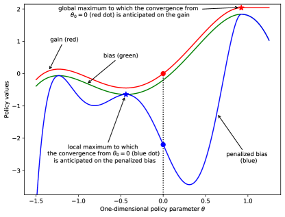
Figure 3: An illustration of a deep valley on the penalized bias landscape along with comparisons to gain and bias landscapes. The initial $\theta_{0}$ is at 0.

Second, the barrier function (23) contains only the gain value. In contrast, a penalty function likely involves the gain gradients, such as $\|\nabla g(\boldsymbol{\theta})\|$ in (27). This implies that first-order optimization on the penalized objective necessitates the second derivative (as in $\nabla\mathfrak{b}(\boldsymbol{\theta})=\nabla b(\boldsymbol{\theta})-\phi\nabla^{\intercal}g(\boldsymbol{\theta})\nabla^{2}g(\boldsymbol{\theta})$), whereas any second-order optimization necessitates the third derivative. Since a penalty method does not necessarily begin at a feasible point, its penalized objective, e.g. (27), cannot be turned into a function of solely gain terms similar to (23).

Third, we observe that the gain landscape (on which the barrier method’s preliminary operates) is more favourable than the penalized bias landscape in achieving higher local maxima. The penalized objective $\mathfrak{b}$ in (27) may create a deep valley in between its two local maxima, as illustrated in Fig 3. Thus, optimization from some initial point $\boldsymbol{\theta}_{0}$ in the valley is attracted to the nearest (instead of highest) local maximum of $\mathfrak{b}$. This phenomenon does not occur in the gain landscape when the gain optimization (part of the preliminary phase of the barrier method) is started at the same initial point $\boldsymbol{\theta}_{0}$. Note that such a valley of $\mathfrak{b}$ is formed partly because $\|\nabla g(\boldsymbol{\theta})\|_{2}^{2}$ is always zero at the stationary points of bias, but is likely to be non-zero otherwise.

6 Experimental setup

In this section, we discuss the implementation and experimental details for the proposed nBw-optimal policy gradient algorithm (Sec 5). We begin with environment descriptions (Sec 6.1), followed by policy parameterization (Sec 6.2) and the parameter values of Algo 1 and 2 (Sec 6.3). In Sec 6.4, we provide the settings for the discounted-reward policy gradient method, which is used for comparison. Throughout the experiments, $\log$ refers to the natural logarithm, i.e. $\log_{e}$. The research code is publicly available at https://github.com/tttor/nbwpg.

6.1 Environments

There are two types of environments that we consider in this work: a) environments for which all stationary policies are gain optimal, and b) those for which some stationary policies are gain optimal and some are not. Each environment type has three instances. The first type has Env-A1, Env-A2, and Env-A3, whereas the second type has Env-B1, Env-B2, and Env-B3. Both types share three common properties: i) all stationary policies induce unichain Markov chains, ii) the nBw optimality is the most selective, and iii) there is no terminal state, hence all environments are continuing (non-episodic).

In every environment, all states have the same number of available actions. That is, two actions per state. At some states, those two actions are duplicates (having the same transition probability and reward). This is simply to ease the implementation of policy parameterization, which accomodates generalization across 2-action states. Additionally, every environment’s initial state distribution $\mathring{p}$ has a single state support $s^{0}\in\mathcal{S}$, that is $\mathring{p}(s^{0})=1$.

The symbolic diagrams and descriptions for Env-A1, A2, B1, B2, and B3 are provided in Figs 4 and 5. Env-A3 is complex and unintuitive to draw therefore we describe it in words below.

Env-A3:

This environment has 4 states with 2 actions per state, yielding $16(=2^{4})$ stationary deterministic policies. It resembles $2$-by-$2$ grid-world navigation, whose start state $s^{0}$ is at the bottom-left, whereas goal state $s^{3}$ at the top-right. Each state has its own unique action set, namely: $s^{0}$ has East and North actions, $s^{1}$ (bottom-right) has West and North actions, $s^{2}$ (top-left) has East and South actions, and $s^{3}$ has 2 self-loop (self-transition) actions. In all but the goal state, the navigating agent goes to the intended direction at $90\%$ of the times. Otherwise, it goes to the other direction. Every action incurs a cost of $-1$, except those at the goal state (having a zero cost).

All stationary deterministic policies for this environment have an equal gain of $0$, hence all are gain optimal. There are 6 distinct bias values, ranging from $-17.000$ to $0.778$. There exist 4 nBw-optimal policies (out of 16, hence $4/16=0.25$) that choose any action at the start state $s^{0}$, East action at the top-left state $s^{2}$, North action at the bottom-right state $s^{1}$, and any action at the goal state $s^{3}$.

(a) Env-A1. There exist four stationary deterministic policies, whose gains are all $-1$. Two policies have the bias of $11$, whereas the other two have the bias of $12$. There are two nBw-optimal policies (out of four, hence $2/4=0.5$) that choose $a^{00}$ at $s^{0}$, and any action at $s^{1}$.

(b) Env-A2. There are 5 states (where $s^{4}$ is absorbing) and 2 actions per state, yielding $32(=2^{5})$ stationary deterministic policies. All of those policies have the same gain of 0, hence they are all gain optimal. There are 4 distinct bias values, namely $2$, $3$, $5$ and $6$. There exist 8 nBw-optimal policies (out of 32, hence $8/32=0.250$) that choose $a^{01}$ at $s^{0}$, $a^{30}$ at $s^{3}$, and any action at the other states.

(c) Env-B1. There are four stationary deterministic policies, from which there are 3 distinct gain values (i.e. $0.67,1.33,4$), and 4 distinct bias values (i.e. $-3,-1,0.22,1.11$). There exists a single nBw-optimal policy (out of four, hence $1/4=0.250$) that chooses $a^{01}$ at $s^{0}$, and $a^{11}$ at $s^{1}$. Its bias is of $-1$.

(d) Env-B2. The Taxi loop at $s^{2}$ refers to the 3-state Taxicab environment of hordijk_1985_disc, where $s^{2}$ denotes the state number 1 in the original environment description. The Taxi loop (including $s^{2}$) forms a recurrent class. Thus, this environment has 5 states in total, and 2 actions per state, yielding $32(=2^{5})$ stationary deterministic policies. There are 8 distinct gain values, ranging from $8.621$ to $13.345$, and 16 distinct bias values, ranging from $-1.683$ to $35.907$. There are 4 policies with the maximum gain, whose bias are of $-0.289$ and $16.367$. There exist 2 nBw-optimal policies (out of 32, hence $2/32=0.0625$) that choose $a^{00}$ at $s^{0}$, any action at $s^{1}$, and action number 2 (of the original description) at all states in the Taxi loop.

Figure 4: Symbolic diagrams of Env-A1, A2, B1, and B2. Each node indicates a state, which is labeled with a superscript state-index, i.e. $\mathcal{S}=\{s^{0},s^{1},\ldots,s^{|\mathcal{S}|-1}\}$. Each 3-tuple label of solid edges indicates the corresponding action $a$, immediate reward $r(s,a,s^{\prime})$, and transition probability $p(s^{\prime}|s,a)$. The action is labeled with 2-digit superscript action-index: the first digit denotes the state index in which such an action is available, whereas the second the action number (either $0$ or $1$) in that state. Here, all above-mentioned bias values are measured from a deterministic initial state $s_{0}=s^{0}$. For Env-A3 and B3, refer to the text in Sec 6.1 and Fig 5, respectively.

Figure 5: Env-B3. The Chain loop at $s^{2}$ refers to the 5-state Chain environment of strens_2000_bfrl, where $s^{2}$ denotes the state number 1 in the original environment description. The Chain loop (including $s^{2}$) forms a recurrent class. Thus, there are 7 states in total and 2 actions per state, yielding $128(=2^{7})$ stationary deterministic policies that induce 32 distinct gain values, ranging from $0.732$ to $3.677$, and 128 distinct bias values, ranging from $-14.461$ to $15.871$. There are 4 policies with the maximum gain, whose bias are of $-14.461,-7.461,-9.461$, and $-2.461$. There exists a single nBw-optimal policy (out of 128, hence $1/128\approx 0.008$) that chooses $a^{01}$ at $s^{0}$, $a^{10}$ at $s^{1}$, and forward actions at all states in the Chain loop. For more description, refer to the caption of Fig 4.

6.2 Policy parameterization

In order to visualize the parameter space in 2D plane, we limit the number of policy parameters to two. That is, $\boldsymbol{\theta}\in\Theta=\real{2}$, where $\boldsymbol{\theta}=[\theta_{0},\theta_{1}]^{\intercal}$. It turns out that this parameterization contains randomized stationary policies that are very close to the nBw-optimal policy for our target environments (Sec 6.1).

Thus, a randomized stationary policy $\pi\in\Pi_{\mathrm{S}}$ is parameterized as

$$\pi(a^{s0}|s;\boldsymbol{\theta})=\sigma(f(s)\theta_{0}+\theta_{1}),\quad\text{and}\quad\pi(a^{s1}|s;\boldsymbol{\theta})=1-\pi(a^{s0}|s;\boldsymbol{\theta}),\quad\forall s\in\mathcal{S},\forall\boldsymbol{\theta}\in\Theta,$$

where

• $a^{s0}$ and $a^{s1}$ are all two actions available at state $s$,

• $\sigma(x)=1/(1+\exp(-x))$ is the sigmoid function for an input $x$, and

• $f(s)\in\{0,1,\ldots,|\mathcal{S}|-1\}$ is the state feature function that returns the state index of $s$.

Note that such sigmoid parameterization does not contain stationary policies that are exactly deterministic (non-randomized), but contains those very close to being deterministic.

6.3 Algorithm parameters

Below, we list the default parameter values and settings of Algo 1 and 2.

• The policy parameterization is described in Sec 6.2. There are $1681(=41^{2})$ combination of $\theta_{0}$ and $\theta_{1}$ used as initial policy parameter values. They come from a discretized version of the parameter space $\Theta$ in the range of $-10$ to $+10$ with $0.5$ resolution in each dimension.

• The tolerance for gain-optimization convergence is $\epsilon\leftarrow 10^{-4}$. The $\ell_{2}$-norm is used.

• The initial barrier parameter is $\beta_{0}\leftarrow 0.1$ for Env-A, whereas $\beta_{0}\leftarrow 100$ for Env-B. This is based on tuning experiments described in Sec 7.4. The barrier divisor is always $\beta_{\mathrm{div}}\leftarrow 10$.

• The maximum inner and outer iterations are $n_{j}\leftarrow 100$ and $n_{k}\leftarrow 1$, respectively.

• The sample size is $n_{\mathrm{xep}}\leftarrow 16$, which is used in sampling-based approximation.

• The maximum timestep of an experiment-episode (trial) is set as $\hat{t}_{\mathrm{max}}^{\mathrm{xep}}\leftarrow t_{\mathrm{mix}}+5$, where $t_{\mathrm{mix}}\coloneqq\max_{\boldsymbol{\theta}\in\tilde{\Theta}}t_{\mathrm{mix}}^{\pi(\boldsymbol{\theta})}$. Here, $\tilde{\Theta}$ is a discretized version of $\Theta$ with $0.1$ resolution in the range of $-10$ to $+10$, and $5$ additional timesteps are to partially accomodate the mixing times of policies whose parameters are not contained in $\tilde{\Theta}$. Each $t_{\mathrm{mix}}^{\pi}$ is set to the smallest timestep $t$ when the entry-wise numerical difference between the transient and stationary state distributions satisfies $|p_{\pi}^{\star}(s)-p_{\pi}^{t}(s|s_{0})|\leq\mathrm{tol}_{abs}+\mathrm{tol}_{rel}\times p_{\pi}^{t}(s|s_{0})$ for a deterministic initial state $s_{0}$ and all states $s\in\mathcal{S}$, where $\mathrm{tol}_{abs}=10^{-6}$ and $\mathrm{tol}_{rel}=10^{-5}$.

• All policy evaluations are exact, hence exact state values $v$ and exact state-action values $q$. This can be thought of as having an oracle value function approximator. We remark that a naive estimator for $q_{b}^{\pi}(s,a)$ in (5) would be a total sum of rewards earned since the action $a$ is executed at state $s$, substracted by the last reward (approximating the gain) times the number of timesteps taken while following on a policy $\pi$ till the end of an experiment-episode.

• All step lengths are computed using the backtracking linesearch method (boyd_2004_cvxopt, Algo 9.2) with an initial step length of $1$ and a maximum of $100$ iterations.

• The gain optimization is carried out exactly since we focus on bias-only and bias-barrier optimization. This is to suppress the number of approximation layers, as well as to isolate the cause of improvement to solely the proposed expressions of the bias gradient (4), the bias Fisher (19), and the bias barrier (23). Note that the gain policy gradient is given by

  $$\nabla v_{g}(\boldsymbol{\theta})=\sum_{s\in\mathcal{S}}\sum_{a\in\mathcal{A}}p_{\pi}^{\star}(s)\ \pi(a|s;\boldsymbol{\theta})q_{b}^{\pi}(s,a)\nabla\log\pi(a|s;\boldsymbol{\theta}),\qquad\forall\boldsymbol{\theta}\in\Theta,$$ (28)

  as shown by sutton_2000_pgfnapprox.

6.4 Discounted-reward policy gradient methods

Here, we provide the setup for the discounted-reward policy gradient experiments, to which we compare our proposed nBw-optimal policy gradient method (Sec 5). Such a comparison is carried out because the nBw-optimal policies are also attainable via discounted settings whenever the discount factor is proper, as discussed in Sec 8. We begin with a brief overview of the discounted method.

The expected total discounted reward with a discount factor $\gamma\in[0,1)$ is defined as

$$v_{\gamma}(\pi,s)\coloneqq\lim_{t_{\mathrm{max}}\to\infty}\mathbb{E}_{A_{t}\sim\pi(\cdot|s_{t}),S_{t}\sim p(\cdot|s_{t},a_{t})}\mathopen{}\mathclose{{}\left[\sum_{t=0}^{t_{\mathrm{max}}-1}\gamma^{t}r(S_{t},A_{t})\Big{|}S_{0}=s,\pi}\right],\quad\forall s\in\mathcal{S},\forall\pi\in\Pi_{\mathrm{S}}.$$ (29)

Stacking $v_{\gamma}$ of all states $s\in\mathcal{S}$ gives us a vector $\boldsymbol{v}_{\gamma}(\pi)\in\real{|\mathcal{S}|}$. Thus, we can write

$$\boldsymbol{v}_{\gamma}(\pi)=\boldsymbol{P}_{\!\!\pi}^{\gamma}\boldsymbol{r}_{\!\!\pi},\quad\text{where}\ \boldsymbol{P}_{\!\!\pi}^{\gamma}\coloneqq\underbrace{\lim_{t_{\mathrm{max}}\to\infty}\sum_{t=0}^{t_{\mathrm{max}}-1}(\gamma\boldsymbol{P}_{\!\!\pi})^{t}=(\boldsymbol{I}-\gamma\boldsymbol{P}_{\!\!\pi})^{-1}}_{\text{See \cite[citet]{\@@bibref{Authors Phrase1YearPhrase2}{puterman_1994_mdp}{\@@citephrase{(}}{\@@citephrase{, Corollary~{}C.4)}}}}},\ \text{and}\ \boldsymbol{r}_{\!\!\pi}\in\real{|\mathcal{S}|}.$$ (30)

Each $[s_{0},s]$-component of $\boldsymbol{P}_{\!\!\pi}^{\gamma}\in\real{\mathcal{S}\times\mathcal{S}}$ indicates the improper discounted state probability. That is,

$$p_{\pi}^{\gamma}(s|s_{0})\coloneqq\lim_{t_{\mathrm{max}}\to\infty}\sum_{t=0}^{t_{\mathrm{max}}-1}\gamma^{t}\underbrace{\mathrm{Pr}\{S_{t}=s|s_{0},\pi\}}_{p_{\pi}^{t}(s|s_{0})},\ \text{which is improper as}\ \sum_{s\in\mathcal{S}}p_{\pi}^{\gamma}(s|s_{0})=\frac{1}{1-\gamma}\neq 1.$$

A policy $\pi_{\gamma}^{*}\in\Pi_{\mathrm{S}}$ is $\gamma$-discounted optimal if it satisfies $v_{\gamma}(\pi_{\gamma}^{*},s_{0})\geq v_{\gamma}(\pi,s_{0}),\forall\pi\in\Pi_{\mathrm{S}},\forall s_{0}\in\mathcal{S}$. As an approximation to this condition (involving partial ordering in all states $s_{0}\in\mathcal{S}$), a discounted-reward policy gradient method maximizes the discounted value of a policy with respect to some initial state distribution $\mathring{p}$, namely $\hat{\pi}_{\gamma}^{*}\in\operatorname*{\arg\!\max}_{\pi\in\Pi_{\mathrm{S}}}\mathbb{E}_{\mathring{p}}\mathopen{}\mathclose{{}\left[v_{\gamma}(\pi,S_{0})}\right]$. Since such an objective depends on $\mathring{p}$, the resulting optimal policy is said to be non-uniformly optimal (altman_1999_cmdp, Def 2.1).

In a similar fashion to (2), the policy parameter update needs a gradient of $v_{\gamma}$ along with its preconditioner, e.g. a Fisher matrix. sutton_2000_pgfnapprox showed that the gradient is given by

$$\nabla v_{\gamma}(\boldsymbol{\theta},s_{0}) =\sum_{s\in\mathcal{S}}p_{\pi}^{\gamma}(s|s_{0})\sum_{a\in\mathcal{A}}q_{\gamma}^{\pi}(s,a)\nabla\pi(a|s;\boldsymbol{\theta})$$

$$=\sum_{t=0}^{\infty}\sum_{s\in\mathcal{S}}p_{\pi}^{t}(s|s_{0})\bigg{[}\gamma^{t}\underbrace{\sum_{a\in\mathcal{A}}q_{\gamma}^{\pi}(s,a)\nabla\pi(a|s;\boldsymbol{\theta})}_{\text{The so-called immediate gradient}}\bigg{]}$$ (31)

$$=\frac{1}{1-\gamma}\sum_{s\in\mathcal{S}}\underbrace{(1-\gamma)p_{\pi}^{\gamma}(s|s_{0})}_{\text{a proper probability}}\sum_{a\in\mathcal{A}}q_{\gamma}^{\pi}(s,a)\nabla\pi(a|s;\boldsymbol{\theta}),\qquad\forall\boldsymbol{\theta}\in\Theta,\forall s_{0}\in\mathcal{S},$$ (32)

where the last expresion enables approximation by sampling from the (proper, normalized) discounted state distribution, i.e. $(1-\gamma)p_{\pi}^{\gamma}(s|s_{0})$. Here, $q_{\gamma}^{\pi}$ denotes the discounted-reward state-action value. Furthermore, bagnell_2003_covps; peters_2003_rlhum introduced the following discounted-reward Fisher matrix (for preconditioning the gradient (32)), for all $\boldsymbol{\theta}\in\Theta$ and all $s_{0}\in\mathcal{S}$,

$$\boldsymbol{\Phi}_{\!\gamma a}(\boldsymbol{\theta},s_{0})\coloneqq\sum_{s\in\mathcal{S}}\underbrace{(1-\gamma)p_{\pi}^{\gamma}(s|s_{0})}_{\text{a proper probability}}\underbrace{\sum_{a\in\mathcal{A}}\pi(a|s;\boldsymbol{\theta})\nabla\log\pi(a|s;\boldsymbol{\theta})\nabla^{\intercal}\log\pi(a|s;\boldsymbol{\theta})}_{\text{The action Fisher $\boldsymbol{\Phi}_{\!a}(\boldsymbol{\theta},s)$ defined in \eqref{equ:fisher_gain}}},$$ (33)

which follows the same pattern as the gain and bias Fisher matrices (Sec 4). That is, the Fisher matrix of an optimality criterion is defined as the action Fisher (15) weighted by the corresponding state distribution. This can also be seen as following the pattern of policy value formulas, e.g. (30).

The normalization on $p_{\pi}^{\gamma}(s|s_{0})$ in (32, 33) implies that $\mathrm{Pr}\{S_{t}=s|s_{0},\pi\}$ is weighted by $(1-\gamma)\gamma^{t}$ at each timestep $t=0,1,\ldots$. This weight turns out to be equal to the probability that the Markov process terminates (“first success”) after $t+1$ timesteps (“trials”), yielding a sequence of $\ell=t+1$ states. This indeed follows a geometric distribution $Geo(p=1-\gamma)$ that gives

$$\mathrm{Pr}\{L=\ell\}=(1-p)^{\ell-1}p=(1-(1-\gamma))^{(t+1)-1}(1-\gamma)=\gamma^{t}(1-\gamma),\quad\text{for $\ell=1,2,\ldots$}.$$

To sample a single state from $(1-\gamma)p_{\pi}^{\gamma}$, one needs to sample a sequence length $\ell$ from $Geo(p=1-\gamma)$, then run the process under $\pi$ from $t=0$ to $\ell-1$. Finally, the state $S_{\ell}\sim p(\cdot|s_{\ell-1},a_{\ell-1})$ is the desired state sample (kumar_2020_zodpg, Algo 3). A more sample-efficient technique is proposed by thomas_2014_biasnac. It leverages the expression in (31) so that $\nabla v_{\gamma}$ is estimated using state samples $S_{t}\sim p_{\pi}^{t}$ drawn from undiscounted state distributions from $t=0$ till some finite timestep (truncating the infinite-horizon model). Note that in (31), $\gamma$ is used to discount the immediate gradient.

We consider discounting as an approximation technique towards maximizing the average reward (gain) objective, as in $\lim_{\gamma\to 1}(1-\gamma)v_{\gamma}(\pi)=v_{g}(\pi)$, see puterman_1994_mdp. This is suitable for environments without inherent notion of discounting. Therefore, the exact discounted reward experiments in this work maximize the scaled discounted value, i.e. $(1-\gamma)v_{\gamma}(\pi)$. The multiplication by $(1-\gamma)$ gives expressions that enable sampling for the gradients (32) and the Fisher matrix (33). The factor $(1-\gamma)$ also helps avoid numerical issues because of a very large range of $v_{\gamma}(\pi)$ across all policies $\pi$ (whenever $\gamma$ is very close to 1).

For the exact discounted reward experiments in Sec 7, we applied $\gamma$ values shown in Table 1.

Table 1: The discount factors $\gamma$ used in three scenarios of exact discounted reward experiments. Here, $\gamma_{\mathrm{Bw}}$ denotes the Blackwell’s discount factor as in (34). For environment descriptions, refer to Sec 6.1.

Scenarios	Environments
	A1	A2	A3	B1	B2	B3
$\gamma<\gamma_{\mathrm{Bw}}$	$0.50$	$0.20$	$0.00$	$0.00$	$0.30$	$0.50$
$\gamma\approx\gamma_{\mathrm{Bw}}$	$0.95$	$0.55$	$0.05$	$0.05$	$0.80$	$0.85$
$\gamma_{\mathrm{Bw}}<\gamma\approx 1$	$0.99999$

7 Experimental results

Our primary experimental aim is to validate and gain insights into the fundamental mechanisms of our algorithms, rather than demonstrating performance on a large RL problem. To this end, we consider a small but sufficient setup of benchmark environments and a policy parameterized as a single neuron with two weights, i.e. $\boldsymbol{\theta}=[\theta_{0},\theta_{1}]^{\intercal}\in\real{2}$, as described further in Sec 6. This allows us to visualize the algorithm performance across a large portion of the policy space via enumeration.

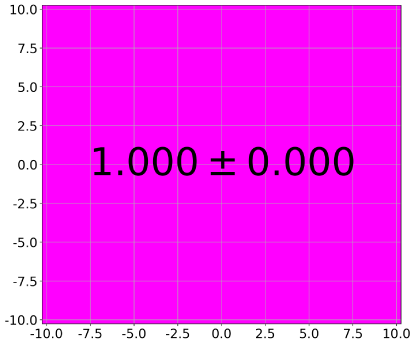
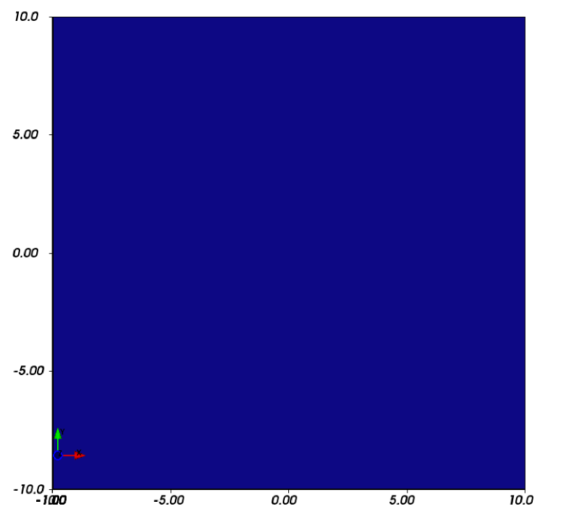
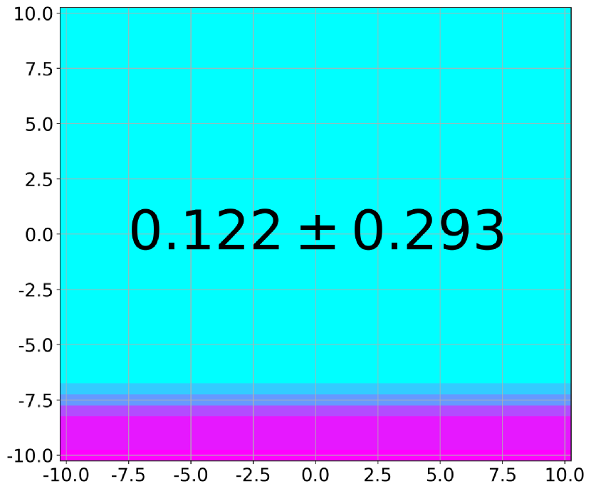
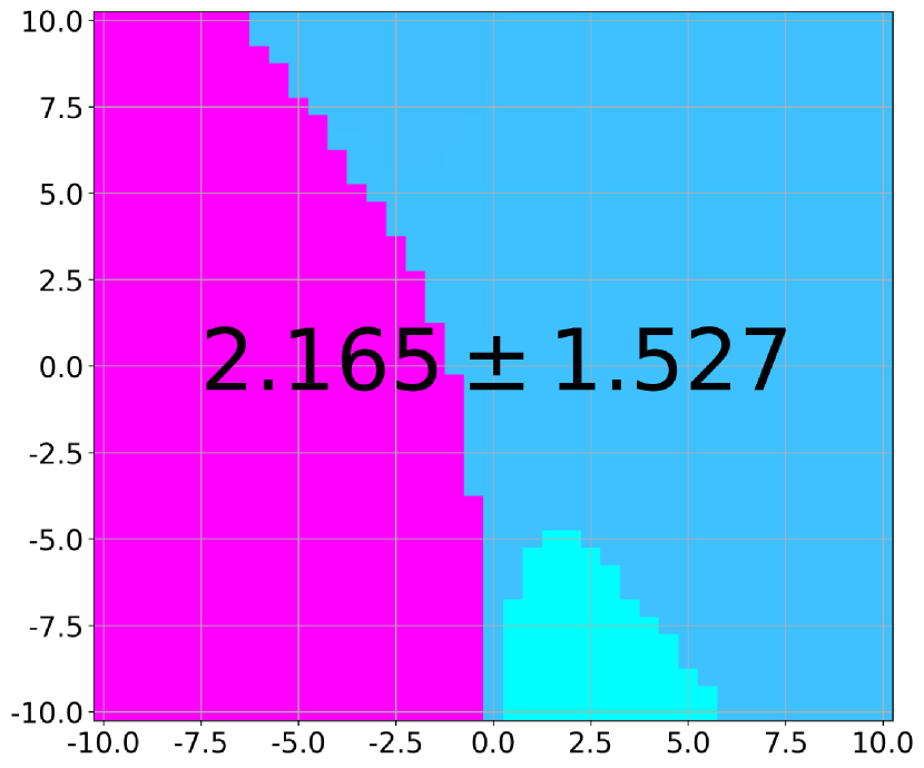
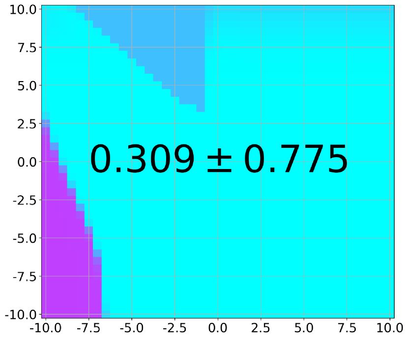
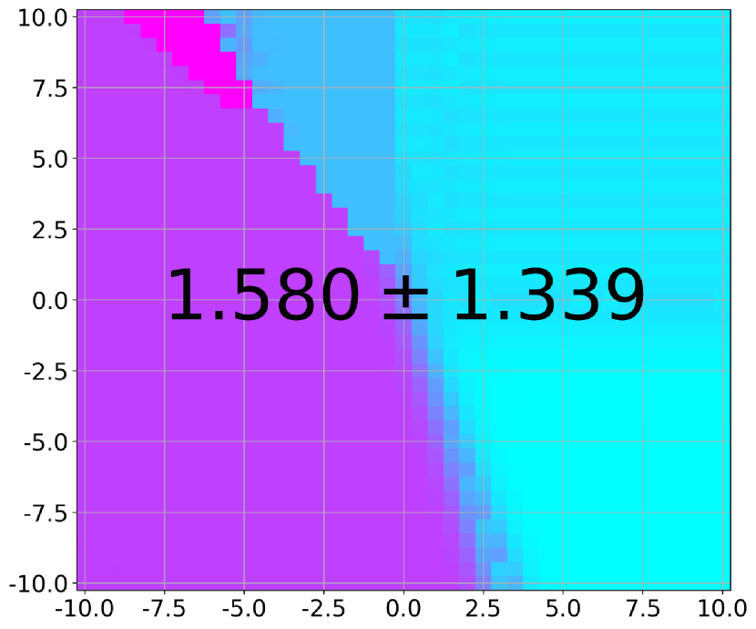
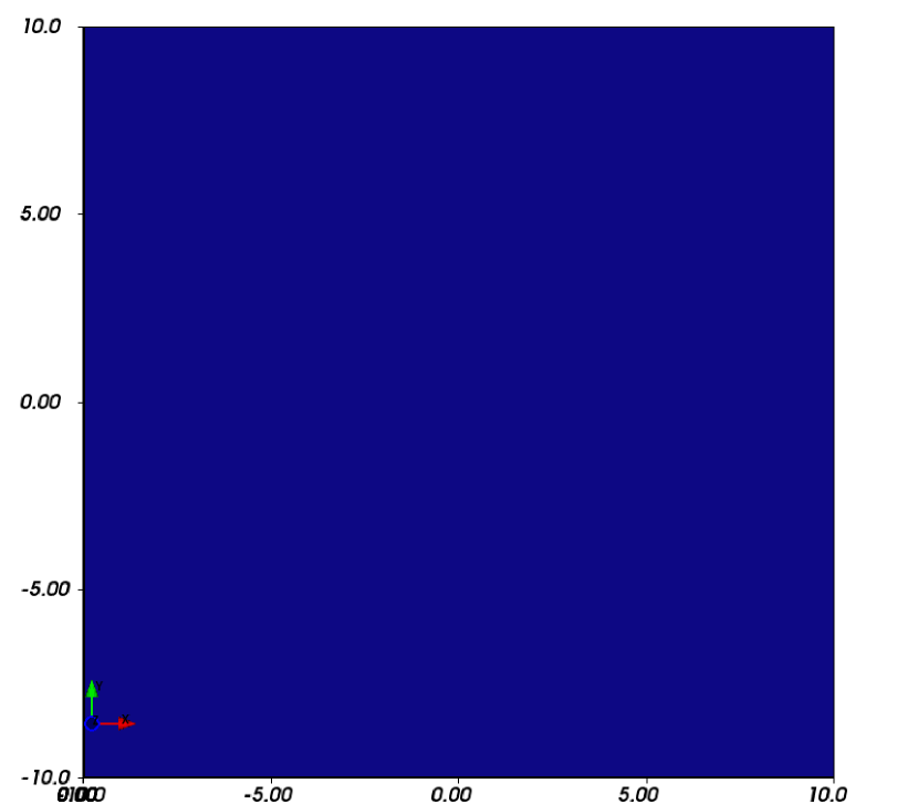
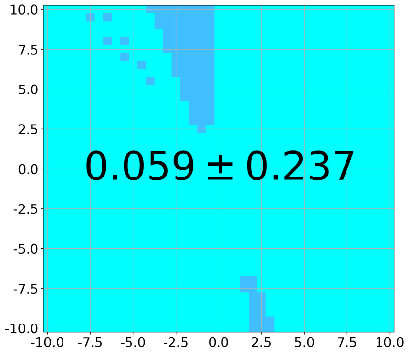
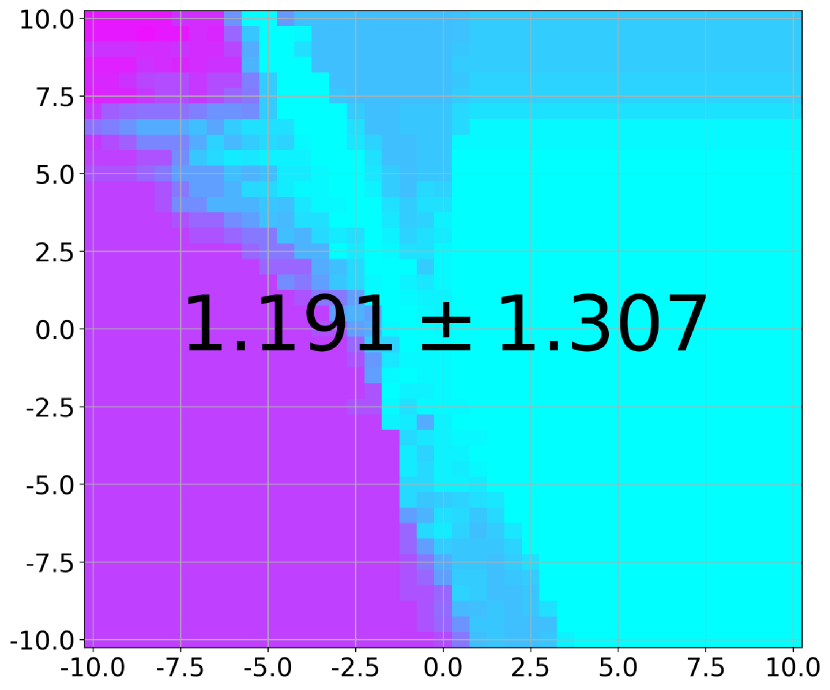
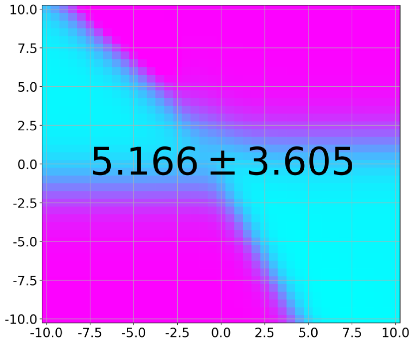
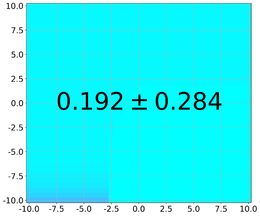
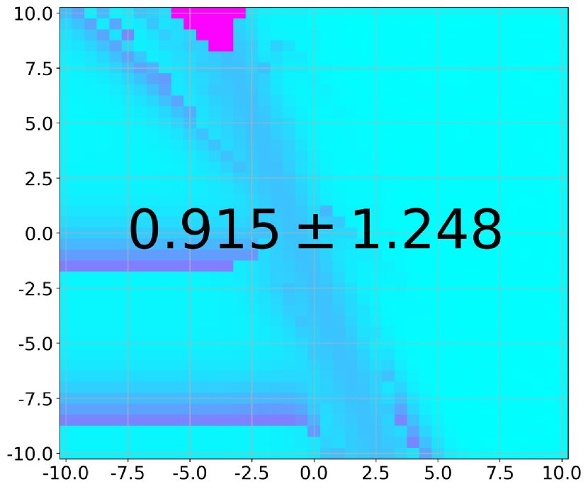
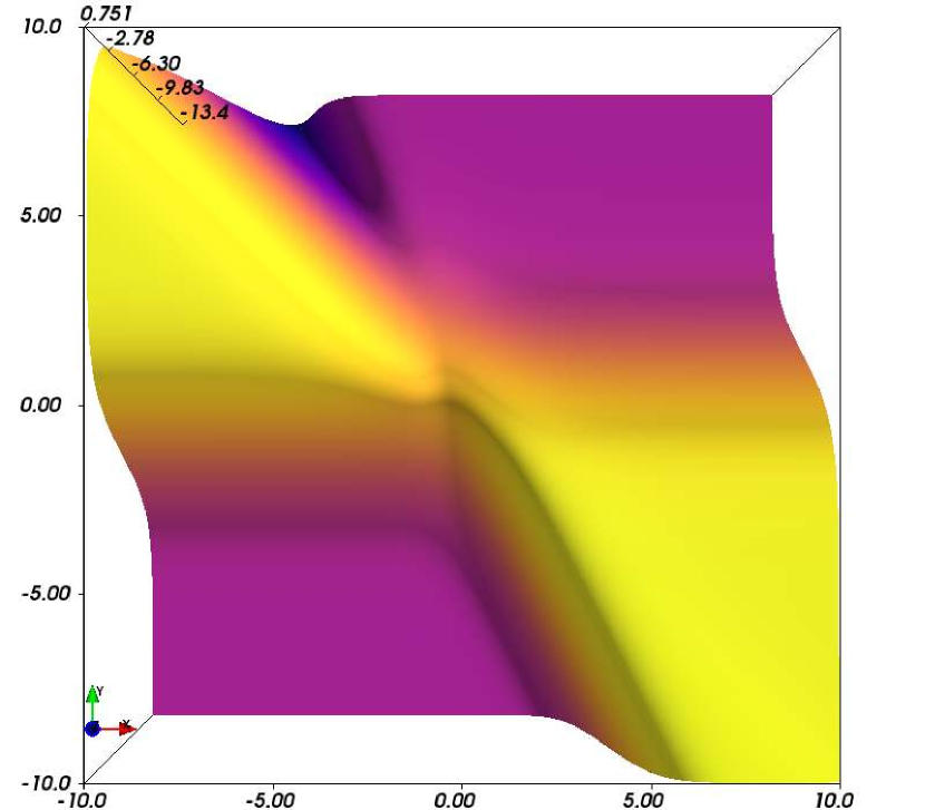
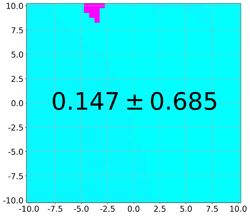
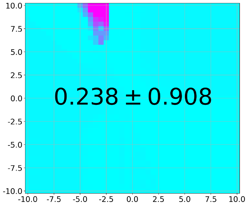
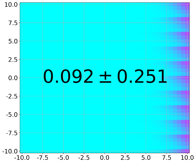
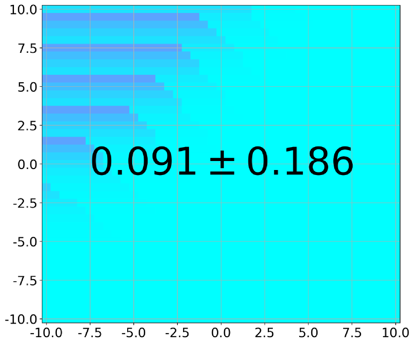
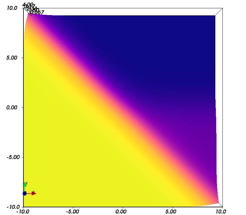
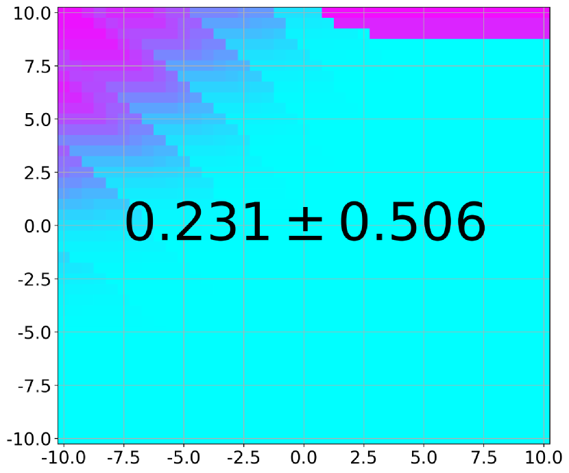
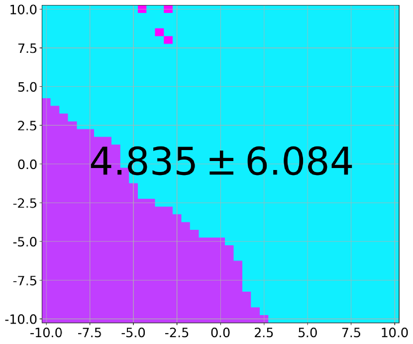
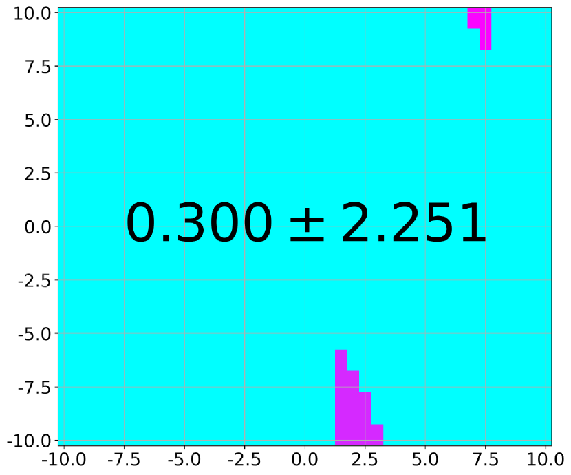
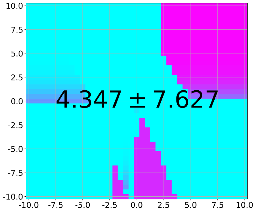
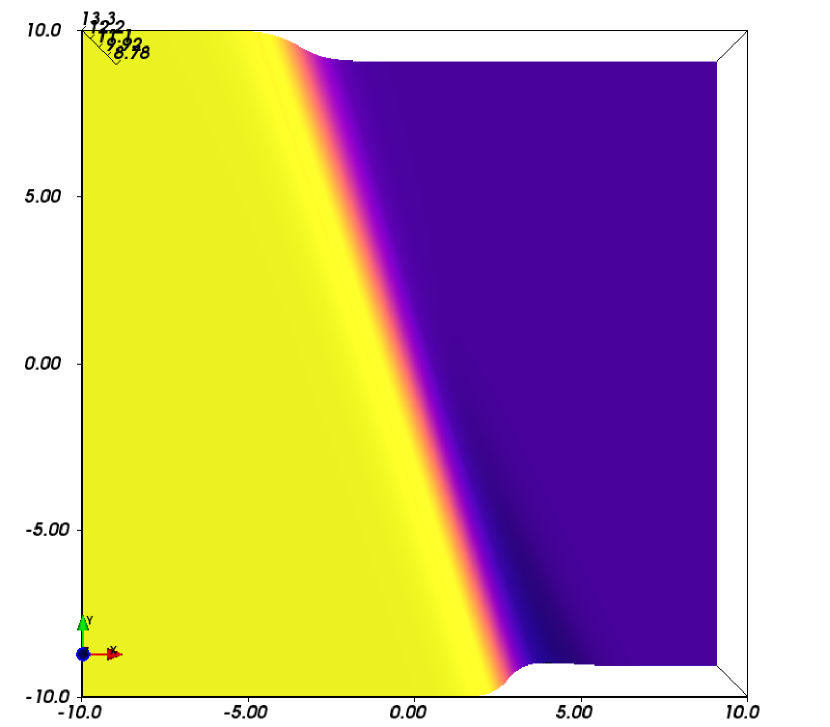
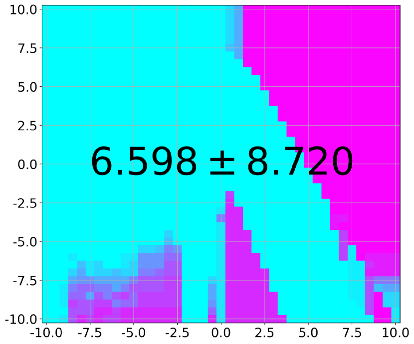
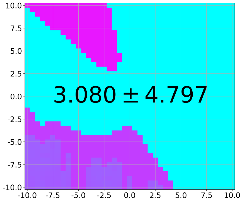
(a) $\gamma<\gamma_{\mathrm{Bw}}$

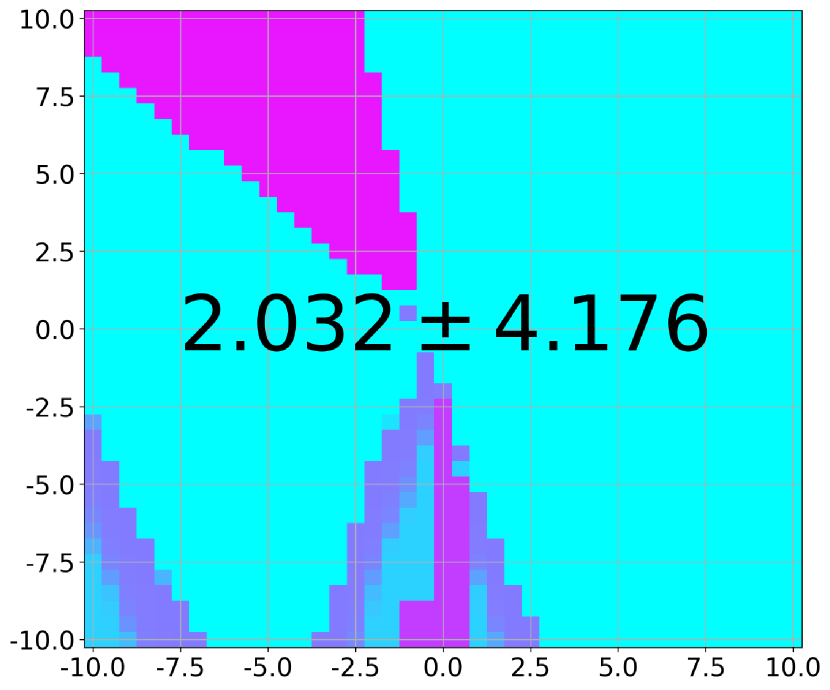
(b) $\gamma\approx\gamma_{\mathrm{Bw}}$

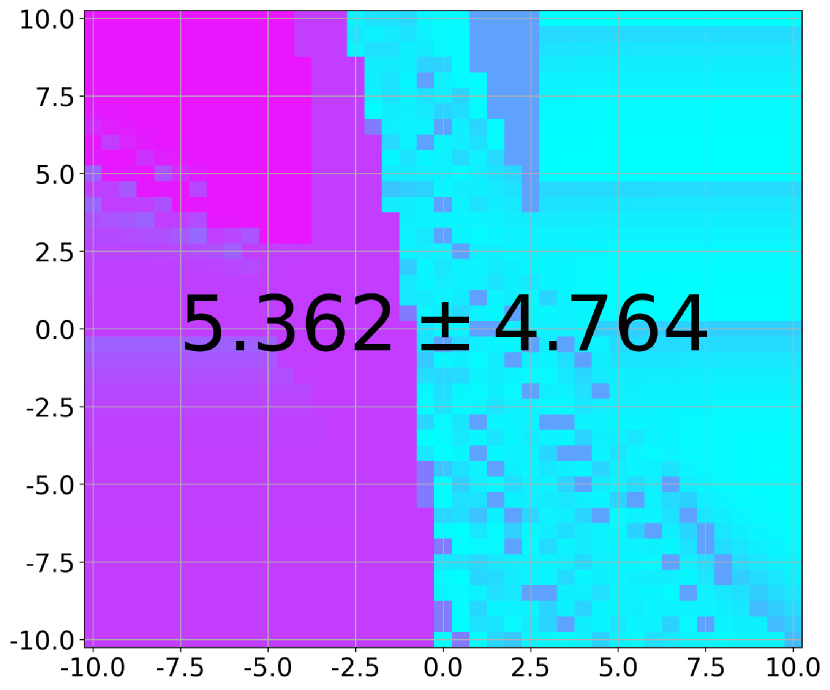
(c) $\gamma_{\mathrm{Bw}}<\gamma\approx 1$

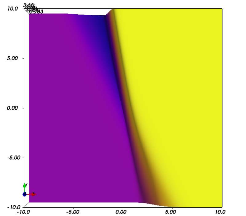
(d) Gain landscape

(e) Bias landscape

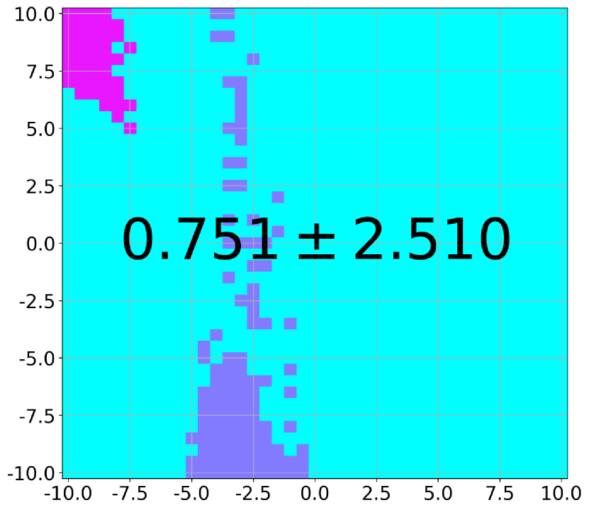
(f) Ours

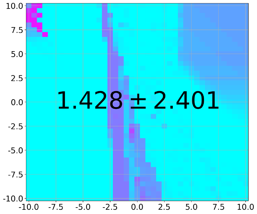
(g) Ours (sampling)

Figure 6: Evaluations of our Algo 1 with policy parameter $\boldsymbol{\theta}\in\real{2}$ (horizontal and vertical axes) on 6 environments (rows). The landscape plots map low:dark-blue and high:yellow. The other plots show the absolute difference or error (low:blue to high:magenta) between the bias of the nBw-optimal deterministic policy and of the resulting randomized policy, where the 2D-coordinate indicates the initial value of $\boldsymbol{\theta}$. The numbers in the middle indicate the mean and standard deviation across $41^{2}$ grid values. The lowest absolute bias difference (blue) is desirable. For experimental setup, see Sec 6.

7.1 Main experimental results

Fig 6 presents our main experimental results on six environments (Sec 6.1) as rows. The 4th and 5th columns depict optimization landscapes, where each 2D coordinate represents a randomized stationary policy whose gain and bias values are indicated by the coordinates’ colors. Here, the color-maps are normalized to the minimum-maximum range of the gain and bias of deterministic policies: the minimum is mapped to dark-blue and the maximum to yellow. Note that the gain landscape plots of Env-A1, A2, and A3 display only dark-blue colors because all stationary policies have the same gain value. On the other hand, the bias landscape of Env-B3 does not display the dark-blue and yellow colors because the displayed portion of the parameter space does not include randomized policies close enough to deterministic policies with minimum and maximum bias values.

The average-reward policy gradient method operates in the gain landscape (4th column); performing gain maximization. In the first top-3 environments (Env-A), it immediately reaches the global maxima region because all stationary policies are gain optimal. Therefore, it is imperative to employ our proposed method that switches to optimizing the bias-barrier (23) towards the highest bias (the yellow region in the 5th column), yielding nBw-optimal policies.

The situation for the bottom-3 environments (Env-B) is different in that some policies are gain optimal (the yellow region in the 4th column), some are not. In these environments, once the gain maximization is deemed converged (near or in the yellow region in the 4th column), the bias-barrier optimization (23) kicks in. The barrier component prevents the optimization iterates from going outside the gain optimal region (such iterates operate in the bias-barrier landscape, which looks like the bias landscape (5th column) in region where the policies are gain optimal). Thus, in the bottom-3 environments, the nBw-optimal policies are represented by the coordinates, whose colors are yellow (the highest) in the gain landscape and are violet (not the highest value) in the bias landscape. Note that by optimal policies, we mean approximately optimal policies since all policies represented in the plots are randomized (those approximately optimal are very close to being deterministic).

In what follows, we discuss comparisons between discounted-reward (1st, 2nd, 3rd columns) and our proposed (6th column) policy gradient methods in exact settings where there is no sampling-based approximation. Then, we discuss the behaviour of our proposed method in sampling experiments (7th right-most column), and compare it to its exact variant (6th column). Here, the performance of a method is indicated by the absolute error (difference) between the bias of the resulting randomized policy and of the nBw-optimal deterministic policy. The lowest error is mapped to blue, whereas the highest to magenta. These become the two extreme colors in the error plots in all but landscape columns in Fig 6. In those error plots, each 2D coordinate indicates the initial policy parameter, whereas the coordinate’s color indicates the bias error of a policy parameterized by the final policy parameter. Note that a high performance method has an error plot dominated by blue.

First, in exact settings, our proposed Algo 1 compares favourably with the discounted reward method whose performance is sensitive to the discount factor $\gamma\in[0,1)$. Our proposed algorithm is superior to those with poor choices of $\gamma$ (either too low or too high). It is better or at least on par with its discounted counterpart whose $\gamma$ is close to its critical value $\gamma_{\mathrm{Bw}}$, which is unknown in practice.

As can be observed from the 1st column, $\gamma<\gamma_{\mathrm{Bw}}$ generally results in suboptimal policies with respect to Blackwell optimality (Sec 8). This is indicated by larger magenta regions in the 1st than 2nd columns. Increasing $\gamma$ too close to 1 also results in larger magenta regions in the 3rd column, compared to the 2nd column (where $\gamma\approx\gamma_{\mathrm{Bw}}$). This is as anticipated since the scaled discounted reward is equal to the gain as $\gamma\to 1$. Hence, optimizing discounted rewards with such high $\gamma$ tends to behave like its average reward (gain) counterpart, which is undesirable for our six environments because gain optimality is underselective for the induced unichain MDPs.

The 2nd column represents a discounted reward variant with a proper $\gamma\approx\gamma_{\mathrm{Bw}}$, by which the nBw-optimal policy is also attainable (Sec 8). Therefore, its error plot is expected to be similar to that of our proposed method (6th column). Ours however is discounting-free so that it does not suffer from the performance sensitivity with respect to $\gamma$ values (as discussed in the previous paragraph). More importantly, its hyperparameter $\beta_{0}$ merely serves as the initial value for the barrier parameter $\beta$, which is then shrunk down to $0$ as the optimization iteration increases in Algo 1. This is in contrast to $\gamma$ that which is held fixed during optimization. In Sec 7.4, it is empirically shown that the performance is less sensitive to $\beta_{0}$ than to $\gamma$ (whose effects to performance are depicted in the 1st to 3rd columns).

Second, we compare the exact variant of Algo 1 (6th column) with its approximation (7th right-most column). Here, the approximation comes from sampling-based estimates of the gradients and Fisher matrices of the gain and bias-barrier functions, as prescribed by the sampling procedure in Algo 2. It can be seen that the sampling-based approximation results are reasonably close to the exact’s in most part of the policy parameter space. They are anticipated to follow the law of large numbers.

7.2 Decomposition of the bias gradients

We empirically investigate the contribution of each term of the bias gradient expression (4). Each term is computed exactly. The pre-mixing terms are gradually added up term-by-term from $t=0$ to $t_{\mathrm{mix}}^{\pi}-1$, then the single post-mixing term at $t_{\mathrm{mix}}^{\pi}$ is finally added up to the total of pre-mixing terms.

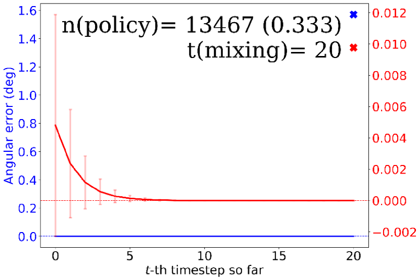
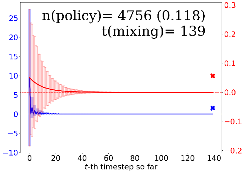
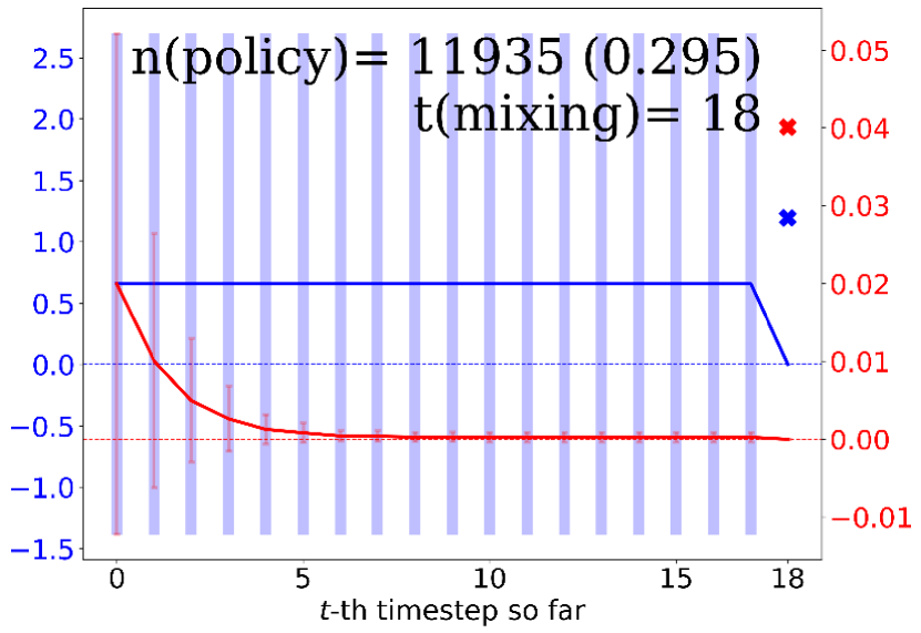
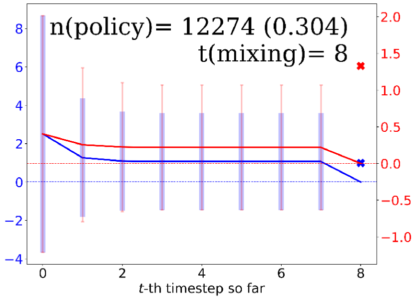
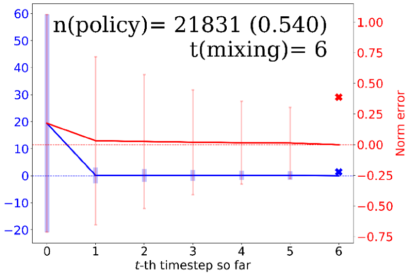
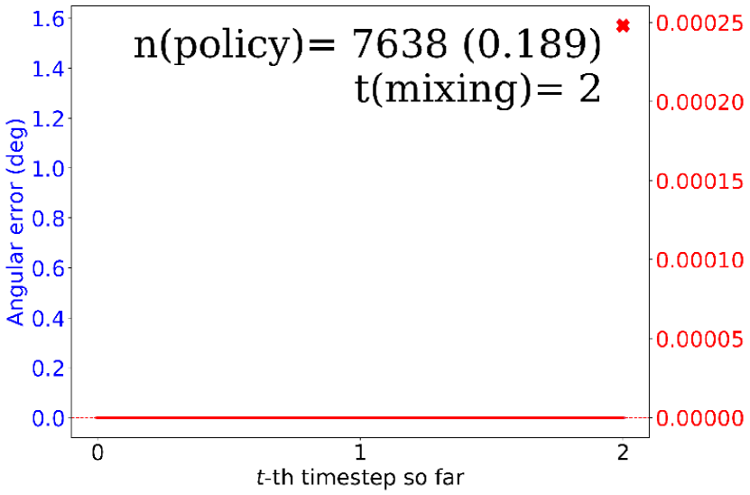
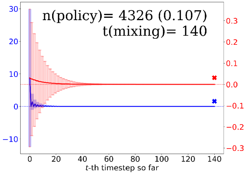
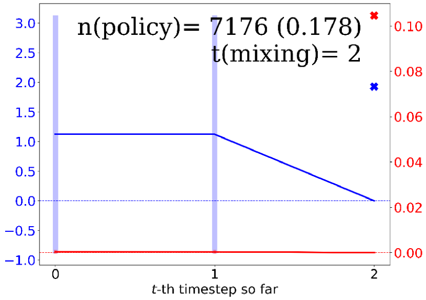
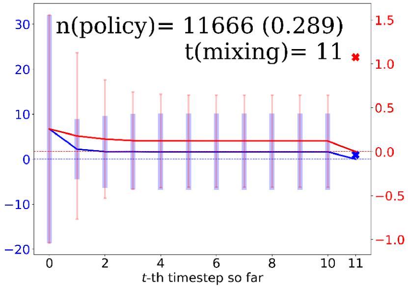
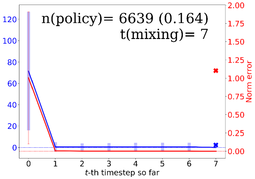
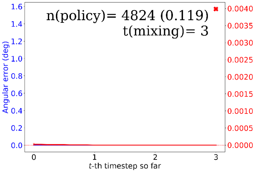
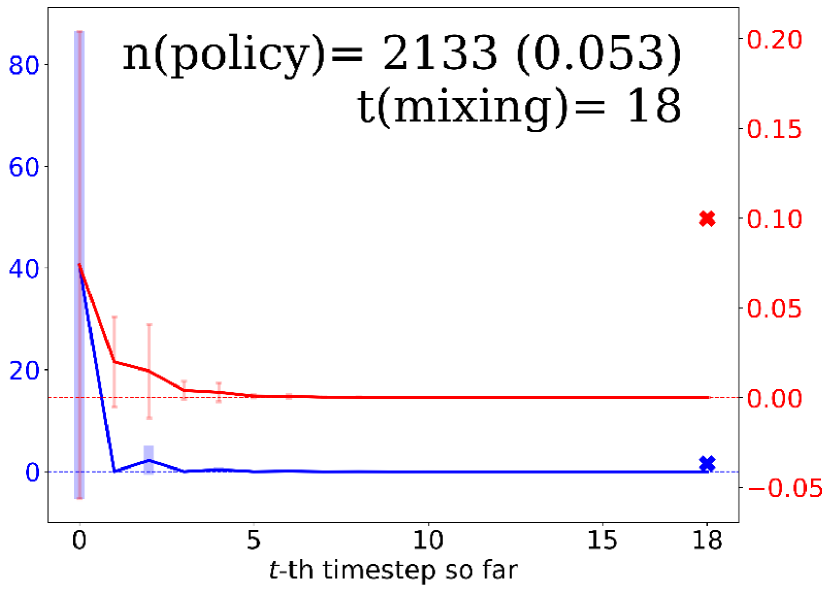
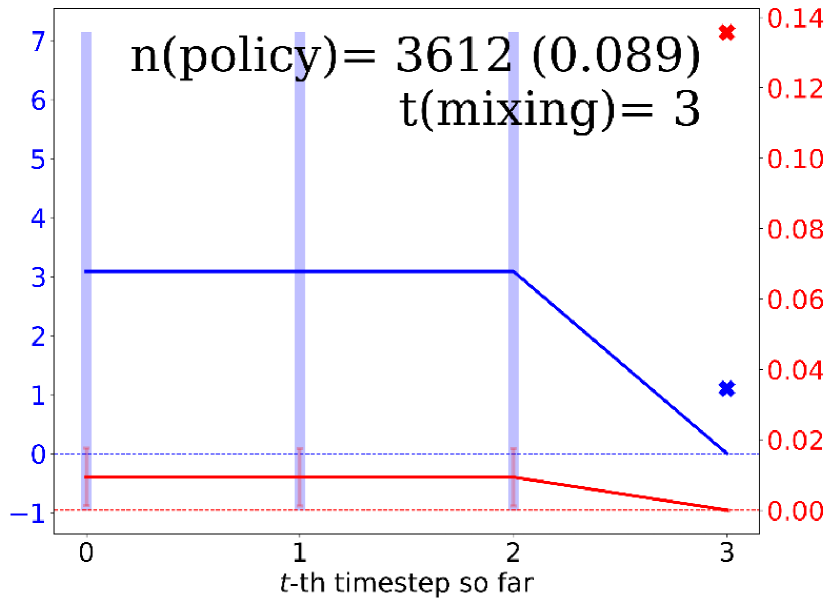
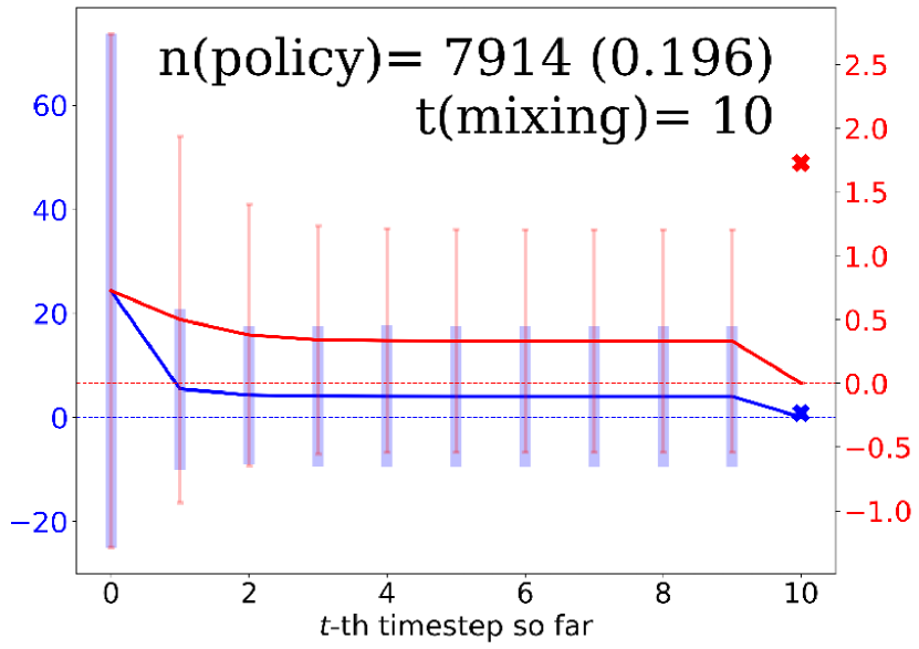
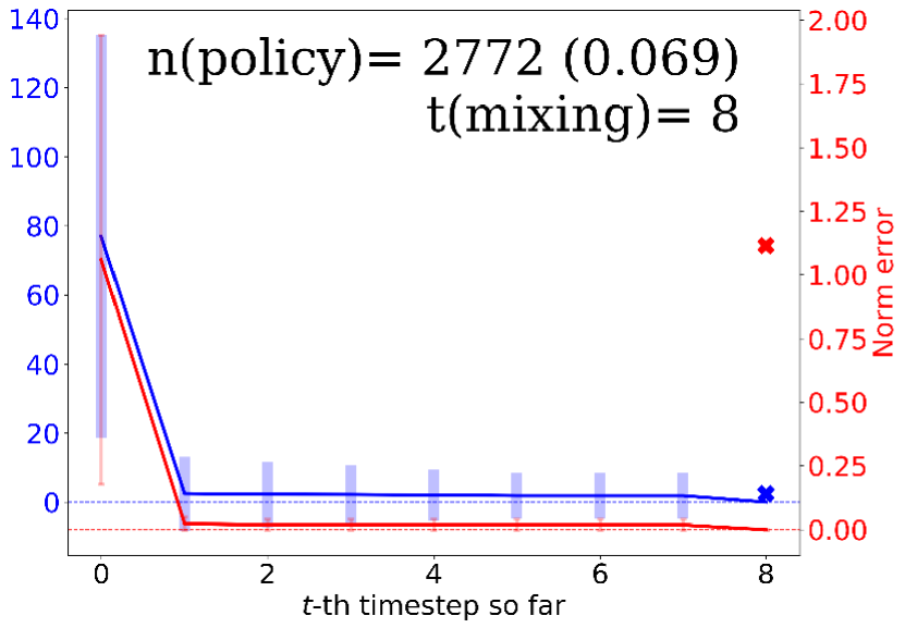
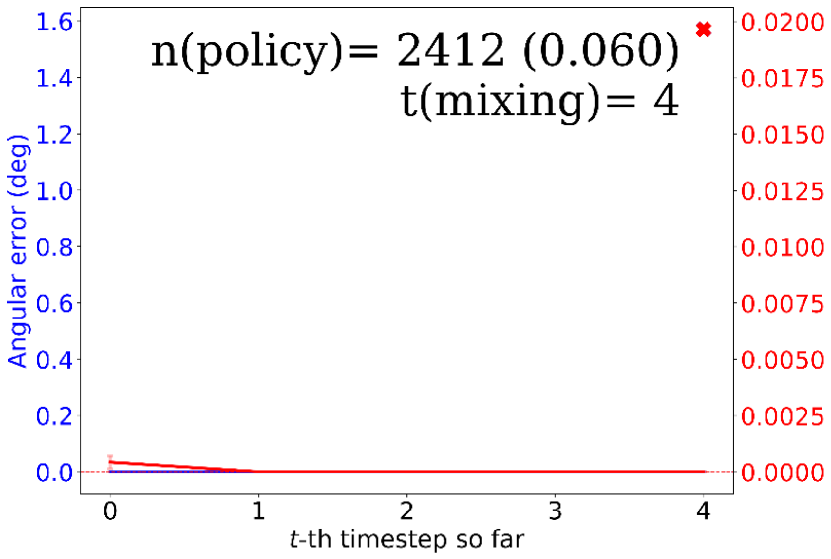
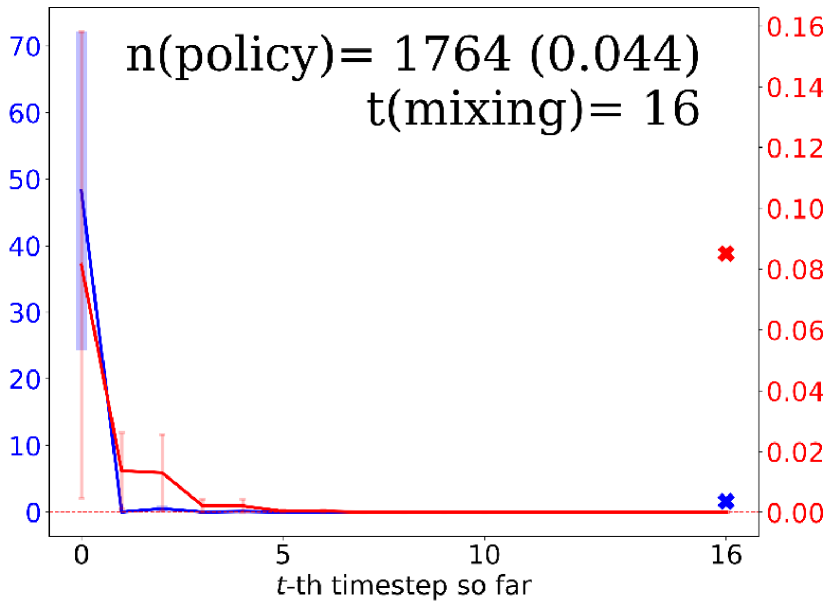
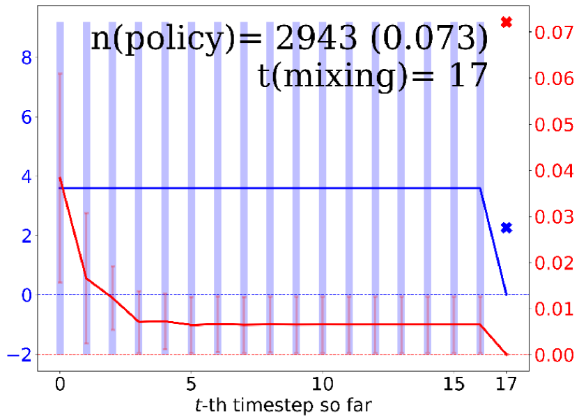
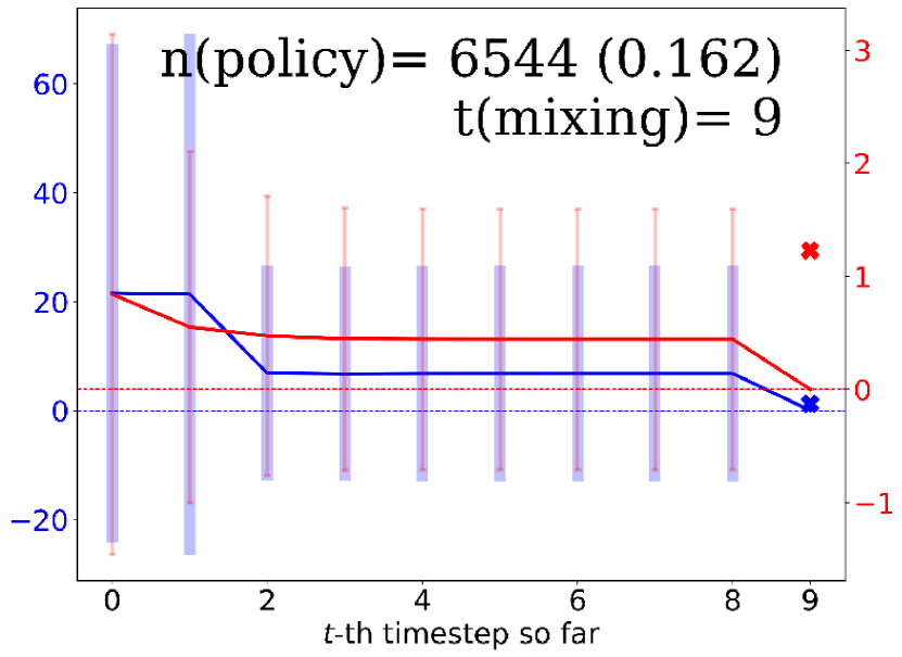
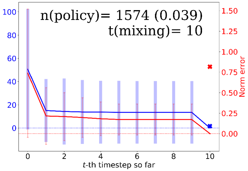
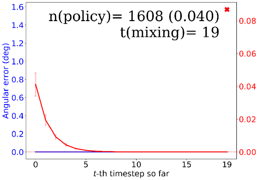
(a) Env-A1

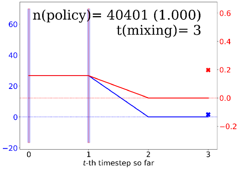
(b) Env-A2

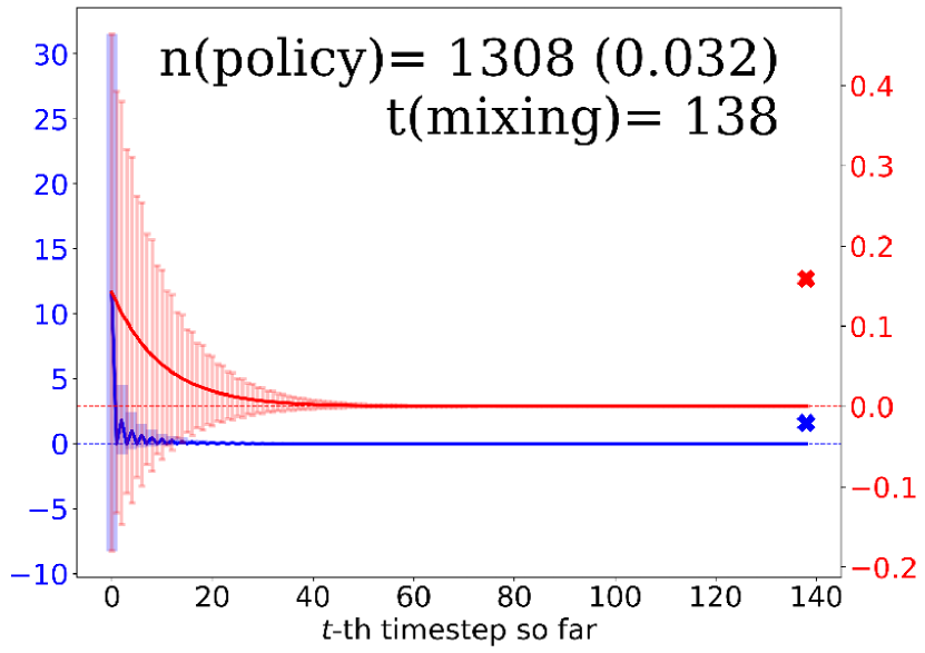
(c) Env-A3

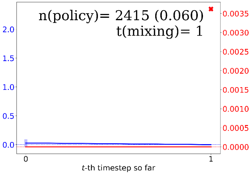
(d) Env-B1

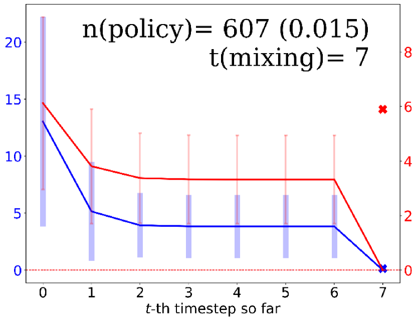
(e) Env-B2

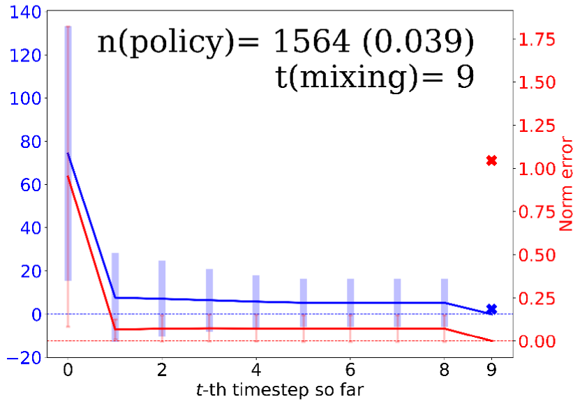
(f) Env-B3

Figure 7: The error of the exact gradual summation of bias gradient terms with respect to the exact full bias gradient (4). The blue line indicates the angular error, whereas the red the $\ell_{2}$-norm error. These bias gradients are of policies, whose mixing time is the most common (top row) in that it is induced by most policies (out of $40401$ policies in a $201$-by-$201$-grid policy parameter space from $-10$ to $+10$ with $0.1$ uniform spacing in each parameter dimension). Those of the 2nd, 3rd, up to 5th most common mixing times are in the 2nd, 3rd, down to the bottom-most row, respectively. The error bar indicates the standard deviation across the corresponding error values of those many policies. The blue and red crosses (on the right part of each subfigure) show the angular and norm errors of the single post-mixing term. In some subfigures, the blue cross coincides with the red one (note however, their vertical axes are different). For experimental setup, see Sec 6.

Fig 7 shows the error of the exact gradual summation with respect to the exact full gradients of the bias; hence, the error after all summations are carried out is exactly zero. There are direction (angular) and magnitude (norm) errors. Note that in practice, the magnitude error can be folded into (compensated by) the optimization step length (i.e. the learning rate).

One apparent trait is that the error drops always occur either in the beginning (the first few terms) of the summation, at the end, or both. Generally, there is little to no error change in between. This suggests at least two phenomenons. First, pre-mixing terms at later timesteps contribute less to the bias gradient, compared to the first few. Second, the single post-mixing term is likely to have a significant contribution to the bias gradient.

7.3 Bias-only optimization

In this section, we focus on bias-only optimization (cf. gain-then-bias-barrier optimization in Sec 5). For environments where all policies are gain optimal (i.e. Env-A1, A2, A3), bias-only optimization returns nBw-optimal policies. For others (i.e. Env-B1, B2, B3), it returns policies that have the maximum bias but not necessarily the maximum gain (thus, they are not necessarily nBw-optimal).

In exact settings, there are four schemes of bias-only optimization due to different preconditioning matrices $\boldsymbol{C}$ in (2). They are as follows.

1. Identity: $\boldsymbol{C}\leftarrow\boldsymbol{I}$ for an identity matrix $\boldsymbol{I}$. This yields standard (vanilla) gradients.

2. Hessian: $\boldsymbol{C}\leftarrow\nabla^{2}v_{b}(\boldsymbol{\theta})$, where the Hessian $\nabla^{2}v_{b}(\boldsymbol{\theta})$ is modified by adding $e\boldsymbol{I}$ for a small positive $e$ until it becomes a positive definite matrix (checked by the Cholesky test).

3. Analytic Fisher: $\boldsymbol{C}\leftarrow\boldsymbol{\Phi}_{\!ba}(\boldsymbol{\theta})$ from (18), yielding natural gradients. That the Fisher matrix is positive-semidefinite (instead of positive-definite) is a typical problem for optimization methods that involve the Fisher matrix inversion, such as (2). There are several resolutions to this, e.g. using the pseudo-inverse, or adding a small positive-definite term, say $10^{-3}\boldsymbol{I}$.

4. Sampling-enabler Fisher: $\boldsymbol{C}\leftarrow\tilde{\boldsymbol{\Phi}}_{\!ba}(\boldsymbol{\theta})$ from (19), yielding approximate natural gradients (which are approximations to those of Scheme iii. due some ignored terms, as described in Sec 4). Here, a sampling-enabler expression enables sampling because it contains only expectation terms. In exact settings, those expectations are computed exactly.

In sampling-based approximation settings, there are two schemes approximating Schemes i. and iv.. Here, approximation refers to estimating the gradient and Fisher of the bias by their sample means, as described in Algo 2. We did not perform approximation experiments corresponding to Schemes ii. and iii. because the Hessian $\nabla^{2}v_{b}$ (which is a straightforward differentiation of (3)) and the bias Fisher $\boldsymbol{\Phi}_{\!ba}$ (18) do not enable sampling-based approximation.

Fig 8 shows the experiment results of bias-only optimization. In exact settings, the natural gradients (both Schemes iii. and iv.) mostly yield higher bias than the standard gradients (Scheme i.), as anticipated in Sec 4. Interestingly, as a preconditioning matrix, the proposed Fisher often outperforms the modified Hessian (Scheme ii.), otherwise it is slightly worse. More importantly, the sampling-enabler Fisher (computed exactly) maintains this benefit.

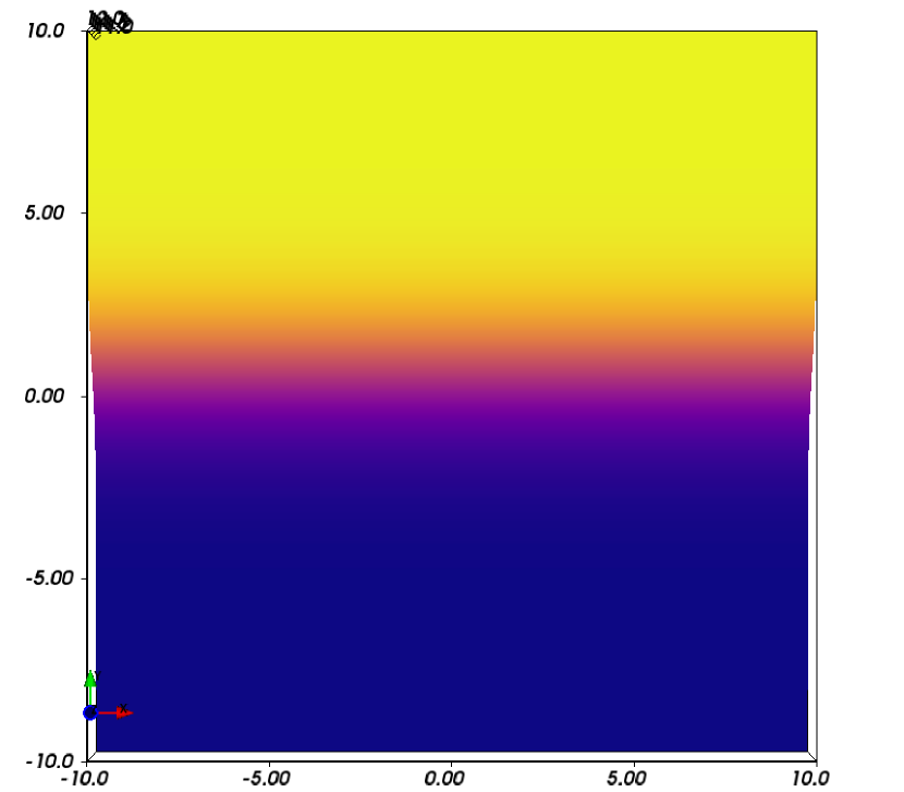
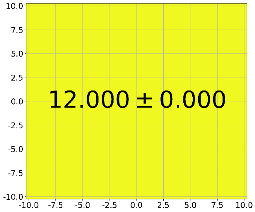
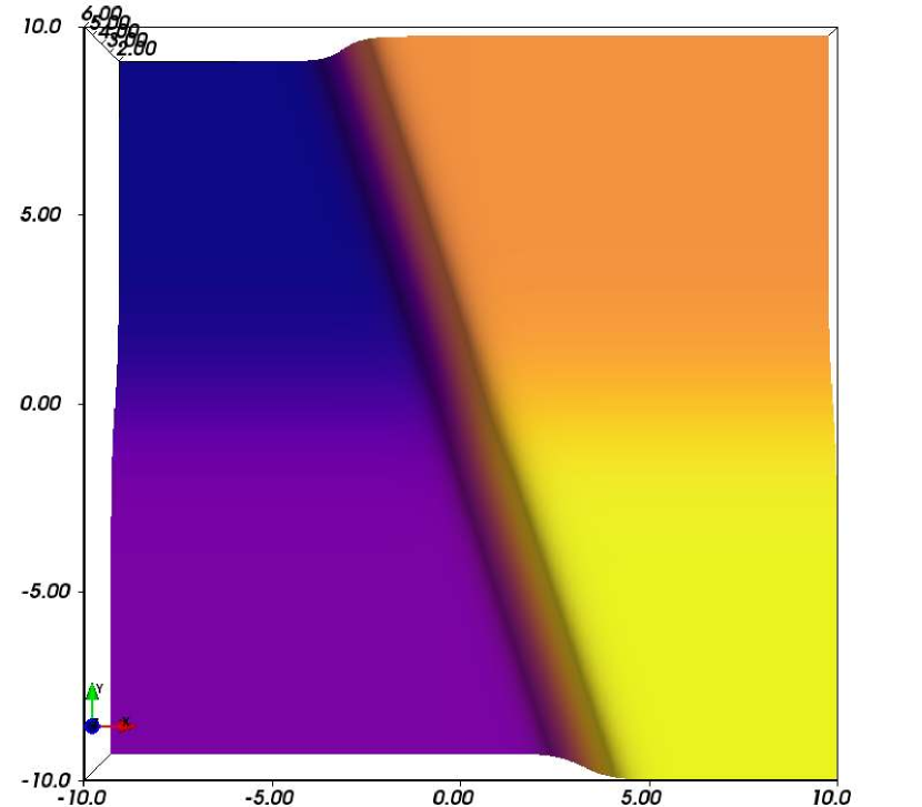
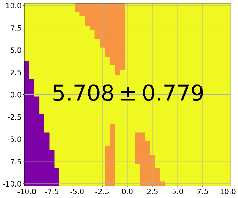
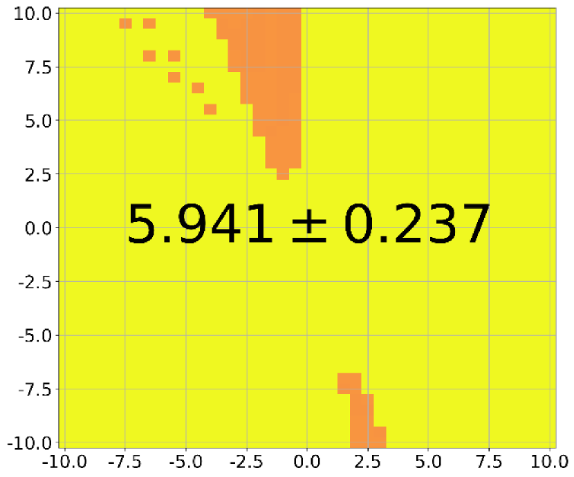
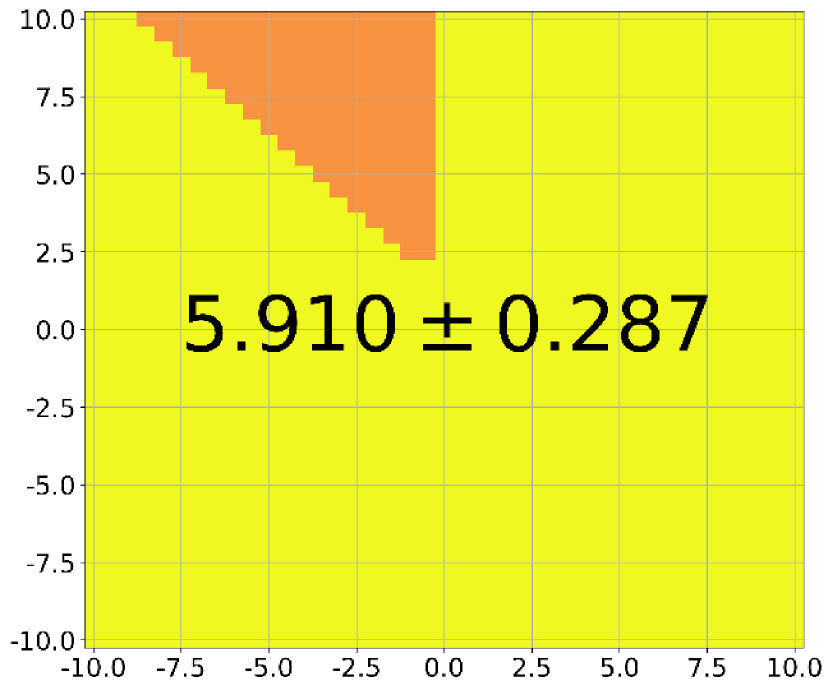
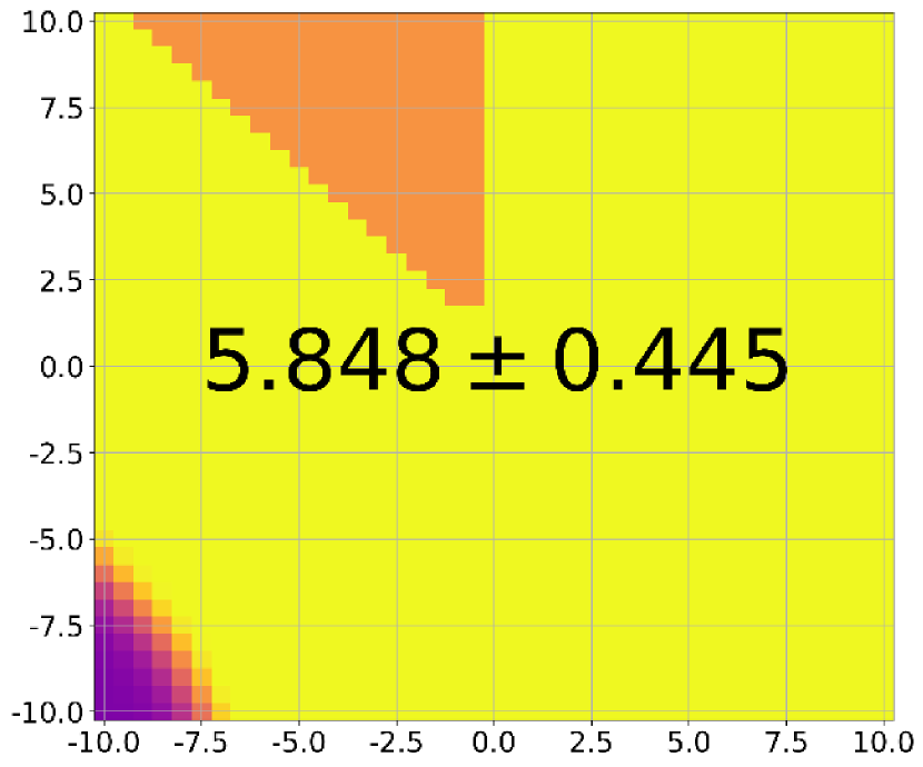
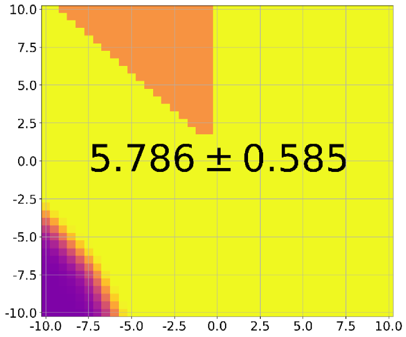
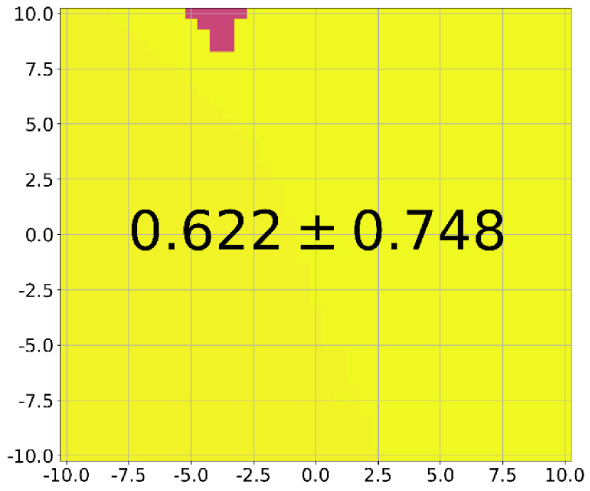
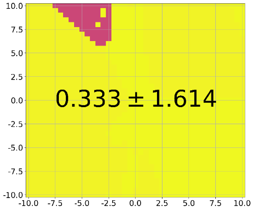
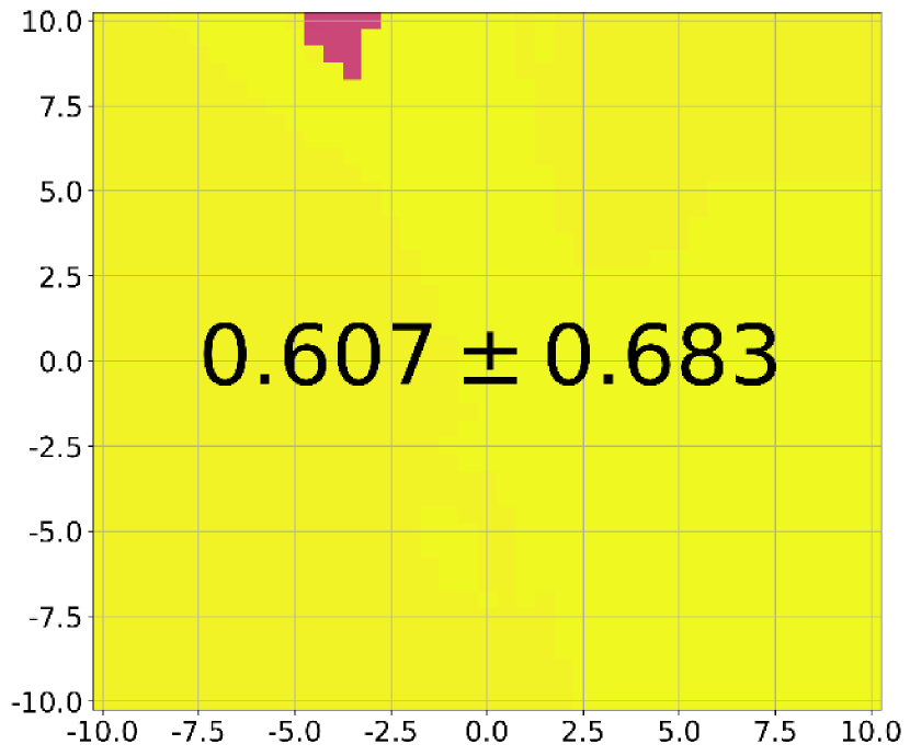
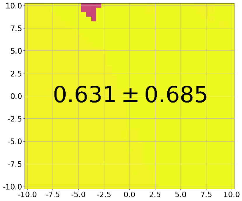
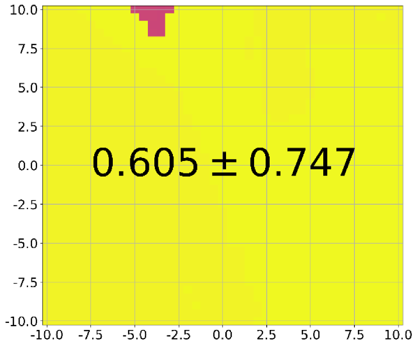
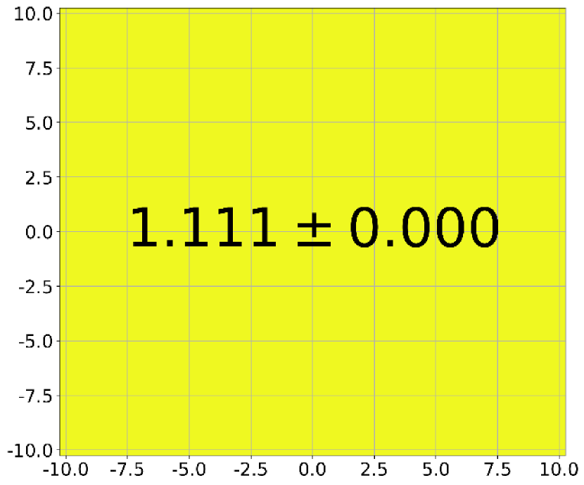
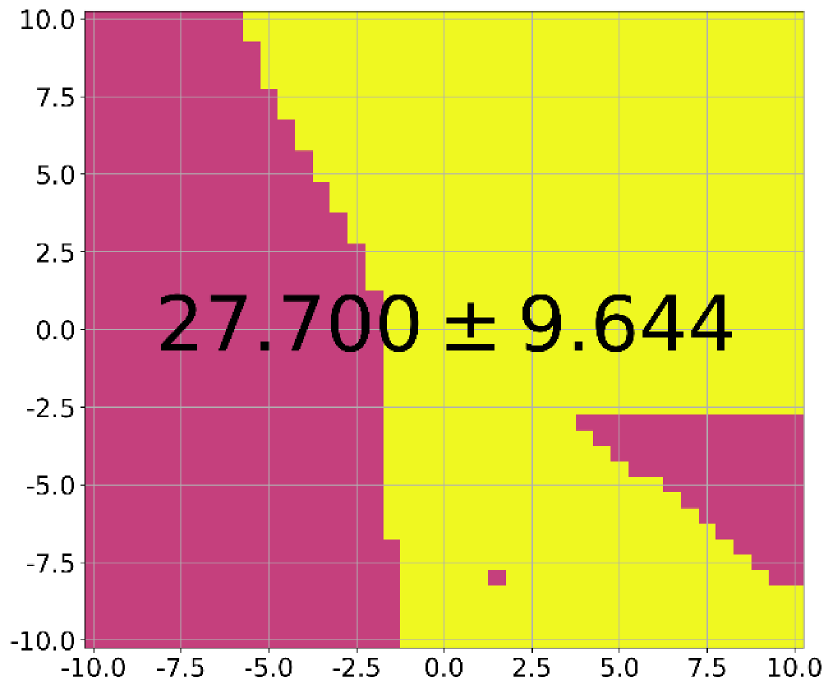
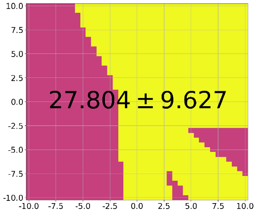
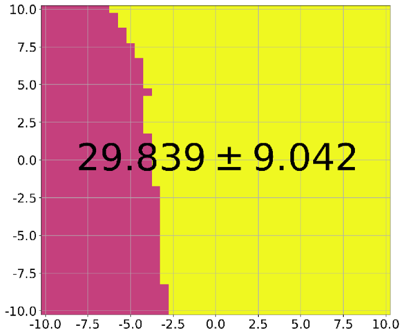
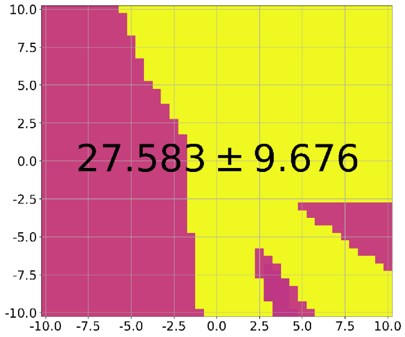
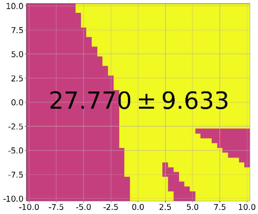
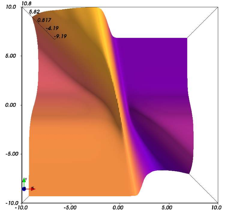
(a) Bias landscape

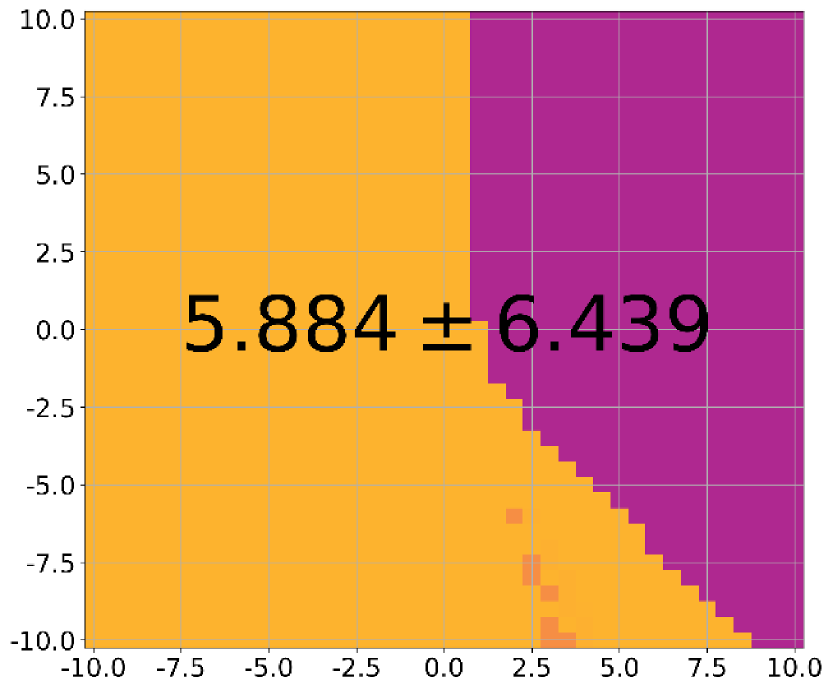
(b) Devmat

(c) Analytic (18)

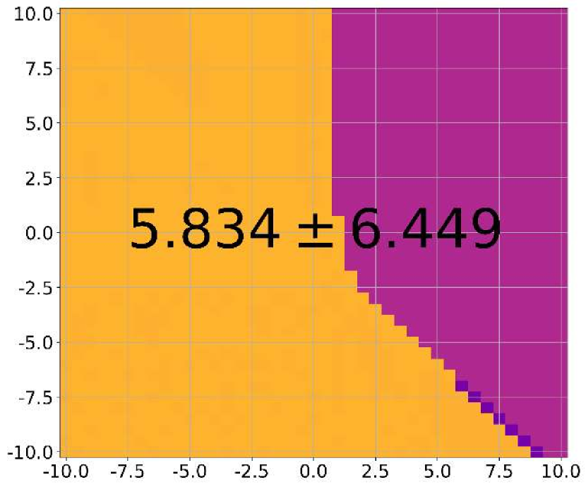
(d) $\hat{t}_{\mathrm{abs:min}}=1$

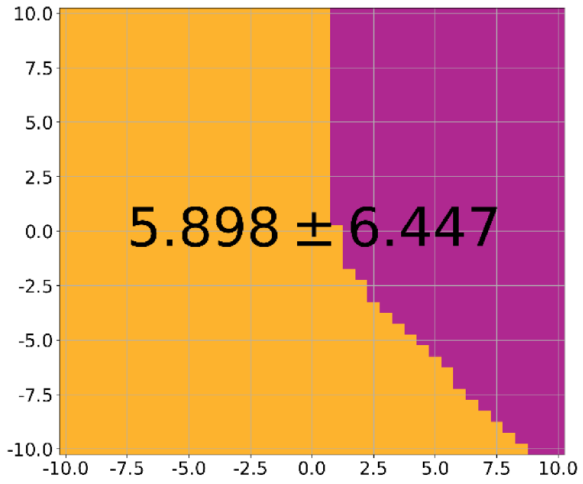
(e) $\hat{t}_{\mathrm{abs:min}}=2$

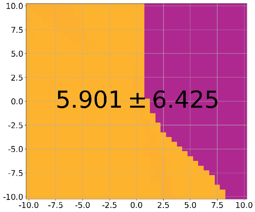
(f) $\hat{t}_{\mathrm{abs:min}}=3$

(g) $\hat{t}_{\mathrm{abs:min}}=4$

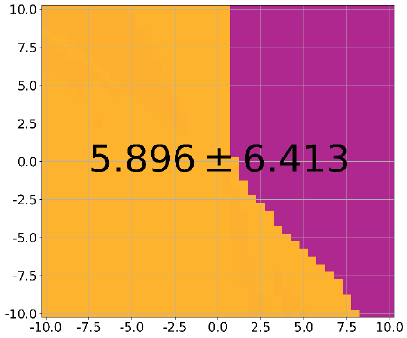
(h) $\hat{t}_{\mathrm{abs:min}}=5$

Figure 9: A comparison of Fisher candidates for exact bias-only optimization on Env-A1, A2, A3, B1, B2, and B3 (top to bottom rows). The Devmat Fisher uses the entry-wise absolute deviation matrix, that is, $\sum_{s\in\mathcal{S}}|h_{\pi}(s|s_{0})|\boldsymbol{\Phi}_{\!a}(\boldsymbol{\theta},s)$. The Analytic Fisher refers to Scheme iii. (Sec 7.3). Both Devmat and Analytic candidates do not enable sampling-based approximation. Contrarily, the other five candidates are sampling-enabler expressions (but computed exactly here). They are derived from (19) with varying minimum absorption time estimates $\hat{t}_{\mathrm{abs:min}}=1,2,\ldots,5$ (each is invariant to policies and initial states). Like in Fig 8, the color indicates the bias of the final policy parameter from optimization initialized at the corresponding 2D-coordinate. It maps low bias to dark-blue, whereas high bias to yellow. Each subplot has $1681$ final bias grid-values, whose mean and standard deviation are indicated by the number in the middle. Here, the highest final bias (yellow color) is desirable. For experimental setup, see Sec 6.

In exact settings, we also carried out comparisons on seven different bias Fisher candidates for bias-only optimization. This is to track the empirical effects of the series of approximation (not including sampling-based approximation) that lead to the sampling-enabler bias Fisher in (19). As can be seen in Fig 9, the use of $\sum_{t=0}^{\infty}|p_{\pi}^{t}(s|s_{0})-p_{\pi}^{\star}(s)|$, in lieu of $|h_{\pi}(s|s_{0})|$ in (18), does not significantly degrade the advantage of the Fisher. Then, dropping some terms in (18) causes acceptable degradation as anticipated. It is interesting that increasing $\hat{t}_{\mathrm{abs:min}}$ (i.e. dropping fewer terms in (18)) does not always result in better optimization performance as in Env-A2 and A3. We observe that $\hat{t}_{\mathrm{abs:min}}=2$ gives us the best compromise across at least, six benchmarking environments (Sec 6.1).

In sampling-based approximation settings, the stochastic natural gradients outperform the stochastic standard gradients whenever the sample size is sufficient in order to obtain sufficiently accurate estimates of the Fisher matrix. Note that the behavior of sampling-based approximation is a function of sample sizes, following the strong law of large numbers. Recall that if $Y_{1},\ldots,Y_{m}$ are i.i.d random variables, then the deviation between the sample mean $\bar{Y}\coloneqq\frac{1}{m}\sum_{i=1}^{m}Y_{i}$ and its expectation $\mathbb{E}\mathopen{}\mathclose{{}\left[\bar{Y}}\right]=\mathbb{E}\mathopen{}\mathclose{{}\left[Y_{i}}\right]$ (due to unbiasedness of the sample mean) is of order $\mathcal{O}\mathopen{}\mathclose{{}\left(1/\sqrt{m}}\right)$. Assuming that $Y_{i}\in[y_{min},y_{max}]$ almost surely and for $\delta\in(0,1)$, with probability greater than $1-\delta$, we have $|\bar{Y}-\mathbb{E}\mathopen{}\mathclose{{}\left[Y_{i}}\right]|\leq|y_{min}-y_{max}|\sqrt{\frac{\log(2/\delta)}{2m}}$, which is derived through the Hoeffding’s inequality.

7.4 Initial barrier parameter tuning

The proposed Algo 1 requires an initial value of the barrier parameter $\beta_{0}$. For tuning $\beta_{0}$, we run the exact version of Algo 1 several times with $\beta_{0}\in\{0.01,0.1,1,10,100,1000,10000\}$ representing a range of values from small to large extremes. We note that in general, the value of $\beta_{0}$ goes hand in hand with the shrinking parameter $\beta_{\mathrm{div}}$ and the number of outer iterations in Algo 1. For a recipe for choosing those parameters’ values, we refer the reader to boyd_2004_cvxopt and bertsekas_1996_copt. Also note that the barrier parameter $\beta$ is quite analogous to the penalty parameter of penalty methods, such as the penalty parameter $\phi$ in (27).

Fig 10 shows the experimental results on Env-A1, A2, A3, B1, B2, and B3. For Env-A, a small $\beta_{0}$ yields best performance (i.e. lowest absolute bias error: the blue color). This is expected because all policies of Env-A are gain optimal. In model-free RL, if we knew that the gain landscape is flat, then we would optimize only the bias without the barrier by setting $\beta_{0}\leftarrow 0$. Thus for this kind of environments, values towards the small extreme are suitable for $\beta_{0}$. Note that in exact settings, $\beta_{0}$ matters to the gradient-ascent update only through the multiplication of $\beta$ with the gain Fisher $\boldsymbol{\Phi}_{\!ga}$ as in (26). This is because the gain gradient $\nabla g(\boldsymbol{\theta})$ is a zero vector for Env-A.

On the other hand for Env-B, values towards the large extreme are suitable for $\beta_{0}$. As mentioned in Sec 5, a small $\beta_{0}$ tends to induce ill-conditioned bias-barrier optimization landscapes, which should be avoided in the early outer iterations of Algo 1. Recall that for Env-B the barrier function is essential since such an environment type requires gain-then-bias-barrier bi-level optimization.

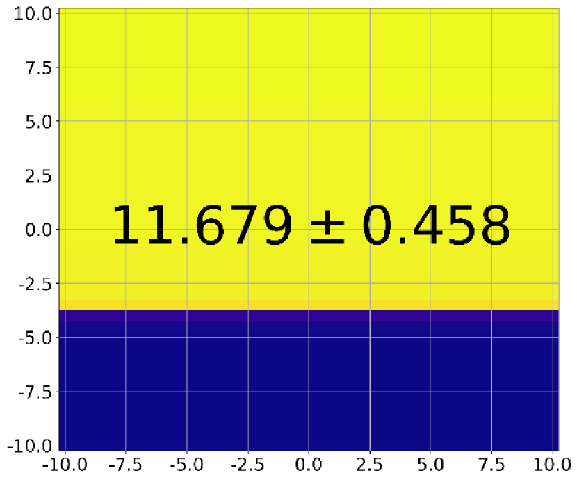
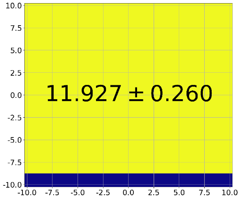
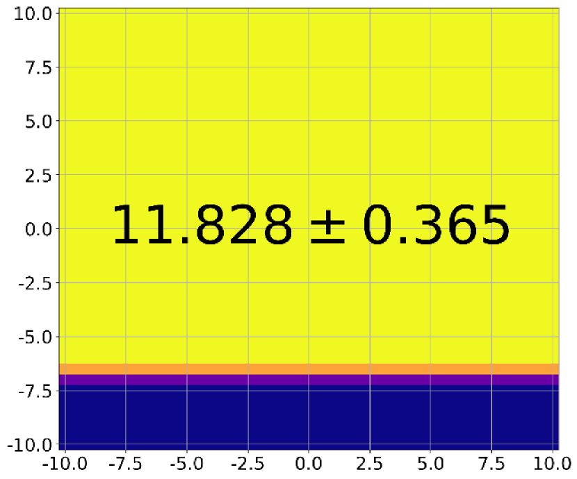
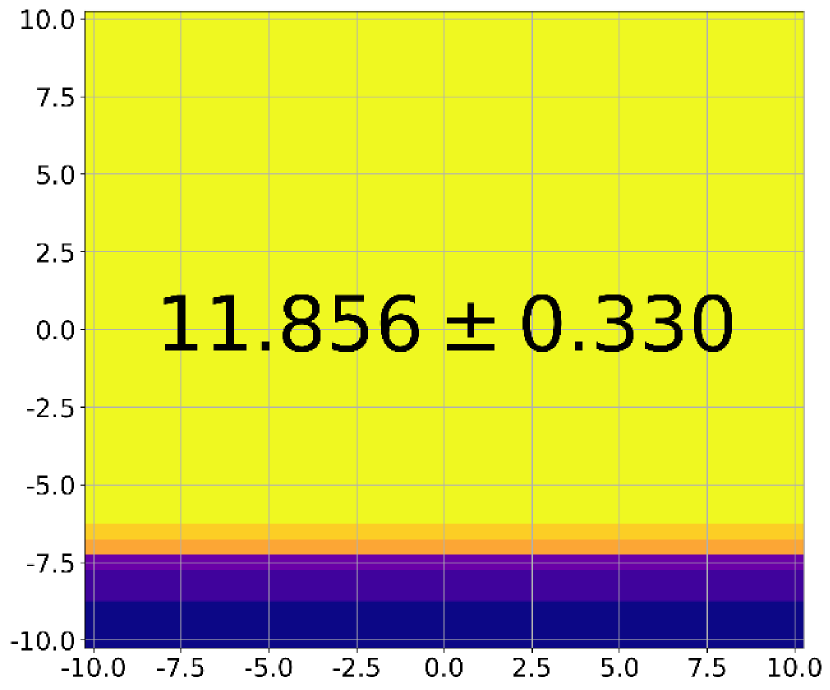
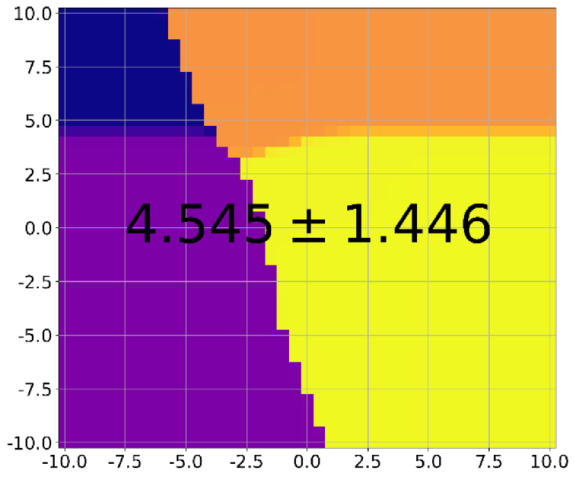
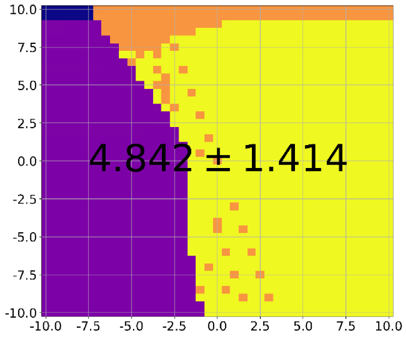
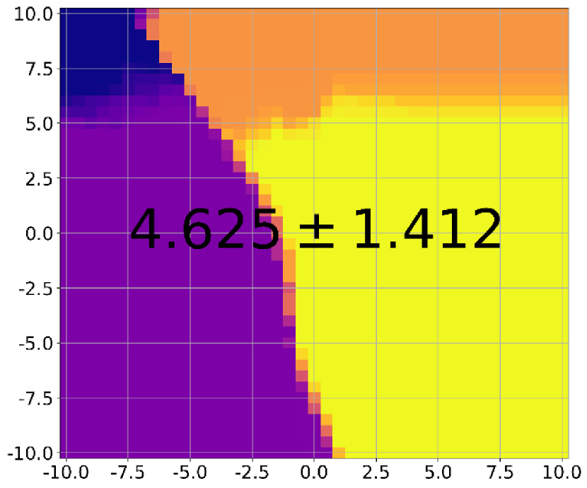
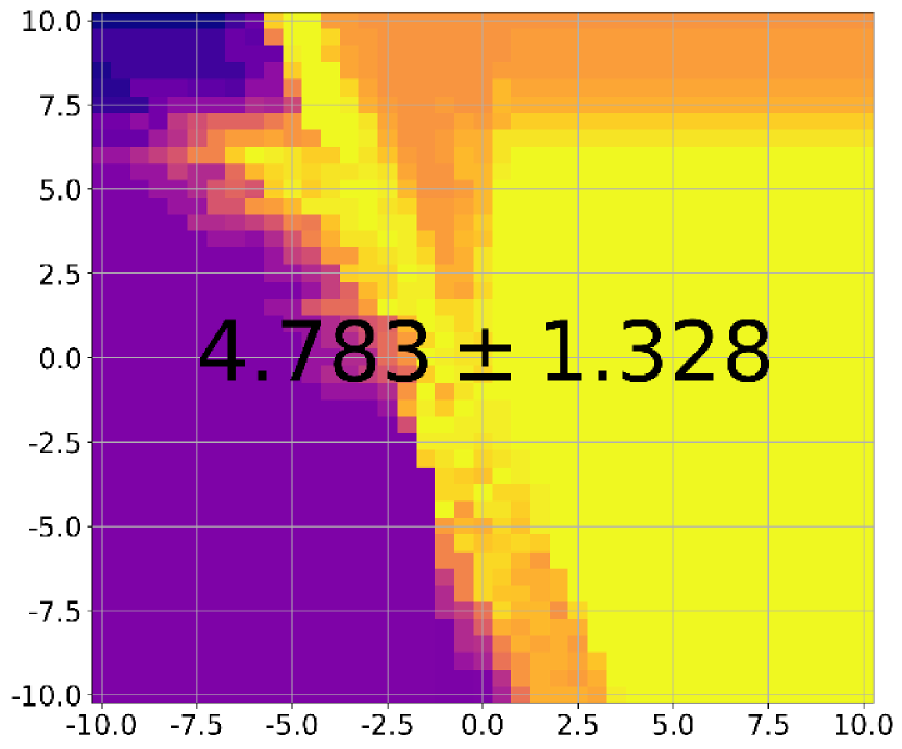
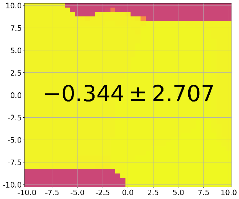
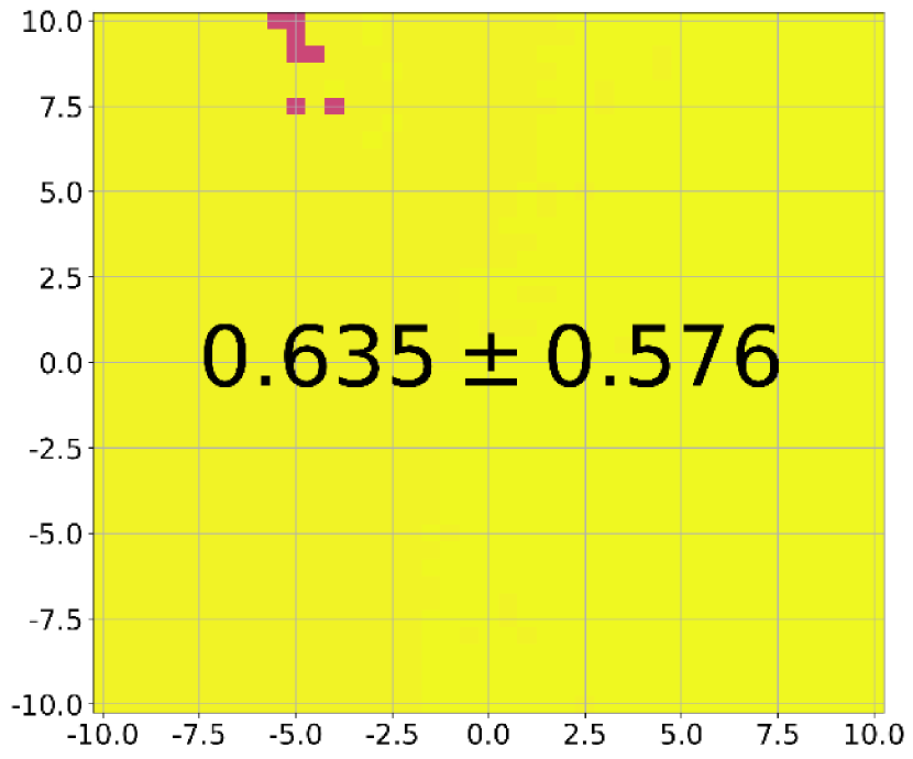
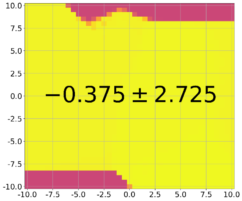
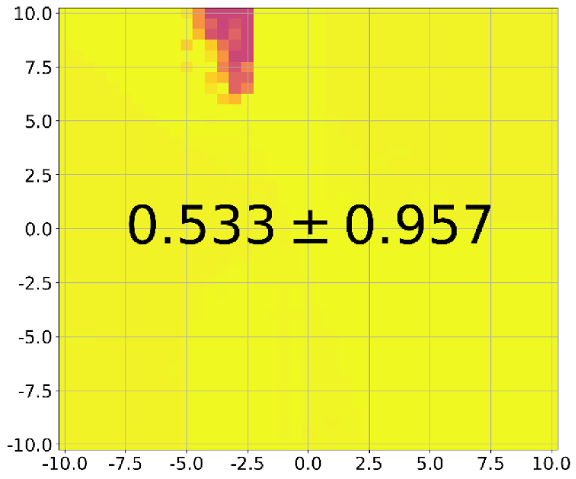
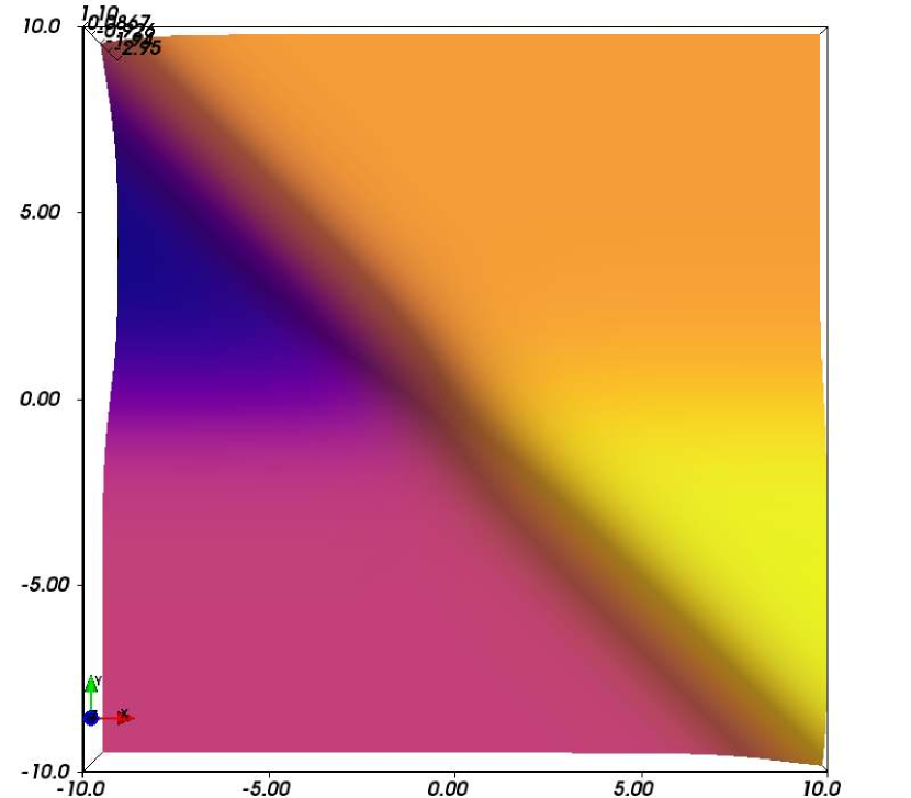
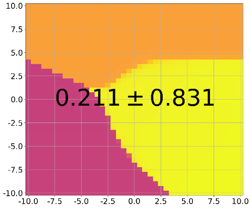
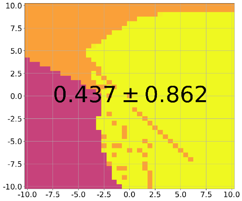
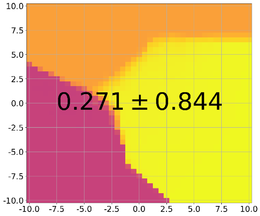
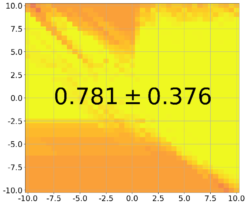
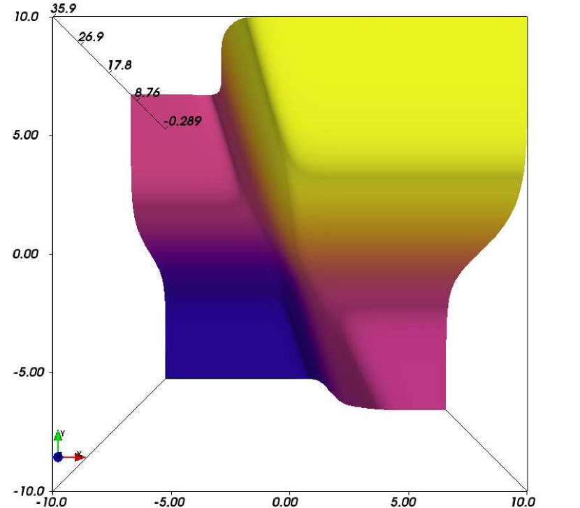
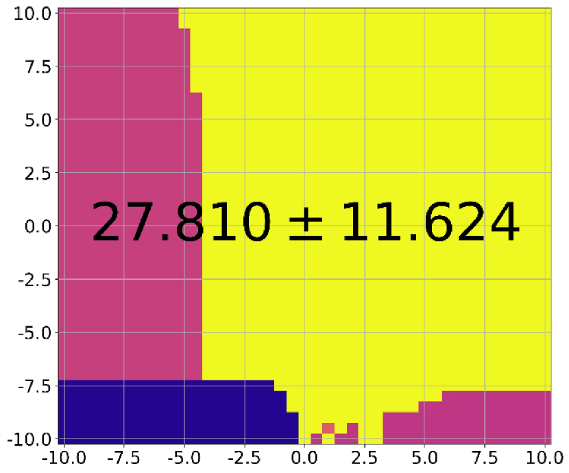
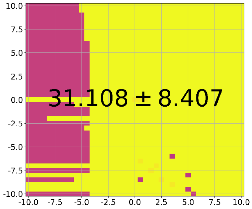
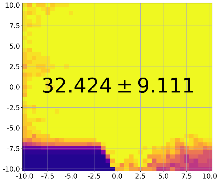
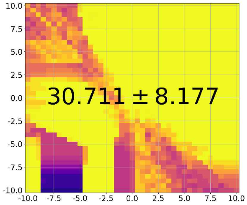
(a) Bias landscape

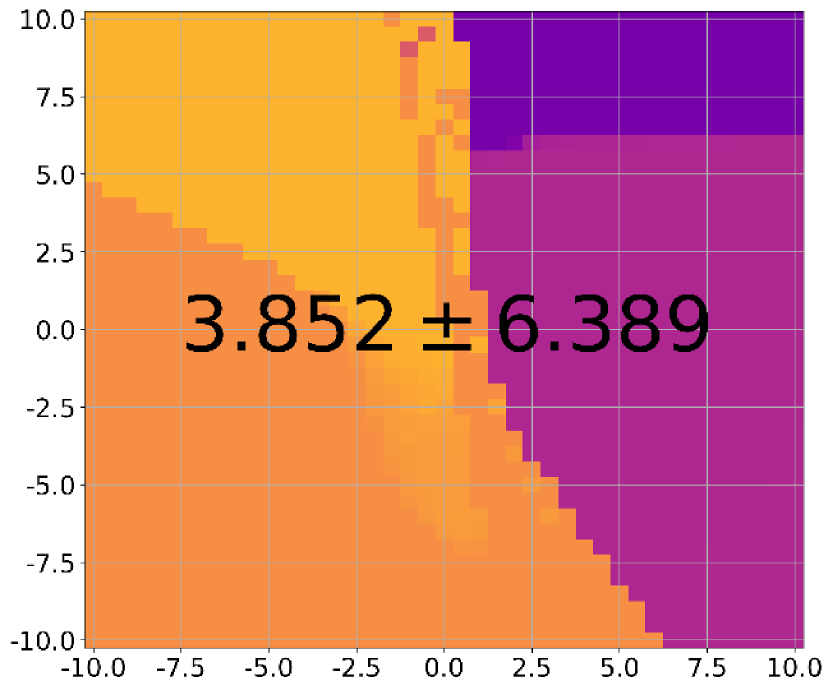
(b) Identity

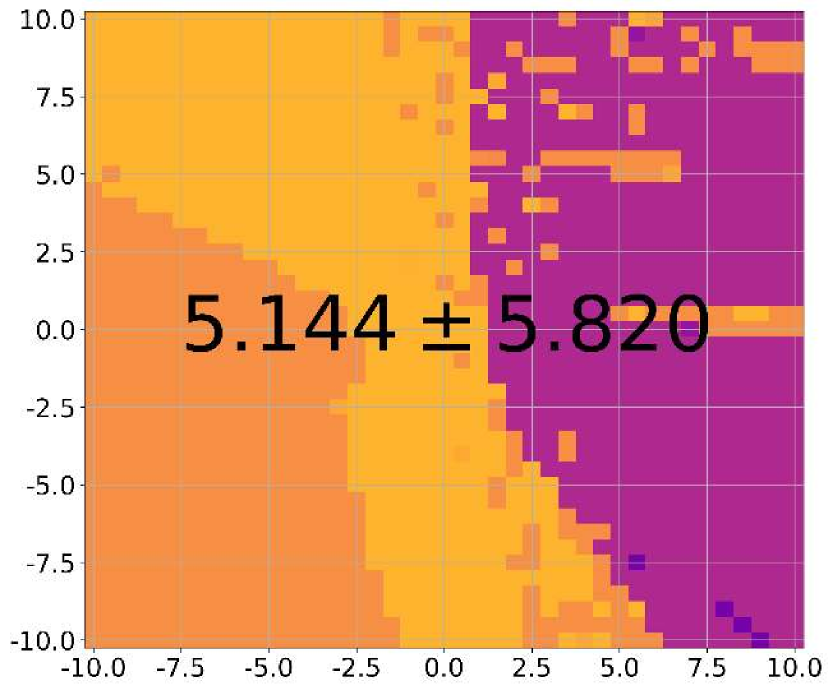
(c) (Modified) Hessian

(d) Analytic Fisher

(e) Sampling Fisher

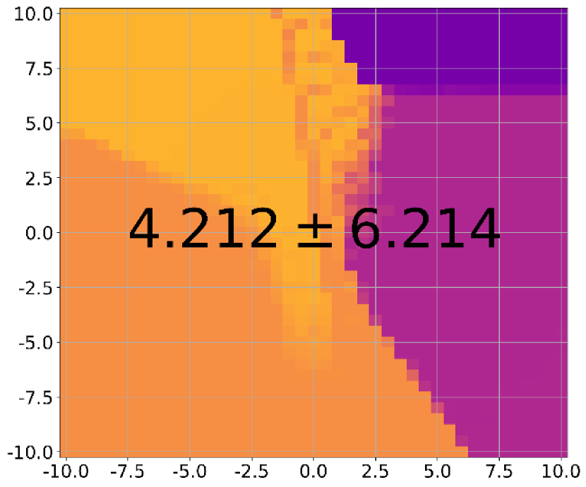
(f) 16-sample Identity

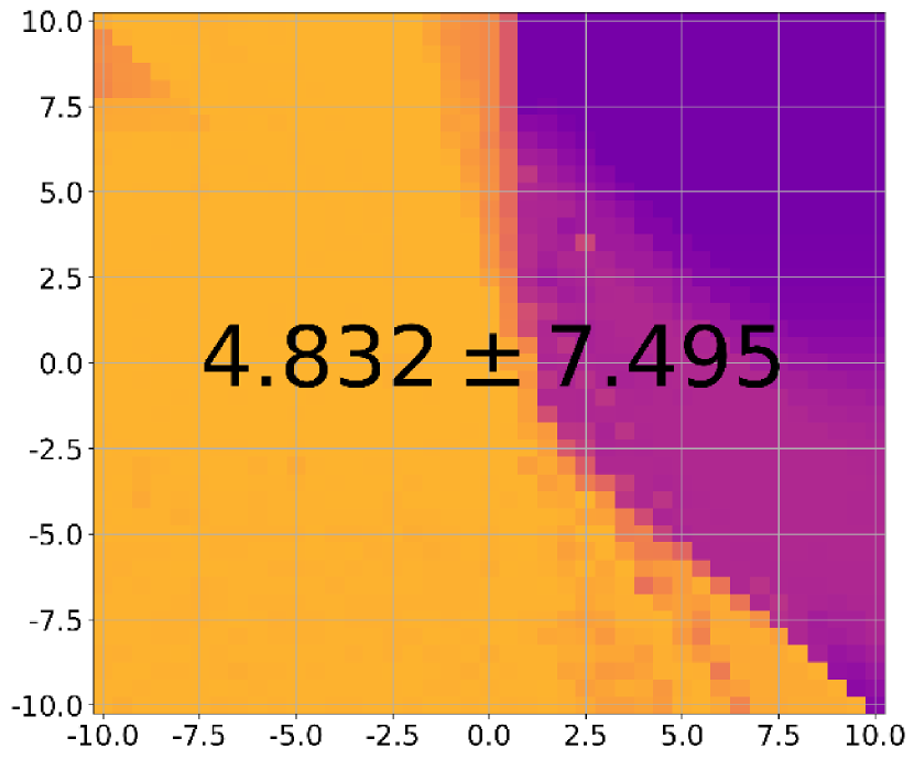
(g) 16-sample Fisher

Figure 8: Bias-only optimization on Env-A1, A2, A3, B1, B2, and B3 (top to bottom rows). The 2nd to 5th columns from the left correspond to exact optimization of Schemes i, ii, iii, and iv, whereas the two right-most columns correspond to sampling-based approximation of Schemes i and iv (with 10 random seeds), as explained in Sec 7.3. The color indicates the bias $v_{b}(\boldsymbol{\theta},s_{0})$ of the final policy parameter $\boldsymbol{\theta}$ from optimization initialized at the corresponding 2D-coordinate as $\boldsymbol{\theta}_{0}$. It maps low bias to dark-blue, whereas high bias to yellow. Each subplot has $1681$ final bias grid-values, whose mean and standard deviation are indicated by the number in the middle. Here, the highest final bias (yellow color) is desirable. For experimental setup, see Sec 6.

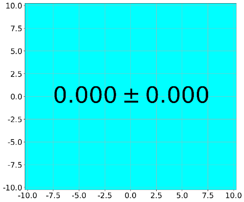
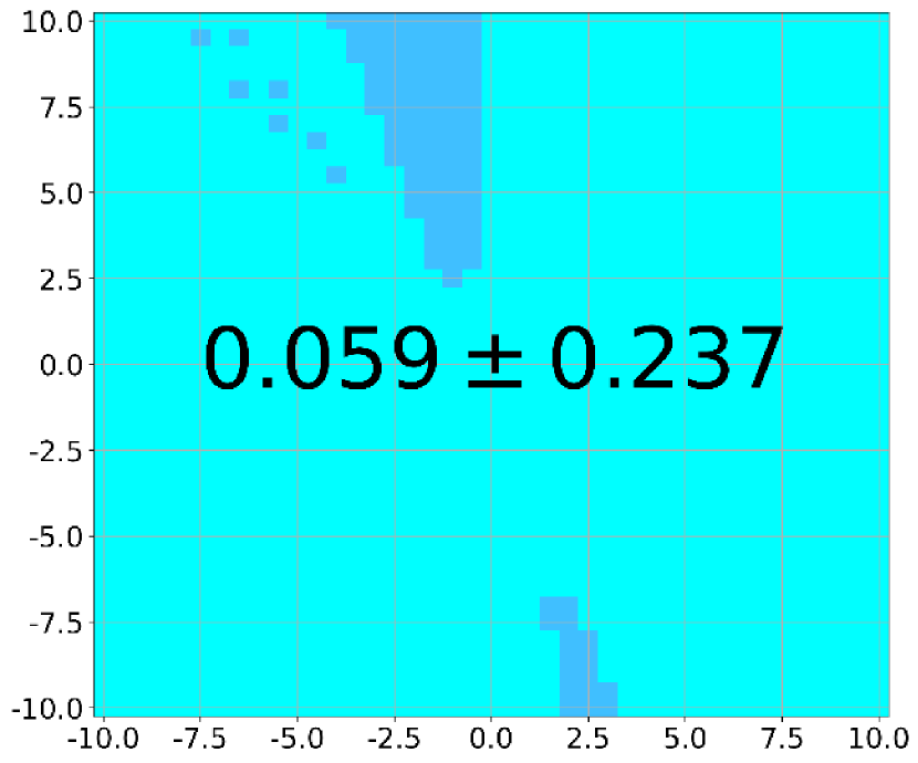
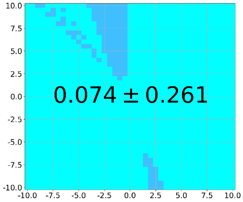
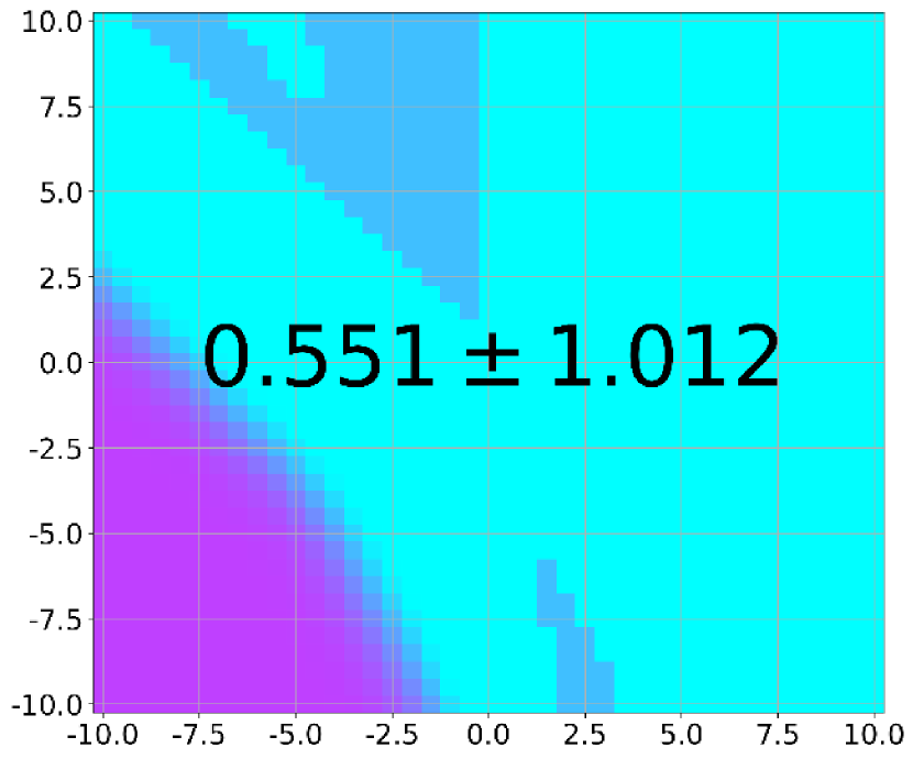
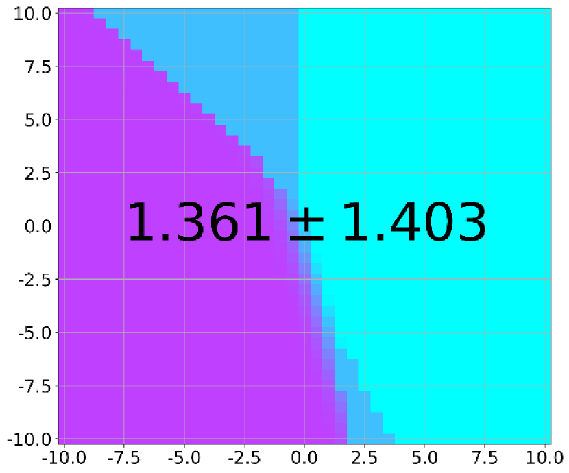
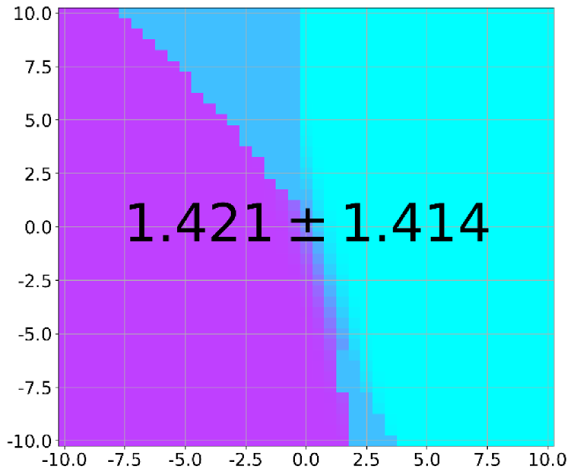
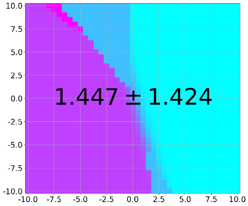
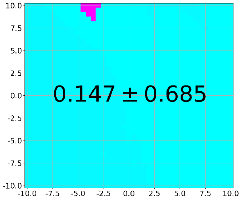
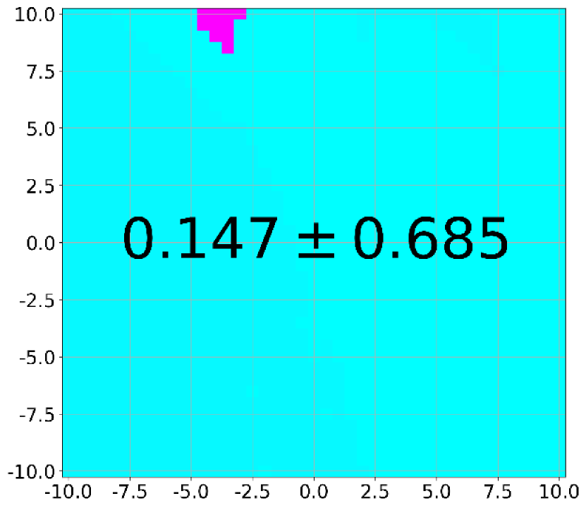
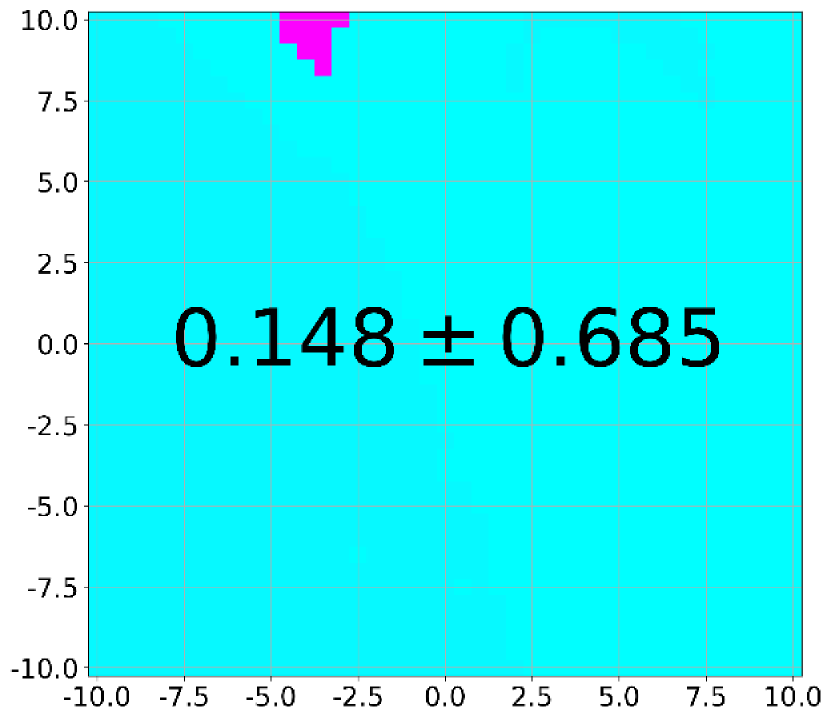
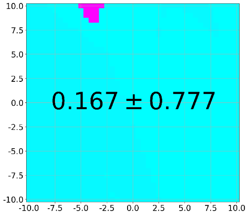
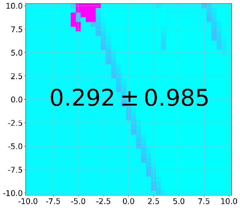
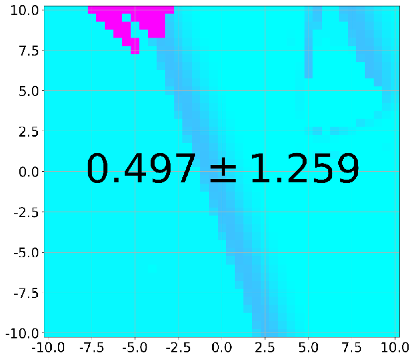
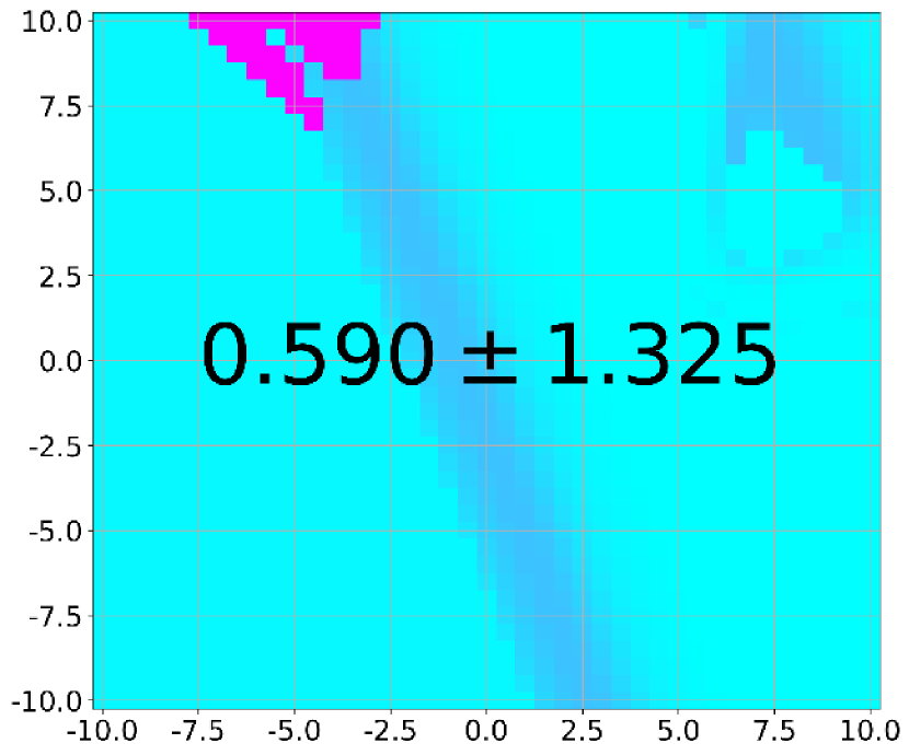
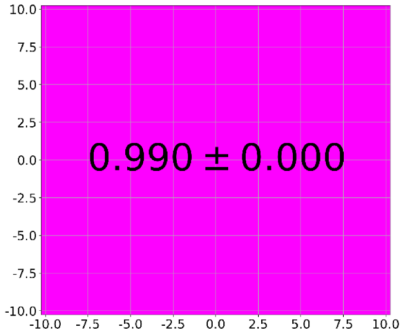
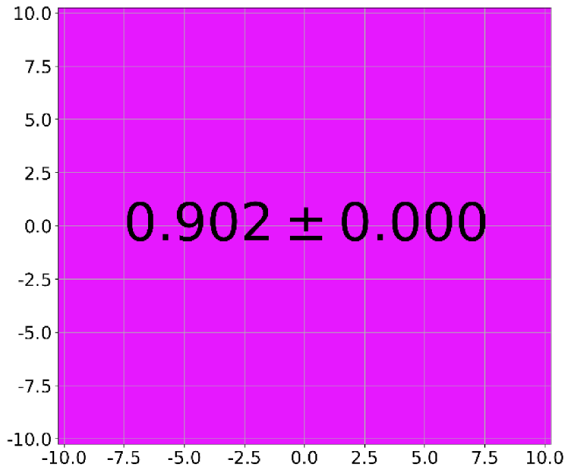
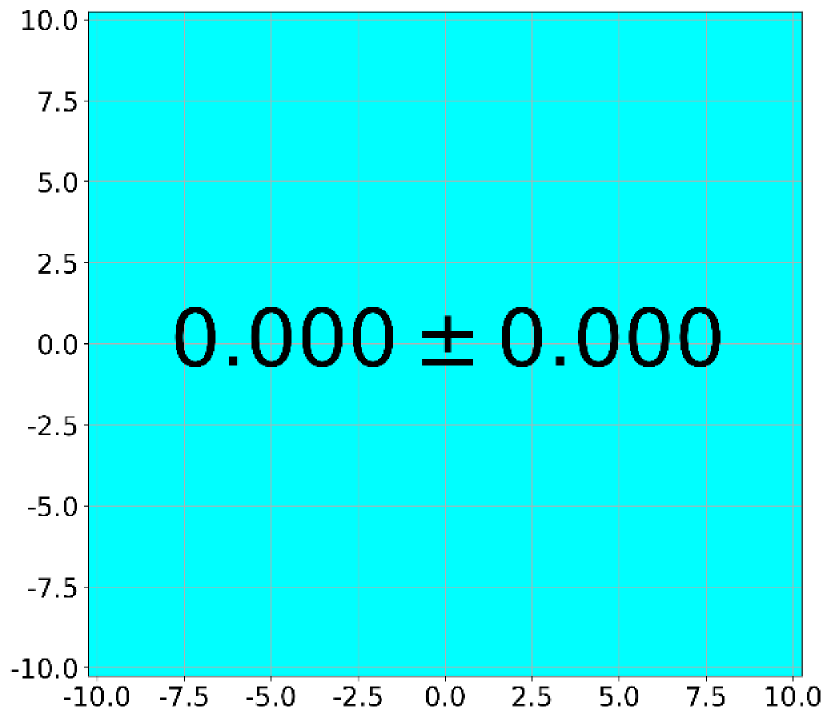
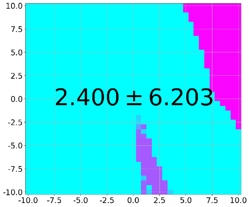
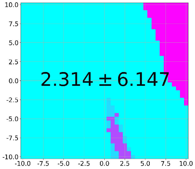
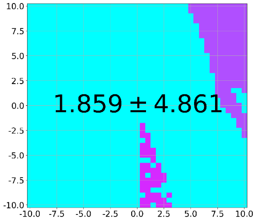
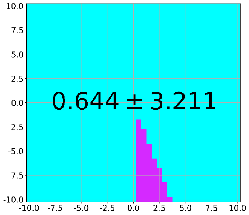
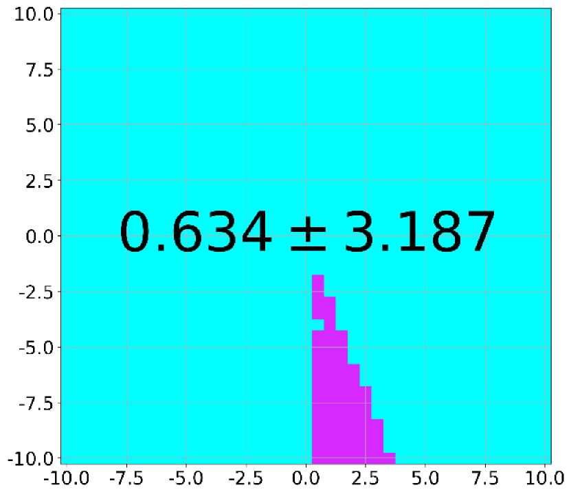
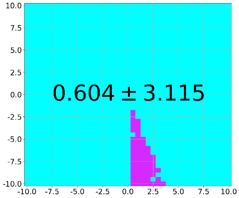
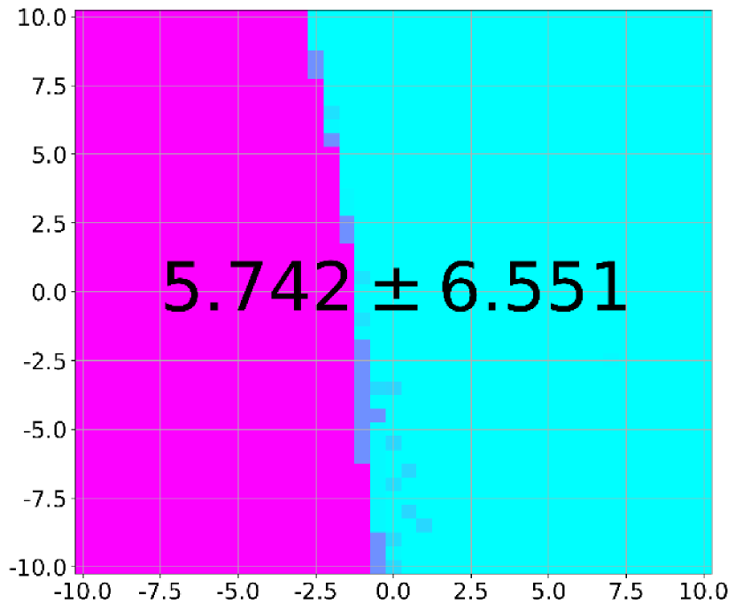
(a) $\beta_{0}=0.01$

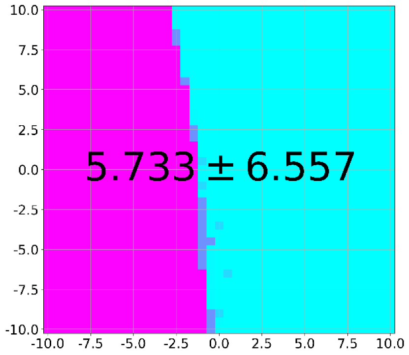
(b) $\beta_{0}=0.1$

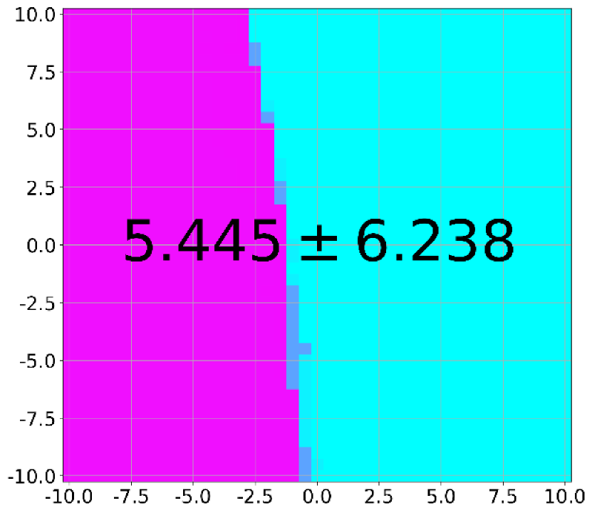
(c) $\beta_{0}=1.0$

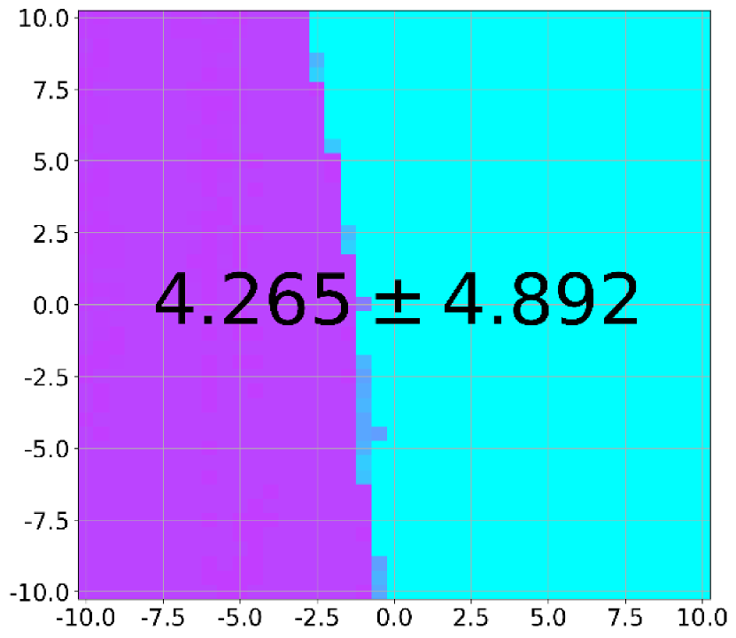
(d) $\beta_{0}=10.0$

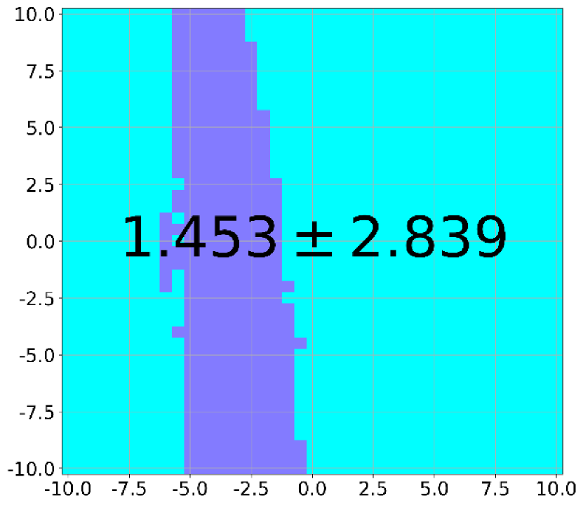
(e) $\beta_{0}=100.0$

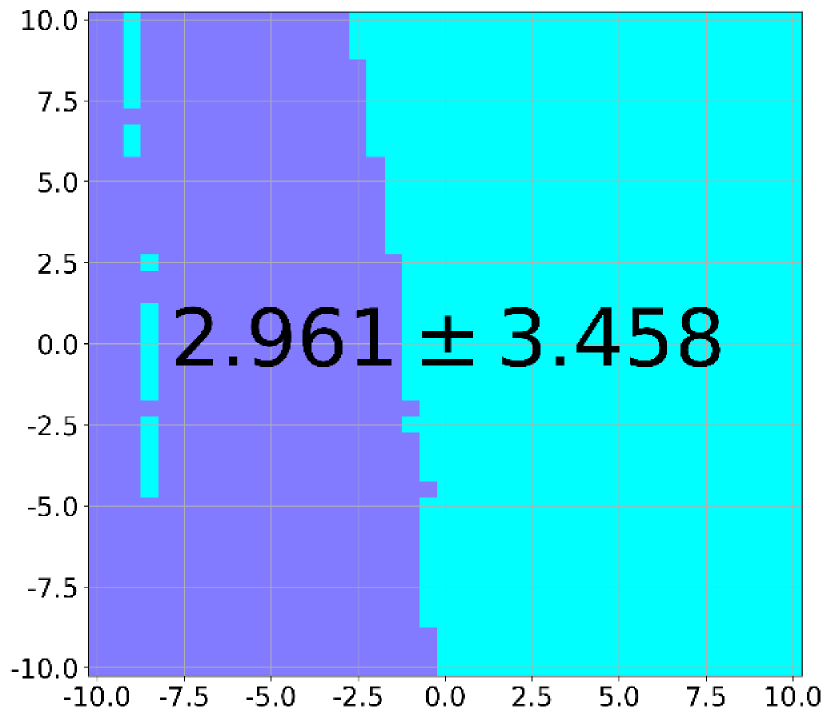
(f) $\beta_{0}=1000.0$

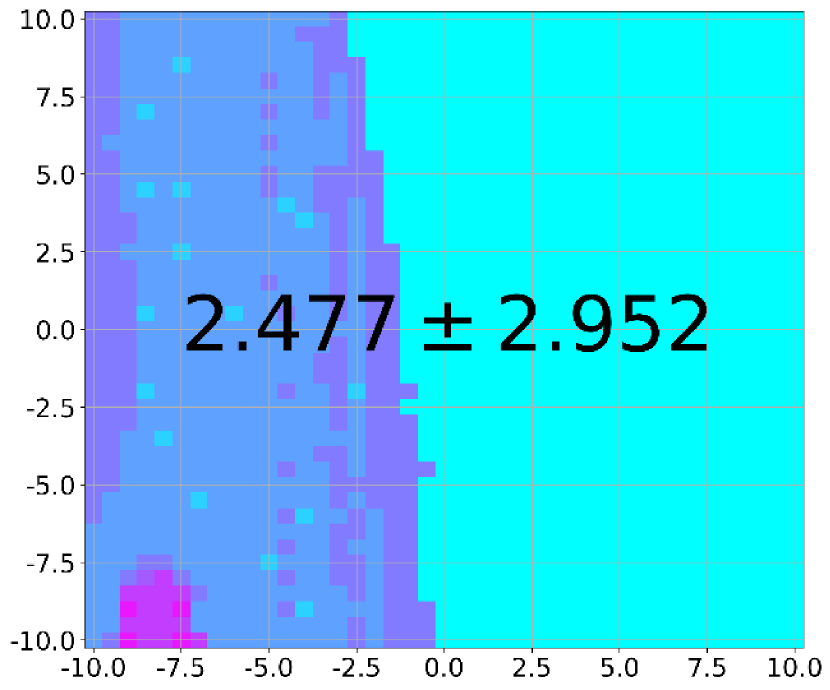
(g) $\beta_{0}=10000.0$

Figure 10: Tuning the initial barrier parameter $\beta_{0}$ on Env-A1, A2, A3, B1, B2, and B3 (top to bottom rows) using the exact variant of Algo 1. Like in Fig 6, each subplot shows the absolute difference (low:blue to high:magenta) between the bias of the nBw-optimal deterministic policy and of the resulting randomized policy, where the 2D-coordinate indicates the initial policy parameter value. In each subplot, the numbers in the middle indicate the mean and standard deviation across $1681(=41^{2})$ grid values. Here, the lowest absolute bias difference (blue) is desirable. For experimental setup, see Sec 6.

8 Related works

Table 2: Model-free RL works that target nBw-optimal policies in unichain MDPs. This table lists two criteria: $\gamma$-discounted and $n$-discount optimality, as well as two algorithmic styles: value- and policy-iteration methods. Here, $\gamma_{\mathrm{Bw}}$ denotes the so-called Blackwell’s discount factor as in (34).

Styles \ Criteria	$\gamma$-discounted with $\gamma\in[\gamma_{\mathrm{Bw}},1)$	$n$-discount with $n\geq 0$
Value iteration	schneckenreither_2020_avgrew	mahadevan_1996_sensitivedo
Policy iteration	None	Our work

In order to classify the existing literature, we need to review two approaches to obtaining nBw-optimal policies in unichain MDPs. First is through $n$-discount optimality criterion with $n\geq 0$. Here, a policy $\pi_{n}^{*}$ for $n=-1,0,1,\ldots$, is $n$-discount optimal if

$$\lim_{\gamma\uparrow 1}\frac{1}{(1-\gamma)^{n}}\Big{(}v_{\gamma}(\pi_{n}^{*},s)-v_{\gamma}(\pi,s)\Big{)}\geq 0,\qquad\forall\pi\in\Pi_{\mathrm{S}},\forall s\in\mathcal{S},\ \text{and $v_{\gamma}(\pi,s)$ defined in \eqref{equ:disrew_v}}.$$

A policy is said to be ($n=\infty$)-discount optimal if it is $n$-discount optimal for all $n\geq-1$. Second is through $\gamma$-discounted optimality criterion with a discount factor $\gamma$ that lies in the so-called Blackwell’s interval. That is, $\gamma\in[\gamma_{\mathrm{Bw}},1)$, where $\gamma_{\mathrm{Bw}}\coloneqq\sup_{s\in\mathcal{S}}\gamma_{\mathrm{Bw}}(s)$. Here, $\gamma_{\mathrm{Bw}}(s)$ comes from the definition of Blackwell optimality: a policy $\pi^{*}_{\mathrm{Bw}}$ is Blackwell optimal if for each $s\in\mathcal{S}$, there exists a $\gamma_{\mathrm{Bw}}(s)$ such that

$$v_{\gamma}(\pi^{*}_{\mathrm{Bw}},s)\geq v_{\gamma}(\pi,s),\qquad\text{for}\ \gamma_{\mathrm{Bw}}(s)\leq\gamma<1,\text{and for all}\ \pi\in\Pi_{\mathrm{S}}.$$ (34)

Intuitively, the Blackwell optimality claims that upon considering sufficiently far into the future via $\gamma\geq\gamma_{\mathrm{Bw}}$, there is no policy better than the Blackwell optimal policies (denis_2019_bwopt).

The above two approaches are based on the fact that ($n=y$)-discount optimality implies ($n=x$)-discount optimality for all $y>x$, and on the equivalency between the nearly-Blackwell (nBw, bias) and $(n=0)$-discount optimality criteria, as well as between the Blackwell and $(n=\infty)$-discount optimality criteria (puterman_1994_mdp, Thm 10.1.5).

Since $\gamma_{\mathrm{Bw}}$ is generally unknown in RL, the main challenge in obtaining nBw-optimal policies through $\gamma$-discounted optimality is to specify the discount factor $\gamma$. It should not be too far from 1, otherwise it is likely that $\gamma<\gamma_{\mathrm{Bw}}$. Simultaneously, $\gamma$ should not be too close to 1 because a higher $\gamma$ typically leads to slower convergence (even-dar_2004_qlr). Moreover, as $\gamma$ approaches 1, the induced $\gamma$-discounted optimality yields optimal policies similar to those of gain optimality (which is underselective in unichain MDPs). This implies that determining $\gamma$ is more difficult in unichain than recurrent MDPs, for which the gain optimality (equivalently, ($n=-1$)-discount optimality) is already the most selective. We therefore do not discuss works that manipulate $\gamma$ towards achieving Blackwell optimality but are limited to recurrent MDPs.

Table 2 shows model-free RL works that target nBw-optimal policies in unichain MDPs. It classifies the works based on whether they optimize $\gamma$-discounted or $n$-discount optimality criteria, as well as whether they follow value- or policy-iteration algorithmic styles. We found a relatively few works on this area. The closest to our work is that of mahadevan_1996_sensitivedo, then the work of schneckenreither_2020_avgrew. Both use tabular policy representation, which can be interpreted as a special case of policy parameterization used in this work. For discussion on (mahadevan_1996_sensitivedo), refer to Sec 1.

schneckenreither_2020_avgrew introduced a novel notion of discounted state values that are adjusted by the gain. The action selection utilizes an $\epsilon$-sensitive lexicographic order that operates in two gain-adjusted discounted state-values with two different discount factors, i.e. $0.5\leq\gamma_{0}<\gamma_{1}\leq 1$. Here, those two discount factors $\gamma_{0},\gamma_{1}$ and such a comparison measure $\epsilon$ are hyperparameters.

We are not aware of any work based on policy-iteration that deliberately aims for Blackwell optimality via the $\gamma$-discounted approach. There are (many) works that fine-tune $\gamma$, for instance, those by zahavy_2020_stdrl; paul_2019_hoof; xu_2018_mgrad. Their tuning metrics however are not clearly motivated by Blackwell optimality such that no concept of Blackwell’s interval is involved. Hence, we argue that they are beyond our current scope.

9 Conclusions, limitations and future works

We propose a policy gradient method that can obtain nearly-Blackwell (bias) optimal policies. It extends the existing average-reward methods in that it performs further selection among the resulting (approximately) average-reward (gain) optimal policies. This is carried out through optimizing a function of the bias and an RL-specific logarithmic barrier. The corresponding stochastic optimization utilizes a novel expression that enables sampling for natural gradients of the bias. Experiment results validate the viability of our proposed method, which can be regarded as a first step towards attaining $n$-discount optimality through RL for $n\geq 0$.

Next, we identify some limitations of our proposed method. They are described along with possible follow-up works that address them but are left for future works.

Obtaining unbiased estimates of the gradient (4) and the Fisher matrix (19) of the bias requires some knowledge (or a satisfied assumption) about the mixing time. That is, the process is mixing before or at the last timestep of an experiment-episode (trial). It is likely useful therefore to have a policy gradient agent that can control the magnitude of the mixing time, such as the one proposed by morimura_2014_pgrl. The mixing-time control can be implemented for example, in the form of regularization in the gain and bias-barrier objective functions such that the policy iterate $\pi$ induces one-step transition matrix $\boldsymbol{P}_{\!\!\pi}$ whose mixing time is low. Note that the issue of sampling states from a stationary state distribution (which appears after mixing) is also present in the average-reward case in order to obtain unbiased gradient estimates. In the discounted-reward case, this corresponds to sampling states from the discounted state distribution (30).

The proposed Algo 1 has not been analysed in terms of its sample complexity. The challenge comes from the fact that it is stochastic barrier optimization with potentially biased samples, for instance due to Markovian (not independent) state samples and/or due to sampling from a distribution that is not identical to the stationary state distribution. Moreover, there is a finite number of visitations to transient states in a single experiment-episode. It is therefore imperative to be able to derive a finite sample complexity (non-asymptotic convergence) of the proposed method. Apart from the analysis, the sample complexity may be reduced in several ways, including a) iterative techniques for computing the inverse of the Fisher matrix, b) action-independent baseline substraction for the gradients, and c) action-value function approximators for the gradients (as in the following passage).

Our proposed Algo 1 also has not been incorporated with any function approximator for estimating the action values, which are used in the bias gradients (4). Particularly here, the function approximator is required to estimate the policy values from both transient and recurrent states (note that typical approximators are designed to estimate policy values only from recurrent states).