Pseudo-marginal inference for CTMCs on infinite spaces via monotonic likelihood approximations

Abstract

Bayesian inference for Continuous-Time Markov Chains (CTMCs) on countably infinite spaces is notoriously difficult because evaluating the likelihood exactly is intractable. One way to address this challenge is to first build a non-negative and unbiased estimate of the likelihood—involving the matrix exponential of finite truncations of the true rate matrix—and then to use the estimates in a pseudo-marginal inference method. In this work, we show that we can dramatically increase the efficiency of this approach by avoiding the computation of exact matrix exponentials. In particular, we develop a general methodology for constructing an unbiased, non-negative estimate of the likelihood using doubly-monotone matrix exponential approximations. We further develop a novel approximation in this family—the skeletoid—as well as theory regarding its approximation error and how that relates to the variance of the estimates used in pseudo-marginal inference. Experimental results show that our approach yields more efficient posterior inference for a wide variety of CTMCs.

1 Introduction

Continuous-Time Markov Chains (CTMCs) (Anderson, 1991) are a class of stochastic processes with piecewise constant paths, taking values in a countable set $\mathscr{X}$, and switching between states at random real-valued times. Notable examples are the Stochastic Susceptible-Infectious-Recovered (SSIR) model in epidemiology (Keeling and Ross, 2008) and the Stochastic Lotka-Volterra (SLV) predator-prey model in ecology (Spencer and Tanner, 2008), but they have also been applied in a wide range of other fields such as population genetics (Beerenwinkel and Sullivant, 2009), engineering (Yin et al., 2003; Lipsky, 2008), biochemistry (Schaeffer et al., 2015) and phylogenetics (Maddison et al., 2007). As an example, consider the SSIR model in its simplest form. At any time $t\geq 0$, the system is described by a triplet of integers $(S(t),I(t),R(t))$, denoting the number $S(t)$ of healthy people susceptible of being infected, the number $I(t)$ of people infected, and the number $R(t)$ of recovered people who have become immune. The system switches states at random times whenever a susceptible individual becomes infected, when an infected person recovers, or when a new susceptible individual enters the population.

Our interest lies in using observations to perform Bayesian statistical inference for the unknown parameters of the CTMC model. In particular, we aim to infer the rate matrix $Q$ that governs the dynamics of the process. For any pair of states $i\neq j$, $Q_{i,j}$ is related to the probability of the system jumping from $i$ to $j$ in an “infinitesimally small” interval of time. Evaluating the likelihood for any particular $Q$ involves computing the matrix exponential of $Q$, denoted $e^{tQ}$; in particular, the matrix exponential lets us move from “infinitesimal time intervals” to transition functions for time intervals of any length $t\geq 0$ without approximation error. However, we can only compute $e^{tQ}$ exactly when the system takes at most a finite number of different states. And even in this case, the computation is feasible only when the size of $\mathscr{X}$ is relatively small due to the $O(|\mathscr{X}|^{3})$ complexity of the matrix exponential (Moler and Van Loan, 2003). In many applications the set $\mathscr{X}$ where the CTMC takes values is infinite, which in turn implies that $Q$ is infinite-dimensional too.

One way to address this issue is to use the pseudo-marginal method for exact Bayesian inference (Andrieu and Roberts, 2009), where one is allowed to replace exact evaluation of the likelihood by a noisy estimate of the likelihood that is non-negative (i.e., guaranteed to be at least 0) and unbiased (i.e., with mean equal to the true likelihood). Georgoulas et al. (2017) applied this strategy to a subclass of CTMCs called Reaction Networks, of which the SSIR model is a particular example. The idea is to define a growing, infinite sequence of finite sets $\mathscr{X}_{1},\mathscr{X}_{2},\mathscr{X}_{3}$, etc., that eventually covers the entirety of $\mathscr{X}$. Then, a corresponding sequence of finite rate matrices $Q_{r}$ is obtained, so that each $e^{tQ_{r}}$ can be computed exactly. Finally, an unbiased estimate is obtained through a randomization-based debiasing method (McLeish, 2011; Rhee and Glynn, 2015; Lyne et al., 2015) that preserves non-negativity.

The method described above can be recast as exploiting monotone approximations to the transition probabilities of an infinite CTMC. Indeed, Georgoulas et al. (2017) constructs a monotone approximation by computing matrix exponentials for rate matrices arising from increasing truncations of the state-space $\mathscr{X}$. However, we argue that exactly computing (expensive) matrix exponentials is wasteful. We show that this can be avoided by building a monotone approximation that simultaneously increases the truncation of the underlying state-space as well as the accuracy of an approximation to the finite matrix exponential. By preserving monotonicity, this new sequence fits into the pseudo-marginal framework described earlier; and because it involves only approximate matrix exponentials, it improves computational efficiency. We demonstrate that these monotone approximations can substantially improve the efficiency of pseudo-marginal methods for CTMCs.

Crucial to this new approach is the use of doubly-monotone approximations to the finite rate matrix exponential—i.e., those that are monotone non-decreasing in both state-space truncation size and approximation iteration—because they enable the construction of the monotone approximations to the transition probability required by the pseudo-marginal method. Past approximations applicable to this setting, such as the well-known uniformization method (Jensen, 1953), are not doubly-monotone except in some limited circumstances. Therefore we propose the Skeletoid, a novel matrix exponential approximation. We demonstrate that the skeletoid is doubly-monotone, and provide bounds on its approximation error as a function of the number of iterations. Empirical results show that our pseudo-marginal method based on approximate matrix exponentials—using Skeletoid or uniformization—gives substantial efficiency improvements.

The remainder of the paper is organized as follows. Section 2 introduces the transition function for a CTMC, a description of Reaction Networks, and the general pseudo-marginal Markov chain Monte Carlo (MCMC) method. Sections 3.1 and 3.2 introduce the strategy to construct pseudo-marginal samplers using monotone transition function approximations together with a debiasing scheme. Section 3.3 shows how to improve the efficiency of this approach using doubly-monotone matrix exponential approximations. Section 3.4 introduces the Skeletoid approximation, provides an analysis of its error, and compares it with uniformization. Finally, Section 5 provides a comparison of our proposed method and alternative approaches. We conclude with a discussion of avenues of improvement and generalizations to other classes of stochastic processes.

2 Background

We begin this section by defining transition functions in the context of CTMCs, and providing conditions under which the inference problem is well-posed. Then, we define the subclass of CTMCs known as reaction networks. Finally, we give a general description of the pseudo-marginal approach to Bayesian inference.

2.1 CTMCs, rate matrices, and transition functions

Let $\{X(t)\}_{t\geq 0}$ denote a continuous time Markov chain (CTMC) on a countable space $\mathscr{X}$ (Çinlar, 2013, Ch. 8). The set of equations

$$M_{x,y}(t):={\mathbb{P}}(X(t)=y|X(0)=x),\hskip 10.00002ptx,y\in\mathscr{X},t\geq 0,$$ (1)

define the transition function of the process $\{X(t)\}_{t\geq 0}$. In applications, the usual input available to produce $M(t)$ is the rate matrix $Q=(q_{x,y})$ such that $q_{x,y}\geq 0$ for $x\neq y$. When $|\mathscr{X}|<\infty$, and $Q$ is conservative, i.e. $q_{x,x}=-\sum_{y\neq x}q_{x,y}$, then $M(t)$ is given by the matrix exponential of $Q$,

$$M(t)=e^{tQ}:=\sum_{n=0}^{\infty}\frac{(tQ)^{n}}{n!},\hskip 10.00002ptt\geq 0.$$ (2)

One can use this relationship to compute the exact likelihood of observations. For countably infinite state-spaces $|\mathscr{X}|=\infty$, there is no such closed-form expression relating $M(t)$ and $Q$ (they are generally related via Kolmogorov’s equations (Anderson, 1991, Thm. 2.2.2)). Therefore, specialized inference methods are required. Note that the rate matrix $Q$ is still the inferential target in this setting, as it still determines the dynamics of the CTMC: given a conservative and non-explosive rate matrix $Q$ (Çinlar, 2013, Def. 8.3.22), Algorithm 1 produces realizations of the CTMC that are distributed according to Eq. 1 (Gillespie, 1977).

input : $x_{0},Q,t_{\text{end}}>0$.

$x\leftarrow x_{0};t\leftarrow 0$

  $\triangleright$ initialize starting point

$X\leftarrow\{(x,t)\}$

  $\triangleright$ initialize path storage

loop

       $\tau\sim\text{Exp}(-q_{x,x});t_{\text{jump}}\leftarrow t+\tau$

        $\triangleright$ sample next jump time

       if $t_{\text{jump}}>t_{\text{end}}$ then break

        $\triangleright$ reached the end $x\leftarrow\text{Categorical}\left(\left\{\frac{q_{x,y}}{(-q_{x,x})}\right\}_{y\neq x}\right)$

        $\triangleright$ sample next state

       $t\leftarrow t_{\text{jump}}$

        $\triangleright$ advance time

       $X\leftarrow X\cup\{(x,t)\}$

        $\triangleright$ append new jump to path

      

end

output : Path $X$.

Algorithm 1 Gillespie’s algorithm for sampling a path of a CTMC

2.2 Reaction networks

Reaction networks are a class of CTMCs that admit a structured parametrization of their rate matrices. The state space $\mathscr{X}$ of a reaction network is a subset of the integer lattice ${\mathbb{Z}}^{n_{s}}$, where $n_{s}$ is the number of species in the network. In most cases, the state spaces of reaction networks can be described by (possibly infinite) rectangular sets

$$\mathscr{X}=\{x\in{\mathbb{Z}}_{+}^{n_{s}}:B^{l}_{i}\leq x_{i}\leq B^{u}_{i},\forall i\in\{1,\dots,n_{s}\}\}$$

where $B_{i}^{l},B_{i}^{u}\in{\mathbb{Z}}\cup\{-\infty,\infty\}$ define the lower and upper bounds on the counts of each species.

At any $x\in\mathscr{X}$, the process can only evolve by moving in a finite set of directions in the lattice, specified by an integer valued update matrix $U$ of size $n_{r}\times n_{s}$, where $n_{r}$ is the number of reactions. Each row in $U$ corresponds to an update vector, such that the next state is any one of $\{x+U_{r,\cdot}\}_{r=1}^{n_{r}}$. The rate of jumps towards these states is characterized by the propensity functions $\{f_{\theta}^{r}\}_{r=1}^{n_{r}}$, where $f_{\theta}^{r}:\mathscr{X}\to[0,\infty)$ and $\theta\in\Theta$ is a parameter vector governing the system, on which we aim to do inference. The $x$-th row of $Q$ is then given by

$$Q_{x,y}=\left\{\begin{array}[]{ll}f_{\theta}^{r}(x)&\text{if }y=x+U_{r,\cdot}\text{ for some }r,\\ -\sum_{r=1}^{n_{r}}f_{\theta}^{r}(x)&\text{if }y=x,\\ 0&\text{otherwise.}\end{array}\right.$$ (3)

Note that this definition imposes a high level of sparsity on $Q$, as its rows contain at most $n_{r}+1$ nonzero elements.

As mentioned earlier, the running SSIR model example is a reaction network with $\mathscr{X}={\mathbb{Z}}_{+}^{3}$; i.e., with $B^{l}=(0,0,0)$ and $B^{u}=(\infty,\infty,\infty)$. It is represented by the following diagram

$$\begin{array}[]{cccl}S+I&\xrightarrow{\mathmakebox[2em]{\theta_{1}SI}}&2I&\text{(infection)}\\ I&\xrightarrow{\theta_{2}I}&R&\text{(recovery)}\\ \emptyset&\xrightarrow{\mathmakebox[2em]{\theta_{3}}}&S&\text{(arrival of susceptible)}\end{array}$$ (4)

where $\theta:=(\theta_{1},\theta_{2},\theta_{3})$ are the model’s parameters, and the formulae above the arrows correspond to the propensity functions. The update matrix induced by the diagram is

$$U=\begin{pmatrix}[r]-1&1&0\\ 0&-1&1\\ 1&0&0\end{pmatrix}.$$ (5)

Most of the theory in this paper is applicable to general CTMCs, the only exception being Section 3.2. However, we will focus our applications and experiments on reaction networks because of their broad applicability in scientific practice and the convenient structure they exhibit.

2.3 Pseudo-marginal approach to inference

Consider a general statistical problem where one has collected a dataset $\mathcal{D}$ with the intention of performing inference for an unknown parameter $\theta\in\Theta$. The likelihood function is given by $L(\theta)$, and we put a prior distribution on $\theta$ with density $\pi(\theta)$. The posterior density over $\theta$ is given by

$$\pi(\theta|\mathcal{D}):=\frac{\pi(\theta)L(\theta)}{p(\mathcal{D})}=\frac{\pi(\theta)L(\theta)}{\int_{\Theta}\pi(\theta^{\prime})L(\theta^{\prime})\mathrm{d}\theta^{\prime}}.$$ (6)

When $\pi(\theta)$ and $L(\theta)$ can be evaluated point-wise, standard tools such as Markov Chain Monte Carlo (MCMC) can be used to carry out Bayesian inference without the need to calculate $p(\mathcal{D})$. However, in many situations the likelihood $L(\theta)$ cannot be evaluated, either because it does not admit a closed form expression, or because using such an expression requires infinite computational resources.

The pseudo-marginal approach (Andrieu and Roberts, 2009) is a useful tool to approach cases where $L(\theta)$ is intractable. Suppose that we have access to a non-negative estimator of the likelihood $\tilde{L}(\theta,U)\geq 0$, where $U$ is an auxiliary $\mathcal{U}$-valued independent random variable with density $m(u)$, such that ${\mathbb{E}}[\tilde{L}(\theta,U)]=L(\theta)$. Define the augmented posterior distribution

$$\pi(\theta,u|\mathcal{D}):=\pi(\theta|\mathcal{D})m(u)\frac{\tilde{L}(\theta,u)}{L(\theta)}\propto\pi(\theta)m(u)\tilde{L}(\theta,u)=:\gamma(\theta,u).$$ (7)

We can check that this augmented density has the correct marginal for $\theta$, since

$$\int_{\mathcal{U}}\pi(\theta,u|\mathcal{D})\mathrm{d}u=\frac{\pi(\theta|\mathcal{D})}{L(\theta)}\int_{\mathcal{U}}\tilde{L}(\theta,u)m(u)\mathrm{d}u=\frac{\pi(\theta|\mathcal{D})}{L(\theta)}{\mathbb{E}}[\tilde{L}(\theta,U)]=\pi(\theta|\mathcal{D}).$$

Moreover, $\gamma(\theta,u)$ can be evaluated point-wise because it does not explicitly depend on $L(\theta)$. Therefore, we can perform inference for $\theta$ by employing any suitable MCMC algorithm targeting $\gamma$.

3 Inference in countably infinite state spaces

Suppose that we observe a CTMC at a finite set of times $\{t_{i}\}_{i=0}^{n_{d}}$ with states $\{x_{i}\}_{i=0}^{n_{d}}$. Denote this data by $\mathcal{D}=\{x_{i},t_{i}\}_{i=0}^{n_{d}}$. We aim to perform inference for the parameters $\theta\in\Theta$ that define the rate matrix $Q=Q(\theta)$. The likelihood has the form

$$L(\theta):=\prod_{i=1}^{n_{d}}M(t_{i}-t_{i-1};\theta)_{x_{i-1},x_{i}},$$ (8)

where $M(\delta;\theta)_{x,y}$ is the transition probability from state $x$ to $y$ after a time interval of length $\delta$ for the CTMC governed by the rate matrix $Q(\theta)$ (we write $M(t)$ instead of $M(t;\theta)$ to simplify notation). As we have previously discussed, for countably infinite spaces there is no general exact method to compute $M(u;\theta)_{x,y}$ in finite time. In this section we describe a novel approach that uses the pseudo-marginal method to address this problem.

3.1 Non-negative unbiased estimators of the likelihood

To construct an unbiased estimator of the likelihood $L(\theta)$, we design a debiasing scheme (Kahn, 1954; McLeish, 2011; Rhee and Glynn, 2015; Lyne et al., 2015; Jacob et al., 2015) that exploits the monotonicity of increasing sequences converging to a quantity of interest (all proofs in Appendix B).

Proposition 1.

Let $\{a_{n}\}_{n\in{\mathbb{Z}}_{+}}$ be a monotone increasing sequence with $a_{n}\uparrow\alpha<\infty$. Fix $\omega\in{\mathbb{Z}}_{+}$ and let $N\in{\mathbb{Z}}_{+}$ be an independent random variable with probability mass function $p(n)$ satisfying

$$\forall n\in{\mathbb{Z}}_{+}:\,\,p(n)=0,\qquad a_{\omega+n+1}=a_{\omega+n}.$$ (9)

Define the random variable

$$Z:=a_{\omega}+\frac{a_{\omega+N+1}-a_{\omega+N}}{p(N)}.$$ (10)

Then $Z\geq a_{\omega}$ almost surely, ${\mathbb{E}}[Z]=\alpha$, and

$$\operatorname{Var}(Z)=\sum_{n:p(n)>0}\frac{(a_{\omega+n+1}-a_{\omega+n})^{2}}{p(n)}-(\alpha-a_{\omega})^{2}.$$

Furthermore, if $\operatorname{Var}(Z)<\infty$ for a fixed $\omega\in{\mathbb{Z}}_{+}$, then $\operatorname{Var}(Z)\to 0$ as $\omega\to\infty$.

We refer to the above method as the Offset Single Term Estimator (OSTE) because it builds on the single-term estimator of Rhee and Glynn (2015) by incorporating the offset $\omega$ as a tuning parameter. OSTE has two advantages over other debiasing schemes. First, it requires computing at most $3$ (random) elements of the sequence $\{a_{n}\}_{n\in{\mathbb{Z}}_{+}}$, and only $2$ with probability ${\mathbb{P}}(N=0)$. This provides a large reduction in computation in situations—as in the present work—where $a_{n}$ can be evaluated directly without needing to first evaluate $a_{1},\dots,a_{n-1}$. Second, the offset allows us to control a trade-off between computation cost and variance separate from the design of the distribution $p$.

In the context of pseudo-marginal inference, it is important to control the variance of the estimate, as it directly influences the convergence rate of the sampler. Aside from the offset, Proposition 1 suggests that the variance of the OSTE is determined by the relative values of the difference sequence $a_{n+1}-a_{n}$ and the probability mass function $p(n)$. The faster $a_{n}$ converges, the lighter-tailed $p(n)$ can be; in situations where $a_{n}$ becomes more expensive to compute as $n$ increases—as in the present work—it is desirable to use a light-tailed $p(n)$ that rarely returns large values of $N$. In particular, a case of special interest to the present work is when the sequence $\{a_{n}\}_{n\in{\mathbb{Z}}_{+}}$ converges exponentially fast to its limit. Proposition 2 shows that in this case, we can use a geometric distribution $p$ while still guaranteeing that $\operatorname{Var}(Z)<\infty$.

Proposition 2.

Suppose there exist constants $c,\rho>0$ such that

$$\forall n\in{\mathbb{Z}}_{+},\qquad a_{n+1}-a_{n}\leq ce^{-n\rho}.$$

Then if $N\sim\mathrm{Geom}\left(1-e^{-\beta}\right)$ for $0<\beta<2\rho$,

$$\operatorname{Var}(Z)\leq\frac{c^{2}e^{-2\omega\rho}}{(1-e^{-\beta})(1-e^{\beta-2\rho})}.$$

In this work we follow this general strategy of creating monotone sequences that converge at least exponentially quickly to their limit. In practice, the constants $c,\rho$ above are typically unknown; in Section A.5 we describe a procedure to automatically tune OSTE that is suitable for the present work.

It remains to design an appropriate monotone sequence that converges to $L(\theta)$. A first step in this direction is given by the following result due to Anderson (1991), which shows that any increasing sequence of state spaces induces an increasing sequence of transition functions.

Proposition 3 (Anderson (1991, Prop. 2.2.14)).

Let $\{\mathscr{X}_{r}\}_{r\in{\mathbb{Z}}_{+}}$ be an increasing sequence of sets such that $\bigcup_{r\geq 0}\mathscr{X}_{r}=\mathscr{X}$. Define a corresponding sequence of rate matrices $\{Q_{r}\}_{r\in{\mathbb{Z}}_{+}}$ by

$$(Q_{r})_{x,y}:=\left\{\begin{array}[]{cc}Q_{x,y}&x,y\in\mathscr{X}_{r}\\ 0&\text{o.w.}\end{array}\right.$$ (11)

Then for all $x,y\in\mathscr{X}$ and $t\geq 0$, $[e^{tQ_{r}}]_{x,y}\uparrow M(t)_{x,y}$ as $r\to\infty$.

Proposition 3 tells us how to construct an increasing sequence of probabilities which we can pass to OSTE to produce a non-negative and unbiased estimator of the transition probability of a CTMC. Note that the truncated rate matrices $Q_{r}$ are not guaranteed to be conservative, meaning that some of its rows may fail to sum to a value larger than zero (due to the missing states). We refer to these matrices as non-conservative. Nonetheless, Proposition 13 and its proof shows that $[e^{tQ_{r}}]_{x,y}$ can be interpreted as a transition probability in an enlarged space.

Let us assume that for each observation $(x_{i-1},x_{i},\Delta t_{i})$ we have constructed an increasing sequence of state-spaces $\{\mathscr{X}_{r}^{i}\}_{r\in{\mathbb{Z}}_{+}}$. Fix $\omega_{i}\in{\mathbb{Z}}_{+}$ and let $N_{i}$ be an independent random integer with probability mass function $p_{i}(n)$. Then an estimator of $L_{i}(\theta):=M(\Delta t_{i})_{x_{i-1},x_{i}}$ is given by applying the OSTE debiasing scheme to the monotone sequence of transition probabilities $\{M_{r}(\Delta t_{i})_{x_{i-1},x_{i}}\}_{r\in{\mathbb{Z}}_{+}}$ given by Proposition 3,

$$\tilde{L}_{i}^{\text{IE}}(\theta,N_{i}):=M_{\omega_{i}}(\Delta t_{i})_{x_{i-1},x_{i}}+\frac{M_{\omega_{i}+N_{i}+1}(\Delta t_{i})_{x_{i-1},x_{i}}-M_{\omega_{i}+N_{i}}(\Delta t_{i})_{x_{i-1},x_{i}}}{p_{i}(N_{i})}.$$ (12)

IE stands for an estimator for Irregular time series based on Exact matrix exponentials. When the increasing sequence of state-spaces is designed such that the conditions of Proposition 1 are satisfied, $\tilde{L}_{i}^{\text{IE}}(\theta,N_{i})$ is unbiased. Furthermore, by the independence of $\{N_{i}\}_{i=1}^{n_{d}}$, we can obtain an unbiased estimator of the likelihood via

$$\tilde{L}_{\text{IE}}(\theta,U):=\prod_{i=1}^{n_{d}}\tilde{L}_{i}^{\text{IE}}(\theta,N_{i}),$$ (13)

where $U:=(N_{1},\dots,N_{n_{d}})$.

As the emphasis on irregular time series suggests, there is another estimator that is suitable only for regular time series; i.e., with $\Delta t_{i}=\Delta t$ for all $i\in\{1,\dots,n_{d}\}$. It is motivated by a potential efficiency gain associated with the fact that in this case we can obtain all the transition probabilities $\{M(\Delta t)_{x_{i-1},x_{i}}\}_{i=1}^{n_{d}}$ from the same matrix exponential $M(\Delta t)$. To exploit this property we begin by collapsing the collection of sequences of state-spaces $\{\mathscr{X}_{r}^{i}\}_{i,r}$ into a unique sequence $\{\mathscr{X}_{r}\}_{r\in{\mathbb{Z}}_{+}}$

$$\mathscr{X}_{r}:=\bigcup_{i=1}^{n_{d}}\mathscr{X}_{r}^{i}.$$ (14)

Since each sequence $\{\mathscr{X}_{r}^{i}\}_{r\in{\mathbb{Z}}_{+}}$ is increasing to $\mathscr{X}$, the collapsed sequence also satisfies this property. Then we proceed as before: fix $\omega\in{\mathbb{Z}}_{+}$ and let $N$ be a random integer with probability mass function $p(n)$. Define

$$\tilde{L}_{r}^{\text{RE}}(\theta):=\prod_{i=1}^{n_{d}}M_{r}(\Delta t)_{x_{i-1},x_{i}}.$$ (15)

Applying the OSTE debiasing scheme to the sequence $\{\tilde{L}_{r}^{\text{RE}}(\theta)\}_{r\in{\mathbb{Z}}_{+}}$ yields a new estimator of the likelihood

$$\tilde{L}_{\text{RE}}(\theta,N):=\tilde{L}_{\omega}^{\text{RE}}(\theta)+\frac{\tilde{L}_{\omega+N+1}^{\text{RE}}(\theta)-\tilde{L}_{\omega+N}^{\text{RE}}(\theta)}{p(N)}$$ (16)

RE now stands for “Regular time series with Exact matrix exponentials.” The estimator $\tilde{L}_{\text{RE}}(\theta,N)$ is unbiased whenever the increasing state-space sequence is designed such that the conditions of Proposition 1 hold.

The strategy presented in this section is not restricted in principle to CTMCs. In other words, the problem of performing exact inference on stochastic processes with intractable transition functions can be reduced to constructing monotone approximations to this function. Then, passing this sequence through a debiasing scheme such as OSTE produces a likelihood estimator which can be readily used as the basis of a pseudo-marginal sampler targeting the correct (augmented) posterior distribution.

3.2 Designing the state-space sequence

Up until this point, we have assumed the existence of a sequence of state spaces increasing to $\mathscr{X}$. In this section we describe a procedure to create such a sequence that leverages the structure of reaction networks.

For every observation $(x_{i-1},x_{i},\Delta t_{i})$, we set $\mathscr{X}_{0}^{i}$ to be a positive probability path between $x_{i-1}$ and $x_{i}$. Then, we form an increasing sequence of sets using a simple iterative rule. Let $D$ be any collection of vectors that span $\mathscr{X}$. To grow the current space $\mathscr{X}_{r}^{i}$, we get new points by “moving” all the elements of $\mathscr{X}_{r}^{i}$ one step along every direction in $D$, and then discarding points outside $\mathscr{X}$

$$\mathscr{X}_{r+1}^{i}=\mathscr{X}_{r}^{i}\cup(\{s+d:s\in\mathscr{X}_{r}^{i},d\in D\}\cap\mathscr{X}).$$ (17)

In this work we set $D$ to the canonical basis vectors of ${\mathbb{Z}}^{n_{s}}$ and their negations $D:=\{\pm e_{j}\}_{j=1}^{n_{s}}$; this is the default choice in the literature (Georgoulas et al., 2017; Sherlock and Golightly, 2019). Note that this choice implies that the truncated state space $\mathscr{X}_{r}^{i}$ grows polynomially, i.e., $|\mathscr{X}_{r}^{i}|=O(r^{n_{s}})$. Another possible choice of $D$, for example, is to use the rows of the update matrix $U$ of the CTMC (e.g., Eq. 5 for the SIR model).

The benefit of including a valid path between endpoints in $\mathscr{X}_{0}^{i}$ is that it ensures that the transition probability $M_{0}(\Delta t_{i})_{x_{i-1},x_{i}}$ estimated with the corresponding truncated rate matrix $Q_{0}^{(i)}$ is positive. When this condition fails, the performance of the pseudo-marginal sampler is impaired because proposals with zero estimated likelihood are immediately rejected. In Section A.3 we describe a simple heuristic based on linear programming to obtain $\mathscr{X}_{0}^{i}$. More general-purpose pathfinding algorithms like $A^{*}$ (Hart et al., 1968) could also be used. Regardless of the algorithm used, one only needs to build $\mathscr{X}_{0}$ once before running the sampler.

We now investigate the convergence rate of the estimated transition probability sequence using this state-space truncation scheme. The goal is to show that the error decays exponentially quickly, and hence that we may use a light-tailed random truncation levels $N_{i}$ by Proposition 2. Let $(x,y,t)$ represent a generic observation, and let ${\mathbb{P}}_{x}$ be the law of the CTMC initialized at $X(0)=x$. As Proposition 13 shows, the $r$-th estimated transition probability $M_{r}(t)_{x,y}$ can be written as the probability of moving from $x$ to $y$ without ever leaving $\mathscr{X}_{r}$,

$$M_{r}(t)_{x,y}={\mathbb{P}}_{x}(X(t)=y\text{ and }\forall s\in[0,t]:X(s)\in\mathscr{X}_{r}).$$

Then

$$M(t)_{x,y}-M_{r}(t)_{x,y} ={\mathbb{P}}_{x}(X(t)=y)-{\mathbb{P}}_{x}(X(t)=y\text{ and }\forall s\in[0,t],\,X(s)\in\mathscr{X}_{r})$$ (18)

$$={\mathbb{P}}_{x}(X(t)=y\text{ and }\exists u\in[0,t]:X(u)\notin\mathscr{X}_{r})$$ (19)

$$\leq{\mathbb{P}}_{x}(\exists u\in[0,t]:X(u)\notin\mathscr{X}_{r}).$$ (20)

Reaching a point $y\in\mathscr{X}\setminus\mathscr{X}_{r}$ from a point $x\in\mathscr{X}_{0}$ involves at the very minimum a trip from the boundary of $\mathscr{X}_{0}$ to the boundary of $\mathscr{X}_{r}$. Since the directions $D$ span $\mathscr{X}$, there exists a constant $\gamma>0$ such that this trip requires at least $\gamma r$ jumps. Therefore

$$M(t)_{x,y}-M_{r}(t)_{x,y} \leq{\mathbb{P}}_{x}(N(0,t]>\gamma r),$$ (21)

where $N(0,t]$ is the number of jumps the process makes in $(0,t]$. To our knowledge, there are no analytically tractable expressions for tail probabilities of $N(0,t]$ for general, non-explosive CTMCs in countably infinite state spaces. Nevertheless, when the full rate matrix $Q$ is uniformizable, i.e.,

$$\bar{q}:=\inf_{x\in\mathscr{X}}q_{x,x}>-\infty,$$

it is possible to derive an upper bound. In particular, one can add self-transitions to the CTMC—a process that is known as uniformization (Jensen, 1953)—so that the enlarged set of jump events is given by a homogeneous Poisson process $\bar{N}$ with intensity $-\bar{q}$. Then, standard results for the Poisson distribution (see e.g. Boucheron et al., 2013) yield

$$M(t)_{x,y}-M_{r}(t)_{x,y}\leq{\mathbb{P}}(N(0,t]>\gamma r)\leq{\mathbb{P}}(\bar{N}(0,t]>\gamma r)=O(e^{-\gamma r\log(\gamma r)}).$$

Thus, under the assumption of uniformizability, the error in the truncation sequence decreases superexponentially. This is desirable given our aim to use the OSTE scheme, because it implies that Proposition 2 in Proposition 2 is satisfied.

Figure 1: Error in estimated transition probabilities versus truncation index $r$ for selected transition pairs. Within each row, a column corresponds to an observation $(x_{i},y_{i},\Delta t_{i})$. The error is computed here as $M(\Delta t_{i})_{x_{i},y_{i}}-M_{r}(\Delta t_{i})_{x_{i},y_{i}}$. Top: $M/M/c$ model. Bottom: Schlögl model.

Fig. 1 shows the error incurred versus the truncation index $r$ for selected observation pairs in two CTMCs. The top row corresponds to a simplified model of a queue. It assumes jobs arrive at a rate $\lambda$, and that there are $c$ servers available to process those jobs at a rate of $\mu$. This model—known as an $M/M/c$ queue (Lipsky, 2008)—satisfies the uniformization condition, since $\bar{q}=-(\lambda+c\mu)>-\infty$. The plots show that the decrease in error is slightly faster than exponential, in agreement with the derivation above. The bottom row in Fig. 1 corresponds to the Schlögl model, another CTMC which will be described in detail in Section 5. In contrast to the $M/M/c$ queue, the Schlögl model has a rate matrix that is not uniformizable. Nevertheless, the observed decay in error still seems superexponential, which suggests that fast convergence is robust to violations of the uniformization assumption.

In practical application, the specific constants governing the rate of (super)exponential error decay are not known. In Section A.5 we show how to empirically estimate these rates as part of the process of tuning a pseudo-marginal sampler.

3.3 Avoiding exact computation of matrix exponentials

The IE and RE estimators described in Section 3.1 require algorithms that produce an exact evaluation of $e^{tQ_{r}}$ for each truncated rate matrix $Q_{r}$. In this section, we show how to construct new unbiased likelihood estimators that take advantage of monotonic approximations of each $e^{tQ_{r}}$ to avoid the cost of exact computation. In particular, suppose for each $r\in{\mathbb{Z}}_{+}$ we are given a monotone approximation $M_{r}^{(k)}(t)$, $k\in{\mathbb{Z}}_{+}$ to $M_{r}(t)$, $M_{r}^{(k)}(t)\uparrow M_{r}(t)$ entry-wise as $k\to\infty$ (we describe such algorithms in Section 3.4). We say that the collection $\{M_{r}^{(k)}(t)\}_{r,k\in{\mathbb{Z}}_{+}}$ is doubly-monotone if it also satisfies

$$\forall r,k\in{\mathbb{Z}}_{+},\qquad M_{r}^{(k)}(t)\leq M_{r+1}^{(k)}(t).$$

The following result shows that for a doubly-monotone collection $\{M_{r}^{(k)}(t)\}_{r,k\in{\mathbb{Z}}_{+}}$, any sequence of matrices constructed from pairs of indices $\{(r_{n},k_{n})\}_{n\in{\mathbb{Z}}_{+}}$ with $r_{n}\uparrow\infty$ and $k_{n}\uparrow\infty$ converges monotonically to the correct limit.

Proposition 4.

Consider a collection

$$\mathcal{A}=\{a_{r}^{(k)}:r\in{\mathbb{Z}}_{+},k\in{\mathbb{Z}}_{+}\}\subset{\mathbb{R}}.$$ (22)

Suppose that for all $r\in{\mathbb{Z}}_{+}$, $a_{r}^{(k)}\uparrow a_{r}\in{\mathbb{R}}$ where $a_{r}\uparrow\alpha\in{\mathbb{R}}$, and that for all $k\in{\mathbb{Z}}_{+}$, $\{a_{r}^{(k)}\}_{r\in{\mathbb{Z}}_{+}}$ is monotone increasing. Let $\{(r_{n},k_{n})\}_{n\in{\mathbb{Z}}_{+}}$ be any sequence of pairs $r_{n},k_{n}\in{\mathbb{Z}}_{+}$ such that $r_{n}\uparrow\infty$ and $k_{n}\uparrow\infty$. Then $a_{r_{n}}^{(k_{n})}\uparrow\alpha$.

Applying Proposition 4 to the collection

$$\mathcal{A}:=\{M_{r}^{(k)}(t)_{x,y}:r\in{\mathbb{Z}}_{+},k\in{\mathbb{Z}}_{+}\}$$ (23)

for each matrix entry $(x,y)$ ensures that we can pick any sequence of increasing pairs $\{(r_{n},k_{n})\}_{n\in{\mathbb{Z}}_{+}}$ and obtain a sequence $M_{r_{n}}^{(k_{n})}(t)$ that converges monotonically to the true transition probability. Therefore, we can construct a debiased estimator using the result of Proposition 1 without ever having to evaluate the exact matrix exponential $M_{r}(t)$ of any state-space truncation. In order to control the variance of the estimator via Proposition 2, we require further conditions on the approximation sequence given by Proposition 5.

Proposition 5.

In addition to the conditions in Proposition 4, suppose that there exists $c_{1},c_{2},\rho,\kappa>0$ such that

$$\forall r\in{\mathbb{Z}}_{+}:\alpha-a_{r}\leq c_{1}e^{-\rho r},\hskip 10.00002pt\text{ and }\hskip 10.00002pt\forall r,k\in{\mathbb{Z}}_{+}:a_{r}-a_{r}^{(k)}\leq c_{2}e^{-\kappa k}.$$ (24)

Then, setting $r_{n}=n$ and $k_{n}=\lceil(\rho/\kappa)n\rceil$ gives for all $n\in{\mathbb{Z}}_{+}$

$$a_{r_{n+1}}^{(k_{n+1})}-a_{r_{n}}^{(k_{n})}\leq 2\max\{c_{1},c_{2}\}e^{-\rho n}.$$ (25)

The first assumption in Eq. 24 is discussed in Section 3.2. The second condition is satisfied whenever the matrix exponential approximation admits an upper bound on the error that is invertible (Section 3.4 gives such bounds for the methods described therein). Finally, we again note that the constants in Proposition 5 are unknown in practice, but nonetheless the sequences $r_{n},k_{n}$ can still be tuned as we show in Section A.5.

We now proceed as in Section 3.1 to define a new estimator of the true transition probability $M(\Delta t_{i})_{x_{i-1},x_{i}}$ for the $i$-th observation. Suppose $\{M_{r}^{(k)}\}_{r,k\in{\mathbb{Z}}_{+}}$ is doubly-monotone, and let $\{r_{i}(n),k_{i}(n)\}_{n\in{\mathbb{Z}}_{+}}$ be a sequence of increasing pairs. Then

$$\tilde{L}_{i}^{\text{IA}}(\theta,N_{i}):=M_{r_{i}(0)}^{(k_{i}(0))}(\Delta t_{i})_{x_{i-1},x_{i}}+\frac{M_{r_{i}(N+1)}^{(k_{i}(N+1))}(\Delta t_{i})_{x_{i-1},x_{i}}-M_{r_{i}(N)}^{(k_{i}(N))}(\Delta t_{i})_{x_{i-1},x_{i}}}{p_{i}(N_{i})}$$ (26)

is an unbiased estimator of $M(\Delta t_{i})_{x_{i-1},x_{i}}$. In turn, these estimators can then be composed into an unbiased estimator of the likelihood

$$\tilde{L}_{\text{IA}}(\theta,U):=\prod_{i=1}^{n_{d}}\tilde{L}_{i}^{\text{IA}}(\theta,N_{i}),$$ (27)

where $U:=(N_{1},\dots,N_{n_{d}})$. We use the suffix IA to denote the use of Approximate solutions in the setting of Irregular time-series. Likewise, for regular time series let

$$L_{r}^{(k)}(\theta):=\prod_{i=1}^{n_{d}}M_{r}^{(k)}(\Delta t)_{x_{i-1},x_{i}}.$$ (28)

Applying Proposition 4 to $\mathcal{A}=\{L_{r}^{(k)}(\theta):r\in{\mathbb{Z}}_{+},k\in{\mathbb{Z}}_{+}\}$ shows that

$$\tilde{L}_{n}^{\text{RA}}(\theta):=L_{r(n)}^{(k(n))}(\theta)\uparrow L(\theta)\;\text{ as }n\to\infty.$$ (29)

Applying the OSTE scheme to the sequence $\{\tilde{L}_{n}^{\text{RA}}(\theta)\}_{n\in{\mathbb{Z}}_{+}}$ yields a new estimator of the likelihood

$$\tilde{L}_{\text{RA}}(\theta,N):=\tilde{L}_{0}^{\text{RA}}(\theta)+\frac{\tilde{L}_{N+1}^{\text{RA}}(\theta)-\tilde{L}_{N}^{\text{RA}}(\theta)}{p(N)}.$$ (30)

Since the IE and RE estimators based on exact solutions are closely related to the ones based on approximate solutions, the rest of the paper will focus on the IA and RA estimators.

The relative efficiency of the IA and RA estimators is not obvious. On the one hand, RA needs only one call to the matrix exponentiation algorithm for each likelihood estimate, while IA needs $n_{d}$. Also, a likelihood estimate produced by RA involves a smaller number of states, since from Eq. 14 we see that

$$|\mathscr{X}_{r}|\leq\sum_{i=1}^{n_{d}}|\mathscr{X}_{r}^{i}|.$$

On the other hand, IA allows for finer tuning since each observation gets its own joint sequence. For example, transition probabilities for observations of the form $(x,x,\Delta t)$ in models with low rates of transition can be well approximated by the probability of not moving—i.e., $e^{q_{x,x}\Delta t}$—and therefore we can set both of its offsets to a low value. In contrast, for RA we need to set its parameters so that all transition probabilities are well approximated.

Due to these competing effects, the relative efficiency of IA and RA will depend on the particulars of the problem at hand, as we shall see in experiments later on. Nevertheless, a good rule of thumb is to use the RA approach whenever

$$|\mathscr{X}_{0}|\leq\frac{1}{3}\sum_{i=1}^{n_{d}}|\mathscr{X}_{0}^{i}|.$$

This rule selects RA whenever there is sufficient redundancy in the base state-spaces so that it is more efficient to work with the union of them.

3.4 Doubly-monotone approximations

In this section we describe doubly-monotone approximations that can be used as the basis of the IA and RA unbiased likelihood estimators described in the previous section. In particular, we begin with a simple approach based on uniformization (Jensen, 1953), which is efficient for rate matrices that have low norm. We present two variants which differ in their applicability to more general classes of CTMCs, as well as in their fulfillment of the double monotonicity property. Additionally, we develop a novel matrix exponential approximation—the skeletoid—which is doubly monotonic and excels in the high rate regime. Finally, we compare the efficiency of the two methods in practical application to the exponentiation of rate matrices for a number of CTMCs.

3.4.1 Uniformization

The process of uniformization described in Section 3.2 can be used to produce a monotone sequence of approximations to $e^{tQ}$. Suppose $Q$ satisfies $\bar{q}=\inf_{x\in\mathscr{X}}q_{x,x}>-\infty$. Define $P:=I+Q/(-\bar{q})$, then

$$M(t)=e^{tQ}=e^{\bar{q}t(I-P)}=\sum_{n=0}^{\infty}e^{\bar{q}t}\frac{(-\bar{q}t)^{n}}{n!}P^{n},$$

and the elements of the sum on the right are all (entry-wise) non-negative. Using this fact, we can obtain an increasing sequence of approximate solutions,

$$\forall s\in{\mathbb{Z}}_{+}:M^{(s)}(t):=\sum_{n=0}^{s}e^{\bar{q}t}\frac{(-\bar{q}t)^{n}}{n!}P^{n},$$ (31)

such that $M^{(s)}(t)\uparrow M(t)$ as $s\to\infty$. Moreover, for $r\in{\mathbb{Z}}_{+}$, let $P_{r}:=I+Q_{r}/(-\bar{q})$ (with $Q_{r}$ defined in Proposition 3). Define

$$\forall r,s\in{\mathbb{Z}}_{+},t\geq 0:M_{r}^{(s)}(t):=\sum_{n=0}^{s}e^{\bar{q}t}\frac{(-\bar{q}t)^{n}}{n!}P_{r}^{n}.$$ (32)

Then, for any $x,y\in\mathscr{X}$ and $t\geq 0$, the collection $\{M_{r}^{(s)}(t)_{x,y}\}_{r,s\in{\mathbb{Z}}_{+}}$ is doubly monotonic, as Proposition 6 shows.

Proposition 6.

The collection in Eq. 32 is doubly monotone.

We now study the error incurred by uniformization. Let $\|A\|_{\infty}$ be the $\ell_{\infty}$ operator norm of the matrix $A$,

$$\|A\|_{\infty}:=\sup_{x\in\mathscr{X}}\sum_{y\in\mathscr{X}}|A_{x,y}|.$$ (33)

The $\ell_{\infty}$ error incurred by uniformization admits a simple bound.

Proposition 7.

Consider a possibly non-conservative rate matrix $Q$ with associated state space $\mathscr{X}$. Suppose there exist $\bar{q}\in(-\infty,0)$ such that $\bar{q}\leq\inf_{x\in\mathscr{X}}q_{x,x}$. Let $\lambda:=(-\bar{q})t$ and $F(n;\lambda)$ be the cumulative distribution function of a $\mathrm{Poisson}(\lambda)$ distribution. Then,

$$\|M(t)-M^{(s)}(t)\|_{\infty}\leq 1-F(s;\lambda).$$ (34)

Given any $\epsilon>0$, we can invert Eq. 34 to find $s\in{\mathbb{Z}}_{+}$ such that the error is less than $\epsilon$. Indeed, let

$$F^{-1}(p;\lambda):=\inf\{s\in{\mathbb{Z}}_{+}:p\leq F(s;\lambda)\}$$

be the quantile function of a $\text{Poisson}(\lambda)$ distribution. Then, setting

$$s=F^{-1}(1-\epsilon;\lambda),$$ (35)

guarantees that the $\ell_{\infty}$ error is bounded by $\epsilon$. In particular, note that by imposing $\epsilon=\epsilon(k)=e^{-\kappa k}$, for any $\kappa>0$, the second requirement in Proposition 5 is satisfied.

For the purposes of pseudo-marginal inference for CTMCs (Section 3.3), the uniformization approach presented so far—which we call global uniformization—assumes that the rate matrix $Q$ for the infinite space $\mathscr{X}$ satisfies $\inf_{x\in\mathscr{X}}q_{x,x}>-\infty$. Although appealing due to its double monotonicity, the global uniformization assumption does not hold in many infinite state space CTMCs of interest—like the ones included in our experiments (Section 5), and in particular in the running example of the SSIR model.

Sequential uniformization is an alternative approach that is applicable to CTMCs that are not uniformizable; i.e., models for which $\inf_{x\in\mathscr{X}}q_{x,x}=-\infty$. Here, a decreasing sequence of lower bounds $\bar{q}_{r}:=\inf_{x\in\mathscr{X}_{r}}q_{x,x}$ is computed for every truncated rate matrix $Q_{r}$. The corresponding double sequence of approximations becomes

$$\forall r,s\in{\mathbb{Z}}_{+}:M_{r}^{(s)}(t):=\sum_{n=0}^{s}e^{\bar{q}_{r}t}\frac{(-\bar{q}_{r}t)^{n}}{n!}\tilde{P}_{r}^{n},$$ (36)

where $\tilde{P}_{r}:=I+Q_{r}/(-\bar{q_{r}})$. For every $r\in{\mathbb{Z}}_{+}$, $t\geq 0$, and $x,y\in\mathscr{X}_{r}$, $\{M_{r}^{(s)}(t)_{x,y}\}_{s\in{\mathbb{Z}}_{+}}$ is increasing. However, the sequential approach is not doubly monotonic. Consider the following counterexample. Let $(x,x,1)$ be the observation of interest, so that the base state space is a singleton $\mathscr{X}_{0}=\{x\}$ (see Section 3.2). Suppose further that the associated truncated rate matrix is the one-by-one matrix $Q_{0}=(-1)$. This yields $(M_{0}^{(0)}(1))_{1,1}=e^{-1}$. Now suppose that $\mathscr{X}_{1}$ has an additional state, and that

$$Q_{1}=\begin{pmatrix}-1&0\\ 0&-10\end{pmatrix}.$$

Then, the base sequential uniformization approximation gives

$$M_{1}^{(0)}=\begin{pmatrix}e^{-10}&0\\ 0&e^{-10}\end{pmatrix}.$$

Thus, $(M_{1}^{(0)}(1))_{1,1}<(M_{0}^{(0)}(1))_{1,1}$, so sequential uniformization is not doubly monotonic.

In practice, situations that break double monotonicity for the sequential approach are rare. And, for observations $(x_{i-1},x_{i},\Delta t_{i})$ that do exhibit this phenomenon, we can always set the values of the sequence $k_{i}(n)$ high enough so that—up to numerical accuracy—we effectively fall back to using the IE estimator (which does not require double monotonicity). As we show in Section 5, this implementation of sequential uniformization works well for models with low $\bar{q}_{r}$ values. As a consequence, we take uniformization to mean sequential uniformization unless mentioned otherwise.

Besides the issue with double monotonicity, an important drawback of uniformization is that it is inefficient when $\lambda=-\bar{q}t$ is large. In particular, for fixed $\epsilon$, the $\mathrm{Poisson}(\lambda)$ quantile function behaves like $F^{-1}(1-\epsilon,\lambda)=O(\lambda)$ (Giles, 2016) and so we must compute $s=O(\lambda)$ terms in Eq. 31 if we wish to have $\ell_{\infty}$ error below $\epsilon$. Therefore uniformization can be prohibitively slow in cases with large $\lambda$, such as the Schlögl model (described in Section 5).

Finally, we note that a naive implementation of Eq. 31 is prone to numerical instability at high values of $\lambda$. In our experiments we use the more robust algorithm described in Sherlock (2018).

3.4.2 The skeletoid

In the following we describe a novel monotone approximation to the matrix exponential—which we refer to as the skeletoid—that is doubly monotonic and requires only $O(\log\lambda)$ computation, therefore excelling in the large $\lambda$ setting.

For any $\delta>0$, let $S(\delta)$ be a matrix with entries $x,y\in\mathscr{X}$ defined by

$$(S(\delta))_{x,y}:=\left\{\begin{array}[]{ll}e^{q_{x,x}\delta}&\text{if }x=y,\\ q_{x,y}\delta e^{q_{x,x}\delta}&\text{if }q_{x,x}=q_{y,y},\\ q_{x,y}\frac{e^{q_{y,y}\delta}-e^{q_{x,x}\delta}}{q_{y,y}-q_{x,x}}&\text{otherwise.}\end{array}\right.$$ (37)

The skeletoid approximation to the transition function is given by

$$M^{(s)}(t):=S(t2^{-s})^{2^{s}},\hskip 10.00002pts\in{\mathbb{Z}}_{+}.$$ (38)

Note that, once $S(t2^{-s})$ is computed, its $2^{s}$-th power can be evaluated using only $s$ matrix-matrix multiplications via repeated squaring. Indeed, for $l=0,1,\dots,s-1$, set

$$S(t2^{-s})^{2^{l+1}}=\left[S(t2^{-s})^{2^{l}}\right]^{2}.$$

Proposition 8 shows that $S(t2^{-s})^{2^{s}}$ defines a novel monotone increasing sequence of approximations to the transition function of a CTMC.

Proposition 8.

If $Q$ is non-explosive, then for all $x,y\in\mathscr{X}$ and $t\geq 0$,

$$\left(S(t2^{-s})^{2^{s}}\right)_{x,y}\uparrow(M(t))_{x,y},\;\text{ as }s\to\infty.$$ (39)

The proof for Proposition 8 can be found in Appendix B. It is important to highlight that the non-explosivity condition of Proposition 8 is qualitatively less stringent than the assumption that $\inf_{x}q_{x,x}>-\infty$, which is required by the global uniformization approach.

Additionally, for $r\in{\mathbb{Z}}_{+}$, let $S_{r}(\delta)$ be the matrix constructed from Eq. 37 using the truncated rate matrix $Q_{r}$. Let

$$\forall r,s\in{\mathbb{Z}}_{+},t\geq 0:M_{r}^{(s)}(t):=S_{r}(t2^{-s})^{2^{s}}$$ (40)

be the collection of approximations induced by the skeletoid method. Proposition 9 shows that this collection is doubly monotonic.

Proposition 9.

The skeletoid double sequence in Eq. 40 is doubly monotone.

In order to find an $s\in{\mathbb{Z}}_{+}$ that achieves an $\ell_{\infty}$ error lower than any given $\epsilon>0$, we require an error bound that admits a straightforward inverse. The following proposition gives such a bound.

Proposition 10.

If $\bar{q}:=\inf_{x}q_{x,x}>-\infty$, then for all $s\in{\mathbb{Z}}_{+}$

$$\left\|M(t)-S(t2^{-s})^{2^{s}}\right\|_{\infty}\leq(\bar{q}t)^{2}2^{-(s+1)}+O((\bar{q}t)^{3}2^{-2s}).$$ (41)

Discarding the higher-order terms in Eq. 41 and solving for $s$ yields the rule

$$s=\left\lceil\log_{2}\left(\frac{(\bar{q}t)^{2}}{2\epsilon}\right)\right\rceil.$$ (42)

Eq. 42 shows that the cost of achieving a given error is $O(\log\lambda)$ (with $\lambda:=(-\bar{q})t$ as before), which explains the differences in performance between the skeletoid and uniformization methods in the large $\lambda$ setting. Also, and notwithstanding the fact that Eq. 41 already implies exponential decay of the error as $2^{-s}$, we can achieve any other rate of decay $\kappa>0$ by setting $\epsilon=\epsilon(k)=e^{-\kappa k}$ in Eq. 42 (c.f. Proposition 5).

Finally, we note that the skeletoid approximation is related to the “scaling and squaring” method, a common trick used as part of various algorithms for computing the matrix exponential (Moler and Van Loan, 2003). Scaling and squaring reduces the problem of computing $e^{tQ}$ to that of obtaining the transition function $e^{\delta Q}$ of the $\delta$-skeleton—with $\delta:=t2^{-s}$—by applying the identity $e^{tQ}=(e^{\delta Q})^{2^{s}}$ (a consequence of Chapman-Kolmogorov). The key difference here is that $S(\delta)$ is a specific computationally cheap approximation to the $\delta$-skeleton solution $e^{\delta Q}$—hence the name “skeletoid.” This specific choice is critical to establishing double monotonicity in a general non-explosive setting, making the skeletoid approximation particularly suitable to pseudo-marginal methods.

3.4.3 Performance comparisons

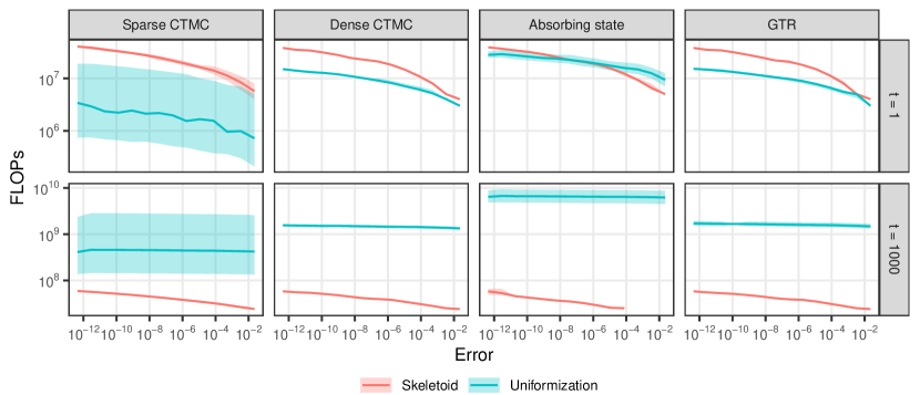
Figure 2: FLOPs associated to matrix multiplications needed to compute approximate solutions to the transition function for random rate matrices of size 100, versus the $\ell_{\infty}$ error incurred. Rows represent increasing time exponents ($t$ in $e^{tQ}$). Lines show mean error over 100 repetitions of a given combination, while bands give a 95% coverage range. The mean rate of each random rate matrix is normalized to 1.

Fig. 2 shows the performance of uniformization and skeletoid in approximating the exponential of random rate matrices $Q$ drawn at random from four qualitatively different classes of CTMCs. In the sparse class, for each row we sample a random integer giving the number of non-zero entries, and then sample the positions of these elements in each row at random. In contrast, matrices in the dense clase have only non-zero entries. In the absorbing state class we make the first state absorbing, meaning that $q_{1j}=0$ for all $j$; then, we draw a random dense rate sub-matrix for the remaining states, and finally complete the first column to satisfy the conservative property. Lastly, in the General Time Reversible (GTR) class we simulate matrices satisfying detailed balance: $\mu_{x}q_{x,y}=\mu_{y}q_{y,x}$ for all $x,y$, for some probability vector $\mu$. In all these classes, the non-zero off-diagonal elements of the matrices are drawn from $\mathrm{Exp}(1)$ distributions; then, the diagonal is set to enforce the conservative property, and finally the matrix is scaled to achieve a mean rate of one. Note that the skeletoid is much faster than uniformization in the $t=1000$ setting, across all four CTMC classes, whereas in the $t=1$ setting, the ranking of the two methods depend on the computational budget.

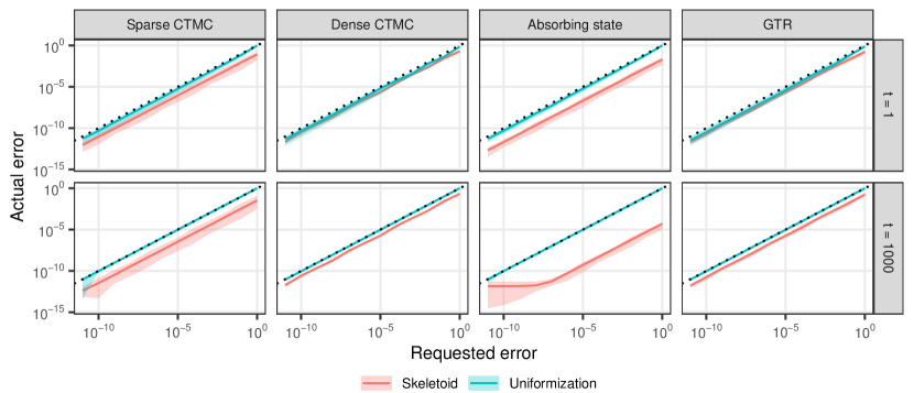
Figure 3: Realized $\ell_{\infty}$ error versus requested error for the two algorithms when applied to random rate matrices of size 100. Rows represent increasing time exponents ($t$ in $e^{tQ}$). Lines show mean error over 100 repetitions of a given combination, while bands denote the range of the error. The dotted diagonal line represents ideal behavior. The mean rate of each rate matrix is normalized to 1.

Fig. 3 shows the result of using Eqs. 35 and 42 to produce approximations with a given error bound. We see a high level of agreement between requested and realized errors in most of the settings, with a bias towards more conservative outcomes when disagreement occurs.

Notwithstanding the usefulness of Eqs. 34 and 41 to provide bounds on errors that can be evaluated before doing any computation, monotone increasing approximations (not necessarily doubly monotone) to the matrix exponential of rate matrices—like skeletoid and uniformization—offer a simple way of obtaining the exact error of a given approximation, since

$$\|M(t)-M^{(s)}(t)\|_{\infty}=\sup_{x\in\mathscr{X}}\sum_{y\in\mathscr{X}}[M(t)_{x,y}-M^{(s)}(t)_{x,y}]\leq 1-\inf_{x\in\mathscr{X}}\sum_{y\in\mathscr{X}}M^{(s)}(t)_{x,y},$$

where the inequality arises from the possibility that $Q$ is non-conservative. The right-hand side is computable since the formula does not depend on $M(t)$. The inequality becomes an equality in the case of a conservative $Q$, and in this case a stronger statement holds for all $x\in\mathscr{X}$:

$$\sum_{y\in\mathscr{X}}[M(t)_{x,y}-M^{(s)}(t)_{x,y}]=1-\sum_{y\in\mathscr{X}}M^{(s)}(t)_{x,y}.$$

Finally, we note that it is always possible to improve a collection of monotone increasing approximations by computing all of them in parallel and returning their element-wise maximum, which will again be monotone increasing. However, in our tests the overhead needed to parallelize the skeletoid and uniformization methods was not compensated by the efficiency gains obtained. However, it is possible that for models not considered in this study, an algorithm returning the element-wise maximum of the uniformization, skeletoid, and potentially other monotone approximations could be advantageous.

4 Related work

Georgoulas et al. (2017) were the first to describe a pseudo-marginal method to perform exact inference for CTMCs on countably infinite spaces by debiasing a sequence of likelihood estimates arising from an increasing sequence of truncated state-spaces. They used the randomly-truncated series debiasing scheme first introduced by McLeish (2011), which has the downside of requiring an unbounded random number of calls to the matrix exponentiation algorithm. In contrast, the OSTE scheme needs at most $3$ calls to these routines. Additionally, Georgoulas et al. (2017) used a stopping time whose distribution has super-exponential tails. This introduces the risk of obtaining likelihood estimates with infinite variance, unless one is able to prove that the approximating sequence converges faster. As discussed in Section 3.2, there is evidence that the sequences converge at super-exponential speed, but the precise rate must still be estimated on a case-by-case basis.

Building on Georgoulas et al. (2017), Sherlock and Golightly (2019) introduced the MESA algorithm. This method expands the state space of the sampler to include the random index $r$ of the smallest truncated state space that contains the full (unobserved) path of the process for all observation pairs. This strategy is appealing because it dispenses with the need to design debiasing methods with appropriate stopping times. The variant nMESA is also proposed, which has a different index $r_{i}$ for each observation pair. In terms of computational cost, the sampler used in MESA requires $3$ calls to matrix exponentiation routines, which are based on uniformization and scaling-and-squaring. On the other hand, because they are not pseudo-marginal samplers, neither MESA nor nMESA can take advantage of the accuracy relaxation technique described in Section 3.4. Thus, they require computing matrix exponentials up to numerical accuracy.

Previous work has explored the use of particle MCMC to design positive unbiased estimators in the context of infinite state space CTMC. The most straightforward way to use particle MCMC for infinite CTMC is to impute full paths and set weights to zero when a particle does not match an observed end-point (Saeedi and Bouchard-Côté, 2011; Golightly and Wilkinson, 2011). However this approach can suffer from severe weight degeneracy, including particle population collapse where all weights are equal to zero. A more sophisticated approach builds a martingale to guide particle paths toward the end-point (Hajiaghayi et al., 2014), but this requires the construction of a problem-specific potential function.

The literature on exact inference for CTMCs on finite state spaces is extensive (see e.g. Geweke et al., 1986; Fearnhead and Sherlock, 2006; Ferreira and Suchard, 2008), but methods therein cannot be extended to the countably infinite case in a straightforward manner. In particular, as we have previously mentioned, uniformization cannot be applied to infinite state-space CTMCs whose rate matrices do not admit a uniform bound on the diagonal. Another line of work has built advanced extensions for the related but distinct problem of end-point simulation (Rao and Teh, 2013; Zhang and Rao, 2020).

5 Experiments

input : $n_{\text{samples}},\theta_{0},\Sigma_{\text{prop}},p,\{r(n),k(n)\}_{n\in{\mathbb{Z}}_{+}}$

$\mathcal{C}\leftarrow\{\mathscr{X}_{0}\}$

  $\triangleright$ construct and store $\mathscr{X}_{0}$

$\bar{r}\leftarrow 0$

  $\triangleright$ index of the largest state-space available

$N\sim\text{Geom}(p)$

$L_{\text{cur}}\leftarrow\tilde{L}_{\text{RA}}(\theta_{0},N)$

  $\triangleright$ using Eq. 30 with $\{r(n),k(n)\}_{n\in{\mathbb{Z}}_{+}}$

for $s=1,2,\dots,n_{\text{samples}}-1$ do

       $\theta_{\text{prop}}|\theta_{s-1}\sim\mathcal{N}(\theta,\Sigma_{\text{prop}})$

       $N\sim\text{Geom}(p)$

       if $r(N+1)>\bar{r}$ then $\triangleright$ need to build larger state-spaces

             $\mathcal{C}\leftarrow\mathcal{C}\cup\{\mathscr{X}_{r}\}$ for all $r\in\{\bar{r}+1,\dots,r(N+1)\}$

             $\bar{r}\leftarrow r(N+1)$

            

       end if

      $L_{\text{prop}}\leftarrow\tilde{L}_{\text{RA}}(\theta_{\text{prop}},N)$

       $A\leftarrow 1\wedge\frac{\pi(\theta_{\text{prop}})L_{\text{prop}}}{\pi(\theta_{s-1})L_{\text{cur}}}$

       $U\sim U[0,1]$

       if $U\leq A$ then $\triangleright$ proposal accepted

             $\theta_{s}\leftarrow\theta_{\text{prop}}$

             $L_{\text{cur}}\leftarrow L_{\text{prop}}$

            

       else  $\triangleright$ proposal rejected

             $\theta_{s}\leftarrow\theta_{s-1}$

            

       end if

      

end for

output : $\{\theta_{s}\}_{s=0}^{n_{\text{samples}}-1}$.

Algorithm 2 Metropolis pseudo-marginal sampler with RA estimator

We evaluate our methods using experimental benchmarks introduced in Georgoulas et al. (2017) and Sherlock and Golightly (2019). We run a random walk Metropolis sampler targeting the augmented posterior distribution $\pi(\theta,U|\mathcal{D})$ of Eq. 7. The proposal for $\theta$ uses a multivariate normal with covariance matrix $\Sigma_{\text{prop}}=\alpha\operatorname{Var}(\theta|\mathcal{D})$, for some $\alpha>0$ and with $\operatorname{Var}(\theta|\mathcal{D})$ estimated in a trial run. For the auxiliary variables $U$ we take independent draws from the distribution used by the OSTE scheme, which we set to $\text{Geom}(p)$ distributions with $p\in(0,1)$. Section A.5 contains detailed explanations on how to tune all the parameters involved. An overview of the process to run the Metropolis sampler using the RA estimator is shown in Algorithm 2. The process used for a sampler using the IA estimator is similar but involves also looping over observations.

In order to fairly compare the efficiency of algorithms implemented in different languages, we use the effective sample size per billion floating point operations (ESS/GFLOPs), when considering FLOPs used in matrix multiplications within matrix exponentiation algorithms. The reason to focus on these operations is that they account for most of the computational cost incurred by the samplers. The ESS is measured using the method implemented in the R package mcmcse (Flegal et al., 2020) and described by Gong and Flegal (2016). Due to the importance of correctly tuning samplers to obtain good results, we only compare against other methods that have been previously tuned for and tested in a given dataset by their respective authors.

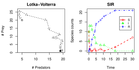
Figure 4: Plots of the datasets considered in the experiments. Dashed lines are used to emphasize that the path of the process is unknown between observations. Top: datasets from Sherlock and Golightly (2019) for the Lotka–Volterra (3 reactions) and Schlögl models. Bottom: datasets from Georgoulas et al. (2017) for the Lotka–Volterra (4 reactions) and SIR models

5.1 Schlögl model

The Schlögl model is defined by four reactions

$$\begin{array}[]{ccc}A+2X&\xrightarrow{\mathmakebox[7em]{\theta_{1}X(X-1)/2}}&3X\\ 3X&\xrightarrow{\theta_{2}X(X-1)(X-2)/6}&2X+A\\ B&\xrightarrow{\mathmakebox[7em]{\theta_{3}}}&X\\ X&\xrightarrow{\mathmakebox[7em]{\theta_{4}X}}&B\\ \end{array}$$ (43)

where the number of $A$ and $B$ molecules are kept constant, so that the only species evolving in time is $X$. The model is known in the mathematical biology literature as the canonical example of a chemical reaction system exhibiting “bi-stability” (Vellela and Qian, 2009). This means that for some parameter configurations, the system oscillates between two meta-states or regimes, one with very low or zero counts of $X$, and one with high counts.

For the purpose of inference, it is simpler to work with the birth–death version of the process, obtained by collapsing the reactions that increase $X$ and the ones that decrease it

$$\lambda_{x} =\theta_{1}{\mathbf{1}}\{x\geq 2\}x(x-1)/2+\theta_{3}$$ (44)

$$\mu_{x} =\theta_{2}{\mathbf{1}}\{x\geq 3\}x(x-1)(x-2)/6+{\mathbf{1}}\{x\geq 1\}\theta_{4}$$ (45)

for $x\in{\mathbb{Z}}_{+}$.

Figure 5: Trace plots for 10,000 samples taken using 3 parallel chains of the RA pseudo-marginal sampler with Skeletoid targeting the posterior distribution of the Schlögl model.

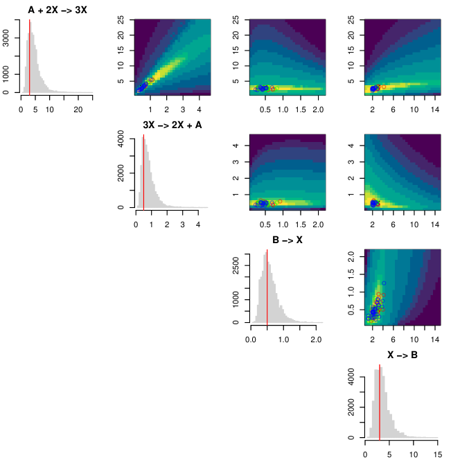
Figure 6: Histograms of the samples obtained from the experiment described in Fig. 5. Heatmaps show bi-variate views of the approximated posterior when using the approximate likelihood $L_{r}^{k}$ (Eq. 28) with high values of $r,k$. Vertical lines in histograms and X’s in bi-variate plots show location of data-generating parameter. Points in bi-variate plots show selected samples from every chain.

To give a more detailed description of the performance of our pseudo-marginal approach, we first focus on the results obtained for the Schlögl model, then present summaries for several models. The dataset we use is taken from Sherlock and Golightly (2019), and is depicted in Fig. 4. Note that it exhibits the bi-stability phenomenon described above. These data are taken every $\Delta t=4$ from a path simulated with $\theta_{\text{true}}=(3,0.5,0.5,3)$. Sherlock and Golightly (2019) use a Metropolis sampler on the log-transformed variables $\xi=\log(\theta)$, and place independent standard normal priors on $\xi$. Since we work directly with $\theta$, we use i.i.d. standard log-normals. After following the tuning procedure outlined in Section A.5, we run three parallel chains for 10,000 iterations each, initialized at $\theta_{\text{true}}$. Fig. 5 shows the trace-plots for an RA sampler using the skeletoid method, evidencing good mixing in all parameters and chains. Fig. 6 summarizes the approximated posterior. Note how there is almost perfect correlation between $\theta_{1}$ and $\theta_{2}$, demonstrating that having a proposal with non-diagonal covariance is useful.

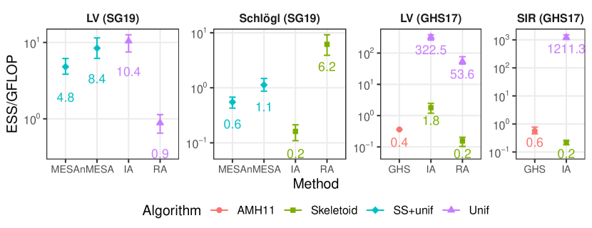
Figure 7: Comparison of ESS/GFLOP between our proposed pseudo-marginal samplers and competing methods. The intervals denote the range across 30 repetitions, while points and text correspond to the means.

The second panel in Fig. 7 shows the ESS/GFLOP achieved by the IA and RA samplers with the skeletoid, compared to the results obtained for the MESA and nMESA methods. Our RA sampler achieves an improvement of more than 450% over nMESA.

5.2 Lotka–Volterra model

The Lotka–Volterra (LV) LV process has state-space $\mathscr{X}={\mathbb{Z}}_{+}^{2}$; i.e., defined by boundaries $B^{l}=(0,0)$ and $B^{u}=(\infty,\infty)$. We consider two versions of this model with different numbers of reactions.

5.2.1 Three reactions

Sherlock and Golightly (2019) use a version of LV containing three distinct reactions

$$\begin{array}[]{cccl}R&\xrightarrow{\mathmakebox[2em]{\theta_{1}R}}&\emptyset&\text{(death of predator)}\\ R+Y&\xrightarrow{\theta_{2}RY}&2R&\text{(predator eats prey \& reproduces)}\\ Y&\xrightarrow{\mathmakebox[2em]{\theta_{3}Y}}&2Y&\text{(birth of prey)}\end{array}$$ (46)

Here, $R$ denotes the number of predators and $Y$ the size of the prey population. For our experiments, we focus on the LV20 dataset—shown in the top-left panel of Fig. 4—containing 20 observations obtained at regular time intervals $\Delta t=1$ of an LV path simulated with $\theta_{\text{true}}=(0.3,0.4,0.01)$. Again, Sherlock and Golightly (2019) use a Metropolis sampler on the log-transformed variables $\xi$, putting independent Gaussian priors with unit variance and means $(\log(0.2),\log(0.2),\log(0.02))$. To match these, we put independent log-normal priors on $\theta$ with the same parameters.

In the first panel of Fig. 7 we show that the IA sampler with uniformization achieves more than a 20% average increase in ESS/GFLOP when compared agains nMESA, although the ranges do not show a strong separation. These results also show that the relative performance between IA and RA samplers depends on the particulars of the model and data.

5.2.2 Four reactions

Georgoulas et al. (2017) use a version of the LV model with four reactions

$$\begin{array}[]{cccl}R&\xrightarrow{\mathmakebox[2em]{\theta_{1}R}}&\emptyset&\text{(death of predator)}\\ R+Y&\xrightarrow{\theta_{2}RY}&2R+Y&\text{(birth of predator)}\\ R+Y&\xrightarrow{\theta_{3}RY}&R&\text{(death of prey)}\\ Y&\xrightarrow{\mathmakebox[2em]{\theta_{4}Y}}&2Y&\text{(birth of prey)}\end{array}$$ (47)

The data used by the authors is depicted in the bottom-left panel of Fig. 4. It represents observations at regular intervals with $\Delta t=200$ of a path simulated using $\theta_{\text{true}}=(1,5,5,1)\cdot 10^{-4}$.

We compare our methods against the pseudo-marginal sampler proposed by the authors, which builds a chain directly targeting the augmented posterior for $\theta$ using i.i.d. $\text{Gamma}(4,10^{4})$ priors. As the third panel in Fig. 7 shows, we achieve an improvement of 3 orders of magnitude using the IA sampler with uniformization. AMH11 denotes the matrix exponentiation algorithm described in Al-Mohy and Higham (2011).

5.3 SSIR model

The last CTMC we consider is the SSIR model, described in detail in Section 2.2. The data—taken from Georgoulas et al. (2017) and shown in the bottom-right panel of Fig. 4—are obtained from observations taken at irregular time steps from a path simulated using $\theta_{\text{true}}=(0.4,0.5,0.4)$. In our experiments, we match the prior used by the authors, corresponding to i.i.d. $\text{Gamma}(1.5,5)$. We can see in the last panel of Fig. 7 that the IA sampler with uniformization achieves an improvement of almost 4 orders of magnitude.

6 Conclusions

In this work we have proposed pseudo-marginal methods based on monotonic approximations to the likelihood of stochastic processes with intractable transition functions. A monotonic approximation can be seen as one of two inputs—the other being a debiasing scheme—of an almost automatic procedure for designing pseudo-marginal samplers targeting the correct posterior distribution. To this end, we have described the OSTE scheme which improves over other debiasing methods by using a bounded number of calls to the approximating sequence, and by offering a flexible way to balance the variance-cost trade-off. We have also shown how to accelerate a recently proposed pseudo-marginal sampler for countable state-space CTMCs by considering matrix exponentiation algorithms that produce increasing approximations when applied to finite rate matrices. Moreover, we have introduced the skeletoid as a novel probabilistic approach for computing monotonic approximations to the exponential of rate matrices, that excels in cases where the norm of these matrices is high. Finally, we have given experimental evidence that our proposed algorithms offer sizable efficiency gains.

Note that the only component of the proposed algorithms that is tailored to reaction networks is the design of the increasing sequence of state-spaces. Therefore, extending our algorithms to CTMCs other than the ones considered in this study should not be cumbersome. Some interesting areas of application include CTMCs arising from the study of the secondary structure of nucleic acids through elementary step kinetic models (Schaeffer et al., 2015; Zolaktaf et al., 2019), as well as CTMCs underlying state-dependent speciation and extinction models in phylogenetics (Maddison et al., 2007; Louca and Pennell, 2019).

More generally, we aim to extend the “monotone approximation plus debiasing” framework to other stochastic processes with intractable likelihoods. For example, exact inference methods for diffusions exist only for a restricted class of such processes (Beskos et al., 2006; Sermaidis et al., 2013). On the other hand, there is a growing literature on asymptotic expansions to the transition functions of diffusions (Aït-Sahalia et al., 2008; Li et al., 2013) which are valid in more general settings. These expansions could potentially be modified to produce monotone approximations, thus enabling the use of our framework for exact inference. A different way to tackle this problem would be to rely on techniques to approximate diffusions using CTMCs (Kushner, 1980; Di Masi and Runggaldier, 1981). As long as the transition function of the latter converges monotonically to the transition function of the diffusion, the methods in this paper could be applied.

Appendix A Implementation details

A.1 Numerically stable implementation of the skeletoid method

When $\delta=t2^{-k}$ is close to the machine’s precision, the straightforward computation of $S(t2^{-k})^{2^{k}}$ produces rounding errors. The reason is that in these cases $S(\delta)\approx I$. A simple way to bypass this issue is to rely on the identity

$$A^{2}=(I+A-I)^{2}=I+2(A-I)+(A-I)^{2}$$

which holds for any square matrix $A$. Defining $B:=A-I$, the identity becomes

$$A^{2}=I+B^{\prime}\hskip 10.00002pt\text{with}\hskip 10.00002ptB^{\prime}=2B+B^{2}$$

An inductive argument then shows that we can compute $A^{2^{k}}$ via the recursion depicted in Algorithm 3.

input : $B:=A-I,k$

for $i=1,2,\dots,k$ do  $B\leftarrow 2B+B^{2}$

output : $A^{2^{k}}=I+B$.

Algorithm 3 Implicit matrix squaring

To fully take advantage of Algorithm 3 we must implicitly compute $S(\delta)-I$. This is achieved by replacing the formula for the diagonal elements in Eq. 37 by

$$[S(\delta)]_{i,i}=\mathtt{expm1}(q_{i,i}\delta)$$

where expm1 is the standard numerical routine for accurately computing $e^{x}-1$ when $x\approx 0$.

A.2 Computing elements of the matrix exponential

When computing the likelihood function we are generally interested in only a handful of entries of the transition function. This can be used to speed-up computation, by only performing computation for the rows of the matrix exponential that contain those entries.

Let $Q_{r}$ be the rate matrix associated to $\mathscr{X}_{r}$, and define $b_{r}:=|\mathscr{X}_{r}|$. Suppose we are interested in the entries $\{(i_{l},j_{l})\}_{l=1}^{m}$ of the $s$-th approximation to the transition function $M^{(s)}(t)$, with $m\ll b_{r}$. Define the matrix $L$ of size $m\times b_{r}$

$$L_{u,v}:=\left\{\begin{array}[]{cc}1&\text{if }v=j_{u},\\ 0&\text{otherwise.}\end{array}\right.$$

In the case of uniformization, recall that $P:=I-Q_{r}/\bar{q}$. Then

$$(M^{(s)}(t))_{i_{l},j_{l}}=(LM^{(s)}(t))_{l,j_{l}}=\sum_{n=0}^{s}e^{\bar{q}t}\frac{(-\bar{q}t)^{n}}{n!}(LP^{n})_{l,j_{l}}$$

Note that the matrix $LP^{n}$ can be efficiently computed recursively setting $LP^{0}=L$ and updating via $LP^{n}=(LP^{n-1})P$. Suppose that $P$ has $\eta$ non-zero elements per column on average. Then the update operation involves $\eta b_{r}$ FLOPs, so we can obtain $(M^{(s)}(t))_{i,j}$ using only $s\eta b_{r}$ operations. Compare to $s\eta b_{r}^{2}$ which would be the cost of computing the full matrix exponential.

For the skeletoid method, we can apply a trick used for computing the action of the matrix exponential obtained through scaling and squaring (Sherlock, 2018). Consider the squaring decomposition

$$S(\delta)^{2^{k}}=\underbrace{S(\delta)^{2^{k_{1}}}\cdot\dots\cdot S(\delta)^{2^{k_{1}}}}_{2^{k_{2}}\text{ times}}=\prod_{i=1}^{2^{k_{2}}}S(\delta)^{2^{k_{1}}}$$

for any $k_{1},k_{2}\in{\mathbb{Z}}_{+}$ such that $k_{1}+k_{2}=k$. Pre-multiplying by $L$

$$LS(\delta)^{2^{k}}=L\prod_{i=1}^{2^{k_{2}}}S(\delta)^{2^{k_{1}}}=(LS(\delta)^{2^{k_{1}}})\prod_{i=1}^{2^{k_{2}}-1}S(\delta)^{2^{k_{1}}}$$

Now, in general $S(\delta)^{2^{k_{1}}}$ is a dense matrix of size $b_{r}\times b_{r}$ (due to CTMCs being irreducible in general), so we model its computational cost to $k_{1}b_{r}^{3}$ (ignoring subcubic algorithms due to their higher associated constants for simplicity). Then the product $LS(\delta)^{2^{k_{1}}}$ costs $mb_{r}^{2}$, and so does every subsequent multiplication by $S(\delta)^{2^{k_{1}}}$ on the right. Therefore, the total cost becomes

$$C(k_{1},k_{2})=\beta k_{1}b_{r}^{3}+mb_{r}^{2}2^{k_{2}}$$

where we have added the parameter $\beta<1$ to account for the fact that $n$ vector-matrix multiplications with cost $n^{2}$ are slower than one matrix-matrix multiplication with cost $n^{3}$. We have found $\beta=0.1$ gives consistent results.

We can easily optimize the function above if we work in ${\mathbb{R}}$ by setting $x\leftarrow k_{2}$, and $k_{1}=k-x$. Indeed, let

$$C(x)=\beta(k-x)b_{r}^{3}+mb_{r}^{2}2^{x}.$$

Differentiating gives the condition

$$0=C^{\prime}(x)=-\beta b_{r}^{3}+\log(2)mb_{r}^{2}2^{x}.$$

Thus

$$x^{*}=\log_{2}\left(\frac{\beta b_{r}}{\log(2)m}\right).$$

Constraining $x^{*}$ to an integer in the correct interval gives

$$k_{2}^{*}=0\vee(k\wedge\arg\min\{C(y):y\in\{\lfloor x^{*}\rfloor,\lceil x^{*}\rceil\}\}).$$

Finally, setting $k_{1}^{*}=k-k_{2}^{*}$ yields a strategy for computing $LS(\delta)^{2^{k}}$ which is in general faster than the naive approach requiring forming $S(\delta)^{2^{k}}$.

A.3 Building the base state space

Here we present a heuristic for computing a “seed” path between pairs of observations that is specialized to reaction networks with $\mathscr{X}={\mathbb{Z}}_{+}^{n_{s}}$. Fix an observed change in the state of the system $(x_{i-1},x_{i},\Delta t_{i})$, with $\Delta t_{i}:=t_{i}-t_{i-1}$. Assuming non-explosivity, there exists a finite sequence of states $\{s_{p}\}_{p=0}^{P}$ and a corresponding sequence of reactions $\{r_{p}\}_{p=1}^{P}$—with $s_{0}=x_{i-1}$ and $s_{P}=x_{i}$—such that for all $p\in\{1,\dots,P\}$

$$s_{p}=s_{p-1}+U_{r_{p},\cdot},$$

where $U$ is the reaction matrix of the model of size $n_{r}\times n_{s}$. Unrolling the above recursion yields

$$\Delta x_{i}:=x_{i}-x_{i-1}=\sum_{p=1}^{P}U_{r_{p},\cdot}=U^{T}\nu,$$ (48)

where $\nu\in{\mathbb{Z}}_{+}^{n_{r}}$ is an integer vector denoting the number of times each reaction is used to form the path.

The solution to Eq. 48, although not necessarily unique, can be computed by expressing the problem as an Integer Program

$$\begin{array}[]{ccc}\displaystyle\min_{\nu\in{\mathbb{Z}}^{n_{r}}}\boldsymbol{1}_{n_{r}}^{T}\nu&\text{s.t.}&U^{T}\nu=\Delta x_{i},\;\nu\geq 0.\end{array}$$

Since for the reaction networks considered in this paper, $n_{r},n_{s}<10$, the problem is computationally tractable. Moreover, since $\Delta x_{i}$ is an integer vector, when $U$ is Totally Unimodular—which is the case for all the reaction networks we experiment with—the corresponding Linear Program relaxation yields an integer solution (Hoffman and Kruskal, 1956). Finally, once $\nu$ is obtained, we recover the path $\{s_{p}\}_{p=1}^{P}$—with $P:=\boldsymbol{1}_{n_{r}}^{T}\nu$—using a simple heuristic search algorithm.

A.4 Numerically stable computation of the log-likelihood

The formula for computing $\tilde{L}_{\text{RA}}(\theta,U)$ in Eq. 30 is numerically unstable because it depends on the products in Eq. 28, which in most cases will be $\approx 0$. However, we can use the following identities to directly compute $\log(\tilde{L}_{\text{RA}}(\theta,U))$ without explicitly computing products. The function expm1 is the standard numerical routine for accurately computing $e^{x}-1$ when $x\approx 0$. Similarly, log1p refers to standard numerical routines that accurately compute $\log(1+x)$ for $|x|\ll 1$.

Proposition 11.

Let $0\leq p_{1}\leq p_{2}\leq p_{3}$. Fix $\alpha\in(0,1]$ and let

$$z:=p_{1}+\frac{p_{3}-p_{2}}{\alpha}.$$

Define $s_{i}:=\log(p_{i})$ for each $i\in\{1,2,3\}$. Then

$$\log(z)=\left\{\begin{array}[]{cc}-\infty&p_{3}=0\\ s_{3}-\log(\alpha)&p_{3}>0,p_{2}=0\\ s_{2}+\log(\mathtt{expm1}(s_{3}-s_{2}))-\log(\alpha)&p_{2}>0,p_{1}=0\\ s_{1}+\mathtt{log1p}\left(\exp(s_{2}-s_{1}-\log(\alpha))\mathtt{expm1}(s_{3}-s_{2})\right)&\text{otherwise.}\end{array}\right.$$ (53)

Proof.

The first two cases follow directly. For the third case, note that

$$z=\frac{\exp(s_{3})-\exp(s_{2})}{\alpha}=\exp(s_{2})\frac{(\exp(s_{3}-s_{2})-1)}{\alpha}=\exp(s_{2})\frac{\mathtt{expm1}(s_{3}-s_{2})}{\alpha}.$$

Hence

$$\log(z)=s_{2}+\log(\mathtt{expm1}(s_{3}-s_{2}))-\log(\alpha).$$

The general case follows similarly

$$z =\exp(s_{1})+\frac{\exp(s_{3})-\exp(s_{2})}{\alpha}$$ (54)

$$=\exp(s_{1})\left(1+\frac{\exp(s_{3})-\exp(s_{2})}{\alpha\exp(s_{1})}\right)$$ (55)

$$=\exp(s_{1})\left(1+\exp(s_{2})\frac{\mathtt{expm1}(s_{3}-s_{2})}{\alpha\exp(s_{1})}\right)$$ (56)

$$=\exp(s_{1})\left(1+\exp(s_{2}-s_{1}-\log(\alpha))\mathtt{expm1}(s_{3}-s_{2})\right).$$ (57)

Taking $\log(\cdot)$ at both sides gives the required expression

$$\log(z)=s_{1}+\mathtt{log1p}(\exp(s_{2}-s_{1}-\log(\alpha))\mathtt{expm1}(s_{3}-s_{2})).$$

∎

A.5 Tuning the pseudo-marginal samplers

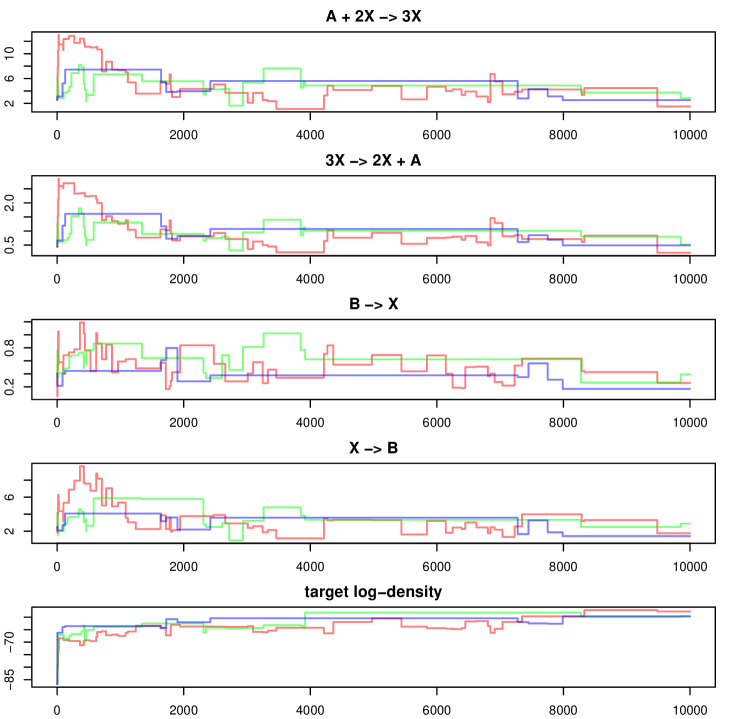
Figure 8: Example of a poorly tuned pseudo-marginal sampler for the Schlögl model. Each line depicts an independent parallel chain.

The approach we have presented depends crucially on correctly tuning the joint truncation–accuracy sequences (see Section 3.4) and the probability mass function $p(n)$ of the stopping times so that de-biasing behaves properly. As Fig. 8 shows, without proper tuning the sampler can give rise to chains that get stuck for long stretches (in stark contrast to Fig. 5). The reason for this behavior is to be found in Eq. 10. The ratio can give rise to arbitrarily high estimates of the likelihood if the probability mass function $p(n)$ is much smaller than the observed decrease in error (i.e., the numerator). In this respect, the design of $p(n)$ bears similarity with the design of proposal distributions for importance sampling, as we must ensure that the tails of $p(n)$ match the decay of the first differences $a_{\omega+n+1}-a_{\omega+n}$.

There is a growing literature concerned with optimally tuning pseudo-marginal samplers to maximize some measure of efficiency (Pitt et al., 2012; Doucet et al., 2015; Sherlock et al., 2015; Schmon et al., 2020). Recall the augmented target density in Eq. 7, and define

$$\zeta(\theta,U):=\log(\tilde{L}(\theta,U))-\log(L(\theta)).$$ (58)

Moreover, let $\sigma_{\zeta}^{2}(\theta):=\operatorname{Var}(\zeta|\theta)$. The recommendations suggest tuning the sampler to achieve $\sigma_{\zeta}(\theta_{\text{MAP}})=\bar{\sigma}$, for some pre-specified target $\bar{\sigma}$, and with $\theta_{\text{MAP}}$ a mode of $\pi(\theta|\mathcal{D})$. The benefit of this approach is that it does not require running the chains for long periods of time with different configurations, since $\sigma_{\zeta}(\theta_{\text{MAP}})$ can be estimated using simple Monte Carlo whenever we can sample $U\sim m$.

On the other hand, depending on the particular assumptions of each study, the recommended $\bar{\sigma}$ ranges from 0.92 to 1.8. Given the ambiguity of these different recommendations, we use $\sigma_{\zeta}(\theta_{\text{MAP}})$ not as something to tune in itself, but as a summary of the characteristics of different samplers. In short, we tune our samplers following these steps:

1. Tune a sampler with a default value of $p_{\text{min}}=0.9$ (as shown in the next paragraphs) and do a preliminary run to find $\theta_{\text{MAP}}$ and an estimate $\widehat{\operatorname{Var}}(\theta|\mathcal{D})$ of $\operatorname{Var}(\theta|\mathcal{D})$.

2. Design an array of different samplers by running the tuning procedure explained in the next paragraphs for all

   $$p_{\text{min}}\in\{0,0.01,0.1,0.2,0.4,0.6,0.8,0.9\}$$

3. For each sampler, take $\{U_{i}\}_{i=1}^{100}\stackrel{{\scriptstyle\scriptscriptstyle\textrm{iid}}}{{\sim}}m$ and estimate $\sigma_{\zeta}(\theta_{\text{MAP}})$ using simple Monte Carlo. Also, record the time needed to compute that estimate

4. For each $\bar{\sigma}\in\{0.1,1,1.5,2\}$, find the sampler giving $\sigma_{\zeta}(\theta_{\text{MAP}})\leq\bar{\sigma}$ in the shortest time.

5. For each sampler in this shortlist

   1. Optimize $\alpha$ in the variance of the proposal $\Sigma=\alpha\widehat{\operatorname{Var}}(\theta|\mathcal{D})$, aiming to maximize ESS per compute time, using a grid search.

   2. Run the sampler with the tuned variance for a longer time and get an estimate of ESS per compute time.

6. Select the sampler giving the highest ESS per compute time.

To implement the general outline described above, let us assume that for every observation $i\in\{1,\dots,n_{d}\}$ and every $r\in{\mathbb{Z}}_{+}$, the sequence $\{M_{r}^{(k)}(\Delta t_{i})_{x_{i-1},x_{i}}\}_{k\in{\mathbb{Z}}_{+}}$ satisfies a specific version of the second condition in Eq. 24 (Proposition 5), namely

$$M_{r}(\Delta t_{i})_{x_{i-1},x_{i}}-M_{r}^{(k)}(\Delta t_{i})_{x_{i-1},x_{i}}\leq 10^{-k}.$$ (59)

Note that we can always satisfy Eq. 59 through the use of Eq. 35 or Eq. 42 (depending on the algorithm). Moreover, since Eq. 59 works for $k\in{\mathbb{R}}_{+}$ too, we re-index the collection of approximate transition probabilities with $\{M_{r}^{(k)}(\Delta t_{i})_{x_{i-1},x_{i}}\}_{r\in{\mathbb{Z}}_{+},k\in{\mathbb{R}}_{+}}$. This allows us to have a finer control in the tuning process.

In order to have a generic tuning procedure that works for both IA and RA estimators, let $a_{r}^{(k)}$ be either

• the estimated transition probability for the $i$-th observation $M_{r}^{(k)}(\Delta t_{i})_{x_{i-1},x_{i}}$, if using method IA (see Eq. 26), or

• the estimated likelihood for the full data $L_{r}^{(k)}(\theta)$ if using method RA (see Eq. 28).

Following the conclusions of Proposition 5, we parametrize the sequence of pairs $\{(r_{n},k_{n})\}_{n\in{\mathbb{Z}}_{+}}$ using a simple linear form

$$\forall n\in{\mathbb{Z}}_{+}:r_{n}:=\omega^{(\text{T})}+n\qquad\text{ and }\qquad k_{n}:=\omega^{(\text{S})}+\sigma n,$$ (60)

where $\omega^{(\text{T})}\in{\mathbb{Z}}_{+}$ is a truncation offset, $\omega^{(\text{S})}\in{\mathbb{R}}$ an approximation quality offset, and $\sigma>0$ a relative step-size. Indeed, in Proposition 5, the offsets are $0$ and $\sigma=\rho/\kappa$ if one allows for $k_{n}\in{\mathbb{R}}_{+}$ as we do here. We shall see that having non-zero offsets lets us control de variance of the estimators.

Let us begin by setting $\omega^{(\text{T})},\omega^{(\text{S})}$ to preliminary values. Define

$$a_{r}^{(\infty)} :=\lim_{k\to\infty}a_{r}^{(k)}\hskip 10.00002pt\forall r\in{\mathbb{Z}}_{+}$$ (61)

$$a_{\infty}^{(k)} :=\lim_{r\to\infty}a_{r}^{(k)}\hskip 10.00002pt\forall k\in{\mathbb{R}}_{+}$$ (62)

$$\alpha :=\lim_{r\to\infty}a_{r}^{(\infty)}$$ (63)

$\alpha$ denotes the target quantity to be estimated; that is, either the transition probability $M(\Delta t_{i})_{x_{i-1},x_{i}}$ if using the IA method, or the likelihood $L(\theta)$ if using the RA approach. Proposition 1 shows that we can arbitrarily reduce the variance of $Z$ by increasing the offset $\omega$. On the other hand, the cost of computing $Z$ is at least the cost of computing $a_{\omega}$, which in our context increases to $\infty$ as $\omega\to\infty$. It follows that there should be a sweet-spot maximizing the efficiency of the sampler. Following this intuition, we would set

$$\omega^{(\text{T})} =\min\left\{r\in{\mathbb{Z}}_{+}:a_{r}^{(\infty)}\geq p_{\text{min}}\alpha\right\}$$ (64)

$$\omega^{(\text{S})} =\min\left\{k\in{\mathbb{R}}_{+}:a_{\infty}^{(k)}\geq p_{\text{min}}\alpha\right\}$$ (65)

for some $p_{\text{min}}\in(0,1)$ which would reflect a trade-off between guaranteed accuracy and cost. In turn, $p_{\text{min}}$ would be set by maximizing ESS per compute time.

input : $\epsilon=10^{-8},r_{\text{explore}}=15$

Set accuracy $k_{\epsilon}$ to achieve error $\epsilon$ using Eq. 35 or Eq. 42

$\triangleright$ Step 1: analyze truncation $r$ at fixed algorithm setting $k=k_{\epsilon}$

$D^{(\text{T})}\leftarrow\emptyset$

  $\triangleright$ storage for truncation profile

$a_{\text{old}}\leftarrow 0,\Delta\leftarrow\infty,r\leftarrow 0$

while $r<r_{\text{ explore}}$ or $\Delta\geq\epsilon$ do

       $a_{\text{new}}\leftarrow a_{r}^{k_{\epsilon}}$

        $\triangleright$ get estimate at $(r,k_{\epsilon})$ accuracy

       $D^{(\text{T})}\leftarrow D^{(\text{T})}\cup\{[r,a_{\text{new}}]\}$

        $\triangleright$ add to profile

       $\Delta\leftarrow a_{\text{new}}-a_{\text{old}}$

       $a_{\text{old}}\leftarrow a_{\text{new}}$

       $r\leftarrow r+1$

      

end while

$r_{\epsilon}\leftarrow r-1$

  $\triangleright$ truncation achieving $\Delta<\epsilon$

$a^{*}\leftarrow a_{\text{new}}$

  $\triangleright$ best guess of exact solution

$\triangleright$ Step 2: analyze algorithm setting $k$ at fixed truncation $r=r_{\epsilon}$.

$D^{(\text{S})}\leftarrow\emptyset$

  $\triangleright$ storage for accuracy profile

$\Delta\leftarrow 1,k\leftarrow-10$

while $\Delta\geq\epsilon$ do

       $a_{\text{new}}\leftarrow a_{r_{\epsilon}}^{k}$

        $\triangleright$ get estimate at $(r_{\epsilon},k)$ accuracy

       $D^{(\text{S})}\leftarrow D^{(\text{S})}\cup\{[k,a_{\text{new}}]\}$

        $\triangleright$ add to profile

       $\Delta\leftarrow a^{*}-a_{\text{new}}$

       $k\leftarrow k+1$

      

end while

$k_{\epsilon}\leftarrow k-1$

  $\triangleright$ algorithm setting achieving $\Delta<\epsilon$

output : $D^{(\text{T})},D^{(\text{S})},a^{*},r_{\epsilon},k_{\epsilon}$

Algorithm 4 Separate analysis of convergence of sequences

Implementing the above strategy has the obvious drawback that $\alpha$ is unknown. Moreover, we do not have a theoretical bound for the truncation error that would tell us how high to set $r$ to approximate $\alpha$. A similar thing happens with the matrix exponential approximation error when we use the skeletoid method, since its bound can be loose in some settings. We must therefore begin by empirically inspecting the behavior of $\{a_{r}^{\infty}\}_{r\in{\mathbb{Z}}_{+}}$ and $\{a_{\infty}^{k}\}_{k\in{\mathbb{R}}_{+}}$. Algorithm 4 achieves this by first exploring the truncation sequence when the matrix exponentiation algorithm is set to a fixed high precision setting, producing a truncation index $r_{\epsilon}$ at which the difference between consecutive solutions is less than a pre-specified threshold $\epsilon>0$. It also gives a best guess for the true value $a^{*}\approx\alpha$. After this, it sets the truncation to $r_{\epsilon}$ and proceeds to check the convergence in $k$ by scanning $a_{r_{\epsilon}}^{k}$ at integer values of $k$, until it finds $k_{\epsilon}$ such that $a^{*}-a_{r_{\epsilon}}^{k_{\epsilon}}<\epsilon$. The algorithm returns all these values plus the complete profiles $D^{(\text{T})},D^{(\text{S})}$.

Figure 9: Visualization of the tuning process for an RA pseudo-marginal sampler for the Schlögl model, with $\theta=\arg\max\pi(\theta|\mathcal{D})$. First row: output of Algorithm 4. Second row: profiles of the first differences computed from that output.

The first row in Fig. 9 gives an example of the output for an RA sampler for the Schlögl model. We see that truncating at $r=20$ gives a good approximation, while the skeletoid method gives a very accurate solution for $k=0$, indicating that the associated bound is indeed loose for this problem.

The output from Algorithm 4 allows us to proceed with tuning the offsets. As mentioned in Section 5, we use stopping times with distribution $N\sim\text{Geom}(p)$; i.e., $p(n)=p(1-p)^{n}$ for all $n\in{\mathbb{Z}}_{+}$. Note that this probability mass function is exponentially decreasing with rate $\beta:=-\log(1-p)$. On the other hand, we can verify that the distribution given by

$$\forall n\in{\mathbb{Z}}_{+}:p(n):=\frac{a_{\omega+n+1}-a_{\omega+n}}{\alpha-a_{\omega+n}}\propto a_{\omega+n+1}-a_{\omega+n}$$ (66)

satisfies all the requirements in Proposition 1 and gives $\operatorname{Var}(Z)=0$. Aiming to mimic this optimal distribution using a $\text{Geom}(p)$ imposes the requirement that the sequence of first differences $\Delta a_{\omega+n}:=a_{\omega+n+1}-a_{\omega+n}$ be strictly decreasing. This is in general not true for any offset, as the second row in Fig. 9 shows. Indeed, one can observe peaks at $r_{\text{peak}}=15$ and $k_{\text{peak}}=-2$ for truncation and matrix exponential accuracy respectively. Thus, we impose that offsets be set to at least the last peak observed for the corresponding $\{\Delta a_{\omega+n}\}_{n\geq 0}$ profiles

$$\omega^{(\text{T})} =r_{\text{peak}}\vee\min\{r:(r,a_{r}^{k_{\epsilon}})\in D^{(\text{T})}\text{ and }a_{r}^{k_{\epsilon}}\geq p_{\text{min}}a^{*}\}$$ (67)

$$\omega^{(\text{S})} =k_{\text{peak}}\vee\min\{k:(k,a_{r_{\epsilon}}^{k})\in D^{(\text{S})}\text{ and }a_{r_{\epsilon}}^{k}\geq p_{\text{min}}a^{*}\}.$$

input : $r_{\epsilon},k_{\epsilon},\omega^{(\text{S})},\omega^{(\text{T})},\sigma_{\text{default}}=0.1$

$\sigma\leftarrow\sigma_{\text{default}}\vee\left(\frac{r_{\epsilon}-\omega^{(\text{T})}}{k_{\epsilon}-\omega^{(\text{S})}}\right)$

  $\triangleright$ initialize with Eq. 68

$a_{\text{old}}\leftarrow a_{\omega^{(\text{T})}}^{\omega^{(\text{S})}}$

  $\triangleright$ initialize with solution at both offsets

$n\leftarrow 0;r\leftarrow\omega^{(\text{T})};\ k\leftarrow\omega^{(\text{S})}$

  $\triangleright$ initialize sequences

while $r\leq r_{\epsilon}$ and $k\leq k_{\epsilon}$ do

       $r\leftarrow\omega^{(\text{T})}+n;\ k\leftarrow\omega^{(\text{S})}+\sigma n$

       $a_{\text{new}}\leftarrow a_{r}^{k}$

        $\triangleright$ get estimate at $(r,k)$ accuracy

       while $a_{\text{old}}>a_{\text{new}}$ and $k\leq k_{\epsilon}$ do $\triangleright$ monotonicity fails

             $\sigma\leftarrow 2\sigma$

              $\triangleright$ double $\sigma$ until monotonicity holds

             $k\leftarrow\omega^{(\text{S})}+\sigma n$

             $a_{\text{new}}\leftarrow a_{r}^{k}$

              $\triangleright$ update estimate

            

       end while

      $a_{\text{old}}\leftarrow a_{\text{new}}$

       $n\leftarrow n+1$

      

end while

output : $\sigma$

Algorithm 5 Tune $\sigma$

Having set preliminary values for $\omega^{(\text{S})},\omega^{(\text{T})}$, we proceed to set $\sigma$. Following the intuition from Proposition 5, we initialize this parameter with the rule

$$\sigma=\sigma_{\text{default}}\vee\left(\frac{r_{\epsilon}-\omega^{(\text{T})}}{k_{\epsilon}-\omega^{(\text{S})}}\right).$$ (68)

The ratio on the right-hand side corresponds to an “average relative velocity” of the convergence of the matrix exponential accuracy sequence versus the truncation sequence, while $\sigma_{\text{default}}>0$ corrects border cases. For doubly monotone sequences, there is no additional tuning required. In other cases, we must set $\sigma$ high enough to ensure monotonicity holds. The process is summarized in Algorithm 5. Whenever we encounter a failure in monotonicity $a_{r_{n+1}}^{(k_{n+1})}<a_{r_{n}}^{(k_{n})}$, we double $\sigma$ and recompute $a_{r_{n+1}}^{(k_{n+1})}$ until the condition is met.

Having set $\sigma$ we can adjust the offsets to match the behavior of the joint sequence. Let $n_{\text{peak}}$ be the index of the rightmost peak in the sequence of differences $\Delta a_{n+1}:=a_{r_{n+1}}^{(k_{n+1})}-a_{r_{n}}^{(k_{n})}$. Define

$$n_{\text{offset}}:=\min\{n\geq n_{\text{peak}}:a_{r_{n}}^{(k_{n})}\geq p_{\text{min}}a^{*}\}.$$

and update the offsets to $\omega^{(\text{T})}=r_{n_{\text{offset}}}$ and $\omega^{(\text{S})}=k_{n_{\text{offset}}}$.

Finally, to tune $p_{g}$ we fit a linear regression without intercept to

$$\log(\Delta a_{n})-\log(\Delta a_{0})=\beta_{g}n+\varepsilon_{n}$$

where $\{\epsilon_{i}\}\overset{i.i.d.}{\sim}\mathcal{N}(0,\sigma_{\epsilon}^{2})$. Then we set $p_{g}=\underline{p}\vee(\overline{p}\wedge(1-e^{\widehat{\beta_{g}}}))$, where $[\underline{p},\overline{p}]$ defines a pre-specified safe interval (we use $\underline{p}=0.4$ and $\overline{p}=0.9$).

Appendix B Proofs

Proof of Proposition 1.

The fact that $Z\geq a_{\omega}$ almost surely follows directly from the definition of $Z$ and the non-decreasing property of the sequence. Unbiasedness follows by the monotone convergence theorem:

$${\mathbb{E}}[Z] =a_{\omega}+{\mathbb{E}}\left[\sum_{n:p(n)>0}{\mathbf{1}}\{N=n\}\frac{(a_{\omega+n+1}-a_{\omega+n})}{p(n)}\right]$$ (69)

$$=a_{\omega}+\sum_{n:p(n)>0}p(n)\frac{(a_{\omega+n+1}-a_{\omega+n})}{p(n)}$$ (70)

$$=a_{\omega}+\sum_{n:p(n)>0}(a_{\omega+n+1}-a_{\omega+n})$$ (71)

$$=a_{\omega}+\sum_{n\geq 0}(a_{\omega+n+1}-a_{\omega+n}) (\text{\lx@cref{creftype~refnum}{eq:debias_estimator_assu_domination}})$$ (72)

$$=\lim_{n\to\infty}a_{n}$$ (73)

$$=\alpha.$$ (74)

Let $Y:=Z-a_{\omega}$, so that

$$Y=\frac{(a_{\omega+N+1}-a_{\omega+N})}{p(N)}=\sum_{n:p(n)>0}{\mathbf{1}}\{N=n\}\frac{(a_{\omega+n+1}-a_{\omega+n})}{p(n)}.$$

Then

$$Y^{2} =\left(\sum_{n:p(n)>0}{\mathbf{1}}\{N=n\}\frac{(a_{\omega+n+1}-a_{\omega+n})}{p(n)}\right)^{2}$$ (75)

$$=\sum_{n:p(n)>0}{\mathbf{1}}\{N=n\}\frac{(a_{\omega+n+1}-a_{\omega+n})^{2}}{p(n)^{2}}.$$ (76)

Applying expectations on both sides and using the monotone convergence theorem,

$${\mathbb{E}}[Y^{2}] ={\mathbb{E}}\left[\sum_{n:p(n)>0}{\mathbf{1}}\{N=n\}\frac{(a_{\omega+n+1}-a_{\omega+n})^{2}}{p(n)^{2}}\right]$$ (77)

$$=\sum_{n:p(n)>0}{\mathbb{P}}(N=n)\frac{(a_{\omega+n+1}-a_{\omega+n})^{2}}{p(n)^{2}}$$ (78)

$$=\sum_{n:p(n)>0}\frac{(a_{\omega+n+1}-a_{\omega+n})^{2}}{p(n)}.$$ (79)

Finally, the expression for $\operatorname{Var}(Z)$ follows from

$$\operatorname{Var}(Z) =\operatorname{Var}(Y)$$ (80)

$$={\mathbb{E}}[Y^{2}]-{\mathbb{E}}[Y]^{2}$$ (81)

$$=\sum_{n:p(n)>0}\frac{(a_{\omega+n+1}-a_{\omega+n})^{2}}{p(n)}-(\alpha-a_{\omega})^{2}.$$ (82)

If the variance is finite, then the series above is finite; the fact that $a_{\omega}\uparrow\alpha$ yields $\operatorname{Var}(Z)\to 0$ as $\omega\to\infty$. ∎

Proof of Proposition 2.

Since $p(n)>0$ for all $n\in{\mathbb{Z}}_{+}$, by Proposition 1,

$$\operatorname{Var}(Z) =\sum_{n\in{\mathbb{Z}}_{+}}\frac{(a_{\omega+n+1}-a_{\omega+n})^{2}}{p(n)}-(\alpha-a_{\omega})^{2}$$ (83)

$$\leq\sum_{n\in{\mathbb{Z}}_{+}}\frac{(a_{\omega+n+1}-a_{\omega+n})^{2}}{p(n)}$$ (84)

$$\leq\sum_{n\in{\mathbb{Z}}_{+}}\frac{c^{2}e^{-2(\omega+n)r}}{e^{-n\beta}(1-e^{-\beta})}$$ (85)

$$=\frac{c^{2}e^{-2\omega\rho}}{1-e^{-\beta}}\sum_{n\in{\mathbb{Z}}_{+}}e^{-n(2\rho-\beta)}.$$ (86)

The result follows from the geometric series formula. ∎

Proof of Proposition 4.

From the monotonicity assumptions, $a_{r_{n}}^{(k_{n})}$ converges to some limit $\beta\leq\alpha$. Suppose for the purpose of contradiction that $\beta<\alpha$.

From the definition of $a_{r}$ and the assumption $r_{n}\uparrow\infty$, we can pick $n_{0}\in{\mathbb{Z}}_{+},\epsilon>0$ such that

$$a_{r_{n_{0}}}>\beta+\epsilon.$$ (87)

Then, for $j\in{\mathbb{N}}$, iteratively pick $n_{j}>n_{j-1}$ such that $k_{n_{j}}>k_{n_{j-1}}$. This is possible using the assumption $k_{n}\uparrow\infty$. Then,

$$a_{r_{n_{0}}}^{(k_{n_{j}})}\uparrow a_{r_{n_{0}}}.$$ (88)

Since $n_{j}>n_{0}$, and $r_{n}$ is increasing, $r_{n_{j}}\geq r_{n_{0}}$, and hence

$$a_{r_{n_{j}}}^{(k_{n_{j}})}\geq a_{r_{n_{0}}}^{(k_{n_{j}})}.$$ (89)

Combining Eqs. 87, 88 and 89 yields

$$\beta=\lim_{j\to\infty}a_{r_{n_{j}}}^{(k_{n_{j}})} \geq\lim_{j\to\infty}a_{r_{n_{0}}}^{(k_{n_{j}})}=a_{r_{n_{0}}}>\beta+\epsilon,$$ (90)

which is a contradiction. We conclude that $\beta=\alpha$.

∎

Proof of Proposition 5.

Since $r_{n}\uparrow\infty$ and $k_{n}\uparrow\infty$, Proposition 4 shows that $a_{r_{n}}^{(k_{n})}\uparrow\alpha$. Moreover,

$$a_{r_{n+1}}^{(k_{n+1})}-a_{r_{n}}^{(k_{n})} \leq\alpha-a_{r_{n}}^{(k_{n})}$$ (91)

$$=(\alpha-a_{r_{n}})+(a_{r_{n}}-a_{r_{n}}^{(k_{n})})$$ (92)

$$\leq c_{1}e^{-\rho n}+c_{2}e^{-\kappa\lceil(\rho/\kappa)n\rceil}$$ (93)

$$\leq c_{1}e^{-\rho n}+c_{2}e^{-\kappa(\rho/\kappa)n}$$ (94)

$$\leq 2\max\{c_{1},c_{2}\}e^{-\rho n}.$$ (95)

∎

Lemma 12.

Let $Q$ be a non-conservative rate matrix. Define

$$R:=\begin{pmatrix}0&\boldsymbol{0}^{T}\\ -Q\boldsymbol{1}&Q\end{pmatrix}.$$ (96)

Then $R$ is conservative, with $\inf_{i}R_{x,x}=\inf_{i}Q_{x,x}$, and for $n\in{\mathbb{N}}$,

$$R^{n}=\begin{pmatrix}0&\boldsymbol{0}^{T}\\ -Q^{n}\boldsymbol{1}&Q^{n}\end{pmatrix}.$$ (97)

Moreover, for any $t\geq 0$

$$e^{tR}=\begin{pmatrix}0&\boldsymbol{0}^{T}\\ \boldsymbol{1}-e^{tQ}\boldsymbol{1}&e^{tQ}\end{pmatrix}.$$ (98)

Proof.

The first property $\inf_{i}R_{x,x}=\inf_{i}Q_{x,x}$ is clear from the definition of R in Eq. 96, since only a $0$ is added to the diagonal, whose elements are always non-positive. For the second property, we proceed by induction. The case $n=2$ gives

$$R^{2}=\begin{pmatrix}0&\boldsymbol{0}^{T}\\ -Q\boldsymbol{1}&Q\end{pmatrix}\begin{pmatrix}0&\boldsymbol{0}^{T}\\ -Q\boldsymbol{1}&Q\end{pmatrix}=\begin{pmatrix}0&\boldsymbol{0}^{T}\\ -Q^{2}\boldsymbol{1}&Q^{2}\end{pmatrix}.$$

Assuming the property holds for some $n$, then

$$R^{n+1}=R^{n}R=\begin{pmatrix}0&\boldsymbol{0}^{T}\\ -Q^{n}\boldsymbol{1}&Q^{n}\end{pmatrix}\begin{pmatrix}0&\boldsymbol{0}^{T}\\ -Q\boldsymbol{1}&Q\end{pmatrix}=\begin{pmatrix}0&\boldsymbol{0}^{T}\\ -Q^{n+1}\boldsymbol{1}&Q^{n+1}\end{pmatrix}.$$

We conclude the result holds for all $n\in{\mathbb{N}}$. Next, note that

$$e^{tR} =I+\sum_{n=1}^{\infty}\frac{t^{n}}{n!}R^{n}$$ (99)

$$=I+\begin{pmatrix}0&\boldsymbol{0}^{T}\\ -\sum_{n=1}^{\infty}\frac{t^{n}}{n!}Q^{n}\boldsymbol{1}&\sum_{n=1}^{\infty}\frac{t^{n}}{n!}Q^{n}\end{pmatrix}$$ (100)

$$=\begin{pmatrix}1&\boldsymbol{0}^{T}\\ -\left[\sum_{n=1}^{\infty}\frac{t^{n}}{n!}Q^{n}\right]\boldsymbol{1}&e^{tQ}\end{pmatrix}$$ (101)

$$=\begin{pmatrix}1&\boldsymbol{0}^{T}\\ -\left[e^{tQ}-I\right]\boldsymbol{1}&e^{tQ}\end{pmatrix}$$ (102)

$$=\begin{pmatrix}1&\boldsymbol{0}^{T}\\ \boldsymbol{1}-e^{tQ}\boldsymbol{1}&e^{tQ}\end{pmatrix}.$$ (103)

∎

Proposition 13.

For $r\in{\mathbb{Z}}_{+}$, let $Q_{r}$ be the non-conservative rate matrix given by Proposition 3, with associated truncated state-space $\mathscr{X}_{r}$. Then for all $t\geq 0$ and $x,y\in\mathscr{X}_{r}$,

$$[e^{tQ_{r}}]_{x,y}={\mathbb{P}}_{x}(X(t)=y\text{ and }\forall s\in[0,t]:X(s)\in\mathscr{X}_{r}),$$

where $\{X(t)\}_{t\geq 0}$ is the CTMC on $\mathscr{X}$ driven by the full non-explosive rate matrix $Q$ and initialized at $X(0)=x$.

Proof.

Let $\widetilde{\mathscr{X}_{r}}=\mathscr{X}_{r}\cup\{\Delta\}$, and consider expanding $Q_{r}$ to $\widetilde{Q}_{r}$ as in Lemma 12, so that $\Delta$ becomes the absorbing state. Let $\{\widetilde{X}(t)\}_{t\geq 0}$ be a CTMC defined on $\widetilde{\mathscr{X}_{r}}$ driven by $\widetilde{Q}_{r}$ and initialized at $\widetilde{X}(0)=x$. By Lemma 12, we obtain that for all $x,y\in\mathscr{X}_{r}$

$$[e^{tQ_{r}}]_{x,y}=[e^{t\widetilde{Q}_{r}}]_{x,y}={\mathbb{P}}_{x}(\widetilde{X}(t)=y)$$

Now, we can couple $(X(t),\widetilde{X}(t))$ by sharing the random variables used in their simulation (see Algorithm 1). Denote

$$\tau_{\Delta}:=\inf\{t\geq 0:\widetilde{X}(t)=\Delta\}$$

the first hitting time of $\Delta$. Then

$$\forall t\in[0,\tau_{\Delta}):X(t)=\widetilde{X}(t)\in\mathscr{X}_{r},\hskip 10.00002pt\text{ and }\hskip 10.00002pt\forall t\geq\tau_{\Delta}:\widetilde{X}(t)=\Delta.$$

Therefore,

$$[e^{tQ_{r}}]_{x,y} ={\mathbb{P}}_{x}(\widetilde{X}(t)=y)$$ (104)

$$={\mathbb{P}}_{x}(\widetilde{X}(t)=y,\tau_{\Delta}>t)$$ (105)

$$={\mathbb{P}}_{x}(X(t)=y,\tau_{\Delta}>t)$$ (106)

$$={\mathbb{P}}_{x}(X(t)=y\text{ and }\forall s\in[0,t]:X(s)\in\mathscr{X}_{r}).$$ (107)

∎

Proof of Proposition 6.

To show double monotonicity, we must prove that for all $r,s\in{\mathbb{Z}}_{+}$, $t\geq 0$, and $x,y\in\mathscr{X}_{r}$,

$$(M_{r}^{(s)}(t))_{x,y}\leq(M_{r+1}^{(s)}(t))_{x,y}.$$ (108)

We first show by induction that for all $r\in{\mathbb{Z}}_{+}$, $x,y\in\mathscr{X}_{r}$, and $n\in{\mathbb{N}}$,

$$(P_{r+1}^{n})_{x,y}\geq(P_{r}^{n})_{x,y}.$$

For $n=1$,

$$(P_{r+1})_{x,y}=\delta_{x,y}-\bar{q}^{-1}(Q_{r+1})_{x,y}=\delta_{x,y}-\bar{q}^{-1}(Q_{r})_{x,y}=(P_{r})_{x,y}.$$

Now suppose that the result holds for some $n\in{\mathbb{N}}$. Then

$$(P_{r+1}^{n+1})_{x,y} =\sum_{x\in\mathscr{X}_{r+1}}(P_{r+1}^{n})_{x,z}(P_{r+1})_{z,y}$$ (109)

$$\geq\sum_{z\in\mathscr{X}_{r}}(P_{r+1}^{n})_{x,z}(P_{r+1})_{z,y}$$ (110)

$$\phantom{=}(\text{Discard non-negative summands})$$ (111)

$$\geq\sum_{z\in\mathscr{X}_{r}}(P_{r}^{n})_{x,z}(P_{r})_{z,y}$$ (112)

$$\phantom{=}(\text{Induction and case }n=1)$$ (113)

$$=(P_{r}^{n+1})_{x,y}.$$ (114)

Thus, the result holds for all $n\in{\mathbb{N}}$. Finally,

$$(M_{r+1}^{(s)}(t))_{x,y} =\sum_{n=0}^{s}e^{\bar{q}t}\frac{(-\bar{q}t)^{n}}{n!}[P_{r+1}^{n}]_{x,y}\geq\sum_{n=0}^{s}e^{\bar{q}t}\frac{(-\bar{q}t)^{n}}{n!}[P_{r}^{n}]_{x,y}=(M_{r}^{(s)}(t))_{x,y}.$$ (115)

∎

Proof of Proposition 7.

Note that $P=I-Q/\bar{q}$ is sub-stochastic. Moreover, for all $n\in{\mathbb{Z}}_{+}$, $P^{n}$ is sub-stochastic too. Then,

$$0\leq\sum_{y\in\mathscr{X}}([M(t)]_{x,y}-[M^{(s)}(t)]_{x,y}) =\sum_{y\in\mathscr{X}}\sum_{n=s+1}^{\infty}e^{\bar{q}t}\frac{(-\bar{q}t)^{n}}{n!}[P^{n}]_{x,y}$$ (116)

$$=\sum_{n=s+1}^{\infty}e^{\bar{q}t}\frac{(-\bar{q}t)^{n}}{n!}\sum_{y\in\mathscr{X}}[P^{n}]_{x,y}$$ (117)

$$\leq\sum_{n=s+1}^{\infty}e^{\bar{q}t}\frac{(-\bar{q}t)^{n}}{n!}1$$ (118)

$$=1-F(s;\lambda).$$ (119)

The interchange of sums is justified by Tonelli’s theorem since the summands are non-negative. Taking the supremum over $i$ gives the required result. ∎

Lemma 14.

Let $N_{\delta}$ be the number of jumps of the CTMC in $(0,\delta]$. Then, for all $x,y\in\mathscr{X}$,

$${\mathbb{P}}_{x}(X(\delta)=y,N_{\delta}\leq 1)=(S(\delta))_{x,y}$$ (120)

for $S(\delta)$ defined in Eq. 37.

Proof.

Case $y=x$ is given by

$${\mathbb{P}}_{x}(N_{\delta}=0)={\mathbb{P}}_{x}(\text{first jump occurs after }\delta)=e^{q_{x,x}\delta}.$$

For $y\neq x$,

$${\mathbb{P}}_{x}(X(\delta)=y,N_{\delta}\leq 1) ={\mathbb{P}}_{x}(X(\delta)=y,N_{\delta}=1)$$ (121)

$$=\int_{0}^{\delta}{\mathbb{P}}_{x}(X(\delta)=y,T_{1}\in\,\mathrm{d}u,T_{2}>\delta)$$ (122)

$$=\int_{0}^{\delta}(-q_{x,x})e^{q_{x,x}u}\frac{q_{x,y}}{(-q_{x,x})}e^{q_{y,y}(\delta-u)}\,\mathrm{d}u$$ (123)

$$=q_{x,y}e^{q_{y,y}\delta}\int_{0}^{\delta}e^{(q_{x,x}-q_{y,y})u}\,\mathrm{d}u.$$ (124)

If $q_{x,x}=q_{y,y}$ we get ${\mathbb{P}}_{x}(X(\delta)=y,N_{\delta}\leq 1)=q_{x,y}\delta e^{q_{x,x}\delta}$. Otherwise

$${\mathbb{P}}_{x}(X(\delta)=y,N_{\delta}\leq 1) =q_{x,y}e^{q_{y,y}\delta}\frac{1}{q_{x,x}-q_{y,y}}\left.e^{(q_{x,x}-q_{y,y})u}\right|_{0}^{\delta}$$ (125)

$$=q_{x,y}e^{q_{y,y}\delta}\frac{e^{(q_{x,x}-q_{y,y})\delta}-1}{q_{x,x}-q_{y,y}}$$ (126)

$$=q_{x,y}\frac{e^{q_{x,x}\delta}-e^{q_{y,y}\delta}}{q_{x,x}-q_{y,y}}.$$ (127)

∎

Lemma 15.

Fix $k\in{\mathbb{Z}}_{+}$ and $\delta=t2^{-k}$. Let

$$N_{l,k}:=\text{number of jumps in }(l\delta,(l+1)\delta],\hskip 10.00002ptl\in\{0,1,\dots,2^{k-1}\}.$$

Then for $x,y\in\mathscr{X}$ and $L\in{\mathbb{N}}$,

$${\mathbb{P}}_{x}\left(\{X(L\delta)=y\}\cap\bigcap_{l=0}^{L-1}\{N_{l,k}\leq 1\}\right)=[S(\delta)^{L}]_{x,y}.$$ (128)

Proof.

If $Q$ is non-conservative, append additional entries corresponding to an absorbing state $\Delta$ as in Eq. 96. Since $\Delta$ is absorbing, all transitions between $x,y\in\mathscr{X}$ must necessarily avoid it. Let $\mathcal{F}_{t}:=\sigma(X(s),0\leq s\leq t)$ be the natural filtration of the process. We can derive the following recursion

$${\mathbb{P}}_{x}\left(\{X((L+1)\delta)=y\}\cap\bigcap_{l=0}^{L}\{N_{l,k}\leq 1\}\right)$$ (129)

$$=\sum_{z\in\mathscr{X}}{\mathbb{E}}_{x}\left[{\mathbf{1}}\{X(L\delta)=z\}\prod_{l=0}^{L-1}{\mathbf{1}}\{N_{l,k}\leq 1\}{\mathbf{1}}\{X((L+1)\delta)=y\}{\mathbf{1}}\{N_{L,k}\leq 1\}\right]$$ (130)

$$=\sum_{z\in\mathscr{X}}{\mathbb{E}}_{x}\left[{\mathbf{1}}\{X(L\delta)=z\}\prod_{l=0}^{L-1}{\mathbf{1}}\{N_{l,k}\leq 1\}{\mathbb{E}}_{x}\left[{\mathbf{1}}\{X((L+1)\delta)=y\}{\mathbf{1}}\{N_{L,k}\leq 1\}\middle|\mathcal{F}_{L\delta}\right]\right]$$ (131)

$$=\sum_{z\in\mathscr{X}}{\mathbb{E}}_{x}\left[{\mathbf{1}}\{X(L\delta)=z\}\prod_{l=0}^{L-1}{\mathbf{1}}\{N_{l,k}\leq 1\}{\mathbb{E}}_{z}\left[{\mathbf{1}}\{X(\delta)=y\}{\mathbf{1}}\{N_{0,k}\leq 1\}\right]\right]$$ (132)

$$\phantom{=}(\text{Markov property})$$ (133)

$$=\sum_{z\in\mathscr{X}}{\mathbb{P}}_{x}\left(\{X(L\delta)=z\}\cap\bigcap_{l=0}^{L-1}\{N_{l,k}\leq 1\}\right){\mathbb{P}}_{z}\left(\{X(\delta)=y\}\cap\{N_{0,k}\leq 1\}\right)$$ (134)

$$\phantom{=}(\text{Independence})$$ (135)

$$=\sum_{z\in\mathscr{X}}{\mathbb{P}}_{x}\left(\{X(L\delta)=z\}\cap\bigcap_{l=0}^{L-1}\{N_{l,k}\leq 1\}\right)[S(\delta)]_{z,y}$$ (136)

$$\phantom{=}(\text{\lx@cref{creftype~refnum}{lemma:S_delta_construction}})$$ (137)

Now proceed to prove Eq. 128 by induction. Using $L=1$ in the recursion above yields

$${\mathbb{P}}_{x}(X(2\delta)=y,N_{0,k}\leq 1,N_{1,k}\leq 1) =\sum_{z\in\mathscr{X}}{\mathbb{P}}_{x}(X(\delta)=z,N_{0,k}\leq 1)S(\delta)_{z,y}$$ (138)

$$=\sum_{z\in\mathscr{X}}S(\delta)_{x,z}S(\delta)_{z,y}$$ (139)

$$\phantom{=}(\text{Definition of }S(\delta))$$ (140)

$$=[S(\delta)^{2}]_{x,y}.$$ (141)

Assume Eq. 128 holds for all natural numbers up to $L$. Using $L+1$ in the recursion above yields

$${\mathbb{P}}_{x}\left(\{X((L+1)\delta)=y\}\cap\bigcap_{l=0}^{L}\{N_{l,k}\leq 1\}\right)$$ (142)

$$=\sum_{z\in\mathscr{X}}{\mathbb{P}}_{x}\left(\{X(L\delta)=z\}\cap\bigcap_{l=0}^{L-1}\{N_{l,k}\leq 1\}\right)S(\delta)_{z,y}$$ (143)

$$=\sum_{z\in\mathscr{X}}[S(\delta)^{L}]_{x,z}[S(\delta)]_{z,y}$$ (144)

$$\phantom{=}(\text{Induction})$$ (145)

$$=[S(\delta)^{L+1}]_{x,y}.$$ (146)

∎

Lemma 16.

Let

$$A_{k}:=\bigcap_{l=0}^{2^{k}-1}\{N_{l,k}\leq 1\}$$ (147)

be the event which prescribes that at most one jump occurs in each bin. If the process is non-explosive, then for all $i\in\mathscr{X}$

$${\mathbb{P}}_{x}\left(\bigcup_{k\in{\mathbb{Z}}_{+}}A_{k}\right)=1.$$ (148)

Proof.

Let $T$ denote the total number of jump events. For every $n\in{\mathbb{Z}}_{+}$, let $B_{n}=\{T\leq n\}$.

We first show that $B_{n}\subset\cup_{k}A_{k}$. Suppose $\omega\in B_{n}$, and let $\epsilon_{\omega}$ denote the smallest inter-arrival time for the jump events in $\omega$. Since $\omega\in B_{n}$, the number of jump events is finite, therefore $\epsilon_{\omega}>0$. Hence there exists a $k_{\omega}$, namely

$$t2^{-k_{\omega}}<\epsilon_{\omega}\implies k_{\omega}=\left\lceil\log_{2}\left(\frac{t}{\epsilon_{\omega}}\right)\right\rceil,$$

such that for $k>k_{\omega}$, $\omega\in A_{k}$ (to see why, note that the smallest inter-arrival time in $\omega$ is larger than the mesh size in $A_{k}$, hence there can be at most one event in each block of $A_{k}$). It follows that $\omega\in\cup_{k}A_{k}$.

Now, by non-explosivity, ${\mathbb{P}}_{x}(\cup B_{n})=1$. Additionally, $\{B_{n}\}_{n\in{\mathbb{Z}}_{+}}$ is an increasing family of sets. Hence,

$${\mathbb{P}}_{x}\left(\cup_{k}A_{k}\right) ={\mathbb{P}}_{x}\left(\left[\cup_{k}A_{k}\right]\cap\left[\cup_{n}B_{n}\right]\right)$$ (149)

$$=\lim_{n\to\infty}{\mathbb{P}}_{x}([\cup_{k}A_{k}]\cap B_{n}) (\text{continuity from below})$$ (150)

$$=\lim_{n\to\infty}{\mathbb{P}}_{x}(B_{n})={\mathbb{P}}_{x}(\cup B_{n})=1.$$ (151)

∎

Proof of Proposition 8.

Note that $\{A_{k}\}_{k\in{\mathbb{Z}}_{+}}$—as defined in Lemma 16—is an increasing sequence of sets because the $k$-th grid is strictly contained in the $(k+1)$-th grid, so that

$$(tl2^{-k},t(2l+1)2^{-(k+1)}]\cup(t(2l+1)2^{-(k+1)},t(l+1)2^{-k}]=(tl2^{-k},t(l+1)2^{-k}].$$ (152)

Applying Lemma 15 with $L=2^{k}$ yields

$${\mathbb{P}}_{x}(X(t)=j,A_{k})=[S(\delta)^{2^{k}}]_{x,y}.$$ (153)

Since $A_{k}$ is increasing, $\{X(t)=y\}\cap A_{k}$ is also increasing. Therefore, by continuity from below

$$\lim_{k\to\infty}[S(t2^{-k})^{2^{k}}]_{x,y} =\lim_{k\to\infty}{\mathbb{P}}_{x}(\{X(t)=y\}\cap A_{k})$$ (154)

$$={\mathbb{P}}_{x}\left(\{X(t)=y\}\cap\bigcup_{k\in{\mathbb{N}}}A_{k}\right)$$ (155)

$$={\mathbb{P}}_{x}(X(t)=y)-{\mathbb{P}}_{x}\left(\{X(t)=y\}\cap\left[\bigcup_{k\in{\mathbb{N}}}A_{k}\right]^{c}\right)$$ (156)

$$={\mathbb{P}}_{x}(X(t)=y)$$ (157)

$$\phantom{=}\left({\mathbb{P}}_{x}\left(\left[\bigcup_{k\in{\mathbb{N}}}A_{k}\right]^{c}\right)=0\text{ by \lx@cref{creftype~refnum}{lemma:almost_sure_convergence}}\right)$$ (158)

$$=[e^{tQ}]_{x,y}.$$ (159)

∎

Proof of Proposition 9.

To show double monotonicity, we must prove that for all $t\geq 0$, $r,s\in{\mathbb{Z}}_{+}$, and all $x,y\in\mathscr{X}_{r}$,

$$(S_{r}(t2^{-s})^{2^{s}})_{x,y}\leq(S_{r+1}(t2^{-s})^{2^{s}})_{x,y}.$$ (160)

By induction on $s\in{\mathbb{Z}}_{+}$. The base case $s=0$ follows from the definition of $Q_{r}$, since for all $x,y\in\mathscr{X}_{r}$

$$(Q_{r})_{x,y}=Q_{x,y}=(Q_{r+1})_{x,y}.$$

Thus, for all $t\geq 0$ and $x,y\in\mathscr{X}_{r}$

$$[S_{r}(t)]_{x,y}=[S_{r+1}(t)]_{x,y}.$$

Now, assume Eq. 160 holds for $s\in{\mathbb{Z}}_{+}$. Then

$$[S_{r+1}(t2^{-(s+1)})^{2^{(s+1)}}]_{x,y} =[S_{r+1}(t2^{-(s+1)})^{2^{s}}S_{r+1}(t2^{-(s+1)})^{2^{s}}]_{x,y}$$ (161)

$$=\sum_{l\in\mathscr{X}_{r+1}}[S_{r+1}(t2^{-(s+1)})^{2^{s}}]_{x,l}[S_{r+1}(t2^{-(s+1)})^{2^{s}}]_{l,y}$$ (162)

$$\geq\sum_{l\in\mathscr{X}_{r}}[S_{r+1}(t2^{-(s+1)})^{2^{s}}]_{x,l}[S_{r+1}(t2^{-(s+1)})^{2^{s}}]_{l,y}$$ (163)

$$\phantom{=}(\text{drop non-negative terms for }l\in\mathscr{X}_{r+1}\setminus\mathscr{X}_{r})$$ (164)

$$=\sum_{l\in\mathscr{X}_{r}}[S_{r+1}(t^{\prime}2^{-s})^{2^{s}}]_{x,l}[S_{r+1}(t^{\prime}2^{-s})^{2^{s}}]_{l,y}$$ (165)

$$\phantom{=}(t^{\prime}:=t/2)$$ (166)

$$\geq\sum_{l\in\mathscr{X}_{r}}[S_{r}(t^{\prime}2^{-s})^{2^{s}}]_{x,l}[S_{r}(t^{\prime}2^{-s})^{2^{s}}]_{l,y}$$ (167)

$$\phantom{=}(\text{induction})$$ (168)

$$=[S_{r}(t2^{-(s+1)})^{2^{(s+1)}}]_{x,y}.$$ (169)

∎

Proof of Proposition 10.

Note that

$$[M(t)]_{x,y}-[S(t2^{-k})^{2^{k}}]_{x,y}={\mathbb{P}}_{x}(X(t)=y)-{\mathbb{P}}_{x}(X(t)=y,A_{k})={\mathbb{P}}_{x}(X(t)=y,A_{k}^{c}),$$

where the event $A_{k}$ is defined in Eq. 147. Summing over $y$,

$$\sum_{y\in\mathscr{X}}([M(t)]_{x,y}-[S(t2^{-k})^{2^{k}}]_{x,y})=\sum_{y\in\mathscr{X}}{\mathbb{P}}_{x}(X(t)=y,A_{k}^{c})\leq{\mathbb{P}}_{x}(A_{k}^{c})$$ (170)

where the last inequality recognizes the possibility that $Q$ may be non-conservative. Since $\bar{q}>-\infty$, the process can be simulated via uniformization. Let

$$\tilde{N}_{l,k}\overset{i.i.d.}{\sim}\text{Poisson}(-\bar{q}t2^{-k}),\hskip 10.00002ptl\in\{0,1,\dots,2^{k}-1\}$$

denote the number of uniformized events in each block of the partition. These are independent and identically distributed by definition of uniformization. Also, each of the uniformized events is either a self-transition or a jump. Hence,

$$\tilde{N}_{l,k}\leq 1\implies N_{l,k}\leq 1.$$

Then,

$${\mathbb{P}}_{x}(A_{k}^{c}) =1-{\mathbb{P}}_{x}(A_{k})$$ (171)

$$=1-{\mathbb{P}}_{x}\left(\bigcap_{l=0}^{2^{k}-1}\{N_{l,k}\leq 1\}\right)$$ (172)

$$\leq 1-{\mathbb{P}}_{x}\left(\bigcap_{l=0}^{2^{k}-1}\{\tilde{N}_{l,k}\leq 1\}\right)$$ (173)

$$=1-{\mathbb{P}}_{x}(\tilde{N}_{0,k}\leq 1)^{2^{k}}$$ (174)

$$=1-e^{\bar{q}t}\left(1-\bar{q}t2^{-k}\right)^{2^{k}}.$$ (175)

Now, use the expansion

$$e^{-x}\left(1+\frac{x}{n}\right)^{n}=1-\frac{x^{2}}{2n}+O\left(\frac{x^{3}}{n^{2}}\right)$$

with $x=-\bar{q}t$ and $n=2^{k}$ to obtain

$${\mathbb{P}}_{x}(A_{k}^{c}) \leq 1-e^{\bar{q}t}\left(1-\bar{q}t2^{-k}\right)^{2^{k}}=(\bar{q}t)^{2}2^{-k-1}+O((\bar{q}t)^{3}2^{-2k}).$$ (176)

Since the bound on the right-hand side does not depend on $x$, we conclude that

$$\|S(t2^{-k})^{2^{k}}-M(t)\|_{\infty}\leq\sup_{x\in\mathscr{X}}{\mathbb{P}}_{x}(A_{k}^{c})\leq(\bar{q}t)^{2}2^{-k-1}+O((\bar{q}t)^{3}2^{-2k}).$$

∎

References

- Aït-Sahalia et al. (2008) Aït-Sahalia, Y. et al. (2008), “Closed-form likelihood expansions for multivariate diffusions,” Annals of statistics, 36, 906–937.
- Al-Mohy and Higham (2011) Al-Mohy, A. H. and Higham, N. J. (2011), “Computing the action of the matrix exponential, with an application to exponential integrators,” SIAM journal on scientific computing, 33, 488–511.
- Anderson (1991) Anderson, W. J. (1991), Continuous-Time Markov Chains: An Applications-Oriented Approach, New York, NY: Springer New York.
- Andrieu and Roberts (2009) Andrieu, C. and Roberts, G. O. (2009), “The pseudo-marginal approach for efficient Monte Carlo computations,” The Annals of Statistics, 37, 697–725.
- Beerenwinkel and Sullivant (2009) Beerenwinkel, N. and Sullivant, S. (2009), “Markov models for accumulating mutations,” Biometrika, 96, 645–661.
- Beskos et al. (2006) Beskos, A., Papaspiliopoulos, O., Roberts, G. O., and Fearnhead, P. (2006), “Exact and computationally efficient likelihood-based estimation for discretely observed diffusion processes (with discussion),” Journal of the Royal Statistical Society: Series B (Statistical Methodology), 68, 333–382.
- Boucheron et al. (2013) Boucheron, S., Lugosi, G., and Massart, P. (2013), Concentration inequalities: A nonasymptotic theory of independence, Oxford university press.
- Çinlar (2013) Çinlar, E. (2013), Introduction to Stochastic Processes, Dover Books on Mathematics, Dover Publications, reprint edition.
- Di Masi and Runggaldier (1981) Di Masi, G. B. and Runggaldier, W. J. (1981), “Continuous-time approximations for the nonlinear filtering problem,” Applied Mathematics and Optimization, 7, 233–245.
- Doucet et al. (2015) Doucet, A., Pitt, M. K., Deligiannidis, G., and Kohn, R. (2015), “Efficient implementation of Markov chain Monte Carlo when using an unbiased likelihood estimator,” Biometrika, 102, 295–313.
- Fearnhead and Sherlock (2006) Fearnhead, P. and Sherlock, C. (2006), “An exact Gibbs sampler for the Markov-modulated Poisson process,” Journal of the Royal Statistical Society: Series B (Statistical Methodology), 68, 767–784.
- Ferreira and Suchard (2008) Ferreira, M. A. and Suchard, M. A. (2008), “Bayesian analysis of elapsed times in continuous-time Markov chains,” Canadian Journal of Statistics, 36, 355–368.
- Flegal et al. (2020) Flegal, J. M., Hughes, J., Vats, D., and Dai, N. (2020), mcmcse: Monte Carlo Standard Errors for MCMC, Riverside, CA, Denver, CO, Coventry, UK, and Minneapolis, MN. R package version 1.4-1.
- Georgoulas et al. (2017) Georgoulas, A., Hillston, J., and Sanguinetti, G. (2017), “Unbiased Bayesian inference for population Markov jump processes via random truncations,” Statistics and Computing, 27, 991–1002.
- Geweke et al. (1986) Geweke, J., Marshall, R. C., and Zarkin, G. A. (1986), “Exact inference for continuous time Markov chain models,” The Review of Economic Studies, 53, 653–669.
- Giles (2016) Giles, M. B. (2016), “Algorithm 955: Approximation of the Inverse Poisson Cumulative Distribution Function,” ACM Trans. Math. Softw., 42.
- Gillespie (1977) Gillespie, D. T. (1977), “Exact stochastic simulation of coupled chemical reactions,” The Journal of Physical Chemistry, 81, 2340–2361.
- Golightly and Wilkinson (2011) Golightly, A. and Wilkinson, D. J. (2011), “Bayesian parameter inference for stochastic biochemical network models using particle Markov chain Monte Carlo,” Interface Focus, 1, 807–820. Publisher: Royal Society.
- Gong and Flegal (2016) Gong, L. and Flegal, J. M. (2016), “A practical sequential stopping rule for high-dimensional Markov chain Monte Carlo,” Journal of Computational and Graphical Statistics, 25, 684–700.
- Hajiaghayi et al. (2014) Hajiaghayi, M., Kirkpatrick, B., Wang, L., and Bouchard-Côté, A. (2014), “Efficient continuous-time Markov chain estimation,” in International Conference on Machine Learning (ICML), volume 31.
- Hart et al. (1968) Hart, P. E., Nilsson, N. J., and Raphael, B. (1968), “A formal basis for the heuristic determination of minimum cost paths,” IEEE transactions on Systems Science and Cybernetics, 4, 100–107.
- Hoffman and Kruskal (1956) Hoffman, A. J. and Kruskal, J. B. (1956), “Integral Boundary Points of Convex Polyhedra,” in Kuhn, H. W. and Tucker, A. W. (editors), Linear Inequalities and Related Systems, volume 38, chapter 13, Princeton: Princeton University Press, 223–246.
- Jacob et al. (2015) Jacob, P. E., Thiery, A. H., et al. (2015), “On nonnegative unbiased estimators,” The Annals of Statistics, 43, 769–784.
- Jensen (1953) Jensen, A. (1953), “Markoff chains as an aid in the study of Markoff processes,” Scandinavian Actuarial Journal, 1953, 87–91.
- Kahn (1954) Kahn, H. (1954), “Applications of Monte Carlo,” Technical report, RAND Corp., Santa Monica, Calif.
- Keeling and Ross (2008) Keeling, M. J. and Ross, J. V. (2008), “On methods for studying stochastic disease dynamics,” Journal of the Royal Society Interface, 5, 171–181.
- Kushner (1980) Kushner, H. J. (1980), “A robust discrete state approximation to the optimal nonlinear filter for a diffusion,” Stochastics, 3, 75–83.
- Li et al. (2013) Li, C. et al. (2013), “Maximum-likelihood estimation for diffusion processes via closed-form density expansions,” Annals of Statistics, 41, 1350–1380.
- Lipsky (2008) Lipsky, L. (2008), Queueing Theory: A linear algebraic approach, Springer Science & Business Media.
- Louca and Pennell (2019) Louca, S. and Pennell, M. W. (2019), “A General and Efficient Algorithm for the Likelihood of Diversification and Discrete-Trait Evolutionary Models,” Systematic Biology, 69, 545–556.
- Lyne et al. (2015) Lyne, A.-M., Girolami, M., Atchadé, Y., Strathmann, H., Simpson, D., et al. (2015), “On Russian roulette estimates for Bayesian inference with doubly-intractable likelihoods,” Statistical science, 30, 443–467.
- Maddison et al. (2007) Maddison, W. P., Midford, P. E., and Otto, S. P. (2007), “Estimating a Binary Character’s Effect on Speciation and Extinction,” Systematic Biology, 56, 701–710.
- McLeish (2011) McLeish, D. (2011), “A general method for debiasing a Monte Carlo estimator,” Monte Carlo Methods and Applications, 17.
- Moler and Van Loan (2003) Moler, C. and Van Loan, C. (2003), “Nineteen Dubious Ways to Compute the Exponential of a Matrix, Twenty-Five Years Later,” SIAM Review, 45, 3–49.
- Pitt et al. (2012) Pitt, M. K., dos Santos Silva, R., Giordani, P., and Kohn, R. (2012), “On some properties of Markov chain Monte Carlo simulation methods based on the particle filter,” Journal of Econometrics, 171, 134–151. Bayesian Models, Methods and Applications.
- Rao and Teh (2013) Rao, V. and Teh, Y. W. (2013), “Fast MCMC Sampling for Markov Jump Processes and Extensions,” Journal of Machine Learning Research, 14, 3295–3320.
- Rhee and Glynn (2015) Rhee, C.-h. and Glynn, P. W. (2015), “Unbiased estimation with square root convergence for SDE models,” Operations Research, 63, 1026–1043.
- Saeedi and Bouchard-Côté (2011) Saeedi, A. and Bouchard-Côté, A. (2011), “Priors over recurrent continuous time processes,” in Advances in Neural Information Processing Systems 24 (NIPS), volume 24.
- Schaeffer et al. (2015) Schaeffer, J. M., Thachuk, C., and Winfree, E. (2015), “Stochastic Simulation of the Kinetics of Multiple Interacting Nucleic Acid Strands,” in Phillips, A. and Yin, P. (editors), DNA Computing and Molecular Programming, Cham: Springer International Publishing.
- Schmon et al. (2020) Schmon, S. M., Deligiannidis, G., Doucet, A., and Pitt, M. K. (2020), “Large-sample asymptotics of the pseudo-marginal method,” Biometrika. Asaa044.
- Sermaidis et al. (2013) Sermaidis, G., Papaspiliopoulos, O., Roberts, G. O., Beskos, A., and Fearnhead, P. (2013), “Markov chain Monte Carlo for exact inference for diffusions,” Scandinavian Journal of Statistics, 40, 294–321.
- Sherlock (2018) Sherlock, C. (2018), “Direct statistical inference for finite Markov jump processes via the matrix exponential,” .