A Machine Learning and Computer Vision Approach to Rapidly Optimize Multiscale Droplet Generation

Abstract

Generating droplets from a continuous stream of fluid requires precise tuning of a device to find optimized control parameter conditions. It is analytically intractable to compute the necessary control parameter values of a droplet-generating device that produces optimized droplets. Furthermore, as the length scale of the fluid flow changes, the formation physics and optimized conditions that induce flow decomposition into droplets also change. Hence, a single proportional integral derivative controller is too inflexible to optimize devices of different length scales or different control parameters, while classification machine learning techniques take days to train and require millions of droplet images. Therefore, the question is posed, can a single method be created that universally optimizes multiple length-scale droplets using only a few data points and is faster than previous approaches? In this paper, a Bayesian optimization and computer vision feedback loop is designed to quickly and reliably discover the control parameter values that generate optimized droplets within different length-scale devices. This method is demonstrated to converge on optimum parameter values using 60 images in only 2.3 hours, $30\times$ faster than previous approaches. Model implementation is demonstrated for two different length-scale devices: a milliscale inkjet device and a microfluidics device.

1 Introduction

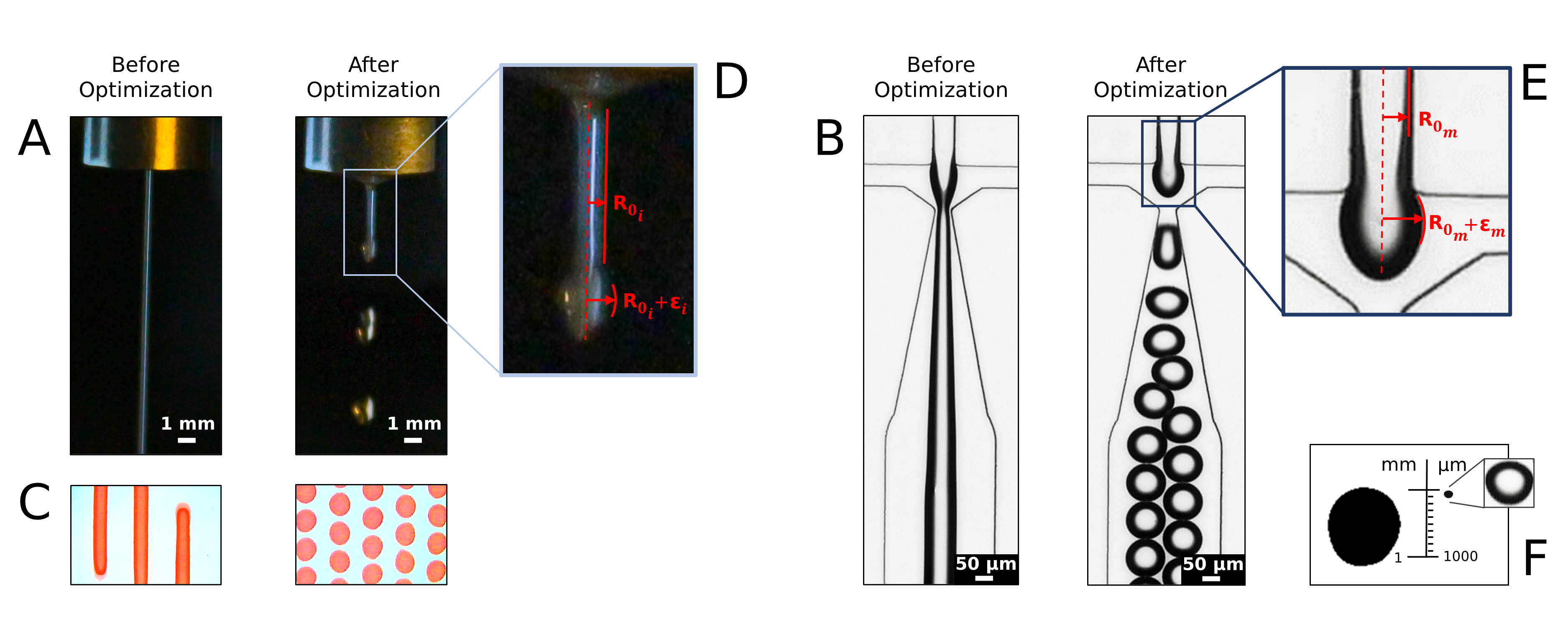
Figure 1: Fluid flow before and after control parameter optimization to form droplets. (A) Rayleigh instability and (B) capillary instability forming after optimization for the inkjet and microfluidics devices, respectively. (C) Deposited droplet patterns from the inkjet device. The images show a case from before optimization, using Latin hypercube sampled control parameter values, and a case from after optimization. Our model learns how to optimize droplet, which indirectly optimizes (D) Rayleigh and (E) capillary instabilities within the fluid stream. Rayleigh instability forms within the inkjet device by applying piezoelectric-driven perturbations, $\varepsilon_{i}$, to a water flow of radius $R_{0_{i}}$ being acted on by gravity in ambient air. Capillary instability forms within the microfluidic device by applying viscous stress-driven perturbations, $\varepsilon_{m}$, from the oil medium to a water flow of radius $R_{0_{m}}$. (F) Length scale comparison of an inkjet-generated droplet (left in mm) and a microfluidic-generated droplet (right in $\mu$m).

Generating discrete and uniform droplets from a fluid stream requires the fine-tuning of experimental conditions to transition the flow from a continuous, stable jet to a separated, unstable stream of droplets ¹. Rayleigh-Plateau instability governs the separation of a fluid stream into discrete droplets through gravity-driven perturbations and capillary instability governs the separation of a fluid stream into discrete droplets through pressure-driven perturbations ². Analytical relationships between governing parameters and droplet characteristics simply do not exist due to the complex, non-linear physical relationships between all forces acting on the fluid at various length scales ³. Thus, it is analytically intractable to determine the parameter values that produce optimized droplets, hence, requiring experimentation. Typically, researchers tune experimental controls until they reach the desired droplet characteristics ^{4, 1, 5, 6}. Our method provides an efficient way to find the appropriate values of experimental control parameters that achieve the desired outcome without developing a device-specific control model. Thus, we are no longer restricted to using our method only on devices with similar governing physics. We demonstrate that the method successfully optimizes droplets generated by devices that have both dissimilar control parameters and droplet length-scales, with few modifications. Furthermore, the novelty of our approach lies not only in its flexible application to devices with different governing physics and control parameters, but also in it requiring no upfront time to train, enabling researchers to quickly apply our method to their data and get results within hours rather than days ⁷.

Prior works develop proportional integral derivative (PID) controllers or classification machine learning to predict or control droplet states ^{8, 7}. However, both of these approaches are inflexible as they either require specific models to simulate the physics of a specific device, in the case of PID, or require training on large datasets of data specific to a single device, in the case of classification. Additionally, it has been shown that an estimated three days of upfront training is necessary to effectively classify and predict the droplet states of a microfluidic device ⁷. Our method requires no upfront training, instead, our algorithm learns the dynamics between input control parameters iteratively as the researcher performs experiments. We demonstrate that after initialization, our method requires only four rounds of experimentation with a batch size of 10 before converging on an optimum. Resulting in an average total optimization time of 2 hours, compared to previously reported $>70$ hours via supervised classification ⁷.

Flexible machine learning (ML) processes, such as Bayesian optimization (BO), have the promise to greatly improve the efficiency of exploring parameter spaces by saving expensive lab time and resources as they are generalizable to parameter spaces of varying dimensionality and require no upfront model training since they use a Gaussian Process (GP) backbone ^{9, 10, 8, 11, 12}. In this paper, we develop a universal BO and computer vision feedback loop to quickly and reliably discover Rayleigh and capillary unstable conditions in different droplet-generating devices with different governing control parameters and physics ^{13, 14}. We demonstrate the functionality of our method on two devices: (1) an milliscale inkjet droplet-generator with the controllable parameters of (a) pressure, (b) actuation frequency, and (c) translation speed and (2) a microfluidic droplet-generator with the controllable parameters of (a) water pressure and (b) oil pressure, shown in Fig. 1 and Fig. 3.

The challenge faced in optimizing droplets at different length scales is in designing a tool robust enough to predict the physics of each device parameter space to make meaningful and reliable predictions of optimized printing conditions. The challenge is addressed in this paper through our physical model-agnostic approach of optimization, which implements computer vision to detect the droplet flows and converts them into numerical representations of the parameter space for the Bayesian inference algorithm to learn. The significance of developing a tool that rapidly optimizes droplets at multiple length scales is in providing researchers with a universal tool for tuning devices that requires little customization or ML expertise. Generating these optimized droplets has importance across several application fields depending on the length scale of the droplet.

1.1 Prior Work on Millimeter-scale Droplets

Depositing millimeter-scale droplets onto a substrate is a process useful for high-throughput characterization of material, most notably for finding optimized semiconductor materials that maximize efficiency or stability ^{15, 16}. Semiconductors such as perovskites have vast and complex composition spaces which makes it challenging to discover optimum compositions ^{17, 18, 19}. Thus, using discrete inkjet-deposited droplets of varying semiconductor compositions for high-throughput experimental characterization elicits an accelerated search of this vast composition space for an optimum composition. However, studies such as Bash et al., (2020) rely on a domain expert to fine-tune experimental conditions that establish flow instability control prior to semiconductor characterization and, hence, require and understanding of system physics prior to optimization. Rather, in this study, the non-linear physical relationships between control parameters are iteratively learned by the probabilistic ML surrogate model as data is collected.

1.2 Prior Work on Micrometer-scale Droplets

Creating microspheres with a high surface area to volume ratio is beneficial for a large variety of applications such as materials generation, bio(chemical) analysis, polymeric microcapsules, and more ^{20, 21, 22}. Industries like food science, biomedical, and cosmetics use microcapsules as materials delivery vehicles with the ability to tune the capsule wall chemistry for slow or triggered release of the capsulated material ^{23, 24, 25}. For each of these unique applications, a different microdroplet volume is required. However, these droplet volumes and structures are a function of several physical parameters like the interfacial tension between the immiscible fluids, their viscosities, the microfluidic device geometry, and fluid flow rates ^{26, 27}.

Existing literature uses supervised neural networks to inform device geometry or to classify different control states for droplet generation. This method requires a large quantity of training data and requires an estimated 70 hours for model training. However, a gap still exists on how ML can be applied to optimize the device control parameters using GP techniques that do not require a priori training and can, in turn, operate much faster ^{28, 7}.. Thus, in this study, we use Bayesian inference methods to optimize the microspheres using the control parameters of water and oil pressures directly, rather than developing a PID model or supervised neural network to simulate the physical parameters and their non-linear relationships.

1.3 Main Findings

We demonstrate accurate and repeatable discovery of Rayleigh and capillary unstable regions to generate droplets of high yield and high circularity within two fluid devices at different length scales using Bayesian optimization and computer vision. For each of these fluid devices, three trials of Bayesian optimization were run using three different decision policy acquisition functions in which all trials converged to learning similar bounds for generating high circularity and high yield droplet structures. Convergence on optimized control parameters is attained for both devices using the same method within 2 hours while synthesizing 60 samples only.

2 Methods

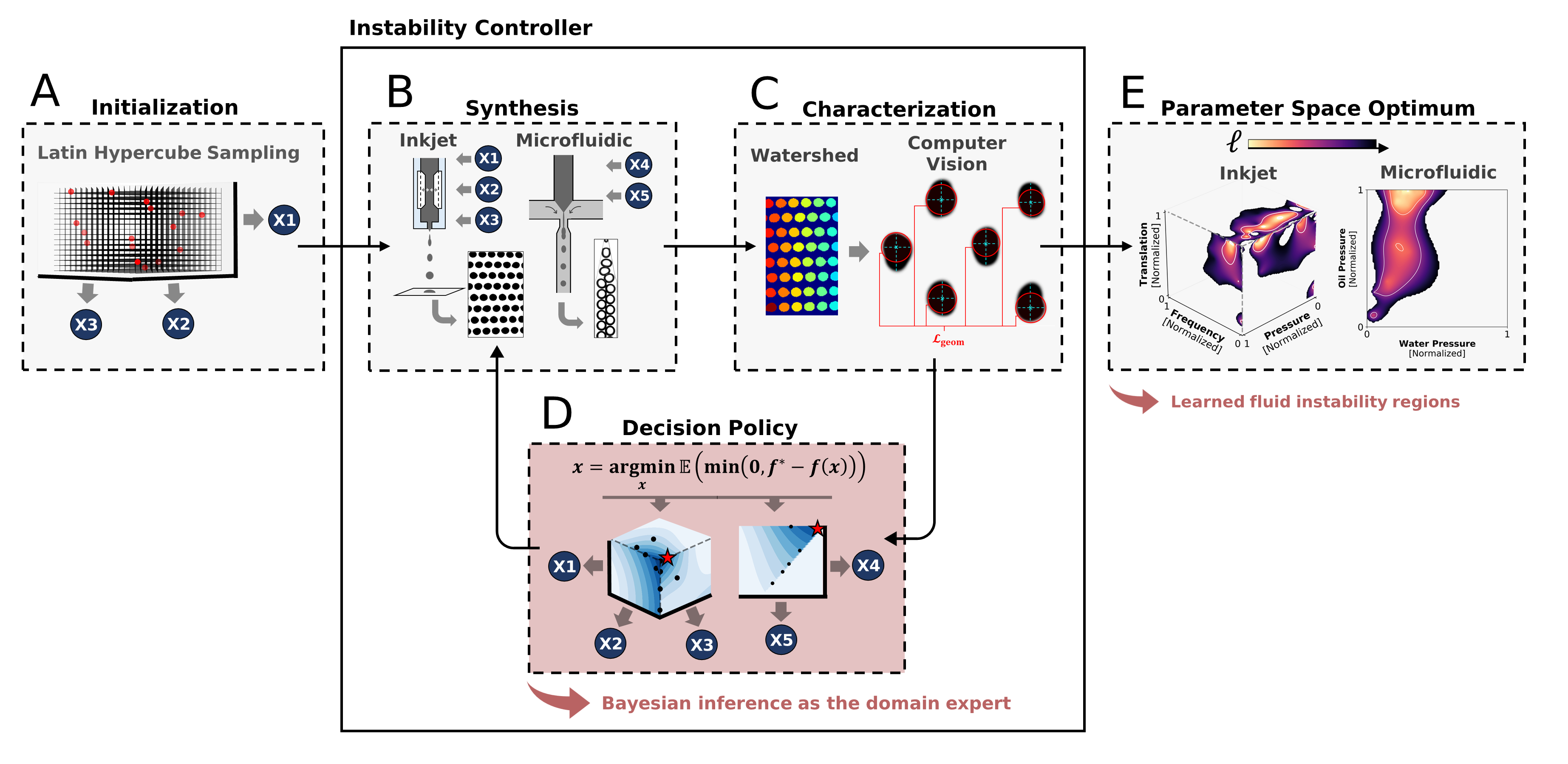
Figure 2: Control feedback loop of the hardware-algorithm interface used for droplet optimization. (A) The BO experiment is initialized using LHS, which samples control parameter values from the device parameter space. (B) For the first loop, LHS parameter values are used to print and image droplets. For proceeding rounds, learned parameter values by BO are used to print and image droplets. (C) Computer vision is used to score each droplet image and assign a label that quantifies droplet circularity and yield. The hardware (B) and computer vision (C) subsystems interface with each other by simply providing an image of the output droplets to the computer vision code. (D) The label and parameter values from the current loop and all prior loops are input into the BO decision policy directly from the computer vision algorithm, which informs the next round of parameter values to print. The iterative retraining of BO from processes (B)–(D) autonomously drives the control of the Rayleigh and capillary instability phenomena without a priori domain knowledge of a physical model. (E) Convergence on optimized control parameter values is assessed after four loops of iteratively retraining BO with new experimentally generated data.

Fig. 2 illustrates the workflow presented in this paper for multiscale droplet optimization. The user collects a set of initialization images of droplets generated from the device over a range of experimental control parameters (e.g., fluid pressures, nozzle frequency). The optimization software analyzes the data and generates a new set of control parameters to be used in the device, and the process is then repeated. Within only a few iterations, the efficient algorithm converges to a set of control parameters to produce the desired drops.

2.1 Device Hardware

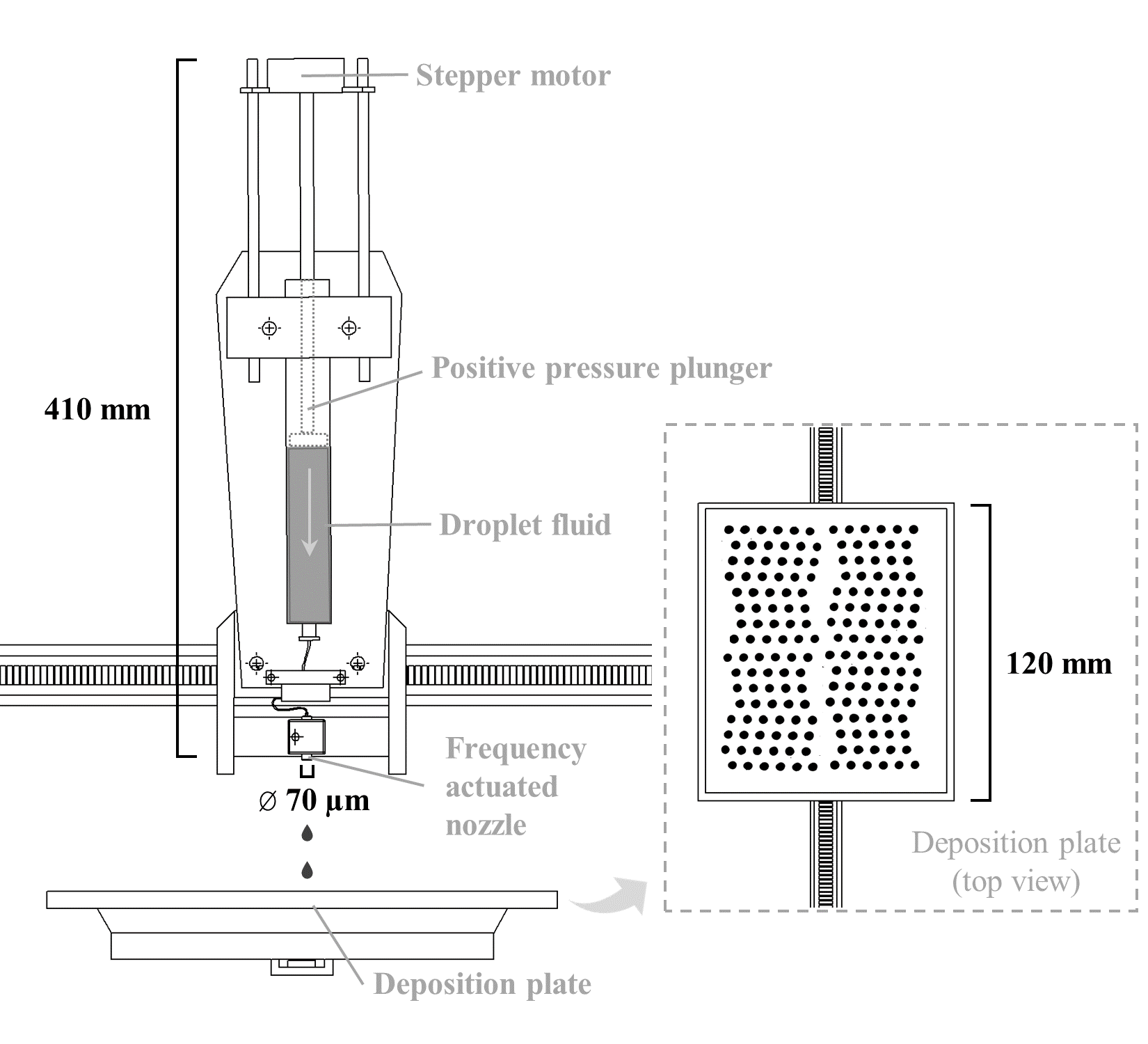
(a) Inkjet Device Architecture

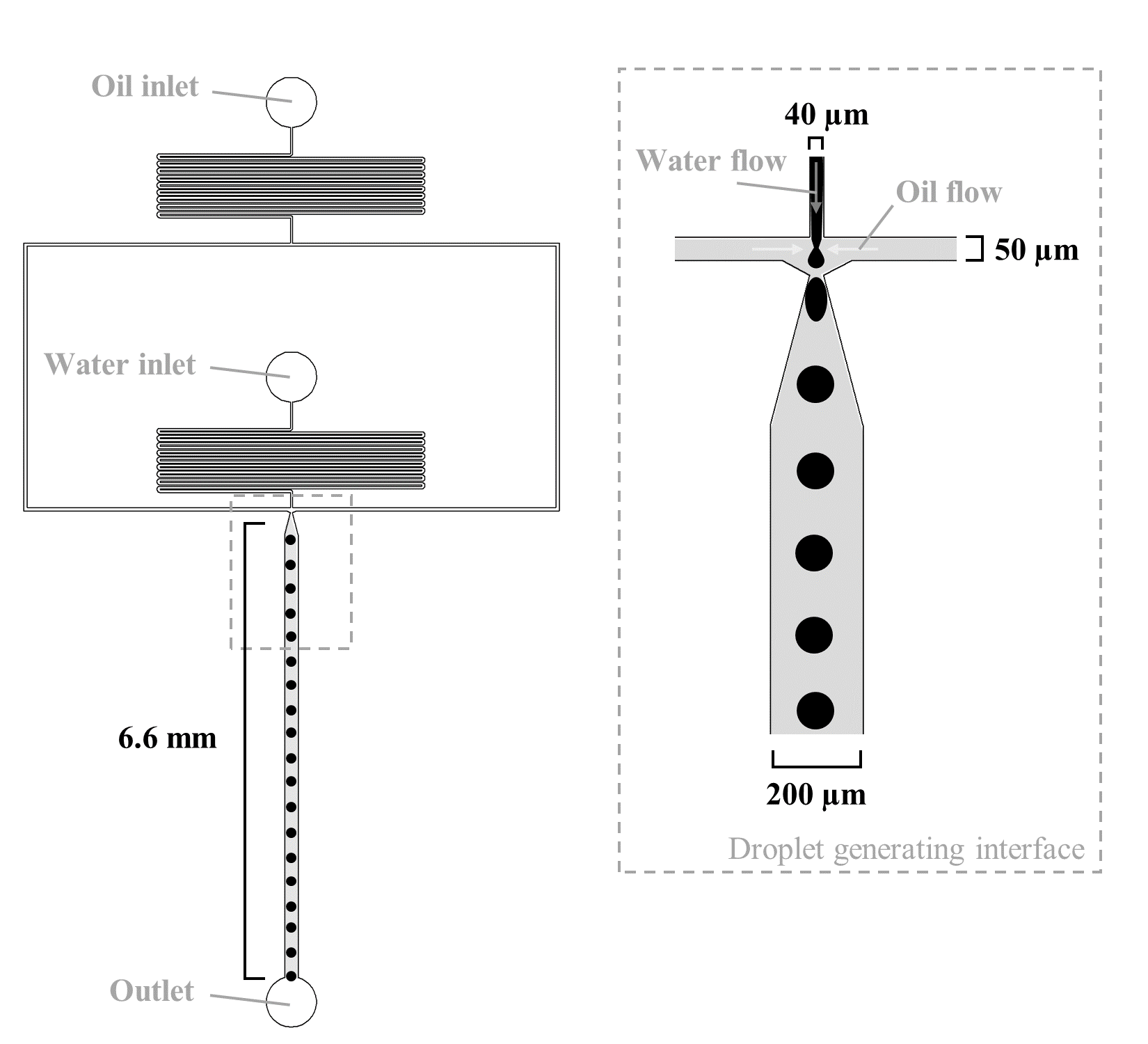
(b) Microfluidics Chip Architecture

Figure 3: Droplet-generating device hardware used in this study. (a) Inkjet device with inset image showing the top view of the deposition plate and the (b) microfluidics device with inset image showing the droplet generating interface. For the inkjet device, the positive pressure motor controls the fluid pressure in the vials; the frequency of the actuated nozzle controls the rate of droplet deposition; the speed of the laterally translating plate controls the droplet deposition placement. For the microfluidics device, the channel is flowed with mineral oil from the oil line as the suspending fluid; oil pinches off water from the water line to form droplets; all fluid exits through the outlet. The entire microfluidics device has a height of 30 $\mu$m.

2.1.1 Inkjet

The inkjet device has three possible control parameters: (1) fluid pressure, (2) piezoelectric actuation frequency, and (3) nozzle translation speed, of which we know the discrete values of at all times, but do not know the combination of these values that produce optimized droplets. These three parameters influence the shape and yield of droplets deposited on a plate ⁶. Pressurizing the fluid within the pipes drives both the radius and the flow rate of the stream for a fixed orifice size; our inkjet device operates at pressures limits of 0.03–0.15 MPa. Applying an alternating current electrical signal to the piezoelectric material within the pipe actuates a membrane at a given frequency to induce perturbations, $\varepsilon$, within the fluid stream ^{13, 14}; our inkjet device operates at frequency limits of 1.0–600.0 Hz using. The fluid is ejected from a nozzle which translates in 1D above a deposition site, which also translates in 1D perpendicular to the nozzle, driving 2D deposition of the fluid onto the deposition plate; our inkjet device operates at translation speed limits of 10–360 mm/s. None of these three control parameters are artificially constrained, the limits are defined by the physical limits of the hardware only. We keep both the fluid (dyed water) and nozzle diameter (70 $\mu$m) constant for all experiments, shown in Fig. 3(a). The intrinsic fluid properties are constant and we operate at flow velocities between 0.8–4 m/s, given the range of operating pressure. For every printed sample, these known values of the control parameters are appended to the image and normalized to a range of $[0,1]$ before being fed into the BO algorithm.

The printable fluid parameter space is governed by the fluid density, surface tension, viscosity, as well as the driving pressure and nozzle geometry ^{29, 30, 31}. While analytical relationships between these variables and the output droplet circularity and yield are intractable, the droplet properties can be described by dimensionless relationships between forces: (1) Ohnesorge number (Oh), which compares viscous forces to inertia and surface tension, (2) Weber number (We), which compares inertial forces to surface tension, and (3) Reynolds number (Re), which compares inertial to viscous forces ^{29, 30}.

$$\textrm{Oh}=\frac{\mu}{\sqrt{\rho\sigma d}},\qquad\textrm{We}=\frac{\rho v^{2}a}{\sigma},\qquad\textrm{Re}=\frac{\rho vd}{\mu},$$ (1)

where $\mu$ is the fluid dynamic viscosity, $\rho$ is the fluid density, $\sigma$ is the surface tension, $d$ is the jet diameter, $a$ is the droplet diameter, and $v$ is the characteristic flow velocity. Oh depends on fluid properties and nozzle diameter only, and so is fixed in our system at $\textrm{Oh}\approx 0.01$. This value falls in the range typically considered to facilitate satellite-drop formation; we observe satellite drops in approximately 10% of the inkjet samples ²⁹. Moreover, we determine the ranges of the variable dimensionless numbers to be $\textrm{We}\approx$ 1–200 and $\textrm{Re}\approx$ 10–50, which are further discussed in the results. Gravity is negligible in our system because the Bond number $=\frac{\rho gd^{2}}{\sigma}\approx 0.001$, where $g$ is gravitational acceleration, implying that capillary forces dominate the gravitational forces. Interestingly, despite operating in the regime of satellite drops, the data-driven BO approach efficiently explores and optimizes the parameter space for desired drop properties.

2.1.2 Microfluidic

The microfluidic device has two possible control parameters: (1) pressure to drive the inner droplet fluid (water) and (2) pressure to drive the outer suspending fluid (mineral oil), of which we know the discrete values of at all times, but do not know the combination of these values that produce optimized droplets. Both the water and oil pressure are controlled by a flow controller (Flow-EZ, Fluigent); our microfluidic device operates at pressure limits of 0-2000 mbar. Neither of these two control parameters are artificially constrained, the limits are defined by the physical limits of the hardware only. The outer mineral oil pinches off droplets of the inner DI water at a junction that is 40 $\mu$m wide, the droplets then travel into a channel 200 $\mu$m wide, shown in Fig. 3(b); the entire device has a height of 30 $\mu$m. Microfluidic droplet makers operate in one of five regimes at any given time: no inner fluid flow, unbroken inner fluid flow, dripping, transition, and jetting ^{32, 33, 34}. Our experiment explores two out of the three drop generation regimes: (1) dripping, where the drop forms while touching the constriction walls, and (2) transition, where the drop forms in the constriction without touching the walls. Jetting does not occur in our experiments due to the device structure, fluid viscosities, and experimental parameter space ³². Similar to the inkjet device, for every printed sample, the control parameters, normalized to the range $[0,1]$, are appended to the image and fed into the BO algorithm.

The droplet properties in the microfluidic system are primarily described by two dimensionless numbers: (1) Capillary number (Ca), which compares viscous forces to surface tension and (2) Weber number (We), which compares inertial forces to surface tension ^{35, 5, 36, 32}.

$$\textrm{Ca}=\frac{\mu\dot{\gamma}a}{\sigma},\qquad\textrm{We}=\frac{\rho v^{2}a}{\sigma},$$ (2)

where $\mu$ is the viscosity of the outer fluid or continuous phase, $\dot{\gamma}$ is the shear rate, $a$ is the droplet diameter, $\sigma$ is the surface tension between the two fluids, $\rho$ is the density of the continuous phase, and $v$ is the characteristic flow velocity. The ranges of these dimensionless numbers within our system are found to be $\textrm{Ca}\approx$ 0.005–0.05 and $\textrm{We}\approx$ 0.0005–0.003, which are further discussed in the results. Viscous stresses dominate the inertial effects in the microfluidics system because $\textrm{Re}\approx$ 0.04–0.4.

2.2 Parameter Space Initialization

Without a priori knowledge of the parameter space dynamics from a domain expert, we look towards using machine learning methods, in particular, Bayesian optimization (BO), to learn the topology of the parameter space. As more experimental data is acquired, BO refines its search of the parameter space for optimized printing conditions. The user collects training data over the range of parameter space in which optimization is desired. For the purpose of this demonstration, data was collected over the entire range of experimentally accessible parameters within our system.

To give BO the best chance at finding a global optimum condition, we provide the algorithm with our best estimation of the parameter space as a whole in the form of an initialization dataset. Latin hypercube sampling (LHS) is a sampling tool that generates an initialization sample set $\mathbf{x}\in\mathcal{X}^{(N)}$ to capture the variability of an $N$-dimensional parameter space with low bias ³⁷. LHS stratifies the range of each control parameter into $K$ strata ($K=20$ in this paper) of equal marginal probability such that each stratum is randomly sampled once to generate $\mathcal{X}^{(N)}$. The low variance demonstrated by LHS in literature, relative to random and stratified sampling, illustrates the goodness of LHS as an unbiased estimator for selecting initialization conditions ³⁷.

2.3 Computer Vision Characterization

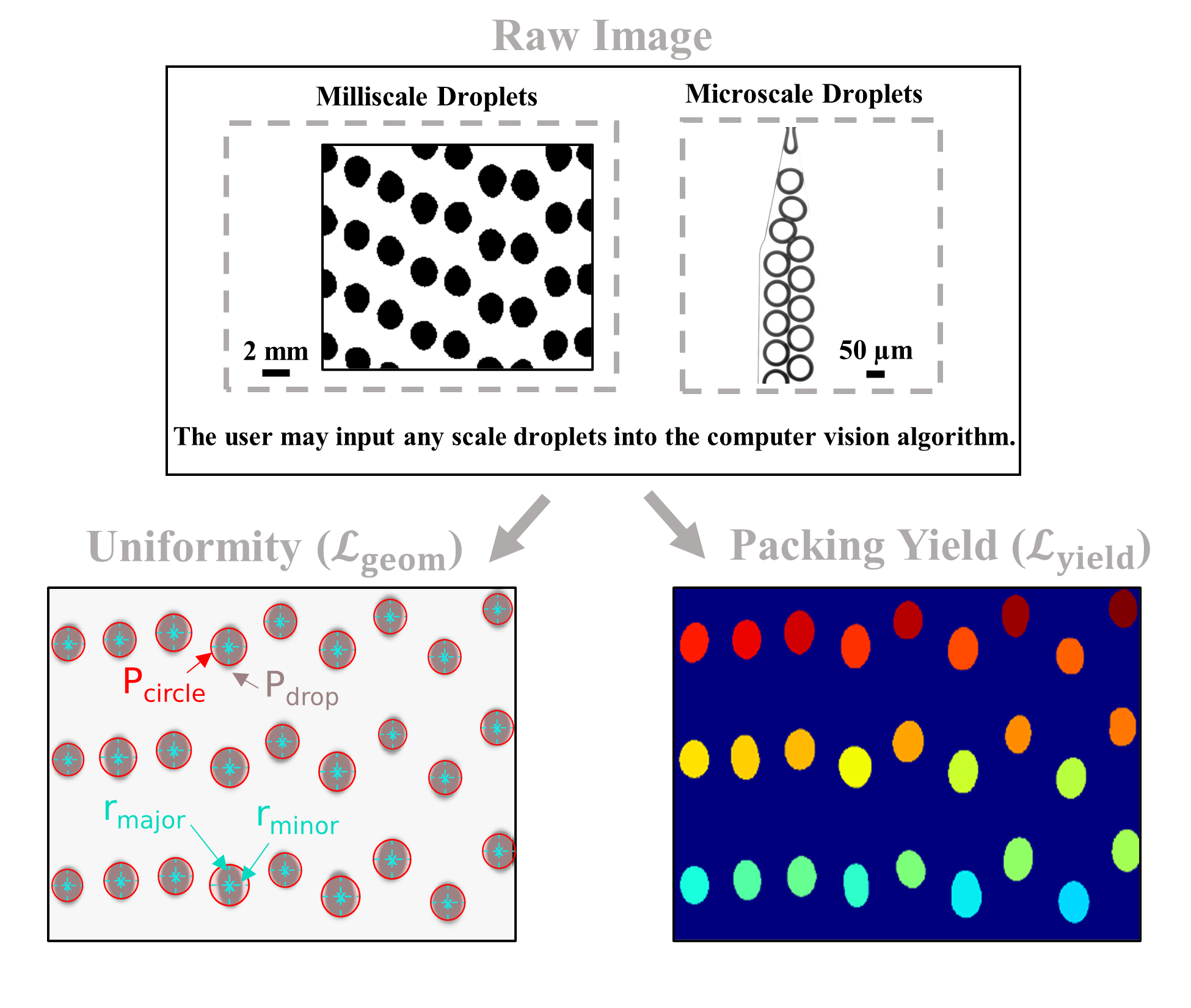
Figure 4: Computer vision characterization of droplets based on circularity and yield targets. The watershed process segments the droplets from the image background such that $\mathcal{L}_{\textrm{geom}}$ and $\mathcal{L}_{\textrm{yield}}$ can be computed. The developed computer vision code is robust to variations in droplet size, allowing for optimization of droplets at several scales, without adjustment – in this paper, milliscale and microscale droplets are explored. The developed computer vision algorithm is robust to variations in image artifacts by using pre-processing thresholds such that uniform image normalization is achieved.

The user can define a target. We defined our targets to be the geometric circularity and yield of droplets, as shown in Fig. 4. An optimization objective label $\ell$ is computed for each droplet sample via computer vision, which quantifies these properties of the droplet flow. A simple scalarized linear combination of loss functions is implemented to support flexibility of the user to implement their own loss functions.

After generating each sample, the flow is imaged and fed into the computer vision software. The computer vision software utilizes a watershed segmentation process flow ³⁸. The watershed process defines a dynamic threshold to segment each droplet in the sample from the background, as shown in Fig. 4, such that we generate a set of indexed droplet pixels $P_{\textrm{drop}}$. We characterize all indexed droplets within a sample by the optimization objective label, $\ell\in[0,1]$, which we aim to minimize.

Droplet circularity is the first component of $\ell$ and it is calculated by computing the loss between all droplets in the image $P_{\textrm{drop}}$ and perfect circles mapped onto the centroids of each droplet $P_{\textrm{circle}}$.

$$\mathcal{L}_{\textrm{geom}}=\frac{\sum\overline{P_{\textrm{drop}}\cap P_{\textrm{circle}}}}{\sum P_{\textrm{drop}}}.$$ (3)

By computing the major axis chord $r_{\textrm{major}}$ and minor axis chord $r_{\textrm{minor}}$ of each indexed droplet, a perfect circle is mapped to each droplet such that the circle’s centroid is the intersection point of $r_{\textrm{major}}$ and $r_{\textrm{minor}}$ and the radius is the average of these chords. Fig. 4 illustrates the process of mapping a circle to each watershed indexed droplet in the sample. We aim to minimize $\mathcal{L}_{\textrm{geom}}\in[0,1]$ to achieve droplets of high circularity.

Droplet yield is the second component of the optimization objective and it is computed by taking the loss of all droplet pixels and all non-droplet pixels to minimize the number of non-droplet pixels.

$$\mathcal{L}_{\textrm{yield}}=\frac{1}{2}\frac{\sum\overline{P_{\textrm{drop}}}}{\sum P_{\textrm{drop}}\cup\overline{P_{\textrm{drop}}}}+\frac{1}{2}\frac{\max(\textbf{count})-\textbf{{count}}(P_{\textrm{drop}})}{\max(\textbf{count})},$$ (4)

where $\max(\textbf{count})$ denotes the maximum count over all $P_{\textrm{drop}}$, which keeps $\ell$ as a minimization problem. We aim to minimize $\mathcal{L}_{\textrm{yield}}\in[0,1]$ to achieve droplets of high area and high count.

The total loss function $\ell(\mathbf{x})$ is constructed by taking the average of $\mathcal{L}_{\textrm{geom}}$ and $\mathcal{L}_{\textrm{yield}}$, as is common practice in computer vision studies ³⁹. We give equal importance to the geometric circularity and yield objectives during optimization which is suitable for our purposes. Every experimentally generated sample is labeled with a value of $\ell$ such that we aim to minimize $\ell\in[0,1]$ to achieve droplets of both high geometric circularity and high yield. The objective function in this study is user-defined, meaning that other important measurable droplet properties can be explicitly included by the user and tailored on the basis of the application.

2.4 Bayesian Optimization

Algorithm 1 Droplet Optimization by BO in Loop

  Inputs:  (1) LHS-initialized set $\mathbf{x}\in\mathcal{X}^{(N)}$, the $N$-dimensional control parameter space.      (2) Batch size, $b$.

  

  Outputs: (1) Vector of optimized control parameter values, $\mathbf{x}^{*}=\underset{\mathbf{x}\in\mathcal{X}}{\operatorname{arg\ min}}\;\ell(\mathbf{x})$.         (2) Running minimum loss across all samples, $\ell^{*}=\textbf{{min}}(\ell(\mathbf{x}))$.

  

  Let $\ell(\mathbf{x})=\frac{\mathcal{L}_{\textrm{geom}}(\mathbf{x})+\mathcal{L}_{\textrm{yield}}(\mathbf{x})}{2}$, the scoring function from computer vision.

  Let $\ell(\mathbf{x})\in\mathcal{S}\;\forall\;\mathbf{x}\in\mathcal{X}^{(N)}$, the set of losses of the training samples.

  while no convergence do

     Learn: Estimate parameter space with the GP surrogate, $\ell_{\textrm{pred}}(\mathbf{x})\sim\mathcal{GP}(\cdot)$.

     Predict: Using an acquisition function $a\in\{EI,MPI,LCB\}$, predict control parameter values, $\mathbf{x}_{i}$ for sample $i$, which minimize $\ell_{\textrm{pred}}(\mathbf{x}_{i})$.

     Synthesize: Synthesize $b$ samples using $\mathbf{x}_{i}$ parameters and image the sample.

     Update: Update $\ell_{\textrm{pred}}(\mathbf{x}_{i})$ with the computer vision image measurement $\ell(\mathbf{x}_{i})$. Concatenate $\mathbf{x}_{i}$ to $\mathcal{X}^{(N)}$ and $\ell(\mathbf{x}_{i})$ to $\mathcal{S}$.

  end while

  return $\mathbf{x}^{*}$, $\ell^{*}$.

We drive the efficient discovery of unstable fluid conditions using BO in loop, shown in Algorithm 1, where previous batches of generated samples inform the next batch of generated samples. The control parameter values $\mathbf{x}\in\mathcal{X}^{(N)}$ and labels $\ell\in\mathcal{S}$ of previous batches serve as a likelihood to a probabilistic surrogate model, in this case a Guassian Process (GP) ⁴⁰. The GP utilizes a decision policy, called an acquisition function, to acquire new control parameter values $\mathbf{x}$ that better optimize $\ell(\mathbf{x})$ or explore new regions of the parameter space that may contain more optimized values of $\ell$. We aim to minimize $\ell(\mathbf{x})$ to find the control parameter conditions that produce highly circular and high yield droplets ^{12, 41}:

$$\mathbf{x}^{*}=\underset{\mathbf{x}\in\mathcal{X}}{\operatorname{arg\ min}}\;\ell(\mathbf{x}),$$ (5)

where $\mathbf{x}$ is an $N$-dimensional vector of printing condition in the set $\mathcal{X}^{(N)}$.

GP is the surrogate model used to predict how the droplet flow $\ell(\mathbf{x})\in\mathcal{S}$ changes as the control parameter values $\mathbf{x}\in\mathcal{X}^{(N)}$ change:

$$\ell_{\textrm{pred}}(\textbf{x})\sim\mathcal{GP}(\mu(\mathbf{x}),\kappa(\mathbf{x},\mathbf{x}^{\prime})).$$ (6)

A Gaussian prior, $\mathcal{N}$, is assigned to the initial GP likelihood of the objective function $\ell(\mathbf{x})$ to estimate its posterior mean $\mu(\mathbf{x})$ and (co)variance $\kappa(\mathbf{x},\mathbf{x}^{\prime})$ ¹²:

$$\mu(\mathbf{x}) =\mathbb{E}[\ell(\mathbf{x})],$$ (7)

$$\kappa(\mathbf{x},\mathbf{x}^{\prime}) =\mathbb{E}[(\ell(\mathbf{x})-\mu(\mathbf{x}))(\ell(\mathbf{x}^{\prime})-\mu(\mathbf{x}^{\prime}))].$$ (8)

In this work, three common acquisition functions are used to guide the iterative selection of $\mathbf{x}$ ^{12, 41}: (1) expected improvement (EI), (2) maximum probability of improvement (MPI), and (3) lower confidence bound (LCB). We introduce these three distinct acquisition functions to illustrate the robustness of the computer vision-BO in loop method for discovering control parameter values that produce unstable fluid flow in both milliscale and microscale droplet-generating devices.

We begin an experiment by initializing the algorithm using LHS. Then, we iterate interleaving sampling and update steps. For every iteration of the BO in loop, 10 new $\mathbf{x}$ are acquired using the acquisition function’s decision policy. The decisions of the acquisition function are based on the GP parameter space estimation of $\ell$, computed from the labeled batch set $\mathcal{X}^{(N)}$, which contains all previous batch results. These new $\mathbf{x}$ are concatenated to $\mathcal{X}^{(N)}$ and $\ell$ are concatenated to $\mathcal{S}$ before acquiring the next batch of $\mathbf{x}$. The decision policies for each acquisition function used in this study are detailed next.

2.4.1 Expected Improvement Acquisition

Expected improvement (EI) is a decision policy that samples optima $\mathbf{x}$ from the GP by evaluating the function $\ell(\mathbf{x})$ and comparing the value to the current running minimum function evaluation $\ell^{*}=\textbf{{min}}(\ell(\mathbf{x}))$. Since our batch size is 10 samples per iteration, the EI acquisition function outputs 10 samples that have the highest improvement from previous $\ell^{*}$ ^{11, 41}:

$$a_{\textrm{EI}}(\mathbf{x})=\int^{\ell^{*}}_{-\infty}(\ell^{*}-\ell(\mathbf{x}))\mathcal{N}(\ell;\mu(\mathbf{x}),\kappa(\mathbf{x},\mathbf{x}^{\prime}))\textrm{d}\ell.$$ (9)

A local penalization evaluator is used which penalizes points closely sampled to each other within a batch, thus, the best point is selected first, then the second best (within some distance), and so on.

2.4.2 Maximum Probability of Improvement Acquisition

Maximum probability of improvement (MPI) is a decision policy that samples optima $\mathbf{x}$ similarly to EI, however, MPI does not scale the function values proportional to the magnitude of improvement. This means that MPI computes the location where $\ell^{*}=\textbf{{min}}(\ell(\mathbf{x}))$ but does consider how much the function value $\ell$ improves from the current running minimum $\ell^{*}$. Thus, the acquisition of MPI is the same as EI but without the $(\ell^{*}-\ell)$ term ^{11, 41}:

$$a_{\textrm{MPI}}(\mathbf{x})=\int^{\ell^{*}}_{-\infty}\mathcal{N}(\ell;\mu(\mathbf{x}),\kappa(\mathbf{x},\mathbf{x}^{\prime}))\textrm{d}\ell.$$ (10)

2.4.3 Lower Confidence Bound Acquisition

Lower confidence bound (LCB) is a decision policy that samples optima $\mathbf{x}$ through an explicit trade-off scheme between exploitation and exploration. A pure exploitation acquisition function outputs optima $\mathbf{x}$ exactly at evaluated GP function mean values $\mu(\mathbf{x})$ that minimize $\ell$, i.e., where the standard deviation $\sqrt{\kappa(\mathbf{x},\mathbf{x}^{\prime})}$ about the mean is zero. A pure exploration acquisition function outputs optima $\mathbf{x}$ within some large number of standard deviations about the mean. The LCB acquisition function balances exploiting the GP mean values with exploring the GP variance by varying a hyperparameter $\beta>0$ ⁴¹:

$$a_{\textrm{LCB}}(\mathbf{x};\beta)=\mu(\mathbf{x})-\beta\sqrt{\kappa(\mathbf{x},\mathbf{x}^{\prime})}.$$ (11)

2.5 Evaluating Parameter Convergence

To evaluate the performance of the presented BO and computer vision method, we visualize the topology of the objective $\ell$ within the parameter space of each trial for both devices. First, density estimations of each experimentally sampled parameter are shown to illustrate the regions of the parameter space most searched by the tool for each device and each acquisition function. Next, a subset of the imaged droplet flows are shown. Finally, the measured $\ell$ are plotted within the parameter space to demonstrate the learning of the method. Parameters with low $\ell$ generate the most circular and highest yield droplet flows for both devices at both milliscale and microscale. We compute the sample efficiency of the method by determining how many sampled points fall within the feasibility bounds. We identify that $\ell<0.75$ demarcates conditions that can feasibly generate droplets.

3 Results

3.1 Experimentally Sampled Conditions

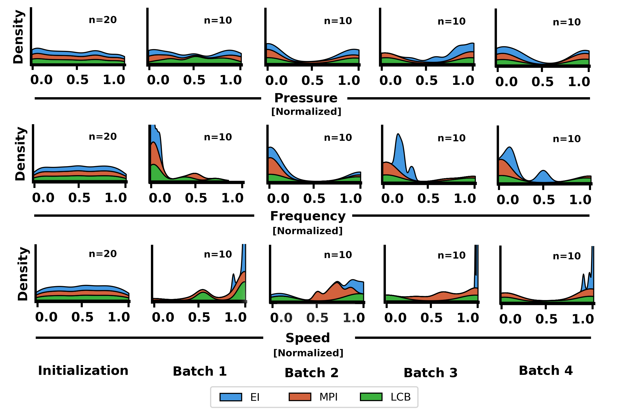
(a) Inkjet Control Parameter Sampling

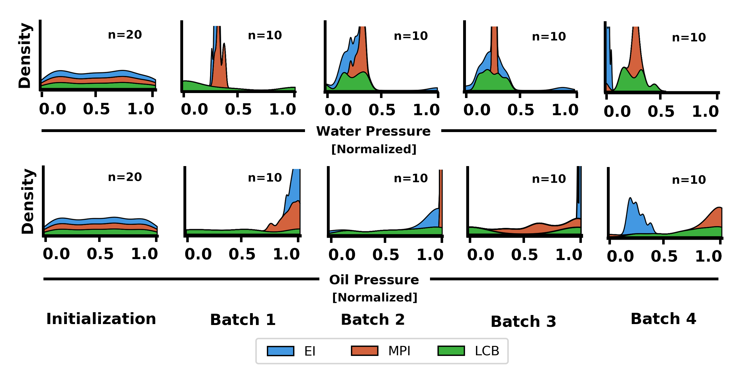
(b) Microfluidic Control Parameter Sampling

Figure 5: id=AES, comment=Adjust scale of this figure to improve readability.Density of control parameter values explored by each acquisition function over four batches of samples for the (a) inkjet device and (b) microfluidic device. As the number of batches increases, BO becomes more certain of what control parameter values produce the most optimized droplets.

The computer vision-driven BO in loop approach presented in this paper is demonstrated to consistently discover optimum control parameter conditions within both milliscale and microscale droplet-generating devices. Demonstrating the optimization capabilities of this approach at two different length scales illustrates its robustness and utility as a universal tool for experimentalists to tune their droplet devices without physics-based models, regardless of length scale. Furthermore, even though the phenomena of droplet breakup is governed by non-linear differential equations, our approach efficiently determines an appropriate set of experimental parameters to obtain the desired drops.

Fig. 5(a) illustrates the regions of the inkjet parameter space explored by each acquisition function for each batch of conditions acquired by BO in loop. It should be noted that these curves are density estimations of sampling frequency for each parameter and, thus, interpolate the shape of the curve between points. The inkjet device is driven by control parameters of pressure, frequency, and speed such that BO predicts parameters $\mathbf{x}\in X^{(3)}$ that minimize $\ell(\mathbf{x})$. For the pressure condition, it is shown that BO discovers samples across the whole range of pressures, indicating that the droplet flows are not sensitive to changes in pressure. Conversely, BO sampling is more concentrated for the frequency and speed conditions, indicating that high circularity and high yield droplet flows form using low frequency and high speed conditions.

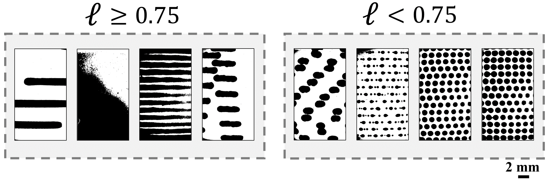
(a) Inkjet Droplets

(b) Microfluidic Droplets

Figure 6: Experimentally generated droplet samples labeled with the computer vision-computer optimization objective, $\ell$ for the (a) inkjet device and (b) microfluidic device. Control parameters that generate a sample with $\ell<0.75$ are shown to produce discrete droplets, hence, exhibiting the feasibility of Rayleigh and capillary instability occurring at those conditions. Conversely, control parameters that generate a sample with $\ell\geq 0.75$ are shown to have continuous or connected fluid flows, implying it is not feasible for Rayleigh or capillary instability to occur at these conditions.

Fig. 5(b) illustrates the regions of the microfluidic parameter space explored by each acquisition function. The microfluidic device is driven by two control parameters of water pressure and oil pressure such that BO predicts parameters $\mathbf{x}\in X^{(2)}$ that minimize $\ell(\mathbf{x})$. Unlike the inkjet device, the droplet flows are shown to be sensitive to both the control parameters in the microfluidics device. BO acquires points from low water pressure conditions and high oil pressure conditions.

The results from Fig. 5 illustrate the sampling mechanics of the GP-EI, GP-MPI, and GP-LCB BO models when all functions are initialized using the same dataset for each respective device. The regions of the parameter space where $\ell$ is minimized are learned using the sampling mechanics of BO. It will be shown that for each experiment, all of the tested BO models converge to similar optimum control parameters.

3.2 Learned Parameter Space Topology

Table 1: Time required to perform each process step in Bayesian optimization of droplets. Process steps are separated into whether it occurs on the software- or hardware-end of the optimization procedure. Averages and standard deviations of 12 model runs are shown, each run generating 10 droplet samples. The total time for convergence for 4 rounds of updates plus the initialization dataset is $total\ time\ per\ sample\ \textrm{[s]}*60$, since 60 samples are generated and analyzed for an entire optimization procedure.

Process Step	Time per Sample [s]	Type
Read Images	0.10 $\;\;\;\pm$ 0.01	Software
Computer Vision	2.7 $\;\;\;\;\;\pm$ 0.2	Software
Retrain Surrogate	0.40 $\;\;\;\pm$ 0.1	Software
Acquisition	0.50 $\;\;\;\pm$ 0.1	Software
Device Configuration	70.0 $\;\;\;\pm$ 10	Hardware
Print Droplets	30.0 $\;\;\;\pm$ 5	Hardware
Image Droplets	35.0 $\;\;\;\pm$ 10	Hardware
Total	3.7 $\;\;\;\;\;\pm$ 0.2	Software
Total	135.0 $\;\,\pm$ 15	Hardware
Total	138.7 $\,\pm$ 15	Both
	Time for Convergence [hr]
Total	0.062 $\;\,\pm$ 0.0004	Software
Total	2.25 $\;\;\;\,\pm$ 0.03	Hardware
Total	2.31 $\;\,\,\,\pm$ 0.03	Both

Our method discovers the control parameter conditions that produce droplets due to fluid instabilities at both the millimeter and micrometer scales using the same computer vision-driven BO in loop method. Table 1 notes the time required to perform each process step. Our method takes $138.7$ seconds per sample to run, and $2.3$ hours to run the full optimization procedure, compared to $>70$ hours via prior methods ⁷. The time for convergence is shown to be dominated by hardware calibration and synthesis processes (97.3% of total convergence time), rather than software processing or model training (2.7% of total convergence time). This is true since the learning process occurs in the loop and only $O(10^{1})$ data points are used in our GP approach, compared to the $O(10^{6})$ data points used for upfront training in prior neural network approaches ⁷. Fig. 6 illustrates a subset of droplet flows from stable flows, i.e., outside of the feasibility bounds, $\ell\geq 0.75$, and from unstable flows, i.e., inside the feasibility bounds $\ell<0.75$. Fig. 7 shows the parameter space topology of the objective values $\ell$ obtained from each experiment. It should be noted that topologies are Gaussian interpolated from the raw data for clarity; no extrapolation is done. The sample efficiency of each BO model is determined based on the number of sampled points that fall within the feasibility bounds – meaning that a model with higher sample efficiency requires fewer samples to achieve an optimum solution.

(a) Learned Rayleigh Unstable Conditions

(b) Learned Capillary Unstable Conditions

Figure 7: id=AES, comment=Increased figure font size.Control parameter values learned by BO to form (a) Rayleigh and (b) capillary instability to generate optimized droplets within the inkjet device and microfluidics device, respectively. Three rows of figures are illustrated, one row for each independent experiment run with a different acquisition function (EI, MPI, and LCB). The first column illustrates the values of all control parameter values sampled by all batches of BO over the course of the experiment. The second column illustrates the where BO has discovered that Rayleigh/capillary instability can occur within the parameter space ($\ell<0.75$). The third column shows the measured value of $\ell$ within the feasibility bounds. Lower values of $\ell$ denote more optimized droplet flows.

(a) Inkjet Drop Diameter

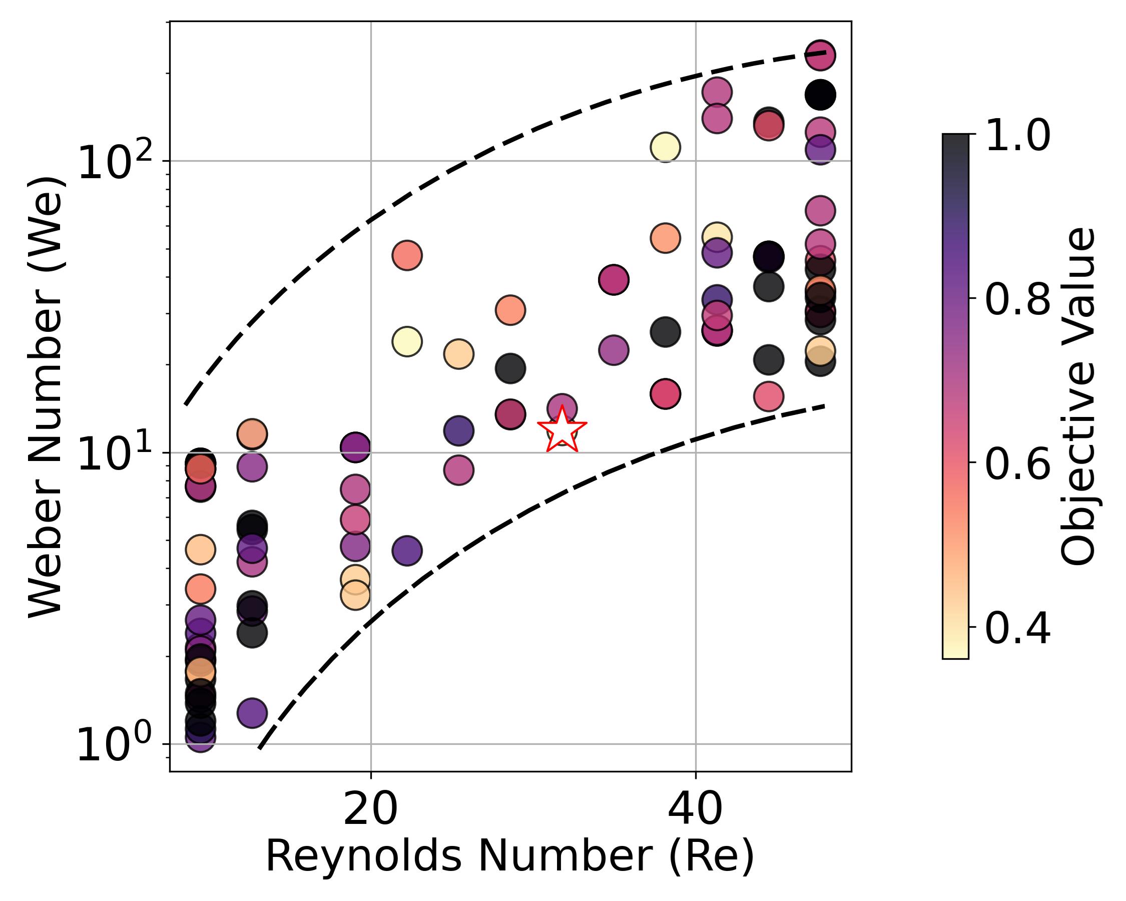
(b) Inkjet Objective Value

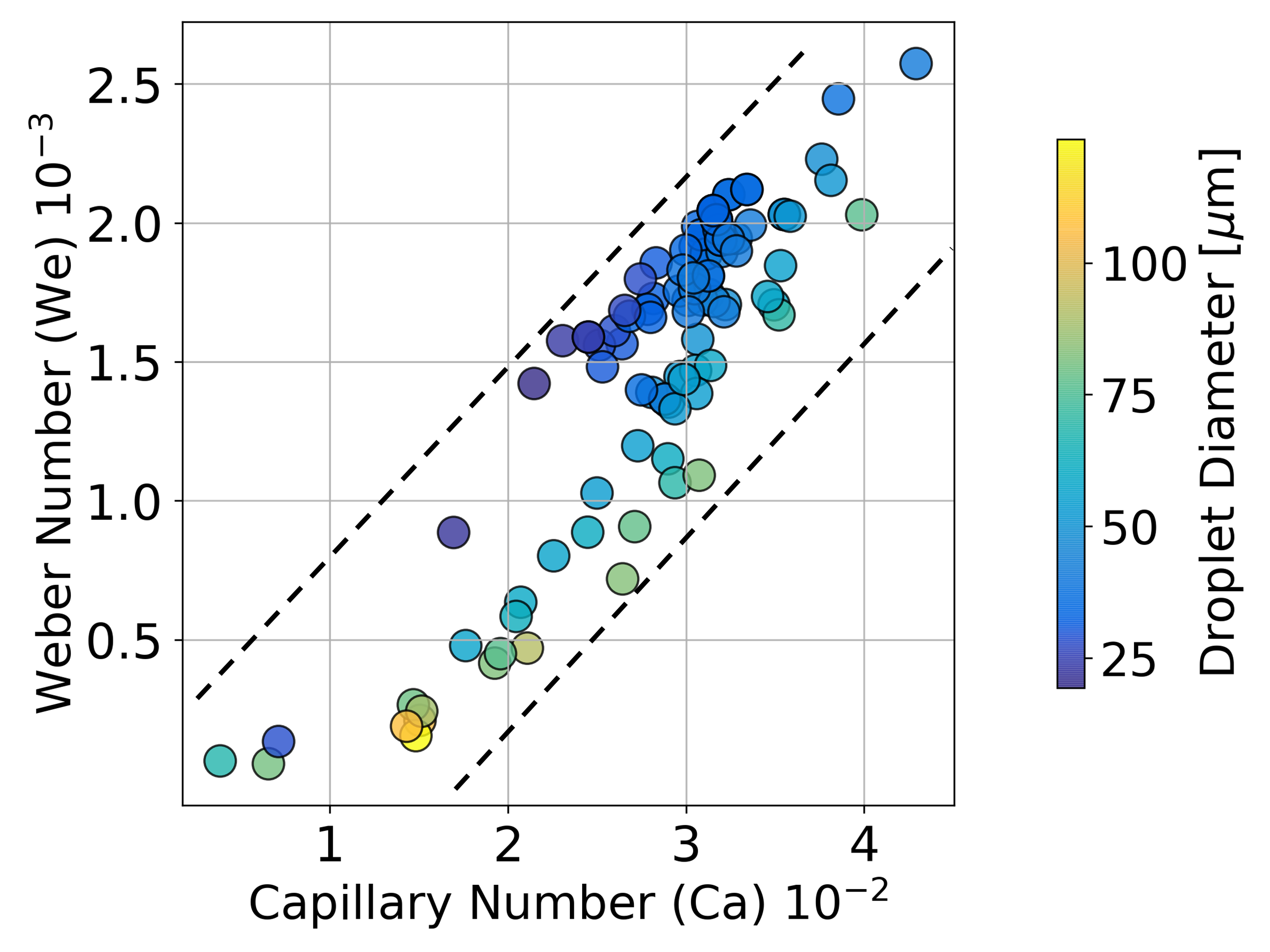
(c) Microfluidic Drop Diameter

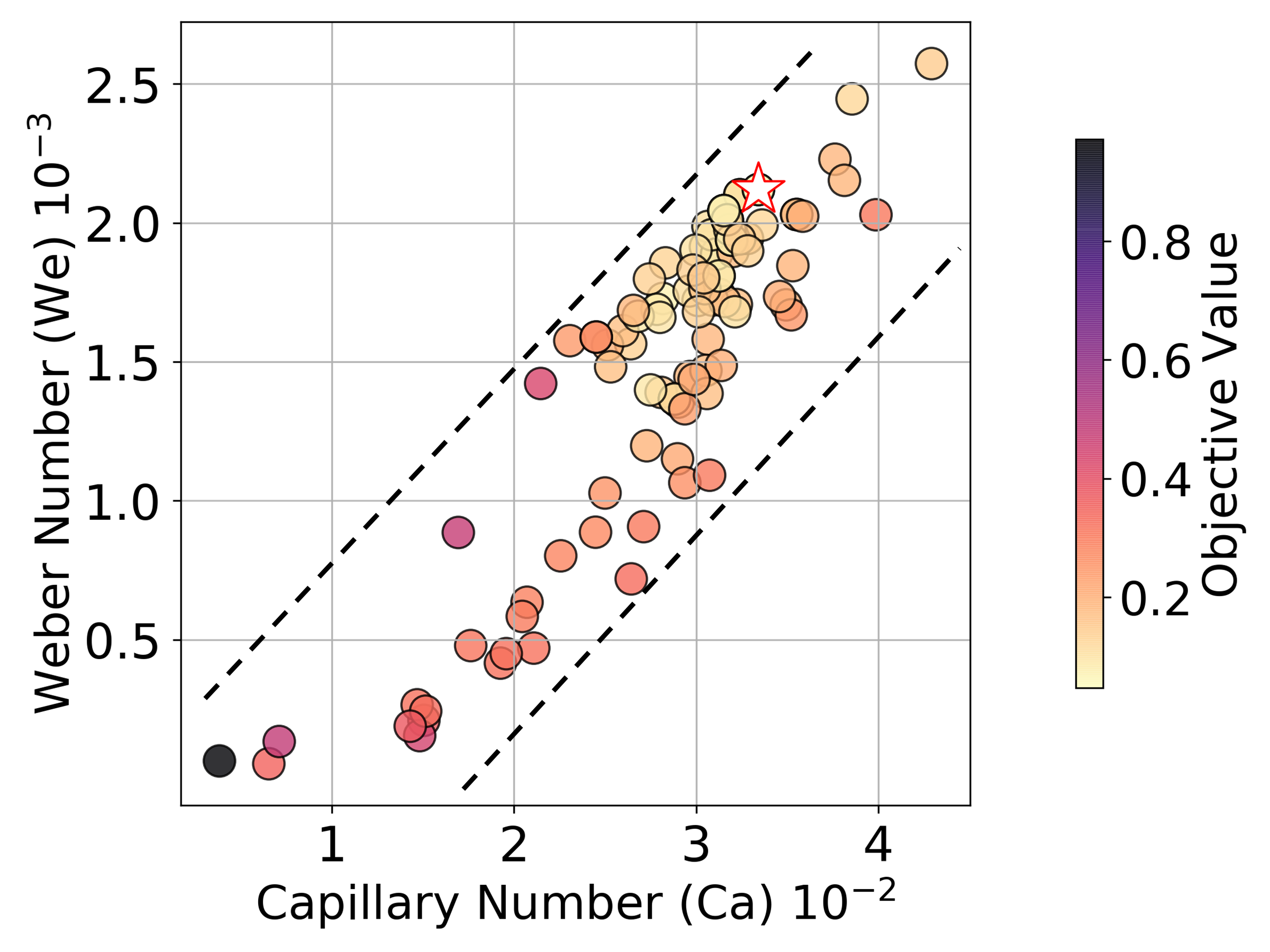
(d) Microfluidic Objective Value

Figure 8: Reynolds number versus Weber number for (a) inkjet drop diameter, (b) inkjet objective value, $\ell$; and capillary number versus Weber number for (c) microfluidic drop diameter, (d) microfluidic objective value, $\ell$. Each subfigure includes all $n=120$ synthesized droplet patterns across the three acquisition policy experiments, not including the initialization set. The dashed curves represent the envelop of the parameter space explored. For the inkjet device, the diameter of the in-air droplets are computed using a spherical end-cap and the measured contact angle ⁴². For the microfluidics device, the velocity and fluid density are referring to the continues phase (mineral oil) and the interfacial tensions for water in oil. The location of the most optimal droplet pattern, i.e., lowest objective value, is indicated as a white star in (b) and (d).

For the inkjet device, BO discovers the feasible control parameter values for Rayleigh instability to be in low-mid range frequencies and mid-high range translation speeds using different decision policy acquisition functions. Moreover, Fig. 7(a) illustrates that this instability may exist for all pressure values within the inkjet device. The importance ranking of each parameter-objective relationship is indicated using SHAP in Fig. 5(a) for the inkjet device ⁴³. The model sample efficiencies when integrated into the optimization of the inkjet device are: (1) 65.0% using GP-EI, (2) 45.0% using GP-MPI, and (3) 40.0% using GP-LCB. Fig. 8(b) shows a scatter plot of Re versus We for every inkjet-printed sample output by the BO model; the colorbar indicates the objective value. These experimental results illustrate the highly non-linear relationship between Re, We, and the objective value. Despite the complexity of this parameter space, our method is still shown to discover the correct optimized region of the parameter space as three independent experimental trials converge to the same optimum conditions, as shown in Fig. 7. These optimized conditions fall within the regions of the Re–We space that have optimal drop-on-demand printing conditions, as suggested in the literature ^{29, 44}. Our results in Fig. 8(b) validate the expectation that droplets do not reliably form due to Rayeligh instability at $\textrm{We}\lesssim 3$ ⁴⁴. The computed We may differ slightly from the expected value since the jet diameter contracts and expands as a function of velocity ⁴⁵. Comparing these results to Fig. 7(a) and Fig. S-2, the optimized parameter space is shown to correspond to low actuation frequency and fast translation speed throughout the pressure range. Additional information regarding the impact of control parameters on droplet optimization can be found in the Supplementary Information.

For the microfluidic device, BO discovers the feasible control parameter values for capillary instability to be in low-mid range water pressure values for the whole range of oil pressure values using different decision policy acquisition functions, as shown in Fig. 7(b). The importance ranking of each parameter-objective relationship is indicated using SHAP in Fig. 5(b) for the microfluidic device ⁴³. The model sample efficiencies when integrated into the optimization of the microfluidic device are: (1) 67.5% using GP-EI, (2) 97.5% using GP-MPI, and (3) 75.0% using GP-LCB. Predictions of droplet shape and size as a function of the device control parameters remain intractable to predict ¹⁴. Fig. 8(c)–8(d) illustrate the non-linear relationship between We, Ca, and the objective value, further demonstrating the significance of exploring the experimental configuration space via BO. The optimized objective value is found in the region $\textrm{Ca}\sim$ 0.03 and $\textrm{We}\sim$ 0.002. Comparing these results to the optimization shown in Fig. 7(b) and Fig. S-3, a roughly linear band, in which the oil and water pressures increase proportionally to each other, can be seen. However, the non-linear bounds on the learned optimized region in the parameter space, shown again in Fig. 7(b), are a reminder of the non-linear physics governing droplet formation and characteristics.

4 Discussion

Our work addresses the challenge of developing a universal tool for optimizing droplet-generating devices at multiple length scales. It is often the case where no analytical function exists to map device control parameters to a target material property, thus, resulting in wasteful trial-and-error experimentation to discover those optimized conditions. We demonstrate the ability of a computer vision-integrated Bayesian optimization framework to accurately and rapidly discover control parameter values with repeatability that optimize the generated droplets with no a prioi domain knowledge of the device. The significance of this paper is in providing a scale-invariant and physical model-agnostic method for droplet-generating devices optimization that can be used to flexibly optimize many different droplet-generating systems in $2.3$ hours.

We demonstrate that for these milliscale and microscale droplet-generating devices, a machine learning algorithm can learn which control parmeter values produce Rayleigh/capillary instabilities and, in turn, transition a continuous fluid stream to a decomposed flow of droplets. The performance of this method is demonstrated using three independent experiments for each device, each with a different acquisition function but with the same initialization dataset and surrogate model: (1) GP-EI, (2) GP-MPI, and (3) GP-LCB. After four batches of data sampling and model updates, all three experiments converge to similar optimized regions of the parameter space for both length scale devices. We illustrate the significance of our method in an application space where droplets optimized for high circularity and high yield do not always correspond with droplets of a certain size, see Fig. 8(a)–8(b), hence, demonstrating the power of a flexible ML method to predict the values of control parameters that optimize droplets. Convergence occurs within four rounds of sampling, resulting in a total average optimization time of $2.3$ hours, compared to $>70$ hours previously reported using supervised learning, hence, accelerating throughput by $30\times$ ⁷. Unlike previous literature where the majority of the optimization time is dominated by model training, the majority of optimization time using our method is dominated by running experiments on the device hardware. Therefore, this method provides an extremely fast way to optimize droplets within complex parameter spaces and has the potential to be accelerated further by an increase in experimental throughput.

For the inkjet device, converged conditions are the full pressure range, low piezoelectric frequencies, and high axial translation speeds. For the microfluidic device, converged conditions are low-mid water pressures and high oil pressures. However, each of these acquisition functions has a different sampling efficiency, indicating that the acquisition function affects the rate of learning differently depending on the length scale of the droplets generated by a device. The highest efficiency acquisition function for the inkjet device is GP-EI where 65.0% of sampled points are within the feasiblity bounds, whereas the highest efficiency acquisition function for the microfluidic device is GP-MPI where 97.5% of sampled points are within the feasibility bounds. The differences in these results can be explained by each device having different governing physics and a different number of control parameters that comprise the parameter space. Although GP-LCB results in a low sampling efficiency, it provides a powerful mode of exploration rather than exploitation, which could be used to improve our understanding of the governing physics of droplet formation across length scales. It should be noted that even though the acquisition function was varied in the computer vision-Bayesian optimization algorithm, all experiments results in convergence to optimized droplet flows.

5 Conclusion

We present a machine learning-based method for rapid optimization of several droplet-generating devices at different length scales. Tuning an experimental device to produce an optimized product is dynamic; the optimized conditions change based on the operating length scale of a device due to the governing physics of the device changing. Thus, there is the challenge to design a universal method for scale-invariant droplet optimization. In this study, we develop a method of Bayesian optimization in loop with computer vision characterization to discover the optimum conditions for generating droplets at two different length scale experimental devices in $2$ hours, without upfront model training.

Through several trials of experimentation, we demonstrate that our machine learning and computer vision approach discovers optimized droplet-generating device control parameter values at both the milliscale and microscale. Furthermore, our method does not require knowledge of droplet size dependence on control parameters, thus, this optimization approach is demonstrated to be scale-invariant. As no physical or mathematical model is required to perform optimization, this optimization approach is also demonstrated to be physical model-agnostic; meaning that this approach can be extended to explore more complicated devices like those using non-Newtonian fluids, polymeric fluids that crosslink in flow, or phase-change materials with few adjustments. Moreover, our method implements probabilistic surrogate model training and retraining in parallel with data acquisition, significantly reducing the time required to run the optimization procedure compared to methods of upfront model training. Developing this multiscale droplet optimization method provides researchers with a universal tool for accelerating smart device conditioning and reduces wasteful trial-and-error experimentation.

We thank James Serdy (MIT) for knowledge contributions and engineering expertise in hardware development and running physical experiments. We thank Dr. Armi Tiihonen for guidance and assistance with Bayesian optimization of physical systems. We thank Dr. Shijing Sun for contributions to methodology development and framing of this paper. This material is based upon work primarily supported by the Center to Center (C2C) International Collaboration on Advanced Photovoltaics as part of the Engineering Research Center Program of the National Science Foundation and the Office of Energy Efficiency and Renewable Energy of the Department of Energy under NSF Cooperative Agreement No. EEC-1041895. Iddo Drori would like to thank Google for a cloud research grant.

Data Availability. All data and code are available at https://github.com/PV-Lab/ML-Multiscale-Droplets

Conflict of Interest Statement. Author T.B. holds equity in a start-up company (Xinterra) focused on commercializing machine learning technologies for accelerated materials development.

Supporting Information. Additional information provided for the parameter space search of each decision policy, importance ranking of control parameters, relevant dimensionless numbers, and images of the experimental setups, including the data collected for all experiments.

GitHub: https://github.com/PV-Lab/ML-Multiscale-Droplets

6 For Table of Contents only

S-1 Supporting Information:
A Machine Learning and Computer Vision Approach to Rapidly Optimize Multiscale Droplet Generation

Alexander E. Siemenn,^∗,† Evyatar Shaulsky,^‡ Matthew Beveridge,^¶ Tonio Buonassisi,^† Sara M. Hashmi,^∗,‡ and Iddo Drori^∗,¶

${\dagger}$Department of Mechanical Engineering, Massachusetts Institute of Technology, Cambridge, MA 02139, USA

${\ddagger}$Department of Chemical Engineering, Northeastern University, Boston, MA 02115, USA

${\mathparagraph}$Department of Electrical Engineering and Computer Science, Massachusetts Institute of Technology, Cambridge, MA 02139, USA

E-mail: asiemenn@mit.edu; s.hashmi@northeastern.edu; idrori@mit.edu

For each loop of optimization, the regions of the parameter space where new optima are acquired by each decision policy are highlighted in dark blue in Figure S-2 for the inkjet device and in Figure S-3 for the microfluidic device. For each of these sampled batches, all of the acquired points are plotted as box plots to illustrate the ranges of objective values. This information is useful when designing a fluid device such that a researcher may engineer the device to have experimental parameter values within the regions of high acquisition value.

Figure S-4 illustrates the running minimum objective value across all sampled points for the inkjet and microfluidic devices. As the autonomous optimization procedure runs, more highly-optimized droplet structures are discovered.

The importance impact of each experimental parameter on the objective value $\ell$ is illustrated in Figure S-5. For the inkjet device, frequency is illustrated to have a much larger impact on the objective value compared to pressure and translation speed. For the microfluidic device, water pressure is illustrated to have only a marginally larger impact on the objective valued compared to the water pressure. These results are useful for designing new fluid devices since understanding the impact of a device’s input on the output product provides insight into which input parameters should receive more attention during tuning.

The parameter space envelope for each BO acquisition function shown in Figures 7 and 8. For a microfluidics device, the slope of the linear ratio correlation will change depending on the properties of the device ^{32, 5}. The width of the instability drop formation region will change as a result of the fluids characteristics such as viscosity ratio. In the high-valued regions of Ca and We numbers, the oil pressure exceeds the viscosity ratio and, in turn, results in no water flow or water backflow. Moreover, in the low-valued regions of Ca and We numbers, the water pressure exceeds the viscosity ratio and forms a continuous water stream instead of droplets. In the specific case of flow-focusing microsystem, the drop formation region can be divided into three distinguished sections. The first regime, "squeezing" or "geometric restriction", appears at the low flows/pressures and low capillary number area. The inner fluid is touching the restriction wall before breaking into individual drops ³⁶. In the squeezing regime, there is a good correlation between the drop size and the fluid flow fraction. The second regime, "dripping" or "transition" appearing at the mid-range flows/pressures and capillary number. In this regime, the formation of the droplets is due to an increased flow velocity inside the restrictions that leads to pinched off droplets. In this case, smaller droplets can be formed, and as we are increasing the fraction ratio between the inner and continuous liquids, a high volume of small drops is generated. The third regime is the "jetting" that appears at the highest pressures and capillary numbers, where the droplets form after the restriction.

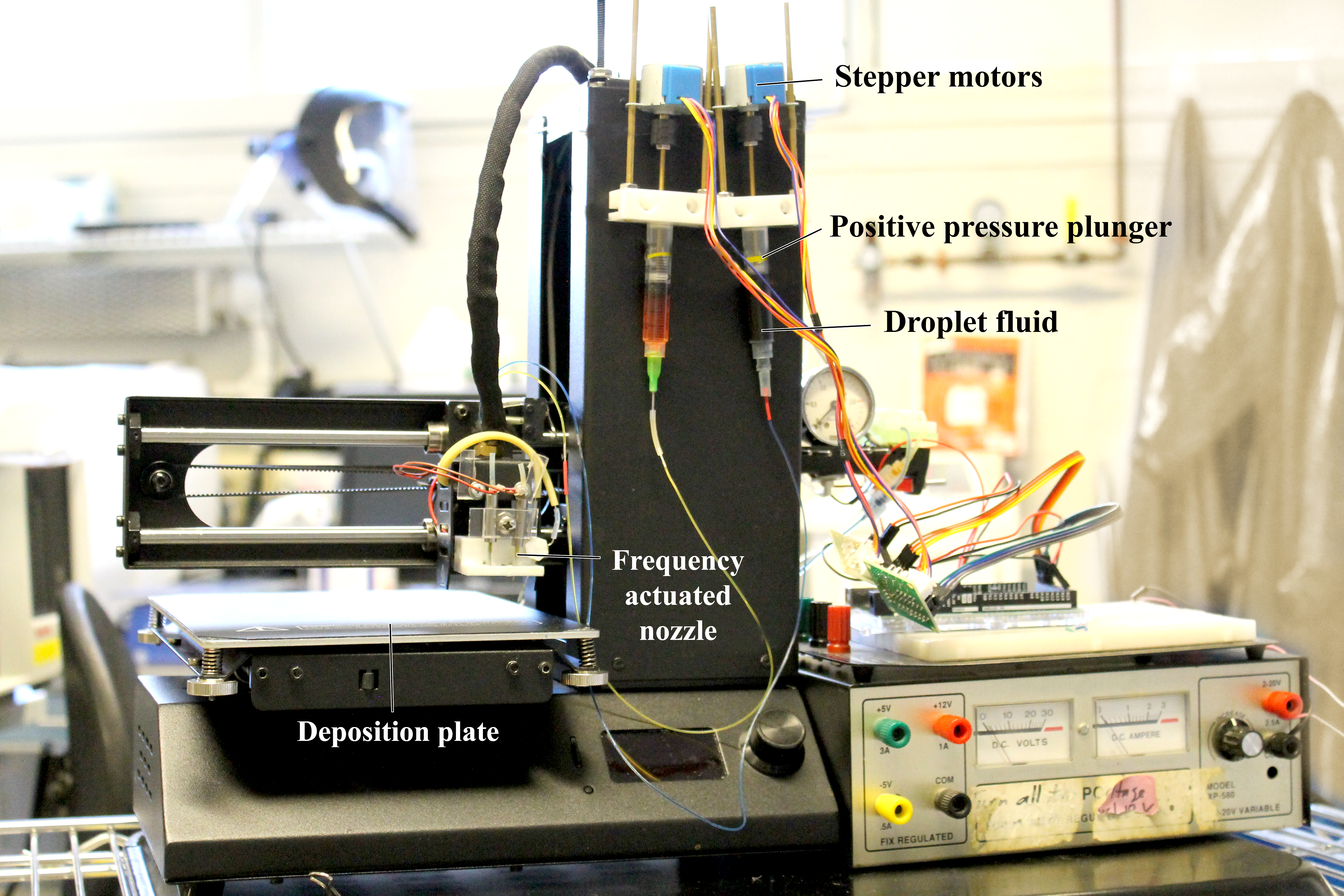
(a) Inkjet Device Hardware

(b) Microfluidics Device Hardware

Figure S-1: Images of the (a) inkjet droplet-generator and the (b) microfluidics droplet-generator.

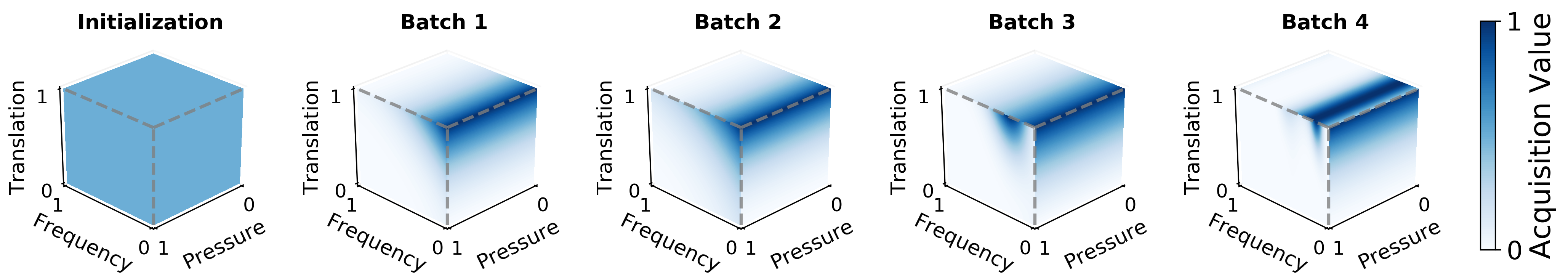
(a) Inkjet EI Acquisition Value per Batch

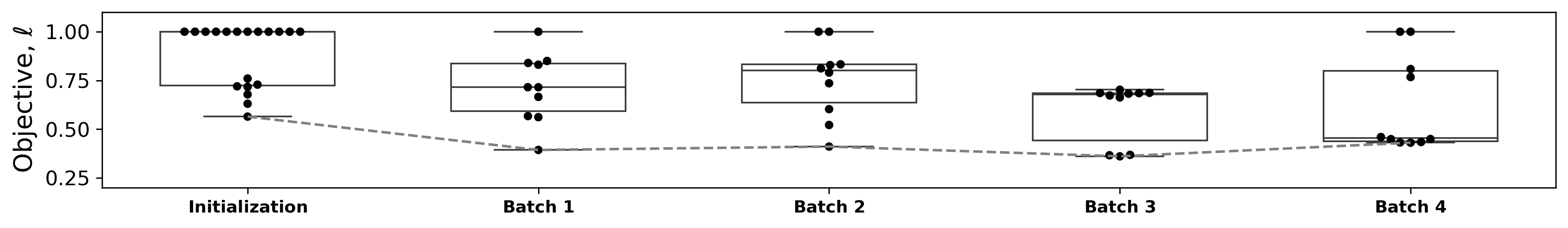
(b) Inkjet EI Objective Value per Batch

(c) Inkjet MPI Acquisition Value per Batch

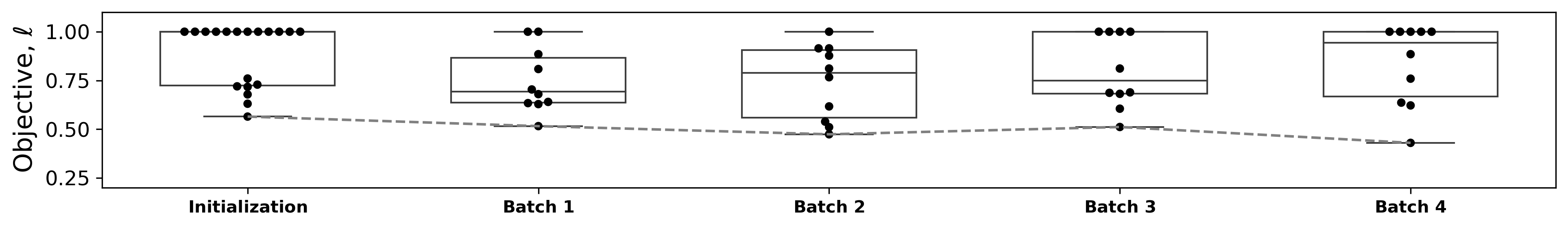
(d) Inkjet MPI Objective Value per Batch

(e) Inkjet LCB Acquisition Value per Batch

(f) Inkjet LCB Objective Value per Batch

Figure S-2: Acquisition function search spaces by batch in 3-dimensions. The regions where each acquisition function is likely to draw points from within the inkjet parameter space are illustrated in blue for each acquisition function: (a) EI, (c) MPI, (e) LCB – these denote regions of high acquisition value. The initialization acquisition space is a uniform color because points are picked uniformly during initialization via LHS. Based on the mechanics of each acquisition function, the acquisition value is computed by balancing the exploitation of the GP posterior mean and exploring the GP (co)variance. The acquisition search space evolves every loop, which updates the sampling locations of data points, shown for each acquisition function: (b) EI, (d) MPI, (f) LCB. The reason why the same data point that maximizes the acquisition value is not sampled 10 times for every batch in the loop is because of evaluator used is local penalization – points sampled close to each other are penalized, thus, the best point is selected first, then the second best (within some distance), and so on.

(a) Microfluidic EI Acquisition Value per Batch

(b) Microfluidic EI Objective Value per Batch

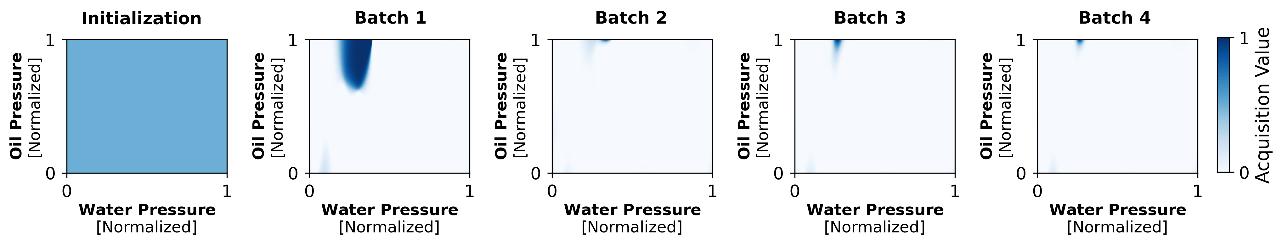
(c) Microfluidic MPI Acquisition Value per Batch

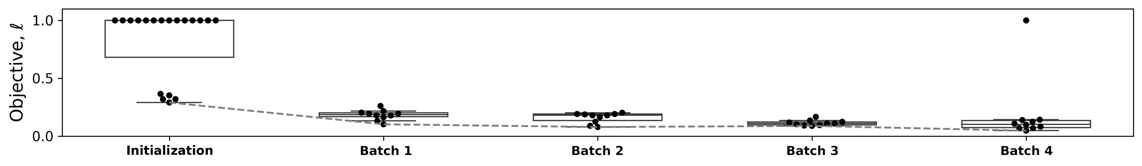
(d) Microfluidic MPI Objective Value per Batch

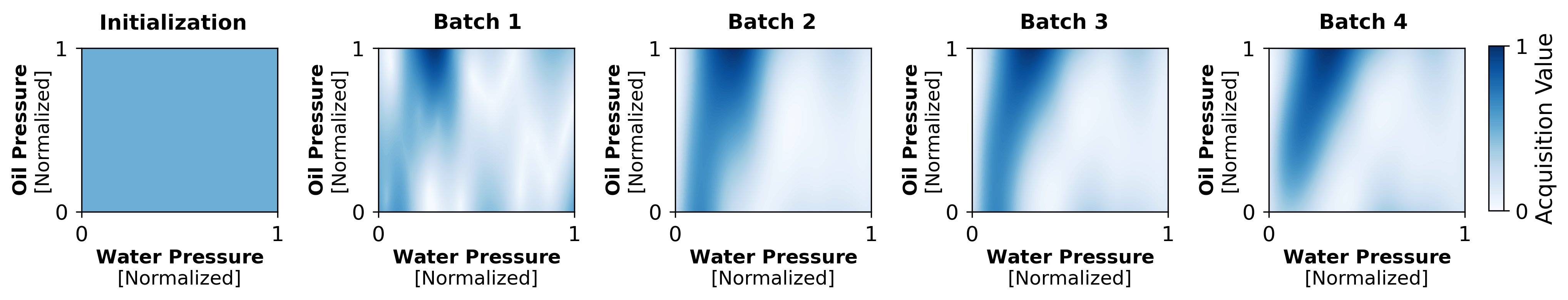
(e) Microfluidic LCB Acquisition Value per Batch

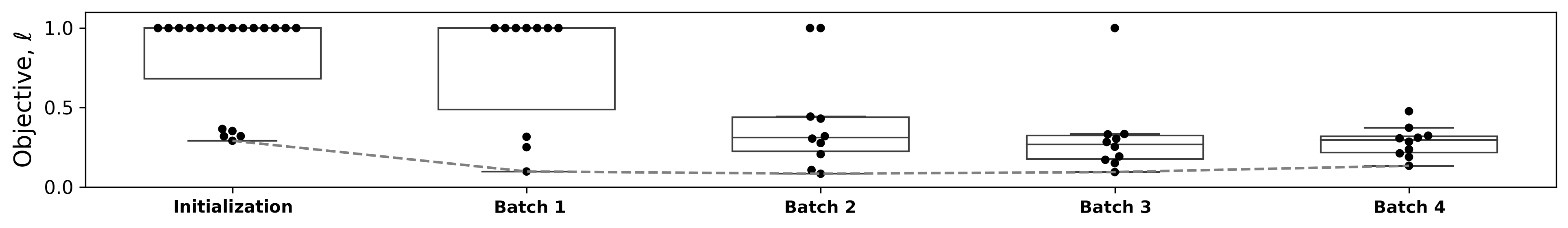
(f) Microfluidic LCB Objective Value per Batch

Figure S-3: Acquisition function search spaces by batch in 2-dimensions. The regions where each acquisition function is likely to draw points from within the microfluidic parameter space are illustrated in blue for each acquisition function: (a) EI, (c) MPI, (e) LCB – these denote regions of high acquisition value. The initialization acquisition space is a uniform color because points are picked uniformly during initialization via LHS. Based on the mechanics of each acquisition function, the acquisition value is computed by balancing the exploitation of the GP posterior mean and exploring the GP (co)variance. The acquisition search space evolves every loop, which updates the sampling locations of data points, shown for each acquisition function: (b) EI, (d) MPI, (f) LCB. The reason why the same data point that maximizes the acquisition value is not sampled 10 times for every batch in the loop is because of evaluator used is local penalization – points sampled close to each other are penalized, thus, the best point is selected first, then the second best (within some distance), and so on.

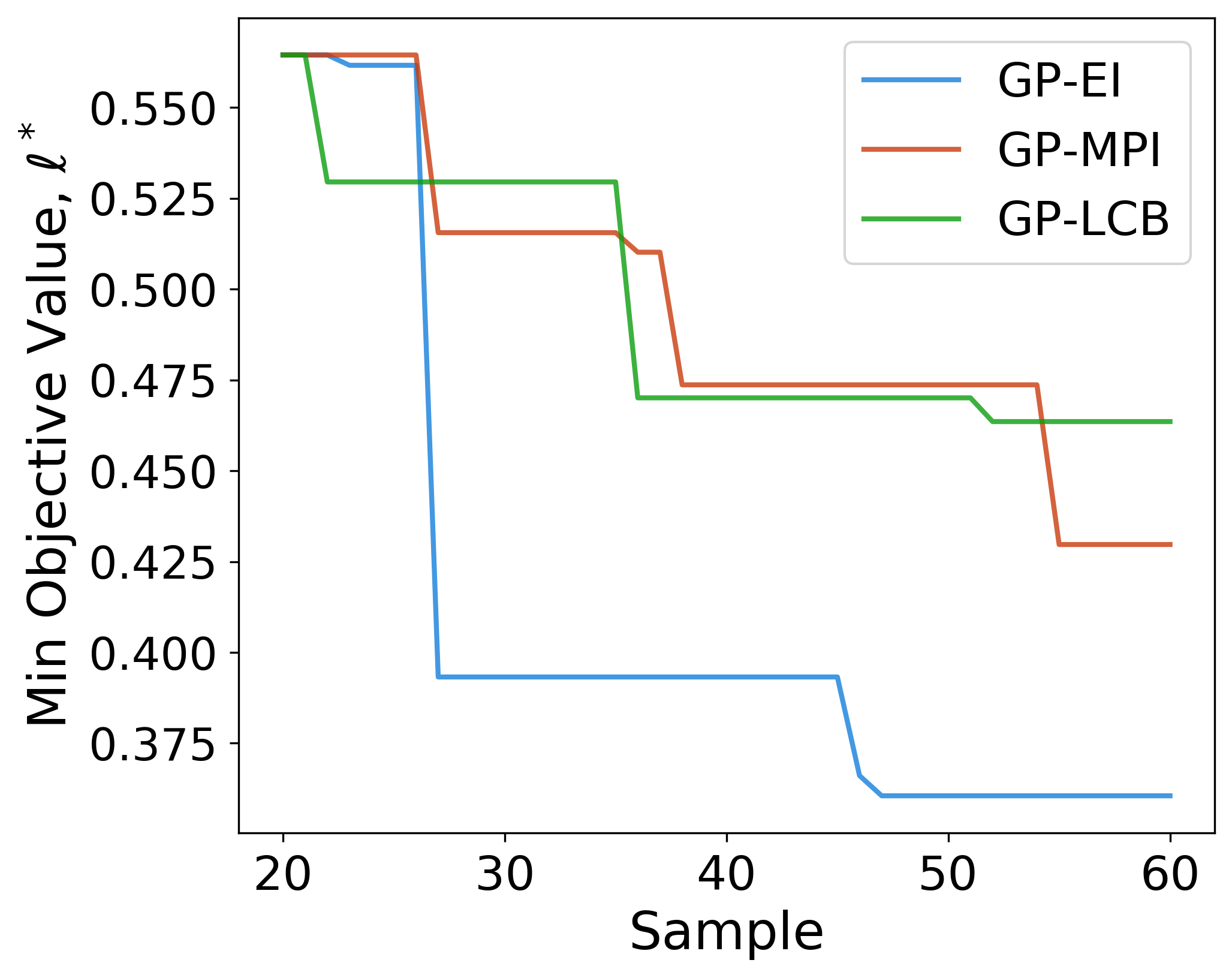
(a) Inkjet Running Best Objective Value, $\ell^{*}$

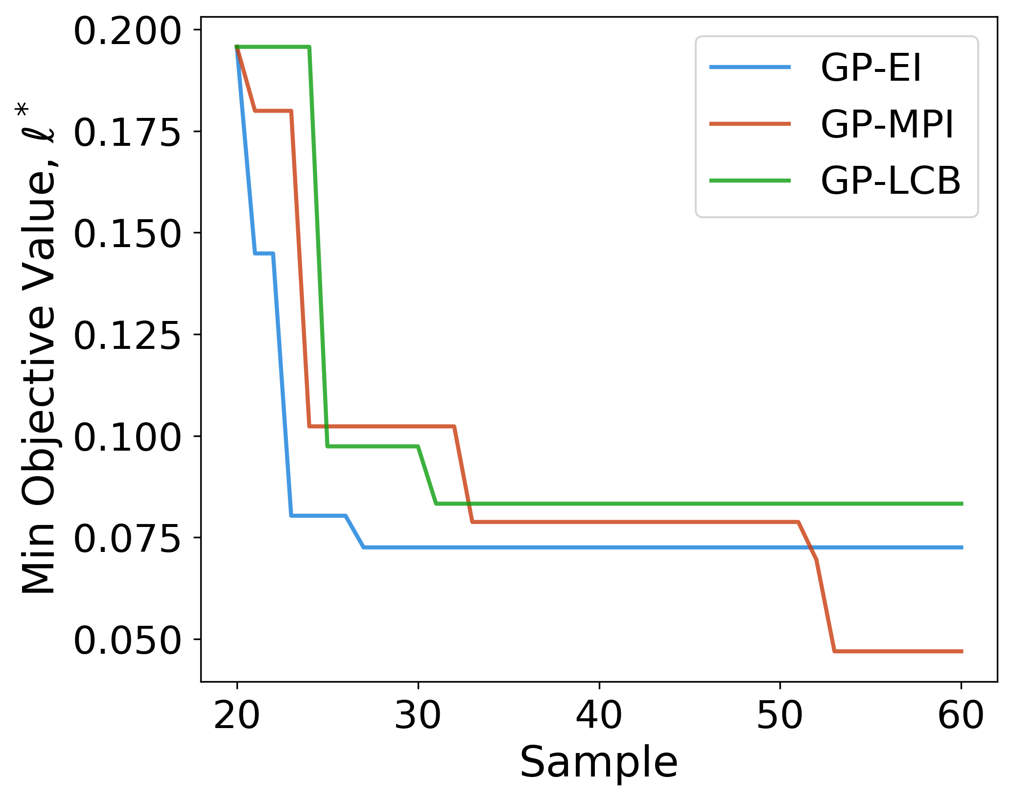
(b) Microfluidic Running Best Objective Value, $\ell^{*}$

Figure S-4: The running minimum objective function evaluation $\ell^{*}$ for (a) the inkjet device and (b) the microfluidic device. The optimum unstable fluid conditions that generate high yield and high uniformity droplets are labeled by $\ell^{*}\in[0,1]$ – the running minimum objective value. $\ell^{*}$ as a function of sample number is illustrated for each acquisition function after the 20 LHS initialization data points. The vertical axes are scaled differently for the inkjet and microfluidics devices, this scaling is arbitrary and is a result of the different droplet generating dynamics within each parameter space.

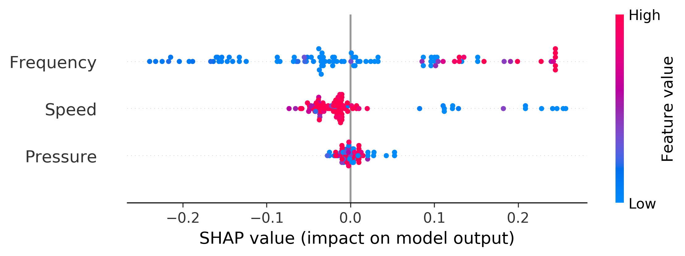
(a) Inkjet SHAP Feature Importance

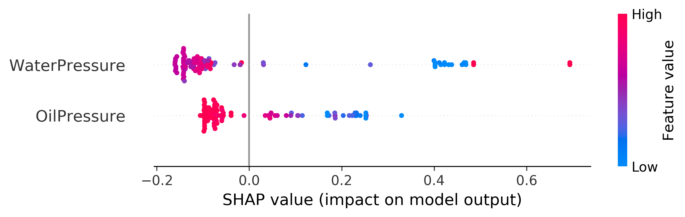
(b) Microfluidic SHAP Feature Importance

Figure S-5: The SHAP feature importance of the (a) inkjet and (b) microfluidic devices ⁴³. Random forest regression with an 80/20 training/test split is used to compute the SHAP feature importance of all acquisition function-sampled data. Each printing condition is shown to have a certain SHAP value – the magnitude of the SHAP value describes how much that condition impacts the objective values $\ell$. For example, low frequency values (blue) are shown to generate low $\ell$ values (high yield, uniform droplets), i.e., illustrated by high negative SHAP values; high frequency values (red) are shown to generate high $\ell$ values (low yield, not uniform droplets), i.e., illustrated by high positive SHAP values. High speed values have little impact on $\ell$, whereas low speed values generate high $\ell$ values. Pressure, in general, has little impact on $\ell$, shown by the clustering of all values of pressure conditions centered on a 0.0 SHAP value.

Table S-1: Inkjet conditions for three independent Bayesian experiments of droplet structures using three different decision policies: EI, MPI, LCB. The initialization dataset is obtained via LHS. This table details all of the experiments conducted for the Bayesian experimentation and optimization of droplet structures using the inkjet droplet deposition system. The synthesis conditions of $N=3$ control parameters: pressure, frequency, and speed, all reported as normalized values. The last column is the computer vision-computed loss, $\ell$, for each measurement.

Sample	Batch	Method	Pressure	Frequency	Speed	Loss
1	Initialization	LHS	0.583	0.719	0.002	1.000
2	Initialization	LHS	0.917	0.294	0.059	1.000
3	Initialization	LHS	0.667	0.552	0.118	1.000
4	Initialization	LHS	0.333	0.927	0.165	1.000
5	Initialization	LHS	0.083	0.169	0.226	1.000
6	Initialization	LHS	0.083	0.491	0.272	1.000
7	Initialization	LHS	0.167	0.660	0.312	1.000
8	Initialization	LHS	0.750	0.106	0.373	1.000
9	Initialization	LHS	0.250	0.303	0.443	0.717
10	Initialization	LHS	0.000	0.958	0.483	1.000
11	Initialization	LHS	0.500	0.500	0.520	0.720
12	Initialization	LHS	0.000	0.050	0.581	0.564
13	Initialization	LHS	0.750	0.036	0.608	0.630
14	Initialization	LHS	0.917	0.817	0.691	1.000
15	Initialization	LHS	0.417	0.377	0.704	0.728
16	Initialization	LHS	0.250	0.207	0.779	0.760
17	Initialization	LHS	0.667	0.423	0.811	0.678
18	Initialization	LHS	1.000	0.770	0.861	1.000
19	Initialization	LHS	0.000	0.638	0.930	1.000
20	Initialization	LHS	0.417	0.850	0.981	0.739
21	Batch 1	EI	0.000	0.000	1.000	1.000
22	Batch 1	EI	1.000	0.000	1.000	0.831
23	Batch 1	EI	0.333	0.065	0.996	0.562
24	Batch 1	EI	0.833	0.032	0.989	0.665
25	Batch 1	EI	0.000	0.090	0.992	0.567
26	Batch 1	EI	0.333	0.007	0.992	0.850
27	Batch 1	EI	0.833	0.109	0.972	0.393
28	Batch 1	EI	0.000	0.029	0.867	0.715
29	Batch 1	EI	0.833	0.013	0.985	0.715
30	Batch 1	EI	0.000	0.013	0.995	0.840
31	Batch 2	EI	0.833	0.000	1.000	0.812
32	Batch 2	EI	0.083	0.027	0.958	0.736
33	Batch 2	EI	1.000	0.076	0.969	0.603
34	Batch 2	EI	0.000	0.197	0.979	0.411
35	Batch 2	EI	0.083	0.009	1.000	0.833
36	Batch 2	EI	1.000	1.000	1.000	1.000
37	Batch 2	EI	1.000	0.000	1.000	0.829
38	Batch 2	EI	0.917	0.007	0.007	1.000
39	Batch 2	EI	0.000	0.009	0.119	0.521
40	Batch 2	EI	0.083	0.998	0.998	0.790
41	Batch 3	EI	1.000	0.201	1.000	0.685
42	Batch 3	EI	0.833	0.176	0.999	0.686
43	Batch 3	EI	1.000	0.223	0.970	0.673
44	Batch 3	EI	1.000	0.332	0.996	0.663
45	Batch 3	EI	0.833	0.192	0.990	0.685
46	Batch 3	EI	0.333	0.165	0.999	0.366
47	Batch 3	EI	0.583	0.147	1.000	0.361
48	Batch 3	EI	0.583	0.228	0.986	0.702
49	Batch 3	EI	0.750	0.149	0.995	0.368
50	Batch 3	EI	0.833	0.298	0.987	0.682
51	Batch 4	EI	0.000	0.147	1.000	0.460
52	Batch 4	EI	1.000	0.514	1.000	1.000
53	Batch 4	EI	0.167	0.143	1.000	0.449
54	Batch 4	EI	0.250	0.136	1.000	0.432
55	Batch 4	EI	0.000	0.447	1.000	0.809
56	Batch 4	EI	0.417	0.131	1.000	0.431
57	Batch 4	EI	0.250	0.482	1.000	0.767
58	Batch 4	EI	0.000	0.137	0.890	0.449
59	Batch 4	EI	0.250	0.145	0.954	0.434
60	Batch 4	EI	0.917	0.492	0.994	1.000
21	Batch 1	MPI	0.417	0.000	1.000	0.885
22	Batch 1	MPI	1.000	0.027	1.000	0.680
23	Batch 1	MPI	0.083	0.036	0.907	0.704
24	Batch 1	MPI	1.000	0.028	0.794	0.634
25	Batch 1	MPI	0.000	0.066	0.986	0.640
26	Batch 1	MPI	1.000	0.518	1.000	1.000
27	Batch 1	MPI	0.000	0.058	0.523	0.516
28	Batch 1	MPI	1.000	0.014	0.402	0.629
29	Batch 1	MPI	0.000	0.476	0.999	0.809
30	Batch 1	MPI	0.083	0.004	0.002	1.000
31	Batch 2	MPI	0.000	0.000	0.644	0.877
32	Batch 2	MPI	1.000	0.000	0.669	0.811
33	Batch 2	MPI	0.000	0.000	0.879	0.915
34	Batch 2	MPI	0.000	0.055	0.491	0.539
35	Batch 2	MPI	0.000	0.001	0.748	0.915
36	Batch 2	MPI	0.750	0.060	0.826	0.510
37	Batch 2	MPI	0.500	1.000	0.717	1.000
38	Batch 2	MPI	0.000	0.048	0.597	0.474
39	Batch 2	MPI	0.917	0.027	0.715	0.617
40	Batch 2	MPI	0.000	0.009	0.514	0.766
41	Batch 3	MPI	0.917	0.000	0.658	0.811
42	Batch 3	MPI	0.000	0.037	0.556	0.689
43	Batch 3	MPI	0.417	0.010	0.660	0.686
44	Batch 3	MPI	1.000	0.022	0.948	0.681
45	Batch 3	MPI	0.000	0.029	0.799	1.000
46	Batch 3	MPI	1.000	0.141	0.414	1.000
47	Batch 3	MPI	0.000	0.672	0.584	1.000
48	Batch 3	MPI	1.000	1.000	1.000	1.000
49	Batch 3	MPI	0.083	0.016	0.304	0.605
50	Batch 3	MPI	1.000	0.079	0.981	0.511
51	Batch 4	MPI	0.833	0.000	1.000	0.885
52	Batch 4	MPI	0.083	0.019	0.905	0.759
53	Batch 4	MPI	0.917	0.001	0.013	1.000
54	Batch 4	MPI	0.000	0.086	0.962	0.636
55	Batch 4	MPI	1.000	0.097	0.996	0.430
56	Batch 4	MPI	0.083	0.011	0.029	1.000
57	Batch 4	MPI	1.000	0.005	0.226	0.622
58	Batch 4	MPI	0.083	0.053	0.948	1.000
59	Batch 4	MPI	1.000	1.000	1.000	1.000
60	Batch 4	MPI	0.083	0.003	0.045	1.000
21	Batch 1	LCB	0.667	0.000	1.000	0.739
22	Batch 1	LCB	0.500	0.077	0.996	0.529
23	Batch 1	LCB	0.833	0.322	0.998	0.665
24	Batch 1	LCB	0.917	0.053	0.980	0.610
25	Batch 1	LCB	0.250	0.038	0.944	0.692
26	Batch 1	LCB	0.500	0.015	0.550	0.655
27	Batch 1	LCB	0.500	0.422	0.996	1.000
28	Batch 1	LCB	0.083	0.021	0.554	0.692
29	Batch 1	LCB	0.250	0.020	0.520	0.656
30	Batch 1	LCB	0.750	0.702	1.000	1.000
31	Batch 2	LCB	0.000	0.000	1.000	1.000
32	Batch 2	LCB	0.917	0.037	0.118	1.000
33	Batch 2	LCB	1.000	1.000	1.000	1.000
34	Batch 2	LCB	0.000	0.910	0.021	1.000
35	Batch 2	LCB	0.833	0.054	0.985	0.569
36	Batch 2	LCB	0.000	0.021	0.177	0.470
37	Batch 2	LCB	0.000	0.969	0.907	1.000
38	Batch 2	LCB	1.000	0.996	0.107	1.000
39	Batch 2	LCB	1.000	0.023	0.831	0.699
40	Batch 2	LCB	0.083	0.009	0.963	0.815
41	Batch 3	LCB	0.000	0.000	1.000	1.000
42	Batch 3	LCB	0.917	0.030	0.006	1.000
43	Batch 3	LCB	1.000	1.000	1.000	1.000
44	Batch 3	LCB	0.000	0.735	0.003	1.000
45	Batch 3	LCB	1.000	0.032	0.914	0.607
46	Batch 3	LCB	0.083	0.997	0.978	1.000
47	Batch 3	LCB	0.083	0.027	0.021	1.000
48	Batch 3	LCB	0.917	0.947	0.038	1.000
49	Batch 3	LCB	0.083	0.006	0.962	0.666
50	Batch 3	LCB	1.000	0.160	0.004	1.000
51	Batch 4	LCB	1.000	0.000	1.000	0.827
52	Batch 4	LCB	0.083	0.071	0.542	0.464
53	Batch 4	LCB	1.000	1.000	0.000	1.000
54	Batch 4	LCB	0.083	0.930	0.964	1.000
55	Batch 4	LCB	0.833	0.006	0.060	1.000
56	Batch 4	LCB	1.000	1.000	1.000	1.000
57	Batch 4	LCB	0.000	0.869	0.068	1.000
58	Batch 4	LCB	0.250	0.065	0.992	0.569
59	Batch 4	LCB	0.000	0.050	0.016	1.000
60	Batch 4	LCB	0.917	0.009	0.848	0.746

Table S-2: Microfluidics conditions for three independent Bayesian experiments of droplet structures using three different decision policies: EI, MPI, LCB. The initialization dataset is obtained via LHS. This table details all of the experiments conducted for the Bayesian experimentation and optimization of droplet structures using the microfluidic droplet deposition system. The synthesis conditions of $N=2$ control parameters: water pressure and oil pressure, all displayed as normalized values. The last column is the computer vision-computed loss, $\ell$, for each measurement.

Sample	Batch	Method	Water Pressure	Oil Pressure	Loss
1	Initialization	LHS	0.420	0.040	1.000
2	Initialization	LHS	0.043	0.083	0.352
3	Initialization	LHS	0.255	0.138	1.000
4	Initialization	LHS	0.727	0.168	1.000
5	Initialization	LHS	0.870	0.218	1.000
6	Initialization	LHS	0.155	0.277	0.365
7	Initialization	LHS	0.141	0.333	0.319
8	Initialization	LHS	0.812	0.399	1.000
9	Initialization	LHS	0.760	0.442	1.000
10	Initialization	LHS	0.948	0.465	1.000
11	Initialization	LHS	0.303	0.549	0.320
12	Initialization	LHS	0.208	0.599	0.291
13	Initialization	LHS	0.988	0.618	1.000
14	Initialization	LHS	0.575	0.674	1.000
15	Initialization	LHS	0.540	0.713	1.000
16	Initialization	LHS	0.648	0.796	1.000
17	Initialization	LHS	0.478	0.824	1.000
18	Initialization	LHS	0.068	0.887	1.000
19	Initialization	LHS	0.683	0.916	1.000
20	Initialization	LHS	0.392	0.979	0.196
21	Batch 1	EI	0.305	1.000	0.145
22	Batch 1	EI	0.321	0.987	0.157
23	Batch 1	EI	0.297	0.993	0.080
24	Batch 1	EI	0.315	0.949	0.176
25	Batch 1	EI	0.290	0.964	0.167
26	Batch 1	EI	0.302	0.915	0.188
27	Batch 1	EI	0.261	0.999	0.073
28	Batch 1	EI	0.330	0.992	0.186
29	Batch 1	EI	0.285	0.936	0.172
30	Batch 1	EI	0.294	0.881	0.194
31	Batch 2	EI	0.228	1.000	0.132
32	Batch 2	EI	0.219	0.989	0.137
33	Batch 2	EI	0.214	0.924	0.134
34	Batch 2	EI	0.203	0.997	0.201
35	Batch 2	EI	0.227	0.948	0.168
36	Batch 2	EI	1.000	0.000	1.000
37	Batch 2	EI	0.176	0.995	0.242
38	Batch 2	EI	0.243	0.987	0.170
39	Batch 2	EI	0.202	0.899	0.168
40	Batch 2	EI	0.260	0.995	0.131
41	Batch 3	EI	0.261	1.000	0.090
42	Batch 3	EI	0.260	0.977	0.115
43	Batch 3	EI	0.272	0.999	0.105
44	Batch 3	EI	0.099	0.000	1.000
45	Batch 3	EI	0.002	0.000	1.000
46	Batch 3	EI	0.251	0.992	0.111
47	Batch 3	EI	0.879	1.000	1.000
48	Batch 3	EI	0.254	0.987	0.097
49	Batch 3	EI	0.258	0.935	0.153
50	Batch 3	EI	0.270	0.960	0.151
51	Batch 4	EI	0.000	0.252	1.000
52	Batch 4	EI	0.009	0.234	1.000
53	Batch 4	EI	0.019	0.316	1.000
54	Batch 4	EI	0.031	0.188	0.971
55	Batch 4	EI	0.005	0.372	1.000
56	Batch 4	EI	0.003	0.296	1.000
57	Batch 4	EI	0.030	0.199	1.000
58	Batch 4	EI	0.001	0.197	1.000
59	Batch 4	EI	0.049	0.251	0.483
60	Batch 4	EI	0.003	0.166	1.000
21	Batch 1	MPI	0.382	0.989	0.180
22	Batch 1	MPI	0.360	0.947	0.194
23	Batch 1	MPI	0.327	0.886	0.194
24	Batch 1	MPI	0.332	0.996	0.102
25	Batch 1	MPI	0.316	0.818	0.216
26	Batch 1	MPI	0.316	0.938	0.163
27	Batch 1	MPI	0.316	0.744	0.261
28	Batch 1	MPI	0.281	0.861	0.178
29	Batch 1	MPI	0.371	0.922	0.203
30	Batch 1	MPI	0.295	0.995	0.132
31	Batch 2	MPI	0.335	1.000	0.188
32	Batch 2	MPI	0.334	0.979	0.180
33	Batch 2	MPI	0.291	0.997	0.079
34	Batch 2	MPI	0.313	0.994	0.180
35	Batch 2	MPI	0.266	0.982	0.089
36	Batch 2	MPI	0.324	0.999	0.191
37	Batch 2	MPI	0.325	0.998	0.125
38	Batch 2	MPI	0.357	0.987	0.202
39	Batch 2	MPI	0.356	0.993	0.191
40	Batch 2	MPI	0.228	0.998	0.164
41	Batch 3	MPI	0.268	1.000	0.095
42	Batch 3	MPI	0.246	0.962	0.091
43	Batch 3	MPI	0.281	0.999	0.088
44	Batch 3	MPI	0.270	0.953	0.109
45	Batch 3	MPI	0.279	0.967	0.118
46	Batch 3	MPI	0.260	0.921	0.166
47	Batch 3	MPI	0.261	0.989	0.103
48	Batch 3	MPI	0.289	0.992	0.123
49	Batch 3	MPI	0.260	0.969	0.110
50	Batch 3	MPI	0.253	0.890	0.135
51	Batch 4	MPI	0.265	1.000	0.107
52	Batch 4	MPI	0.276	1.000	0.070
53	Batch 4	MPI	0.276	0.989	0.047
54	Batch 4	MPI	0.274	0.974	0.082
55	Batch 4	MPI	0.262	1.000	0.097
56	Batch 4	MPI	0.253	0.957	0.139
57	Batch 4	MPI	0.000	0.000	1.000
58	Batch 4	MPI	0.252	0.980	0.124
59	Batch 4	MPI	0.257	0.986	0.069
60	Batch 4	MPI	0.268	0.952	0.141
21	Batch 1	LCB	1.000	0.000	1.000
22	Batch 1	LCB	0.000	0.503	1.000
23	Batch 1	LCB	0.000	0.280	1.000
24	Batch 1	LCB	0.000	0.000	1.000
25	Batch 1	LCB	0.254	1.000	0.097
26	Batch 1	LCB	0.001	0.172	1.000
27	Batch 1	LCB	1.000	1.000	1.000
28	Batch 1	LCB	0.142	0.495	0.316
29	Batch 1	LCB	0.006	0.639	1.000
30	Batch 1	LCB	0.452	1.000	0.250
31	Batch 2	LCB	0.301	1.000	0.083
32	Batch 2	LCB	0.277	0.846	0.107
33	Batch 2	LCB	0.226	0.661	0.276
34	Batch 2	LCB	0.161	0.997	0.430
35	Batch 2	LCB	0.000	0.125	1.000
36	Batch 2	LCB	0.178	0.428	0.319
37	Batch 2	LCB	0.373	0.950	0.207
38	Batch 2	LCB	0.149	0.204	0.443
39	Batch 2	LCB	0.367	0.761	0.304
40	Batch 2	LCB	0.335	0.534	1.000
41	Batch 3	LCB	0.298	1.000	0.150
42	Batch 3	LCB	0.246	0.875	0.094
43	Batch 3	LCB	0.225	0.724	0.253
44	Batch 3	LCB	0.394	0.991	0.192
45	Batch 3	LCB	0.180	0.522	0.303
46	Batch 3	LCB	0.195	0.993	0.283
47	Batch 3	LCB	0.133	0.294	0.333
48	Batch 3	LCB	0.121	0.000	1.000
49	Batch 3	LCB	0.358	0.841	0.171
50	Batch 3	LCB	0.303	0.607	0.331
51	Batch 4	LCB	0.307	1.000	0.133
52	Batch 4	LCB	0.264	0.812	0.236
53	Batch 4	LCB	0.192	0.619	0.285
54	Batch 4	LCB	0.216	0.993	0.189
55	Batch 4	LCB	0.165	0.422	0.323
56	Batch 4	LCB	0.431	0.999	0.310
57	Batch 4	LCB	0.321	0.695	0.306
58	Batch 4	LCB	0.141	0.250	0.373
59	Batch 4	LCB	0.332	0.895	0.212
60	Batch 4	LCB	0.141	0.807	0.477

References

- Song et al. 2020 Song, M.; Kartawira, K.; Hillaire, K. D.; Li, C.; Eaker, C. B.; Kiani, A.; Daniels, K. E.; Dickey, M. D. Overcoming Rayleigh–Plateau Instabilities: Stabilizing and Destabilizing Liquid-metal Streams via Electrochemical Oxidation. Proceedings of the National Academy of Sciences 2020, 117, 19026–19032
- Papageorgiou 1995 Papageorgiou, D. T. On the Breakup of Viscous Liquid Threads. Physics of Fluids 1995, 7, 1529–1544
- Gu et al. 2011 Gu, H.; Duits, M. H.; Mugele, F. Droplets Formation and Merging in Two-phase Flow Microfluidics. International Journal of molecular sciences 2011, 12, 2572–2597
- Mei 2004 Mei, C. C. Advanced Fluid Mechanics; Massachusetts Institute of Technology, 2004
- Anna and Mayer 2006 Anna, S. L.; Mayer, H. C. Microscale Tipstreaming in a Microfluidic Flow Focusing Device. Physics of Fluids 2006, 18, 121512
- Derby 2011 Derby, B. Inkjet Printing Ceramics: From Drops to Solid. Journal of the European Ceramic Society 2011, 31, 2543–2550
- Chu et al. 2019 Chu, A. B.; Nguyen, D. T.; Kaplan, A. D.; Giera, B. Image Classification and Control of Microfluidic Systems. Applications of Machine Learning. 2019; p 3
- Miller et al. 2010 Miller, E.; Rotea, M.; Rothstein, J. P. Microfluidic Device Incorporating Closed Loop Feedback Control for Uniform and Tunable Production of Micro-droplets. Lab on a Chip 2010, 10, 1293–1301
- Drugowitsch et al. 2019 Drugowitsch, J.; Mendonça, A. G.; Mainen, Z. F.; Pouget, A. Learning Optimal Decisions with Confidence. Proceedings of the National Academy of Sciences 2019, 116, 24872–24880
- Barnes et al. 2011 Barnes, C. P.; Silk, D.; Sheng, X.; Stumpf, M. P. H. Bayesian Design of Synthetic Biological Systems. Proceedings of the National Academy of Sciences 2011, 108, 15190–15195
- Hennig and Schuler 2012 Hennig, P.; Schuler, C. J. Entropy Search for Information-efficient Global Optimization. Journal of Machine Learning Research 2012, 13, 1809–1837
- Seeger 2004 Seeger, M. Gaussian Processes for Machine Learning. International journal of neural systems 2004, 14, 69–106
- Ohnesorge 2019 Ohnesorge, W. v. The Formation of Drops by Nozzles and the Breakup of Liquid Jets. 2019
- Baroud et al. 2010 Baroud, C. N.; Gallaire, F.; Dangla, R. Dynamics of Microfluidic Droplets. Lab on a Chip 2010, 10, 2032–2045
- Bash et al. 2020 Bash, D.; Yongqiang, C.; Chellappan, V.; Liang, W. S.; Yang, X.; Kumar, P.; Da, T. J.; Abutaha, A.; Cheng, J.; Yee-Fun, L.; Tian, S.; Ren, D. Z.; Mekki-Barrada, F.; Wong, W. K.; Kumar, J.; Khan, S.; Qianxiao, L.; Buonassisi, T.; Hippalgaonkar, K. Machine Learning and High-throughput Robust Design of P3HT-CNT Composite Thin Films for High Electrical Conductivity. ChemRxiv 2020,
- Langner et al. 2020 Langner, S.; Häse, F.; Perea, J. D.; Stubhan, T.; Hauch, J.; Roch, L. M.; Heumueller, T.; Aspuru-Guzik, A.; Brabec, C. J. Beyond Ternary OPV: High-Throughput Experimentation and Self-Driving Laboratories Optimize Multicomponent Systems. Advanced Materials 2020, 32
- Sun et al. 2019 Sun, S.; Hartono, N. T.; Ren, Z. D.; Oviedo, F.; Buscemi, A. M.; Layurova, M.; Chen, D. X.; Ogunfunmi, T.; Thapa, J.; Ramasamy, S.; Settens, C.; DeCost, B. L.; Kusne, A. G.; Liu, Z.; Tian, S. I.; Peters, I. M.; Correa-Baena, J. P.; Buonassisi, T. Accelerated Development of Perovskite-Inspired Materials via High-Throughput Synthesis and Machine-Learning Diagnosis. Joule 2019, 3, 1437–1451
- Sun et al. 2021 Sun, S.; Tiihonen, A.; Oviedo, F.; Liu, Z.; Thapa, J.; Zhao, Y.; Hartono, N. T. P.; Goyal, A.; Heumueller, T.; Batali, C.; Encinas, A.; Yoo, J. J.; Li, R.; Ren, Z.; Peters, I. M.; Brabec, C. J.; Bawendi, M. G.; Stevanovic, V.; Fisher, J.; Buonassisi, T. A Data Fusion Approach to Optimize Compositional Stability of Halide Perovskites. Matter 2021, 4
- Ren et al. 2020 Ren, Z.; Oviedo, F.; Thway, M.; Tian, S. I.; Wang, Y.; Xue, H.; Dario Perea, J.; Layurova, M.; Heumueller, T.; Birgersson, E.; Aberle, A. G.; Brabec, C. J.; Stangl, R.; Li, Q.; Sun, S.; Lin, F.; Peters, I. M.; Buonassisi, T. Embedding Physics Domain Knowledge into a Bayesian Network Enables Layer-by-layer Process Innovation for Photovoltaics. npj Computational Materials 2020, 6, 1–9
- Fridman et al. 2021 Fridman, I. B.; Ugolini, G. S.; VanDelinder, V.; Cohen, S.; Konry, T. High Throughput Microfluidic System with Multiple Oxygen Levels for the Study of Hypoxia in Tumor Spheroids. Biofabrication 2021, 13, 035037
- Ding et al. 2019 Ding, Y.; Howes, P. D.; deMello, A. J. Recent Advances in Droplet Microfluidics. Analytical chemistry 2019, 92, 132–149
- Shang et al. 2017 Shang, L.; Cheng, Y.; Zhao, Y. Emerging Droplet Microfluidics. Chemical reviews 2017, 117, 7964–8040
- Kaufman et al. 2015 Kaufman, G.; Nejati, S.; Sarfati, R.; Boltyanskiy, R.; Loewenberg, M.; Dufresne, E. R.; Osuji, C. O. Soft Microcapsules with Highly Plastic Shells Formed by Interfacial Polyelectrolyte–nanoparticle Complexation. Soft Matter 2015, 11, 7478–7482
- Bah et al. 2020 Bah, M. G.; Bilal, H. M.; Wang, J. Fabrication and Application of Complex Microcapsules: A Review. Soft Matter 2020, 16, 570–590
- Huang et al. 2017 Huang, H.; Yu, Y.; Hu, Y.; He, X.; Usta, O. B.; Yarmush, M. L. Generation and Manipulation of Hydrogel Microcapsules by Droplet-based Microfluidics for Mammalian Cell Culture. Lab on a Chip 2017, 17, 1913–1932
- Sesen et al. 2017 Sesen, M.; Alan, T.; Neild, A. Droplet Control Technologies for Microfluidic High Throughput Screening (HTS). Lab on a Chip 2017, 17, 2372–2394
- Joanicot and Ajdari 2005 Joanicot, M.; Ajdari, A. Droplet Control for Microfluidics. Science 2005, 309, 887–888
- Lashkaripour et al. 2021 Lashkaripour, A.; Rodriguez, C.; Mehdipour, N.; Mardian, R.; McIntyre, D.; Ortiz, L.; Campbell, J.; Densmore, D. Machine Learning Enables Design Automation of Microfluidic Flow-focusing Droplet Generation. Nature communications 2021, 12, 1–14
- McKinley and Renardy 2011 McKinley, G. H.; Renardy, M. Wolfgang von Ohnesorge. Physics of Fluids 2011, 23, 127101
- Clanet and Lasheras 1999 Clanet, C.; Lasheras, J. C. Transition from Dripping to Jetting. Journal of Fluid Mechanics 1999, 383, 307–326
- Tai et al. 2008 Tai, J.; Gan, H. Y.; Liang, Y. N.; Lok, B. K. Control of Droplet Formation in Inkjet Printing Using Ohnesorge Number Category: Materials and Processes. 2008 10th Electronics Packaging Technology Conference. 2008; pp 761–766
- Utada et al. 2007 Utada, A. S.; Fernandez-Nieves, A.; Stone, H. A.; Weitz, D. A. Dripping to Jetting Transitions in Coflowing Liquid Streams. Physical review letters 2007, 99, 094502
- Lignel et al. 2017 Lignel, S.; Salsac, A.-V.; Drelich, A.; Leclerc, E.; Pezron, I. Water-in-oil Droplet Formation in a Flow-focusing Microsystem using Pressure and Flow Rate-driven Pumps. Colloids and Surfaces A: Physicochemical and Engineering Aspects 2017, 531, 164–172
- Jeyhani et al. 2019 Jeyhani, M.; Gnyawali, V.; Abbasi, N.; Hwang, D. K.; Tsai, S. S. Microneedle-assisted Microfluidic Flow Focusing for Versatile and High Throughput Water-in-water Droplet Generation. Journal of colloid and interface science 2019, 553, 382–389
- Cubaud and Mason 2008 Cubaud, T.; Mason, T. G. Capillary Threads and Viscous Droplets in Square Microchannels. Physics of fluids 2008, 20, 053302
- Garstecki et al. 2005 Garstecki, P.; Stone, H. A.; Whitesides, G. M. Mechanism for Flow-rate Controlled Breakup in Confined Geometries a Route to Monodisperse emulsions. Physical review letters 2005, 94, 164501
- McKay et al. 2000 McKay, M. D.; Beckman, R. J.; Conover, W. J. A comparison of three methods for selecting values of input variables in the analysis of output from a computer code. Technometrics 2000, 42, 55–61
- Itseez 2021 Itseez, OpenCV: Image Segmentation with Watershed Algorithm. https://docs.opencv.org/master/d3/db4/tutorial_py_watershed.html, 2021; https://docs.opencv.org/master/d3/db4/tutorial_py_watershed.html
- Gatys et al. 2015 Gatys, L. A.; Ecker, A. S.; Bethge, M. A Neural Algorithm of Artistic Style. arXiv 2015,
- GPy since 2012 GPy, GPy: A Gaussian Process Framework in Python. http://github.com/SheffieldML/GPy, since 2012
- Brochu et al. 2010 Brochu, E.; Cora, V. M.; de Freitas, N. A Tutorial on Bayesian Optimization of Expensive Cost Functions, with Application to Active User Modeling and Hierarchical Reinforcement Learning. arXiv:1012.2599 2010,
- Sommers and Jacobi 2008 Sommers, A.; Jacobi, A. M. Calculating the Volume of Water Droplets on Aluminum Surfaces. International Refrigeration and Air Conditioning Conference 2008, 1–8
- Lundberg and Lee 2017 Lundberg, S. M.; Lee, S.-I. Advances in Neural Information Processing Systems 30; Curran Associates, Inc., 2017; pp 4765–4774
- Derby 2010 Derby, B. Inkjet Printing of Functional and Structural Materials: Fluid Property Requirements, Feature Stability, and Resolution. Annual Review of Materials Research 2010, 40, 395–414
- Eggers and Villermaux 2008 Eggers, J.; Villermaux, E. Physics of Liquid Jets. Reports on Progress in Physics 2008, 71, 036601