Dark Energy Survey Year 3 Results: Multi-Probe Modeling Strategy and Validation

Abstract

This paper details the modeling pipeline and validates the baseline analysis choices of the DES Year 3 joint analysis of galaxy clustering and weak lensing (a so-called “3$\times$2pt” analysis). These analysis choices include the specific combination of cosmological probes, priors on cosmological and systematics parameters, model parameterizations for systematic effects and related approximations, and angular scales where the model assumptions are validated. We run a large number of simulated likelihood analyses using synthetic data vectors to test the robustness of our baseline analysis. We demonstrate that the DES Year 3 modeling pipeline, including the calibrated scale cuts, is sufficiently accurate relative to the constraining power of the DES Year 3 analyses. Our systematics mitigation strategy accounts for astrophysical systematics, such as galaxy bias, intrinsic alignments, source and lens magnification, baryonic effects, and source clustering, as well as for uncertainties in modeling the matter power spectrum, reduced shear, and estimator effects. We further demonstrate excellent agreement between two independently-developed modeling pipelines, and thus rule out any residual uncertainties due to the numerical implementation.

I Introduction

Photometric wide-field imaging surveys, such as the Dark Energy Survey (DES), Hyper Suprime Cam Subaru Strategic Project (HSC), and the Kilo-Degree Survey (KiDS) have published exciting results constraining the geometry and structure growth of the Universe (Abbott et al., 2018; Hamana et al., 2020; Heymans et al., 2021). These results are leading up to data sets with ever increasing statistical precision that are due to arrive in the mid 2020s from Rubin Observatory’s Legacy Survey of Space and Time (LSST), the Euclid satellite, and the Roman Space Telescope. The statistical precision of the data must be matched by the modeling accuracy on the analysis side, lest cosmological constraints incur substantial systematic bias.

This paper is part of a series describing the methodology and results of DES Year 3 (Y3) analysis, which combines cosmic shear, galaxy-galaxy lensing and galaxy clustering measurements (together termed a 3$\times$2pt analysis) from photometric date covering more than 4,000 square degrees, corresponding to the first 50% of the complete DES data set. Our papers present cosmological constraints for cosmic shear (Amon et al., 2021; Secco et al., 2021), the combination of galaxy clustering (Rodríguez-Monroy et al., 2021) and galaxy-galaxy lensing (Prat et al., 2021), termed 2$\times$2pt analysis, using two different lens galaxy samples (Pandey et al., 2021; Porredon et al., 2021), as well as the 3$\times$2pt analysis (DES Collaboration, 2021). These cosmological results are enabled by extensive methodology developments at all stages of the analysis; see Appendix A of Ref. (DES Collaboration, 2021) for a summary.

While there is extensive literature characterizing the impact of different systematic effects on future surveys in isolation, data analyses require all relevant systematic effects to be identified, modeled and mitigated in combination. The corresponding analysis choices, which encompass probes, choice of angular scales analyzed and redshift binning of the measurements/data, choice of parameterizations, and choice of parameter priors, are highly survey- and analysis-specific (e.g., Krause et al., 2017; Joachimi et al., 2021). This paper motivates and validates the theoretical modeling and analysis choices for the DES-Y3 cosmic shear, 2$\times$2pt and 3$\times$2pt analyses. We systematically define astrophysical and cosmological modeling choices, and demonstrate the robustness of our adopted baseline parameterization through simulated likelihood analyses. The resulting model parameterization, analysis choices, and inference pipeline are further validated through analyses of detailed DES mock catalogs (DeRose et al., 2019), which are presented in DeRose et al. (2021). We note that the DES-Y3 analysis was blinded to minimize experimenter bias, and the modeling and analysis choices in this paper were finalized before unblinding. We refer to DES Collaboration (2021) for a description of the blinding protocol and post-unblinding analysis choices.

In order to identify modeling choices as comprehensively as possible, we first summarize the theoretical formalism for calculating angular 3$\times$2pt statistics, avoiding specific model choices to the extent possible, in Sect. II. In Sect. III we then motivate modeling choices required to evaluate the general expressions for 3$\times$2pt statistics, which are summarized in Table 1. While each of the systematics identified in Table 1 has been studied extensively in isolation before, such principled approaches to identifying relevant systematics will become especially useful with increasing model complexity. We validate the robustness of the assumed scale dependence and redshift dependence of each systematic parameterization through model stress tests in the form of simulated likelihood analyses (described in Sect. IV). These stress tests are detailed in Sect. V and summarized in Table 1. Our conclusions are presented in Sect. VI.

II Formalism

In this section we derive the theoretical formalism for computing angular 3$\times$2pt statistics, assuming general relativity, a spatially flat universe, and working to leading order in the lensing distortion. The astrophysical model choices required to evaluate these expressions will be specified in Sect. III, and we specify the galaxy samples corresponding to the DESY3 analysis in Sect. IV.

We use lower-case, italic-type superscripts ($i,j$) to indicate tomograpic bin indices, and lower-case Greek subscripts for vector and shear components on the flat sky with respect to the Cartesian coordinate system (e.g., $\alpha=1,2$). Lower-case roman subscripts are used to denote specific galaxy samples ($\mathrm{s}$ for the source galaxy sample, $\mathrm{l}$ for the lens galaxy sample), while the lower-case italic subscript $g$ is used for a generic galaxy sample, $g\in(\mathrm{l},\mathrm{s})$. When specifying the type of correlation function or power spectrum, we use upper-case cursive subscripts to denote a generic tracer field, e.g., $\mathcal{A,B}\in(\kappa,\delta_{\mathrm{m}},\delta_{g},B,E,\mathrm{I}_{E},\mathrm{I}_{B}$). For ease of notation, we refer to angular bins by a representative separation $\theta$, but note that all correlation functions are averaged over angular bins $\left[\theta_{\mathrm{min}},\theta_{\mathrm{max}}\right]$ (c.f. Eq. 20).

II.1 Field-Level Description

The DES-Y3 3$\times$2pt analysis is based on the cross-correlation functions of the observed projected galaxy density contrast of the lens sample, $\delta_{\mathrm{l}}^{i}$, and shear, $\gamma_{\alpha}^{j}$, in tomographic redshift bins $i$ and $j$ of the lens and source galaxy sample respectively. We use $n_{g}^{i}(z)$ to denote the normalized tomographic redshift distribution of galaxy samples.

II.1.1 Galaxy density

The observed projected galaxy density contrast $\delta_{g,\mathrm{obs}}^{i}(\hat{\mathbf{n}})$ of galaxies from sample $g$ and tomographic bin $i$ at position $\hat{\mathbf{n}}$ can be written as

$$\delta_{g,\mathrm{obs}}^{i}(\hat{\mathbf{n}})= \underbrace{\int d\chi\,W^{i}_{\delta,g}\left(\chi\right)\delta_{g}^{(\rm 3D)}\left(\hat{\mathbf{n}}\chi,\chi\right)}_{\delta_{g,\mathrm{D}}^{i}(\hat{\mathbf{n}})}$$

$$+\delta_{g,\mathrm{RSD}}^{i}(\hat{\mathbf{n}})+\delta_{g,\mu}^{i}(\hat{\mathbf{n}})\,,$$ (1)

with $\chi$ the comoving distance, and $W_{\delta,g}^{i}=n_{g}^{i}(z)\,dz/d\chi$ the normalized selection function of galaxies in tomographic bin $i$. Here the first term ($\delta_{g,\mathrm{D}}$) is the line-of-sight projection of the three-dimensional galaxy density contrast, $\delta_{g}^{(\rm 3D)}$, of sample $g$, and the remaining terms are the contributions from linear redshift space distortions (RSD) and magnification ($\mu$).

In the linear regime, RSD contribute to the projected galaxy density contrast through the apparent large-scale flow, with velocity $\mathbf{v}$, of galaxies across the redshift boundaries of the tomographic bins, which can be modeled as (Fisher et al., 1994; Padmanabhan et al., 2007)

$$\delta_{g,\mathrm{obs}}^{i}(\hat{\mathbf{n}})= \!\int\!d\chi\,W^{i}_{\delta,g}\left(\chi\!+\!\hat{\mathbf{n}}\!\cdot\!\mathbf{v}(\hat{\mathbf{n}}\chi,\chi)\right)\!\left[1+\delta_{g}^{(\rm 3D)}\!\left(\hat{\mathbf{n}}\chi,\chi\right)\right]-1$$

$$\;+\delta_{g,\mu}^{i}(\hat{\mathbf{n}})$$

$$\approx \delta_{g,\mathrm{D}}^{i}(\hat{\mathbf{n}})-\!\!\int\!d\chi\,W^{i}_{\delta,g}\!\left(\chi\right)\frac{\partial}{\partial\chi}\!\left(\frac{\hat{\mathbf{n}}\!\cdot\!\mathbf{v}(\hat{\mathbf{n}}\chi,\chi)}{a(\chi)H(\chi)}\!\right)+\delta_{g,\mu}^{i}(\hat{\mathbf{n}})\,,$$

with $a$ the scale factor, and $H(\chi)$ the Hubble rate at redshift $z(\chi)$.

The magnification term describes the change in projected number density due to geometric dilution as well as magnification effects on galaxy flux (Verner Villumsen, 1995; Moessner and Jain, 1998) and size (Schmidt et al., 2009a), which modulate the selection function. The magnitude of the latter two effects depends on the flux and size distribution of the galaxy sample, and we introduce the proportionality constant $C_{g}^{i}$ to write the magnification term as

$$\delta_{g,\mu}^{i}(\hat{\mathbf{n}})=C_{g}^{i}\kappa_{g}^{i}(\hat{\mathbf{n}})\,$$ (3)

where we have introduced the tomographic convergence field

$$\kappa_{g}^{i}(\hat{\mathbf{n}})=\int d\chi\,W_{\kappa,g}^{i}(\chi)\delta_{\mathrm{m}}\left(\hat{\mathbf{n}}\chi,\chi\right)$$ (4)

with $\delta_{\mathrm{m}}$ the 3D matter density contrast, and the tomographic lens efficiency

$$W_{\kappa,g}^{i}(\chi)=\frac{3\Omega_{\rm m}H_{0}^{2}}{2c^{2}}\int_{\chi}^{\infty}d\chi^{\prime}n_{g}^{i}(\chi^{\prime})\frac{\chi}{a(\chi)}\frac{\chi^{\prime}-\chi}{\chi^{\prime}}\,.$$ (5)

II.1.2 Weak Lensing

The two components $\gamma_{\alpha}$ of the observed galaxy shapes are modeled as gravitational shear ($\mathrm{G}$) and intrinsic ellipticity. The latter is split into a spatially-coherent contribution from intrinsic galaxy alignments (IA), and stochastic shape noise $\epsilon_{0}$

$$\gamma_{\alpha}^{j}(\hat{\mathbf{n}})=\gamma_{\alpha,\mathrm{G}}^{j}(\hat{\mathbf{n}})+\gamma_{\alpha,\mathrm{IA}}^{j}(\hat{\mathbf{n}})+\epsilon_{\alpha,0}^{j}(\hat{\mathbf{n}})\,.$$ (6)

As shape noise contributes to the covariance but not to the mean two-point correlation function signal, we do not include it in the mean model predictions described here and defer to Amon et al. (2021); Friedrich et al. (2020) for details on the covariance modeling.

The gravitational shear can be calculated as

$$\gamma_{1,\mathrm{G}}=\left(\Psi_{11}-\Psi_{22}\right)/2\,,\;\gamma_{2,\mathrm{G}}=\left(\Psi_{12}+\Psi_{21}\right)/2\,,$$ (7)

with $\Psi$ the lensing distortion tensor, which to leading order in the lensing deflection can be calculated as

$$\Psi_{\alpha\beta}^{i}(\hat{\mathbf{n}})=2\int d\chi W_{\kappa,\mathrm{s}}^{i}(\chi)\,\chi\,\Phi_{,\alpha\beta}(\hat{\mathbf{n}}\chi,\chi)\,.$$ (8)

Here $\Phi_{,\alpha}$ are spatial transverse derivatives of the 3D potential $\Phi$.

Again to leading order in the lensing deflection, in Fourier space the gravitational shear field with respect to the Cartesian coordinate system can be related to the convergence $\kappa_{s}^{i}$ by

$$\gamma^{i}_{\alpha,\mathrm{G}}(\bm{\ell})=T_{\alpha}(\bm{\ell})\kappa_{\mathrm{s}}^{i}(\bm{\ell})\,,$$ (9)

with $\mathbf{T}(\bm{\ell})\equiv(\cos(2\phi_{\ell}),\sin(2\phi_{\ell}))$, where $\phi_{\ell}$ is the angle of the $\bm{\ell}$ vector from the $\ell_{x}$ axis.

The intrinsic alignment contribution to the observed galaxy shear field is a projection of the 3D field $\tilde{\gamma}_{\mathrm{IA}}$ weighted by the source galaxy redshift distribution

$$\gamma_{\alpha,\mathrm{IA}}^{i}(\hat{\mathbf{n}})=\int d\chi\,W_{\delta,\rm{s}}^{i}(\chi)\tilde{\gamma}_{\alpha,\mathrm{IA}}\left(\hat{\mathbf{n}}\chi,\chi\right)\,.$$ (10)

The 3D intrinsic alignment field, $\tilde{\gamma}_{\mathrm{IA}}$, is specified by the choice of intrinsic alignment model, c.f. Sect. III.1.

The shear field, including the intrinsic alignment contribution, is decomposed into E- and B-modes as

$$\gamma^{i}_{E/B}(\bm{\ell})=\left(\delta_{\alpha\beta},\epsilon_{\alpha\beta}\right)T_{\alpha}(\bm{\ell})\gamma^{i}_{\beta}(\bm{\ell})\,,$$ (11)

with $\epsilon_{\alpha\beta}$ the two-dimensional Levi-Civita tensor. To leading order, the shear E-mode is given by

$$\gamma^{i}_{E}(\bm{\ell})= T_{\alpha}(\bm{\ell})\left(T_{\alpha}(\bm{\ell})\kappa_{\mathrm{s}}^{i}(\bm{\ell})+\gamma^{i}_{\alpha,\mathrm{IA}}(\bm{\ell})\right)$$

$$= \kappa_{\mathrm{s}}^{i}(\bm{\ell})+T_{\alpha}(\bm{\ell})\gamma^{i}_{\alpha,\mathrm{IA}}(\bm{\ell})\,.$$ (12)

To leading order, weak lensing does not produce B-modes and the B-mode shear $\gamma_{\mathrm{B}}$ is given by

$$\gamma^{i}_{B}(\bm{\ell})=\epsilon_{\alpha\beta}T_{\alpha}(\bm{\ell})\gamma^{i}_{\beta,\mathrm{IA}}(\bm{\ell})\,.$$ (13)

In the following, we set $\bm{\ell}=(\ell,0)$ without loss of generality.

II.2 Angular 2-pt Statistics

II.2.1 Angular Power Spectra

In order to evaluate the angular (cross-) power spectra of the observed density contrast and shear E/B-modes, we first expand the observed fields into their physical components. Then the shear power spectra can be written as

$$C^{ij}_{EE}(\ell)= C^{ij}_{\kappa_{\rm{s}}\kappa_{\rm{s}}}(\ell)+C^{ij}_{\kappa_{\rm{s}}\mathrm{I}_{E}}(\ell)+C^{ji}_{\kappa_{\rm{s}}\mathrm{I}_{E}}(\ell)+C^{ij}_{\mathrm{I}_{E}\mathrm{I}_{E}}(\ell)\,,$$

$$C^{ij}_{{BB}}(\ell)= C^{ij}_{\mathrm{I}_{B}\mathrm{I}_{B}}(\ell)\,,$$ (14)

where we used $\mathrm{I}_{E/B}$ as short-hand notation for the E/B-mode decomposition of intrinsic alignments, ${\gamma}_{E/B,\mathrm{IA}}$.

Similarly, we model the observed galaxy-galaxy lensing power spectrum as

$$C^{ij}_{\delta_{g,\mathrm{obs}}\mathrm{E}}(\ell)=C^{ij}_{\delta_{g,\mathrm{D}}\kappa_{\rm s}}(\ell)+C^{ij}_{\delta_{g,\mathrm{D}}\mathrm{I_{E}}}(\ell)+C^{ij}_{\delta_{g,\mu}\kappa}(\ell)+C^{ij}_{\delta_{g,\mu}\mathrm{I_{E}}}(\ell)\,,$$ (15)

where we omitted the RSD term, which is negligible for the DES-Y3 tomographic lens bin choices (Fang et al., 2020a).

With the exception of the galaxy clustering power spectrum ($C^{ii}_{\delta_{g,\mathrm{obs}}\delta_{g,\mathrm{obs}}}(\ell)$, c.f. Sect. III.2), we calculate the angular cross-power spectrum between two fields $\mathcal{A,B}$ using the Limber approximation

$$C_{\mathcal{AB}}^{ij}(\ell)=\int d\chi\frac{W_{A}^{i}(\chi)W_{B}^{j}(\chi)}{\chi^{2}}P_{\mathcal{AB}}\left(k=\frac{\ell+0.5}{\chi},z(\chi)\right)\,,$$ (16)

with $P_{\mathcal{AB}}$ the corresponding three-dimensional power spectrum, which is specified by the model choices detailed in Sect. III. Ref. Fang et al. (2020a) demonstrate that using the Limber approximation for galaxy clustering may cause significant systematic biases in the inferred parameters, and show that this approximation is sufficient for galaxy–galaxy lensing and cosmic shear beyond the accuracy of the DES-Y3 analysis. The expressions for the galaxy clustering power spectrum without the Limber approximation become more tractable with the model parameterization choices in Sect. III.1 and we summarize their evaluation in Sect. III.2.

II.2.2 Angular 2-pt Correlation Functions

The angular two-point correlation functions for galaxy clustering $w^{i}(\theta)$, galaxy–galaxy lensing $\gamma_{t}^{ij}(\theta)$, and cosmic shear $\xi_{+/-}^{ij}(\theta)$, are related to the angular power spectra via the transformations

$$w^{i}(\theta)= \sum_{\ell}\frac{2\ell+1}{4\pi}P_{\ell}(\cos\theta)C^{ii}_{\delta_{\mathrm{l,obs}}\delta_{\mathrm{l,obs}}}(\ell)~{},$$ (17)

$$\gamma_{t}^{ij}(\theta)= \sum_{\ell}\frac{2\ell+1}{4\pi\ell(\ell+1)}P^{2}_{\ell}(\cos\theta)C^{ij}_{\delta_{\mathrm{l,obs}}\mathrm{E}}(\ell)~{},$$ (18)

$$\xi_{\pm}^{ij}(\theta)= \sum_{\ell}\frac{2\ell+1}{2\pi\ell^{2}(\ell+1)^{2}}[G_{\ell,2}^{+}(\cos\theta)\pm G_{\ell,2}^{-}(\cos\theta)]$$

$$\times\left[C^{ij}_{EE}(\ell)\pm C^{ij}_{BB}(\ell)\right]~{},$$ (19)

where $P_{\ell}$ and $P_{\ell}^{2}$ are the Legendre polynomials and the associated Legendre polynomials, $G_{\ell,m}^{+/-}$ are given by Eq. (4.19) of Stebbins (1996). We calculate the correlation functions within an angular bin $[\theta_{\rm min},\theta_{\rm max}]$, by carrying out the average over the angular bin, i.e., replacing $P_{\ell}(\cos\theta)$, $P_{\ell}^{2}(\cos\theta)$ and $[G_{\ell,2}^{+}(\cos\theta)\pm G_{\ell,2}^{-}(\cos\theta)]$ with their bin-averaged versions $\overline{P_{\ell}}$, $\overline{P^{2}_{\ell}}$ and $\overline{G_{\ell,2}^{+}\pm G_{\ell,2}^{-}}$, defined by

$$\overline{P_{\ell}}\left(\theta_{\rm min},\theta_{\rm max}\right)\equiv\frac{\int_{\cos\theta_{\rm min}}^{\cos\theta_{\rm max}}dx\,P_{\ell}(x)}{\cos\theta_{\rm max}-\cos\theta_{\rm min}}$$

$$\;\;\;\;\;\;\;\;\;\;\;\;\;\;\;\;\;\;\;\;\;\;\;\;\;\;=\frac{[P_{\ell+1}(x)-P_{\ell-1}(x)]_{\cos\theta_{\rm min}}^{\cos\theta_{\rm max}}}{(2\ell+1)(\cos\theta_{\rm max}-\cos\theta_{\rm min})}~{},$$ (20)

and analogously for $\overline{P^{2}_{\ell}}$ and $\overline{G_{\ell,2}^{+}\pm G_{\ell,2}^{-}}$, for which analytic expressions can be found in Ref. (Friedrich et al., 2020).

Model Ingredient	Baseline Choice	Test of $k$-dependence	Test of $z$-dependence	Validation
$P_{\rm{mm}}$	gravity-only	baryons+AGN feedback	baryons+AGN feedback	Sect. V.1
$P_{\rm{mm}}$	halofit fitting function	higher accuracy emulators	higher accuracy emulators	Fig. 6
galaxy bias	linear bias $b_{1}^{i}$	perturbative bias	passive evolution of $b_{1}$	Sect. V.1,V.2
	per tomographic bin, Eq. 21
IA	TATT (Eq. 22)	-	(extrapolated observations)	Sect. V.2
	with power-law $z$-evolution
lensing modeling	first-order in distortion	next-to-leading order	-	Fig. 8

Table 1: Summary of model choices and their validation tests presented in this analysis.

III Baseline Model Parameterization

The formalism for calculating angular 2pt-statistics described in Sect. II makes few model assumptions besides a spatially-flat cosmology and working to leading order in the lensing deflection. In order to evaluate these expressions for angular two-point statistics, we now specify model prescriptions for the 3D power spectra $P_{AB}$ that include nonlinear structure formation and astrophysics. This section describes our model choices for the DES-Y3 baseline analyses in the domain of flat $\nu\mathrm{wCDM}$ cosmologies.

Calculations of background evolution and transfer functions use the Boltzmann codes CAMB (Lewis et al., 2000; Lewis and Bridle, 2002) and CLASS (Blas et al., 2011), which are in excellent agreement at the level of accuracy of this analysis as demonstrated in Sect. IV.1.

For the model validation presented here, we do not include the modeling and marginalization of observational systematics, which is a conservative choice given that it requires a more stringent performance of the theoretical model.

III.1 Theoretical Modeling Choices

Matter power spectrum

To model the nonlinear matter power spectrum $P_{\mathrm{mm}}$, we adopt the Takahashi et al. (2012) recalibration of the halofit fitting formula (Smith et al., 2003) for the gravity-only matter power spectrum, including the Bird et al. (2012) prescription for the impact of massive neutrinos. This model has two well-known deficiencies:

• The matter power spectrum model does not account for non-gravitational forces, such as the impact of baryons.

• As any fitting formula, this model has finite accuracy in representing the true gravity-only power spectrum.

We mitigate the model incompleteness through scale cuts that exclude the impact of strong baryonic feedback models, as detailed in Sect. V.1. In order to quantify the model accuracy we compare halofit against more recent matter power spectrum emulators, which are based on larger and higher resolution simulations and thus more accurate (c.f. Sect. V.2).

Galaxy Bias

For the baseline analysis, we adopt a linear bias ($b_{1}$) prescription relative to the nonlinear matter density, such that the cross power spectrum between galaxy density and field $\mathcal{A}$ is given by

$$P_{\delta_{g}\mathcal{A}}(k,z)=b_{1,g}(z)P_{\mathrm{m}\mathcal{A}}(k,z)\,.$$ (21)

Here we ignored stochastic bias contributions to the galaxy power spectrum $P_{\delta_{g}\delta_{g}}$, which at leading order affect only to the zero-lag correlation function. Furthermore, we model the redshift dependence with one free parameter $b_{1,g}^{i}$ per tomographic bin per galaxy sample $g$, neglecting evolution within tomographic bins.

This model choice neglects the known scale dependence of galaxy clustering due to higher-order biasing, which we mitigate through scale cuts (c.f. Sect. V.1). We further show in Sect. V.2 that neither neglecting the redshift evolution of linear bias within tomographic bins nor neglecting scale dependence of galaxy bias due to massive neutrinos biases the DES-Y3 analyses. These bias modeling assumptions are further validated by applying the baseline analysis model to mock catalogs (DeRose et al., 2021).

Intrinsic Alignments

As motivated in detail in Ref. (Secco et al., 2021), we adopt the ‘tidal alignment and tidal torquing’ (TATT) model (Blazek et al., 2019) as the baseline intrinsic alignment model for the DES-Y3 analyses. Here, we provide a brief summary of the model. We write the intrinsic galaxy shape field, measured at the location of source galaxies, as an expansion in the density and tidal tensor $s_{ab}$, which can be decomposed into components $s_{\alpha}$ as with the cosmic shear field:

$$\tilde{\gamma}_{\alpha,\mathrm{IA}}=A_{1}s_{\alpha}+A_{1\delta}\delta_{\mathrm{m}}s_{\alpha}+A_{2}\left(s\times s\right)_{\alpha}+\cdots\,.$$ (22)

In this expansion, the first linear term, with $A_{1}$, corresponds to the well-studied “nonlinear linear alignment” model (NLA, Catelan et al., 2001; Hirata and Seljak, 2004; Bridle and King, 2007). The second term captures the impact of source density weighting (Blazek et al., 2015), and together the two comprise the ‘tidal alignment’ component. The third term, quadratic in the tidal field, captures the impact of tidal torquing (Catelan et al., 2001; Lee and Pen, 2001).

Based on these alignment processes, TATT prescribes the scale dependence, and parts of the redshift evolution, of the intrinsic alignment E/B-mode power spectra $P_{\mathrm{I}_{E}\mathrm{I}_{E}},P_{\mathrm{I}_{B}\mathrm{I}_{B}}$ and the cross-power spectrum between matter density and intrinsic alignment E-mode $P_{\mathrm{mI}_{E}}$. Expressions for these power spectra are given in Ref. (Blazek et al., 2019).

At fixed redshift, the TATT power spectra depend on three amplitude parameters, NLA amplitude $A_{1}$, tidal torquing amplitude $A_{2}$, and an amplitude for the density weighting term, captured by an effective source bias $b_{\mathrm{ta}}$, such that $A_{1\delta}=b_{\mathrm{ta}}A_{1}$ in Eq. 22. Note that in the limit $A_{2},b_{\mathrm{ta}}\rightarrow 0$, TATT reduces to NLA. All three parameters depend on the source sample selection, and may depend on redshift. For the DES-Y3 baseline model we adopt a five parameter model, assuming $b_{\mathrm{ta}}$ to be constant in redshift and choosing to parameterize the redshift evolution of $A_{1}$ and $A_{2}$ as power laws with exponents $\eta_{1,2}$. In detail, the prefactors are given by

$$A_{1}(z)= -a_{1}\bar{C}_{1}\frac{\rho_{\mathrm{crit}}\Omega_{\rm m}}{D(z)}\left(\frac{1+z}{1+z_{0}}\right)^{\eta_{1}}$$ (23)

$$A_{2}(z)= 5a_{2}\bar{C}_{1}\frac{\rho_{\mathrm{crit}}\Omega_{\rm m}}{D(z)^{2}}\left(\frac{1+z}{1+z_{0}}\right)^{\eta_{2}}\,$$ (24)

with pivot redshift $z_{0}$ corresponding to the mean redshift of the source sample, $\bar{C}_{1}$ a normalization constant, which by convention is fixed to $\bar{C}_{1}=5\times 10^{-14}M_{\odot}h^{-2}\mathrm{Mpc}^{2}$, and $D(z)$ the linear growth factor. This power law redshift dependence is a common parameterization in recent analyses employing only the NLA-IA model as well (Troxel et al., 2018; Hikage et al., 2019; Hamana et al., 2020; Asgari et al., 2021, though the latter do not include redshift evolution of $A_{1}$ in their baseline analysis). We discuss the limitations of these parameterization choices in Sect. V.2. The evaluation of perturbation theory kernels required for the TATT model, as well as similar calculations for nonlinear biasing (Sect. V.1), were performed using the FAST-PT algorithm (McEwen et al., 2016; Fang et al., 2017).

Magnification

We model the lensing bias coefficient $C_{g}^{i}$ introduced in Eq. 3 to include the geometric dilution and the modulation of galaxy flux and size selection (Verner Villumsen, 1995; Moessner and Jain, 1998; Schmidt et al., 2009a),

$$C_{g}^{i}=5\frac{\partial\ln n_{g}^{i}}{\partial m}\bigg{\rvert}_{m_{\mathrm{lim}},r_{\mathrm{lim}}}+\frac{\partial\ln n_{g}^{i}}{\partial\ln r}\bigg{\rvert}_{m_{\mathrm{lim}},r_{\mathrm{lim}}}-2,$$ (25)

where the logarithmic derivatives are the slope of the luminosity and size distribution at the sample selection limit. The values of these lensing bias coefficients are estimated from the data (Elvin-Poole et al., 2021), and are held fixed in the cosmology analysis. The robustness of this assumption, as well as potential redshift evolution effects within tomographic bins, are discussed in Sect. V.2 and further validated on mock catalogs (DeRose et al., 2021).

Nonlocal shear

As shear is a nonlocal quantity, the shear two-point (cross-)correlation functions at separation $\theta$ also depend on the density distribution at scales smaller than $\theta$. For cosmic shear, this is included in validation of the nonlinear matter power spectrum modeling in Sect. V.2. For galaxy-galaxy lensing, the one-halo term contribution to the tangential shear signal is non-negligible at scales far beyond the projected halo size. This effect can be mitigated by transforming the tangential shear into statistics that remove small-scale information (Baldauf et al., 2010; Mandelbaum et al., 2013; Park et al., 2021), through scale-cuts (Krause et al., 2017; Abbott et al., 2018), or by including it in the model. In this analysis, we adopt the point-mass marginalization scheme of MacCrann et al. (2019), which analytically marginalizes the tangential shear contribution of an enclosed mass and only requires priors on the enclosed mass, but no additional fit parameters.

Adapting the original expressions (MacCrann et al., 2019) to our notation, the tangential shear signal of an excess mass $B$, enclosed within the transverse scale corresponding to the smallest scale at which the correlation function is measured, is given by

$$\Delta\gamma_{\mathrm{t}}^{ij}(\theta)=\frac{1}{\rho_{\mathrm{crit}}\Omega_{\mathrm{m}}}\int d\chi W_{\delta_{\mathrm{l}}}^{i}(\chi)W_{\kappa}^{j}(\chi)\frac{B^{i}}{d_{\mathrm{A}}(\chi)^{2}\theta^{2}}\equiv\frac{B^{i}\beta^{ij}}{\theta^{2}}$$ (26)

with $\rho_{\mathrm{crit}}$ the critical density, and $d_{\mathrm{A}}(\chi)$ the angular-diameter distance, and where we have neglected the potential redshift evolution of $B$ within the narrow tomographic lens bins of the DES-Y3 analysis. Analytic marginalization over $B^{i}$ with a Gaussian prior $\sigma(B^{i})$ modifies the data covariance $\mathbf{C}$ as

$$\mathbf{C}\rightarrow\mathbf{C}+\sum_{i=1}^{N_{z,\rm{l}}}\sigma^{2}\left(B^{i}\right)\,\mathbf{t}^{i}\otimes\mathbf{t}^{i}\,.$$ (27)

with $N_{z,\rm{l}}$ the number of tomographic lens bins, and $\mathbf{t}^{i}$ a vector with length corresponding to the number of data points and elements

$$\bigg{(}\mathbf{t}^{i}\bigg{)}_{a}=\begin{cases}0&\parbox{142.26378pt}{if $a$-th element is not $\gamma_{\rm{t}}$, or if lens-redshift of $a$-th element $\neq i$}\\ \\ \beta^{ij}\theta_{a}^{-2}&\text{otherwise}\end{cases}$$ (28)

where the expression for $\beta^{ij}$ is given in Eq. 26. As detailed in Ref. (Pandey et al., 2021), the nonlinear galaxy–matter correlation function in the one- to two-halo transition regime contributes substantially to the enclosed excess mass, and the prior on $B^{i}$ cannot be informed by the typical mass scale of the host halos. We adopt $\sigma(B)=10^{17}M_{\odot}/h$.

III.2 Evaluation of non-Limber Integrals

Within the baseline model parameterization specified above, and restricting to $\nu w$CDM cosmologies, we can now express the computation of galaxy clustering power spectra in relatively compact form.

We follow Fang et al. (2020a) for the non-Limber computation of galaxy clustering power spectra. Adapting their notation to the conventions in this paper (also see Chisari et al., 2019), we define

$$\Delta^{i}_{g,\rm{D}}(k,\ell)=\int d\chi\,W^{i}_{\delta,g}(\chi)T_{\delta_{g}}(k,z(\chi))j_{\ell}(k\chi)~{},$$ (29)

$$\Delta_{g,\rm{RSD}}^{i}(k,\ell)=-\int d\chi\,f(z(\chi))W_{\delta,g}^{i}(\chi)T_{\delta}(k,z(\chi))j_{\ell}^{\prime\prime}(k\chi)~{},$$ (30)

$$\Delta_{g,\mu}^{i}(k,\ell)=\frac{\ell(\ell+1)}{k^{2}}C^{i}_{g}\int\frac{d\chi}{\chi^{2}}W_{\kappa,g}(\chi)T_{\delta}(k,z(\chi))j_{\ell}(k\chi)~{},$$ (31)

where $f(z)$ is the logarithmic growth rate, $T_{\delta}(k,z)$ is the matter density perturbation transfer function, and $T_{\delta_{g}}$ is the transfer function of galaxy density perturbations, which assuming linear galaxy bias is given by $T_{\delta_{g}}(k,z)\approx b_{1,g}(z)T_{\delta}(k,z)$.

The angular galaxy clustering power spectrum can then be written as

$$C^{ij}_{\delta_{g,\rm{obs}}\delta_{g,\rm{obs}}}(\ell)=\frac{2}{\pi}\int\frac{dk}{k}k^{3}P_{\Phi}(k)\Delta^{i}_{g,\rm{obs}}(k,\ell)\Delta^{j}_{g,\rm{obs}}(k,\ell)~{},$$ (32)

where $\Delta^{i}_{g,\rm{obs}}(k,\ell)=\Delta^{i}_{g,\rm D}(k,\ell)+\Delta^{i}_{g,\rm{RSD}}(k,\ell)+\Delta^{i}_{g,\mu}(k,\ell)$, and $P_{\Phi}(k)$ is the primordial matter power spectrum.

The expansion of the product of the different $\Delta_{A}(\ell)$’s leads to integrals containing two Bessel functions and their derivatives. For example, the “DD” term is

$$C_{\delta_{g,\rm D}\delta_{g,\rm D}}^{ij}(\ell)= \frac{2}{\pi}\int d\chi_{1}\,W^{i}_{\delta,{g}}(\chi_{1})\int d\chi_{2}\,W^{j}_{\delta,g}(\chi_{2})$$

$$\int\frac{dk}{k}k^{3}P_{gg}(k,\chi_{1},\chi_{2})j_{\ell}(k\chi_{1})j_{\ell}(k\chi_{2})~{},$$ (33)

where $P_{gg}(k,\chi_{1},\chi_{2})$ is the unequal time, nonlinear galaxy power spectrum , while components involving the RSD have integrands containing $j_{\ell}j_{\ell}^{\prime\prime}$ or $j_{\ell}^{\prime\prime}j_{\ell}^{\prime\prime}~{}$. In order to evaluate the unequal time expressions, we separate the linear part $b_{1,g}^{2}P_{\rm lin}(k,\chi_{1},\chi_{2})$ and nonlinear contribution $[P_{gg}-b_{1,g}^{2}P_{\rm lin}](k,\chi_{1},\chi_{2})$ of the power spectrum. As the nonlinear contribution is significant only on small scales where the Limber approximation is sufficiently accurate, we can rewrite Eq. (33) as

$$C_{\delta_{g,\rm D}\delta_{g,\rm D}}^{ij}(\ell)= \int d\chi\,\frac{W_{\delta,g}^{i}(\chi)W_{\delta,g}^{j}(\chi)}{\chi^{2}}\left[P_{gg}\left(\frac{\ell+0.5}{\chi},\chi\right)-b_{1,g}^{i}b_{1,g}^{j}P_{\rm lin}\left(\frac{\ell+0.5}{\chi},\chi\right)\right]$$

$$+ \frac{2}{\pi}\int d\chi_{1}\,b_{1,g}^{i}W_{\delta,g}^{i}(\chi_{1})D(z_{1}))\int d\chi_{2}\,b_{1,g}^{j}W_{\delta,g}^{j}(\chi_{2})D(z_{2})\int\frac{dk}{k}k^{3}P_{\rm lin}(k,0)j_{\ell}(k\chi_{1})j_{\ell}(k\chi_{2})\,,$$ (34)

where we have factorized the time dependence of the linear power spectrum. We use the generalized FFTLog algorithm developed in Fang et al. (2020a) to evaluate the full expression for Eq. (32) including RSD and magnification terms.

IV Likelihood Analysis Setup

The numerical implementation and scientific accuracy of our baseline model are validated through simulated likelihood analyses. We briefly summarize the likelihood analysis methodology in this section.

IV.1 Inference and Pipeline Validation

We set up simulated likelihood analyses using synthetic ‘data’ vector ${\mathbf{D}}\equiv\{{w}^{i}(\theta),{\gamma}_{\mathrm{t}}^{ij}(\theta),{\xi}_{\pm}^{ij}(\theta)\}$, generated at a fiducial cosmology, and the theoretical baseline model prediction as a function of model parameters $\mathbf{p}$, $\mathbf{M}(\mathbf{p})\equiv\{w^{i}(\theta,\mathbf{p}),\gamma_{\mathrm{t}}^{ij}(\theta,\mathbf{p}),\xi_{\pm}^{ij}(\theta,\mathbf{p})\}$ assuming a Gaussian likelihood (see e.g. Lin et al., 2020, for tests of the validity of this assumption in the context of cosmic shear)

$$\ln\mathcal{L}(\mathbf{D}|\mathbf{p})\propto-\frac{1}{2}\left[\left({\mathbf{D}}-\mathbf{M}(\mathbf{p})\right)^{\tau}\mathbf{C}^{-1}\left({\mathbf{D}}-\mathbf{M}(\mathbf{p})\right)\right]\,,$$ (35)

where the covariance is computed using the halo model in CosmoLike (Krause and Eifler, 2017; Fang et al., 2020b) and we refer to Friedrich et al. (2020) for a detailed description of the covariance validation. For clarity, we omit the parameter argument of the model two-point functions in the following. The parameter priors assumed in the likelihood analysis and the fiducial parameter values, used to compute the (synthetic) data vector $\mathbf{D}$, are summarized in Table 2.

The ‘data’ is computed using preliminary DES-Y3-like redshift distributions. The source sample consists of four tomographic bins with broad redshift support extending to $z\sim 1.5$ (Amon et al., 2021; Myles et al., 2020). The DES-Y3 considers two different lens samples

• redMaGiC (Rozo et al., 2016), a luminosity-threshold sample of red sequence galaxies with constant comoving density, consisting of five tomographic lens bins with redshift boundaries $[0.15,0.35]$, $[0.35,0.5]$, $[0.5,0.65]$, $[0.65,0.8]$, $[0.8,0.9]$ (Rodríguez-Monroy et al., 2021).

• maglim (Porredon et al., 2021), defined by a magnitude cut in the $i$-band that depends linearly on the photometric redshift (estimated using the algorithm of De Vicente et al., 2016) $z_{\rm phot}$, $i<4z_{\rm phot}+18$, which is split into six tomographic lens bins with redshift boundaries $[0.20,0.40]$, $[0.40,0.55]$, $[0.55,0.70]$, $[0.85,0.95]$, $[0.95,1.05]$ (Porredon et al., 2021).

Angular correlation functions are evaluated in 20 log-spaced angular bins over the range $[2^{\prime}.5,250^{\prime}]$ and then restricted by angular scale cuts (Sect. V.1).

Parameter	Prior	Fiducial
Cosmology
$\Omega_{\rm{m}}$	$\mathcal{U}[0.1,0.9]$	$0.3$
$10^{-9}A_{\rm{s}}$	$\mathcal{U}[0.5,5.0]$	$2.19$
$\Omega_{\rm{b}}$	$\mathcal{U}[0.03,0.07]$	$0.048$
$n_{\rm{s}}$	$\mathcal{U}[0.87,1.06]$	$0.97$
$h$	$\mathcal{U}[0.55,0.91]$	$0.69$
$10^{-4}\Omega_{\nu}h^{2}$	$\mathcal{U}[6.0,64.4]$	$8.3$
$w$	$\mathcal{U}[-2,-0.33]$	$-1.0$
Intrinsic Alignment
$a_{1}$	$\mathcal{U}[-5.0,5.0]$	$0.7$
$a_{2}$	$\mathcal{U}[-5.0,5.0]$	$-1.36$
$\eta_{1}$	$\mathcal{U}[-5.0,5.0]$	$-1.7$
$\eta_{2}$	$\mathcal{U}[-5.0,5.0]$	$-2.5$
$b_{\rm{ta}}$	$\mathcal{U}[0.0,2.0]$	$1.0$
redMaGiC Galaxy Bias
$b_{1}^{1\cdots 5}$	$\mathcal{U}[0.8,3.0]$	$1.7,\,1.7,\,1.7,\,2.0,\,2.0$
redMaGiC Lens Magnification
$C_{\rm l}^{1\cdots 5}$	fixed	$-0.19,\,-0.63,\,-0.69,\,1.18,\,1.88$
maglim Galaxy Bias
$b_{1}^{1\cdots 6}$	$\mathcal{U}[0.8,3.0]$	$1.5,\,1.8,\,1.8,\,1.9,\,2.3,\,2.3$
maglim Lens Magnification
$C_{\rm l}^{1\cdots 6}$	fixed	$0.43,\,0.30,\,1.75,\,1.94,\,1.56,\,2.96$

Table 2: The parameters varied in simulated analyses presented here, their prior ranges (using $\mathcal{U}$ to denote an uniform prior) and the fiducial values used for synthetic data. For $\Lambda$CDM analyses, $w=-1$ is fixed.

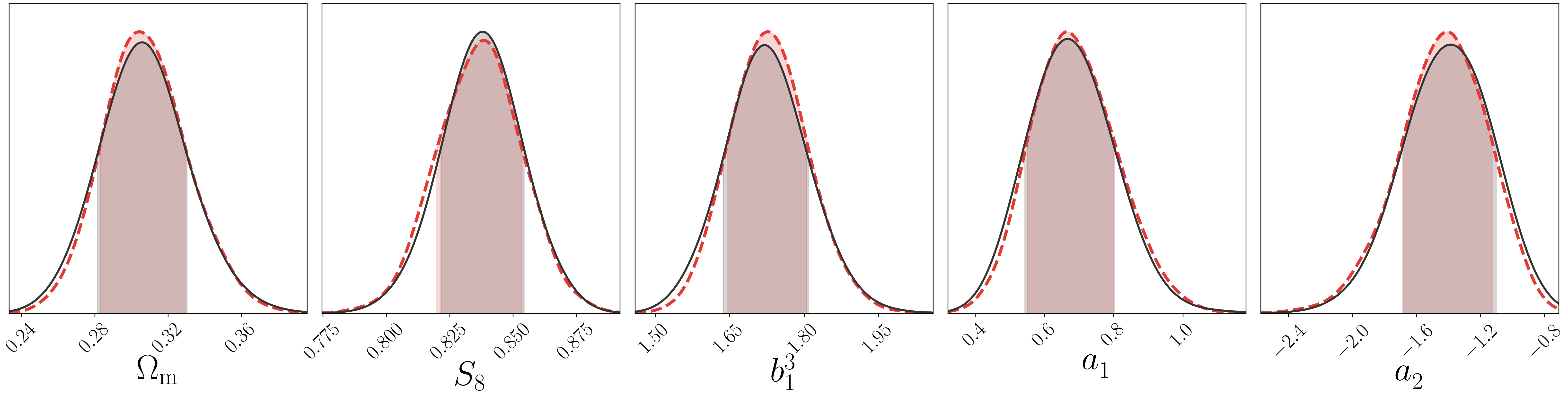
Figure 1: 1D-marginalized parameter posteriors for select parameters obtained for baseline 3$\times$2pt-redMaGiC analyses with CosmoLike analyzing an input data vector generated by CosmoSIS (black solid) and CosmoSIS analyzing an input data vector generated by CosmoLike (red dashed). The agreement of the mean posterior values demonstrates that the $\Delta\chi^{2}<0.2$ difference between model data vectors obtained from the two codes (at the fiducial parameter parameter point) is negligible.

We have developed two independent implementations of the baseline analysis within CosmoSIS and CosmoLike, which we compare following the procedure from DES Y1 (Krause et al., 2017). These codes use different Boltzmann codes (CAMB or CLASS, respectively) and differ in terms of their structure, interpolation and integration routines. After multiple iterations we achieved an agreement of both pipelines at the level of $\Delta\chi^{2}<0.2$ when comparing two model vectors generated at the fiducial cosmology. A simulated likelihood analysis in the full cosmological and systematics parameter space shows no noticeable differences in the parameter constraints from both codes (c.f. Fig. 1 for an illustration in a subspace of the full parameter space; here $S_{8}=\sigma_{8}\sqrt{\Omega_{\mathrm{m}}/0.3}$ is a derived parameter).

Projection effects on marginalized posteriors

Even in the idealized case of applying the baseline analysis to a synthetic, noiseless data vector generated from the same model, the marginalized parameter posteriors may appear biased from the input parameter values due to parameter volume effects (c.f., Fig. 2) while the maximum a posteriori point (MAP, which is optimized over the full parameter space) recovers the input parameter values. These projection effects can occur when parameters of interest are not fully constrained by the data or are degenerate with other parameters that are prior informed. We note that – within a specific set of model and prior choices – these projection effects decrease as the data’s constraining power increases and are thus not a systematic bias. The size and direction of such projection effects depends on the parameterization and prior choices, the underlying parameter values, as well as the data’s constraining power. This complicates the comparison of marginalized posteriors between different data sets and different analysis choices for the same data (e.g., variations of scale cuts, or model parameterization variations for a specific systematic effect). To indicate possible effects of parameter degeneracies on marginalized parameter constraints, 1D-marginalized DES Y3 results on a parameter $p$ are often reported as

$$p=\text{mean value}^{+{\text{upper 34\%}}}_{-{\text{lower 34\%}}}\;\;\;(\text{MAP value})\,.$$ (36)

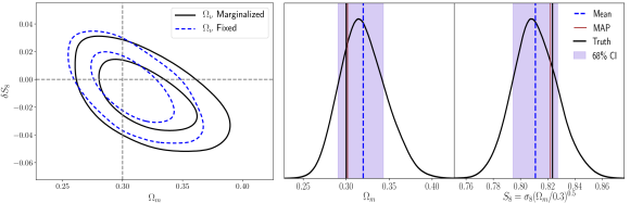
Figure 2: Marginalized 2D and 1D parameter posteriors from simulated 3$\times$2pt $\Lambda$CDM baseline analyses of synthetic, noiseless baseline data vectors.
Left: Marginalized $(\Omega_{\rm m},S_{8})$ posteriors assuming massless neutrinos (blue dashed) and marginalizing over neutrino mass (black solid) using the fiducial value and prior from Table 2. The $S_{8}$ posteriors are shown with respect to its input value in each analysis, which differ due to the difference in input neutrino mass, while the input matter density $\Omega_{\rm m}=\Omega_{\rm{cdm}}+\Omega_{\rm b}+\Omega_{\nu}$ is the same for both analyses (c.f. 2). $\Omega_{\nu}$ is poorly constrained by the 3$\times$2pt analysis and the shift in 2D contours indicates a projection effect from marginalizing over an under-constrained parameter that is correlated with the parameters shown. Center/Right: 1D marginalized posteriors (black curve) in $\Omega_{\rm m}/S_{8}$ for the simulated 3$\times$2pt $\nu\Lambda$CDM baseline analysis (black solid line in the left figure). The vertical black/red lines show the input value and MAP estimate, the blue shaded bands indicate the 1D marginalized, symmetric $68\%$ uncertainty regions. The 1D marginalized mean and posterior distribution are biased from the input parameter value due to projection effect by nearly 1$\sigma$, while MAP closely recovers the input parameters.

IV.2 External Data

The most constraining results on cosmological parameters will be obtained by combining the DES 3$\times$2pt analysis with external data sets, assuming these experiments are sufficiently consistent for a combined analysis. As detailed in Sect. V, we quantify the accuracy of model choices as bias in inferred parameters relative to the expected constraining power, which differ for each analysis (specified by data and parameter spaces). Hence we also need to validate the DES baseline model choices for the more stringent combined analysis. We simulate the constraining power of the external data at our fiducial cosmology, so that parameter biases can be attributed to model choices without any contribution from residual tension between the two experiments. For simulated joint DES-Y3+Planck analyses, we add the constraining power of Planck (TTTEEE+lowE) as a Gaussian prior, computed from the parameter covariance of Planck chains (Planck Collaboration et al., 2020), to our simulated DES-Y3 analyses. This requires approximating the Planck posterior as a Gaussian, which in the parameter dimensions relevant for DES analyses is an acceptable approximation, and shifting the Planck best-fit value to match the fiducial parameter values from Table 2.

V Model Validation

We scrutinize the model choices described in Sect. III.1 closely following the DES-Y1 model validation procedure (Krause et al., 2017), considering two different categories:

• Known, but unmodeled systematic effects, e.g., the impact of baryons on the matter power spectrum, nonlinear galaxy bias. These systematics are mitigated through scale cuts that exclude the affected data points from the analysis.

• Systematics modeled with imperfect parameterizations, which applies to all modeled systematics. We stress test the baseline parameterization to show its robustness.

In practice, we carry out simulated (cosmic shear, 2$\times$2pt, 3$\times$2pt, 3$\times$2pt+Planck) analyses in $\Lambda$CDM and $w$CDM on contaminated data vectors and quantify the 2D parameter bias in $(\Omega_{\mathrm{m}},S_{8})$ for $\Lambda$CDM and in $(\Omega_{\mathrm{m}},w)$ for $w$CDM. We test the impact of different unmodeled systematics in combination by using contaminations at the upper limit of credible severity for each effect. For the second category, we carry out the parameterization stress test for each systematic effect individually using alternative parameterizations as input.

To ensure that the total potential systematic bias is well below $1\sigma$ statistical uncertainty, we require the 2D parameter biases to be smaller than $0.3\sigma_{2\mathrm{D}}$; additionally we require a residual $\Delta\chi^{2}<1$ (after fitting the baseline model to the contaminated data) for each of these tests in order to not bias the goodness of fit. If a model variation changes the data vector by $\Delta\chi^{2}<0.2$ without refitting, we consider this model variation to be insignificant as the change in $\Delta\chi^{2}$ is less than the residual between the two analysis codes. If a model variation changes the data vector by $\Delta\chi^{2}<1$ without refitting, the $\Delta\chi^{2}$ threshold after refitting is automatically met; hence we use importance sampling (IS) of the baseline chain to estimate parameter biases, which is computationally more efficient than carrying out an independent analysis.

We emphasize that all model validation tests in this paper were carried out for both lens samples in parallel, and both lens samples pass these validation criteria. For clarity of presentation, we primarily describe quantitative results for the redMaGiC sample. Corresponding figures and numbers for the maglim sample can be found in Ref. (Porredon et al., 2021).

When small differences in likelihood correspond to a large region in parameter space, e.g., for insufficient or degenerate models, we found MAP parameter estimates to be noisy even with repeated numerical optimization using the Nelder-Mead method (Nelder and Mead, 1965) starting from the best-fit parameter values obtained from likelihood chain. Hence we determine parameter biases from marginalized 2D-parameter posteriors. To account for projection effects, we evaluate parameter biases relative to the marginalized 2D-parameter posteriors of an otherwise identical analysis of the uncontaminated data vector, which is subject to the same projection effects (cf. Fig 4). While the size and direction of parameter projection effects can be altered by large changes in the input parameters, we verified their stability with respect to small fluctuations by analyzing 100 noisy data vector realizations with noise drawn from the data covariance.

V.1 Scale Cuts

For the DES-Y3 baseline model, the largest unmodeled systematics are the impact of baryonic feedback on the matter power spectrum and nonlinear galaxy bias. As both of these effects will affect the 3$\times$2pt data, they need to be mitigated in combination. However, in practice cosmic shear scale cuts are driven by baryonic feedback modifying the matter power spectrum, while nonlinear galaxy biasing is the dominant contamination to galaxy clustering and galaxy-galaxy lensing.

We optimize scale cuts through a series of simulated analyses of a synthetic data vector contaminated by baryonic feedback effects and nonlinear galaxy bias, using different scale cut proposals. If the contamination model assumes a realistic upper boundary for the effect, the analysis will yield unbiased parameter values. The theoretical model error covariance (Baldauf et al., 2016) provides an elegant alternative to scale cuts through analytic marginalization of theoretical model uncertainties. However, this approach requires a model for the distribution of the model error, an assumption that is much more difficult to validate than the choice of one pessimistic contamination realization for scale cuts. It was recently demonstrated (Chudaykin et al., 2020) that the model error covariance for redshift-space galaxy power spectrum analyses can be obtained from large mock catalogs. However, an application to baryonic feedback effects requires additional research, such as how to fairly sample the space of possible feedback models.

V.1.1 Baryon Impact Modeling

We bracket the impact of baryonic physics on the DES data vector using measurements of the matter power spectrum from hydrodynamic simulations with large AGN feedback. As in the DES-Y1 analysis (Krause et al., 2017; Abbott et al., 2018), we use the AGN scenario from the OWLS simulation suite (Schaye et al., 2010; van Daalen et al., 2011), which adopts the AGN subgrid physics under the prescription of Ref. (Booth and Schaye, 2009); black holes inject 1.5% of the rest mass energy of the accreted gas into the surrounding matter in the form of heat.

We consider OWLS-AGN an adequate upper limit for the impact of baryonic physics. Huang et al. (2021) ranked various hydrodynamical scenarios based on the amount of suppression toward small scales against the dark-matter-only theoretical prediction in the cosmic shear statistics (see their Figs. 15 and 16). While more extreme scenarios, most notably the Illustris simulation (Vogelsberger et al., 2014), exist, Illustris is known be too extreme in its radio-mode AGN feedback, and underpredicts the amount of baryons in galaxy groups compared with observations (see Fig.1 of Haider et al. 2016 or Fig.10 of Genel et al. 2014). The successor IllustrisTNG simulation (e.g., see Springel et al., 2018; Pillepich et al., 2018) modifies the original Illustris feedback prescription, resulting in much weaker suppression effect in the summary statistics of power spectrum (see Fig.1 of Ref. (Huang et al., 2021)). The baseline BAHAMAS simulation (McCarthy et al., 2018) is calibrated with observations of the present-day stellar mass function and hot gas fractions in galaxy groups to ensure the overall matter distribution are broadly correct under the effect of baryons. It improves the subgrid models of the OWLS-AGN simulation, which has overly efficient stellar feedback and underpredicts the abundance of $<10^{11}{\rm M}_{\odot}$ galaxies at present day (McCarthy et al., 2017). When performing validation, we thus select the scenario of OWLS-AGN which is more extreme than the BAHAMAS, but below the suppression level of Illustris.

We refer to Huang et al. (2019, 2021) for numerical details on the computation of contaminated DES model data vectors.

V.1.2 Nonlinear Galaxy Bias Modeling

We model the contribution of nonlinear galaxy biasing to galaxy clustering and galaxy-galaxy lensing using an effective 1-loop model with renormalized nonlinear bias parameters (McDonald and Roy, 2009; Baldauf et al., 2012; Chan et al., 2012; Saito et al., 2014), $b_{2}$ (local quadratic bias), $b_{s^{2}}$ (tidal quadratic bias) and $b_{\rm 3nl}$ (third-order nonlocal bias):

$$P_{g\mathrm{m}}(k)= \;b_{1}P_{\mathrm{mm}}(k)+\frac{1}{2}b_{2}P_{b_{1}b_{2}}(k)+\frac{1}{2}b_{s^{2}}P_{\rm b_{1}s^{2}}(k)$$

$$+\frac{1}{2}b_{\rm 3nl}P_{b_{1}b_{\rm 3nl}}(k)\,,$$ (37)

$$P_{gg}(k)= \;b_{1}^{2}P_{\mathrm{mm}}(k)+b_{1}b_{2}P_{\rm b_{1}b_{2}}(k)+b_{1}b_{s^{2}}P_{b_{1}s^{2}}(k)$$

$$+b_{1}b_{\rm 3nl}P_{b_{1}b_{\rm 3nl}}(k)+\frac{1}{4}b_{2}^{2}P_{b_{2}b_{2}}(k)$$

$$+\frac{1}{2}b_{2}b_{s^{2}}P_{b_{2}s^{2}}(k)+\frac{1}{4}b_{s}^{2}P_{s^{2}s^{2}}(k)\,,$$ (38)

where we have omitted the subscript denoting the dependence of bias parameters on the galaxy sample (e.g., $b_{2,g})$ for clarity. Expressions for the power spectrum kernels $P_{b_{1}b_{2}},$ etc., are given in Saito et al. (2014).

This model was found to describe the clustering of redMaGiC-like galaxies in mock catalog at DES-Y3 accuracy down to 4 $\rm{Mpc}/h$ (Pandey et al., 2020). As validated in Pandey et al. (2020), we fix the bias parameters $b_{s^{2}}$ and $b_{\rm 3nl}$ to their co-evolution value of $b_{s^{2}}=-4(b_{1}-1)/7$ and $b_{\rm 3nl}=b_{1}-1$ (Saito et al., 2014). For $b_{2}$, we use values interpolated from the $b_{2}-b_{1}$ relation measured from mock catalogs of redMaGiC-like galaxies (Pandey et al., 2020), $b_{2}(b_{1}=1.7)=0.23,\,b_{2}(b_{1}=2.0)=0.5$. For comparison, $b_{2,\rm{halo}}(b_{1,\rm{halo}}=1.7)=-0.51,\,b_{2,\rm{halo}}(b_{1,\rm{halo}}=2.0)=-0.09$ using the fitting function of Lazeyras et al. (2016) for halos. To motivate our choice for $b_{2}$, we calculate the impact of broad halo occupation distributions (HOD) by averaging $b_{2,\rm{halo}}(b_{1,\rm{halo}})$ over HODs that are only constrained by the redMaGiC abundance and linear bias values (c.f. discussion of galaxy bias in Sect. V for details on these HODs). Figure 3 shows that the $b_{2}$ values measured in mocks are consistent with those expected for galaxy samples with a broad halo mass distribution.

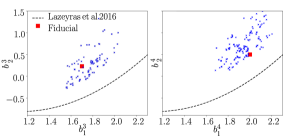
Figure 3: Relation between linear bias $b_{1}$ and local quadratic bias $b_{2}$ for halos (Lazeyras et al., 2016, dashed line) and galaxies (blue crosses), obtained by averaging the halo relation over HODs constrained by the redMaGiC abundance and linear bias values (blue crosses), for tomographic lens bins 3 (left) and 4 (right). The red squares denote the values used to compute the nonlinear bias contamination in Sect. V.1.

V.1.3 Scale Cut Analyses

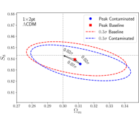
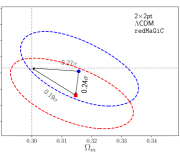
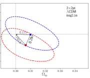
Figure 4: Parameter biases for final scale cuts in $\Lambda\mathrm{CDM}$: the red and blue ellipses show $0.3\,\sigma$ contours for the 2D marginalized constraints of the baseline and contaminated data vector, respectively. Due to parameter volume effects, the marginalized constraints from the baseline analysis are not centered on the input cosmology, and the parameter bias due to unaccounted systematics is given by the offset between the red and blue contours. Left: Simulated cosmic shear analyses. Center: Simulated 2$\times$2pt-redMaGiC analyses. Right: Simulated 2$\times$2pt-maglim analyses. The dashed horizontal and vertical lines indicate the input parameter values.

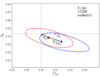
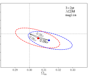
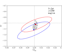
Figure 5: Same as Fig. 4 for 3$\times$2pt-analyses in $\Lambda\mathrm{CDM}$ and $w\mathrm{CDM}$ analyses. Left: Simulated $\Lambda\mathrm{CDM}$ 3$\times$2pt-redMaGiC analyses. Center: Simulated $\Lambda\mathrm{CDM}$ 3$\times$2pt-maglim analyses. Right: Simulated $w\mathrm{CDM}$ 3$\times$2pt-maglim analyses.

We generate data vectors with the baryonic feedback and nonlinear bias contamination models described above, and run simulated likelihood analyses for a family of angular scale cut proposals: for galaxy clustering and galaxy-galaxy lensing, we vary the minimum comoving transverse scale $R_{\rm{min}}$ included in the analysis, corresponding to an angular scale cut $\theta_{\mathrm{min}}^{i}=R_{\mathrm{min},w/\gamma_{\rm{t}}}/\chi(z^{i})$ for each tomographic lens bin $i$.

For cosmic shear, we choose a threshold $\Delta\chi^{2}_{\rm{thr}}$ value for the difference between contaminated and baseline cosmic shear data vectors, and then determine scale cuts $\theta_{\rm{min},\pm}^{ij}$ for each pair of source bins such that the baryonic contamination results in $\Delta\chi^{2}(\xi_{\pm}^{ij})<\Delta\chi^{2}_{\rm{thr}}/20$ for each of the 20 shear 2pt functions (10 different tomographic combinations each for $\xi_{+}$ and $\xi_{-}$).

While scale cuts need to be tested for each analysis setup (choice of probes, model space, and parameters of interest), we require the same scale cuts for cosmic shear, 2$\times$2pt, 3$\times$2pt and 3$\times$2pt+Planck in $\Lambda$CDM and $w$CDM analyses in order to enable model comparisons based on the same data points. We find that scale cuts corresponding to the parameters

$$\left(R_{\mathrm{min},w},\,R_{\mathrm{min},\gamma_{\rm{t}}},\Delta\chi^{2}_{\rm{thr}}\right)=\big{(}8\,\mathrm{Mpc}/h,\,6\,\mathrm{Mpc}/h,\,0.5\big{)}\,$$ (39)

meet our parameter bias requirements for all these analyses. Figure 4 illustrates the residual $\Lambda$CDM parameter biases in cosmic shear, 2$\times$2pt and 3$\times$2pt. The corresponding 2D parameter bias for 3$\times$2pt+Planck ($\Lambda$CDM) is $0.02\sigma_{\mathrm{2D}}$; for $w$CDM we found parameter biases of $0.1\sigma_{\mathrm{2D}}$, $0.16\sigma_{\mathrm{2D}}$ and $0.05\sigma_{\mathrm{2D}}$ for 2$\times$2pt, 3$\times$2pt, and 3$\times$2pt+Planck respectively.

At these fiducial scale cuts, even an extreme contamination such as the Illustris feedback model only results in a $0.23\sigma_{\mathrm{2D}}$ and $0.50\sigma_{\mathrm{2D}}$ for shear and 3$\times$2pt ($\Lambda$CDM), respectively, which demonstrates the robustness of our analysis choices.

In addition to the fiducial scale cuts described above, Amon et al. (2021); Secco et al. (2021) introduce scale cuts for an “optimized” cosmic shear analysis, which maximizes the constraining power of cosmic shear, such that $\sigma_{2\mathrm{D},3\times 2\text{pt}}=0.3$ in $\Lambda$CDM. For the cosmic shear analysis, these optimized scale cuts result in $\sigma_{2\mathrm{D},\text{1x2pt}}=0.1$. The corresponding scale cuts were obtained by iteratively removing the data point from the tomographic cosmic shear data vector with the largest contribution to $\Delta\chi^{2}$, until the baryonic contamination results in a residual $\Delta\chi^{2}=1$. $\Lambda$CDM constraints from a 3$\times$2pt analysis based on these optimized cosmic shear scale cuts are presented in Ref. (DES Collaboration, 2021). We note that this scale cut choice does not pass the validation criteria in $w$CDM and that it was introduced after unblinding of the cosmology results.

V.2 Model Parameterization Stress Tests

V.2.1 Matter Power Spectrum

In order to bracket potential parameter biases due to the accuracy limitations of halofit for the nonlinear gravity-only power spectrum, we compare to the Cosmic Emu (Lawrence et al., 2017) and Euclid Emulator (Euclid Collaboration et al., 2019) emulators, which are based on larger, more recent simulations and thus provide higher model accuracy. These more accurate emulators are designed for a limited range in cosmological parameter space, which does not cover the expected $2\sigma$ parameter uncertainty regions of DES-Y3 cosmic shear and 2$\times$2pt analyses. Hence current emulators are well suited for validation at selected cosmologies, but are not a practicable alternative for the baseline model.

For completeness, we also compare to the HMCode fitting function (Mead et al., 2015). Figure 6 shows the result of analyzing simulated data vectors computed from these alternate prescriptions for the nonlinear gravity-only power spectrum with halofit. We find insignificant parameter biases relative to the two emulator models ($<0.15\sigma_{2\rm{D}}$). We note that the comparison of HMCode and halofit fails our requirements for the 2$\times$2pt analysis. The Mead et al. (2015) version of HMCode employed here is known to overpredict the power spectrum in the quasilinear regime ($k\sim 0.1\dots 0.5h/\mathrm{Mpc}$, (c.f. Fig. 1 of Joachimi et al., 2021)); the DES 2$\times$2pt analysis is particularly sensitive to these scale due to the clustering scale cut $R_{\mathrm{min},w}=8\mathrm{Mpc/h}$. While these comparisons indicate that halofit is sufficient for the DES-Y3 baseline analysis, the accuracy requirements of future weak lensing surveys on matter power spectrum modeling (e.g., Martinelli et al., 2021) may require a new generation of models/emulators with sufficient support in parameters.

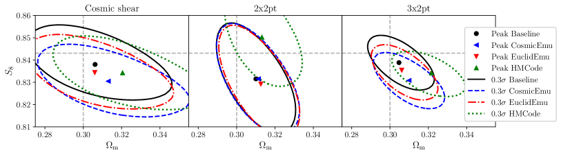
Figure 6: Robustness of parameter constraints to the choice of matter power spectrum model. The black contour shows the $0.3\sigma_{2\rm{D}}$ baseline analysis results (analyzing halofit input with halofit model). The blue/red/green contours illustrate the systematic bias, estimated through importance sampling, when input data from Cosmic Emu/Euclid Emulator/HMCode is analyzed with halofit. All contours levels are $0.3\sigma_{2\rm{D}}$, and symbols indicate the 2D (marginalized) peak.

V.2.2 Galaxy Bias

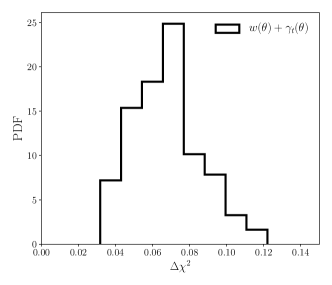
Figure 7: Impact of galaxy bias redshift evolution on DES 2pt statistics: We compute $\Delta\chi^{2}$ between models with galaxy bias constant within each tomographic bins, and models with evolving galaxy bias based on the redshift evolution of the halo mass function and halo mass–bias relation, assuming a constant HOD within each tomographic bin. The histogram shows the $\Delta\chi^{2}$ distribution when sampling HOD parameters that are constrained only by the fiducial linear bias value and observed galaxy number density.

The scale cuts derived in Sect. V.1 are designed to enable a linear galaxy bias baseline model. It remains, then, to validate the assumption that these linear bias parameters can be modeled as constant within each tomographic bin. Two independent mock catalogs (DeRose et al., 2019; Carretero et al., 2015) display limited redshift evolution of the HOD of redMaGiC galaxies within the relatively narrow ($\Delta z=0.15$) tomographic bins. Hence we model the potential redshift evolution of galaxy bias within tomographic bins based on the redshift evolution of the halo mass function and halo mass–halo bias relation assuming a constant HOD. For each tomographic bin, we generate samples of possible HODs using the parameterization from Ref. (Zheng et al., 2005) for luminosity threshold samples, with an additional parameter to account for the incompleteness of central galaxies in a color-selected sample, constrained by the fiducial linear bias values and observed number density (see Pandey et al., 2021, for details). Figure 7 shows that this model for bias redshift evolution results in $\Delta\chi^{2}<0.2$. Hence we expect the redshift evolution of galaxy bias to have negligible impact on parameter constraints, even if one allowed for redshift evolution of the HOD within $\Delta z=0.15$ tomographic bins.

We also tested that the scale dependence of galaxy bias imparted by massive neutrinos (LoVerde, 2014) has no significant impact on inferred parameters.

V.2.3 Intrinsic Alignments

The TATT model adopted as the baseline intrinsic alignment parameterization includes two next-to-leading order effects (density weighting, tidal torquing) which are theoretically well-motivated but observationally less well studied. Samuroff et al. (2019) found an indication for nonzero values of the associated parameters ($b_{\mathrm{ta}},a_{2}$) at around the $1\sigma$ level in cosmic shear alone, with the less constraining DES-Y1 data. We thus include these parameters in the fiducial setup, which was frozen before unblinding of the DES-Y3 analysis, noting that their redshift evolution has not yet been constrained. Also before unblinding, it was agreed to characterize their redshift evolution in post-unblinding work (Secco et al., 2021) if the DES-Y3 analysis found these types of intrinsic alignment effects to be significant.

While perturbative IA models that are more complete and extend to higher order than TATT exist (Vlah et al., 2020), there are no observational constraints on the additional parameters. Due to the lack of realistic amplitudes for higher-order IA contaminations, we do not use a strategy analogous to the perturbative bias contamination in Sect. V.1 to test whether TATT is sufficient to model the scale-dependence of IA in the context of this analysis. Furthermore, we do not test robustness to fully nonlinear IA contributions, noting that (Fortuna et al., 2020) found the 1-halo IA contamination unlikely to significantly bias current generation lensing studies.

The redshift and galaxy luminosity dependence of NLA have been characterized (for elliptical galaxies) over limited ranges in luminosity and redshift (Joachimi et al., 2011; Singh et al., 2015). Assuming that only red galaxies are subject to linear alignments, one can predict the mean NLA amplitude of the DES source sample as a function of redshift through extrapolation (in luminosity and redshift) of the observed NLA scalings down to the limiting magnitude over the redshift range (Krause et al., 2016). This estimate further requires extrapolation of an observed luminosity function for all and red galaxies in order to model the red fraction of galaxies (Krause et al., 2016). The redshift evolution predicted from extrapolation of the NLA amplitude of the MegaZ-Luminous Red Galaxy sample and the DEEP2 luminosity functions (Faber et al., 2007) is not monotonic and not well described by a power law. This prescription was used in DES Y1 (Krause et al., 2017) to demonstrate that a power law parameterization for the NLA redshift evolution was sufficient for the DES-Y1 analysis, and predicted an NLA amplitude for the DES-Y1 source sample $A_{1}(z_{0})$ consistent with the constraints obtained in Ref. (Abbott et al., 2018).

For DES-Y3, this model for the redshift dependence of $A_{1}$ results in parameter shifts up to $0.5\sigma_{2\rm{D}}$ for cosmic shear alone in the context of the TATT model with fiducial $a_{2},\,\eta_{2},\,b_{\mathrm{ta}}$ value. It does not result in significant biases for 2$\times$2pt or 3$\times$2pt analyses and passes our requirements, except for the cosmic shear analysis. Hence we validate the robustness of this parameterization a posteriori on data. This a posteriori validation procedure, as well as several additional IA model robustness tests for cosmic shear analyses, are presented in Secco, Samuroff et al. (2021). We note that the realism of this model stress test is questionable as it is based on several extrapolations ($z-$ and $L-$ scaling of observed $A_{1}$; $z$, $L$ dependence of the luminosity function for all and red galaxies). Due to the absence of a sharp test or other well-motivated parameterizations, we proceed with the baseline power-law redshift evolution parameterization and a posteriori validation on data.

V.2.4 Magnification

Elvin-Poole et al. (2021) demonstrate that DES-Y3 cosmology constraints are robust to biases in the estimated values for $C_{\rm{l}}^{i}$, including the extreme scenario of $C_{\rm{l}}^{i}=0$, i.e., ignoring lens magnification in the analysis. Hence we leave tests of the redshift evolution of these coefficients to future analyses, for which lens magnification is forecasted to become a significant systematic (Lorenz et al., 2018; Thiele et al., 2020).

V.2.5 Higher-Order Lensing Effects

The calculations of angular statistics described in Sect. II included only leading-order lensing effects. The most significant next-to-leading-order contributions to the observed two-point statistics are reduced shear (Dodelson et al., 2006; Shapiro, 2009) and source clustering and magnification (Schneider et al., 2002a; Schmidt et al., 2009b), while distortions from multiple deflections can safely be ignored (Cooray and Hu, 2002; Krause and Hirata, 2010). We review these effects below, and derive expressions for the impact of source clustering applicable to broad tomographic source bins.

Each of these effects amounts to weighting the shear by another field (convergence, galaxy density, deflection angle, respectively), and this mode coupling gives rise to small amounts of shear B-modes. As the resulting B-mode power spectra are negligible even for the next generation of weak lensing surveys, we focus here on the (larger) leading E-mode corrections.

Reduced Shear

As the intrinsic size of source galaxies is unknown, galaxy-shape distortions measure the reduced shear, $g=\gamma/(1+\kappa)$ rather than $\gamma$. The leading correction is

$$g_{\alpha,\mathrm{obs}}^{i}(\hat{\mathbf{n}})=\frac{\gamma_{\alpha,\mathrm{obs}}^{i}(\hat{\mathbf{n}})}{1-\kappa^{i}(\hat{\mathbf{n}})}\approx\gamma_{\alpha,\mathrm{obs}}(\hat{\mathbf{n}})+\gamma_{\alpha,\mathrm{obs}}(\hat{\mathbf{n}})\kappa^{i}(\hat{\mathbf{n}})\,.$$ (40)

The corresponding correction to the E-mode power spectrum is (Dodelson et al., 2006; Shapiro, 2009)

$$\Delta C_{{EE}}^{ij}(\ell)= \int\frac{d\chi}{\chi^{4}}\,W^{i}_{\kappa,\mathrm{s}}(\chi)W^{j}_{\kappa,\mathrm{s}}(\chi)\left[W^{i}_{\kappa,\mathrm{s}}(\chi)+W^{j}_{\kappa,\mathrm{s}}(\chi)\right]$$

$$\times\int\frac{d^{2}L}{(2\pi)^{2}}\cos(2\phi_{L})B_{\mathrm{m}}\left(\frac{\mathbf{L}}{\chi},\frac{\bm{\ell}-\mathbf{L}}{\chi},\frac{-\bm{\ell}}{\chi},\chi\right)$$

$$+\int\frac{d^{2}L}{(2\pi)^{2}}\cos(2\phi_{L})\left[\cos(2\phi_{L})+\cos(2\phi_{\mathbf{L}-\bm{\ell}})\right]$$

$$\quad\times\,C_{\kappa\kappa}^{ij}(L)\,C_{\kappa\kappa}^{ij}(|\mathbf{L}-\bm{\ell}|)$$

$$+\left[C_{\kappa\kappa}^{ii}(\ell)\int\frac{dL}{2\pi}L\,C_{\kappa\kappa}^{jj}(L)+\left(i\leftrightarrow j\right)\right]\,,$$ (41)

with $B_{\mathrm{m}}(\mathbf{k_{1}},\mathbf{k_{2}},\mathbf{k_{3}},\chi)$ the matter bispectrum at redshift $z(\chi)$, and where we have omitted the reduced shear effect on $\gamma_{\mathrm{IA}}$. While the three terms in Eq. (41) are of the same order in the linear matter density contrast, the last two terms containing products of two angular convergence power spectra are strongly suppressed as they include an additional lens efficiency factor. The B-mode power spectrum from reduced shear is given by convolution of two angular convergence power spectra with different phase factor (there is no bispectrum term as the first-order B-mode shear is zero); as it is known to be insignificant (Schmidt et al., 2009b; Krause and Hirata, 2010), we will not consider it further here. For galaxy-galaxy lensing,

$$\Delta C^{ij}_{\delta_{\mathrm{l}}E}(\ell)= \int\frac{d\chi}{\chi^{4}}\left[b^{i}_{1,\mathrm{l}}W^{i}_{\delta,\mathrm{l}}(\chi)+C^{i}_{\mathrm{l}}W^{i}_{\kappa,\mathrm{l}}(\chi)\right]\left(W^{j}_{\kappa,\mathrm{s}}(\chi)\right)^{2}$$

$$\times\int\frac{d^{2}L}{(2\pi)^{2}}\cos(2\phi_{L})B_{\mathrm{m}}\left(\frac{\mathbf{L}}{\chi},\frac{\bm{\ell}-\mathbf{L}}{\chi},\frac{-\bm{\ell}}{\chi},\chi\right)\,.$$ (42)

Source Clustering and Magnification

Since the shear field is only observed at the positions of source galaxies, we now account for deviations from the mean source redshift distribution along specific lines of sight due to the physical (3D) clustering of sources and modulation of the selection function by magnification:

$$n_{\mathrm{s}}^{i}(\chi)\rightarrow n_{\mathrm{s}}^{i}(\chi)\left[1+{\delta^{(3\mathrm{D})}_{\mathrm{s}}(\hat{\mathbf{n}}\chi,\chi)}{\color[rgb]{0,0,0}}\right]\left[1+C_{\mathrm{s}}^{i}\kappa\left(\hat{\mathbf{n}},z\right)\right]\,.$$ (43)

Here we have introduced the convergence field of a source plane at redshift $z$

$$\kappa\left(\hat{\mathbf{n}},z\right) =\frac{3\Omega_{\mathrm{m}}H_{0}^{2}}{2c^{2}}\int_{0}^{z(\chi)}d\chi\,\frac{\chi}{a(\chi)}\frac{\chi(z)-\chi}{\chi(z)}\delta_{\mathrm{m}}(\hat{\mathbf{n}}\chi,\chi)$$

$$=\int_{0}^{\chi(z)}d\chi\,W_{\kappa}(\chi,z)\,\delta_{\mathrm{m}}(\hat{\mathbf{n}}\chi,\chi)\,,$$ (44)

where in the second step we defined $W_{\kappa}(\chi,z)$, the lens efficiency of a source plane at redshift $z$.

The corresponding corrections to the shear field are computed starting from the deflection tensor (Eq. 8) with the modified redshift distribution,

$$\Delta\Psi_{\alpha\beta}(\bm{\ell}) = 2\int\!\!\frac{d^{2}L}{(2\pi)^{2}}\int\!d\chi\;n_{\mathrm{s}}^{i}(\chi)\Bigg{[}b_{1,\mathrm{s}}^{i}\delta_{\mathrm{m}}((\bm{\ell}-\mathbf{L})/\chi,\chi)$$ (45)

$$+C_{\mathrm{s}}^{i}\int_{0}^{\chi}\!\!\!d\chi^{\prime\prime}W_{\kappa}(\chi^{\prime\prime},z(\chi))\delta_{\mathrm{m}}((\bm{\ell}-\mathbf{L})/\chi^{\prime\prime},\chi^{\prime\prime})\Bigg{]}$$

$$\times\int_{0}^{\chi}\!\!\!d\chi^{\prime}W_{\kappa}(\chi^{\prime},z(\chi))\frac{L_{\alpha}L_{\beta}}{L^{2}}\delta_{\mathrm{m}}\left(\mathbf{L}/\chi^{\prime},\chi^{\prime}\right),$$

where we omitted the $\mathcal{O}\left(\delta_{\mathrm{m}}^{3}\right)$ term as the corresponding $\mathcal{O}\left(\delta_{\mathrm{m}}^{4}\right)$ power spectrum correction vanishes after carrying out the $\phi_{L}$ integral. Projection into shear components (Eqs. 7+11) yields

$$\Delta\gamma_{E}^{i}(\bm{\ell}) = \!\!\int\!\!\frac{d^{2}L}{(2\pi)^{2}}\int\!d\chi\;{n}_{\mathrm{s}}^{i}(\chi)\Bigg{[}b_{1,\mathrm{s}}^{i}\delta_{\mathrm{m}}((\bm{\ell}-\mathbf{L})/\chi,\chi)$$

$$+C_{\mathrm{s}}^{i}\int_{0}^{\chi}\!\!\!d\chi^{\prime\prime}W_{\kappa}(\chi^{\prime\prime},z(\chi))\delta_{\mathrm{m}}((\bm{\ell}-\mathbf{L})/\chi^{\prime\prime},\chi^{\prime\prime})\Bigg{]}$$

$$\times\underbrace{T_{\alpha}(\bm{\ell})T_{\alpha}(\mathbf{L})}_{\cos(2\phi_{L})}\int_{0}^{\chi}\!\!\!d\chi^{\prime}W_{\kappa}(\chi^{\prime},z(\chi))\delta_{\mathrm{m}}\left(\mathbf{L}/\chi^{\prime},\chi^{\prime}\right).$$

The correction $\Delta\gamma_{B}$ is of the same form as Eq. LABEL:eq:g_E, with $T_{\alpha}(\mathbf{l})T_{\alpha}(\mathbf{L})\rightarrow\epsilon_{\alpha\beta}T_{\alpha}(\mathbf{l})T_{\beta}(\mathbf{L})=\sin(2\phi_{L})$.

The resulting power spectrum corrections are then straightforward to calculate. While the source clustering fluctuations in Eq. 43 are orders of magnitudes larger than the magnification fluctuations, several of the corresponding power spectrum correction terms are suppressed by the lens efficiency being zero at the source plane ($W_{\kappa}(\chi(z),z)=0$). There are three different (22)-type corrections to $C_{{EE/BB}}$ permitted under the Limber approximation. As for reduced shear, these terms are much smaller than the bispectrum terms, and we show here only the dominant term, proportional to the source clustering power spectrum,

$$\Delta C^{ij}_{{EE}}(\ell)= \;C_{\mathrm{s}}^{i}\int d\chi\,n_{\mathrm{s}}^{i}(\chi)\int_{0}^{\chi}\!\frac{d\chi^{\prime}}{\chi^{\prime 4}}W_{\kappa,\mathrm{s}}^{j}(\chi^{\prime})W^{2}_{\kappa}\left(\chi^{\prime},z(\chi)\right)\int\!\frac{d^{2}L}{(2\pi)^{2}}\cos(2\phi_{L})B_{\mathrm{m}}\!\left(\frac{\mathbf{L}}{\chi^{\prime}},\frac{\bm{\ell}-\mathbf{L}}{\chi^{\prime}},\frac{-\bm{\ell}}{\chi^{\prime}},\chi^{\prime}\right)+\left(i\leftrightarrow j\right)$$

$$+\int d\chi\!\frac{b_{1,\mathrm{s}}^{i}b_{1,\mathrm{s}}^{j}n_{\mathrm{s}}^{i}(\chi)n_{\mathrm{s}}^{j}(\chi)}{\chi^{2}}\int\!\frac{d^{2}L}{(2\pi)^{2}}\cos^{2}(2\phi_{L})P_{\mathrm{m}}\left(\frac{|\bm{\ell}-\mathbf{L}|}{\chi},\chi\right)\int_{0}^{\chi}d\chi^{\prime}\frac{W^{2}_{\kappa}\left(\chi^{\prime},z(\chi)\right)}{\chi^{\prime 2}}P_{\mathrm{m}}\left(\frac{L}{\chi^{\prime}},\chi^{\prime}\right)+\cdots$$ (47)

$$\Delta C^{ij}_{{BB}}(\ell)= \int\!d\chi\frac{b_{1,\mathrm{s}}^{i}b_{1,\mathrm{s}}^{j}n_{\mathrm{s}}^{i}(\chi)n_{\mathrm{s}}^{j}(\chi)}{\chi^{2}}\int\!\frac{d^{2}L}{(2\pi)^{2}}\sin^{2}(2\phi_{L})P_{\mathrm{m}}\left(\frac{|\bm{\ell}-\mathbf{L}|}{\chi},\chi\right)\int_{0}^{\chi}\!d\chi^{\prime}\frac{W^{2}_{\kappa}\left(\chi^{\prime},z(\chi)\right)}{\chi^{\prime 2}}P_{\mathrm{m}}\left(\frac{L}{\chi^{\prime}},\chi^{\prime}\right)+\cdots$$ (48)

$$\Delta C^{ij}_{\delta_{\mathrm{l}}E}(\ell)= C_{\mathrm{s}}^{j}\int\!d\chi\,n_{\mathrm{s}}^{j}(\chi)\int_{0}^{\chi}\!\frac{d\chi^{\prime}}{\chi^{\prime 4}}\left[b^{i}_{1,\mathrm{l}}W^{i}_{\delta,\mathrm{l}}(\chi^{\prime})+C^{i}_{\mathrm{l}}W^{i}_{\kappa,\mathrm{l}}(\chi^{\prime})\right]W^{2}_{\kappa}\left(\chi^{\prime},z(\chi)\right)\int\!\frac{d^{2}L}{(2\pi)^{2}}\cos(2\phi_{L})B_{\mathrm{m}}\!\left(\frac{\mathbf{L}}{\chi^{\prime}},\frac{\mathbf{l}-\mathbf{L}}{\chi^{\prime}},\frac{-\mathbf{l}}{\chi^{\prime}},\chi^{\prime}\right).$$ (49)

One can read off two useful observations about source clustering from these expressions: first, under the Limber approximation there notably are no bispectrum-type corrections from physical source (or lens-source) clustering, which would originate from the $\delta_{\mathrm{s}}^{(3\mathrm{D})}$ term in Eq. 43, but are suppressed by the source plane lens efficiency. This is in contrast to the projected source clustering ansatz $\gamma^{i}(\hat{\mathbf{n}})\rightarrow\gamma^{i}(\hat{\mathbf{n}})\left(1+\delta^{i}_{\mathrm{s,obs}}(\hat{\mathbf{n}}\right)$ (Schmidt et al., 2009b). For broad tomographic source redshift bins, as applicable to DES-Y3, their approach gives rise to a spurious $\gamma^{i}\delta^{i}_{\mathrm{s,D}}$ term, which would cause substantial parameter biases for the DES-Y3 analysis. In the limit of narrow tomographic bins (considered by Schmidt et al., 2009b), both approaches yield the same power spectrum corrections. Second, $\mathcal{O}\left(\delta_{\mathrm{m}}^{4}\right)$ lens-source clustering corrections to the galaxy-galaxy lensing power spectrum (Eq. 49) vanish under the Limber approximation, which is relevant to the discussion of correlation function estimator effects.

The DES-Y3 analysis adopts pair-based estimators (Landy and Szalay, 1993; Schneider et al., 2002b; Sheldon et al., 2004) for the 2PCF measurements, with weighting schemes (Rodríguez-Monroy et al., 2021; Prat et al., 2021; Amon et al., 2021) (for clustering, galaxy-galaxy lensing, and cosmic shear, respectively). These estimators normalize the galaxy-galaxy lensing/cosmic shear 2PCF measurements by the observed (weighted) lens-source/source-source pair counts in each angular bin, which introduces a modulation by the projected lens-source/source-source clustering correlation functions. For galaxy-galaxy lensing, this modulation describes the dilution by excess (clustered) lens-source pairs at the lens redshift; the DES Y3 galaxy–galaxy lensing analysis (Prat et al., 2021) corrects for it at the measurement level through so-called Boost factors $B^{ij}(\theta)\approx 1+w_{\rm{ls}}^{ij}(\theta)$ (Hirata et al., 2004; Mandelbaum et al., 2005). This effect is separate from the source clustering effect derived here, as is evident from the absence of $\mathcal{O}\left(\delta_{\mathrm{m}}^{4}\right)$ terms in Eq. (49).

The measured cosmic shear correlation functions $\xi_{\pm}$ are not debiased for the modulation of the observed pair counts by $(1+w_{\rm{ss}}^{ij}(\theta))$ from the pair-based estimator (Schneider et al., 2002a; Schmidt et al., 2009b). This effect is partially cancelled by the (22)-type corrections to $C_{{EE/BB}}$ shown in Eqs. (47,48): for $\xi+$, in the limit of narrow source redshift bins (and hence restricting to auto-tomography combinations, $i=j$), the sum of these two corrections simplifies to the convolution of the convergence and angular source clustering power spectra

$$\Delta C^{(\mathcal{O}(\delta_{\mathrm{m}}^{4}))}_{{EE}}(\ell)+\Delta C_{{BB}}(\ell)\approx\left[C_{\kappa\kappa}*C_{\delta_{\rm{s}}\delta_{\rm{s}}}\right](\ell)\,,$$ (50)

corresponding to $\Delta\xi_{+}(\theta)=\xi_{+}(\theta)w_{\mathrm{ss}}(\theta)$ in configuration space .

We evaluate the combined effect of reduced shear and source clustering assuming $b^{i}_{1,\mathrm{s}}=1$ and source magnification coefficients $C_{\mathrm{s}}^{1\cdots 4}=\left(-1.17,-0.64,-0.55,0.80\right)$, estimated from data (Elvin-Poole et al., 2021), and modeling the matter bispectrum as tree-level but replacing the linear matter power with the nonlinear matter power spectrum (see Lazanu et al., 2016, for a detailed analysis of bispectum models). The combined impact of higher-order lensing effects on parameter estimates is shown in Fig. 8 for DES-Y3 $\Lambda$CDM analyses; the two-dimensional parameter bias is below $0.15\sigma_{2\mathrm{D}}$ for all analyses.

We note that impact of reduced shear and source clustering on cosmic shear and galaxy-galaxy lensing is sensitive to squeezed-limit bispectrum configurations and thus the nonlinear bispectrum model. Accurate modeling of these effects will be required for weak lensing analyses of future surveys.

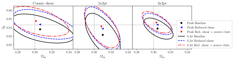
Figure 8: Robustness of parameter constraints to higher-order lensing effects. The offset between the blue/red contour and black contour illustrates the systematic bias incurred by neglecting reduced shear/reduced shear and source clustering terms. The contours levels are $0.3\sigma_{2\rm{D}}$, symbols indicate the 2D (marginalized) peak.

VI Summary and Conclusions

In order to obtain the best possible cosmological parameter constraints, the accuracy of analysis methodology has to be matched to the precision enabled by the data set. Hence the required accuracy depends on the survey properties, the combination of cosmological probes, and the model/parameter space under investigation. The analysis choices that must be made as part of the methodology development range from modeling that is critical to capturing the underlying physics, such as intrinsic alignments, to extensive validation of scale cuts imposed on the data vector, to technical decisions such as prior ranges or the precision of integration and interpolation routines that are employed in the modeling. The limiting factor in some cases is computing time; while of course the pipeline must be sufficiently accurate to match the precision of the data, it is also clear that increasing the complexity of the pipeline at a disproportionately high cost in computing time is unwise if the improvements are well below the statistical errors.

In this paper we describe the cosmology and astrophysics modeling strategy and validation for the DES Y3 joint weak lensing and galaxy clustering analysis. We demonstrate that our analysis choices are sufficient to mitigate systematic biases in the DES Y3 parameter constraints due to theoretical modeling simplifications and uncertainties.

Our modeling systematics mitigation strategy can be summarized as a combination of (1) modeling and marginalizing over systematic-error parameterizations and (2) imposing scale cuts that exclude data points where unmodeled systematics are prevalent. In terms of modeling and marginalizing, we choose a baseline analysis parameterization that models the nonlinear matter power spectrum, galaxy bias, intrinsic alignments, lens magnification, and non-local contributions to galaxy–galaxy lensing. While necessarily incomplete, this model is sufficiently complex and robust for the DES Y3 3$\times$2pt analysis. Specifically, we demonstrate through a large number of simulated likelihood analyses that (1) angular scale cuts mitigate the leading known, but unmodeled, systematic effects, and (2) the baseline parameterization is sufficiently flexible to marginalize over plausible variations from these parameterization choices. We further validate our numerical implementation by comparing independently-developed modeling pipelines, and find them to be in excellent mutual agreement. We conclude that the cosmology and astrophysics modeling is robust within the analysis choices derived here, and that theoretical modeling systematics are insignificant for DES Y3 cosmic shear, 2$\times$2pt and 3$\times$2pt analyses, as well as their combinations with external data. To our knowledge, this work presents the most detailed validation of a large-scale structure survey to date.

The dominant systematics limiting the constraining power of the DES Y3 baseline analyses are astrophysical effects in the nonlinear regime, in particular nonlinear galaxy bias, baryonic effects on the matter power spectrum, and non-local contributions from the one-halo and one-to-two halo transition regime to the large-scale galaxy–galaxy lensing signal. The former two set the angular scale cuts for the baseline analysis, excluding a substantial fraction of the measured signal-to-noise in the two-point correlation functions, while the latter degrades the constraining power of small-scale galaxy–galaxy lensing.

The modeling challenges described in this paper have long been recognized. Successfully resolving them will allow us to achieve the ultimate goal of optimally extracting information from galaxy surveys, particularly from small spatial scales where a large but challenging-to-model signal resides. While our work here represents important developments in mitigating these uncertainties, substantial progress remains possible with future effort. For instance, suitable modeling or mitigating of baryonic effects on small scales can be used to extract more information from weak lensing surveys, as demonstrated by Asgari et al. (2020) and Huang et al. (2021) with recent data sets. Another example is nonlinear galaxy bias: while its modeling has become a standard tool in analyses of galaxy clustering in redshift space (e.g., Sánchez et al., 2017; d’Amico et al., 2020; Ivanov et al., 2020), the application to angular clustering measurements remains challenging due to parameter degeneracies and projection effects. Progress in that particular direction for the DES Y3 analysis is being reported by Pandey et al. (2021) and DeRose et al. (2021), who validate an extension of the baseline analysis described here using next-to-leading-order galaxy biasing; the corresponding gains in constraining power are presented in Ref. (DES Collaboration, 2021). Due to additional nuisance parameters, the gain in constraining power from nonlinear bias modeling is significantly smaller than a mode counting argument might suggest.

Upcoming, more constraining, analyses will continue to balance model accuracy (and hence model complexity) with increased statistical constraining power. One of the main limiting factors for such ambitious analyses will be the availability of sufficient validation tests, such as high-resolution, high-volume mock catalogs that include plausible variations of the relevant nonlinear astrophysics, such as baryonic feedback, or variations in the halo–galaxy connection. This issue will be front-and-center for future analyses of data from Rubin Observatory’s LSST, the Euclid mission, and the Roman Space Telescope, in particular when combining the constraining power of multiple surveys’ data.

Future analyses will need to evaluate the trade-offs that arise from increasing the number of nuisance parameters in the theoretical models. Model complexification can improve the accuracy of cosmological inference by bringing the model space closer to the true Universe. But this may come at the price of increased parameter degeneracies and reduced cosmological precision, inference instabilities due to multiple minima, and biased confidence contours due to prior-volume projections. It is therefore important to develop the least complex analysis that is robust for any given science case and data set, and to attend closely to priors on additional parameters. Mapping out the modeling trade space will require a large set of simulated analyses customized to the noise level, probe combination, and cosmological model space of a given experiment. Advances in theory that restrict rather than expand the model space will be extremely valuable to to achieve high-accuracy cosmology.

References

- Abbott et al. (2018) T. Abbott, F. Abdalla, A. Alarcon, J. Aleksić, S. Allam, S. Allen, A. Amara, J. Annis, J. Asorey, S. Avila, et al., Physical Review D 98 (2018), 10.1103/physrevd.98.043526.
- Hamana et al. (2020) T. Hamana, M. Shirasaki, S. Miyazaki, C. Hikage, M. Oguri, S. More, R. Armstrong, A. Leauthaud, R. Mandelbaum, H. Miyatake, et al., PASJ 72, 16 (2020), arXiv:1906.06041 [astro-ph.CO] .
- Heymans et al. (2021) C. Heymans, T. Tröster, M. Asgari, C. Blake, H. Hildebrandt, B. Joachimi, K. Kuijken, C.-A. Lin, A. G. Sánchez, J. L. van den Busch, et al., A&A 646, A140 (2021), arXiv:2007.15632 [astro-ph.CO] .
- Amon et al. (2021) A. Amon et al., To be submitted to PRD (2021).
- Secco et al. (2021) L. F. Secco, S. Samuroff, et al., To be submitted to PRD (2021).
- Rodríguez-Monroy et al. (2021) M. Rodríguez-Monroy et al., To be submitted to MNRAS (2021).
- Prat et al. (2021) J. Prat et al., To be submitted to PRD (2021).
- Pandey et al. (2021) S. Pandey et al., To be submitted to MNRAS (2021).
- Porredon et al. (2021) A. Porredon et al., To be submitted to PRD (2021).
- DES Collaboration (2021) DES Collaboration, To be submitted to PRD (2021).
- Krause et al. (2017) E. Krause, T. F. Eifler, J. Zuntz, O. Friedrich, M. A. Troxel, S. Dodelson, J. Blazek, L. F. Secco, N. MacCrann, E. Baxter, et al., arXiv e-prints , arXiv:1706.09359 (2017), arXiv:1706.09359 [astro-ph.CO] .
- Joachimi et al. (2021) B. Joachimi, C. A. Lin, M. Asgari, T. Tröster, C. Heymans, H. Hildebrandt, F. Köhlinger, A. G. Sánchez, A. H. Wright, M. Bilicki, et al., A&A 646, A129 (2021), arXiv:2007.01844 [astro-ph.CO] .
- DeRose et al. (2019) J. DeRose, R. H. Wechsler, M. R. Becker, M. T. Busha, E. S. Rykoff, N. MacCrann, B. Erickson, A. E. Evrard, A. Kravtsov, D. Gruen, et al., arXiv e-prints , arXiv:1901.02401 (2019), arXiv:1901.02401 [astro-ph.CO] .
- DeRose et al. (2021) J. DeRose et al., To be submitted to MNRAS (2021).
- Fisher et al. (1994) K. B. Fisher, C. A. Scharf, and O. Lahav, MNRAS 266, 219 (1994), arXiv:astro-ph/9309027 [astro-ph] .
- Padmanabhan et al. (2007) N. Padmanabhan, D. J. Schlegel, U. Seljak, A. Makarov, N. A. Bahcall, M. R. Blanton, J. Brinkmann, D. J. Eisenstein, D. P. Finkbeiner, J. E. Gunn, et al., MNRAS 378, 852 (2007), arXiv:astro-ph/0605302 [astro-ph] .
- Verner Villumsen (1995) J. Verner Villumsen, arXiv e-prints , astro-ph/9512001 (1995), arXiv:astro-ph/9512001 [astro-ph] .
- Moessner and Jain (1998) R. Moessner and B. Jain, MNRAS 294, L18 (1998), arXiv:astro-ph/9709159 [astro-ph] .
- Schmidt et al. (2009a) F. Schmidt, E. Rozo, S. Dodelson, L. Hui, and E. Sheldon, Phys. Rev. Lett. 103, 051301 (2009a), arXiv:0904.4702 [astro-ph.CO] .
- Friedrich et al. (2020) O. Friedrich et al. (DES), Submitted to MNRAS (2020), arXiv:2012.08568 [astro-ph.CO] .
- Fang et al. (2020a) X. Fang, E. Krause, T. Eifler, and N. MacCrann, J. Cosmology Astropart. Phys 2020, 010 (2020a), arXiv:1911.11947 [astro-ph.CO] .
- Stebbins (1996) A. Stebbins, arXiv e-prints , astro-ph/9609149 (1996), arXiv:astro-ph/9609149 [astro-ph] .
- Lewis et al. (2000) A. Lewis, A. Challinor, and A. Lasenby, ApJ 538, 473 (2000), arXiv:astro-ph/9911177 [astro-ph] .
- Lewis and Bridle (2002) A. Lewis and S. Bridle, Phys. Rev. D 66, 103511 (2002), arXiv:astro-ph/0205436 [astro-ph] .
- Blas et al. (2011) D. Blas, J. Lesgourgues, and T. Tram, J. Cosmology Astropart. Phys 2011, 034 (2011), arXiv:1104.2933 [astro-ph.CO] .
- Takahashi et al. (2012) R. Takahashi, M. Sato, T. Nishimichi, A. Taruya, and M. Oguri, ApJ 761, 152 (2012), arXiv:1208.2701 [astro-ph.CO] .
- Smith et al. (2003) R. E. Smith, J. A. Peacock, A. Jenkins, S. D. M. White, C. S. Frenk, F. R. Pearce, P. A. Thomas, G. Efstathiou, and H. M. P. Couchman, MNRAS 341, 1311 (2003), arXiv:astro-ph/0207664 [astro-ph] .
- Bird et al. (2012) S. Bird, M. Viel, and M. G. Haehnelt, MNRAS 420, 2551 (2012), arXiv:1109.4416 [astro-ph.CO] .
- Blazek et al. (2019) J. A. Blazek, N. MacCrann, M. A. Troxel, and X. Fang, Phys. Rev. D 100, 103506 (2019), arXiv:1708.09247 [astro-ph.CO] .
- Catelan et al. (2001) P. Catelan, M. Kamionkowski, and R. D. Blandford, MNRAS 320, L7 (2001), arXiv:astro-ph/0005470 [astro-ph] .
- Hirata and Seljak (2004) C. M. Hirata and U. Seljak, Phys. Rev. D 70, 063526 (2004), arXiv:astro-ph/0406275 [astro-ph] .
- Bridle and King (2007) S. Bridle and L. King, New Journal of Physics 9, 444 (2007), arXiv:0705.0166 [astro-ph] .
- Blazek et al. (2015) J. Blazek, Z. Vlah, and U. Seljak, J. Cosmology Astropart. Phys 2015, 015 (2015), arXiv:1504.02510 [astro-ph.CO] .
- Lee and Pen (2001) J. Lee and U.-L. Pen, ApJ 555, 106 (2001), arXiv:astro-ph/0008135 [astro-ph] .
- Troxel et al. (2018) M. A. Troxel, N. MacCrann, J. Zuntz, T. F. Eifler, E. Krause, S. Dodelson, D. Gruen, J. Blazek, O. Friedrich, S. Samuroff, et al., Phys. Rev. D 98, 043528 (2018), arXiv:1708.01538 [astro-ph.CO] .
- Hikage et al. (2019) C. Hikage, M. Oguri, T. Hamana, S. More, R. Mandelbaum, M. Takada, F. Köhlinger, H. Miyatake, A. J. Nishizawa, H. Aihara, et al., PASJ 71, 43 (2019), arXiv:1809.09148 [astro-ph.CO] .
- Asgari et al. (2021) M. Asgari, C.-A. Lin, B. Joachimi, B. Giblin, C. Heymans, H. Hildebrandt, A. Kannawadi, B. Stölzner, T. Tröster, J. L. van den Busch, et al., A&A 645, A104 (2021), arXiv:2007.15633 [astro-ph.CO] .
- McEwen et al. (2016) J. E. McEwen, X. Fang, C. M. Hirata, and J. A. Blazek, J. Cosmology Astropart. Phys 2016, 015 (2016), arXiv:1603.04826 [astro-ph.CO] .
- Fang et al. (2017) X. Fang, J. A. Blazek, J. E. McEwen, and C. M. Hirata, J. Cosmology Astropart. Phys 2017, 030 (2017), arXiv:1609.05978 [astro-ph.CO] .
- Elvin-Poole et al. (2021) J. Elvin-Poole, N. MacCrann, et al., To be submitted to MNRAS (2021).
- Baldauf et al. (2010) T. Baldauf, R. E. Smith, U. Seljak, and R. Mandelbaum, Physical Review D 81 (2010), 10.1103/physrevd.81.063531.
- Mandelbaum et al. (2013) R. Mandelbaum, A. Slosar, T. Baldauf, U. Seljak, C. M. Hirata, R. Nakajima, R. Reyes, and R. E. Smith, Monthly Notices of the Royal Astronomical Society 432, 1544–1575 (2013).
- Park et al. (2021) Y. Park, E. Rozo, and E. Krause, Phys. Rev. Lett. 126, 021301 (2021), arXiv:2004.07504 [astro-ph.CO] .
- MacCrann et al. (2019) N. MacCrann, J. Blazek, B. Jain, and E. Krause, Monthly Notices of the Royal Astronomical Society 491, 5498–5509 (2019).
- Chisari et al. (2019) N. E. Chisari, D. Alonso, E. Krause, C. D. Leonard, P. Bull, J. Neveu, A. Villarreal, S. Singh, T. McClintock, J. Ellison, et al., ApJS 242, 2 (2019), arXiv:1812.05995 [astro-ph.CO] .
- Lin et al. (2020) C.-H. Lin, J. Harnois-Déraps, T. Eifler, T. Pospisil, R. Mandelbaum, A. B. Lee, S. Singh, and LSST Dark Energy Science Collaboration, MNRAS 499, 2977 (2020), arXiv:1905.03779 [astro-ph.CO] .
- Krause and Eifler (2017) E. Krause and T. Eifler, MNRAS 470, 2100 (2017), arXiv:1601.05779 [astro-ph.CO] .
- Fang et al. (2020b) X. Fang, T. Eifler, and E. Krause, MNRAS 497, 2699 (2020b), arXiv:2004.04833 [astro-ph.CO] .
- Myles et al. (2020) J. Myles, A. Alarcon, et al. (DES), Submitted to MNRAS (2020), arXiv:2012.08566 [astro-ph.CO] .
- Rozo et al. (2016) E. Rozo, E. S. Rykoff, A. Abate, C. Bonnett, M. Crocce, C. Davis, B. Hoyle, B. Leistedt, H. V. Peiris, R. H. Wechsler, et al., MNRAS 461, 1431 (2016), arXiv:1507.05460 [astro-ph.IM] .
- Porredon et al. (2021) A. Porredon et al. (DES), Phys. Rev. D 103, 043503 (2021), arXiv:2011.03411 [astro-ph.CO] .
- De Vicente et al. (2016) J. De Vicente, E. Sánchez, and I. Sevilla-Noarbe, Monthly Notices of the Royal Astronomical Society 459, 3078 (2016).
- Planck Collaboration et al. (2020) Planck Collaboration, N. Aghanim, Y. Akrami, M. Ashdown, J. Aumont, C. Baccigalupi, M. Ballardini, A. J. Banday, R. B. Barreiro, N. Bartolo, S. Basak, et al., A&A 641, A6 (2020), arXiv:1807.06209 [astro-ph.CO] .
- Nelder and Mead (1965) J. A. Nelder and R. Mead, Computer Journal 7, 308 (1965).
- Baldauf et al. (2016) T. Baldauf, M. Mirbabayi, M. Simonović, and M. Zaldarriaga, arXiv e-prints , arXiv:1602.00674 (2016), arXiv:1602.00674 [astro-ph.CO] .
- Chudaykin et al. (2020) A. Chudaykin, M. M. Ivanov, and M. Simonović, arXiv e-prints , arXiv:2009.10724 (2020), arXiv:2009.10724 [astro-ph.CO] .
- Moreira et al. (2021) M. G. Moreira, F. Andrade-Oliveira, X. Fang, H.-J. Huang, E. Krause, V. Miranda, R. Rosenfeld, and M. Simonovic, arXiv e-prints , arXiv:2104.01397 (2021), arXiv:2104.01397 [astro-ph.CO] .
- Schaye et al. (2010) J. Schaye, C. D. Vecchia, C. M. Booth, R. P. C. Wiersma, T. Theuns, M. R. Haas, S. Bertone, A. R. Duffy, I. G. McCarthy, and F. van de Voort, Monthly Notices of the Royal Astronomical Society 402, 1536 (2010), https://academic.oup.com/mnras/article-pdf/402/3/1536/3114627/mnras0402-1536.pdf .
- van Daalen et al. (2011) M. P. van Daalen, J. Schaye, C. M. Booth, and C. Dalla Vecchia, MNRAS 415, 3649 (2011), arXiv:1104.1174 [astro-ph.CO] .
- Booth and Schaye (2009) C. M. Booth and J. Schaye, Monthly Notices of the Royal Astronomical Society 398, 53 (2009), https://academic.oup.com/mnras/article-pdf/398/1/53/3815919/mnras0398-0053.pdf .
- Huang et al. (2021) H.-J. Huang, T. Eifler, R. Mandelbaum, G. M. Bernstein, A. Chen, A. Choi, J. García-Bellido, D. Huterer, E. Krause, E. Rozo, and DES Collaboration, MNRAS 502, 6010 (2021), arXiv:2007.15026 [astro-ph.CO] .
- Vogelsberger et al. (2014) M. Vogelsberger, S. Genel, V. Springel, P. Torrey, D. Sijacki, D. Xu, G. Snyder, D. Nelson, and L. Hernquist, Monthly Notices of the Royal Astronomical Society 444, 1518 (2014), https://academic.oup.com/mnras/article-pdf/444/2/1518/24040116/stu1536.pdf .
- Haider et al. (2016) M. Haider, D. Steinhauser, M. Vogelsberger, S. Genel, V. Springel, P. Torrey, and L. Hernquist, Monthly Notices of the Royal Astronomical Society 457, 3024 (2016), https://academic.oup.com/mnras/article-pdf/457/3/3024/8000415/stw077.pdf .
- Genel et al. (2014) S. Genel, M. Vogelsberger, V. Springel, D. Sijacki, D. Nelson, G. Snyder, V. Rodriguez-Gomez, P. Torrey, and L. Hernquist, MNRAS 445, 175 (2014), arXiv:1405.3749 [astro-ph.CO] .
- Springel et al. (2018) V. Springel, R. Pakmor, A. Pillepich, R. Weinberger, D. Nelson, L. Hernquist, M. Vogelsberger, S. Genel, P. Torrey, F. Marinacci, and J. Naiman, MNRAS 475, 676 (2018), arXiv:1707.03397 [astro-ph.GA] .
- Pillepich et al. (2018) A. Pillepich, D. Nelson, L. Hernquist, V. Springel, R. Pakmor, P. Torrey, R. Weinberger, S. Genel, J. P. Naiman, F. Marinacci, and M. Vogelsberger, MNRAS 475, 648 (2018), arXiv:1707.03406 [astro-ph.GA] .
- McCarthy et al. (2018) I. G. McCarthy, S. Bird, J. Schaye, J. Harnois-Deraps, A. S. Font, and L. van Waerbeke, MNRAS 476, 2999 (2018), arXiv:1712.02411 [astro-ph.CO] .
- McCarthy et al. (2017) I. G. McCarthy, J. Schaye, S. Bird, and A. M. C. Le Brun, MNRAS 465, 2936 (2017), arXiv:1603.02702 [astro-ph.CO] .
- Huang et al. (2019) H.-J. Huang, T. Eifler, R. Mandelbaum, and S. Dodelson, MNRAS 488, 1652 (2019), arXiv:1809.01146 [astro-ph.CO] .
- McDonald and Roy (2009) P. McDonald and A. Roy, J. Cosmology Astropart. Phys 2009, 020 (2009), arXiv:0902.0991 [astro-ph.CO] .
- Baldauf et al. (2012) T. Baldauf, U. Seljak, V. Desjacques, and P. McDonald, Phys. Rev. D 86, 083540 (2012), arXiv:1201.4827 [astro-ph.CO] .
- Chan et al. (2012) K. C. Chan, R. Scoccimarro, and R. K. Sheth, Phys. Rev. D 85, 083509 (2012), arXiv:1201.3614 [astro-ph.CO] .
- Saito et al. (2014) S. Saito, T. Baldauf, Z. Vlah, U. c. v. Seljak, T. Okumura, and P. McDonald, Phys. Rev. D 90, 123522 (2014).
- Pandey et al. (2020) S. Pandey, E. Krause, B. Jain, N. MacCrann, J. Blazek, M. Crocce, J. DeRose, X. Fang, I. Ferrero, O. Friedrich, et al., Phys. Rev. D 102, 123522 (2020), arXiv:2008.05991 [astro-ph.CO] .
- Lazeyras et al. (2016) T. Lazeyras, C. Wagner, T. Baldauf, and F. Schmidt, J. Cosmology Astropart. Phys 2016, 018 (2016), arXiv:1511.01096 [astro-ph.CO] .
- Lawrence et al. (2017) E. Lawrence, K. Heitmann, J. Kwan, A. Upadhye, D. Bingham, S. Habib, D. Higdon, A. Pope, H. Finkel, and N. Frontiere, ApJ 847, 50 (2017), arXiv:1705.03388 [astro-ph.CO] .
- Euclid Collaboration et al. (2019) Euclid Collaboration, M. Knabenhans, J. Stadel, S. Marelli, D. Potter, R. Teyssier, L. Legrand , A. Schneider, B. Sudret, L. Blot, et al., MNRAS 484, 5509 (2019), arXiv:1809.04695 [astro-ph.CO] .
- Mead et al. (2015) A. J. Mead, J. A. Peacock, C. Heymans, S. Joudaki, and A. F. Heavens, MNRAS 454, 1958 (2015), arXiv:1505.07833 [astro-ph.CO] .
- Martinelli et al. (2021) M. Martinelli, I. Tutusaus, M. Archidiacono, S. Camera, V. F. Cardone, S. Clesse, S. Casas, L. Casarini, D. F. Mota, H. Hoekstra, et al., A&A 649, A100 (2021), arXiv:2010.12382 [astro-ph.CO] .
- Carretero et al. (2015) J. Carretero, F. J. Castander, E. Gaztañaga, M. Crocce, and P. Fosalba, MNRAS 447, 646 (2015), arXiv:1411.3286 [astro-ph.GA] .
- Zheng et al. (2005) Z. Zheng, A. A. Berlind, D. H. Weinberg, A. J. Benson, C. M. Baugh, S. Cole, R. Davé, C. S. Frenk, N. Katz, and C. G. Lacey, ApJ 633, 791 (2005), arXiv:astro-ph/0408564 [astro-ph] .
- LoVerde (2014) M. LoVerde, Phys. Rev. D 90, 083530 (2014), arXiv:1405.4855 [astro-ph.CO] .
- Samuroff et al. (2019) S. Samuroff, J. Blazek, M. A. Troxel, N. MacCrann, E. Krause, C. D. Leonard, J. Prat, D. Gruen, S. Dodelson, T. F. Eifler, et al., MNRAS 489, 5453 (2019), arXiv:1811.06989 [astro-ph.CO] .
- Vlah et al. (2020) Z. Vlah, N. E. Chisari, and F. Schmidt, Journal of Cosmology and Astroparticle Physics 2020, 025–025 (2020).
- Fortuna et al. (2020) M. C. Fortuna, H. Hoekstra, B. Joachimi, H. Johnston, N. E. Chisari, C. Georgiou, and C. Mahony, arXiv e-prints , arXiv:2003.02700 (2020), arXiv:2003.02700 [astro-ph.CO] .
- Joachimi et al. (2011) B. Joachimi, R. Mandelbaum, F. B. Abdalla, and S. L. Bridle, A&A 527, A26 (2011), arXiv:1008.3491 [astro-ph.CO] .
- Singh et al. (2015) S. Singh, R. Mandelbaum, and S. More, MNRAS 450, 2195 (2015), arXiv:1411.1755 [astro-ph.CO] .
- Krause et al. (2016) E. Krause, T. Eifler, and J. Blazek, MNRAS 456, 207 (2016), arXiv:1506.08730 [astro-ph.CO] .
- Faber et al. (2007) S. M. Faber, C. N. A. Willmer, C. Wolf, D. C. Koo, B. J. Weiner, J. A. Newman, M. Im, A. L. Coil, C. Conroy, M. C. Cooper, et al., ApJ 665, 265 (2007), arXiv:astro-ph/0506044 [astro-ph] .
- Lorenz et al. (2018) C. S. Lorenz, D. Alonso, and P. G. Ferreira, Phys. Rev. D 97, 023537 (2018), arXiv:1710.02477 [astro-ph.CO] .
- Thiele et al. (2020) L. Thiele, C. A. J. Duncan, and D. Alonso, MNRAS 491, 1746 (2020), arXiv:1907.13205 [astro-ph.CO] .
- Dodelson et al. (2006) S. Dodelson, C. Shapiro, and M. White, Phys. Rev. D 73, 023009 (2006), arXiv:astro-ph/0508296 [astro-ph] .
- Shapiro (2009) C. Shapiro, ApJ 696, 775 (2009), arXiv:0812.0769 [astro-ph] .
- Schneider et al. (2002a) P. Schneider, L. van Waerbeke, and Y. Mellier, A&A 389, 729 (2002a), arXiv:astro-ph/0112441 [astro-ph] .
- Schmidt et al. (2009b) F. Schmidt, E. Rozo, S. Dodelson, L. Hui, and E. Sheldon, ApJ 702, 593 (2009b), arXiv:0904.4703 [astro-ph.CO] .
- Cooray and Hu (2002) A. Cooray and W. Hu, ApJ 574, 19 (2002), arXiv:astro-ph/0202411 [astro-ph] .
- Krause and Hirata (2010) E. Krause and C. M. Hirata, A&A 523, A28 (2010), arXiv:0910.3786 [astro-ph.CO] .
- Landy and Szalay (1993) S. D. Landy and A. S. Szalay, ApJ 412, 64 (1993).
- Schneider et al. (2002b) P. Schneider, L. van Waerbeke, M. Kilbinger, and Y. Mellier, A&A 396, 1 (2002b), arXiv:astro-ph/0206182 [astro-ph] .
- Sheldon et al. (2004) E. S. Sheldon, D. E. Johnston, J. A. Frieman, R. Scranton, T. A. McKay, A. J. Connolly, T. Budavári, I. Zehavi, N. A. Bahcall, J. Brinkmann, and M. Fukugita, AJ 127, 2544 (2004), arXiv:astro-ph/0312036 [astro-ph] .
- Hirata et al. (2004) C. M. Hirata, R. Mandelbaum, U. Seljak, J. Guzik, N. Padmanabhan, C. Blake, J. Brinkmann, T. Budávari, A. Connolly, I. Csabai, R. Scranton, and A. S. Szalay, MNRAS 353, 529 (2004), arXiv:astro-ph/0403255 [astro-ph] .
- Mandelbaum et al. (2005) R. Mandelbaum, C. M. Hirata, U. Seljak, J. Guzik, N. Padmanabhan, C. Blake, M. R. Blanton, R. Lupton, and J. Brinkmann, MNRAS 361, 1287 (2005), arXiv:astro-ph/0501201 [astro-ph] .
- Lazanu et al. (2016) A. Lazanu, T. Giannantonio, M. Schmittfull, and E. P. S. Shellard, Phys. Rev. D 93, 083517 (2016), arXiv:1510.04075 [astro-ph.CO] .
- Asgari et al. (2020) M. Asgari, T. Tröster, C. Heymans, H. Hildebrandt, J. L. van den Busch, A. H. Wright, A. Choi, T. Erben, B. Joachimi, S. Joudaki, et al., A&A 634, A127 (2020), arXiv:1910.05336 [astro-ph.CO] .
- Sánchez et al. (2017) A. G. Sánchez, R. Scoccimarro, M. Crocce, J. N. Grieb, S. Salazar-Albornoz, C. Dalla Vecchia, M. Lippich, F. Beutler, J. R. Brownstein, C.-H. Chuang, et al., MNRAS 464, 1640 (2017), arXiv:1607.03147 [astro-ph.CO] .
- d’Amico et al. (2020) G. d’Amico, J. Gleyzes, N. Kokron, K. Markovic, L. Senatore, P. Zhang, F. Beutler, and H. Gil-Marín, J. Cosmology Astropart. Phys 2020, 005 (2020), arXiv:1909.05271 [astro-ph.CO] .
- Ivanov et al. (2020) M. M. Ivanov, M. Simonović, and M. Zaldarriaga, J. Cosmology Astropart. Phys 2020, 042 (2020), arXiv:1909.05277 [astro-ph.CO] .
- Handley et al. (2015a) W. J. Handley, M. P. Hobson, and A. N. Lasenby, Monthly Notices of the Royal Astronomical Society: Letters 450, L61–L65 (2015a).
- Handley et al. (2015b) W. J. Handley, M. P. Hobson, and A. N. Lasenby, Monthly Notices of the Royal Astronomical Society 453, 4385–4399 (2015b).
- Lewis (2019) A. Lewis, arXiv e-prints , arXiv:1910.13970 (2019), arXiv:1910.13970 [astro-ph.IM] .
- Hunter (2007) J. D. Hunter, Computing in Science & Engineering 9, 90 (2007).
- Harris et al. (2020) C. R. Harris, K. J. Millman, S. J. van der Walt, R. Gommers, P. Virtanen, D. Cournapeau, E. Wieser, J. Taylor, S. Berg, N. J. Smith, et al., Nature 585, 357 (2020).