Dark Energy Survey Year 3 Results:
High-precision measurement and modeling of galaxy-galaxy lensing

Abstract

We present and characterize the galaxy-galaxy lensing signal measured using the first three years of data from the Dark Energy Survey (DES Y3) covering 4132 deg². These galaxy-galaxy measurements are used in the DES Y3 3$\times$2pt cosmological analysis, which combines weak lensing and galaxy clustering information. We use two lens samples: a magnitude-limited sample and the redMaGic sample, which span the redshift range $\sim 0.2-1$ with 10.7 M and 2.6 M galaxies respectively. For the source catalog, we use the Metacalibration shape sample, consisting of $\simeq$100 M galaxies separated into 4 tomographic bins. Our galaxy-galaxy lensing estimator is the mean tangential shear, for which we obtain a total S/N of $\sim$148 for MagLim ($\sim$120 for redMaGic), and $\sim$67 ($\sim$55) after applying the scale cuts of 6 Mpc/$h$. Thus we reach percent-level statistical precision, which requires that our modeling and systematic-error control be of comparable accuracy. The tangential shear model used in the 3$\times$2pt cosmological analysis includes lens magnification, a five-parameter intrinsic alignment model (TATT), marginalization over a point-mass to remove information from small scales and a linear galaxy bias model validated with higher-order terms. We explore the impact of these choices on the tangential shear observable and study the significance of effects not included in our model, such as reduced shear, source magnification and source clustering. We also test the robustness of our measurements to various observational and systematics effects, such as the impact of observing conditions, lens-source clustering, random-point subtraction, scale-dependent Metacalibration responses, PSF residuals, and B-modes.

I Introduction

Gravitational lensing is caused by light traveling in a curved space time, according to some gravitational potential. When the light of background (source) galaxies passes close to foreground (lens or tracer) galaxies it gets perturbed, distorting the image of the source galaxies we observe. This distortion happens both for the shape and size of the source images, due to the effect of the shear and magnification, respectively. The amount of distortion is correlated with the properties of the lens sample and the underlying dark matter large scale structure it traces. In this work we measure the correlation between galaxy shapes and the lens galaxy positions, usually called galaxy-galaxy lensing or galaxy-shear correlations. A few estimators of this correlation have been explored in the literature, including the most basic stacked tangential shear estimator which was used in the first detection of galaxy-galaxy lensing by Brainerd et al. (1996), the surface mass density excess (Sheldon et al., 2004) which is independent of the source redshift distribution in the absence of photometric errors, the annular differential surface density estimator proposed by Baldauf et al. (2010) which removes small-scale information that propagates to larger scales, the estimator proposed by Park et al. (2021) that involves a linear transformation of the tangential shear quantity, and 2D tangential shear estimators reviewed in Dvornik et al. (2019) that use positions and ellipticities of individual source galaxies, rather than using the ensemble properties. The mean tangential shear is the estimator on which all the rest are based and the one we choose in this work due to its simplicity in the measurement and modeling, for instance dealing with source redshift uncertainties.

Galaxy-galaxy lensing and in particular the tangential shear can be used to extract cosmological information using their well-understood large scales in combination with other probes such as galaxy clustering and/or CMB lensing such as in Kwan & Sánchez et al., (2017), Baxter et al. (2016), van Uitert et al. (2018), Joudaki et al. (2018), Prat & Sánchez et al., (2018), or in Baldauf et al. (2010), Mandelbaum et al. (2013), Singh et al. (2020a) using the annular differential surface density estimator. Galaxy-galaxy lensing can also be used to characterize the largely uncertain galaxy-matter connection at small scales (e.g. Choi et al. 2012, Yoo & Seljak 2012, Clampitt et al. 2017 or Park & Krause et al., 2016), and also to construct ratios of tangential shear measurements sharing the same lens sample to extract mostly geometrical information from small scales without having to model the galaxy-matter connection (e.g. Jain & Taylor 2003, Mandelbaum et al. 2005, Prat & Sánchez et al., 2018, Hildebrandt et al. 2020, Giblin et al. 2021). Recently there have also been studies using small and large scales to obtain cosmological parameters in combination with other probes using emulators to model the small scales e.g. Wibking et al. (2020).

In this work we present and characterize the galaxy-galaxy measurements obtained using the first three years of observations from the Dark Energy Survey (DES Y3). At large scales (>6 Mpc/$h$), these measurements are used in combination with galaxy clustering and cosmic shear measurements to constrain cosmological parameters (DES Collaboration, 2022). At small scales (<6 Mpc/$h$) they are used to construct ratios of tangential shear measurements sharing the same lens sample for the DES Y3 shear-ratio probe described in Sánchez, Prat et al. (2021). The DES Y3 shear-ratio probe is used as an additional independent likelihood to the three two-point correlation functions described above and is able to increase the self-calibration of systematics or nuisance parameters in our model, such as those corresponding to intrinsic alignments, source redshifts and shear calibration.

The combination of galaxy-galaxy lensing, cosmic shear and galaxy clustering, usually referred to as 3$\times$2pt, is a powerful combination which is very robust to systematics and is able to constrain cosmological parameters at the late-time Universe, such as the amount of matter in the Universe, $\Omega_{m}$, the parameter describing the amplitude of the clustering, $\sigma_{8}$ and the parameter describing the equation of state of dark energy, $w$. Galaxy-galaxy lensing is a key ingredient of this analysis, which (i) breaks the degeneracy between the galaxy bias — the relation between the observable galaxies and the underlying dark matter density field — and $\sigma_{8}$ together with galaxy clustering, (ii) provides cosmological information, both through the geometrical and power spectrum dependence, and (iii) improves the self-calibration of almost all the nuisance parameters in the analysis, being particularly crucial to constrain the Intrinsic Alignment parameters, for which we do not currently have a reliable way to put an external informative prior on. Within the DES Y3 3$\times$2pt release, this work is responsible for properly characterizing the galaxy-galaxy lensing measurements that will be used in this combination by performing a series of robustness and null tests, validating both the measurement and modeling pipelines (including comparing their outputs to independent codes), and testing the significance of higher-order effects not included in our fiducial model. Besides testing the large scales that will be used in the 3$\times$2pt combination, we also validate and characterize the tangential shear measurements in the whole range of scales between 2.5 and 250 arcmin, both to serve as testing for the DES Y3 shear-ratio analysis using small scales (Sánchez, Prat et al., 2021), and also to facilitate potential subsequent analysis using this same data, e.g. Zacharegkas & Chang et al., (2022), where a halo occupation distribution model is used to characterize the galaxy-matter connection.

The galaxy-galaxy lensing measurements presented here are the highest signal-to-noise measurements to date with a total S/N of $\sim$120 ($\sim$55 with scale cuts of >6 Mpc/$h$) for the redMaGiC sample, which is a significant increase with respect to the total S/N of 73 obtained in the same range of scales for the DES Y1 galaxy-galaxy lensing analysis from Prat & Sánchez et al., (2018). It is even larger using a denser flux limited lens sample (Porredon et al., 2021b), the MagLim sample, with a S/N of $\sim$148 ($\sim$67 with scale cuts). Other recent galaxy-galaxy lensing measurements used in cosmological analyses include the galaxy-galaxy lensing power spectra results using BOSS and 2dFLenS lenses with KiDS-1000 sources (Heymans et al., 2021) or in van Uitert et al. (2018) using GAMA (Galaxy and Mass Assembly) lenses and KiDS-450 as sources. Given the improvement in S/N of the current measurements with respect to previous analyses, several advancements in the modeling have been required. Major differences with respect to the fiducial DES Y1 3$\times$2pt analysis consist of including lens magnification and a five-parameter Intrinsic Alignment model (the Tidal Alignment Tidal Torquing model known as TATT Blazek et al. 2019, and used in Samuroff et al. 2019 using DES Y1 data) in the fiducial tangential shear modelling. Also, due to the non-locality of the tangential shear estimator, we have adopted the scheme proposed in MacCrann et al. (2020), which allows us to analytically marginalize over a point-mass by applying a transformation in the tangential shear covariance, effectively removing the small scales information that propagates to larger scales in the tangential shear measurement. In our measurements, we now include the boost factor correction in the fiducial estimator, which effectively corrects for the impact of lens-source clustering on the redshift distributions. Additionally, we measure the tangential shear around two different lens samples: the redMaGiC sample constituted of photometrically selected luminous red galaxies (LRGs) (Rodríguez-Monroy et al., 2021), and a four times denser flux limited sample described in Porredon et al. (2021a). The photometric redshift distributions of the lens samples are calibrated using cross-correlations with the BOSS sample and, in the case of the magnitude-limited sample, also using a SOMPZ scheme (Cawthon et al., 2020; Giannini et al., 2021). Both the shear and source redshift calibrations have been largely improved keeping up with the decrease of statistical uncertainties, using image simulations (MacCrann et al., 2022) to calibrate the Metacalibration shape measurements from Gatti, Sheldon et al. (2021) and a state-of-the art methodology to obtain and calibrate the source redshift distributions described in Myles & Alarcon et al., (2021) and Gatti, Giannini et al. (2022).

This paper is organized as follows. Section II describes the different lens and source galaxy DES data catalogues that are used throughout this work. Section III describes the details of the galaxy-galaxy lensing measurements using those data, and discusses the impact of different choices and configurations in the measurement scheme. Next, in Section IV we present all the details regarding the fiducial model utilized to describe the measurements above, and we examine the relative contribution of different terms in the modeling. Section V describes several modeling effects that are not included in the fiducial model, and determines their importance at different angular scales. In Section VI we perform a series of tests at the data level, to ensure the robustness of the measurements to different potential sources of systematic errors. In Section VII we summarize the impact of each of the measurement and model components and their uncertainty. Finally we conclude in Section VIII.

II Data

The Dark Energy Survey is a photometric survey that covers about one quarter of the southern sky to a depth of $r>24$, imaging about 300 million galaxies in 5 broadband filters ($grizY$) up to redshift $z\sim 1.4$ (Flaugher et al., 2015; DES Collaboration, 2016). In this work we use data from 4132 deg.² of the first three years of observations (DES Y3). Next we describe the lens and source galaxy samples used in this work, which are the same samples used in the DES Y3 3$\times$2pt analysis (DES Collaboration, 2022), and their corresponding redshift distributions which are shown in Figure 1.

II.1 Lens galaxy catalogs

We use two different lens galaxy catalogs: the redMaGiC sample, described in detail and characterized in Rodríguez-Monroy et al. (2021), and a magnitude-limited sample, which is optimized in simulations in Porredon et al. (2021b) and characterized and described on data in Porredon et al. (2021a). In Table 1 we include a summary description for each of the lens samples, with the number of galaxies in each redshift bin, number density, linear galaxy bias values and magnification parameters from Elvin-Poole, MacCrann et al. (2021).

II.1.1 redMaGiC sample

One of the lens galaxy samples used in this work is a subset of the DES Y3 Gold Catalog (Sevilla-Noarbe et al., 2021) selected by redMaGiC (Rozo et al., 2016), which is an algorithm designed to define a sample of luminous red galaxies (LRGs) with high quality photometric redshift estimates. It selects galaxies above some luminosity threshold based on how well they fit a red sequence template, calibrated using redMaPPer (Rykoff et al., 2014, 2016) and a subset of galaxies with spectroscopically verified redshifts. The cutoff in the goodness of fit to the red sequence is imposed as a function of redshift and adjusted such that a constant comoving number density of galaxies is maintained.

In the DES Y3 3$\times$2pt analysis, redMaGiC galaxies are used as a lens sample for the clustering and galaxy-galaxy lensing measurements. Weights are assigned to redMaGiC galaxies such that spurious correlations with observational systematics are removed. The methodology used to assign weights is described in Rodríguez-Monroy et al. (2021). redMaGiC galaxies are split in five different tomographic bins, which are chosen prioritizing minimal redshift overlap between non-consecutive bins, and also taking into account that at $z=0.65$ the catalog changes from the so-called high density sample to the so-called high luminosity sample. The high-density sample corresponds to a luminosity threshold of $L_{\min}=0.5L_{\star}$, where $L_{\star}$ is the characteristic luminosity of the luminosity function, and comoving number density of $\bar{n}=10^{-3}\;(h/{\rm Mpc})^{3}$. The high luminosity sample is characterized by $L_{\min}=L_{\star}$ and $\bar{n}=4\times 10^{-4}\;(h/{\rm Mpc})^{3}$. Then, the first three redshift bins of the redMaGiC sample are obtained from the high density sample and the two higher redshift bins from the high luminosity sample. In comparison, in the DES Y1 3$\times$2pt analysis, the first three redshift bins of the redMaGiC sample were also obtained from the high density sample, the fourth $z$-bin also from the high luminosity sample but the fifth $z$-bin was obtained from an even higher-luminosity sample, as was described in Elvin-Poole et al. (2018). Other differences with respect to the redMaGiC Y1 catalog include different limits in the redshift binning and the different photometry used to select the galaxies. In Y1 mag_auto photometry was used while in Y3 we employ SOF (single-object fitting), which could lead to different selection properties (Rodríguez-Monroy et al., 2021). Both photometries are described in Sevilla-Noarbe et al. (2021). Besides this, the photometric calibration process was also different: in Y1 we used the stellar locus regression code (Drlica-Wagner et al., 2018) while in the Y3 catalog we used the Forward Global Calibration Method (Burke et al., 2018) and the dereddening maps described in Schlegel et al. (1998). Finally, the new redMaGiC code assumes that the correlation between intrinsic red sequence galaxy colors is very large. That is, if a galaxy is intrinsically redder than the mean red-sequence model in the $m_{r}-m_{i}$ color then it will also be intrinsically redder than the mean in $m_{i}-m_{z}$.

II.1.2 MagLim sample

In addition to the redMaGiC sample, we also use a magnitude-limited sample, which is chosen as fiducial in the 3$\times$2pt cosmological analysis. In this sample, galaxies are selected with a magnitude cut that evolves linearly with the photometric redshift estimate: $i<az_{\rm phot}+b$. The optimization of this selection, using the DNF (Directional Neighbourhood Fitting) photometric redshift estimates (De Vicente et al., 2016), yields $a=4.0$ and $b=18$. This optimization was performed taking into account the trade-off between number density and photometric redshift accuracy, propagating this to its impact in terms of cosmological constraints obtained from galaxy clustering and galaxy-galaxy lensing in Porredon et al. (2021b). Effectively this selects brighter galaxies at low redshift while including fainter galaxies as redshift increases. Additionally, we apply a lower cut to remove the most luminous objects, $i>17.5$. This sample has a galaxy number density of more than four times that of the redMaGiC sample but the redshift distributions are $\sim 30\%$ wider on average. This sample is split into 6 redshift bins, as defined in Table. 1, but the two highest redshift bins have been excluded from the 3$\times$2pt cosmological analysis as detailed in DES Collaboration (2022). The redshift binning was chosen to minimize the overlap in the redshift distributions, and in Porredon et al. (2021b) there is a test showing that changing the binning does not impact the cosmological constraints. See Porredon et al. (2021a) for more details on this sample.

II.2 Source galaxy catalog

For the background sources we use the shape catalog described in Gatti, Sheldon et al. (2021) and Jarvis et al. (2021), which is based on the Metacalibration technique Huff & Mandelbaum (2017); Sheldon & Huff (2017), which is able to accurately measure weak lensing shear using the available imaging data. Remaining biases using this methodology are calibrated in MacCrann et al. (2022) using image simulations.

The source redshift uncertainty has been calibrated in Myles & Alarcon et al., (2021) using the Self Organizing Maps Photometric Redshifts (SOMPZ) and the cross-correlation (WZ) method, further described in Gatti, Giannini et al. (2022). SOMPZ is a scheme that provides a set of source redshift distributions and a characterization of their uncertainty, coming from sample variance, flux measurements and redshift errors using the deep fields (Hartley, Choi et al., 2022) and the Balrog image simulations (Everett et al., 2022). The WZ method is applied to this initial set of redshift distributions, removing the less likely ones according to WZ data, which are the cross-correlations of the positions of the source sample with the positions of the redMaGiC sample. The outcome of these two methods combined is a set of realizations of the source redshift distributions, which is equivalent to using a mean $n(z)$ (as shown in Fig. 1) with a mean redshift prior of the order of $\sim 0.15$, as demonstrated in Cordero et al. (2022) using the Hyperrank method.

Figure 1: Normalized redshift distributions of the lens and source samples. The top and middle panel show the redshift distributions of redMaGiC and MagLim samples respectively, while the bottom panel shows that of source galaxies.

redMaGiC lens sample
Redshift bin $N^{i}_{\text{gal}}$ $n^{i}_{\text{gal}}$ $b^{i}$ $\alpha^{i}$ $0.15<z<0.35$ 330243 0.022141 1.74 $\pm$ 0.12 1.31 $0.35<z<0.50$ 571551 0.038319 1.82 $\pm$ 0.11 -0.52 $0.50<z<0.65$ 872611 0.058504 1.92 $\pm$ 0.11 0.34 $0.65<z<0.80$ 442302 0.029654 2.15 $\pm$ 0.12 2.25 $0.80<z<0.90$ 377329 0.025298 2.32 $\pm$ 0.14 1.97
MagLim lens sample
Redshift bin $N^{i}_{\text{gal}}$ $n^{i}_{\text{gal}}$ $b^{i}$ $\alpha^{i}$ $0.20<z<0.40$ 2236473 0.1499 1.49 $\pm$ 0.10 1.21 $0.40<z<0.55$ 1599500 0.1072 1.69 $\pm$ 0.11 1.15 $0.55<z<0.70$ 1627413 0.1091 1.90 $\pm$ 0.12 1.88 $0.70<z<0.85$ 2175184 0.1458 1.79 $\pm$ 0.13 1.97 $0.85<z<0.95$ 1583686 0.1062 – 1.78 $0.95<z<1.05$ 1494250 0.1002 – 2.48
Metacalibration source sample
Redshift bin $N^{j}_{\text{gal}}$ $n^{j}_{\text{gal}}$ $\sigma_{\epsilon}^{j}$ $\alpha^{j}$ 1 24940465 1.476 0.243 0.335 2 25280405 1.479 0.262 0.685 3 24891859 1.484 0.259 0.993 4 25091297 1.461 0.301 1.458

Table 1: Summary description for each of the samples used in this work. $N_{\text{gal}}$ is the number of galaxies in each redshift bin, $n_{\text{gal}}$ is the effective number density in units of gal/arcmin² calculated with an area of 4143 deg², $b^{i}$ is the mean linear galaxy bias from the 3$\times$2pt combination, the $\alpha$’s are the magnification parameters as measured in Elvin-Poole, MacCrann et al. (2021) and $\sigma_{\epsilon}^{j}$ is the weighted standard deviation of the ellipticity for a single component as computed in Gatti, Sheldon et al. (2021).

III Measurement: Tangential shear estimator

Galaxy-galaxy lensing is the cross-correlation of the shapes of background (source) galaxies with foreground galaxy positions, which trace the underlying matter field producing the lensing. The mean tangential shear around lens galaxies probes the azimuthally averaged projected mass distribution around them. In this section we describe the details of the mean tangential shear measurement, or in short just tangential shear from now on, which is the galaxy-galaxy lensing estimator we use in the DES Y3 3$\times$2pt cosmological analysis. In Fig. 2 we show the final measurements together with the best-fit model from the 3$\times$2pt cosmological analysis. In this section we start by presenting the basic tangential shear estimator to then discuss several different measurement choices and refinements and their impact and significance on the measurement.

III.1 Basic tangential shear estimator

Starting from the ellipticity measurements of the source galaxies in Equatorial coordinates $e_{1},e_{2}$ we are able to extract the cosmic shear $\gamma$, which we can link to cosmological parameters. Assuming spherical symmetry, the shear at any point will be oriented tangentially to the direction toward the center of the mass distribution causing the lensing. Thus, the tangential component of the shear captures all the cosmological signal and can be obtained by averaging the tangential component of the ellipticity over many lens-source galaxy pairs, canceling the intrinsic shape of the source galaxies, except in the presence of intrinsic alignments (IA). For a given lens-source galaxy pair $LS$ the tangential component of the ellipticity of the source galaxy is:

$$e_{t,LS}=-e_{1}\cos{(2\phi)}-e_{2}\sin{(2\phi)},$$ (1)

where $\phi$ is the position angle of the source galaxy with respect to the horizontal axis of the Cartesian coordinate system, centered at the lens galaxy. For a particular combination of lens and source tomographic bins, we perform a weighted average of the tangential component of the ellipticity of the source galaxies over all lens-source pairs $LS$ in our sample separated by some angular distance $\theta$ on the sky, grouping the pairs into 20 log-spaced angular bins between 2.5 and 250 arcmin:

$$\gamma_{t}\,(\theta)=\frac{\sum_{LS}w_{LS}\,e_{t,LS}(\theta)}{\sum_{LS}w_{LS}(\theta)},$$ (2)

where $w_{LS}=w_{l}\,w_{s}$ is the weight factor for a given lens-source pair as a function of angular scale, where $w_{l}$ is the weight associated to the lens galaxy and $w_{s}$ the one associated to the source galaxy. Lens galaxy weights aim to remove correlations between density and observing conditions and have been computed in Rodríguez-Monroy et al. (2021) and source galaxies weights are computed as the inverse variance of the ellipticity weighted by the shear response as detailed in Gatti, Sheldon et al. (2021). We subtract the weighted mean ellipticity for each component $e_{i}$ before computing Eq. (2), as recommended by Gatti, Sheldon et al. (2021). The values we subtract are shown in Table 2.

This is the simplest tangential shear estimator we can construct. However, due to several effects, such as lens-source clustering, mask effects and shape measurement biases our final estimator will include more components, that is, boost factors, random point subtraction and shear responses to address each of them respectively. We will add each component sequentially in the subsections below to reach our final tangential shear estimator given in Eq. (18).

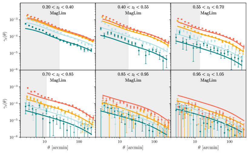
Figure 2: Tangential shear measurements of the redMaGiC (top) and MagLim (bottom) sample together with the best-fit theory line from the DES Y3 3$\times$2pt results. The shaded regions are excluded from the analysis; note that this includes the complete 5th and 6th MagLim lens redshift bins.

Source redshift bin	$\left<e_{1}\right>$	$\left<e_{2}\right>$
1	$3.22\times 10^{-4}$	$1.60\times 10^{-4}$
2	$3.36\times 10^{-4}$	$3.74\times 10^{-5}$
3	$3.77\times 10^{-4}$	$8.75\times 10^{-6}$
4	$4.06\times 10^{-4}$	$-2.68\times 10^{-5}$

Table 2: Mean weighted ellipticity per each component. We subtract these values from the ellipticity components of each galaxy before computing the tangential shear.

III.2 Lens-source clustering: Boost factors

The model prediction for $\gamma_{t}$ assumes the mean $n(z)$ of the relevant lens and source bins, but does not account for the fact that source galaxies are preferentially located near lens positions due to the clustering between them whenever they overlap in redshift. There are several implications of this “lens-source clustering” which we explore here and in Sec. (V). Most notably, it leads to an excess number of lens-source pairs compared to what would be expected from the mean number densities. Because these pairs are physically nearby, the sources are unlensed, and the estimator in Eq. (2) is biased in a scale-dependent way compared to the theoretical prediction for $\gamma_{t}$. The impact of these excess lens-source pairs is an additional factor related to the projected lens-source correlation function, $\omega_{LS}(\theta)$. There are two possible approaches to remove this effect:

• Model the lens-source correlation function with sufficient accuracy for the scales under consideration, including the potential impact of nonlinear bias and magnification.

• Apply a “boost” factor to correct for the decrease of the measured lensing signal in the presence of lens-source clustering by measuring the excess of sources around tracers compared to random points as a function of scale, for every tracer-source bin combination. This was suggested for the first time in Sheldon et al. (2004) and has since then been used in several analyses, such as in Mandelbaum et al. (2005), Mandelbaum et al. (2006), Miyatake et al. (2015), Singh et al. (2017), Luo et al. (2018), Amon et al. (2018), Singh et al. (2020b), Blake et al. (2020), becoming part of the standard estimator for galaxy-galaxy lensing analyses. As demonstrated below, this approach is equivalent to using an unbiased estimator normalized using random positions rather than lens positions.

In this work we choose to correct for this effect using the boost factors since they are both accurate and easy to implement on photometric data. We can express the boost factors in terms of standard estimators for galaxy clustering and $\gamma_{t}$. We can rewrite the simplest standard tangential shear estimator from Eq. (2) with no boost factors (no bf) as

$$\gamma_{t,\text{no bf}}\,(\theta)=\left(\frac{\sum_{l}w_{l}}{\sum_{r}w_{r}}\frac{{\sum_{RS}w_{RS}(\theta)}}{{\sum_{LS}w_{LS}(\theta)}}\right)\left(\frac{\sum_{r}w_{r}}{\sum_{l}w_{l}}\frac{\sum_{LS}w_{LS}\,e_{t,LS}(\theta)}{\sum_{RS}w_{RS}(\theta)}\right),$$ (3)

where $w_{RS}=w_{r}\,w_{s}$ is the weight associated with each random-source pair, with $w_{r}=1$ for all random points. The second factor on the right-hand side of the equation is what our tangential model predicts when using the mean $n(z)$ across the survey footprint (including relevant higher-order effects as discussed in V). The first factor, which accounts for the excess unlensed sources, defines the inverse of the boost factor $B(\theta)$ and is just a simple version of the projected correlation function between lenses and sources $\omega_{LS}(\theta)$:

$$B(\theta)=1+\omega_{LS}(\theta)\equiv\frac{\sum_{r}w_{r}}{\sum_{l}w_{l}}\frac{{\sum_{LS}w_{LS}(\theta)}}{{\sum_{RS}w_{RS}(\theta)}},$$ (4)

The ratio between the sum of random points weights and lens galaxies weights normalizes the boosts accounting for the fact that the sample of random points is usually larger than the sample of lenses to decrease shot noise. We show the measured boost factors in Fig. 3 for each lens-source combination. They produce a maximum correction of $\sim 10\%$ at the smallest measured angular scale, and of $\sim 2\%$ at the smallest scale used in the 3$\times$2pt cosmological analysis (6 Mpc/$h$). We estimate the uncertainty of the boost factors using the jackknife method described in Sec. III.6.

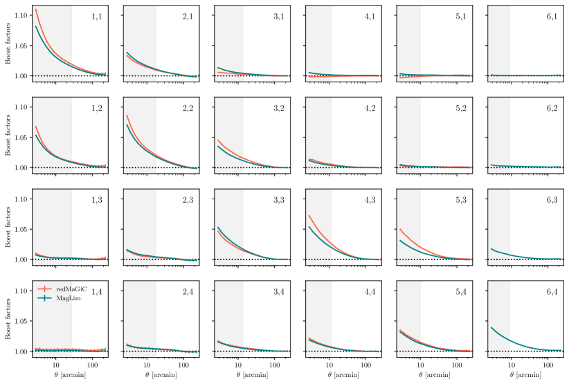
Figure 3: Boost factor measurements for both lens samples with uncertainties from the jackknife method. Shaded regions correspond to scales below 6 Mpc/$h$ excluded for the galaxy-galaxy lensing part of the 3$\times$2pt analysis. Note that some of the scales below 6 Mpc/$h$ are used for the shear-ratio (SR) analysis, see Sánchez, Prat et al. (2021) for the exact SR scale cuts.

A major advantage of measuring the boost factors in this way is that it is independent of the estimated redshift distributions, and in particular of the tails of the redshift distributions, which need to be very well characterized to measure the overlap between lenses and sources accurately. Also, the boost factors measured from data naturally include all effects that can impact lens and source pair counts, such as lens and source magnification. In this analysis we model lens magnification but we do not include source magnification, which is a much smaller effect for galaxy-galaxy lensing. Also, we discuss the general impact of both lens and source magnification on galaxy-galaxy lensing in Sections IV.3 and V.3, respectively. The estimator for the tangential shear that includes boost factors (bf) to match the theoretical prediction given some mean $n(z)$ is:

$$\gamma_{t,\text{bf}}\,(\theta) =B(\theta)\ \gamma_{t,\text{no bf}}=\frac{\sum_{r}w_{r}}{\sum_{l}w_{l}}\frac{\sum_{LS}w_{LS}\,e_{t,LS}(\theta)}{\sum_{RS}w_{RS}(\theta)}$$ (5)

which in the end is just the usual tangential shear estimator normalized by the sum of random-source weights instead of lens-source weights, taking into account the ratio between the total sum of weights for the whole sample of random points and lenses.

The $\Delta\chi^{2}$ between the tangential shear estimator with boost factors and without them is $\sim$9.8 from MagLim ($\sim$6.6 for redMaGiC) for the whole range of scales and $\sim$0.2 ($\sim$0.1) for the scales used in the 3$\times$2pt combination (above 6 Mpc/$h$), so it is negligible for the large scales. We still apply the boost factor correction at all scales to be consistent with the small scales used in the shear-ratio analysis where the correction becomes more important. We show the impact of the boost factor correction on the datavector in Fig. 4.

III.3 Random point subtraction

One advantage of galaxy-shear cross-correlations over shear-shear correlations is that additive shear systematics average to zero in the tangential coordinate system. However, this cancellation only occurs when sources are distributed isotropically around the lens and additive shear is spatially constant, two assumptions that are not accurate in practice, especially near the survey edge or in heavily masked regions, where there is a lack of symmetry on the source distribution around the lens. To remove additive systematics robustly, we also measure the tangential shear around random points. Such points have no net lensing signal (see Appendix C), yet they sample the survey edge and masked regions in the same way as the lenses. Another advantage of removing the tangential shear measurement around random points is that it removes a term in the covariance due to performing the measurement using the over-density field instead of the density field, as was found in Singh et al. (2017). Our estimator including boost factors and random point subtraction becomes:

$$\gamma_{t}(\theta)=\frac{\sum_{r}w_{r}}{\sum_{l}w_{l}}\frac{\sum_{LS}w_{LS}\,e_{t,LS}(\theta)}{\sum_{RS}w_{RS}(\theta)}-\frac{\sum_{RS}w_{RS}\,e_{t,RS}(\theta)}{\sum_{RS}w_{RS}(\theta)}$$ (6)

Note we only apply the boost factor correction to the lens term, since only the lenses are clustered with the sources.

In this work we use 40 times as many random points as the number of lens galaxies per tomographic bin for each galaxy sample. We have tested that this number of random points is enough by using two independent sets of random points with $\times$40 randoms each and comparing the results. We have performed this test using the Buzzard (DeRose et al., 2021b, 2019; Wechsler et al., 2021; DeRose et al., 2021a; Becker, 2013) DES Y3 $N$-body simulations using a redMaGiC-like sample. The $\Delta\chi^{2}$ between these two measurements in the simulations is $\sim 16$ for the whole range of scales (400 data points) and $\sim 7.5$ for the scales used in the 3$\times$2pt combination above 6 Mpc/$h$ (248 data points). This level of added noise is not significant for our analysis according to Friedrich et al. (2021). We also show the difference between these two measurements compared with the fiducial uncertainties in Fig. 4.

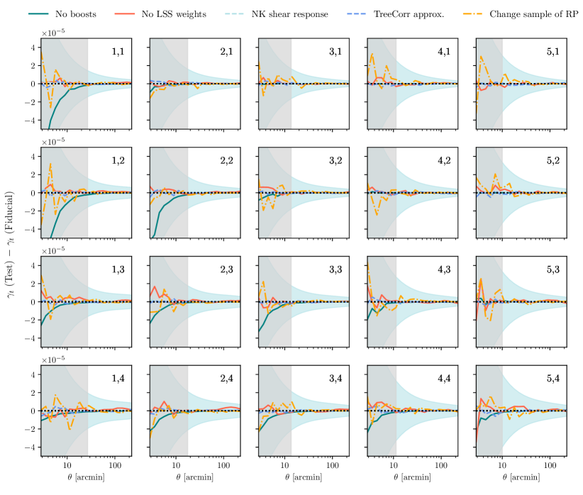
Figure 4: Impact of different effects on the tangential shear estimator, for the redMaGiC sample. The fiducial uncertainties (but without including the point-mass marginalization) are shown shaded in light blue. The scale cuts used in the DES Y3 3$\times$2pt analysis (6 Mpc/$h$) are represented by the gray shading. No boosts: Not including the boost factor correction to the estimator, see Sec. III.2. No LSS weights: Not applying the weights to the lens galaxies to correct for observing conditions, see Sec. VI.3. NK shear response: Using the scale dependent shear responses instead of the mean response, see more details in Sec. III.4.2. TreeCorr approx.: Impact of the approximation TreeCorr uses to increase speed, see Sec. III.6. Change sample of RP: Compares the random-subtracted fiducial measurements using a sample of random points 40$\times$ larger than the number of lenses, with measurements using another sample of random points, see Sec. III.3.

	$\Delta\chi^{2}$ redMaGiC				$\Delta\chi^{2}$ MagLim
	All scales	$R<6h^{-1}$Mpc	$R>6h^{-1}$Mpc		All scales	$R<6h^{-1}$Mpc	$R>6h^{-1}$Mpc
Boost factor (Included)	6.6	6.5	0.1		9.8	9.8	0.2
LSS weights (Included)	4.2	1.1	3.1		5.4	0.69	4.8
NK shear response	0.0078	0.0076	0.0002		0.0071	0.0068	0.0006
TreeCorr Approximation	$\sim$1.5	$\sim$0.5	$\sim$1		$\sim$1.5	$\sim$0.5	$\sim$1

Table 3: Difference in $\chi^{2}$ of several measurement effects with respect to the fiducial measurements, using the CosmoLike theoretical covariance (without point-mass marginalization). The impact of these effects is also shown in Fig. 4 for the redMaGiC sample. The redMaGiC datavector has 400 data points, 152 at small scales (below $6h^{-1}$Mpc) and 248 at large scales (above $6h^{-1}$Mpc). The MagLim one has 480 data points, 176 at small angular scales and 304 at large scales.

III.4 Shape measurement calibration: Response factors

In this work we use the Metacalibration shape catalog (Huff & Mandelbaum, 2017; Sheldon & Huff, 2017), which has the advantage of being able to self calibrate the mean shear measurement using the data themselves, via the so-called response factor. In this section we describe the methodology to correct the mean shear, and in particular the mean tangential shear, for potential biases that arise in the process of using the mean of noisy and model-dependent individual ellipticity measurements as an estimator for the mean shear. The two-component ellipticity can be written as a function of the two-component shear $\bm{e}(\bm{\gamma})$ and Taylor-expanded around zero shear as:

$$\bm{e}(\bm{\gamma})=\left.\bm{e}\right|_{\gamma=0}+\left.\frac{\partial\bm{e}}{\partial\bm{\gamma}}\right|_{\gamma=0}\bm{\gamma}+...\equiv\left.\bm{e}\right|_{\gamma=0}+\bm{R}_{\gamma}\bm{\gamma}+...\,,$$ (7)

where we have defined the shear response $R_{\gamma}$ as the first derivative of the ellipticity with respect to shear. This quantity is useful since it allows us to obtain the unbiased relation between the mean ellipticity and the mean shear at first order, assuming the intrinsic ellipticity of galaxies are randomly oriented. This can be seen by averaging the equation above over an ensemble of galaxies:

$$\left<\bm{e}\right>\approx\left<\bm{R}_{\gamma}\bm{\gamma}\right>,$$ (8)

and inverting the relation:

$$\left<\bm{\gamma}\right>\approx\left<\bm{R}_{\gamma}\right>^{-1}\left<\bm{e}\right>.$$ (9)

For the tangential shear, we can apply the tangential rotation defined in Eq. (1) to each of the quantities, yielding:

$$\left<\gamma_{t}\right>\approx\left<\bm{R}_{\gamma_{t}}\right>^{-1}\left<e_{t}\right>.$$ (10)

Next we describe how to compute the response factors. The shear response can be measured for each galaxy by artificially shearing the images in a particular direction $j$ and remeasuring the ellipticity:

$$R_{\gamma,i,j}=\frac{e_{i}^{+}-e_{i}^{-}}{\Delta\gamma_{j}}$$ (11)

where $e_{i}^{+}$, $e_{i}^{-}$ are the ellipticity measurements on the component $i$ made on an image sheared by $+\gamma_{j}$ and $-\gamma_{j}$, respectively, and $\Delta\gamma_{j}=2\gamma_{j}$. In this work we use $\Delta\gamma_{j}=0.02$. Also, notice that $R_{\gamma,i,j}$ is a $2\times 2$ matrix and if the estimator of the ellipticity is unbiased the mean response matrix will be equal to the identity matrix.

III.4.1 Selection response

Besides the shear response correction described above, in the Metacalibration  framework, when making a selection on the original full catalog using a quantity that could modify the distribution of ellipticities, for instance a cut in redshift, it is possible to correct for selection effects via the so-called selection response, defined as:

$$\left<R_{S,i,j}\right>=\frac{\left<e_{i}\right>^{S_{+}}-\left<e_{i}\right>^{S_{-}}}{\Delta\gamma_{j}},$$ (12)

where $\left<e_{i}\right>^{S_{+}}$ represents the mean of the $i$-component of ellipticities measured on images without applied shearing in component $j$, over the group of galaxies selected using the parameters extracted from positively sheared images. $\left<e_{i}\right>^{S_{-}}$ is the analogue quantity for negatively sheared images. In the absence of selection biases, $\left<\bm{R}_{S}\right>$ would be zero. Otherwise, the full response is given by the sum of the shear and selection response:

$$\left<\bm{R}\right>=\left<\bm{R}_{\gamma}\right>+\left<\bm{R}_{S}\right>.$$ (13)

In this work we compute the selection response due to selection effects produced when dividing the galaxies into tomographic bins. The results of the mean response for each redshift bin are shown in Table 4.

$z_{s}$-bin	$\left<R\right>$	$\left<R_{\gamma}\right>$	$\left<R_{S}\right>$	$\left<R_{11}\right>$	$\left<R_{22}\right>$
1	0.7682	0.7636	0.0046	0.7669	0.7695
2	0.7266	0.7182	0.0083	0.7258	0.7273
3	0.7014	0.6887	0.0126	0.7006	0.7022
4	0.6299	0.6154	0.0145	0.6296	0.6302

Table 4: $\left<R\right>$ is the mean total Metacalibration response for each of the source tomographic bins. $\left<R_{\gamma}\right>$ is the mean shear response and $\left<R_{S}\right>$ the mean selection response. $R_{11}$ and $R_{22}$ are the diagonal elements of the mean response matrix, i.e., the mean response for each ellipticity component with the artificial shear applied in the same direction.

III.4.2 Response factor approximations for the tangential shear estimator

In order to simplify the calculation of the response factors and reduce the computing time, in this work we make use of two approximations:

• We assume the correction to be independent of the relative orientation of galaxies, i.e., we do not rotate the response matrix as it is done with the shears, which are projected to the tangential component. That means we do not apply Eq. (10), which would be the exact correction. We find it is safe to not project the response matrix since the difference between the values for each of the two diagonal elements $R_{11}$ and $R_{22}$ is between 0.01% and 0.1%, as shown in Table 4. Then, since the response matrix is diagonal to good approximation, we just take the average of these components for each galaxy and therefore the response correction becomes just a scalar instead of a matrix:

  $$R\approx\frac{R_{11}+R_{22}}{2}$$ (14)

• We assume it is sufficient to average the individual scalar responses over the ensemble of galaxies for each redshift bin, instead of over the source galaxies used in each angular bin, specifically that is assuming that:

  $$\left<R\right>=\frac{\sum_{s}w_{s}R_{s}}{\sum_{s}w_{s}}\approx\frac{\sum_{LS}w_{LS}R_{LS}(\theta)}{\sum_{LS}w_{LS}(\theta)}\approx\frac{\sum_{RS}w_{RS}R_{RS}(\theta)}{\sum_{RS}w_{RS}(\theta)}$$ (15)

  where $R_{s}$ is the scalar response for each source galaxy $s$ as computed in Eq. (14), not to be confused with the selection response $R_{S}$. $LS$ and $RS$ are the same summation indexes used in Sec. III.2 and Sec. III.3, running over all the lens-source pairs or random-source pairs respectively, in each angular bin $\theta$. If instead we wanted to perform the exact correction averaging the response of the galaxies that fall into each angular bin, the tangential shear estimator would take this form:

  $$\gamma_{t}(\theta)=B(\theta)\frac{\sum_{LS}w_{LS}\,e_{t,LS}(\theta)}{\sum_{LS}w_{LS}R_{t,LS}(\theta)}-\frac{\sum_{RS}w_{RS}\,e_{t,RS}(\theta)}{\sum_{RS}w_{RS}R_{t,RS}(\theta)}$$ (16)

  We find the $\Delta\chi^{2}$ between the measurement using Eq. (16) (except applying the tangential rotation to the response) and the fiducial estimator using the mean response written in Eq. (18) to be $\sim$0.01 for the whole range of scales for the MagLim sample ($\sim$0.0006 for large scales above 6 Mpc/$h$) and therefore negligible for our analysis. See Table 3 for the rest of $\Delta\chi^{2}$ results. A visualization of this test is also shown in Fig. 4.

III.5 Final tangential shear estimator

Using the response approximations described above, the application of the boost factors and the random point subtraction, the complete tangential shear estimator used in this analysis can be written as:

$$\gamma_{t}(\theta)=\frac{1}{\left<R\right>}\left[B(\theta)\frac{\sum_{LS}w_{LS}\,e_{t,LS}(\theta)}{\sum_{LS}w_{LS}(\theta)}-\frac{\sum_{RS}w_{RS}\,e_{t,RS}(\theta)}{\sum_{RS}w_{RS}(\theta)}\right]$$ (17)

where $\left<R\right>$ is the weighted average Metacalibration  response in the corresponding source redshift bin, i.e. $\left<R\right>=\sum_{s}w_{s}R_{s}/\sum_{s}w_{s}$. Expanding the boost term, our final estimator can alternatively be written as

$$\gamma_{t}(\theta)=\frac{1}{\left<R\right>}\left[\frac{\sum_{r}w_{r}}{\sum_{l}w_{l}}\frac{\sum_{LS}w_{LS}\,e_{t,LS}(\theta)}{\sum_{RS}w_{RS}(\theta)}-\frac{\sum_{RS}w_{RS}\,e_{t,RS}(\theta)}{\sum_{RS}w_{RS}(\theta)}\right],$$ (18)

The tangential shear measurements using this estimator are shown in Fig. 2.

III.6 Measurement pipeline technical details and code comparison

In this section we specify the details of our fiducial measurement pipeline. This includes the description of pertinent optimizations we have used to reduce the memory and increase the speed of our code, given the large number of lens-source (and especially random-source) pairs that can be found in the DES Y3 samples. We also describe the details of the successful comparison of the results of the fiducial code (internally referred to as xcorr) with an independent pipeline (internally referred to as 2pt_pipeline).

Our measurement pipeline is based on the software package TreeCorr (Jarvis et al., 2004) to measure the different two-point correlation functions present in Eq. (17). Specifically, we use the NGCorrelation class from TreeCorr to perform the shape-position correlations. We set the bslop parameter from TreeCorr to zero in all our measurements, which ensures there is no variance between different users in how galaxy pairs are assigned into angular bins. Both for performance optimization purposes and to obtain a Jackknife covariance, we split the lens galaxies and random points into 150 regions using the kmeans algorithm, which given the footprint area of $\sim 4150$ deg² yields regions of approximately $5\mathrm{deg}^{2}$ or $\sim 300$ arcmin of length assuming a square geometry (the largest angular scale we measure is 250 arcmin). We then call TreeCorr to perform the NGCorrelation between each of the lens (and random) patches and selected sources around each lens patch. Once we have the measurement in each of the lens and random patches, we sum all the correlations appropriately following Eq. (17) to obtain our fiducial tangential shear measurements. We also use the measurements in the different patches to obtain a Jackknife covariance for the boost factor measurement and the corresponding diagonal uncertainties used in Figure 3.

The selection of sources around each lens patch significantly reduces the amount of memory needed to complete this calculation, and is achieved by building a healpix grid of nside=4 for the source galaxies and selecting the pixel in this grid corresponding to the center of each lens patch together with all its surrounding healpix pixels. Then, we apply a further mask using a matching function from Astropy (Astropy Collaboration, 2018) to only select source galaxies that are within a distance of 1.5 times the maximum angular separation we are interested in measuring. We do this in a two-step process to minimize the amount of memory used and increase speed, since the Astropy matching is more precise but requires more memory and is slower. We have tested that using this optimization does not result in any loss of lens-source pairs. However, note that if a different catalog is given to TreeCorr to build the tree, even if the eventual number of pairs used for the measurements is exactly the same, this will result in a small difference in the measurements. This can be avoided using the brute force option within TreeCorr, which is nonetheless much slower. This approximation produces a $\Delta\chi^{2}\sim 1$ for our setup. We also show the impact of using this approximation in Fig. 4, where we can visualize the difference between the two tangential shear measurements. Due to the increase in speed and decrease in memory we achieve using this approximation, and the very low significance of the effect, we use it in our fiducial measurements.

We have compared the results of our fiducial measurement pipeline applied and obtained a $\Delta\chi^{2}\lesssim 1$ for both galaxy samples, with 400 data points for redMaGiC (or 480 for MagLim). We consider this result successful and also want to take this opportunity to stress the importance of comparing measurement pipelines in future analyses as well, given that in our analysis it was very effective in identifying bugs and sources of error we were not initially considering. After this code comparison we compared with a third pipeline (with the caveat that is also based on TreeCorr) and also obtained a $\Delta\chi^{2}\lesssim 1$ to both of our previous pipelines. The reason for these remaining differences is that the different pipelines were building the “trees” within TreeCorr in a different way.

In this whole section all the quoted $\Delta\chi$’s are computed using the theoretical covariance without including the point-mass marginalization, therefore the real impact of these effects on the 3$\times$2pt cosmological analysis could actually be smaller given the effective increase of the covariance due to point-mass marginalization, which is especially important at small and intermediate scales, see Sec IV.2 for more details.

III.7 Blinding

In this work and within the 3$\times$2pt analysis we use a two-level blinding scheme that consists of having:

1. Blinding at the catalog level: An unknown multiplicative factor has been applied to the ellipticity measurements of all the source galaxies used in this work until the moment of unblinding.

2. Blinding at the two-point level: Using the method described in Muir et al. (2020) we modify the tangential-shear two-point correlation function measurements, effectively shifting them by a cosmology-dependent factor. The shifted, and thus blinded, two-point function has the property of preferentially looking like the correlation function of another cosmological model.

More details on the blinding criteria can be found in DES Collaboration (2022).

IV Modeling the tangential shear

The tangential shear is the main measurement used in this paper as detailed in the previous section, and here we describe how we model it in this work and within the DES Y3 3$\times$2pt cosmological analysis. See also the DES Y3 3$\times$2pt methodology paper (Krause et al., 2021) for further descriptions and the modeling of the other two-point correlation functions. We start by describing the basic modeling scheme, and then discuss the addition of several effects to our model, such as the removal of small scale information using the point-mass marginalization scheme, lens magnification, intrinsic alignments and a description of the galaxy bias model. At the end we detail the comparison of our fiducial modeling pipeline with an independent code.

IV.1 Basic tangential shear modeling

The tangential shear two-point correlation function is a transformation of the 2D galaxy-matter angular cross-power spectrum $C_{gm}$, which in this work we perform using the curved sky projection as detailed later in Eq. (24). First we will describe how we can model $C_{gm}$ and express it as a projection of the 3D galaxy-matter power spectrum $P_{gm}$. For a lens redshift bin $i$ and a source redshift bin $j$, under the Limber approximation (Limber, 1953; LoVerde & Afshordi, 2008) and assuming a flat Universe cosmology we can write:

$$C_{gm}^{ij}(\ell)=\int d\chi\frac{N_{l}^{i}(\chi)\,q_{s}^{j}(\chi)}{\chi^{2}}P_{gm}\left(k=\frac{\ell+1/2}{\chi},z(\chi)\right)\,,$$ (19)

where $k$ is the 3D wavenumber, $\ell$ is the 2D multipole moment, $\chi$ is the comoving distance to redshift $z$, and $N_{l}^{i}(\chi)$ and $q_{s}^{j}(\chi)$ are the window functions of the given lens and source populations of galaxies used in Limber’s approximation, which holds if the 3D galaxy overdensity field of the lenses and the 3D matter overdensity field at the redshift of the source galaxies vary on length scales much smaller than the typical length scale of their respective window functions in the line of sight direction. The lens window function is defined as:

$$N_{l}^{i}(\chi)=\frac{n^{i}_{l}\,(z)}{\bar{n}^{i}_{l}}\frac{dz}{d\chi},$$ (20)

where $n^{i}_{l}$ is the lens redshift distribution and $\bar{n}^{i}_{l}$ is the mean number density of the lens galaxies. The lensing window function of the source galaxies is:

$$q_{s}^{j}(\chi)=\frac{3H^{2}_{0}\Omega_{m}}{2c^{2}}\frac{\chi}{a(\chi)}g(\chi)$$ (21)

where $a$ is the scale factor and $g(\chi)$ is the lensing efficiency kernel:

$$g(\chi)=\int_{\chi}^{\chi_{\text{lim}}}d\chi^{\prime}\frac{n^{j}_{s}\,(z)\,dz/d\chi^{\prime}}{\bar{n}^{j}_{s}}\frac{\chi^{\prime}-\chi}{\chi^{\prime}}$$ (22)

with $n_{s}^{j}(z)$ being the redshift distribution of the source galaxies, $\bar{n}^{j}_{s}$ the mean number density of the source galaxies and $\chi_{\mathrm{lim}}$ the limiting comoving distance of the source galaxy sample.

Ultimately we want to relate the galaxy-matter power spectrum to the matter power spectrum. In our fiducial model we assume that lens galaxies trace the mass distribution following a simple linear biasing model ($\delta_{g}=b\>\delta_{m}$), so the galaxy-matter power spectrum relates to the matter power spectrum by a multiplicative galaxy bias factor:

$$P^{ij}_{gm}=b^{i}P^{ij}_{mm}.$$ (23)

We summarize the tests we have performed to make this modeling choice in Sec. V.1, and see Pandey et al. (2021) for an extended description. We compute the non-linear matter power spectrum using the Takahashi et al. (2012) version of Halofit and the linear power spectrum is computed with CAMB.

IV.1.1 Angular bin averaging and full sky projection

Given the galaxy-matter angular power spectra we can obtain the tangential shear quantity via the following transformation on the curved sky, as a function of angular scale $\theta$ between lens and source galaxies:

$$\gamma_{t}^{ij}(\theta)=\sum_{\ell}\frac{2\ell+1}{4\pi\ell(\ell+1)}P^{2}_{\ell}(\cos\theta)\,C^{ij}_{gm}(\ell)~{},$$ (24)

where $P_{\ell}^{2}$ are the associated Legendre polynomial. We calculate the correlation functions within an angular bin $[\theta_{\rm min},\theta_{\rm max}]$, by carrying out the average over the angular bin, i.e., replacing $P_{\ell}^{2}(\cos\theta)$ with their bin-averaged function $\overline{P^{2}_{\ell}}$, from Fang et al. (2020):

$$\overline{P^{2}_{\ell}}\left(\theta_{\rm min},\theta_{\rm max}\right)\equiv\frac{\int_{\cos\theta_{\rm min}}^{\cos\theta_{\rm max}}dx\,P^{2}_{\ell}(x)}{\cos\theta_{\rm max}-\cos\theta_{\rm min}}=$$

$$=\frac{\left[\left(\ell+\frac{2}{2\ell+1}\right)P_{\ell-1}(x)+(2-\ell)\,x\,P_{\ell}(x)-\frac{2}{2\ell+1}P_{\ell+1}(x)\right]^{\cos{\theta_{\rm max}}}_{\cos{\theta_{\rm min}}}}{\cos\theta_{\rm max}-\cos\theta_{\rm min}}$$ (25)

We show the effect of including the full-sky transform and the bin-averaging implementation, given they are both new in the Y3 modeling with respect to the Y1 one, versus using the flat-sky approximation and no averaging in scales within each angular bin in Fig. 5.

Note there is an additional effect from the variation in the pair counts due to the survey geometry not taken into account in Eq. (24), which we have found negligible for the DES Y3 analysis setup. See App. B for more details.

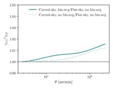
Figure 5: Illustration of the curved sky and angular bin averaging effect to the tangential shear modeling. In the DES Y3 3$\times$2pt cosmological analysis we model the tangential shear using the curved sky transform (vs the flat sky approximation, used in the DES Y1 3$\times$2pt analysis for instance) and we properly average within the range of scales falling in each angular bin (vs just picking one value in the middle of the bin, also employed in the Y1 modeling). The effects are shown for the first lens tomographic bin and second source tomographic bin, but they are not very dependent on redshift.

IV.2 Removing small-scale information: Point-mass marginalization

The tangential shear is a non-local quantity. This can be appreciated expressing the tangential shear of a single lens-source pair as a function of the excess surface mass density $\Delta\Sigma$:

$$\gamma_{t}\,(\theta)=\frac{\Delta\Sigma\,(\theta)}{\Sigma_{\mathrm{crit}}},$$ (26)

where $\Sigma_{\mathrm{crit}}$ is a geometrical factor that depends on the angular diameter distances to the lens galaxy $D_{l}$, the one between the lens and the source $D_{ls}$ and the one to the source galaxy $D_{s}$, and is defined as:

$$\Sigma_{\mathrm{crit}}^{-1}(z_{\rm l},z_{\rm s})=\frac{4\pi G}{c^{2}}\frac{D_{ls}\,D_{l}}{D_{s}}\qquad\mathrm{if}z_{s}>z_{l},$$ (27)

and zero otherwise. Also, $\Delta\Sigma$ can be expanded as the difference between the mean surface mass density below a certain angular scale $\theta$ and the surface mass density at this given scale:

$$\Delta\Sigma\,(\theta)=\overline{\Sigma}\,(<\theta)-\Sigma\,(\theta),$$ (28)

where the non-locality of the tangential shear quantity becomes apparent, since the tangential shear defined at some $\theta$ value will always carry information of all the scales below this value. This is the reason the scale cuts in the DES Y1 3$\times$2pt cosmological analysis were higher for the galaxy-galaxy lensing part (12 Mpc/$h$) than for the galaxy clustering part (8 Mpc/$h$). In this analysis we would need to apply an even more stringent cut due to the smaller statistical uncertainties. Alternatively, it is possible to localize the tangential shear measurement. For instance Park et al. (2021) suggested applying a linear transformation to the tangential shear observable to remove this non-locality. In this work and in the context of the 3$\times$2pt DES Y3 cosmological analysis we decide to account for this instead following MacCrann et al. (2020). Internal tests for the Y3 analysis have shown both methods yielding very similar results in the recovered cosmological constraints. MacCrann et al. (2020) proposes to analytically marginalize over a point-mass (PM) scaling as $R^{-2}$ with physical separation $R$ between the lens and the source galaxy, including some additional terms in the tangential shear covariance coming from the uncertainty in the model prediction of galaxy-matter correlation function below a given scale. Starting by expressing the point-mass term as an addition to the tangential shear model for a given lens redshift bin $i$ and source redshift bin $j$ as a function of angular separation:

$$\gamma_{t}^{ij}\,(\theta)=\gamma_{t,\rm model}^{ij}\,(\theta)+\frac{A^{ij}}{\theta^{2}}\,,$$ (29)

where $A^{ij}$ is the following function:

$$A^{ij}=\int dz_{l}\int\ dz_{s}\ n^{i}_{l}(z)\ n^{j}_{s}(z)\ B^{i}(z_{l})\ \Sigma^{-1}_{\rm crit}(z_{l},z_{s})\ D^{-2}(z_{l})\,,$$ (30)

that depends on the point-mass $B^{i}$ we want to marginalize over. In general $B^{i}$ can evolve within the lens bin but given the tomographic binning scheme of our lens sample, we can assume the lens redshift bins are narrow enough so that we can approximate the previous equation to:

$$A^{ij} \approx B^{i}\int dz_{l}\int\ dz_{s}\ n^{i}_{l}(z)\ n^{j}_{s}(z)\ \Sigma^{-1}_{\rm crit}(z_{l},z_{s})\ D^{-2}(z_{l})$$ (31)

$$\equiv B^{i}\beta_{ij}$$ (32)

This is advantageous because in this case the $\beta_{ij}$ parameters can be naturally constrained from the data itself via implicit shear-ratio information. In other words, some of the constraining power of the tangential shear measurements, and in particular the geometrical information, is naturally used within the 3$\times$2pt combination to constrain the $\beta_{ij}$ parameters. Then, given the simple form of this contamination model (e.g. the scale dependence is not dependent on cosmology or the lens galaxy properties), this term can be analytically marginalized, i.e. we only need to add some terms to the tangential shear covariance matrix to effectively “remove” information below the angular scale $\theta$. We perform an analytic marginalization over all $B_{i}$, which can be done by adding the following terms to the original tangential shear covariance matrix $\mathbf{C}$ to become (Bridle et al., 2002; MacCrann et al., 2020):

$$\mathbf{C}^{+PM}_{ij\theta,i^{\prime}j^{\prime}\theta^{\prime}}=\left\{\begin{array}[]{ll}\mathbf{C}_{ij\theta,i^{\prime}j^{\prime}\theta^{\prime}}+\sigma^{2}_{B_{i}}\beta_{ij}/\theta^{2}\cdot\sigma^{2}_{B_{i}^{\prime}}\beta_{i^{\prime}j^{\prime}}/\theta^{\prime 2}\quad\mathrm{if}\ i=i^{\prime}\\ \mathbf{C}_{ij\theta,i^{\prime}j^{\prime}\theta^{\prime}}\qquad\qquad\qquad\qquad\quad\ \ \ \qquad\mathrm{if}\ i\neq i^{\prime}\end{array}\right.$$ (33)

under the narrow lens bin approximation. $\sigma^{2}_{B_{i}}$ is the width of the Gaussian prior on $B_{i}$ we want to marginalize over. In this work, we choose to adopt an uninformative prior and take the limit $\sigma^{2}_{B_{i}}\rightarrow\infty$. This is because for the chosen scale cuts of 6 Mpc/$h$ the point-mass is dominated by the 2-halo regime (see Appendix A from Pandey et al. 2021). In the 3$\times$2pt likelihood we will eventually need the inverse of the covariance matrix, instead of the covariance matrix itself. For the infinite prior case on $\sigma^{2}_{B_{i}}$, the inverse covariance matrix can be written as (MacCrann et al., 2020):

$$\mathbf{C}^{-1,+PM}=\mathbf{C}^{-1}-\mathbf{C}^{-1}\,\mathbf{V}\,(\mathbf{V}^{\mathbf{T}}\mathbf{C}^{-1}\,\mathbf{V})^{-1}\,\mathbf{V}^{\mathbf{T}}\,\mathbf{C}^{-1}$$ (34)

where $\mathbf{V}$ is a $N_{d}\times N_{\mathrm{lens}}$ matrix with the $i$th column being $\beta_{ij}/\theta^{2}$ and $N_{d}=N_{\theta}N_{\mathrm{lens}}N_{\mathrm{source}}$ being the number of elements in the datavector, $N_{\mathrm{lens}}$ the number of lens redshift bins and $N_{\mathrm{source}}$ the number of source tomographic bins. In Fig. 6 we show the change in the tangential shear inverse covariance matrix this produces. The changes in the inverse covariance are larger for the lower lens redshift bins due to the fact that at lower redshift a given angular scale corresponds to a larger physical scale than at higher redshift. The changes are also larger where the signal is bigger, i.e. for the lens-source combinations which are more separated in redshift. The S/N of the tangential shear measurements changes from $\sim$55 to $\sim$28 for the redMaGiC sample when the point-mass marginalization is applied to the inverse covariance. For MagLim the change in S/N is from $\sim$67 to $\sim$32. See also Pandey et al. (2021) for further details on the implementation of the point-mass marginalization in the DES Y3 3$\times$2pt analysis.

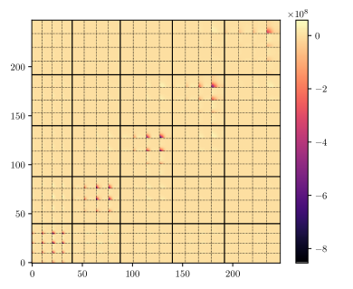
Figure 6: Difference in the tangential shear inverse covariance matrix between the cases assuming including the point-mass correlation or not, $\mathbf{C}^{-1,+PM}-\mathbf{C}^{-1}$. We illustrate this using the redMaGiC  sample and the >6 Mpc/$h$ scale cut. The difference is especially noticeable at small scales. Solid lines separate lens tomographic bins and dotted lines source tomographic bins.

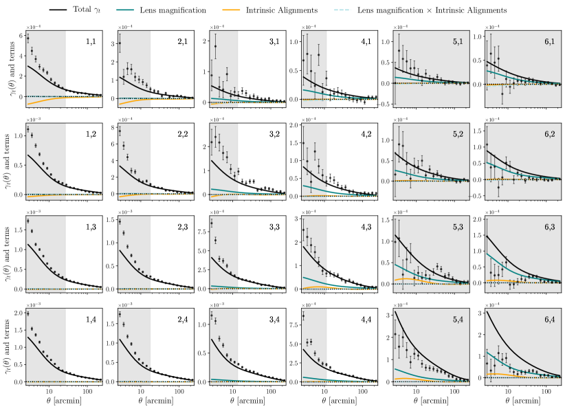
Figure 7: This plots shows the contribution from each of the components of our model at the best-fit values from the 3$\times$2pt result for the MagLim sample and the total model (black line), as obtained from Eq. (53). The contribution from the coupling of IA and lens magnification is very close to zero.

IV.3 Lens magnification

Lens magnification is the effect of magnification produced on the lens galaxy sample by the structure that is between the lens galaxies and the observer. In this section we describe how lens magnification affects the galaxy-galaxy measurements, how significant the effect is for the tangential shear probe, and how we model it. See Elvin-Poole, MacCrann et al. (2021) for further details regarding lens magnification within the DES Y3 analysis. This effect has also been studied for galaxy-galaxy lensing recently in Unruh et al. (2020).

In the weak gravitational lensing picture, besides having shape distortions described by the shear, the solid angle spanned by the image is changed compared to the solid angle covered by the source by the so-called magnification factor $\mu$. This change in solid angle can alter the number density of a given sample via two different mechanisms: (1) The number density decreases by a factor $\mu$ due the sky being locally stretched by the same factor and (2) Since the area increases but the surface brightness is conserved, the flux of individual galaxies rises, and some galaxies that would otherwise not have been detected pass the relevant flux threshold for a particular sample. These are two competing effects and the dominant one depends on the specifics of the galaxy sample. Then, to understand how lens magnification affects the tangential shear measurements, it is useful to express the observed density contrast for the lens sample as the sum of the intrinsic galaxy density contrast and the “artificial” one produced by lens magnification:

$$\delta_{g}^{\text{obs}}=\delta_{g}^{\text{int}}+\delta_{g}^{\text{mag}}.$$ (35)

Then we can make the assumption that the change in number density produced by magnification is proportional to the convergence (Elvin-Poole, MacCrann et al., 2021). In that case, we can write

$$\delta_{g}^{\text{mag}}(\theta)=C\kappa_{l}(\theta)\,,$$ (36)

where $\kappa_{l}$ is the convergence field at the lens redshift and $C$ is just a proportionality factor. At this point we can separate the area effect and the flux effect on the number density change: $C_{\mathrm{total}}=C_{\mathrm{area}}+C_{\mathrm{flux}}$, since it can be shown that $C_{\mathrm{area}}=-2$ (Elvin-Poole, MacCrann et al., 2021) while $C_{\mathrm{flux}}$ will depend on the sample. That is why this proportionality factor is usually written in the literature as $C_{\mathrm{total}}=2(\alpha-1)$, where $\alpha$ is a property of the sample and is equivalent to $C_{\mathrm{flux}}/2$. From now on we will adopt the “$\alpha$ notation” since it is more commonly used.

Lens magnification becomes relevant because the change in number density produced to the lens sample is correlated with the large scale structure that is between the lens galaxies and the observer. That means that for a given sample of lens galaxies, some lines-of-sight with, for instance, more matter between the lens galaxies and us could be over-sampled if $\alpha>1$, or down-sampled if $\alpha<1$, and the tangential shear measurement would be biased, as seen in the following equation:

$$\left<\delta_{g}^{\text{obs}}\gamma\right>=\left<\delta_{g}^{\text{int}}\gamma\right>+2(\alpha-1)\left<\kappa_{l}\gamma\right>=\left<\delta_{g}^{\text{int}}\gamma\right>+2(\alpha-1)\left<\kappa_{l}\gamma\right>.$$ (37)

The first term is just the usual galaxy-galaxy lensing signal, modeled for the tangential shear as given by Eqs. (19) and (24), and the additional lens magnification term is modeled in the following way before performing the projection to real space:

$$C_{mm}^{ij}(\ell)=\int d\chi\frac{q_{l}^{i}(\chi)\,q_{s}^{j}(\chi)}{\chi^{2}}P_{mm}\left(k=\frac{\ell+1/2}{\chi},z(\chi)\right)\,,$$ (38)

where the lensing window functions $q_{s}$ is defined in Eq. (21), and the analogous window function for the lens sample is given by $q_{l}$. The $i$ index represents the lens tomographic bin and $j$ the source one. The tangential shear model including the lens magnification term can be written as:

$$\gamma_{t}^{ij}(\theta)=\sum_{\ell}\frac{2\ell+1}{4\pi\ell(\ell+1)}P^{2}_{\ell}(\cos\theta)\left[C^{ij}_{gm}(\ell)+2(\alpha^{i}-1)C_{mm}^{ij}(\ell)\right]~{},$$ (39)

following the curved sky projection.

The $\alpha^{i}$ parameters have been carefully measured and extensively checked for both of the lens samples used in this work in Elvin-Poole, MacCrann et al. (2021), using realistic $N$-body simulations and Balrog image simulations (Everett et al., 2022). In this work and within 3$\times$2pt, we use the Balrog $\alpha^{i}$ estimates for the fiducial model, shown in Table 1.

IV.4 Intrinsic alignment model

In our tangential shear estimator from Eq. (18) we are averaging the ellipticity components to extract the shear. However the observed ellipticity of a galaxy $e^{\text{obs}}$, is related to the shear by (Seitz & Schneider, 1997):

$$e^{\text{obs}}=\frac{e^{\text{int}}+g}{1+g^{*}e^{\text{int}}}$$ (40)

where in this equation all variables are complex numbers, $g=\gamma/(1-\kappa)$ is the reduced shear and $g^{*}$ is the complex conjugate of $g$. In the weak lensing regime $\kappa\ll 1$, $\gamma\ll 1$ and we can then approximate the above equation to (we test this approximation in Sec. V.3.1):

$$e^{\text{obs}}\approx\gamma+e^{\text{int}}.$$ (41)

Thus, when averaging observed ellipticities we will only recover the shear if the intrinsic component of the ellipticity vanishes after averaging over many lens-source pairs. However this is not the case since the intrinsic component of the ellipticity, that is, the orientation of the source galaxies themselves, is correlated with the underlying large scale structure, and therefore with the lenses tracing this structure. We call this effect intrinsic alignments. This effect is only present in galaxy-galaxy lensing measurements if the lens and source galaxies overlap in redshift. To model galaxy intrinsic alignments, we employ the TATT (Tidal Alignment and Tidal Torquing, Blazek et al. 2019) and NLA (Non-linear linear alignment, Hirata & Seljak 2004) models.

It is typically assumed that the correlated component of intrinsic galaxy shapes is determined by the large scale cosmological tidal field $s$. The simplest relationship, which should dominate on large scales and for central galaxies, is when galaxy shapes align linearly with the background tidal field. This is what the NLA model is based on. More complex alignment processes, including tidal torquing, are relevant for determining the angular momentum of spiral galaxies and therefore their intrinsic orientation. The TATT model includes this additional component and is therefore better suited to describe the IA effects in a source sample that includes both red and blue galaxies. In nonlinear cosmological perturbation theory, we can write the intrinsic galaxy shape field, measured at the location of source galaxies, as an expansion of the density and tidal fields:

$$e^{\rm int}_{ij}=A_{1}s_{ij}+A_{1\delta}\delta s_{ij}+A_{2}s_{ik}s_{kj}+\cdots,$$ (42)

where only here we use the $i,j,k$ letters to label the indices for a spin-2 tensor (elsewhere they denote redshift bins). In this expansion, using only the first “linear” $A_{1}$ term corresponds to the NLA model (when the nonlinear power spectrum is used for density correlations), while using all three parameters corresponds to the TATT model. $A_{2}$ captures the quadratic contribution from tidal torquing and $A_{1\delta}$ can be seen as a contribution from “density weighting” the tidal alignment contribution: we only observe IAs where there are galaxies, which contributes this additional term at next to leading order. The relevant two-point correlation for galaxy-galaxy lensing is expressed through the galaxy-intrinsic power spectrum:

$$P_{gI}=bP_{\text{GI}},$$ (43)

where $b$ is the linear bias of the lens galaxies. While there are terms involving the correlation of IA and nonlinear galaxy bias, they are not included in our analysis here. These terms should be subdominant in the context of the TATT model and can be largely captured through the free $b_{TA}$ parameter defined in Eq. (48) (see, e.g., Blazek et al. 2015). $P_{\text{GI}}(k)$ is the lensing-intrinsic power spectrum which we will write for both the NLA and TATT models. For the NLA model, cross correlating the tangential component $e^{\rm int}$ from the first term of Eq. (42) with the lens galaxy density field we can write the lensing-intrinsic power spectrum:

$$P_{\text{GI}}(k,z)=\left<\delta_{g}e^{\rm int}_{t}\right>=A_{1}\left<\delta_{g}s_{E}\right>=A_{1}P_{mm}(k,z)\,,\quad[\textbf{NLA}]$$ (44)

where $s_{E}$ is the $E$-mode of the tidal field, and the last step is only possible because $P_{mm}$ is actually the same as $P_{ms_{E}}$ (but not in real space). Then, in the NLA model the IA power spectra are of the same shape as the matter power spectrum, but subject to a redshift-dependent rescaling, since we parametrize $A_{1}$ as $A_{1}(z)$, as defined below. For the TATT model, we perform the same expansion but now using all the terms from Eq. (42) to reach

$$\begin{split}P_{\text{GI}}(k,z)&=A_{1}\left<\delta_{g}s_{E}\right>+A_{1\delta}\left<\delta_{g}\,\delta s_{E}\right>+A_{2}\left<\delta_{g}\,s_{E}s_{E}\right>=\\ &=A_{1}P_{mm}(k,z)+A_{1\delta}P_{0|0E}(k,z)+A_{2}P_{0|E2}(k,z).\\ &\qquad\qquad\qquad\qquad\qquad\qquad\qquad\qquad\ \ [\textbf{TATT}]\end{split}$$ (45)

In this work, these terms are evaluated using FAST-PT (McEwen et al. 2016; Fang et al. 2017), as implemented in CosmoSIS. The full expressions for these power spectra can be found in Blazek et al. (2019) (see equations 37-39 and their appendix A). In our TATT model implementation $A_{1}$, $A_{2}$, and $A_{1\delta}$ are all redshift-dependent quantities, defined as:

$$A_{1}(z)=-a_{1}\bar{C}_{1}\frac{\rho_{\rm crit}\Omega_{\rm m}}{D(z)}\left(\frac{1+z}{1+z_{0}}\right)^{\eta_{1}}$$ (46)

$$A_{2}(z)=5a_{2}\bar{C}_{1}\frac{\rho_{\rm crit}\Omega_{\rm m}}{D^{2}(z)}\left(\frac{1+z}{1+z_{0}}\right)^{\eta_{2}}$$ (47)

$$A_{1\delta}(z)=b_{\mathrm{TA}}A_{1}(z),$$ (48)

where $\bar{C}_{1}$ is a normalisation constant, by convention fixed at a value $\bar{C}_{1}=5\times 10^{-14}M_{\odot}h^{-2}\mathrm{Mpc}^{2}$, obtained from SuperCOSMOS (see Brown et al. 2002). The denominator $z_{0}$ is a pivot redshift, which we fix to the value 0.62, the same as the value used in DES Y1 3$\times$2pt analysis. The dimensionless amplitudes $(a_{1},a_{2})$ and power law indices $(\eta_{1},\eta_{2})$ are free parameters in the TATT model, as well as the $b_{\text{TA}}$ parameter which accounts for the fact that the shape field is preferentially sampled in overdense regions.

Finally, the angular power spectrum of this IA contribution to galaxy-galaxy lensing is the relevant line-of-sight integral:

$$C_{gI}^{ij}(\ell)=\int d\chi\frac{N_{l}^{i}(\chi)\,N_{s}^{j}(\chi)}{\chi^{2}}P_{gI}\left(k=\frac{\ell+1/2}{\chi},z(\chi)\right)\,.$$ (49)

IV.4.1 Lens magnification $\times$ intrinsic alignments term

Similarly, there is the contribution from the correlation between lens magnification and source intrinsic alignments, which is also included in our fiducial model:

$$C_{mI}^{ij}(\ell)=\int d\chi\frac{q_{l}^{i}(\chi)\,N_{s}^{j}(\chi)}{\chi^{2}}P_{mI}\left(k=\frac{\ell+1/2}{\chi},z(\chi)\right)\,,$$ (50)

where $P_{mI}(k)=P_{\text{GI}}(k)$.

IV.5 Full tangential shear model

Our tangential shear fiducial model includes the lens magnification term, intrinsic alignments and cross-terms between lens magnification and IA and can be written as:

$$\begin{split}\gamma_{t}^{ij}(\theta)&=\sum_{\ell}\frac{2\ell+1}{4\pi\ell(\ell+1)}P^{2}_{\ell}(\cos\theta)\\ &\times\left[C^{ij}_{gm}(\ell)+2(\alpha^{i}-1)\,\left(C_{mm}^{ij}(\ell)+C_{mI}^{ij}(\ell)\right)+C_{gI}^{ij}(\ell)\right]~{},\end{split}$$

following the curved sky projection. We show the different contributions to our model in Fig. 7 with the free parameters evaluated at the 3$\times$2pt best-fit. For the IA parameters these correspond to $A_{1}=0.60,\,A_{2}=-0.16,\,\alpha_{1}=4.2,\,\alpha_{2}=3.8,\,b_{TA}=0.074$.

IV.6 Modeling pipeline technical details and code comparison

We use the CosmoSIS framework (Zuntz et al., 2015) to compute the theoretical modelling. The output from CosmoSIS has been compared with that of CosmoLike (Krause & Eifler, 2017) and reached an agreement of $\Delta\chi^{2}<0.1$ for the tangential shear part after scale cuts (>6 Mpc/$h$), which includes 248 points. The main differences between the two codes are that (1) CosmoSIS uses CAMB while CosmoLike uses CLASS, even though they are interchangeable for the DES Y3 3$\times$2pt analysis and (2) they use completely independent interpolation and integration schemes. Equivalently as for the measurement code, we stress the importance of performing such comparisons due to its effectiveness in identifying unexpected sources of error.

V Model validation

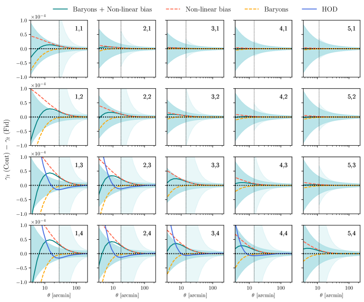
Figure 8: In this figure we show the difference between a simulated datavector contaminated with baryonic effects and non-linear galaxy bias with respect to the fiducial model (linear bias and Halofit non-linear matter power spectrum), and the equivalent difference for an HOD contaminated datavector using the model and results from Zacharegkas et al. (2022). The darker blue shaded regions indicate the uncertainties coming from the theory covariance without point-mass marginalization and the lighter ones including the point-mass marginalization. The dashed vertical black lines indicate the 6 Mpc/$h$ scale cuts. For more details see Sec V.1 and Sec. V.2

We now summarize the validation of the model for the galaxy-galaxy lensing signal described in Krause et al. (2021) for all the probes, by exploring and illustrating the impact of several modeling effects and choices that are relevant to galaxy-galaxy lensing. The fiducial model, which includes several effects such as intrinsic alignments or lens magnification, is described in Section IV. We explore the impact of several effects that are not included in the fiducial modeling, in particular those concerning non-linear galaxy bias modeling, baryonic effects on the power spectrum, the effect of reduced shear, source magnification and source clustering, and their interplay. Within the DES Y3 3$\times$2pt analysis, we have adopted the threshold of 0.3$\sigma$ changes in the $\Omega_{m}-S_{8}$ plane to decide whether some effect is significant enough to be included in the fiducial model before unblinding.

V.1 Galaxy bias model and baryonic effects

In our fiducial model we assume a linear galaxy bias relation between the matter power spectrum and the galaxy-matter cross-power spectrum, as written in Eq. (23). Also we do not include baryonic contributions to the non-linear matter spectrum we assume, given by the Takahashi et al. (2012) version from Halofit. In order to validate the applicability of both of these choices on scales greater than 6 Mpc/$h$, we analyze a simulated galaxy-galaxy lensing datavector that receives contributions from non-linearities due to non-linear galaxy biasing and baryonic feedback. The non-linear bias contribution to this contaminated simulated datavector was generated using 1-Loop Perturbation Theory (see Desjacques et al. 2018 for a review) at parameter values motivated from analyzing 3D statistics in MICE simulations (see Pandey et al. 2020 and Pandey et al. 2021 for more details). In Fig. 8 we illustrate the difference between the simulated datavector contaminated by baryonic effects and non-linear galaxy biasing as detailed above, and the fiducial vector, in comparison with the theoretical uncertainties, for illustrative purposes. We also show each of the effects separately in the same figure. When compared with the uncertainties without point-mass marginalization (with darker shade in that figure), we find they are not large enough to account for the differences between the two vectors, but once the point-mass marginalization is in place, the difference is always smaller than the uncertainties. Here the uncertainties from point-mass are obtained using a finite point-mass of $5\times 10^{13}M_{\odot}$ — otherwise the inverse covariance from Eq. (34) is not invertible. Then, this contaminated galaxy-galaxy lensing datavector is analyzed with the fiducial linear bias model in conjunction with galaxy clustering and cosmic shear. The bias in recovered cosmological parameters is less than 0.3$\sigma$ from the input truth values (see Pandey et al. 2021 and Krause et al. 2021 for more details).

V.2 Halo occupation distribution model

In Figure 8 we also show a simulated datavector produced with the halo occupation distribution model (HOD) developed in Zacharegkas et al. (2022). In their paper they fit the HOD model to tangential shear measurements of the redMaGiC and the MagLim sample from 0.25 to 250 arcmin, divided into 30 angular bins. In Zacharegkas et al. (2022) only the highest S/N lens-source redshift bins combinations are used to fit the HOD model, which are the ones where the lens and the source galaxies are more separated in redshift. In Fig. 8 the HOD line corresponds to their best-fit HOD model of the redMaGiC sample, which we compare with the fiducial model used in the 3$\times$2pt cosmological analysis. As expected, the HOD and the 3$\times$2pt model agree on large scales but they show strong deviations at smaller scales. Also note the data-informed HOD model shows smaller differences with respect to the fiducial model than the baryons + Non-linear bias contaminated data vector which has been used to define the scale cuts, validating it as a conservative choice.

V.3 Reduced shear, source magnification and source clustering

We now consider the impact of the reduced shear approximation, and the source magnification and source clustering effects, which are all connected to each other as well as to the lens magnification and IA terms which we described in Sec. IV.3 and Sec. IV.4 respectively. In this section we will write the contribution to position-shape correlations of all these effects. In Sec. V.3.1 we will describe in more detail the reduced shear approximation and the tests we have performed to validate it, and in Sec. V.3.2 we focus on source magnification and source clustering. This work has been performed following Krause et al. (2021), which studies second-order effects not only to galaxy-galaxy lensing but to the other correlation functions and where the full expressions for each of the effects can be found. Here we summarize their conclusions affecting the galaxy-galaxy lensing observable and illustrate some of the effects at the two-point function level. We also expand on the relation of the source magnification and source clustering effects with the tangential shear estimator presented in this work.

We can start by writing the observed lens galaxy density as we derived in Sec. IV.3, including the lens magnification term:

$$\delta_{g}^{\text{obs}}=\delta_{g}^{\text{int}}+\delta_{g}^{\text{mag}}=\delta_{g}^{\text{int}}+C_{l}\kappa_{l},$$ (51)

and then we can also write the observed ellipticity $e^{\text{obs}}$ as the following expression, which includes the higher-order effects of reduced shear, with a (1+$\kappa_{s}$) factor after using a Taylor expansion, where $\kappa_{s}$ is the convergence field at the redshift of the sources, intrinsic alignments produced by the intrinsic ellipticity $e^{\rm int}$, source clustering represented by $\delta_{s}$, source magnification $C_{s}\kappa_{s}$ (following the analogous notation as for lens magnification):

$$e^{\text{obs}}=(\gamma\,(1+\kappa_{s})+e^{\rm int})(1+\delta_{s}+C_{s}\kappa_{s}).$$ (52)

Correlating these two fields gives:

$$\begin{split}&\left<\delta_{g}^{\text{obs}}e^{\text{obs}}\right>=\left<(\delta_{g}^{\text{int}}+C_{l}\kappa_{l})(\gamma\,(1+\kappa_{s})+e^{\rm int})(1+\delta_{s}+C_{s}\kappa_{s})\right>=\\ &\qquad=\underbrace{\left<\delta_{g}^{\text{int}}\gamma\right>}_{\text{signal}}+\,\underbrace{C_{l}\left<\kappa_{l}\gamma\right>}_{\text{lens mag}}+\,\underbrace{\left<\delta_{g}^{\text{int}}e^{\rm int}\right>}_{\text{IA}}+\,\underbrace{C_{l}\left<\kappa_{l}e^{\rm int}\right>}_{\text{lens mag + IA}}+\\ &\qquad+\,\underbrace{\left<\delta_{g}^{\text{int}}e^{\rm int}\delta_{s}\right>}_{\text{IA + source clu }}+\,\underbrace{(1+C_{s})\left<\delta_{g}^{\text{int}}\gamma\kappa_{s}\right>}_{\text{red. shear or source mag }}\,+\,\underbrace{\left<\delta_{g}^{\text{int}}\gamma\delta_{s}\right>}_{\text{source clu}}\,+\\ &\qquad+\,\underbrace{C_{l}\,(1+C_{s})\left<\kappa_{l}\gamma\kappa_{s}\right>}_{\text{lens mag + (red. shear or source mag)}}+\,\underbrace{C_{s}\left<\delta_{g}^{\text{int}}e^{\rm int}\kappa_{s}\right>}_{\text{IA + source mag }}\,+\,\cdots\end{split}$$ (53)

where the first terms in the expansion are included in our model, that is, lens magnification, IA, and lens magnification coupled with IA, and IA coupled to source clustering. Then, we have computed the next term that appears, which includes contributions from reduced shear and source magnification independently (they are only grouped together since the terms have the same form). We have also estimated the source clustering term and found it negligible (Krause et al., 2021). Importantly, as discussed in Krause et al. (2021), these correlations must be calculated in three dimensions and then projected along the line of sight. We have not computed the rest of the terms, but given that we find the reduced shear and source magnification terms negligible with the current uncertainties, we expect them to also be negligible, being even smaller than the terms we have computed. Also, we have omitted terms which are not written in the equation above involving correlations of four fields, as well as two terms involving lens magnification coupled with source clustering and IA, which we expect to be very small.

V.3.1 Reduced shear

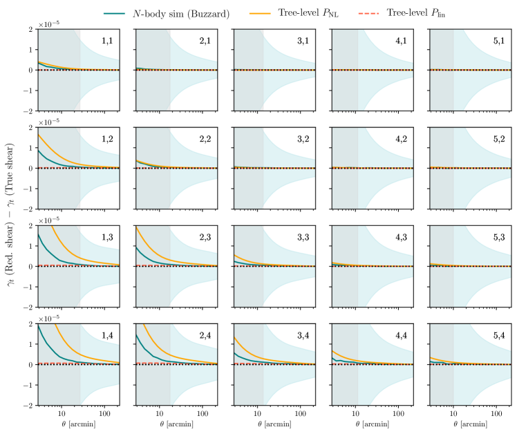
Figure 9: Reduced shear impact on the tangential shear quantity for the redMaGiC sample. We compare the results from $N$-body Buzzard simulations to the ones using theoretical predictions from CosmoLike both with Tree-level non-linear power spectrum, labeled as $P_{\rm{NL}}$, and with linear theory, labelled as $P_{\rm{lin}}$. See Krause et al. (2021) for the theoretical expressions used for these predictions. The vertical gray shading corresponds to the 6 Mpc/$h$ scale cuts and the blue shading to the tangential shear uncertainties. The numbers in each panel correspond to the lens and source redshift bins, in that order.

When a galaxy is weakly lensed, the change in its observed ellipticity is proportional to the reduced shear, $g$, which is related to both the shear and the convergence as:

$$g=\frac{\gamma}{1-\kappa}\simeq\gamma\,(1+\kappa),$$ (54)

using a Taylor expansion in the last step. Since $|\gamma|,|\kappa|\ll 1$ for individual galaxies in the weak lensing regime, the reduced shear is typically approximated by the shear, in what is known as the reduced shear approximation. In this work we make use of this approximation, and here we test whether that is sufficient for the current analysis, given DES Y3 uncertainties.

After performing the expansion correlating with the observed density field in Eq. (53), we have computed the reduced shear term $\left<\delta_{g}^{\text{int}}\,\gamma\,\kappa_{s}\right>$ using CosmoLike – see Eq. 42 from Krause et al. (2021) for the expression with the expanded integrals using Tree-level perturbation theory. We have also estimated the impact of the reduced shear approximation using the Buzzard $N$-body simulations, directly comparing the tangential shear measurements obtained with true shear compared with the shear contaminated with the $(1-\kappa)^{-1}$ factor. In Fig. 9 we compare the different estimates of the reduced shear effect to the tangential shear estimator, including two theoretical estimates using a tree-level bispectrum based on the non-linear power spectrum $P_{\text{nl}}$ or on the linear power spectrum $P_{\text{lin}}$. The tree-level bispectrum with $P_{\text{nl}}$ is known to not be an accurate model and the numbers obtained from that are useful as an upper limit only. The Buzzard estimate is expected to be the most accurate at large scales and intermediate scales, with the only the limiting factors being limited resolution at the smallest scales, especially for the low lens redshift bins, and some level of noise from the measurements. Still, to perform the robustness tests we use the the largest estimate of the three to be conservative. Comparing the addition of reduced shear using the theoretical estimate with the Tree-level $P_{\text{nl}}$ with the fiducial modeling, we find a $\Delta\chi^{2}=0.45$ after the scale cuts of 6 Mpc/$h$ without point mass marginalization and $\Delta\chi^{2}=0.15$ with PM marginalization. This translates to a shift of 0.07$\sigma$ in the 2D $\Omega_{m}-S_{8}$ plane (Krause et al., 2021). Within the DES Y3 3$\times$2pt analysis, we have adopted the threshold of 0.3$\sigma$ shifts in the $\Omega_{m}-S_{8}$ plane to decide whether some effect is significant enough to be included in the fiducial model. Therefore we found the reduced shear approximation to be good enough for the 3$\times$2pt DES Y3 analysis. In this work we have not computed the term that comes out of the coupling between lens magnification and reduced shear since it would be smaller than the reduced shear only term, and therefore negligible for our analysis. However, this term might become important in future analyses.

V.3.2 Source magnification and source clustering

Here we consider the effects of source magnification and source clustering, which both impact the observed source number density. Given our choice of estimator for the tangential shear signal, Eq. (18), we are sensitive to the density of source galaxies in three ways: (1) the boost factors; (2) intrinsic alignments; and (3) the relative weighting of lenses and sources in the sample given that we are averaging the tangential shear in lens-source galaxy pairs. The boost factors, which come from the excess number of lens-source pairs due to clustering, are discussed in Sec. III.2. We correct for this effect on the measurement side to match the theoretical predictions for the tangential shear signal that use the mean survey $n(z)$. The impact of intrinsic alignments is modulated by the number of observed source galaxies. Thus, any correlation between intrinsic galaxy ellipticity and observed source density can appear in the signal.

The third effect above arises because the tangential shear signal is weighted by the source positions, both their angular positions and redshifts. Lenses with more observed background sources will receive more weight in the signal. This effect can potentially bias the tangential shear signal when the source observed density is correlated with the lens density, for instance via magnification or when lenses and sources overlap in redshift. It could be partially removed if we averaged the tangential shear for each lens galaxy and then we averaged again over all lenses to ensure that they are weighted equally, modulo the lens weights themselves (e.g. Taylor et al. 2020). However, we choose to average the tangential shear in lens-source pairs because of the significant increase in S/N this method yields, due to optimal handling of shape noise.

We note that if we had access to the true scale-dependent $n(z,\theta)$, giving the relevant source number density as a function of separation from lens positions, we could accurately model the tangential shear signal, including the impact of source magnification and source clustering, and without needing any boost factor correction in the measurement since the impact of lens-source clustering on the redshift distributions would naturally be accounted for in the model. However, this information is not readily available in photometric surveys, and thus we instead test how significant these contributions are.

Source clustering refers to the clustering of source galaxies due to large scale structure. This implies we are more likely to find a galaxy for shear estimation in regions that are overdense in the underlying density field. As long as the source and the lens redshift are well-separated, the large scale structure at the source redshift is not correlated with that at lens redshift, and therefore, even if we will still be weighting the lens galaxies in front of these overdensities more, this will not bias our signal. Alternatively, if there is some correlation between the large scale structure at the redshift of the source galaxy $\delta_{s}$ and the one at lens redshift $\delta_{l}$ this can potentially bias our tangential shear estimator. To test the impact of source clustering, we use the following transformation when computing the integrals developed in Krause et al. (2021):

$$n_{\mathrm{s}}(\chi)\rightarrow n_{\mathrm{s}}(\chi)\left[1+{\delta^{(3\mathrm{D})}_{\mathrm{s}}(\hat{\mathbf{n}}\chi,\chi)}{\color[rgb]{0,0,0}}\right]\,,$$ (55)

which applies the transformation at the source redshift distribution level, with $\hat{n}$ being a line of sight unity vector.

The resulting contribution to the lensing correlations is very small, and indeed it vanishes in the Limber approximation, because sources at the lens redshift are not lensed. However, an analogous contribution exists for the source clustering-IA term, which is more important since IAs arise when lenses and sources are physically nearby, i.e. the same regime where they are clustered. We account for this in our fiducial TATT model perturbatively using the $b_{TA}$ parameter defined in Eq. (48) (also see Blazek et al. 2015).

Note that the contributions discussed here are different from the boost factor correction, which must be applied for Eq. (53) to hold – i.e. it is written assuming $\left<\delta_{g}^{\text{obs}}e^{\text{obs}}\right>$ is normalized by the “random-random” number of pairs in the tangential shear estimator since the terms are computed using the mean survey $n(z)$’s.

Source magnification refers to the magnification produced to source galaxies by the large scale structure in front of them. Because of magnification, the number density of source galaxies will be influenced by the overdensities or underdensities present at the lens redshift bin in particular. Thus, given our tangential shear estimator, lines of sight with higher matter densities will be weighted differently than those with less matter, potentially biasing the tangential shear signal. The impact depends on the characteristics of the source sample, specifically on whether the magnification factor $C_{s}$ (analog to the one defined in Eq. 51 for the lens sample) is positive or negative. For the same reason as for the source clustering case, we also model the correction at the three-dimensional $n(z)$ level. When combining both effects this leads to (Krause et al., 2021):

$$n_{\mathrm{s}}(\chi)\rightarrow n_{\mathrm{s}}(\chi)\left[1+{\delta^{(3\mathrm{D})}_{\mathrm{s}}(\hat{\mathbf{n}}\chi,\chi)}\right]\left[1+C_{\mathrm{s}}\kappa\left(\hat{\mathbf{n}},z\right)\right]\,.$$ (56)

Using CosmoLike we have computed the term that includes both reduced shear and source magnification, which has the same form as the term with only reduced shear but also including the factor $C_{s}$ that determines the strength of source magnification and is sample dependent. Analogously as for the lens sample (see Sec. IV.3) we can change the notation to: $C_{s}=2(\alpha_{s}-1)$. Elvin-Poole, MacCrann et al. (2021) has measured $\alpha_{s}$ for the DES Y3 shape catalog, using Balrog (Everett et al., 2022) and obtained the values shown in Table 1, for each of the source bins. Using these estimates for the magnification coefficients, we obtained a $\Delta\chi^{2}=1.8$ for the tangential shear part after scales cuts of >6 Mpc/$h$ without point-mass marginalization (1.3 with PM marginalization) and a corresponding shift of 0.128$\sigma$ in the 2D plane of $\Omega_{m}-S_{8}$. These estimates are based on the Tree-level bispectrum models using the non-linear power spectrum. We therefore do not find the combination of source magnification and reduced shear significant for this analysis, but it is possible this already becomes relevant for DES Y6 data. Regarding the coupling between lens magnification, source magnification and reduced shear, we have not computed this term since it will be smaller than the one we have found negligible in the current analysis.

V.4 Deflection effects

Galaxies at $z\sim 1$ are typically deflected $\sim 1$ arcmin by the large scale structure in front of them (Chang & Jain, 2014). This could in principle significantly affect our estimation of the galaxy positions, both lenses and sources, and therefore the estimated angular separation between a given lens-source pair. However, it is important to note that for source galaxies, which are the ones that will generally be experiencing more deflection, the original position does not actually matter. The only relevant position is where the light from the source galaxy is lensed by the foreground galaxy; thus we only need to consider the deflection experienced between the redshift of the lens and the observer. Lens galaxies will also be deflected. Hence, the error that will propagate into the estimation of the angular separation between a given lens-source pair comes from the difference between the deflection angles of the source and lens galaxies between the lens redshift and us. This difference, $\Delta\vec{\alpha}$, will generally be larger for larger angular separations, since the gravitational potential along more separated lines of sight will differ more. The relevant component of $\Delta\vec{\alpha}$ (the one propagating to angular separations) can be as large as $\sim 0.6$ arcmin for $z_{l}=1$ at the maximum angular separation used in this analysis, of 250 arcmin, and lower for smaller separations and lens redshift. At lens redshift $z_{l}=1$ and $\theta=10$ arcmin, the error on the spatial separation between the source and the lens is about 1%, and 0.2% for $\theta=250$ arcmin (Chang & Jain, 2014). We do not expect such errors to significantly impact the results presented in this paper nor in the DES Y3 cosmological analysis, but might need to be considered in future generation surveys.

There is a second effect to be considered. Since the relative position of a given lens-source plane will be affected by the difference in the deflection angles, this induces an error on the projection of the Cartesian ellipticity components to the tangential, as illustrated in Figure 3 of Chang & Jain (2014). This is also a second-order effect and is still below a percent (Chang & Jain, 2014). For the cross-component of the shear this becomes a first-order effect. Since we do not measure any signal in $\gamma_{\times}$ (see Sec. VI.1) we conclude this is not significantly impacting our tangential shear measurements but might become relevant in future data sets.

VI Measurement robustness tests

In the previous section we have explored the impact of several effects on our modeling of the galaxy-galaxy lensing signal. Similarly, we can assess the robustness of the galaxy-galaxy lensing measurement using DES Y3 data. In this section, we perform a series of tests that should produce a null signal when applied to true gravitational shear, but whose non-zero measurement, if significant, would be an indication of systematic errors leaking into the main galaxy-galaxy lensing observable. Other tests of the shear measurement, but not specific to galaxy-galaxy lensing, are presented in Gatti, Sheldon et al. (2021).

VI.1 Cross-component

The mean cross-component of the shear $\gamma_{\times}$, which is rotated 45 degrees with respect to the tangential shear $\gamma_{t}$, is expected to be compatible with zero if the shear is produced by gravitational lensing alone, because all the galaxy-galaxy lensing signal is captured by the tangential shear. The cross-component should also vanish in the presence of systematic effects that are invariant under parity.

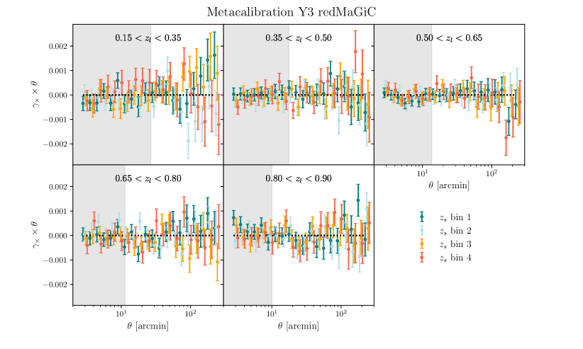
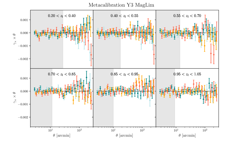
Figure 10: Cross-component of the galaxy-galaxy lensing signal around redMaGiC (top) and MagLim (bottom) lenses. The same lens-source bin combinations used for the tangential galaxy shear measurements have been considered.

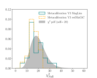
Figure 11: Null $\chi^{2}$ distribution for all the lens and source redshift bin combinations of the cross-component of the galaxy-galaxy lensing signal compared to the expected $\chi^{2}$ for 20 degrees of freedom. The blue histogram represents the MagLim lenses, while the orange histogram stands for redMaGiC lenses. In both cases the histogram is comparable to the expected $\chi^{2}$ distribution. We conclude that the $\gamma_{\times}$ measurements are compatible with a null signal.

In Fig. 10 we show the resulting cross-shear measured around MagLim and redMaGiC lenses (including random point subtraction, but not boost factors) for the exact same bin specifications used for the tangential shear. In that figure we use jackknife uncertainties (see Appendix C for a comparison of jackknife uncertainties to theoretical ones). In order to quantitatively assess the compatibility of the cross-shear with a null signal, we compute the $\chi^{2}$ of our measurements against a null signal. In Fig. 11 we present the null $\chi^{2}$ histogram coming from all the lens-source bin combinations of $\gamma_{\times}$, computed using the jackknife covariance for each lens-source bin. Note that we neglect any cross-covariance that might exist between different lens-source pairs (see Appendix A for a justification based on lognormal simulations). We consider both the MagLim and redMaGiC samples. In order to compute the $\chi^{2}=\gamma_{\times}^{T}C^{-1}\gamma_{\times}$ we need an estimate of the inverse of the covariance matrix. Given the fact that jackknife covariances contain a significant level of noise, we correct for the biased estimation of the covariance matrix with the Hartlap correcting factor, that, while not mathematically exact in the case of nonindependent realisations, it was shown by Hartlap et al. (2007) to yield accurate results also in this case. Therefore, we multiply the inverse covariance matrix by $(N_{\rm JK}-p-2)/(N_{\rm JK}-1)$, where $N_{\rm JK}$ is the number of jackknife regions (150 in our case) and $p$ the number of angular bins (20 in our case). As can be seen from the figure, our results are consistent with a null signal. Note that for this test we have used all angular scales. Therefore, our cross-shear measurements are compatible with zero at all scales, not only at the ones used for the galaxy-galaxy lensing probe in the DES Y3 3$\times$2pt cosmological analysis. However, we have also checked the results considering only the largest scales (above one degree) and obtained a very good agreement with a null signal.

VI.2 PSF residuals

The estimation of source galaxy shapes involves their modeling after being convolved with the point spread function (PSF) pattern, which depends on the atmosphere and the telescope optics and which is characterized using stars in our data sample (Gatti, Sheldon et al., 2021). Here we test the impact of PSF modeling residuals on the galaxy-galaxy lensing estimator, and their compatibility with a null signal.

In particular, we consider two kinds of PSF residuals. On the one hand, we look at PSF shape residuals which are the differences between the measured shape of the (reserved) stars and the PIFF model shape (Jarvis et al., 2021) at those same locations. On the other hand, the PSF size residuals are computed by rescaling the size of the measured PSF to match the difference in PSF size between the measurement and the model of the PSF, but keeping the PSF shape to its measured value. In Figure 12 we show the measurement mean of the tangential component of the two PSF residuals we just described around redMaGiC galaxies, including the subtraction of the same quantity around random points, in the same manner as for the tangential shear signal. For the PSF shape residuals, we obtain the following null hypothesis $\chi^{2}$ values, using a jackknife covariance, for the PSF measurements in the three bands considered ($r$, $i$, $z$): 27.1, 21.5, 14.3 (for 20 data points). Correspondingly, we find the following $\chi^{2}$ values for the PSF size residuals: 15.0, 13.5, 13.6 (for 20 data points). In summary, we find no sign of contamination from PSF residuals.

Figure 12: Measurements of PSF shape and size residuals in $r,i,z$-bands, as described in §VI.2. The measurements are found to be consistent with the null hypothesis.

VI.3 Impact of observing conditions

Included in the DES Y3 GGL fiducial setup
Contribution ($\Delta\chi^{2}$ with vs. w/o) Uncertainty ($\Delta\chi^{2}$) Uncertainty Propagated? Measurement LSS weights 3.1 (3.0 with PM) 1.3 (1.2 with PM) No Shear response 405 (125 with PM) Captured by the Mult. Shear bias Yes TreeCorr approx. $\sim 1$ 0 No Boost factors 0.1 Negligible No Model Lens magnification 20  (9.4 with PM) 7.7  (3.1 with PM) No Intrinsic alignments 46  (38 with PM) 22   (20 with PM) Yes (within TATT) Source redshifts - 20  (11 with PM) Yes (on mean) Lens redshifts - 4.8  (2.4 with PM) Yes (on mean and width) Mult. Shear bias 3.7  (1.8 with PM) 0.65  (0.54 with PM) Yes
Not included in DES Y3 GGL fiducial setup
Contribution ($\Delta\chi^{2}$ with vs. w/o) Uncertainty ($\Delta\chi^{2}$) Measurement NK shear response 0.0002 Negligible Model Non-linear galaxy bias 22  (0.42 with PM) $\sim$17  ($\sim$0.16 with PM) Baryonic effects 10  (1.7 with PM) $\sim$10 ($\sim$1.7 with PM) Reduced shear 0.45  (0.15 with PM) $\sim 0.25$ Source mag. + red. shear $\sim$1.8  ($\sim$1.3 with PM) $\sim 1$

Table 5: Summary table of the effects included in the DES Y3 3$\times$2pt fiducial measurements and model that are relevant for the galaxy-galaxy lensing probe (top) and the ones that are not included (bottom) but that we test in both this paper and the DES Y3 3$\times$2pt methodology paper in Krause et al. (2021). In the first column we show the contribution of each of these effects in either the measurement or the best-fit fiducial DES Y3 3$\times$2pt model. The contribution is estimated by computing the $\Delta\chi^{2}$ between the best-fit model and the same model removing the corresponding contribution. In the second column we show the uncertainty in each of the effects, estimated computing the $\Delta\chi^{2}$ between the best-fit model and the model with a $2\sigma$ deviation in the corresponding effect. In the third column of the upper part we indicate whether the uncertainty is propagated to the cosmological contours. In this table we consider the redMaGiC lens sample. We use the inverse of the theoretical covariance with and without the point-mass marginalization (PM) to estimate the $\Delta\chi^{2}$’s, considering only the large scales used in the cosmological analysis for the galaxy-galaxy lensing part (above 6 Mpc/$h$), which include 248 points. See Section VII for more details and discussion about future prospects.

Time-dependent observing conditions are intrinsic to photometric surveys, and they may impact the derived galaxy catalogs, for instance, introducing galaxy density variations across the survey footprint. The dependence of galaxy density on observing conditions introduces a spurious clustering signal that can have a strong impact on some of the observables used in the DES Y3 cosmological analysis, particularly on galaxy clustering.

In order to correct for such dependence, a weighting scheme has been developed in Rodríguez-Monroy et al. (2021) developed to remove the dependence of lens galaxy density on observing conditions. The scheme utilizes the maps of observing conditions such as exposure time, airmass, seeing and others, to then produce a set of weights which when applied to the galaxy population no correlations are observed between galaxy density and such observational properties. The impact of such a weighting scheme is significant for galaxy clustering measurements, as expected (Rodríguez-Monroy et al., 2021). However, since galaxy-galaxy lensing is a cross-correlation between lens and source galaxies, we expect the impact of varying observing conditions, and hence of the weighting scheme, to be less important (Prat & Sánchez et al.,, 2018). In Figure 4 we show the impact of the weighting on the galaxy-galaxy lensing measurements, and we report a $\Delta\chi^{2}=4.2$ for all the scales (corresponding to 400 data points) and a $\Delta\chi^{2}=3.1$ for scales above 6 Mpc/$h$ used directly in the cosmological analysis for the redMaGiC sample (see Table 3 for similar results of the MagLim sample).

Besides this, in Fig. 16 from Appendix C we compare the Jackknife uncertainties using 150 patches to the theoretical uncertainties using the fiducial covariance used in the 3$\times$2pt analysis from Friedrich et al. (2021). The fact they agree provides some evidence that the tangential shear measurements presented in this work do not present stronger variations across the footprint than expected.

VII Summary of measurement and modeling uncertainties

In this section we discuss the contribution of each of the components of the model and the measurement as well providing an estimate of their uncertainty. We present this in Table 5. In the top part of the table we summarize the effects which are included in our fiducial model and in the bottom the ones which are not included in the fiducial model but whose impact we have estimated. We also classify the effects depending on whether they are measurement or model components. Here we detail how we compute the uncertainty column shown in the table for each of the effects and point to the part of the paper where each effect is explained:

• LSS weights: See Sec. VI.3. We determine how the uncertainty on the LSS weights propagates to the tangential shear measurements by comparing the fiducial set of weights with an alternative version that uses a different methodology. The fiducial set of weights, validated in Rodríguez-Monroy et al. (2021), is obtained using a principal component analysis of the 107 observing conditions maps, using the first 50 identified modes as the basis (labelled as ISD-PC<50 in Rodríguez-Monroy et al. 2021). We compare the impact of using the fiducial weights to applying the ones labeled as ISD-STD34 in Rodríguez-Monroy et al. (2021), which were obtained using 34 observing conditions maps as a basis instead.

• Shear response: See Sec. III.4.2. The uncertainty on the shear response correction is determined using image simulations in MacCrann et al. (2022) and propagated to the analysis using the multiplicative bias parameters, which are marginalized over in the cosmological analysis.

• TreeCorr approximation: See Sec. III.6.

• Boost factors: See Sec. III.2.

• Lens magnification: See Sec. IV.3. We determine how the uncertainty on the lens magnification model component propagates to the tangential shear total model by comparing two different set of magnification coefficients. We compare the fiducial values which are fixed in the 3$\times$2pt analysis (displayed in Table 1 and obtained using Balrog in Elvin-Poole, MacCrann et al. (2021)) to the values obtained from the data themselves, displayed in Table 2 from Elvin-Poole, MacCrann et al. (2021).

• Intrinsic alignments (IA): See Sec. IV.4. We determine the uncertainty in the tangential shear model coming from the uncertainty in the IA model by comparing the best-fit theory curve to the one generated using different IA values, chosen from a point in the 3$\times$2pt chain that is at around $2\sigma$ from the best-fit values: $A_{1}=1.02,A_{2}=-1.22,\alpha_{1}=-0.016,\alpha_{2}=0.41,b_{TA}=0.14$ (vs $A_{1}=0.60,A_{2}=-0.16,\alpha_{1}=4.2,\alpha_{2}=3.8,b_{TA}=0.074$ for the best-fit). We do not include uncertainty coming beyond the TATT model.

• Source redshifts: We do not show the contribution of the source redshifts to the model since they are essential, i.e., the model cannot be computed without an estimated redshift distribution. We compute the uncertainty comparing the best-fit model to values in the source redshift parameters that are $2\sigma$ away from the best-fit values in the 3$\times$2pt posterior.

• Lens redshifts: Analogous to the source redshifts.

• Multiplicative shear bias: The uncertainty is computed analogously to one for redshifts.

• NK shear response: See Sec. III.4.2. This test corresponds to using the scale dependent response factors using the NK correlations within TreeCorr.

• Non-linear galaxy bias: See Sec. V.1. The contribution from higher-order terms to the fiducial linear galaxy bias model together with the baryonic effects described below was the main limitation to define scale cuts. We estimate its uncertainty by comparing the fiducial non-linear bias model used for scale cuts (and shown in Fig. 8) with the same model generated with different values for the higher-order $b_{2}$ term. The values from the $b_{2}$ term have been obtained from a point in the 3$\times$2pt chain assuming non-linear bias that is separated $\sim$2$\sigma$ from the best-fit values (specifically $0.83,1.04,-0.38,0.17,3.72$, for each of the lens redshift bins, in comparison with the original $0.38,0.37,0.44,0.72,0.90$ values).

• Baryonic effects: See Sec. V.1. To estimate the uncertainty in the baryonic effects on the galaxy-galaxy lensing probe we compare the fiducial contamination obtained from the OWLS hydrodynamic simulation (Schaye et al., 2010; van Daalen et al., 2011) to contamination from the EAGLE simulation (Schaye et al., 2015). The contamination coming from EAGLE is much smaller than the OWLS one and actually almost negligible over the scales that we use for the cosmology analysis. That is the reason why in the table the contribution and uncertainty have a similar value.

• Reduced shear: See Sec. V.3.1. We estimate the uncertainty in this higher-order effect using the differences between the theoretical model for the reduced shear labeled as Tree-level $P_{\text{NL}}$ in Fig. 9 and the one estimated from the Buzzard $N$-body simulation, also shown in that figure.

• Source magnification + Reduced shear: See Sec. V.3.2. We estimate its uncertainty scaling the uncertainty we obtain from the reduced shear effect (since the source magnification term is computed using the same base integral).

Analyzing in detail the contribution and uncertainties of the current analysis is also useful to help us make predictions for future analyses, including understanding better what the limitations will be. A critical question for larger lensing datasets, such as DES Y6, and the Euclid, LSST and WFIRST lensing surveys, is how the control of uncertainties will be improved. This improvement is required to keep them subdominant to statistical errors. While we have not studied this challenging problem here, the results summarized in Table 5 provide a basis for figuring out the prospects for galaxy-galaxy lensing. A number of sources of uncertainty are small enough that we can be confident they will remain subdominant for a survey with S/N that is 2-4 times larger (e.g. Boost factors with DES Y6 and LSST Year 1 data). Other sources of uncertainty, such as source redshifts may require improved calibration, while astrophysical effects such as intrinsic alignments may require improved theoretical modeling coupled with empirical constraints. We leave this exercise for future work.

VIII Conclusions

We obtain and validate the galaxy-galaxy lensing measurements that are used in the DES Y3 3$\times$2pt analysis (DES Collaboration, 2022). They are also used in the 2$\times$2pt analyses (Pandey et al., 2021; Porredon et al., 2021a) and to obtain the small scale lensing ratios described in Sánchez, Prat et al. (2021) that are then used in the cosmic shear analyses (Amon et al. 2022; Secco, Samuroff et al. 2022). We measure the mean tangential shear between 2.5 and 250 arcmin for two different lens galaxy samples: a sample of photometrically selected luminous red galaxies with excellent photometric redshifts (the so-called redMaGiC sample; Rozo et al. 2016; Rodríguez-Monroy et al. 2021) and a four times denser flux limited sample (MagLim; Porredon et al. 2021b), which is used as fiducial in the 3$\times$2pt analysis. For source galaxy shears we use the DES Y3 Metacalibration catalog described in Gatti, Sheldon et al. (2021). We validate the measurements both in the large-scale regime used in the cosmological analysis (above $6h^{-1}$ Mpc) and in the small scale regime (below $6h^{-1}$ Mpc) which is used for the shear-ratio analysis (Sánchez, Prat et al., 2021). The same measurement methodology and testing we develop in this paper is also used in Zacharegkas et al. (2022) to extend the measurements to smaller scales (down to 0.25 arcmin) in order to fit them with a halo occupation distribution (HOD) model. We also present and illustrate the different components of our fiducial model, which was defined in Krause et al. (2021), and discuss the impact of higher-order lensing effects.

Our fiducial mean tangential shear measurements are the highest signal-to-noise galaxy-galaxy lensing measurements to date. For the magnitude-limited sample we obtain a S/N of $\sim$148 ($\sim$120 for redMaGic). The S/N becomes $\sim$67 ($\sim$55) after applying the scale cut of 6 Mpc/$h$ and removing the two highest redshift bins for the MagLim sample, which are excluded from the DES Y3 3x2pt cosmological analysis. After applying the point-mass marginalization scheme developed in MacCrann et al. (2020) to localize the tangential shear measurements the S/N becomes $\sim$32 for MagLim and $\sim$28 for redMaGiC. Our fiducial measurements include boost factors, random point subtraction and a correction for the mean shear Metacalibration response. We find that the approximation of using the mean shear response for each source redshift bin — instead of averaging the response for lens-source pairs falling in each angular bin — is highly accurate given the current uncertainties. Therefore scale-dependent shear responses are not needed in this analysis and will likely not be necessary for future data sets either. In this analysis we use a sample of random points which is 40 times more numerous than the lens sample. We find that this adds a minor level of noise but recommend using more random points in future analysis to further minimize the impact of this effect. We find that the boost factors, which correct for lens-source clustering effects on the redshift distributions, are negligible for large scales but become relevant at small scales. We also conclude the tangential shear measurements are robust to observing conditions and PSF model residuals, as well as obtaining that the cross-component of the shear is compatible with the null.

The fiducial model used in the DES Y3 3$\times$2pt analysis is based on the non-linear matter power spectrum from Halofit (Takahashi et al., 2012) with a linear galaxy bias model validated with higher-order effects (Pandey et al., 2021), a Fourier-to-real space curved-sky projection and angular bin averaging. To account for the fact that the mean tangential shear quantity is non-local, we analytically marginalize over a point-mass following the procedure described in MacCrann et al. (2020). We also include effects from lens magnification, with the constants of proportionality determined from Balrog image simulations in Elvin-Poole, MacCrann et al. (2021), a five-parameter intrinsic alignment (IA) model that includes tidal-alignment and tidal-torquing terms (TATT) and source galaxy bias effects, and terms including the interplay between lens magnification and IA effects. We have performed an extensive code comparison of our fiducial model pipeline, CosmoSIS, with the CosmoLike code. We find this model to be a decent fit to the data with a $\chi^{2}$ of 236.3 for 192 data points for MagLim and a $\chi^{2}$ of 285.7 for 248 data points for redMaGiC, for the tangential shear part.

In this work we also explore and illustrate the impact of source magnification, source clustering and reduced shear, and how they interplay with each other and with the other effects already included in our fiducial model. We discuss how these effects depend on the chosen estimator, in this case the mean tangential shear averaged over lens-source pairs. In this work together with Krause et al. (2021) we find none of the higher-order effects or their combinations will bias our cosmological constraints by more than 0.3$\sigma$ in the $\Omega_{m}-\sigma_{8}$ plane.

Overall, we show that the high S/N tangential shear measurements presented in this work are free of systematic effects and ready to be used in the companion papers showing the combination of clustering and galaxy-galaxy lensing in Pandey et al. (2021); Porredon et al. (2021a) and the combination with cosmic shear in DES Collaboration (2022). The low statistical uncertainties of the measurements presented in this work have motivated us to perform a thorough study of several approximations that are commonly used to measure and model the mean tangential shear quantity. The impact of such effects will only become more important in the future with larger and deeper data sets. Thus, the methodology developed in this work lays the foundation for upcoming analyses, e.g. for the final DES Y6 data and future galaxy surveys such as LSST or Euclid.

Appendix A Cross-covariances in the cross-component analysis

In Sect. VI.1 we have shown that our cross-component measurements are compatible with a null signal neglecting any cross-covariance that might exist between different lens-source bin pairs. In order to support this assumption we have used lognormal simulations. This kind of simulation has shown good agreement with $N$-body simulations and real data up to nonlinear scales (Kayo et al., 2001; Hilbert, S. et al., 2011; Lahav & Suto, 2004) and have previously been used in galaxy-galaxy lensing analyses (Prat & Sánchez et al.,, 2018). We use the publicly available FLASK (Xavier et al., 2016) code to generate 1799 realizations of shear and density mock catalogs consistent with our lens and source samples. We limit ourselves to redMaGiC lenses, for simplicity, and we refer the reader to Friedrich et al. (2021) for all the details regarding the generation of the simulations. We then measure the cross-component in each one of these realizations and derive the covariance matrix. In order to be less sensitive to the exact setup used when generating the simulations and capture potential effects in the data, we combine the covariance obtained from simulations with the uncertainties obtained with the jackknife resampling. Following Sánchez et al. (2017), we normalize the simulations-derived covariance with the diagonal elements of the jackknife covariance:

$$\text{Cov}_{\theta_{i},\theta_{j}}^{\rm comb}=\text{Corr}_{\theta_{i},\theta_{j}}^{\rm FLASK}\sigma_{\theta_{i}}^{\rm JK}\sigma_{\theta_{j}}^{\rm JK}\,,$$ (57)

where Corr stands for the correlation matrix.

The full combined correlation matrix is shown in Fig. 13. We can appreciate some cross-covariance between different lens-source pairs. In more detail, we observe that pairs of lens-source bins sharing the same sources and with adjacent lenses are correlated. This is due to the same shape noise realization (of the same sources) and the overlap between adjacent lens bins that can be observed in Fig. 1. The lens-lens clustering increases the probability (above random) to have a lens in each bin near the same angular location and therefore getting the same cross-component contribution from noise.

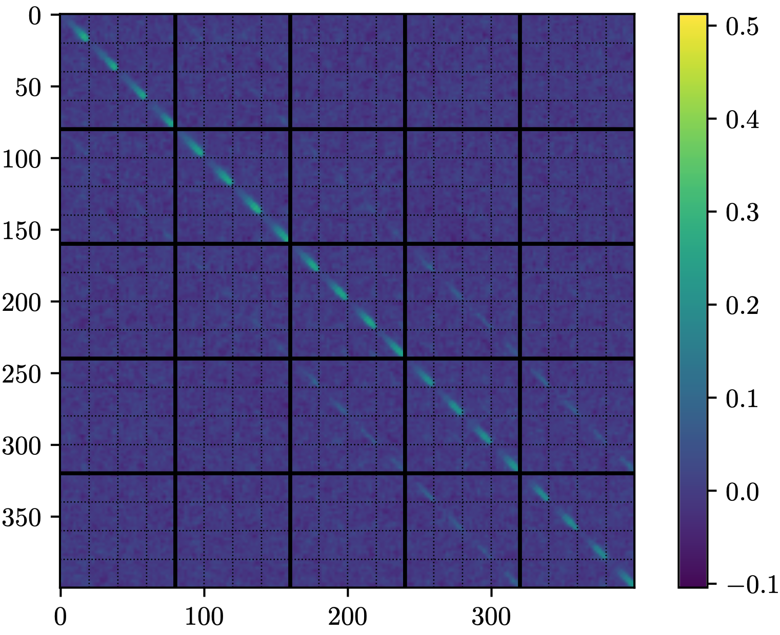
Figure 13: Correlation matrix of the cross-component for the redMaGiC sample accounting for all lens-source pairs cross-covariance using 1799 lognormal simulations combined with jackknife resampling (see the text for details). The figure shows the correlation matrix minus its diagonal for illustrative purposes. Each one of the large squares corresponds to one of the five lens bins, while the small squares correspond to one of the four source bins. Beyond the autocorrelations in each lens-source pair, we can see that bin pairs sharing the same sources and with adjacent lens bins are also correlated.

As can be seen in Fig. 13, the absolute value of these cross-covariances is much smaller than the main correlations in the diagonal $(\sim 30\%)$. However, in order to confirm whether or not the cross-covariances between different lens-source pairs can be neglected, we compute the total $\chi^{2}$ of the measured $\gamma_{\times}$ data vector with respect to a null value using this combined covariance matrix. The final value is $\chi_{\rm Null}^{2}=339$ for a data vector of 400 values. Therefore, the joint analysis also shows that our measurements of the cross-component are compatible with a vanishing signal. Note that in this case we have applied the Hartlap factor with 1799 simulations and 400 angular bins. Just for completeness, we have redone the analysis considering only the largest scales (above one degree). In this case we have obtained a final value of $\chi_{\rm Null}^{2}=117$ for a data vector of 120 values, showing that also the large-scale measurements are compatible with a vanishing signal.

Appendix B Bin-averaging and mask effects

When performing the angular bin-averaging in Eqs. (24) and (IV.1.1) we have not taken into account the variation in the pairs counts due to the survey geometry, which is expected to affect mostly large scales. This effect has been considered in previous analyses such as Asgari et al. (2019) and Singh et al. (2020c). Here we have estimated its impact computing the window auto-correlation function as

$$W(\theta)=\sum_{\ell}\frac{2\ell+1}{4\pi}P_{\ell}(\cos\theta)\,C(\ell)$$ (58)

with $C(\ell)$ being the Fourier space correlation function of the mask. The window function is shown in Fig. 14, with the value at the smallest scale normalized to unity. The variation of the window function within an angular bin provides an upper limit on the impact of this effect to the modeling of the tangential shear. We have computed the $\Delta\chi^{2}$ between the fiducial tangential shear model and the fiducial model scaled by the quantity $W(\theta_{i},\textrm{min})/W(\theta_{i},\textrm{max})$, where $i$ labels a given angular bin. We have found it has negligible impact, with a result of 0.18 using the covariance without point mass marginalization and 0.13 including the point mass, for the 248 data points considered in the cosmological analysis for the redMaGiC sample.

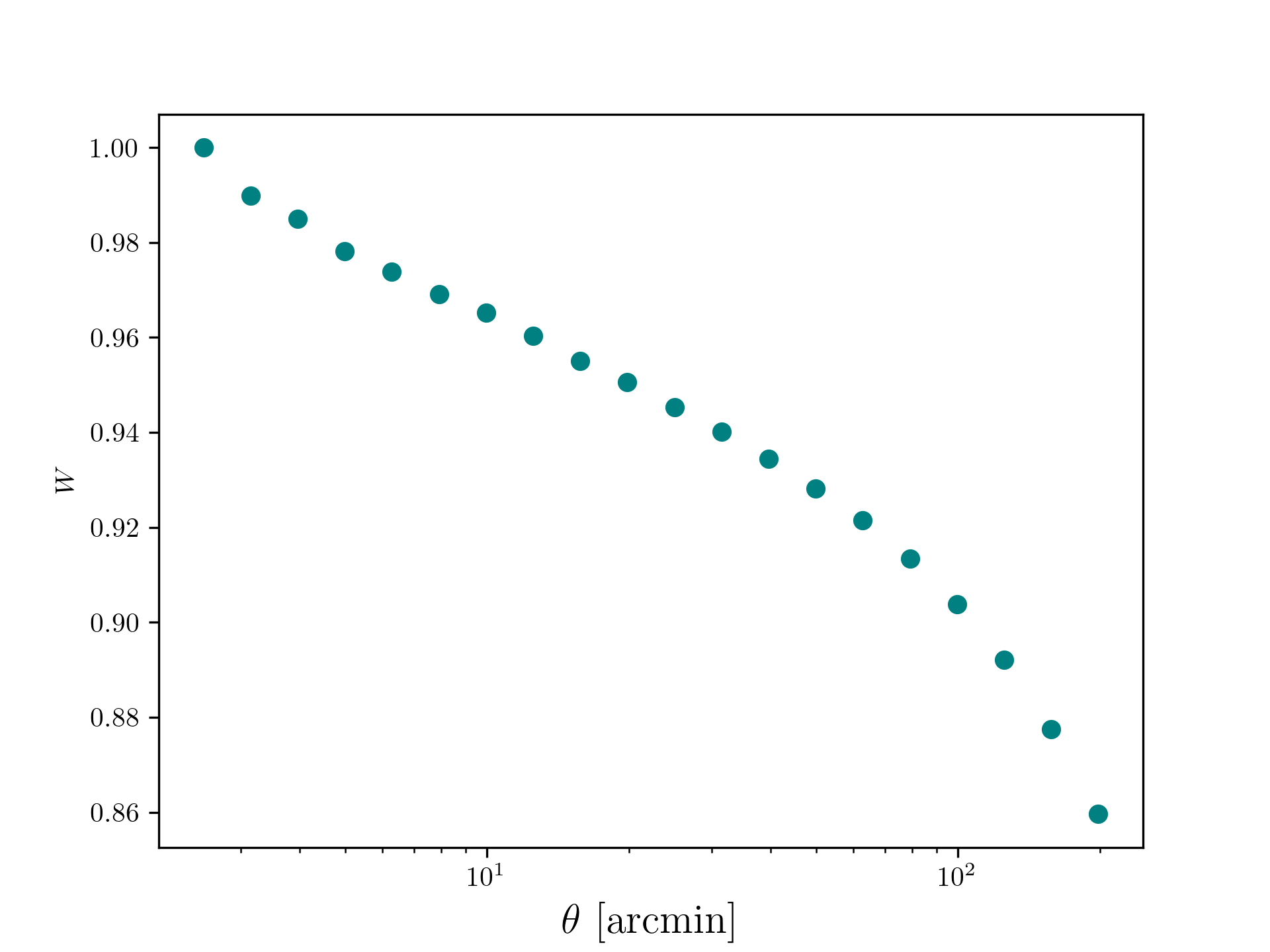
Figure 14: The survey window function $W(\theta)$ as computed from the mask auto-correlation function from Eq. (58), with the value at the smallest bin normalized to unity.

Appendix C Tangential shear around random points and Jackknife covariance tests

The mean tangential shear around random points tests the importance of geometrical and mask effects in the signal. Although our estimator of galaxy-galaxy lensing includes the subtraction of tangential shear measurement around random points, it is useful to check that this correction is small, which is shown in Fig. 15, especially for the bins with the highest signal. The uncertainties in that plot are obtained from the jackknife method, implemented as described in Sec. III.6. We compare the jackknife uncertainties (JK) to the theoretical uncertainties obtained in Friedrich et al. (2021) using a halo model covariance (Friedrich et al., 2021) in Figs. 16 and 18. We find the diagonal elements are in agreement to the 10–20% level. We also compare the uncertainties between the MagLim and the redMaGiCsamples, finding the MagLim uncertainties are significantly smaller, due to the larger number density of this sample.

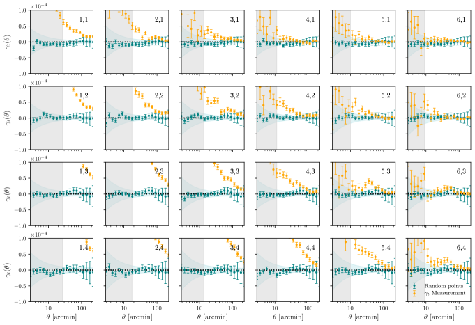
Figure 15: Tangential shear around random points using the MagLim sample as lenses in comparison with the signal, with jackknife errorbars in both cases, and comparing with the theoretical uncertainties shown in the blue bands.

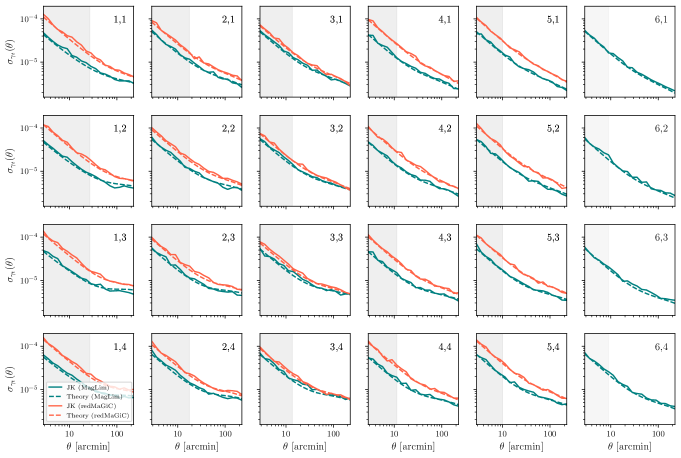
Figure 16: Comparison of the Jackknife errorbars (JK) computed in this work as described in Sec. III.6 with the theory errorbars from Friedrich et al. (2021).

Appendix D Galaxy-galaxy lensing components in Fourier space

In Fig. 17 we show the importance of each component of the model at the best-fit values of the 3$\times$2pt cosmology, analogously to Fig. 7 but now in Fourier space.

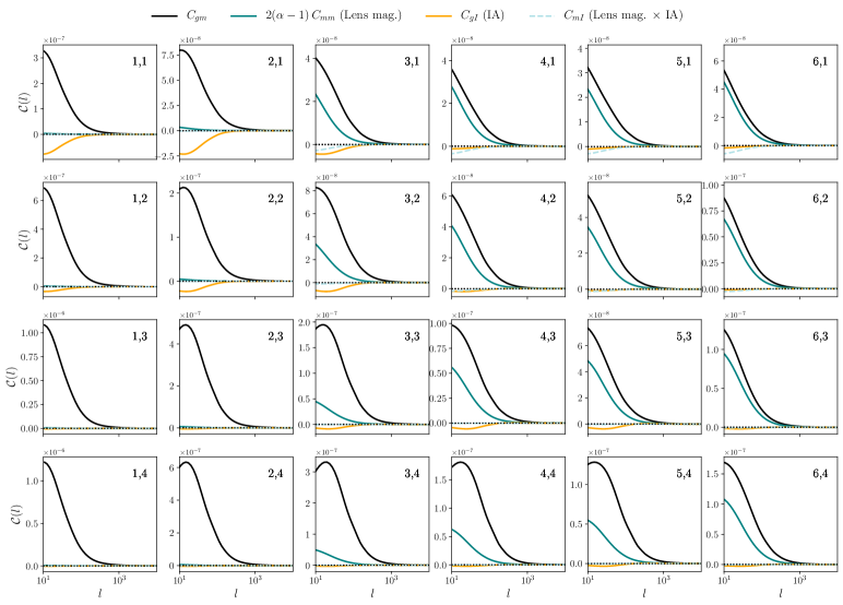
Figure 17: This plots shows the contribution from each of the components of our model in Fourier space at the best-fit values from the 3$\times$2pt results for the MagLim sample.

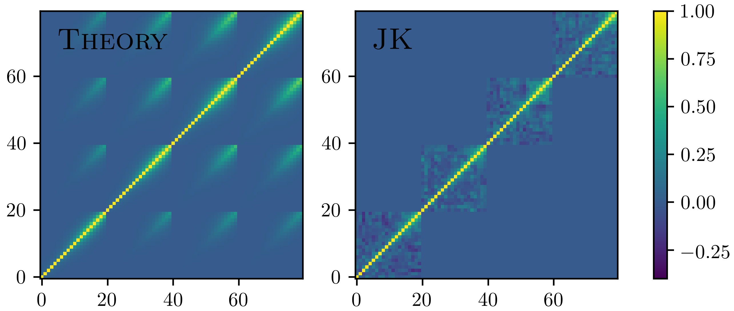
Figure 18: Correlation matrix for the redMaGiC sample using the halo-model theory covariance from Friedrich et al. (2021) (left) and the jackknife method (right). This is a subset of the covariance for the second lens bin and each of the four source redshift bins.

References

- Amon et al. (2018) Amon A., et al. 2018, MNRAS, 477, 4285
- Amon et al. (2022) Amon A., et al., 2022, Phys. Rev. D, 105, 023514
- Asgari et al. (2019) Asgari M., et al. 2019, A&A, 624, A134
- Astropy Collaboration (2018) Astropy Collaboration 2018, A.J., 156, 123
- Baldauf et al. (2010) Baldauf T., et al. 2010, Physical Review D, 81
- Baxter et al. (2016) Baxter E., et al. 2016, MNRAS, 461, 4099
- Becker (2013) Becker M. R., 2013, MNRAS, 435, 115
- Blake et al. (2020) Blake C., et al. 2020, A&A, 642, A158
- Blazek et al. (2015) Blazek J., Vlah Z., Seljak U., 2015, JCAP, 2015, 015
- Blazek et al. (2019) Blazek J. A., et al. 2019, Phys. Rev. D, 100, 103506
- Brainerd et al. (1996) Brainerd T. G., Blandford R. D., Smail I., 1996, Astrophys. J. , 466, 623
- Bridle et al. (2002) Bridle S. L., et al. 2002, Monthly Notices of the Royal Astronomical Society, 335, 1193
- Brown et al. (2002) Brown M. L., et al. 2002, Monthly Notices of the Royal Astronomical Society, 333, 501
- Burke et al. (2018) Burke D. L., et al. 2018, A.J., 155, 41
- Cawthon et al. (2020) Cawthon R., et al. 2020, arXiv e-prints, p. arXiv:2012.12826
- Chang & Jain (2014) Chang C., Jain B., 2014, MNRAS, 443, 102
- Choi et al. (2012) Choi A., et al. 2012, Astrophys. J. , 759, 101
- Clampitt et al. (2017) Clampitt J., et al. 2017, MNRAS, 465, 4204
- Cordero et al. (2022) Cordero J. P., et al. 2022, MNRAS, 511, 2170
- DES Collaboration (2016) DES Collaboration 2016, Mon. Not. R. Astron. Soc., 460, 1270
- DES Collaboration (2022) DES Collaboration 2022, Phys. Rev. D, 105, 023520
- De Vicente et al. (2016) De Vicente J., Sánchez E., Sevilla-Noarbe I., 2016, MNRAS, 459, 3078
- DeRose et al. (2019) DeRose J., et al. 2019, arXiv e-prints, p. arXiv:1901.02401
- DeRose et al. (2021a) DeRose J., Becker M. R., Wechsler R. H., 2021a, arXiv e-prints, p. arXiv:2105.12104
- DeRose et al. (2021b) DeRose J., et al., 2021b, arXiv e-prints, p. arXiv:2105.13547
- Desjacques et al. (2018) Desjacques V., Jeong D., Schmidt F., 2018, Phys. Rep., 733, 1
- Drlica-Wagner et al. (2018) Drlica-Wagner A., et al. 2018, ApJS, 235, 33
- Dvornik et al. (2019) Dvornik A., et al. 2019, Astronomy & Astrophysics, 627, A74
- Elvin-Poole et al. (2018) Elvin-Poole J., et al. 2018, Physical Review D, 98
- Elvin-Poole et al. (2021) Elvin-Poole J., MacCrann N., et al., 2021, To be submitted to MNRAS
- Everett et al. (2022) Everett S., et al., 2022, ApJS, 258, 15
- Fang et al. (2017) Fang X., et al. 2017, JCAP, 2017, 030
- Fang et al. (2020) Fang X., et al. 2020, JCAP, 2020, 010
- Flaugher et al. (2015) Flaugher B., et al., 2015, Astron. J., 150, 150
- Friedrich et al. (2021) Friedrich O., et al. 2021, MNRAS, 508, 3125
- Gatti et al. (2021) Gatti M., Sheldon E., et al., 2021, Mon. Not. Roy. Astron. Soc., 504, 4312
- Gatti et al. (2022) Gatti M., Giannini G., et al., 2022, MNRAS, 510, 1223
- Giannini et al. (2021) Giannini G., et al., 2021, Submitted to PRD
- Giblin et al. (2021) Giblin B., et al. 2021, A&A, 645, A105
- Hartlap et al. (2007) Hartlap J., Simon P., Schneider P., 2007, A&A, 464, 399
- Hartley et al. (2022) Hartley W. G., Choi A., et al., 2022, MNRAS, 509, 3547
- Heymans et al. (2021) Heymans C., et al. 2021, A&A, 646, A140
- Hilbert, S. et al. (2011) Hilbert, S. Hartlap, J. Schneider, P. 2011, A&A, 536, A85
- Hildebrandt et al. (2020) Hildebrandt H., et al. 2020, Astronomy & Astrophysics, 633, A69
- Hirata & Seljak (2004) Hirata C. M., Seljak U., 2004, Phys. Rev. D, 70, 063526
- Huff & Mandelbaum (2017) Huff E., Mandelbaum R., 2017, arXiv:1702.02600
- Jain & Taylor (2003) Jain B., Taylor A., 2003, Phys. Rev. Lett., 91, 141302
- Jarvis et al. (2004) Jarvis M., Bernstein G., Jain B., 2004, MNRAS, 352, 338
- Jarvis et al. (2021) Jarvis M., et al., 2021, Mon. Not. Roy. Astron. Soc., 501, 1282
- Joudaki et al. (2018) Joudaki S., et al. 2018, MNRAS, 474, 4894
- Kayo et al. (2001) Kayo I., Taruya A., Suto Y., 2001, The Astrophysical Journal, 561, 22
- Krause & Eifler (2017) Krause E., Eifler T., 2017, MNRAS, 470, 2100
- Krause et al. (2021) Krause E., et al. 2021, arXiv e-prints, p. arXiv:2105.13548
- Kwan et al. (2017) Kwan J., et al. 2017, MNRAS, 464, 4045
- Lahav & Suto (2004) Lahav O., Suto Y., 2004, Living Reviews in Relativity, 7, 8
- Limber (1953) Limber D. N., 1953, Astrophys. J. , 117, 134
- LoVerde & Afshordi (2008) LoVerde M., Afshordi N., 2008, Phys. Rev. D, 78, 123506
- Luo et al. (2018) Luo W., et al. 2018, The Astrophysical Journal, 862, 4
- MacCrann et al. (2020) MacCrann N., et al. 2020, MNRAS, 491, 5498
- MacCrann et al. (2022) MacCrann N., et al., 2022, MNRAS, 509, 3371
- Mandelbaum et al. (2005) Mandelbaum R., et al. 2005, MNRAS, 361, 1287
- Mandelbaum et al. (2006) Mandelbaum R., et al. 2006, MNRAS, 368, 715
- Mandelbaum et al. (2013) Mandelbaum R., et al. 2013, MNRAS, 432, 1544
- McEwen et al. (2016) McEwen J. E., et al. 2016, JCAP, 2016, 015
- Miyatake et al. (2015) Miyatake H., et al. 2015, Astrophys. J. , 806, 1
- Muir et al. (2020) Muir J., et al. 2020, MNRAS, 494, 4454
- Myles et al. (2021) Myles J., et al. 2021, MNRAS, 505, 4249
- Pandey et al. (2020) Pandey S., et al. 2020, Phys. Rev. D, 102, 123522
- Pandey et al. (2021) Pandey S., et al., 2021, arXiv e-prints, p. arXiv:2105.13545
- Park et al. (2016) Park Y., et al. 2016, Physical Review D, 94
- Park et al. (2021) Park Y., Rozo E., Krause E., 2021, Phys. Rev. Lett. , 126, 021301
- Porredon et al. (2021a) Porredon A., et al., 2021a, arXiv e-prints, p. arXiv:2105.13546
- Porredon et al. (2021b) Porredon A., et al., 2021b, Phys. Rev. D, 103, 043503
- Prat et al. (2018) Prat J., et al. 2018, Phys. Rev. D, 98, 042005
- Rodríguez-Monroy et al. (2021) Rodríguez-Monroy M., et al., 2021, Submitted to MNRAS
- Rozo et al. (2016) Rozo E., et al., 2016, Mon. Not. R. Astron. Soc., 461, 1431
- Rykoff et al. (2014) Rykoff E. S., et al. 2014, Astrophys. J., 785, 104
- Rykoff et al. (2016) Rykoff E. S., et al., 2016, Astrophys. J. Suppl. Ser., 224, 1
- Samuroff et al. (2019) Samuroff S., et al. 2019, Monthly Notices of the Royal Astronomical Society, 489, 5453
- Sánchez et al. (2017) Sánchez C., et al. 2017, MNRAS, 465, 746
- Sánchez et al. (2021) Sánchez C., Prat J., et al., 2021, Accepted by PRD
- Schaye et al. (2010) Schaye J., et al. 2010, Monthly Notices of the Royal Astronomical Society, 402, 1536
- Schaye et al. (2015) Schaye J., et al. 2015, MNRAS, 446, 521
- Schlegel et al. (1998) Schlegel D. J., Finkbeiner D. P., Davis M., 1998, Astrophys. J. , 500, 525
- Secco et al. (2022) Secco L. F., Samuroff S., et al., 2022, Phys. Rev. D, 105, 023515
- Seitz & Schneider (1997) Seitz C., Schneider P., 1997, A&A, 318, 687
- Sevilla-Noarbe et al. (2021) Sevilla-Noarbe I., et al., 2021, ApJS, 254, 24
- Sheldon & Huff (2017) Sheldon E. S., Huff E. M., 2017, Astrophys. J. , 841, 24
- Sheldon et al. (2004) Sheldon E. S., et al. 2004, A.J., 127, 2544
- Singh et al. (2017) Singh S., et al. 2017, MNRAS, 471, 3827
- Singh et al. (2020a) Singh S., et al. 2020a, MNRAS, 491, 51
- Singh et al. (2020b) Singh S., et al. 2020b, MNRAS, 491, 51
- Singh et al. (2020c) Singh S., et al. 2020c, MNRAS, 491, 51
- Takahashi et al. (2012) Takahashi R., et al. 2012, The Astrophysical Journal, 761, 152
- Taylor et al. (2020) Taylor E. N., et al. 2020, MNRAS, 499, 2896
- Unruh et al. (2020) Unruh S., et al. 2020, A&A, 638, A96
- Wechsler et al. (2021) Wechsler R. H., et al. 2021, arXiv e-prints, p. arXiv:2105.12105
- Wibking et al. (2020) Wibking B. D., et al. 2020, MNRAS, 492, 2872
- Xavier et al. (2016) Xavier H. S., Abdalla F. B., Joachimi B., 2016, Monthly Notices of the Royal Astronomical Society, 459, 3693
- Yoo & Seljak (2012) Yoo J., Seljak U., 2012, Physical Review D, 86
- Zacharegkas et al. (2022) Zacharegkas G., et al. 2022, MNRAS, 509, 3119
- Zuntz et al. (2015) Zuntz J., et al. 2015, Astronomy and Computing, 12, 45
- van Daalen et al. (2011) van Daalen M. P., et al. 2011, MNRAS, 415, 3649
- van Uitert et al. (2018) van Uitert E., et al. 2018, MNRAS, 476, 4662