Training With Data Dependent Dynamic
Learning Rates

Abstract

Recently many first and second order variants of SGD have been proposed to facilitate training of Deep Neural Networks (DNNs). A common limitation of these works stem from the fact that they use the same learning rate across all instances present in the dataset. This setting is widely adopted under the assumption that loss-functions for each instance are similar in nature, and hence, a common learning rate can be used. In this work, we relax this assumption and propose an optimization framework which accounts for difference in loss function characteristics across instances. More specifically, our optimizer learns a dynamic learning rate for each instance present in the dataset. Learning a dynamic learning rate for each instance allows our optimization framework to focus on different modes of training data during optimization. When applied to an image classification task, across different CNN architectures, learning dynamic learning rates leads to consistent gains over standard optimizers. When applied to a dataset containing corrupt instances, our framework reduces the learning rates on noisy instances, and improves over the state-of-the-art. Finally, we show that our optimization framework can be used for personalization of a machine learning model towards a known targeted data distribution.

1 Introduction

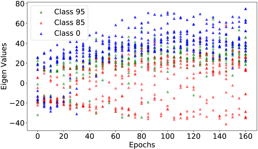
Figure 1: Eigen-value spectrum of Hessian for ResNet-18 trained on CIFAR100. For three classes, we plot top-10 eigen-values over the course of training. The loss function characteristics are different for each class.

Owing to the non-convex nature of most loss functions, coupled with poorly understood learning dynamics, optimization of Deep Neural Networks (DNNs) is a challenging task. Recent work can be broadly divided in two categories: (1) adaptive first order variants of SGD, such as ADAMw [24], RMSprop [12] and Adam [20], and (2) second order methods such as K-FAC [26]. These methods adapt the optimization process per parameter and obtain improved convergence and generalization. The objective function for these frameworks is to minimize finite-sum problems: $\mathcal{L}(\theta)=\frac{1}{N}\sum_{i}^{N}L^{i}(\theta)$, where $L^{i}(\theta)$ denotes the loss on a single training data point. Standard optimization frameworks assume that the $N$ loss functions come from the same distribution, and share characteristics such as the curvature, Lipshitz constant, etc. However, in practice, this is not true. Figure 1 highlights the difference in loss function characteristics over the course of training for classes present in CIFAR100.

In contrast to prior work, which models the learning dynamics of sum of finite problems, in this work, we account for differences in characteristics of underlying loss functions in the sum. More specifically, for each instance in the dataset, we associate a dynamic learning rate, and learn it along with model parameters. The SGD update rule for our framework takes the following form:

$$\theta^{t+1}=\theta^{t}-\frac{\lambda}{N}\sum_{i}^{N}(\mathbf{w}^{i,t}_{inst}\cdot\frac{\partial L^{i}}{\partial\theta^{t}})$$

where $L^{i}$, $\lambda$, $\mathbf{w}^{i,t}_{inst}$ denotes loss, model parameter learning rate, and multiplicative learning rate correction for instance $i$ at time step $t$. Having a dynamic learning rate per instance allows our optimization framework to focus on different modes of data during the course of optimization. Instead of using a heuristic, we learn the learning rate for each instance via meta-learning using a held out meta set. We also extend our framework to learn a dynamic learning rate per class.

The main contributions of our work are:

1. We present an optimization framework which learns an adaptive learning rate per instance in the dataset to account for differences in the loss function characteristics across instances. We extend this framework to learn adaptive learning rates per class. We also show that learning dynamic weight-decay facilitates learning dynamic learning rates on data.

2. We show that learning adaptive learning rate on data leads to variance reduction, and explains faster convergence and improved accuracy.

3. We show that in presence of noisy data, our framework reduces the learning rates on noisy instances, and prioritizes learning from clean instances. Doing so, we our method outperforms state-of-the-art by a significant margin.

4. We show that our framework can be used for personalization of machine learning models towards a targeted distribution.

2 Learning the learning rate for data

As mentioned earlier, the main goal of our work is to learn a dynamic learning rate for instances present in the train dataset. In this section, we first formalize this intution and present the framework for learning instance level learning rates. Next, we will show how our framework can be extended to learn class level learning rates. We derive our method using stochastic gradient descent (SGD) as the optimizer for model paramters, however, extension to other class of optimizers can be done in a similar manner.

2.1 Learning instance level learning rate

Let $\left\{\left(\mathbf{x}^{i}_{train},y^{i}_{train}\right)\right\}^{N}_{i=1}$ denote train set, where $\mathbf{x}^{i}\in\mathbb{R}^{d}$ denotes a single data point in the train set and $y^{i}\in\{1,...,k\}$ denotes the corresponding target. Let $f(\mathbf{x},\theta^{t})$ and $\theta^{t}$ denote the model and model’s parameters at step $t$ respectively. Let $L(\mathbf{x}^{i}_{train},y^{i}_{train};\theta^{t})$ denote an arbitrary differentiable loss function on data point $i$ at time step $t$. In what follows, we denote $L(\mathbf{x}^{i}_{train},y^{i}_{train};\theta^{t})$ as $L_{train}^{i}(\theta^{t})$. Let $\mathbf{w}_{inst}^{t}\in\mathbb{R}^{N}$ denote the instance level parameters at time step $t$. Instance level parameters weigh contribution of instances in the gradient update (see Equation 1), and can be interpreted as a multiplicative learning rate correction over the learning rate of model parameter’s optimizer. Note, learning the learning rate for each instance is equivalent to learning weighting for each instance. For the ease of explanation, we choose the latter formulation. Our goal in optimization is to solve for optimal $\hat{\theta}$ by minimizing the weighted loss on the train set:

$$\mathcal{L}_{train}(\theta^{t},\mathbf{w}_{inst}^{t}) =\frac{1}{N}\sum_{i=1}^{N}w^{i,t}_{inst}\cdot L_{train}^{i}(\theta^{t})$$ (1)

$$\hat{\theta}(\mathbf{w}_{inst}^{t}) =\arg\min_{\theta}\mathcal{L}_{train}(\theta,\mathbf{w}_{inst}^{t})$$ (2)

The solution to above equation is a function of $\mathbf{w}_{inst}^{t}$, which is not known a priori. Setting $\mathbf{w}_{inst}^{t}$ as $\mathbf{1}$ at all time steps recovers the standard gradient descent optimization framework, but that might not be optimal. This brings us to the question: What is the optimal value of $\mathbf{w}^{t}_{inst}$ i.e. the learning rate for data points at time step $t$?

Learning dynamic instance level learning rate via meta-learning

In contrast to model parameters, whose optimal value is approximated by minimizing the loss on train set, we can not approximate the optimal value of $\mathbf{w}^{t}_{inst}$ by minimizing the loss on train set. Doing so, leads to a degenerate solution, where $\mathbf{w}_{inst}^{t}=\mathbf{0}$. In principle, the optimal value of $\mathbf{w}^{t}_{inst}$ is the one, which when used to compute the gradient update at time step $t$, minimizes the error on a held-out set (referred as meta set) at convergence, i.e $\hat{\mathbf{w}}_{inst}^{t}=\arg\min_{\mathbf{w}_{inst}^{t}}\mathcal{L}_{meta}(\hat{\theta}(\mathbf{w}_{inst}^{t}))$. Here $\hat{\theta}$ denotes model parameters at convergence. The sequence of model updates from time step $t$ till convergence ($\theta^{t}\rightarrow\hat{\theta}$) can be written as a feed forward computational graph, allowing us to backpropagate meta-gradient (gradient on meta set) to $\mathbf{w}^{t}_{inst}$. However, this is not feasible in practice due to: (1) heavy compute for backpropagating through time steps, (2) heavy memory foot-print from saving all intermediate representations and (3) vanishing gradient due to backpropagation through time steps.

To alleviate this issue, we approximate the meta-gradient at convergence with the meta-gradient at time step $t+1$. More formally, we sample a mini-batch from train set, and write one step SGD update on model parameters (${\theta^{t+1}}$) as a function of instance parameters at time step $t$ (see equation 3). The one step update is used to compute loss on meta set $\mathcal{L}_{meta}({\theta^{t+1}})$, which is then used to compute the meta-gradient on instance parameters:

$${\theta^{t+1}}(\mathbf{w}_{inst}^{t}) =\theta^{t}-\frac{\lambda}{N}\sum_{i=1}^{N}\mathbf{w}^{i,t}_{inst}\frac{\partial L_{train}^{i}(\theta^{t})}{\partial\theta^{t}}$$ (3)

$$\frac{\partial\mathcal{L}_{meta}({\theta^{t+1}})}{\partial w^{i,t}_{inst}} =\frac{\partial\mathcal{L}_{meta}({\theta^{t+1}})}{\partial{\theta^{t+1}}}\cdot\frac{\partial{\theta^{t+1}}}{\partial w^{i,t}_{inst}}$$ (4)

$$\frac{\partial\mathcal{L}_{meta}({\theta^{t+1}})}{\partial w^{i,t}_{inst}} =\frac{-\lambda}{N}\cdot\frac{\partial\mathcal{L}_{meta}({\theta^{t+1}})}{\partial{\theta^{t+1}}}\cdot\big{[}{\frac{\partial L_{train}^{i}}{\partial\theta^{t}}}\big{]}^{T}$$ (5)

Here, $\lambda$ and $N$ corresponds to the learning rate of the model optimizer and number of samples in train mini-batch respectively. Using the meta-gradient on instance-parameters we update the instance-parameters using first order gradient update rule (see equation 6).

$$w^{i,t+1}_{inst} =w^{i,t}_{inst}-\lambda_{w_{inst}}\frac{\partial\mathcal{L}_{meta}({\theta^{t+1}}^{*})}{\partial w^{i,t}_{inst}}$$ (6)

The pseduo code for our method is outlined in Algorithm 1.

Algorithm 1 Learning algorithm for learning the learning rate per instance

0:  Train set $\mathcal{D}_{train}$, meta set $\mathcal{D}_{meta}$, model learning rate $\lambda$, instance parameter learning rate $\lambda_{inst}$, max iterations $T$.

0:  Model parameters at convergence $\theta^{T}$.

1:  Initialize model parameters $\theta^{0}$ and instance level parameters $\mathbf{w}_{inst}^{0}$.

2:  for $t=0$ to $T-1$ do

3:     $\{x_{train}^{i},y_{train}^{i}\}\leftarrow$ SampleMiniBatch($\mathcal{D}_{train}$).

4:     $\{x_{meta}^{j},y_{meta}^{j}\}\leftarrow$ SampleMiniBatch($\mathcal{D}_{meta}$).

5:     $\{\mathbf{w}_{inst}^{t}\}\leftarrow$ SampleInstanceParameters.

6:     Update model parameters, and express $\theta^{t+1}$ as a function of $\mathbf{w}_{inst}^{t}$ by Eq. (3).

7:     Update $\mathbf{w}_{inst}^{t+1}$ by Eq. (6).

8:  end for

Analysis of meta-gradient on instance level parameters

From equation 5, we can observe that the meta-gradient on instance parameter $\mathbf{w}_{inst}^{i,t}$ is proportional to the dot product of $i^{th}$ training sample’s gradient on model parameters at time step $t$ with meta-gradient on model parameters of samples in the meta set at time step $t+1$. Therefore, training samples whose gradient aligns with the gradients on meta-set will obtain a higher weight, leading to an increased learning rate. The converse holds true as well. For example, if an instance in train set has wrong label, its gradient will not align with gradient of clean instances in the meta set. Over the course of learning, the corrupt instance will end up obtaining a lower value of instance parameter.

2.2 Learning class level learning rate

While instance parameters have the flexibility to adapt to each instance present in the dataset, number of parameters grow with the size of dataset. To alleviate this issue, another way we can partition a dataset is by leveraging the class membership of data points. More specifically, we can learn a learning rate for each class, shared by all the instances present within the class. Let $\mathbf{w}_{class}^{t}\in\mathbb{R}^{N}$ denote the class parameters at time step $t$. Similar to equation (3), we can write the one step look ahead update as a function of class parameters, and use it compute the meta-gradient on the class parameters:

$$\frac{\partial\mathcal{L}_{meta}({\theta_{t+1}}^{*})}{\partial\mathbf{w}^{c,t}_{class}} =-\frac{\lambda.n_{c}}{N}\cdot\frac{\partial\mathcal{L}_{meta}({\theta^{t+1}}^{*})}{\partial{\theta_{t+1}}^{*}}\cdot\big{[}\frac{1}{n_{c}}{\sum\limits_{\begin{subarray}{c}i\\ y_{i}=c\end{subarray}}^{n_{c}}\frac{\partial L_{train}^{i}}{\partial\theta_{t}}}\big{]}^{T}$$ (7)

Here, $w^{c,t}_{class}$ denotes the weight for $c$ (target class for $i^{th}$ train data point), and $n_{c}$ denotes number of samples in class $c$. As seen in equation 7, the meta-gradient on class parameters is proportional to the dot-product of meta-gradient on model parameters with gradient on model parameters from train set, averaged over instances belonging to class $c$. We provide detailed derivation in supplementary material.

2.3 Meta-learning weight decay regularization

Use of weight-decay as a regularizer is a de-facto standard in training Deep Neural Networks (DNNs). However, the exact role weight-decay plays in optimization of modern DNNs is not well understood [8, 13, 24, 39]. In this section, we highlight the importance of learning the weight-decay coefficient along with the learning rate for dataset, class or instances. For ease of explanation, let us consider the case where we are interested in learning instance level learning rate, and we have the standard weight-decay term added as a regularizer.

$$\mathcal{L}_{train}(\theta^{t},w_{dataset}^{t}) =\frac{1}{N}\sum_{i=1}^{N}\mathbf{w}^{i,t}_{inst}\cdot L_{train}^{i}(\theta^{t})+\lambda_{wd}\|\theta^{t}\|$$ (8)

Here $\lambda_{wd}$ denotes the weight-decay coefficient. During the course of optimization, regardless of the magnitude of the first term, the contribution of the second term in gradient update is fixed. In our experiments, we found this to be problematic. When meta-gradient reduces the magnitude of instance parameter $\mathbf{w}^{i,t}_{inst}$, it leads to a relative increase of weight-decay component in the gradient update. This leads to destablization of the training. We solved this problem by treating the weight-decay coefficient as a learnable parameter, which is learnt along with the learning rate of class and instances using meta learning setup.

3 Experiments

3.1 Implementation details

Unless stated otherwise, the following implementation details hold true for all experiments in the paper. We use SGD optimizer (without momentum and weight-decay) to learn instance and class level learning rates. We use same batch-size to sample batches from train-set and meta-set. Apart from clamping negative learning-rates to 0, we do not employ any form of regularization, and rely on the meta-gradient to regularize the learning process. We perform $k$-fold cross validation, where the held-out set is used as both: meta-set and validation-set (for picking best configuration). For reporting final numbers, we average out dynamic learning rate trajectory for each class and instance, and use it to train on the full train-set. We ensure all methods use the same amount of training data. We report mean and standard-deviation computed over 3 runs.

3.2 Image Classification on CIFAR100

In this section, we show efficacy of our optimization framework when applied to the task of image classification on CIFAR100 [21] dataset. CIFAR100 dataset contains 100 classes, 50,000 images in the train set and 10,000 images in the test set. Therefore, in our framework, along with the model parameters, we learn 100 and 50,000 dynamic learning rates for class and instances respectively. We evaluate our framework with ResNet18 [11], VGG16 [35]. We use standard setup for training both architectures (details in supplementary).

In Figure 2, we compare our optimization framework to other optimizers commonly used in the deep learning community. Similar to results in [40], when tuned appropriately, apart from ADAM, all other optimizers obtain performance comparable to SGD. In both settings, learning class or instance level learning rate, we outperform these standard optimizers by a significant margin. These gains over standard optimizers can be attributed to the fact that our framework adapts the optimization process over samples in dataset instead of model-parameters.

Across both architectures, learning instance level learning rates performs more favorably compared to learning class level learning rates. This validates our hypothesis: loss functions for samples within a class might have different characteristics, and might benefit from learning sample specific learning rates. However, class level parameters get more frequent updates compared to instance level parameters, and hence can achieve faster convergence (see Figure 2, middle).

	ResNet18	VGG16
SGD	77.5 $\pm$ 0.0	75.4 $\pm$ 0.2
Momentum [30]	77.1 $\pm$ 0.3	74.1 $\pm$ 0.2
Adam [20]	74.4 $\pm$ 0.2	72.2 $\pm$ 0.5
AdamW [24]	77.4 $\pm$ 0.1	74.5 $\pm$ 0.2
Polyak [31]	78.0 $\pm$ 0.3	74.5 $\pm$ 0.3
LookAhead [40]	77.2 $\pm$ 0.4	75.6 $\pm$ 0.2
Instance-level	78.6 $\pm$ 0.2	76.5 $\pm$ 0.1
Class-level	78.3 $\pm$ 0.2	76.2 $\pm$ 0.2

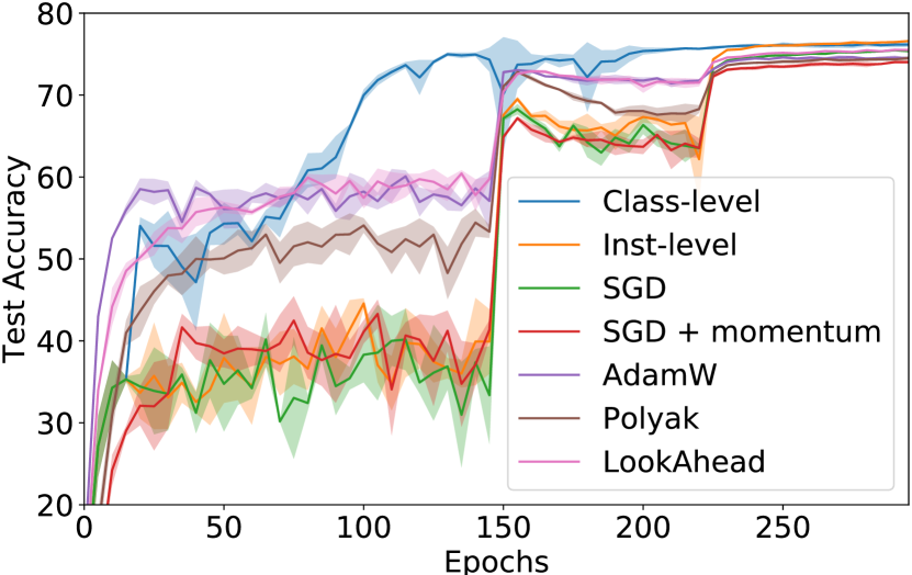
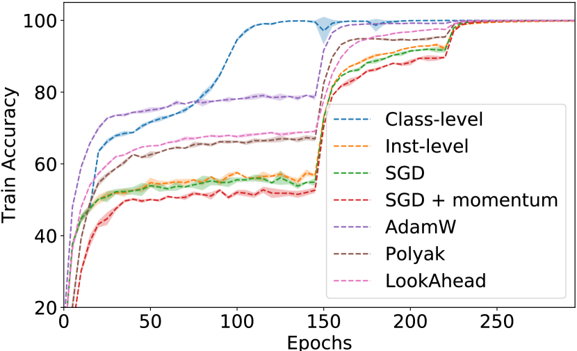
Figure 2: Table: Comparison of class and instance level optimizer with different optimizers on CIFAR100. We do a grid search on learning rate and weight-decay for other optimizers (see supplementary). Lookahead and Polyak are wrapped around SGD. Figures: Test and train accuracy for different optimizers for VGG16. Using our optimizer leads to reduced variance, and better generalization.

3.3 Analysis of optimization framework

In this section, we will analyze different components of our optimization framework.

Variance reduction via dynamic learning rates on data

One key hypothesis of our work is: loss functions for different data points can have different characteristics, and hence might benefit from different learning rates. In Figure 3 we empirically verify this property on CIFAR100, using class-level learning rates for training VGG16. In Figure 3 (A, B) we plot the train loss and test accuracy for the best (green) and the worst (red) performing class at convergence. Shared learning rate used by SGD works well for the green class, but is not able to optimize the red class (until learning rate decay at epoch 150). In contrast, our method accounts for class performance on the meta-set, and reduces the learning rate for each class in proportion to that (see Figure 3, C and D). This result provides an interesting view to our method from the perspective of variance reduction. In contrast to standard setting where methods have been proposed to reduce variance in the gradient estimator for the entire mini-batch, our work performs selective variance reduction. Lowering the learning rate for classes with worse performance will lower the overall variance in gradient estimator, leading to faster and stable convergence. In light of recent work [6], which shows ineffectiveness of standard variance reduction framework in deep learning, our results indicate that performing selective variance reduction could be an interesting direction to explore.

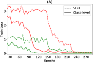
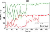
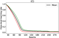
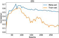
Figure 3: To speed up convergence, our framework reduces learning rate on classes with worse performance on meta set (see text for details). Learning dynamics for class with best (green) and worst (red) performance at convergence. A:Train loss. B: Test accuracy. C: Dynamic learning rate for the classes, along with mean learning rate for all classes (black). D: At each epoch, we plot the correlation of learning rate of a class with their performance on heldout meta-set and train-set.

Importance of history

	History	ResNet18	VGG16
Instance	✓	78.6 $\pm$ 0.2	76.5 $\pm$ 0.1
	✗	77.8 $\pm$ 0.2	75.4 $\pm$ 0.2
Class	✓	78.3 $\pm$ 0.2	76.2 $\pm$ 0.2
	✗	77.8 $\pm$ 0.1	75.7 $\pm$ 0.1

Table 1: Impact of retaining history on CIFAR100 for image-classification.

As mentioned earlier, learning learning rates on data points can be interpreted as learning a weighting on them. Some recent works [16, 32, 34, 38] have used meta-learning based approaches to dynamically assign weights to instances. In general, these works [16, 34, 38] train a secondary neural network to assign weights to data-points throughout the course of training, or [32] perform an online approximation of weights for each sample in the mini-batch. These frameworks are Markovian in nature, since weights estimated at each time step are independent of past predictions. In contrast, our framework treats learning rates on data as learnable parameters, and benefits from past history of optimization. In Table 1, we establish the importance of retaining optimization history, by evaluating our framework without the use of history. Specifically, after each time step, we update the model parameters using the updated value of instance and class learning rates. Post model parameter update, we reset the instance and class learning rates to their initial value of 1. As shown in Table 1, not reusing the history of learnt learning rates leads to a significant drop in performance across all settings and architectures on CIFAR100. Another place of comparison with this prior work is in noisy setting (see Section 3.4), where we outperform these methods by a significant margin.

Importance of learning a dynamic weight-decay

Recently, the importance of weight-decay in optimization of DNNs has gained much interest [8, 13, 24, 39]. [8] empirically demonstrate that weight-decay plays an important role in the first few epochs, and does not play as much a role in the later stages of training. Our results indicates otherwise. In this work, we show that learning a dynamic weight-decay leads to significant change in SGD dynamics and also facilitates the learning of learning rates on data. Figure 4 highlights the change in dynamics of SGD optimizer when weight-decay is learnt along with the model parameters. Compared to baseline (fixed weight-decay), the learnt weight-decay adapts to different stages of optimization (see Figure 4, right). More specifically, post learning rate drop, when model is most prone to overfitting, dynamic weight decay coefficient increases. This leads to a temporary drop in performance, but results in better generalization at convergence. As see in the table (Figure 4, left), learning a dynamic weight-decay improves performance of all three optimizers.

Dynamic weight decay	✗	✓
SGD	77.5 $\pm$ 0.0	78.0 $\pm$ 0.1
Class-level	77.7 $\pm$ 0.1	78.3 $\pm$ 0.2
Instance-level	78.2 $\pm$ 0.1	78.6 $\pm$ 0.2

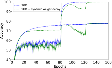
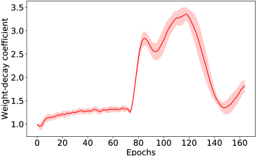
Figure 4: Evaluation of dynamic weight-decay on CIFAR100 with ResNet18. Left: Dynamic weight-decay improves all three optimizers. Center: Train (dashed) and validation (solid) accuracy for SGD optimizer, with fixed and dynamic weight-decay. Right: Plot showing the value of dynamic weight-decay when learnt along with SGD. When the learning rate drops (epoch 80, 120), weight-decay coefficient increases so as to counteract overfitting, and obtains better performance at convergence.

3.4 Results on Robust Learning

Learning instance-level learning rates can be useful when some of the labels in the dataset are noisy, where the framework should decrease learning rates on corrupt instances. In this section, we validate our framework in a controlled corrupted label setting.

To compare with the relevant state-of-the-art, we follow the common setting in ([16, 32]) to train deep CNNs, where the label of each image is independently changed to a uniform random class with probability $p$, where $p$ is noise fraction. The labels of validation data remain clean for evaluation. We compare our approach with recent state-of-the-art approaches in this setting [16, 32, 33, 34]. MentorNet [16] and Meta-Weight-Net [34] train an auxillary neural network to assign weights to samples in the mini-batch. L2RW [32] uses a held-out set to perform an online approximation of weights for samples in the mini-batch. Data parameters [33] introduced learnable temperature parameters per data-point, which scale the gradient contribution of each data point. Unfortunately, all of these works report results in two distinct settings: setting A [32] and setting B [34]. While both settings use WRN-28-10, they differ in learning rate schedules (see details in supplementary). To make a fair comparion, we report results in both settings. Similar to setup in [32, 34], we keep 1000 clean images as meta-set. As seen in Figure 5, our method outperforms other state-of-the-art methods in both settings under different levels of noise.

	40%	60%
Baseline [34]	$51.1\pm 0.4$	$30.9\pm 0.3$
Focal Loss [23]	$51.2\pm 0.5$	$27.7\pm 3.7$
Co-teaching [10]	$46.20\pm 0.15$	$35.7\pm 1.2$
Using 1000 clean images
MentorNet [16]	$61.4\pm 4.0$	$36.9\pm 1.5$
L2RW [32]	$60.8\pm 0.9$	$48.2\pm 0.3$
MWNet [34]	$67.7\pm 0.3$	$58.8\pm 0.1$
Ours (instance-level)	$\bf{69.0\pm 0.2}$	$\bf{59.6\pm 0.3}$

Setting A

	40%	80%
Baseline [32]	$50.66\pm 0.24$	$8.0$
MentorNet PD [16]	$56.9$	$14.0$
Data Parameters [33]	$\bf{70.93\pm 0.15}$	$35.8\pm 1.0$
Using 1000 clean images
MentorNet DD [16]	$67.5$	$35.0$
L2RW [32]	$61.34\pm 2.06$	-
Ours (instance-level)	$70.8\pm 0.1$	$\bf{42.5\pm 0.3}$

Setting B

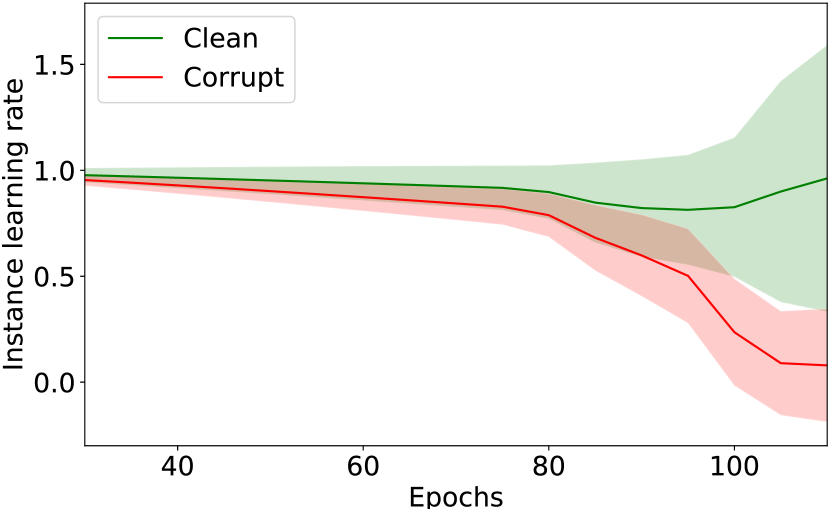
Figure 5: Tables: On CIFAR100, our methods outperforms state-of-the-art under varying levels of uniform noise in two settings (see text for details). Figure: Plot of mean and standard-deviation over instance-level learning rates for clean and corrupts instances. Our framework learns to reduce the learning rate on corrupt instances.

3.5 Personalizing DNN models

In a traditional setting, machine learning models are trained under empirical risk minimization (ERM) framework, where train and test set are assumed to be sampled from the same distribution. These models are optimized to work well across the entire data distribution. However, this training setup would not be ideal when at test time only a subset of train distribution is of interest. This situation can come up in various practical problems: (1) targeting a certain demographic for recommender systems [28], (2) personalizing models in health for a certain anomaly or demographic [14, 27], etc. In this setting, an important question one needs to answer is: What training data should I train the model on?

We simulate this scenario using the CIFAR100 dataset, which contains 100 fine grained classes, and 20 super classes (mutually disjoint, contains 5 classes). In this scenario, despite having the entire dataset annotated, we are interested in one super class at test time. Below we detail different methods which can be used in this scenario along with our proposed solution.

Biased training: The problem can be reduced to ERM framework by training the model on instances belonging to classes present in the super class. This approach makes an assumption that the other classes present in the dataset are completely disjoint from the super class. However, some of the discarded classes might share common low-level features which might be useful to train the early layers of deep neural network.

Full training: To address the aforementioned limitation, and take advantage of all the annotated data, one can train the model on all classes of the CIFAR100 dataset. However, this approach makes an assumption that training on all classes would be beneficial for the classes present in super class.

Transfer Learning: Train model on all 100 classes (full training), followed by training on the classes present in super class (biased training). A limitation of this approach is that pretraining model on all 100 classes might bias the model.

Our solution: The limitation of approaches mentioned above lies in the fact that it involves making a hard choice regarding the classes present in the training set. We relax this constraint by using dynamic class-level learning rates, which can guide the optimization process towards a biased subset dynamically. The meta set is comprised of instances belonging to the super-class.

We benchmark our method and the baselines in table below on the CIFAR100 dataset. As seen in table in Figure 6, using our proposed solution we outperform the other baselines by a significant margin.

Super Class	People	Aquatic	Vehicle 1	Electrical	Reptiles
		Mammals		Devices
Biased Training	$54.1\pm 1.3$	$69.7\pm 4.5$	$91.1\pm 0.5$	$87.0\pm 0.5$	$77.0\pm 0.5$
Full Training	$55.5\pm 1.6$	$61.1\pm 1.4$	$84.7\pm 0.5$	$77.5\pm 1.1$	$65.1\pm 1.4$
Transfer Learning	$54.6\pm 1.4$	$66.4\pm 4.1$	$91.0\pm 0.2$	$87.7\pm 0.7$	$76.2\pm 0.3$
Ours (class-level)	$\bf{61.0\pm 1.2}$	$\bf{70.7\pm 0.3}$	$\bf{93.0\pm 0.5}$	$\bf{88.1\pm 0.8}$	$\bf{79.5\pm 0.7}$

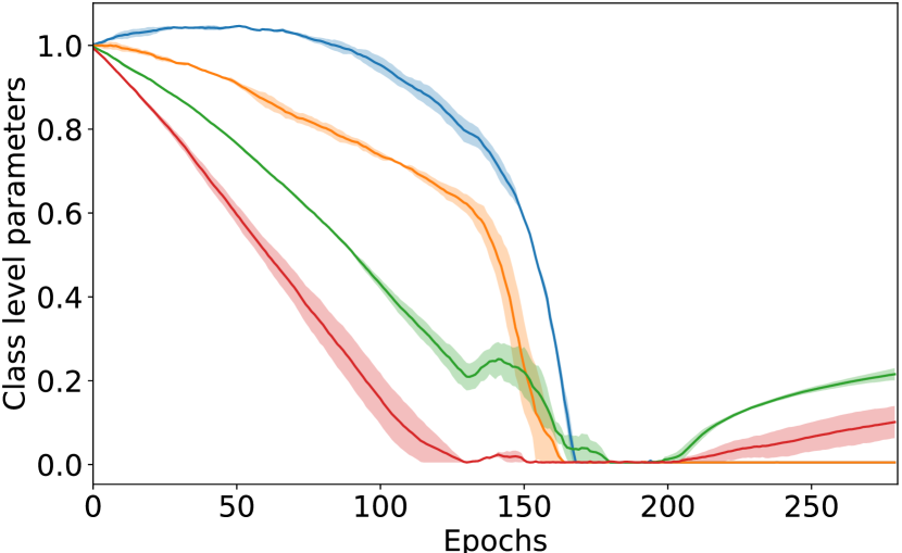
Figure 6: Table: For the task of personalization towards a super-class, using dynamic class level learning rates outperforms baselines which involve a static choice of train data. Figure: Repetable trajectories of learning rate for classes not present in the super class.

4 Related Work

Optimization of DNNs has gained a lot of interest recently [1, 13, 17, 19, 24, 26, 40] . While a full detailed review is beyond the scope of this paper, here, we give a brief overview of related work most relevant to the material present in the paper.

Learning adaptive learning rates on data can be interpreted as learning a weighting on each data point. [16, 34, 38] train an auxillary neural network to assign weights to data points. [32] performs an online approximation, where it uses one step look ahead on meta-set to estimate the weights for samples in the mini-batch. These approaches are Markovian in nature, since weights estimated at each time step are independent of past-predictions. In contrast, our method leverages the past history of optimization, and outperforms these state-of-the-art methods for robust learning (see Section 3.4).

Our work also has connections to importance sampling. [15, 17, 18] propose approximations for the gradient norm of instances which are used for sampling data points. Theoretically, sampling data points with high gradient norm should lead to faster convergence. However, this would not work well in real world dataset which contain noisy data. In the same spirit, our work also has connections to the field of curriculum learning [4, 9, 36] and self-paced learning [7, 22, 29, 37]. These approaches either design hand-crafted heuristics, or use loss value of data points as a proxy to decide the ordering of data. All these approaches require coming up with a heuristics which might not work from one problem domain to another. In contrast, our work can be interpreted as a soft differentiable form of importance sampling, where the importance of a sample (learning rate) or curriculum is learnt through meta gradient.

Data parameters [33] introduced learnable temperature parameters for each instance and class in the dataset. These parameters controlled the gradient contribution for each data point, and were learnt using gradient descent. In similar spirit, [2] introduced learnable robustness parameter per data point, which generalized different regression losses. Both of these works learn parameters per data point for robust estimation in classification or regression. In comparison, our formulation is more generic and can admit any differentiable loss function. More importantly, due to its meta-learning framework, our approach allows for robust estimation of noise as well as personalization.

Other work has proposed optimizing a few hyperparameters, such as kernel parameters [5], weight decay [3] or others [25], using gradients during training. However, to the best of our knowledge, none have done so for learning dynamic learning rates across training per se, nor done so at scale (e.g. one rate per instance) to achieve state-of-the-art performance.

5 Conclusion

In this paper, we have proposed an optimization framework which accounts for differences in loss function characteristics across instances and classes present in the dataset. More specifically, our framework learns a dynamic learning rate for each instance and class present in the dataset. Learning a dynamic learning rate allows our framework to focus on different modes of training data. For instance, when presented with noisy dataset, our framework reduces the learning rate on noisy instances, and focuses on optimizing model parameters using clean instances. When applied for the task of image-classification, across different CNN architectures, our framework outperforms standard optimizers. Finally, for the task of personalization of machine learning models towards a known data distribution, our framework outperforms strong baselines.

References

- [1] Marcin Andrychowicz, Misha Denil, Sergio Gomez, Matthew W Hoffman, David Pfau, Tom Schaul, Brendan Shillingford, and Nando De Freitas. Learning to learn by gradient descent by gradient descent. In NIPS, 2016.
- [2] Jonathan T Barron. A general and adaptive robust loss function. In CVPR, 2019.
- [3] Yoshua Bengio. Gradient-based optimization of hyperparameters. Neural computation, 2000.
- [4] Yoshua Bengio, Jérôme Louradour, Ronan Collobert, and Jason Weston. Curriculum learning. In ICML, 2009.
- [5] Olivier Chapelle, Vladimir Vapnik, Olivier Bousquet, and Sayan Mukherjee. Choosing multiple parameters for support vector machines. Machine learning, 2002.
- [6] Aaron Defazio and Léon Bottou. On the ineffectiveness of variance reduced optimization for deep learning. In NeurIPS, 2019.
- [7] Yanbo Fan, Ran He, Jian Liang, and Baogang Hu. Self-paced learning: an implicit regularization perspective. In AAAI, 2017.
- [8] Aditya Sharad Golatkar, Alessandro Achille, and Stefano Soatto. Time matters in regularizing deep networks: Weight decay and data augmentation affect early learning dynamics, matter little near convergence. In NIPS, 2019.
- [9] Guy Hacohen and Daphna Weinshall. On the power of curriculum learning in training deep networks. arXiv, 2019.
- [10] Bo Han, Quanming Yao, Xingrui Yu, Gang Niu, Miao Xu, Weihua Hu, Ivor Tsang, and Masashi Sugiyama. Co-teaching: Robust training of deep neural networks with extremely noisy labels. In NeurIPS, 2018.
- [11] Kaiming He, Xiangyu Zhang, Shaoqing Ren, and Jian Sun. Deep residual learning for image recognition. In CPVR, 2016.
- [12] Geoffrey Hinton, Nitish Srivastava, and Kevin Swersky. Neural networks for machine learning lecture 6a overview of mini-batch gradient descent.
- [13] Elad Hoffer, Ron Banner, Itay Golan, and Daniel Soudry. Norm matters: efficient and accurate normalization schemes in deep networks. In NIPS, 2018.
- [14] Natasha Jaques, Sara Taylor, Akane Sano, Rosalind Picard, et al. Predicting tomorrow’s mood, health, and stress level using personalized multitask learning and domain adaptation. In IJCAI Workshop on artificial intelligence in affective computing, 2017.
- [15] Angela H Jiang, Daniel L-K Wong, Giulio Zhou, David G Andersen, Jeffrey Dean, Gregory R Ganger, Gauri Joshi, Michael Kaminksy, Michael Kozuch, Zachary C Lipton, et al. Accelerating deep learning by focusing on the biggest losers. arXiv, 2019.
- [16] Lu Jiang, Zhengyuan Zhou, Thomas Leung, Li-Jia Li, and Li Fei-Fei. Mentornet: Learning data-driven curriculum for very deep neural networks on corrupted labels. In ICML, 2018.
- [17] Tyler B Johnson and Carlos Guestrin. Training deep models faster with robust, approximate importance sampling. In NeurIPS, 2018.
- [18] Angelos Katharopoulos and Francois Fleuret. Not all samples are created equal: Deep learning with importance sampling. In ICML, 2018.
- [19] Rahul Kidambi, Praneeth Netrapalli, Prateek Jain, and Sham Kakade. On the insufficiency of existing momentum schemes for stochastic optimization. In ICLR, 2018.
- [20] Diederik P Kingma and Jimmy Ba. Adam: A method for stochastic optimization. In ICLR, 2015.
- [21] Alex Krizhevsky. Learning multiple layers of features from tiny images. Technical report, University of Toronto, 2009.
- [22] Yong Jae Lee and Kristen Grauman. Learning the easy things first: Self-paced visual category discovery. In CVPR, 2011.
- [23] Tsung-Yi Lin, Priya Goyal, Ross Girshick, Kaiming He, and Piotr Dollár. Focal loss for dense object detection. In ICCV, 2017.
- [24] Ilya Loshchilov and Frank Hutter. Decoupled weight decay regularization. In ICLR, 2019.
- [25] Dougal Maclaurin, David Duvenaud, and Ryan Adams. Gradient-based hyperparameter optimization through reversible learning. In ICML, 2015.
- [26] James Martens and Roger Grosse. Optimizing neural networks with kronecker-factored approximate curvature. In ICML, 2015.
- [27] Kaare Mikkelsen and Maarten De Vos. Personalizing deep learning models for automatic sleep staging. arXiv, 2018.
- [28] Maxim Naumov, Dheevatsa Mudigere, Hao-Jun Michael Shi, Jianyu Huang, Narayanan Sundaraman, Jongsoo Park, Xiaodong Wang, Udit Gupta, Carole-Jean Wu, Alisson G Azzolini, et al. Deep learning recommendation model for personalization and recommendation systems. arXiv, 2019.
- [29] Te Pi, Xi Li, Zhongfei Zhang, Deyu Meng, Fei Wu, Jun Xiao, and Yueting Zhuang. Self-paced boost learning for classification. In IJCAI, 2016.
- [30] Boris T Polyak. Some methods of speeding up the convergence of iteration methods. USSR Computational Mathematics and Mathematical Physics, 1964.
- [31] Boris T Polyak and Anatoli B Juditsky. Acceleration of stochastic approximation by averaging. SIAM journal on control and optimization, 1992.
- [32] Mengye Ren, Wenyuan Zeng, Bin Yang, and Raquel Urtasun. Learning to reweight examples for robust deep learning. In ICML, 2018.
- [33] Shreyas Saxena, Oncel Tuzel, and Dennis DeCoste. Data parameters: A new family of parameters for learning a differentiable curriculum. In NeurIPS, 2019.
- [34] Jun Shu, Qi Xie, Lixuan Yi, Qian Zhao, Sanping Zhou, Zongben Xu, and Deyu Meng. Meta-weight-net: Learning an explicit mapping for sample weighting. In NeurIPS, 2019.
- [35] Karen Simonyan and Andrew Zisserman. Very deep convolutional networks for large-scale image recognition. In ICLR, 2015.
- [36] Valentin I Spitkovsky, Hiyan Alshawi, and Daniel Jurafsky. Baby steps: How “less is more” in unsupervised dependency parsing. In NIPS, 2009.
- [37] James S Supancic and Deva Ramanan. Self-paced learning for long-term tracking. In CVPR, 2013.
- [38] Xinyi Wang, Hieu Pham, Paul Michel, Antonios Anastasopoulos, Graham Neubig, and Jaime Carbonell. Optimizing data usage via differentiable rewards. arXiv, 2019.
- [39] Guodong Zhang, Chaoqi Wang, Bowen Xu, and Roger Grosse. Three mechanisms of weight decay regularization. In ICLR, 2019.
- [40] Michael Zhang, James Lucas, Jimmy Ba, and Geoffrey E Hinton. Lookahead optimizer: k steps forward, 1 step back. In NeurIPS, 2019.