Learning Model-Based Vehicle Relocation Decisions for Real-Time Ride-Sharing:
Hybridizing Learning and Optimization

Abstract

Large-scale ride-sharing systems combine real-time dispatching and routing optimization over a rolling time horizon with a model predictive control (MPC) component that relocates idle vehicles to anticipate the demand. The MPC optimization operates over a longer time horizon to compensate for the inherent myopic nature of the real-time dispatching. These longer time horizons are beneficial for the quality of relocation decisions but increase computational complexity. Consequently, the ride-sharing operators are often forced to use a relatively short time horizon. To address this computational challenge, this paper proposes a hybrid approach that combines machine learning and optimization. The machine-learning component learns the optimal solution to the MPC on the aggregated level to overcome the sparsity and high-dimensionality of the solution. The optimization component transforms the machine-learning prediction back to the original granularity through a tractable transportation model. As a consequence, the original NP-hard MPC problem is reduced to a polynomial time prediction and optimization, which allows the ride-sharing operators to consider a longer time horizon. Experimental results show that the hybrid approach achieves significantly better service quality than the MPC optimization in terms of average rider waiting time, due to its ability to model a longer horizon.

1 Introduction

Rapid growth of ride-hailing market in recent years has greatly transformed urban mobility, offering on-demand mobility services via mobile application. While major ride-hailing platforms such as Uber and Didi leverage centralized dispatching algorithms to find good matching between drivers and riders, operational challenges still persist due to imbalance between demand and supply. Consider morning rush hours as an example: most trips originate from residential areas to business districts where a large number of vehicles accumulate and remain idle. Relocating these vehicles back to the demand area is thus crucial to maintaining quality of service and income for the drivers.

There has been extensive studies on vehicle relocation problem in real-time. Previous methodologies fit broadly into two categories: optimization-based approach and learning-based approach. Optimization-based approach involves solving a mathematical program using expected demand and supply information over a future horizon to derive relocation decisions. Learning-based approach (predominantly reinforcement learning) trains a state-based decision policy from interacting with the environment and observing the rewards. While both approach have demonstrated promising performance in simulation and (in some cases) real-world deployment (Jiao et al., 2021), they have obvious drawbacks - the optimization needs to be solved in real-time and often trades off fidelity (hence quality of solutions) for computational efficiency. Reinforcement-learning approaches require a tremendous amount of data to explore high-dimensional state-action spaces and often simplify the problem to ensure efficient training. While a complex real-world problem like vehicle relocation may never admit a perfect solution, there are certainly possibilities for improvement.

This paper presents a step to overcoming these computational challenges. It proposes to replace an existing relocation optimization by a machine-learning model that predicts the optimal solutions. This makes it possible for the real-time framework to consider the optimization at higher fidelity (since the optimizations can be solved and learned offline) and therefore improve the overall quality of service. This learning step however comes with several challenges. First, the decision space is usually high-dimensional (e.g., number of vehicles to relocate between each pickup/dropoff location) and sparse, since relocations typically occur only between a few low-demand and high-demand regions. Capturing such patterns is difficult even with large amount of data. Second, the predicted solutions may not be feasible, as most predictive algorithms cannot enforce physical constraints that the solutions need to satisfy.

To solve these technical difficulties, the paper proposes an aggregation-disaggregation procedure, which learns the relocation decisions at an aggregated level to overcome the high dimensionality and sparsity of the data, and convert them back to feasible solutions at the original granularity by a transportation optimization that can be solved in polynomial time. As a consequence, in real time, the original NP-Hard optimization problem is reduced to a polynomial-time problem of prediction and optimization.

The proposed learning/optimization framework is evaluated on New York Taxi data set and achieves a $27\%$ reduction in average waiting time compared to the original relocation model due to its higher fidelity. The results suggest that a hybrid approach, that combines a high-fidelity optimization model for real-time dispatching and routing decisions and a machine-learning model for tactical relocation decisions, may provide an appealing avenue for certain classes of real-time optimizations.

The paper is organized as follows. Section 2 defines the relocation problem, Section 3 summarizes the existing literature, Section 4 reviews the relocation model, Section 5 presents the aggregation-disaggregation learning framework, and Section 6 reports the experimental results.

2 Problem Statement

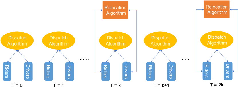
Figure 1: The real-time ride-sharing operations.

This paper considers a ride-sharing platform that uses a fixed fleet of autonomous vehicles or a pool of drivers who follow relocation instructions exactly. The platform runs a dispatching algorithm at high frequency (every 5 - 30 seconds) to match drivers with riders and a relocation algorithm at lower frequency (every 5 - 10 minutes) to relocate idle vehicles back to the demand areas (See Figure 1 for an illustration of the overall framework). Due to its forward-looking nature, the relocation optimization makes decisions based on expected demand and supply in a future time window. Longer time windows improve the quality of decision but make it harder to solve the problem in real-time. Therefore this paper learns the optimal solution of a relocation optimization with a sufficiently long horizon, and demonstrates that the learned policy achieves similar performance as the optimization model in terms of average rider waiting time and relocation costs.

3 Prior Work

Prior results on real-time idle vehicle relocation fit broadly into two frameworks: model predictive control (MPC) ((Miao et al., 2015; Zhang et al., 2016; Iglesias et al., 2017; Huang et al., 2018; Riley et al., 2020)) and reinforcement learning (RL) ((Verma et al., 2017; Oda and Joe-Wong, 2018; Guériau and Dusparic, 2018; Lin et al., 2018; Jin et al., 2019; Jiao et al., 2021; Liang et al., 2021)). MPC is an online control procedure that repeatedly solves an optimization problem over a moving time window to find the best control action. System dynamics are explicitly modeled as mathematical constraints. Due to computational complexity, all the MPC models in the literature work at discrete spatial-temporal scale (dispatch area partitioned into zones, time into epochs) and cover a relatively short time horizon.

Reinforcement learning, on the contrary, does not explicitly model system dynamics and trains a decision policy offline by approximating the state/state-action value function. It can be divided into two streams: single-agent RL (Verma et al., 2017; Oda and Joe-Wong, 2018; Guériau and Dusparic, 2018; Liang et al., 2021), and multi-agent RL (Lin et al., 2018; Jin et al., 2019; Jiao et al., 2021). Single-agent RL focuses on maximizing reward of an individual agent, and multi-agent RL maximizes collective rewards of all the agents. The main challenge of this approach is to efficiently learn the state-action value function, which is high-dimensional (often infinite-dimensional) due to the complex and fast-changing demand-supply dynamics that arises in real-time settings. Since RL relies solely on interacting with the environment to approximate the value function, a tremendous amount of samples need to be generated to fully explore the state-action space. Consequently, many works simplify the state-action space by using the same policy for agents within the same region (Verma et al., 2017; Lin et al., 2018), or restrict relocations to only neighboring regions (Oda and Joe-Wong, 2018; Guériau and Dusparic, 2018; Jin et al., 2019; Jiao et al., 2021).

Our approach tries to combine the strength of both worlds - it models the system dynamics explicitly through a sophisticated MPC model, and approximates the optimal solutions of the MPC by machine learning to overcome the real-time computational challenge. As far as the authors know, the only work that has taken a similar approach is Lei et al. (2020), where the authors propose to learn the decisions of a relocation model and show that the learned policy performs close to the original model. However, their model considers only one epoch (10 mins) and does not track how demand and supply interact over an extended period of time. This paper focuses on a much more sophisticated MPC with multiple epochs and demonstrates that the learned policy achieves superior performance than the original model due to its ability to model a longer horizon within the computational limits.

4 The Relocation Model

The underlying relocation model is an MPC model that operates over a moving time horizon. Specifically, time is discretized into epochs of equal length and, during each epoch, the MPC performs three tasks: (1) it predicts the demand and supply for the next $T$ epochs; (2) it optimizes decisions over these epochs; and (3) it implements the decisions of the first epoch. In addition, space is partitioned into zones (not necessarily of equal size or shape) and relocation decisions are made on the zone-to-zone level for each epoch. It is assumed that vehicles only pick up demand in the same zone. Once vehicles start to deliver riders or relocate, they must finish the trip before taking another assignment. These assumptions help the MPC approximates how the underlying routing/dispatch algorithm works in reality, but the dispatch algorithm does not have to obey these constraints. The only interaction between the routing/dispatch algorithm and the MPC is due to the relocation decisions. To account for waiting time, riders can only be picked up in $s$ epochs since they arrive in the system: they are assumed to drop out if waiting more than $s$ epochs.

The model formulation is presented in Figure 2. $Z$ denotes the set of zones and $\mathcal{T}=\{1,2,...,T\}$ set of time epochs in the time window. In the rest of the paper, we use $i$ and $j$ to denote zone index, and $t$ and $\rho$ to denote time index. Decision variables are as follows: $x^{p}_{ijt\rho}$ denotes number of vehicles starting to serve riders from $i$ to $j$ in $\rho$ who arrived in $t$. $x_{ijt}^{r}$ denotes the number of vehicles starting to relocate from $i$ to $j$ during $t$ ($j\neq i$), $z_{it}$ denotes the number of vehicles staying in $i$ from $t-1$ to $t$, and $l_{it}$ indicates whether there is demand unserved in zone $i$ at the end of epoch $t$.

The model inputs are the following. $D_{ijt}$ denotes number of vehicles needed to serve expected riders between $i$ and $j$ arriving at $t$. $V_{it}$ denotes number of expected idle vehicles in zone $i$ in $t$: those vehicles are busy now but will become available in $i$ in $t$. $\lambda_{ij}$ denotes number of epochs to travel from $i$ to $j$. Furthermore, $\phi(t)=\{\rho\in\mathcal{T}:t\leq\rho\leq t+s-1\}$ denotes set of valid pick-up epochs for riders arriving in epoch $t$.

Constraint (2) makes sure that vehicles do not serve more demand than there is in the allowed waiting time limit. Constraints (2) and (2) are flow balance constraints for each zone and epoch. Big-M constraints (2) and (2) prevent vehicles from relocating unless all demand in the current zone is served. The objective maximizes a weighted sum of total riders served and minimizes the total relocation cost. $W_{ij}$ is the average number of riders from $i$ to $j$ a vehicle carries: a vehicle can pick up multiple ride-sharing requests or a single request with multiple passengers, which can be estimated from historical data and taken as a parameter. $q^{p}(t,\rho)$ is the weight of a rider served at $\rho$ who arrives at $t$, and $q^{r}_{ij}(t)$ is the relocation cost between $i$ and $j$ in $t$. $q^{p}(t,\rho)$ and $q^{r}_{ij}(t)$ are decreasing in $t$ and $\rho$ since uncertainty about the future grows over time.

The model is a Mixed-Integer Linear Program (MILP), which is NP-Hard and challenging to solve at high-fidelity when the number of zones $|Z|$, or the time horizon $|\mathcal{T}|$, are large.

[2]<b> i,j∑t,ρ∑q^p(t,ρ) W_ijx^p_ijtρ - i,j∑t∑q^r_ij(t) x^r_ijt ∑_ρ∈ϕ(t) x^p_ijtρ ≤D_ijt, ∀i,j,t z_i1=0,∀i ∑_j, t_0 x^p_ijt_0 t + ∑_j x^r_ijt + z_i (t+1) = ∑_j, t_0 x^p_jit_0 (t - λ_ji) + ∑_j x^r_ji(t - λ_ji) + z_i t + V_i t,  ∀i,t ∑_j x^r_ijt≤M l_it,∀i,t ∑_j ∑_t_0:   t∈ϕ(t_0) (D_ijt - ∑_ρ=t_0^t x^p_ijt_0ρ ) ≤M(1 - l_it), ∀i,t x^p_ijtρ, x^r_ijt, z_it∈Z_+,∀i,j,t,ρ l_it∈{0,1},∀i,t

Figure 2: The MPC relocation model

5 The Learning Methodology

This section presents the overall framework for learning relocation decisions. It consists of four steps:

1. Aggregation: the decisions of the MPC model are first aggregated to the zone-level for efficient learning;

2. Learning: the aggregated decisions are learned;

3. Feasibility Restoration: the learned aggregated decisions are post-processed to restore feasibility;

4. Disaggregation: the post-processed aggregated decisions are disaggregated to the original zone-to-zone level through a transporation optimization.

Section 5.1 specifies the aggregation procedure, Section 5.2 presents the learning techniques, and Sections 5.3 and 5.4 present the method to restore feasibility and the disaggregation model.

5.1 The Aggregation Component

The overarching goal of the framework is to learn the decisions of the relocation MPC model in the first epoch, i.e., $[x^{r}_{ij1}]_{i,j\in Z}$, since these are the decisions implemented by the platform after each MPC run. In reality, the decision vector $x^{r}_{ij1}$ is often sparse, with relocation occurring only between a few low-demand zones and high-demand zones. To reduce the sparsity and the dimension of the output, $x^{r}_{ij1}$ are first aggregated to the zone level. More precisely, two metrics will be learned for each zone $i$ - the number of vehicles relocating from $i$ to other zones, i.e., $y^{o}_{i}:=\sum_{j\in Z,j\neq i}x^{r}_{ij1}$, and the number of vehicles relocating to $i$ from other zones, i.e., $y^{d}_{i}:=\sum_{j\in Z,j\neq i}x^{r}_{ji1}$. Note that these two metrics can be both non-zero at the same time - an idle vehicle might be relocated from $i$ to another zone to serve a request in the near future, and another vehicle could come to $i$ to serve a request that will arise much later. Therefore the output dimension is reduced from $|Z|^{2}$ to $2|Z|$.

5.2 The Learning Component

The learning algorithm takes essentially the same input as the MPC: the predicted supply $\mathbf{V}=[V_{it}]_{i\in Z,t\in\mathcal{T}}$ and the predicted demand $\mathbf{D}=[D_{ijt}]_{i,j\in Z,t\in\mathcal{T}}$ of idle vehicles. The aggregated relocation decisions $\mathbf{y}=[y^{d}_{i},y^{o}_{i}]_{i\in Z}$ are predicted from $\mathbf{V}$ and $\mathbf{D}$.

The trip demand in the real world often exhibits large variations. For example, business areas sees high volume of demand during weekdays and few requests on the weekend. Special events such as concerts or extreme weather could also lead to atypical demand patterns. This often causes the demand distribution and the corresponding relocation decisions to follow long-tail distribution. It is necessary to resample/reweigh the data to create a balanced data set. However, common sampling and weighting techniques are designed for univariate labels whereas $\mathbf{y}$ is a vector. One possibility is to sample the data and train a different model for each element in the label. However, this increases the training complexity and space requirements for deployment, especially when the underlying model has a large number of parameters (e.g., deep neural network). Therefore, we propose a mean-sampling and weighting heuristic to balance the data for all elements. First, the data is sampled based on the label mean: if the mean of a label falls within a predefined tail range, the observation is over-sampled. This does not guarantee, however, that the distributions of all individual elements are balanced, since each element in the label may follow a different distribution. The second step identifies elements whose distributions are still unbalanced after mean-sampling, and increases these elements’ weights in the objective function when they fall into the tail range. We experimentally demonstrate in Section 6 that this procedure learns each element accurately.

5.3 Feasibility Restoration

The feasibilty restoration turns the predictions $\mathbf{\hat{y}}=[\hat{y}^{o}_{i},\hat{y}^{d}_{i}]_{i\in Z}$ into feasible relocation decisions that are integral and obey the (hard) flow balance constraints. This is performed in three steps. First, $\hat{y}^{o}_{i}$ and $\hat{y}^{d}_{i}$ are rounded to their nearest non-negative integers. Second, to make sure that there are not more relocations than idle vehicles, the restoration sets $\hat{y}^{o}_{i}=\min\{\hat{y}^{o}_{i},V_{i1}\},\;\forall i\in Z$, where $V_{i1}$ is number of idle vehicles in zone $i$ in the first epoch. Finally, $\hat{y}^{o}_{i}$ and $\hat{y}^{d}_{i}$ need to satisfy flow balance constraint, e.g., $\sum_{i\in Z}\hat{y}^{o}_{i}=\sum_{i\in Z}\hat{y}^{d}_{i}$. This is ensured by setting the two terms to be the minimum of the two, by randomly decreasing some non-zero elements of the larger term.

$$\min\quad \sum_{i,j\in Z}c_{ij}z_{ij}$$

s.t. $$\sum_{j\in Z}z_{ij}=\hat{y}^{o}_{i},\quad \forall i\in Z$$

$$\sum_{j\in Z}z_{ji}=\hat{y}^{d}_{i},\quad \forall i\in Z$$

$$z_{ij}\in\mathbb{Z^{+}},\quad \forall i,j\in Z$$

Figure 3: The transportation problem

5.4 Disaggregation Through Optimization

The previous steps produce a feasible relocation plan $[\hat{y}^{d}_{i},\hat{y}^{o}_{i}]_{i\in Z}$ on the zone level. This last step reconstructs it to the zone-to-zone level via a transportation optimization. The model formulation is given in Figure 3. Variable $z_{ij}$ denotes the number of vehicles to relocate from $i$ to $j$, and constant $c_{ij}$ represents the corresponding relocation cost. The model minimizes the total relocation cost to consolidate the relocation plan. Its solution $z_{ij}$ will be implemented by the dispatching platform in the same way as $x^{r}_{ij1}$ was for the MPC. This optimization is a form of balanced transportation optimization problem ($\sum_{i}\hat{y}^{d}_{i}=\sum_{i}\hat{y}^{o}_{i}$): it is totally unimodular and can be solved in polynomial time by solving its linear programming relaxation. In addition, the problem is always feasible, and does not depend on the length of MPC time horizon. Therefore, the original NP-Hard MPC has been reduced to a polynomial time algorithm that transforms the predictions into a near-optimal solution to the original problem.

6 Experimental Results

The proposed learning framework is evaluated on Yellow Taxi Data in Manhattan, New York City (NYC, 2019). Several representative instances between 2015 and 2016 are selected for training, and the learned policy is tested on data during February, 2017. Section 6.1 reviews the simulation environment, Section 6.2 presents the learning results, and Section 6.3 evaluates the learned policy’s performance on the test cases.

6.1 Simulation Environment

The end-to-end ride-sharing simulator A-RTRS (illustrated in Figure 4) is used to generate data and evaluate relocation policies (Riley et al., 2020). The Manhattan area is partitioned into a grid of cells of $200$ squared meter and each cell represents a pickup/dropoff location. Travel time between the cells are queried from OpenStreetMap (2017). The fleet is fixed to be $2000$ vehicles with capacity $4$, distributed randomly among the cells at the beginning of the simulation. The simulator uses a ride-sharing routing and dispatching algorithm that batches requests into a time window and optimizes every 30 seconds (Riley et al., 2019). Its dispatching objective is to minimize a weighted sum of passenger waiting times and penalties on unserved requests. Each time a request is not served, its penalty is increased in the next batch window to ensure that the request will be scheduled with higher priority. The algorithm is solved by column generation: it iterates between solving a restricted master problem (RMP), which assigns a route to each vehicle, and a pricing subproblem, which generates feasible routes for the vehicles. The relocation MPC (Figure 2) is executed every $5$ minutes. After the MPC decides zone-to-zone level relocations, a vehicle assignment optimization determines which individual vehicles to relocate by minimizing total traveling distances. Of the three models, the dispatching model is the most computationally intensive since it operates on the individual (driver and rider) level as opposed to the zone level. Since all three models must be executed in the 30 seconds batch window, the platform allocates $20$ seconds to the dispatching optimization, $5$ seconds to the relocation optimization, and $5$ seconds to the vehicle assignment. All the models are solved using Gurobi 9.0 (Gurobi Optimization, 2020).

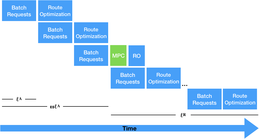
Figure 4: The A-RTRS framework

6.2 Learning Results

6.2.1 Training Data

24 taxi instances between 2015 and 2016 were selected as representative instances for learning. Each instance runs from 7 am to 9 am, with the total number of riders ranging from 19,276 to 59,820, representing a wide variety of demand scenarios in Manhattan. The instances are then perturbed by randomly adding/deleting certain percentage of requests to generate more training instances, where the percentages are sampled from a normal distribution $N(0,2.5)$. The instances are run by the simulator and the MPC results are extracted as training inputs. The MPC setup is as follows: It partitions the area into $73$ zones and time into $5$-minute epochs. The MPC time window contains $6$ epochs. Riders can be served in $3$ epochs following their arrival. Demand predictions for each O-D pair and epoch is generated by adding white noise to the true demand. The white noise is normally distributed with zero mean and a standard deviation equal to $2.5\%$ of the true demand. The number of idle vehicles in each epoch is estimated by the simulator based on current route of each vehicle and the travel times. The ride-share ratio is $W_{ij}=1.5$ for all $i,j\in Z$. Service weight and relocation penalty are $q^{p}(t,\rho)=0.5^{t}0.75^{\rho-t}$ and $q^{r}_{ij}(t)=0.001*0.5^{t}\eta_{ij}$ where $\eta_{ij}$ is travel time between zone $i$ and zone $j$ in seconds.

The MPC at such spatio-temporal fidelity is difficult to solve. With 6 cores of 2.1 GHz Intel Skylake Xeon CPU, $24.7\%$ instances could not find a feasible solution within the 5-second solver time. This was the key motivation to explore a machine-learning approach.

6.2.2 Training

The learning model is an artificial neural network with mean squared error (MSE) loss and $l_{1}$-regularization. As mentioned earlier, the data input and output often follow long-tail distribution, as highlighted in Figure 6 which shows distribution of the number of vehicles relocating to a particular zone. The mean-sampling and weighting procedure is performed in the following way: if the mean of a training label is above a certain threshold $\kappa$, the training example is duplicated $\mu$ times in the training set where $(\kappa,\mu)=(4.0,3)$ in the experiment. After the mean-sampling, some elements of the label that are zero in most training examples still exhibit a long-tail pattern. The weights of these sparse elements in the MSE loss are multiplied by a factor of $5$ on instances where they take non-zero values. This makes the training balanced for all elements.

The artificial neural network contains two fully-connected layers with hyperbolic tangent activation function and 1024 hidden units each. It is trained by the Adam optimizer in Pytorch with batch size $32$ and learning rate $10^{-3}$ (Kingma and Ba, 2014; Paszke et al., 2019). The model is trained on 10,000 data points and validated on 2000 data points. The predictions are rounded to feasible solutions by the procedure described in 5.3. Element-wise mean squared error on the validation set is reported in Table 1, and the mean absolute error of each label element as well as its mean on the validation set is given in Figure 6. The error for each element is reasonable, indicating that the model successfully learns the relocation pattern for each zone.

Table 1: The validation error before and after rounding.

Model	MSE (Pre-Rounding)	MSE (Post-Rounding)
DNN	2.01	2.05

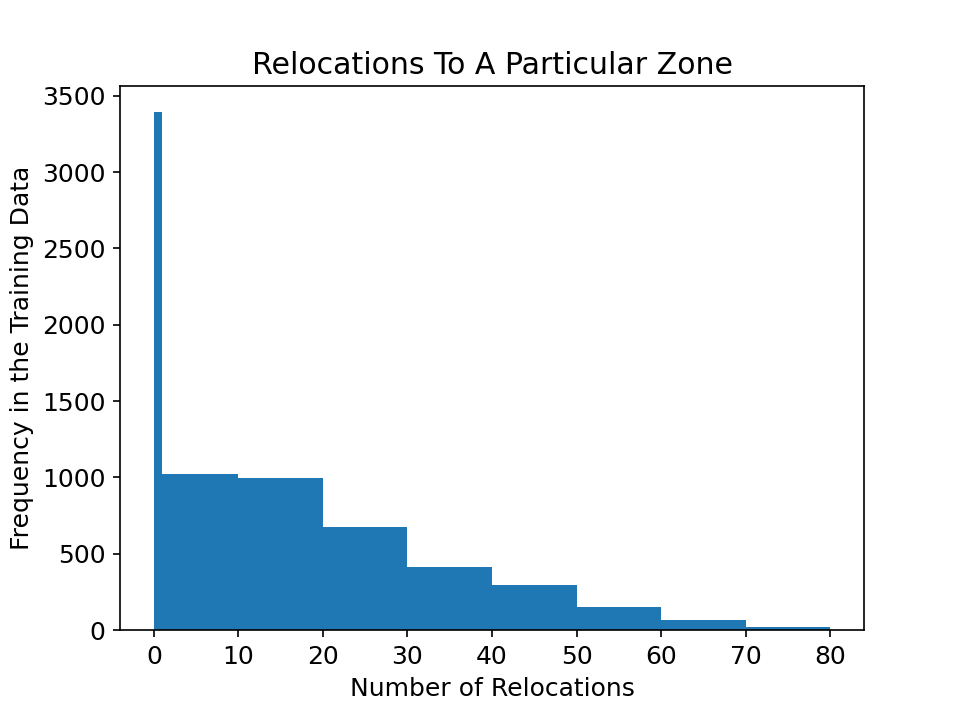
Figure 5: The distribution of relocations.

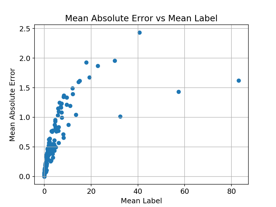
Figure 6: MAE vs mean label.

6.3 Experimental Results

The trained policy is evaluated on Yellow taxi data in February, 2017. To match with the training data distribution, days with less than $16,000$ riders between 7am and 9 am are filtered out, which leaves $22$ days. The trained policy (DNN-OPT) is compared with the original MPC model with $6$ epochs in the planning horizon (MPC-6), an MPC model with 2 epochs that represents what can be solved within the computational limit (MPC-2), and a baseline that does not perform relocations (Dispatcher). All the models use the same dispatching and routing algorithm introduced in 6.1. The rider waiting time averages, the number of relocations, and the total relocation time are reported in Figure 7. In all instances, the waiting times obtained by DNN-OPT is close to that of MPC-6, and significantly better than Dispatcher and MPC-2. The reduction in average waiting time for MPC-2, MPC-6, and DNN-OPT compared to Dispatcher are $18.7\%,47.8\%,45.6\%$ on instances with more than $25,000$ riders. This shows that DNN-OPT achieves $27\%$ further reduction in waiting time than the MPC model within the computational limit. In terms of relocations, the total number of relocations and the relocation times of DNN-OPT are also close to that of MPC-6, indicating that DNN-OPT can effectively approximate the decisions of the original model. More relocations are performed under MPC-6 and DNN-OPT than MPC-2 since longer time horizon unveils more information about the future and more opportunity for relocations. The solver times of the transportation optimization are reported in Table 2, indicating that it can be solved efficiently. The prediction time is also within fraction of a second. Overall, these promising results demonstrate that the proposed framework is capable of looking at longer time horizons for relocation, which leads to significant improvements in service quality.

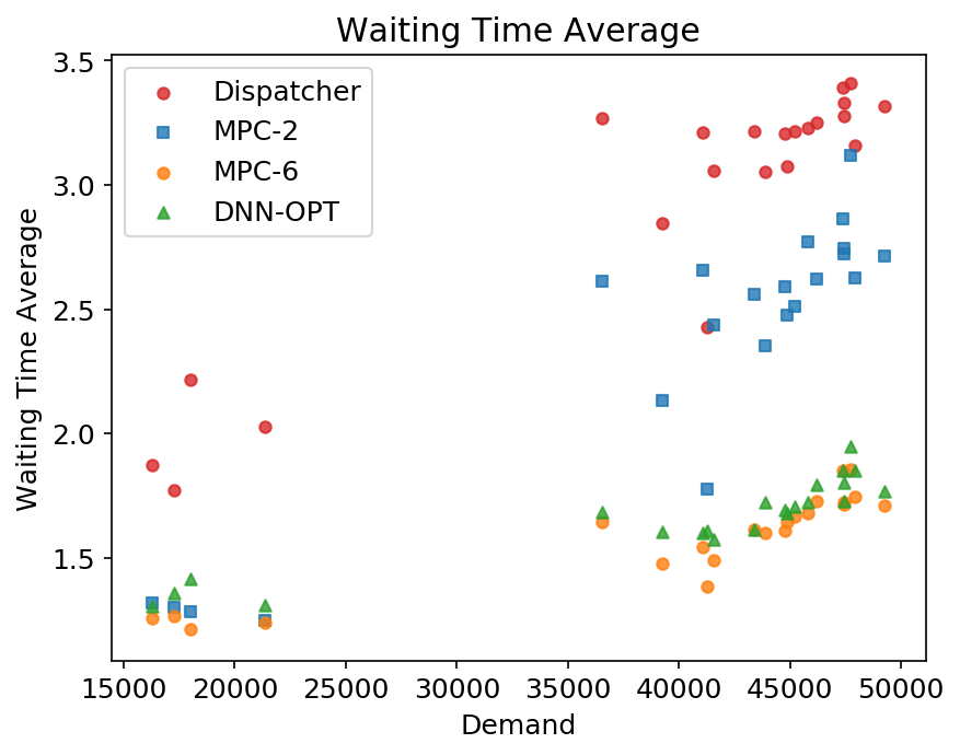
(a) Waiting time averages.

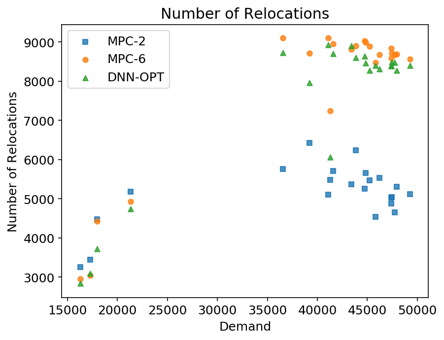
(b) Number of relocations.

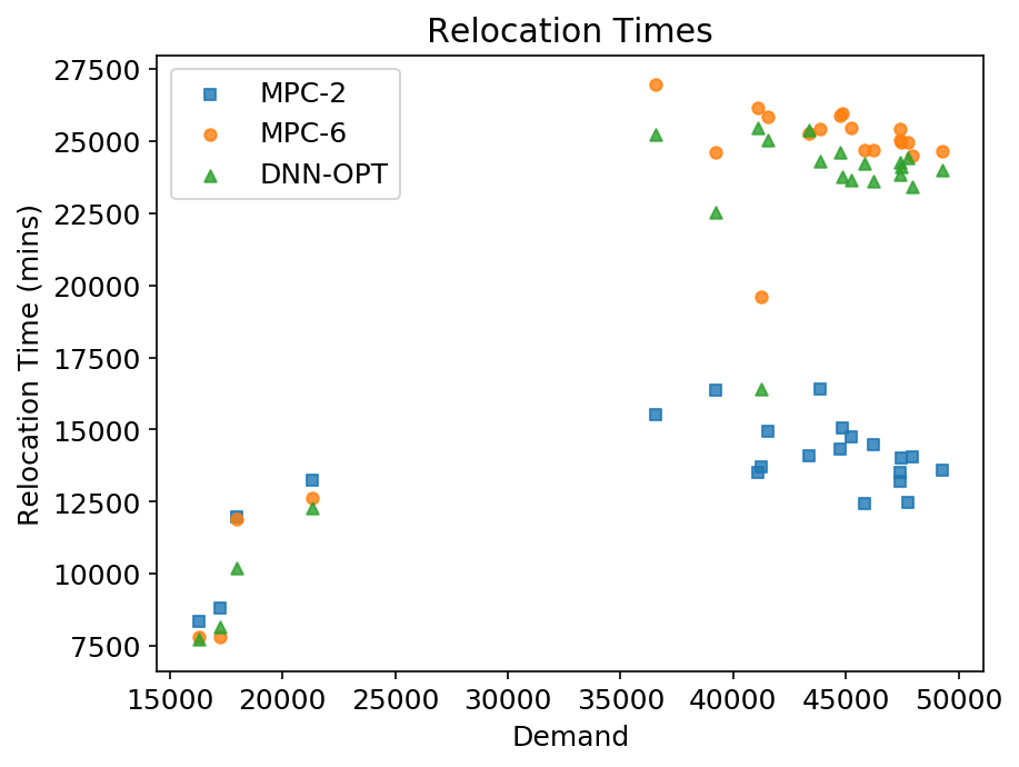
(c) Relocation times.

Figure 7: Evaluation results of DNN-OPT and its comparison with pure optimization approaches.

Table 2: The transportation model run times.

	Mean	Max
Solver Time (s)	0.02	0.05

7 Conclusion

Large-scale ride-sharing systems often combine routing/dispatching with idle vehicle relocation. The relocation optimization is based on expected demand and supply in a future time horizon. Longer time horizons improve the quality of decision but make it harder to solve the model in real-time. This paper proposes a hybrid approach combining machine learning and optimization to tackle this computational challenge. The learning component learns the optimal solution of a sophisticated relocation optimization on the aggregated (zone) level, and the optimization component transforms the prediction back to feasible solution on the zone-to-zone level via a polynomial-time transportation problem. As a consequence, the original NP-hard optimization is reduced to a polynomial time prediction and optimization, which allows the use of longer time horizons. Simulation experiments on New York Taxi data demonstrate that the learned policy achieves significantly better service quality compared to the original optimization due to its longer horizon. In particular, the proposed approach further reduces average rider waiting time by 27%. Future work is focusing on learning other important ride-sharing decisions such as dynamic pricing.

References

- Guériau and Dusparic [2018] M. Guériau and I. Dusparic. Samod: Shared autonomous mobility-on-demand using decentralized reinforcement learning. 2018 21st International Conference on Intelligent Transportation Systems (ITSC), pages 1558–1563, 2018.
- Gurobi Optimization [2020] Gurobi Optimization. Gurobi optimizer reference manual, 2020. URL http://www.gurobi.com.
- Huang et al. [2018] K. Huang, G. H. de Almeida Correia, and K. An. Solving the station-based one-way carsharing network planning problem with relocations and non-linear demand. Transportation Research Part C: Emerging Technologies, 90:1–17, 2018. ISSN 0968-090X. doi: https://doi.org/10.1016/j.trc.2018.02.020. URL https://www.sciencedirect.com/science/article/pii/S0968090X18302511.
- Iglesias et al. [2017] R. Iglesias, F. Rossi, K. Wang, D. Hallac, J. Leskovec, and M. Pavone. Data-driven model predictive control of autonomous mobility-on-demand systems. CoRR, abs/1709.07032, 2017. URL http://arxiv.org/abs/1709.07032.
- Jiao et al. [2021] Y. Jiao, X. Tang, Z. Qin, S. Li, F. Zhang, H. Zhu, and J. ping Ye. Real-world ride-hailing vehicle repositioning using deep reinforcement learning. ArXiv, abs/2103.04555, 2021.
- Jin et al. [2019] J. Jin, M. Zhou, W. Zhang, M. Li, Z. Guo, Z. Qin, Y. Jiao, X. Tang, C. Wang, J. Wang, and et al. Coride: Joint order dispatching and fleet management for multi-scale ride-hailing platforms. Proceedings of the 28th ACM International Conference on Information and Knowledge Management, Nov 2019. doi: 10.1145/3357384.3357978. URL http://dx.doi.org/10.1145/3357384.3357978.
- Kingma and Ba [2014] D. Kingma and J. Ba. Adam: A method for stochastic optimization. International Conference on Learning Representations, 12 2014.
- Lei et al. [2020] Z. Lei, X. Qian, and S. V. Ukkusuri. Efficient proactive vehicle relocation for on-demand mobility service with recurrent neural networks. Transportation Research Part C: Emerging Technologies, 117:102678, 2020. ISSN 0968-090X. doi: https://doi.org/10.1016/j.trc.2020.102678. URL https://www.sciencedirect.com/science/article/pii/S0968090X20305933.
- Liang et al. [2021] E. Liang, K. Wen, W. Lam, A. Sumalee, and R. Zhong. An integrated reinforcement learning and centralized programming approach for online taxi dispatching. IEEE Transactions on Neural Networks and Learning Systems, 02 2021. doi: 10.1109/TNNLS.2021.3060187.
- Lin et al. [2018] K. Lin, R. Zhao, Z. Xu, and J. Zhou. Efficient large-scale fleet management via multi-agent deep reinforcement learning. In Proceedings of the 24th ACM SIGKDD International Conference on Knowledge Discovery and Data Mining, KDD ’18, page 1774–1783, New York, NY, USA, 2018. Association for Computing Machinery. ISBN 9781450355520. doi: 10.1145/3219819.3219993. URL https://doi.org/10.1145/3219819.3219993.
- Miao et al. [2015] F. Miao, S. Lin, S. Munir, J. Stankovic, H. Huang, D. Zhang, T. He, and G. Pappas. Taxi dispatch with real-time sensing data in metropolitan areas — a receding horizon control approach. IEEE Transactions on Automation Science and Engineering, 13, 04 2015. doi: 10.1145/2735960.2735961.
- NYC [2019] NYC. Nyc taxi & limousine commission - trip record data, 2019. URL http://www.nyc.gov/html/tlc/html/about/trip_record_data.shtml. Accessed: 2020-10-01.
- Oda and Joe-Wong [2018] T. Oda and C. Joe-Wong. Movi: A model-free approach to dynamic fleet management. IEEE INFOCOM 2018 - IEEE Conference on Computer Communications, pages 2708–2716, 2018.
- OpenStreetMap [2017] OpenStreetMap. Planet dump retrieved from https://planet.osm.org, 2017. URL https://www.openstreetmap.org. Accessed: 2020-10-01.
- Paszke et al. [2019] A. Paszke, S. Gross, F. Massa, A. Lerer, J. Bradbury, G. Chanan, T. Killeen, Z. Lin, N. Gimelshein, L. Antiga, A. Desmaison, A. Kopf, E. Yang, Z. DeVito, M. Raison, A. Tejani, S. Chilamkurthy, B. Steiner, L. Fang, J. Bai, and S. Chintala. Pytorch: An imperative style, high-performance deep learning library. In H. Wallach, H. Larochelle, A. Beygelzimer, F. d'Alché-Buc, E. Fox, and R. Garnett, editors, Advances in Neural Information Processing Systems 32, pages 8024–8035. Curran Associates, Inc., 2019. URL http://papers.neurips.cc/paper/9015-pytorch-an-imperative-style-high-performance-deep-learning-library.pdf.
- Riley et al. [2019] C. Riley, A. Legrain, and P. Van Hentenryck. Column generation for real-time ride-sharing operations. In L.-M. Rousseau and K. Stergiou, editors, Integration of Constraint Programming, Artificial Intelligence, and Operations Research, pages 472–487. Springer International Publishing, 2019.
- Riley et al. [2020] C. Riley, P. van Hentenryck, and E. Yuan. Real-time dispatching of large-scale ride-sharing systems: Integrating optimization, machine learning, and model predictive control. In Proceedings of the Twenty-Ninth International Joint Conference on Artificial Intelligence, IJCAI-20, pages 4417–4423. International Joint Conferences on Artificial Intelligence Organization, 7 2020. doi: 10.24963/ijcai.2020/609. URL https://doi.org/10.24963/ijcai.2020/609.
- Verma et al. [2017] T. Verma, P. Varakantham, S. Kraus, and H. C. Lau. Augmenting decisions of taxi drivers through reinforcement learning for improving revenues. In ICAPS, 2017.
- Zhang et al. [2016] R. Zhang, F. Rossi, and M. Pavone. Model predictive control of autonomous mobility-on-demand systems. In 2016 IEEE International Conference on Robotics and Automation (ICRA), pages 1382–1389, 2016. doi: 10.1109/ICRA.2016.7487272.