Enhancing the performance of a bistable energy harvesting device via the cross-entropy method

Abstract

This work deals with the solution of a non-convex optimization problem to enhance the performance of an energy harvesting device, which involves a nonlinear objective function and a discontinuous constraint. This optimization problem, which seeks to find a suitable configuration of parameters that maximize the electrical power recovered by a bistable energy harvesting system, is formulated in terms of the dynamical system response and a binary classifier obtained from 0-1 test for chaos. A stochastic solution strategy that combines penalization and the cross-entropy method is proposed and numerically tested. Computational experiments are conducted to address the performance of the proposed optimization approach by comparison with a reference solution, obtained via an exhaustive search in a refined numerical mesh. The obtained results illustrate the effectiveness and robustness of the cross-entropy optimization strategy (even in the presence of noise or in moderately higher dimensions), showing that the proposed framework may be a very useful and powerful tool to solve optimization problems involving nonlinear energy harvesting dynamical systems.

1 Introduction

Energy harvesting is a process of energy conversion in which a certain amount of energy is pumped from an abundant source (e.g. the sun, wind, ocean, environmental vibrations, electromagnetic radiation, etc.) into another system that stores and/or use this energy for its self-operation Gammaitoni (2012); Priya and Inman (2009); Spies et al. (2015). This type of technology has a broad field of applicability, that includes: (i) large-scale devices such as ocean thermal energy converters Liu et al. (2019), magnetic levitators Rocha et al. (2019), etc.; (ii) middle size applications like electromechanical systems Ghouli et al. (2017); Leadenham and Erturk (2020), sensors/actuators Bhatti et al. (2016); Gallo et al. (2012); Trindade (2016), living trees Ying et al. (2015) etc.; (iii) small or very small systems, namely medical implants Pfenniger et al. (2014), micro/nano electro-mechanical systems (MEMS/NENS) Nabavi and Zhang (2016); Selvan and Ali (2016), graphene structures López-Suárez et al. (2011), bio cells Catacuzzeno et al. (2019), etc.

Enhance the amount of energy collected by an energy harvester is a key problem in the operation of these kind of devices, being the object of interest of several research works among the last decade, with efforts divided essentially in two fronts: (i) approaches with great physical appeal, which seek to explore complex geometric arrangements and nonlinearities in a smart way to improve the performance of the systemAbdelkefi et al. (2012); Benacchio et al. (2016); Daqaq et al. (2020); Dekemele et al. (2019); Harne (2012); Ibrahim et al. (2016); Ramlan et al. (2010); Vocca et al. (2012); Zhou et al. (2016); (ii) works that look at this task from a more mathematical perspective, conducting theoretical analysis in mathematical models Rechenbach et al. (2016), using control theory to optimize the underlying dynamics Barbosa et al. (2015); de la Roca et al. (2019); Sun et al. (2020); Yang and Cao (2019) or formulating and solving non-convex optimization problems to find the optimal system design Godoy and Trindade (2012); Lopes et al. (2017, 2019a); Peterson et al. (2016); Zheng et al. (2009).

The approaches that seek to optimize energy harvesters exploring their physics, in general, try to take advantage of a key (and very particular) characteristic of the dynamics, often neglected in a naive look, in favor of better performance. Although they can produce very efficient solutions for certain types of systems, they lack generality, which makes them, in a sense, an “art”, as it requires a high level of knowledge about the system behavior by the designer’s part.

On the other hand, approaches based on numerical optimization have a good level of generality, however, they come up with theoretical and computational difficulties inherent to the solution of non-convex optimization problems defined by objective functions that are constructed from observations of the nonlinear dynamical systems.

These difficulties are faced not only when dealing with energy harvesters, but they can also be seen in the optimization of several types of nonlinear dynamical systems, generally being circumvented with the use of computational intelligence-based algorithms Mangla et al. (2020); Quaranta et al. (2020), since traditional gradient-based methods have no guarantee of finding global extremes in the absence of convexity Bonnans et al. (2009); Boyd and Vandenberghe (2004); Nocedal and Wright (2006).

Among the computational intelligence algorithms available in the literature, the most frequently used for optimization in nonlinear dynamics include genetic algorithms (and their variants), particle swarm optimization, differential evolution, artificial neural networks (and other machine learning methods), etc Quaranta et al. (2020). As they are global search methods, they are often successful in overcoming the (local) difficulties faced by gradient-based methods, at the price of losing computational efficiency. But the loss of efficiency is not the only weakness of these global methods, most of then need to have the underlying control parameters tuned for proper functioning. This task is usually done manually, in a trial and error fashion, which is not at all practical, as the meaning of many of these parameters is often not intuitive. This peculiarity practically “condemns” these tools to be used in the black-box format, without much control by the user, which may induce significant losses in performance and accuracy.

However, the computational intelligence literature has at least one global search algorithm that is robust and simple, for which the control parameters are very intuitive, it is known as the cross-entropy (CE) method, proposed by R. Rubinstein in 1997 Rubinstein (1997, 1999); Rubinstein and Kroese (2004) for rare events simulation. Soon after it was realized that it could be a very appealing global search technique for challenging combinatorial and continuous optimization problems Kroese et al. (2013); Rubinstein and Kroese (2016). It is a sampling technique, from the family of Monte Carlo methods, which iteratively attacks the problem, refining the candidates to be the solution according to a certain optimality criterion.

Surprisingly, the nonlinear dynamics literature has been neglecting the CE method, although it is a relatively known technique in the combinatorial optimization community. To the best of the author’s knowledge, there are few studies in the open literature applying the CE method for numerical optimization problems involving nonlinear mechanical systems Dantas (2019); Dantas et al. (2019a, b); Ghidey (2015); Issa et al. (2018); Wang (2012), which leaves space for new contributions in this line. In particular, the development of a simplistic and robust optimization framework, easily customizable, which can be used by naive users without major performance losses.

In this context, this work deals with the numerical optimization of nonlinear energy harvesting systems, trying to find a strategy to increase the performance of a bistable energy harvesting device subjected to a periodic excitation. For this purpose, a non-convex optimization problem, with a nonlinear objective function and discontinuous constraint, is formulated and a stochastic strategy of solution that combines penalization and the CE method is proposed and numerically tested. As this method has a theoretical guarantee of convergence and evidence in the literature proving its effectiveness Kroese et al. (2013); Rubinstein and Kroese (2016), the proposed cross-entropy framework for optimization of dynamical systems has the potential to be a very general and robust numerical methodology.

The rest of this manuscript is organized as follows. Section 2 presents the energy harvesting device of interest and the underlying dynamical system. An optimization problem associated with this nonlinear system is defined in section 3, and the CE method strategy of solution is presented in section 4. Numerical experiments, conducted to test the effectiveness and robustness of the stochastic solution strategy, are shown in section 5. Finally, in section 6, final remarks are set out.

2 Nonlinear dynamical system

2.1 Physical system

The energy harvesting system of interest in this work is the (sinusoidal excited) piezo-magneto-elastic beam presented by Erturk et al. Erturk et al. (2009), which is based on the (stochastically excited) inverted pendulum energy harvester proposed by Cottone et al. Cottone et al. (2009). An illustration of this bistable energy harvesting system can be seen in Figure 1, where it is possible to see that it consists of a vertical fixed-free beam made of ferromagnetic material, a rigid base and a pair of magnets. In the beam upper part, there is a pair of piezoelectric laminae coupled to a resistive circuit. The rigid base is periodically excited by a harmonic force, which, together with the magnetic force generated by magnets, induces large amplitude vibrations. The piezoelectric laminae convert the energy of movement into electrical power, which is dissipated in the resistor.

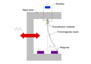
Figure 1: Illustration of the bistable piezo-magneto-elastic energy harvesting system.

Although this system dissipates energy, instead of using it to supply some secondary system, it is a typical prototype of a piezoelectric energy harvesting system. In an application of interest, the resistor is replaced by a more complex electrical circuit, which stores (and possibly manipulates) the voltage delivered by the mechanical system.

2.2 Initial value problem

The dynamic behavior of the system of interest is described by the following initial value problem

$$\ddot{x}+2\,\xi\,\dot{x}-\frac{1}{2}x\left(1-x^{2}\right)-\chi\,v=f\,\cos{\left(\Omega\,t\right)},$$ (1)

$$\dot{v}+\lambda\,v+\kappa\,\dot{x}=0,$$ (2)

$$x(0)=x_{0},\leavevmode\nobreak\ \dot{x}(0)=\dot{x}_{0},\leavevmode\nobreak\ v(0)=v_{0},$$ (3)

where $\xi$ is the damping ratio; $\chi$ is the piezoelectric coupling term in mechanical equation; $\lambda$ is a reciprocal time constant; $\kappa$ is the piezoelectric coupling term in electrical equation; $f$ is the external excitation amplitude; $\Omega$ is the external excitation frequency. The initial conditions are $x_{0}$, $\dot{x}_{0}$ and $v_{0}$, which respectively represent, the beam edge initial position, initial velocity and the initial voltage over the resistor. Also, $t$ denotes the time, so that the beam edge displacement at time $t$ is given by $x(t)$, and the resistor voltage at $t$ is represented by $v(t)$. The upper dot is an abbreviation for time-derivative, and all of these parameters are dimensionless.

2.3 Mean output power

Since the objective in this work is to maximize the amount of energy recovered by an energy harvesting process, the main quantity of interest (QoI) associated with the nonlinear dynamical system under analysis is the mean output power

$$P=\frac{1}{T_{f}-T_{0}}\int_{\tau=T_{0}}^{T_{f}}\lambda\,v^{2}(\tau)\,d\tau,$$ (4)

which is defined as the temporal average of the instantaneous power $\lambda\,v^{2}$ over a given time interval $[T_{0},T_{f}]$. This QoI plays the role of objective function in the optimization problem defined in section 3.

2.4 Dynamic classifier

Due to dynamical system nonlinearity, the steady-state dynamical response (over a given time interval) of the energy harvesting device may be chaotic or regular (non-chaotic), such as illustrated in Figure 2, which shows typical voltage time-series for this kind of bistable oscillator.

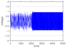
(a) regular dynamics

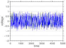
(b) chaotic dynamics

Figure 2: Two typical voltage time-series for the bistable energy harvesting system. The time-series in (a) has a regular steady-state dynamics, while in (b) a chaotic steady-state dynamics is observed.

To distinguish between the chaotic and regular dynamic regimes, the 0-1 test for chaos by Gottwald and Melbourne Gottwald and Melbourne (2004, 2009a, 2009b, 2016) is employed. This test, which is based on an extension of the dynamical system to a two-dimensional Euclidean group Bernardini and Litak (2016), uses a binary classifier $K$ to identify the dynamic regime of operation underlying the system of interest. This classifier is constructed from a dynamical system observation (time-series) $\phi(t)$. In fact, it is sufficient to use $\bm{\Phi}=\left(\phi(t_{1}),\phi(t_{2}),\cdots,\phi(t_{N})\right)$, a discrete version of the observable $\phi(t)$ that is obtained through a numerical integration (sampling) process.

Receiving the discrete observation (time-series) as an input, the analytical procedure of the 0-1 test consists of the following steps:

1. A real parameter $c\in[0,2\pi)$ is chosen and, for $n=1,2,\cdots,N$, the discrete version of $\phi(t)$ is used to define the translation variables

   $$p_{n}(c)=\sum_{j=1}^{n}\phi(t_{j})\,\cos{(j\,c)},$$ (5)

   $$q_{n}(c)=\sum_{j=1}^{n}\phi(t_{j})\,\sin{(j\,c)}.$$ (6)

2. Then, for $n=1,2,\cdots,N$, the time-averaged mean square displacement of the dynamics trajectory in $(p_{c},q_{c})$ space is computed by

   $$M_{n}(c)=\lim_{N\to\infty}\frac{1}{N}\,\sum_{j=1}^{N}\tilde{M}_{n}(c),$$ (7)

   where

   $$\tilde{M}_{n}(c)=\left(p_{j+n}(c)-p_{j}(c)\right)^{2}+\left(q_{j+n}(c)-q_{j}(c)\right)^{2}.$$ (8)

3. Finally, defining the mean-square vector

   $$\bm{\mbox{M}}_{n}=\left(M_{1},M_{2},\cdots,M_{n}\right),$$ (9)

   and the temporal mesh vector

   $$\bm{\mbox{t}}_{n}=\left(t_{1},t_{2},\cdots,t_{n}\right),$$ (10)

   the dynamic classifier is constructed through the correlation

   $$K_{c}=\lim_{n\to\infty}\frac{\texttt{cov}\left(\bm{\mbox{t}}_{n},\bm{\mbox{M}}_{n}\right)}{\sqrt{\texttt{var}\left(\bm{\mbox{t}}_{n}\right)\,\texttt{var}\left(\bm{\mbox{M}}_{n}\right)}},$$ (11)

   where $\texttt{cov}\left(\cdot,\cdot\right)$ and $\texttt{var}\left(\cdot\right)$ respectively denote the covariance and variance statistical operators.

It can be proved that $K_{c}\in\{0,1\}$, being $K_{c}=0$ for regular dynamics and $K_{c}=1$ for chaotic dynamics Gottwald and Melbourne (2009b); Bernardini and Litak (2016). For numerical implementation purposes, the above procedure is performed several times, for several randomly chosen values of $c\in[0,2\pi)$, and considering the voltage time-series as the system observation, i.e., $\phi(t)=v(t)$. The discrete version of $\phi(t)$ is constructed through temporal integration via the standard 4th order Runge-Kuta method. The limit processes in Eqs.(7) and (11) are replaced by the condition $n\ll N$, and the classifier $K$ is calculated as the median of $K_{c}$ realizations, i.e., $K=\texttt{median}\left(K_{c}\right)$. Indeed, for a careful done numerical simulation one has $K\approx 0$ or $K\approx 1$. See Bernardini and Litak (2016); Gottwald and Melbourne (2016) for further details.

3 Non-convex optimization problem

3.1 Problem definition

The objective of this work is to find a set of parameters that maximize the mean output power dissipated in the resistor. For this purpose, the electromechanical system properties ($\xi$, $\chi$, $\lambda$ and $\kappa$) sound as natural choices for the design variables, once they are intrinsic to the energy harvester embedded physical characteristics, something a designer might want to modify for better performance. However, the present work uses, first, the dynamical system excitation parameters, namely the amplitude $f$ and the frequency $\Omega$, as design variables. Although this choice sounds quite artificial at first since, in general, the designer does not have control of the level (or frequency) of vibration in which the energy harvester is operating, it is also of interest in the optimization of these systems to know in which vibration settings the device can recover more energy. As the numerical methodology developed here is completely general, it can be easily applied in the cases where the other parameters are used as the design variables, but by using $f$ and $\Omega$ to test the proposed methodology, an advantage is gained in terms of physical intuition about underlying physics, as the literature presents better knowledge about the effect of these two parameters on the behavior of this bistable energy harvesting system.

Many combinations of $(f,\Omega)$ lead the dynamical system to operate in the chaotic regime, an undesirable condition for electric power usage in principle, since the process of rectifying the chaotic electrical signal, which is necessary to enable its use in applications, can consume a significant part of the available energy. Although it is possible to explore the chaotic dynamics in favor of greater efficiency of the system Barbosa et al. (2015); Daqaq et al. (2020), as done by the author and collaborators in de la Roca et al. (2019), through the use of chaos control techniques, this is not the approach followed in the present work, which seeks to develop a very general numerical framework.

Thus, as not every pair $(f,\Omega)$ is an acceptable choice for the optimal design, it is necessary to impose a constraint that ensures the regularity (non-chaoticity) of the system dynamics. Taking advantage of the 0-1 test for chaos, described in section 2.4, the constraint to ensure a regular (non-chaotic) dynamic regime can be formulated as $K=0$. Note that the optimization problem is extremely nontrivial, once the constraint presents jump-type discontinuities since $K\in\{0,1\}$.

3.2 Constrained problem formulation

In an abstract way, one can formulate the constrained nonlinear optimization problem described above as find a feasible vector of design variables $\bm{\mbox{x}}^{\star}$ that maximize a certain objective function $\bm{\mbox{x}}\in\mathcal{D}\mapsto\mathcal{S}(\bm{\mbox{x}})\in\mathbb{R}$, i.e.,

$$\bm{\mbox{x}}^{\star}=\arg\max_{\bm{\mbox{x}}\in\mathcal{D}}{\,\mathcal{S}(\bm{\mbox{x}})},$$ (12)

where the set of admissible (feasible) parameters is defined by the bounded region

$$\mathcal{D}=\left\{\bm{\mbox{x}}\,\,|\,\,\bm{\mbox{x}}_{min}\leq\bm{\mbox{x}}\leq\bm{\mbox{x}}_{max}\leavevmode\nobreak\ \leavevmode\nobreak\ \mbox{and}\leavevmode\nobreak\ \leavevmode\nobreak\ \mathcal{G}(\bm{\mbox{x}})=0\right\}.$$ (13)

In this context, it is straightforward to see that the design variables vector is $\bm{\mbox{x}}=(f,\Omega)$, the objective function is $\mathcal{S}(\bm{\mbox{x}})=P(f,\Omega)$, the binary constraint is $\mathcal{G}(\bm{\mbox{x}})=K(f,\Omega)$, and the limits of the design variables are $\bm{\mbox{x}}_{min}=(f_{min},\Omega_{min})$ and $\bm{\mbox{x}}_{max}=(f_{max},\Omega_{max})$.

In the case of a problem with more variables, or with different objective function and/or constraints, the adaptations to be made are straightforward.

3.3 Penalized problem formulation

A penalized version of this constrained nonlinear optimization problem is introduced here in order to facilitate the computational implementation of the solution algorithm. In this formulation the constraint $\mathcal{G}(\bm{\mbox{x}})=0$ is replaced by the weaker condition $\mathcal{G}(\bm{\mbox{x}})\leq\varepsilon\ll 1$, once in practice the best one has is $K\approx 0$. In this way, the problem defined by (12) is replaced by the penalized problem which seeks a pair $\bm{\mbox{x}}^{\star}$ such that

$$\bm{\mbox{x}}^{\star}=\arg\max_{\bm{\mbox{x}}\in\mathcal{D}}{\tilde{\mathcal{S}}(\bm{\mbox{x}})},$$ (14)

where the set of feasible parameters is now defined by

$$\mathcal{D}=\left\{\bm{\mbox{x}}\,\,|\,\,\bm{\mbox{x}}_{min}\leq\bm{\mbox{x}}\leq\bm{\mbox{x}}_{max}\right\},$$ (15)

and the penalized objective function is given by

$$\tilde{\mathcal{S}}(\bm{\mbox{x}})=\mathcal{S}(\bm{\mbox{x}})\,-\,\alpha\,\max\left\{0,\mathcal{G}(\bm{\mbox{x}})\,-\,\varepsilon\right\}.$$ (16)

The penalty parameter is heuristically chosen, being $\alpha=10$ the value used in all simulations reported in this work. In the same way, $\varepsilon=1/10$ is adopted.

4 The cross-entropy method

4.1 The general idea of CE method

The key idea of the CE method is to transform the given non-convex optimization problem into an “equivalent” rare event estimation problem, that can be efficiently treated by a Monte Carlo like algorithm. The only requirement is that the problem has a single solution, i.e., the global extreme is unique.

In this framework, the feasible region is sampled according to a given probability distribution chosen by the user, and the low-order statistics (mean and standard deviation) of these samples are used to update the optimum point estimation, and the stopping criteria metric (respectively). This is a two-step iterative process:

1. Sampling: First, the feasible region is sampled according to a given probability distribution, and then the objective function is evaluated in each one of these samples. The information embedded in these samples are used in the algorithm adaptive process;

2. Learning: A special subset of these samples, dubbed the elite sample set, is defined by the samples that produced the highest values for the objective function. The parameters of the probability distribution are updated using statistics obtained from this elite sample set, modifying the given distribution in a sense that tries to make it as close as possible to a Dirac delta centered on the global optimum.

Throughout this process, the distribution mean provides the approximation for the global optimum. Its update is done in the sense of moving the distribution center towards the optimization problem optimum, while the standard deviation is reduced, thus “shrinking” the distribution around its central value. The continuous composition of these effects of translation and “shrinking” characterizes the process in which the distribution is “shaped” towards a point mass Dirac distribution centered on the optimal.

4.2 Theoretical framework

Without loss of generality, suppose that the problem of interest is to maximize an objective function $\bm{\mbox{x}}\in\mathcal{D}\mapsto\mathcal{S}(\bm{\mbox{x}})\in\mathbb{R}$, as stated in Eqs.(12). If the penalized formulation from Eq.(14) is adopted, just consider $\bm{\mbox{x}}\in\mathcal{D}\mapsto\tilde{\mathcal{S}}(\bm{\mbox{x}})\in\mathbb{R}$ instead of $\mathcal{S}(\bm{\mbox{x}})$.

Denote the global optimal by $\bm{\mbox{x}}^{\star}$ and the corresponding maximum value by $\gamma^{\star}=\mathcal{S}(\bm{\mbox{x}}^{\star})$, i.e., $\gamma^{\star}=\max{\,\mathcal{S}(\bm{\mbox{x}})}$ for all $\bm{\mbox{x}}\in\mathcal{D}$.

Using this global maximum as a reference value, and considering a randomized version of the vector x, denoted by X, it is possible construct the random event $\mathcal{S}(\bm{\mbox{X}})\geq\gamma^{\star}$, which represents the scenarios where the random variable $\mathcal{S}(\bm{\mbox{X}})$ is bigger or equal to the (deterministic) scalar value $\gamma^{\star}$. In other words, this random event considers the possibility of choosing, randomly, points in the feasible region $\mathcal{D}$ that produce values greater than or equal to the global maximum. Note that this random event is related to the optimization problem defined in Eq.(12), it can be thought of as its randomized version.

Since $\gamma^{\star}$ is the maximum value of $\mathcal{S}(\bm{\mbox{x}})$, no realization of X can produce $\mathcal{S}(\bm{\mbox{X}})>\gamma^{\star}$ and only $\bm{\mbox{X}}=\bm{\mbox{x}}^{\star}$ can make $\mathcal{S}(\bm{\mbox{X}})=\gamma^{\star}$. Therefore, the probability of this random event is zero, i.e., $\mathcal{P}\left\{\mathcal{S}(\bm{\mbox{X}})\geq\gamma^{\star}\right\}=0$.

Relaxing the reference value for a scalar $\gamma<\gamma^{\star}$, one has the random event $\mathcal{S}(\bm{\mbox{X}})\geq\gamma$, which defines a rare event if $\gamma\approx\gamma^{\star}$, for which $\mathcal{P}\left\{\mathcal{S}(\bm{\mbox{X}})\geq\gamma\right\}\approx 0$.

In his 1997 seminal work Rubinstein (1997), R. Rubinstein conceived the CE method as a tool to efficiently estimate such type of probabilities, associated with events located at the distribution tail. Sometime later Rubinstein (1999), due to the connection between the random event and the optimization problem described above, he noticed that this rare event estimation process could be used as a global search method to optimize the given objective function.

Notice that, with the aid of the expected value operator $\mathbb{E}\left\{\cdot\right\}$, and the indicator function

$$\mathds{1}_{\mathcal{A}}(\bm{\mbox{x}})=\begin{cases}1,\leavevmode\nobreak\ \mbox{if}\leavevmode\nobreak\ \bm{\mbox{x}}\in\mathcal{A}\\ 0,\leavevmode\nobreak\ \mbox{if}\leavevmode\nobreak\ \bm{\mbox{x}}\notin\mathcal{A}\,,\\ \end{cases}$$ (17)

the probability of the random event $\mathcal{S}(\bm{\mbox{X}})\geq\gamma$ can be written as

$$\mathcal{P}\left\{\mathcal{S}(\bm{\mbox{X}})\geq\gamma\right\}=\mathbb{E}\left\{\mathds{1}_{\mathcal{S}(\bm{\mbox{X}})\geq\gamma}\right\},$$ (18)

which provides a practical way of estimating its value. Once the right side of Eq.(18) is the mean value of the random event $\mathds{1}_{\mathcal{S}(\bm{\mbox{X}})\geq\gamma}$, it can be easily computed through the sample mean of $N_{s}$ samples of X, i.e.,

$$\mathbb{E}\left\{\mathds{1}_{\mathcal{S}(\bm{\mbox{X}})\geq\gamma}\right\}\approx\frac{1}{N_{s}}\,\displaystyle\sum_{k=0}^{N_{s}}\mathds{1}_{\mathcal{S}(\bm{\mbox{X}}_{k})\geq\gamma}\,,$$ (19)

where the realizations $\bm{\mbox{X}}_{k}$ ($k=1,\cdots,N_{s}$) are drawn according to $g\,(\bm{\mbox{x}};\bm{\mbox{v}})$, the probability density function of X, parametrized by the hyper-parameters vector v. Very often, $\bm{\mbox{v}}=(\bm{\mu},\bm{\sigma})$, where $\bm{\mu}$ and $\bm{\sigma}$ are the the mean the standard deviation vectors of X, respectively.

The idea of the CE method is to approximate the solution of the underlying optimization problem by solving the rare event probability estimation from Eq.(18). For this purpose, it employs a multilevel approach, that generates an optimal sequence of statistical estimators for the pair $(\gamma,\bm{\mbox{v}})$, denoted by $\left(\widehat{\gamma}_{\ell},\widehat{\bm{\mbox{v}}}_{\ell}\right)$, such that

$$\widehat{\gamma}_{\ell}\xrightarrow{\leavevmode\nobreak\ a.s.\leavevmode\nobreak\ }\gamma^{\star}\leavevmode\nobreak\ \leavevmode\nobreak\ \mbox{and}\leavevmode\nobreak\ \leavevmode\nobreak\ g\,(\bm{\mbox{x}},\widehat{\bm{\mbox{v}}}_{\ell})\xrightarrow{\leavevmode\nobreak\ a.s.\leavevmode\nobreak\ }\delta\left(\bm{\mbox{x}}-\bm{\mbox{x}}^{\star}\right),$$ (20)

i.e., the reference level $\gamma$ tends with probability 1 to the maximum value, and the family of distributions $g(\cdot\,,\,\bm{\mbox{v}})$ goes (almost sure) towards a point mass distribution, centered on the optimization problem global optimum.

This sequence of estimators is optimal in the sense that it minimizes the Kullback-Leibner divergence between $\mathds{1}_{\mathcal{S}(\bm{\mbox{X}})\geq\gamma}$ and $g(\cdot\,,\,\bm{\mbox{v}})$ Rubinstein and Kroese (2016).

More concretely, the feasible region $\mathcal{D}$ is sampled with $N_{s}$ independent and identically distributed (iid) realizations of the random vector X, drawn from its density $g\,(\bm{\mbox{x}};\bm{\mbox{v}})$. For each of these samples, the objective function is evaluated, generating the sequence of values $\mathcal{S}(\bm{\mbox{X}}_{1}),\mathcal{S}(\bm{\mbox{X}}_{2}),\cdots,\mathcal{S}(\bm{\mbox{X}}_{N_{s}})$.

Then, an elite sample $\mathcal{E}_{t}=\left\{\bm{\mbox{X}}_{k}\mathrel{\mathop{\mathchar 58\relax}}\mathcal{S}(\bm{\mbox{X}}_{k})\geq\widehat{\gamma}_{t}\right\}$ is defined by lumping the $N_{e}<N_{s}$ points that better performed, i.e., those which produced the highest values for $\mathcal{S}(\bm{\mbox{x}})$. Note that this elite set is defined in terms of the maximum value statistical estimator, given by

$$\widehat{\gamma}_{t}=\mathcal{S}_{(N_{s}-N_{e}+1)}.$$ (21)

The hyper-parameters vector v is updated using the maximum likelihood estimator so that, with the aid of the elite set $\mathcal{E}_{t}$, it is written as

$$\widehat{\bm{\mbox{v}}}_{t}=\arg\,\max_{\bm{\mbox{v}}}\,\sum_{\bm{\mbox{X}}_{k}\in\mathcal{E}_{t}}\ln\left(g\,(\bm{\mbox{X}}_{k};\bm{\mbox{v}})\right).$$ (22)

Depending on the distribution chosen for X, the stochastic program from Eq.(22) needs to be solved numerically. However, for the distributions of the exponential family, which includes the Gaussian and its truncated version, this estimator can be calculated in a analytic way, with each component of mean and deviation given by the formulas

$$\widehat{\mu}_{t}=\frac{\displaystyle\sum_{\bm{\mbox{X}}_{k}\in\mathcal{E}_{t}}X_{k}}{N_{e}},$$ (23)

and

$$\widehat{\sigma}_{t}=\sqrt{\frac{\displaystyle\sum_{\bm{\mbox{X}}_{k}\in\mathcal{E}_{t}}\left(X_{k}-\widehat{\mu}_{t}\right)^{2}}{N_{e}}},$$ (24)

respectively.

Although this process has a theoretical guarantee of converging to a point mass distribution centered on the global optimum, in computational practice it is common to see the updated distribution numerically degenerating before it “reaches the target”. Sometimes the standard deviation decreases very quickly, causing the distribution to “shrinks” in a region far from the global optimum. In this scenario, only samples far from the optimum point are drawn, producing poor estimates for the optimization problem solution.

At the theoretical level, where it is possible to sample an infinite number of times, this pathological situation is bypassed, because at some moment a sample on the tail is drawn, moving the distribution center out of the “frozen region”, as this outlier has a lot of weight in the mean estimate. However, in computational terms, as any robust implementation requires a maximum number of iterations (levels), the algorithm may stop with the distribution center within a “frozen region”.

This problem may be solved through the use of a smooth updating scheme for the hyper-parameters

$$\widehat{\bm{\mu}}_{t}\mathrel{\mathop{\mathchar 58\relax}}=\alpha\,\widehat{\bm{\mu}}_{t}+(1-\alpha)\,\widehat{\bm{\mu}}_{t-1},$$ (25)

$$\widehat{\bm{\sigma}}_{t}\mathrel{\mathop{\mathchar 58\relax}}=\beta_{t}\,\widehat{\bm{\sigma}}_{t}+(1-\beta_{t})\,\widehat{\bm{\sigma}}_{t-1},$$ (26)

$$\beta_{t}=\beta-\beta\,\left(1-\frac{1}{t}\right)^{q},$$ (27)

where the smooth parameters are such that $0<\alpha\leq 1$, $0.8\leq\beta\leq 0.99$ and $5\leq q\leq 10$ Kroese et al. (2011); Rubinstein and Kroese (2004), and the estimations at $t$ and $t-1$ are obtained by solving the Eq.(22), which defines the nonlinear program that gives rise to the vector v.

4.3 The computational algorithm

The geometric idea of the CE method is described at the beginning of this section, being complemented by the theoretical formalism presented in the previous subsection. The compilation of these ideas in the form of an easy to implement computational algorithm is presented below:

1. Define the number of samples $N_{s}$, the number of elite samples $N_{e}<N_{s}$, a convergence tolerance tol, the maximum of iteration levels $\ell_{max}$, a family of probability distributions $g\left(\cdot,\bm{\mbox{v}}{}\right)$, an initial vector of hyper-parameters $\widehat{\bm{\mbox{v}}}_{0}$ for $g$, and set the level counter $\ell=0$;

2. Update the level counter $\ell=\ell+1$;

3. Generate a total of $N_{s}$ independent and identically distributed (iid) samples from $g\left(\cdot,\widehat{\bm{\mbox{v}}}_{\ell-1}\right)$, denoted by $\bm{\mbox{X}}_{1},\cdots,\bm{\mbox{X}}_{N_{s}}$;

4. Evaluate the objective function $\mathcal{S}(\bm{\mbox{x}})$ at the samples $\bm{\mbox{X}}_{1},\cdots,\bm{\mbox{X}}_{N_{s}}$, sort the results $\mathcal{S}_{(1)}\leq\cdots\leq\mathcal{S}_{(N_{s})}$, and define the elite sample set $\mathcal{E}_{t}$ with the $N_{e}$ points which better performed;

5. Update the estimators $\widehat{\gamma}_{\ell}$ and $\widehat{\bm{\mbox{v}}}_{\ell}$ with aid of the elite sample set, using order and maximum likelihood statistic estimators, given by the Eqs.(21) and (22), respectively. If necessary, apply the scheme of smooth updating;

6. Repeat the steps (2) up to (5) of this algorithm while a (standard deviation dependent) stopping criterion is not met. For instance, $\max\left\{\bm{\sigma}\right\}<\texttt{tol}$.

A schematic representation of this algorithm, illustrating all the stages of the sampling and learning phases, can be seen in Figure 3.

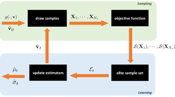
Figure 3: Schematic representation of the CE algorithm for optimization.

4.4 Remarks about CE method

Among the several characteristics that make this relatively novel technique interesting, the following can be highlighted:

• Simplicity – very intuitive algorithm with few control parameters ($N_{s}$, $N_{e}$, $\ell_{max}$ and tol), each of then with a very clear interpretation;

• Robustness – theoretical results ensure that, under typical conditions, the method is guaranteed to converge if the problem has a single global extreme;

• Efficiency – the method typically presents fast convergence in comparison with classic global search meta-heuristics, such as genetic algorithms;

• Generality – the method does not require any regularity of the objective function and can be applied to almost any type of non-convex optimization problem (even non-differentiable or discontinuous);

• Extensibility – the theory is general, in principle it can be applied to problems of any finite dimension, the computational cost and the “curse of dimensionality” being the limiting factors in practice;

• Easy implementation – the algorithm can be implemented with a few lines of code in a high level programming language.

The mathematical development associated with the formalism described above is relatively non-trivial, but it has been well established throughout the first decade of the method, including theorems that strictly establish the conditions where the method has guaranteed convergence. These details are suppressed from this paper as they are outside the scope of the journal. But for the interested reader, the following references are recommended De Boer et al. (2005); Kroese et al. (2011); Rubinstein and Kroese (2004, 2016).

The computational experiments in the next section illustrate the efficiency and robustness of this framework in solving a non-trivial problem of optimizing an energy harvesting device.

5 Numerical experiments

For the numerical experiments conducted here, the following numerical values are adopted for the dynamical system parameters: $\xi=0.01$, $\chi=0.05$, $\kappa=0.5$ and $\lambda=0.05$. The initial condition is defined by $x_{0}=1$, $\dot{x}_{0}=0$ and $v=0$. The dynamics is integrated over the time interval $[0,2500]$, and the mean output power is computed over the last 50% of this time-series, i.e., $[T_{0},T_{f}]=[1250,2500]$.

5.1 Reference solution

In order to analyze the effectiveness and robustness of the stochastic solution strategy proposed here, a reference solution is computed by a standard exhaustive search on a fine grid over the domain

$$\mathcal{D}=\left\{(f,\Omega)\,|\,0.08\leq f\leq 0.1,\,0.75\leq\Omega\leq 0.85\right\}.$$

In this standard approach, a structured 256 x 256 uniform numerical grid is used to discretize $\mathcal{D}$. The system dynamics is then integrated for each grid point, with the optimization constraint being evaluated next. The objective function is evaluated at all feasible points, and the extreme value is updated at each step of the grid screening process. Two contour maps, associated with the reference solution, are shown in Figure 4: (a) constraint function, and (b) objective function normalized by $P_{max}^{DS}$. The pair $(f,\Omega)=(0.0999,0.7786)$ that corresponds to the global maximum is indicated in both contour maps by a red cross, being associated with a mean output power $P_{max}^{DS}=0.0172$. Figure 5 shows a magnification of the global maximum neighborhood, where it is possible to better appreciate the contour levels shape, and verify that it corresponds to a regular dynamic regime configuration. Note also that this result is compatible with the literature, which points to a better performance of piezoelectric harvesters for low frequencies and high amplitudes of excitation Lopes et al. (2019a); Vocca et al. (2012). For sake of reference, this solution was obtained in 3.6 hours in a Dell Inspiron Core i7-3632QM 2.20 GHz RAM 12GB.

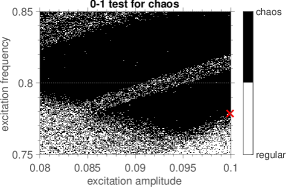
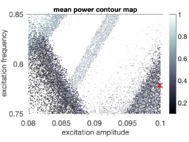
Figure 4: Bi-dimensional case contour maps: (a) constraint function defined by the 0-1 test for chaos, and (b) normalized objective function, defined by the mean output power.

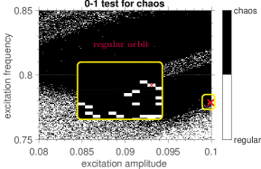
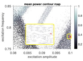
Figure 5: Magnification of the contour maps in bi-dimensional case: (a) constraint function defined by the 0-1 test for chaos, and (b) normalized objective function, defined by the mean output power.

5.2 Cross-entropy solution

In the approach based on the CE method, the domain is randomly sampled using for this $N^{s}=50$ points. This sampling is done according to a truncated Gaussian distribution, parametrized by mean vector $\bm{\mu}=(\mu_{f},\mu_{\Omega})$ and standard deviation vector $\bm{\sigma}=(\sigma_{f},\sigma_{\Omega})$. The number of elite samples is chosen as $N^{e}=\texttt{round}(N^{s}/10)$, maximum number of levels is set $t_{max}=100$, while the convergence criterion is adopted as $\max{\left\{\sigma_{f},\sigma_{\Omega}\right\}}<\texttt{tol}$, for a tolerance $\texttt{tol}=1\times 10^{-3}$. The smoothing parameters are $\alpha=0.7$, $\beta=0.8$ and $q=5$.

A visual illustration of the CE method is presented in Figure 6, which shows the domain sampling at different levels (iterations) of the algorithm. The reader can also appreciate the evolution of this random algorithm in Table 1, where each line displays the level index, the value of the means and standard deviations of $f$ and $\Omega$ in addition to the optimal value obtained for the objective function $P$ and the corresponding constraint $K$. In this case, the optimum value obtained by the CE method, with aid of the estimation from Eq.(21), is $P_{max}^{CE}=0.0170$, at the optimal point $\bm{\mbox{x}}^{\star}=(f^{\star},\Omega^{\star})$ where $f^{\star}\approx 0.10$ and $\Omega^{\star}\approx 0.77$.

Table 1: Evolution of CE algorithm in the bi-dimensional case using $N^{s}=50$ samples.

$\ell$	$P$	$K$	$\mu_{f}$	$\mu_{\Omega}$	$\sigma_{f}$	$\sigma_{\Omega}$
01	0.0151	0.1115	0.0858	0.7845	0.0260	0.1107
02	0.0003	0.0195	0.0872	0.7804	0.0115	0.0498
03	0.0004	0.0956	0.0901	0.7687	0.0084	0.0260
04	0.0003	0.0610	0.0913	0.7674	0.0061	0.0205
05	0.0004	0.0969	0.0914	0.7706	0.0059	0.0208
06	0.0003	0.0054	0.0917	0.7635	0.0053	0.0152
07	0.0004	0.0444	0.0916	0.7601	0.0048	0.0104
08	0.0169	0.0264	0.0955	0.7643	0.0036	0.0068
09	0.0167	0.0662	0.0966	0.7618	0.0031	0.0058
10	0.0167	0.0121	0.0975	0.7629	0.0024	0.0053
11	0.0168	0.0437	0.0977	0.7649	0.0021	0.0042
12	0.0169	0.0208	0.0981	0.7671	0.0018	0.0035
13	0.0169	0.0230	0.0985	0.7684	0.0016	0.0028
14	0.0169	0.0151	0.0990	0.7686	0.0013	0.0023
15	0.0170	0.0338	0.0989	0.7702	0.0011	0.0022
16	0.0170	0.0476	0.0990	0.7716	0.0010	0.0020
17	0.0171	0.0319	0.0994	0.7731	0.0009	0.0018
18	0.0170	0.0001	0.0995	0.7724	0.0008	0.0017
19	0.0171	0.0088	0.0994	0.7729	0.0007	0.0016
20	0.0171	0.0053	0.0994	0.7736	0.0007	0.0014
21	0.0171	0.0825	0.0994	0.7739	0.0006	0.0014
22	0.0171	0.0109	0.0995	0.7741	0.0006	0.0013
23	0.0171	0.0165	0.0995	0.7741	0.0006	0.0012
24	0.0150	0.3716	0.0994	0.7730	0.0005	0.0011
25	0.0171	0.0033	0.0995	0.7734	0.0005	0.0010
26	0.0170	0.0578	0.0995	0.7732	0.0004	0.0010

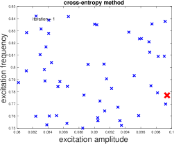
(a) $\ell=1$

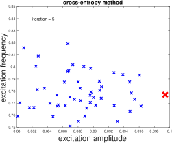
(b) $\ell=5$

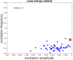
(c) $\ell=9$

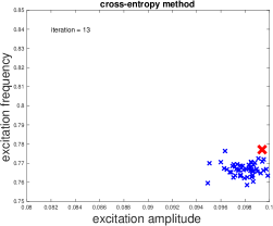
(d) $\ell=13$

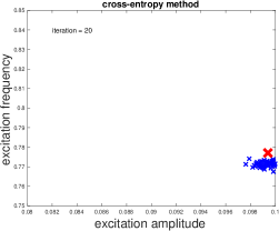
(e) $\ell=20$

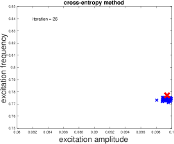
(f) $\ell=26$

Figure 6: Illustration of CE method in the bi-dimensional case, using $N^{s}=50$ samples, at different levels (iterations) of the algorithm. The reference solution is indicated with a red cross.

Table 2: Performance of CE algorithm in the bi-dimensional case for different number of samples.

samples	levels	CPU time*	speed-up	function
		(seconds)		evaluation
reference	—	13 101	—	65 536
25	19	106	123	475
50	26	287	46	1 300
75	30	497	26	2 250
100	28	610	21	2 800

*Dell Inspiron Core i7-3632QM 2.20 GHz RAM 12GB

Note that the approximation obtained is very close to the reference value of section 5.1, obtained after 26 iterative steps (1300 function evaluations), which corresponds to a speed-up of more than 40, when compared with the exhaustive search (see in Table 2 the CPU time spent). The accuracy can still be slightly improved as shown in Table 3, which presents the CE results with $N^{s}=75$, obtaining $P_{max}^{CE}=0.0171$. In this case, the price paid for this additional gain of accuracy is a loss of performance, which makes the speed-up fall from more than 40 to 26 (see Table 2). However, an experiment with only $N^{s}=25$ samples is also conducted, obtaining a result with no loss of accuracy and more than doubling the speed-up to an impressive value of 123. An experiment with $N^{s}=100$ is also reported in Table 2, although no figure or table from this simulation is shown in the text. This experiment shows that different sampling strategies can produce good results.

Table 3: Evolution of CE algorithm in the bi-dimensional case using $N^{s}=75$ samples.

$\ell$	$P$	$K$	$\mu_{f}$	$\mu_{\Omega}$	$\sigma_{f}$	$\sigma_{\Omega}$
01	0.0002	0.0636	0.0868	0.7883	0.0247	0.1244
02	0.0003	0.1676	0.0901	0.7712	0.0101	0.0355
03	0.0003	0.0224	0.0883	0.7683	0.0074	0.0187
04	0.0004	0.0181	0.0936	0.7634	0.0048	0.0119
05	0.0004	0.0448	0.0966	0.7597	0.0030	0.0082
06	0.0167	0.0358	0.0974	0.7628	0.0021	0.0065
07	0.0168	0.0425	0.0978	0.7651	0.0019	0.0052
08	0.0169	0.0533	0.0986	0.7679	0.0016	0.0041
09	0.0170	0.0473	0.0987	0.7705	0.0013	0.0035
10	0.0170	0.0177	0.0988	0.7705	0.0012	0.0029
11	0.0170	0.0415	0.0991	0.7706	0.0009	0.0024
12	0.0170	0.0519	0.0991	0.7716	0.0008	0.0021
13	0.0170	0.0173	0.0992	0.7717	0.0008	0.0021
14	0.0170	0.0867	0.0992	0.7727	0.0007	0.0021
15	0.0171	0.0349	0.0992	0.7733	0.0006	0.0020
16	0.0171	0.0427	0.0992	0.7735	0.0006	0.0018
17	0.0171	0.0234	0.0991	0.7736	0.0005	0.0016
18	0.0171	0.0077	0.0991	0.7739	0.0005	0.0015
19	0.0170	0.0742	0.0991	0.7734	0.0005	0.0013
20	0.0171	0.0049	0.0993	0.7736	0.0005	0.0012
21	0.0171	0.0085	0.0994	0.7737	0.0004	0.0012
22	0.0170	0.0806	0.0995	0.7737	0.0004	0.0013
23	0.0171	0.0272	0.0995	0.7742	0.0004	0.0012
24	0.0171	0.0370	0.0996	0.7742	0.0004	0.0011
25	0.0171	0.0485	0.0996	0.7741	0.0003	0.0011
26	0.0171	0.0099	0.0995	0.7745	0.0003	0.0011
27	0.0151	0.0857	0.0996	0.7744	0.0003	0.0011
28	0.0171	0.0532	0.0996	0.7749	0.0003	0.0010
29	0.0171	0.0097	0.0996	0.7742	0.0003	0.0010
30	0.0171	0.0512	0.0995	0.7742	0.0003	0.0010

Table 4: Evolution of CE algorithm in the bi-dimensional case using $N^{s}=25$ samples.

$\ell$	$P$	$K$	$\mu_{f}$	$\mu_{\Omega}$	$\sigma_{f}$	$\sigma_{\Omega}$
01	0.0003	0.1251	0.0883	0.7870	0.0276	0.1106
02	0.0003	0.0095	0.0867	0.7692	0.0131	0.0352
03	0.0003	0.0522	0.0889	0.7658	0.0095	0.0181
04	0.0003	0.0822	0.0891	0.7608	0.0074	0.0131
05	0.0164	0.0347	0.0938	0.7596	0.0052	0.0111
06	0.0167	0.0451	0.0960	0.7604	0.0038	0.0077
07	0.0167	0.0341	0.0981	0.7620	0.0025	0.0056
08	0.0168	0.0415	0.0986	0.7656	0.0022	0.0051
09	0.0168	0.0845	0.0985	0.7666	0.0021	0.0049
10	0.0169	0.0061	0.0987	0.7674	0.0018	0.0035
11	0.0169	0.0007	0.0986	0.7662	0.0015	0.0029
12	0.0169	0.0453	0.0988	0.7671	0.0013	0.0023
13	0.0170	0.0648	0.0993	0.7684	0.0010	0.0019
14	0.0170	0.0569	0.0993	0.7700	0.0009	0.0017
15	0.0170	0.0226	0.0992	0.7707	0.0008	0.0014
16	0.0170	0.0497	0.0993	0.7710	0.0008	0.0012
17	0.0170	0.0716	0.0992	0.7714	0.0007	0.0013
18	0.0171	0.0226	0.0996	0.7723	0.0006	0.0012
19	0.0171	0.0089	0.0996	0.7730	0.0006	0.0010

The speed-up shown in Table 2 is defined as the ratio between the calculation time between direct search (reference) and the CE solution. Although this metric provides a good measure of efficiency for large values of CPU times, it is extremely dependent on the machine used. Thus, to provide a machine-independent performance measure, this table also lists the number of evaluations of the objective function, since this is the most expensive operation to be performed by the optimization algorithm. Note that in this new metric, the ratio between the objective function evaluations in the reference and the CE solution produces values very close to the speed-ups obtained previously, confirming the computational efficiency of the proposed approach in a machine-independent fashion.

An animation of the algorithm in action with $N^{s}=50$ is available in Cunha Jr (2020b), where the reader can see the algorithm stops after just $\ell=17$ levels (850 function evaluations). The difference concerning the numerical experiment reported in Table 1 is because the CE method is stochastic so that at each simulation, a different approximation for the global optimum is constructed. Despite these variations, the speed-up and function evaluation values reported in Table 1 are typical, with some fluctuation around them each new simulation, but with no change in the order of magnitude. Animations for the cases where $N^{s}=25$ and $N^{s}=75$ can be seen in Cunha Jr (2020a) and Cunha Jr (2020c), respectively, where it is possible to note that the accuracy and speed-ups obtained are comparable to those results shown in Tables 3 and 4.

5.3 Noise robustness

In the practical operation of a vibratory device, noise is inevitable, so considering its effect on the dynamics of energy harvesting systems is good modeling practice Lopes et al. (2019b). Therefore, robustness to noise is a desirable feature in any optimization methodology in problems involving dynamical systems. To test the robustness of the CE solution to noise disturbances, this section slightly modifies the reference solution from section 5.1. For that, the output voltage signal is corrupted with Gaussian white noise component (zero-mean and standard deviation equal to 5% of the maximum voltage amplitude). In this way, the objective function of the optimization problem becomes noisy, providing a more stringent test for the optimizer.

The contour maps of the constraint and the noisy objective function, with their respective magnifications, both constructed on the same $256\times 256$ numerical grid from section 5.1 (CPU time 3.8 hours), can be seen in Figure 7. Note that the noise disturbance changes the geometry of the constraint contour map, expanding the regions of chaotic configuration. It also affects the mean power isolines, thus changing a little bit the objective function, so that $P_{max}^{DS}=0.0173$ at $(f,\Omega)=(0.0998,0.7763)$.

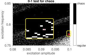
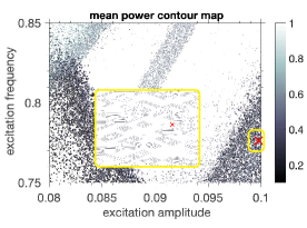
Figure 7: Noisy case contour maps: (a) constraint function defined by the 0-1 test for chaos, and (b) noisy objective function defined by the mean output power.

In this noisy experiment, the CE method uses $N^{s}=50$, tolerance $\texttt{tol}=1/512$, and all other parameters set as in the noiseless case. In this way, the CE method finds, after 25 iterations, $P_{max}^{CE}=0.0170$ at the pair $(f,\Omega)=(0.0991,0.7675)$, which is a very accurate approximation of the reference solution presented above. An illustration of this iterative process is shown in Figure 8. Note that here the CE algorithm constructs the approximation for the optimum by a different path than the one shown in Figure 6.

Even though the presence of noise complicates the penalized objective function assessment, the example above shows that the CE method may be able to find an accurate approximation for the global optimum. But a caveat needs to be made. Depending on the chosen tolerance value, the CE method may “froze in a certain region”. For this experiment, for example, a solution with an accuracy defined by $\texttt{tol}=0.001<1/512$ cannot be reached in $\ell_{max}=100$ iterations, as the approximations “freeze” in a region close to, but not close enough to, the global optimum. In practical terms, this can be a limitation, which depends on the problem at hand.

(a) $\ell=1$

(b) $\ell=5$

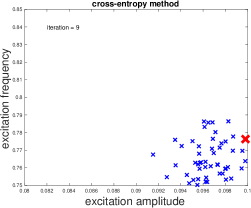
(c) $\ell=9$

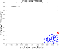
(d) $\ell=13$

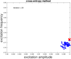
(e) $\ell=20$

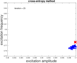
(f) $\ell=25$

Figure 8: Illustration of CE method in the noisy case, using $N^{s}=50$ samples, at different levels (iterations) of the algorithm. The noisy version of reference solution is indicated with a red cross.

5.4 Multidimensional optimization

In principle, the CE method is extensible to any finite dimension. However, in practice, the CE method suffers from a pathology known as the “curse of dimensionality”, which is the significant drop of the CE estimator accuracy as the number of design variables increase Rubinstein and Glynn (2009). Although an improved CE algorithm, that can partially mitigate this problem, exists in the literature Rubinstein and Glynn (2009), it is not considered here since the paper aims to explore the simplest, and most intuitive, version of the CE method.

In the context of interest in this paper, optimal design of an energy harvester (and in a broader sense, in dynamic systems), the optimization problems generally have a few design variables, with a dimension of half a dozen being considered high. In this case, although less accurate than in the two-dimensional case, the solution obtained by the CE method can still be useful.

To illustrate this point, an example with 4 design variables, $\bm{\mbox{x}}=\left(\xi,\chi,\lambda,\kappa\right)$, is considered in this section, where $f=0.115$ and $\Omega=0.8$ are fixed and the feasible region is defined by

$$\mathcal{D}=[0.01,0.05]\times[0.05,0.2]\times[0.05,0.2]\times[0.5,1.5].$$

A reference solution is constructed via direct search on a $16\times 16\times 16\times 16$ uniform mesh defined in $\mathcal{D}$, where the global maximum $P_{max}^{DS}=0.1761$ is obtained at $\left(\xi,\chi,\lambda,\kappa\right)=(0.0340,0.0600,0.2000,1.5000)$. The computational budget spent to obtain this solution is similar to that of the direct search in section 5.1, involving 65 536 evaluations of the objective function. As now the feasible region has a higher dimension than in the two-dimensional example, it is expected that the direct search solution obtained will be less accurate. But this is not problematic for the analyzes presented here, even though it is less precise, this numerical solution is suitable for reference purposes.

Using the CE method in this case it is possible to speed-up the optimization process and obtain a approximation reasonably close to the global optimum. Table 5 shows the results obtained for different values of $N^{s}$, $\texttt{tol}=0.01$, and considering the other parameters of the algorithm as in section 5.2. In all scenarios, the solution obtained by the CE method corresponds to a mean power very close to the one obtained by the direct search in the numerical grid, with speed-up gains up to 30 times approximately. These results indicate that, even though it is susceptible to “curse of dimensionality”, the CE method can be a very appealing algorithm for problems in moderately higher dimensions, since it can provide accurate approximations and in a very competitive processing time.

Table 5: Performance of CE algorithm in the multidimensional case, for different number of samples ($\texttt{tol}=0.01$).

samples	levels	CPU time*	speed-up	function	$P_{max}$	$\xi$	$\chi$	$\lambda$	$\kappa$
		(seconds)		evaluation
reference	—	12 648	—	65 536	0.1761	0.0340	0.0600	0.2000	1.5000
100	75	2074	6	7 500	0.1612	0.0237	0.1053	0.1953	1.4923
50	59	696	18	2 950	0.1603	0.0227	0.1099	0.1938	1.4969
25	83	466	27	2 075	0.1619	0.0227	0.1062	0.1955	1.4924

*Dell Inspiron Core i7-3632QM 2.20 GHz RAM 12GB

5.5 Remarks on CE solution

The above results allow one to conclude that the optimization approach based on the CE method is robust (able to find the global optimal) and efficient (computationally feasible) to address this nonlinear non-convex optimization problem, which has non-trivial numerical solution since the existence of jump-like discontinuities in the constraint prevents gradient-based algorithms from being used.

Last but not least, it is worth mentioning that the CE method has a great advantage in terms of simplicity when compared to most of the meta-heuristics used in non-differentiable optimization since the algorithm involves only four control parameters, all of which have a very intuitive meaning, which is a considerable advantage compared to genetic algorithms for example.

6 Conclusions

This work presented the formulation of a nonlinear non-convex optimization problem that seeks to maximize the efficiency of a bistable energy harvesting system driven by a sinusoidal excitation and constrained to operate in non-chaotic dynamic regimes only. Since the problem has jump-type discontinuities, which prevents the use of gradient-based methods, a stochastic strategy of optimization, based on the cross-entropy method, was proposed to construct a numerical approximation for the optimal solution.

Tests to verify the efficiency and accuracy of this cross-entropy approach as well as its robustness to noise and feasibility of use in larger dimensions, were conducted. They showed that the proposed strategy of optimization is quite robust and effective, constituting a very appealing tool to deal with the typical (non-convex) problems related to the optimization of energy harvesting systems, even in the presence of noise or in a problem with moderately high dimension.

The impressive results reported here can still be improved in terms of performance, through the use of parallelization strategies. In particular, it would be interesting to test the cloud computing parallelization strategy proposed by Cunha Jr et al. (2014). Besides, the optimization framework is extremely versatile, allowing the extension to problems involving robust optimization such as those reported by Cunha Jr et al. (2015); Wolszczak et al. (2019), in which the global optimum is not sought in the strict sense, but in a sense in which the system performance is maximized in average terms, respecting probabilistic constraints.

Funding

This research received financial support from the Brazilian agencies Coordenação de Aperfeiçoamento de Pessoal de Nível Superior - Brasil (CAPES) - Finance Code 001, and the Carlos Chagas Filho Research Foundation of Rio de Janeiro State (FAPERJ) under the following grants: 211.304/2015, 210.021/2018, 210.167/2019, and 211.037/2019.

Compliance with ethical standards

Conflict of Interest

The author declares that he has no conflict of interest.

Code availability

To facilitate the reproduction of this paper results, as well as to popularize the CE method use by the community of nonlinear dynamical systems, the code used in the simulations is available in the following repository:
https://americocunhajr.github.io/HarvesterOpt

References

- Abdelkefi et al. (2012) Abdelkefi A, Nayfeh AH, Hajj MR (2012) Enhancement of power harvesting from piezoaeroelastic systems. Nonlinear Dynamics 68:531–541, DOI https://doi.org/10.1007/s11071-011-0234-9
- Barbosa et al. (2015) Barbosa WOV, De Paula AS, Savi MA, Inman DJ (2015) Chaos control applied to piezoelectric vibration-based energy harvesting systems. The European Physical Journal Special Topics 224:2787–2801, DOI https://doi.org/10.1140/epjst/e2015-02589-1
- Benacchio et al. (2016) Benacchio S, Malher A, Boisson J, Touzé C (2016) Design of a magnetic vibration absorber with tunable stiffnesses. Nonlinear Dynamics 85:893–911, DOI https://doi.org/10.1007/s11071-016-2731-3
- Bernardini and Litak (2016) Bernardini D, Litak G (2016) An overview of 0–1 test for chaos. Journal of the Brazilian Society of Mechanical Sciences and Engineering 38:1433–1450, DOI https://doi.org/10.1007/s40430-015-0453-y
- Bhatti et al. (2016) Bhatti NA, Alizai MH, Syed AA, L M (2016) Energy harvesting and wireless transfer in sensor network applications: Concepts and experiences. ACM Transactions on Sensor Networks 12:24:1–24:40, DOI https://doi.org/10.1145/2915918
- Bonnans et al. (2009) Bonnans J, Gilbert JC, Lemarechal C, Sagastizábal CA (2009) Numerical Optimization: Theoretical and Practical Aspects, 2nd edn. Springer
- Boyd and Vandenberghe (2004) Boyd S, Vandenberghe L (2004) Convex Optimization. Cambridge University Press
- Catacuzzeno et al. (2019) Catacuzzeno L, Orfei F, Michele AD, Sforna L, Franciolini F, Gammaitoni L (2019) Energy harvesting from a bio cell. Nano Energy 56:823–827
- Cottone et al. (2009) Cottone F, Vocca H, Gammaitoni L (2009) Nonlinear energy harvesting. Phys Rev Lett 102:080601, DOI https://doi.org/10.1103/PhysRevLett.102.080601
- Cunha Jr (2020a) Cunha Jr A (2020a) Cross-entropy optimization of bistable energy harvesting system (25 samples). https://youtu.be/0EvzdVXlPqA, (Accessed 28 March 2020)
- Cunha Jr (2020b) Cunha Jr A (2020b) Cross-entropy optimization of bistable energy harvesting system (50 samples). https://youtu.be/-JB3eniIdDY, (Accessed 28 March 2020)
- Cunha Jr (2020c) Cunha Jr A (2020c) Cross-entropy optimization of bistable energy harvesting system (75 samples). https://youtu.be/uIZM4SjCbrw, (Accessed 28 March 2020)
- Cunha Jr et al. (2014) Cunha Jr A, Nasser R, Sampaio R, Lopes H, Breitman K (2014) Uncertainty quantification through Monte Carlo method in a cloud computing setting. Computer Physics Communications 185:1355–1363, DOI https://doi.org/10.1016/j.cpc.2014.01.006
- Cunha Jr et al. (2015) Cunha Jr A, Soize C, Sampaio R (2015) Computational modeling of the nonlinear stochastic dynamics of horizontal drillstrings. Computational Mechanics 56:849–878, DOI https://doi.org/10.1007/s00466-015-1206-6
- Dantas (2019) Dantas E (2019) A cross-entropy strategy for parameters identification problems. Monograph, Universidade do Estado do Rio de Janeiro, https://dx.doi.org/10.13140/RG.2.2.18045.51688
- Dantas et al. (2019a) Dantas E, Cunha Jr A, Silva TAN (2019a) A numerical procedure based on cross-entropy method for stiffness identification. In: 5th International Conference on Structural Engineering Dynamics (ICEDyn 2019), Viana do Castelo, Portugal
- Dantas et al. (2019b) Dantas E, Cunha Jr A, Soeiro FJCP, Cayres BC, Weber HI (2019b) An inverse problem via cross-entropy method for calibration of a drill string torsional dynamic model. In: 25th ABCM International Congress of Mechanical Engineering (COBEM 2019), Uberlândia, Brazil, DOI http://dx.doi.org/10.26678/abcm.cobem2019.cob2019-2216
- Daqaq et al. (2020) Daqaq MF, Crespo RS, Ha S (2020) On the efficacy of charging a battery using a chaotic energy harvester. Nonlinear Dynamics 99:1525–1537, DOI https://doi.org/10.1007/s11071-019-05372-0
- De Boer et al. (2005) De Boer P, Kroese DP, Mannor S, Rubinstein RY (2005) A tutorial on the cross-entropy method. Annals of Operations Research 134:19–67, DOI https://doi.org/10.1007/s10479-005-5724-z
- de la Roca et al. (2019) de la Roca L, Peterson JVLL, Pereira MC, Cunha Jr A (2019) Control of chaos via OGY method on a bistable energy harvester. In: 25th ABCM International Congress of Mechanical Engineering (COBEM 2019), Uberlândia, Brazil, DOI http://dx.doi.org/10.26678/abcm.cobem2019.cob2019-1970
- Dekemele et al. (2019) Dekemele K, Van Torre P, Loccufier M (2019) Performance and tuning of a chaotic bi-stable nes to mitigate transient vibrations. Nonlinear Dynamics 98:1831–1851, DOI https://doi.org/10.1007/s11071-019-05291-0
- Erturk et al. (2009) Erturk A, Hoffmann J, Inman DJ (2009) A piezomagnetoelastic structure for broadband vibration energy harvesting. Applied Physics Letters 94:254102, DOI https://doi.org/10.1063/1.3159815
- Gallo et al. (2012) Gallo CA, Tofoli FL, Rade DA, Steffen, Jr V (2012) Piezoelectric actuators applied to neutralize mechanical vibrations. Journal of Vibration and Control 18:1650–1660, DOI https://doi.org/10.1177/1077546311422549
- Gammaitoni (2012) Gammaitoni L (2012) There’s plenty of energy at the bottom (micro and nano scale nonlinear noise harvesting). Contemporary Physics 53:119–135, DOI https://doi.org/10.1080/00107514.2011.647793
- Ghidey (2015) Ghidey H (2015) Reliability-based design optimization with cross-entropy method. Master’s thesis, Norwegian University of Science and Technology, Trondheim
- Ghouli et al. (2017) Ghouli Z, Hamdi M, Belhaq M (2017) Energy harvesting from quasi-periodic vibrations using electromagnetic coupling with delay. Nonlinear Dynamics 89:1625–1636, DOI https://doi.org/10.1007/s11071-017-3539-5
- Godoy and Trindade (2012) Godoy TC, Trindade MA (2012) Effect of parametric uncertainties on the performance of a piezoelectric energy harvesting device. Journal of the Brazilian Society of Mechanical Sciences and Engineering 34:552–560, DOI https://dx.doi.org/10.1590/S1678-58782012000600003
- Gottwald and Melbourne (2004) Gottwald GA, Melbourne I (2004) A new test for chaos in deterministic systems. Proceedings of the Royal Society of London Series A 460:603–611, DOI https://doi.org/10.1098/rspa.2003.1183
- Gottwald and Melbourne (2009a) Gottwald GA, Melbourne I (2009a) On the implementation of the 0-1 test for chaos. SIAM Journal on Applied Dynamical Systems 8:129–145, DOI https://doi.org/10.1137/080718851
- Gottwald and Melbourne (2009b) Gottwald GA, Melbourne I (2009b) On the validity of the 0-1 test for chaos. Nonlinearity 22:1367–1382, DOI https://doi.org/10.1088/0951-7715/22/6/006
- Gottwald and Melbourne (2016) Gottwald GA, Melbourne I (2016) The 0-1 Test for Chaos: A review, vol 915, Springer. DOI https://doi.org/10.1007/978-3-662-48410-4
- Harne (2012) Harne RL (2012) Theoretical investigations of energy harvesting efficiency from structural vibrations using piezoelectric and electromagnetic oscillators. The Journal of the Acoustical Society of America 132:162–172, DOI https://doi.org/10.1121/1.4725765
- Ibrahim et al. (2016) Ibrahim A, Towfighian S, Younis M, Su Q (2016) Magnetoelastic beam with extended polymer for low frequency vibration energy harvesting. In: Meyendorf NG, Matikas TE, Peters KJ (eds) Smart Materials and Nondestructive Evaluation for Energy Systems 2016, International Society for Optics and Photonics, SPIE, vol 9806, pp 71 – 85, DOI https://doi.org/10.1117/12.2219276
- Issa et al. (2018) Issa MVS, Cunha Jr A, Soeiro FJCP, Pereira A (2018) Structural optimization using the cross-entropy method. In: XXXVIII Congresso Nacional de Matemática Aplicada e Computacional (CNMAC 2018), Campinas, Brazil, DOI https://dx.doi.org/10.5540/03.2018.006.02.0443
- Kroese et al. (2011) Kroese DP, Taimre T, Botev ZI (2011) Handbook of Monte Carlo Methods. Wiley
- Kroese et al. (2013) Kroese DP, Rubinstein RY, Cohen I, Porotsky S, Taimre T (2013) Cross-Entropy Method, Springer, pp 326–333. DOI https://doi.org/10.1007/978-1-4419-1153-7˙131
- Leadenham and Erturk (2020) Leadenham S, Erturk A (2020) Mechanically and electrically nonlinear non-ideal piezoelectric energy harvesting framework with experimental validations. Nonlinear Dynamics 99:625–641, DOI https://doi.org/10.1007/s11071-019-05091-6
- Liu et al. (2019) Liu W, Xu X, Chen F, Liu Y, Li S, Liu L, Chen Y (2019) A review of research on the closed thermodynamic cycles of ocean thermal energy conversion. Renewable and Sustainable Energy Reviews p 109581, DOI https://doi.org/10.1016/j.rser.2019.109581
- Lopes et al. (2017) Lopes VG, Peterson JVLL, Cunha Jr A (2017) Numerical study of parameters influence over the dynamics of a piezo-magneto-elastic energy harvesting device. In: XXXVII Congresso Nacional de Matemática Aplicada e Computacional (CNMAC 2017), São José dos Campos, Brazil, DOI http://dx.doi.org/10.5540/03.2018.006.01.0407
- Lopes et al. (2019a) Lopes VG, Peterson JVLL, Cunha Jr A (2019a) Nonlinear Characterization of a Bistable Energy Harvester Dynamical System. In: Belhaq M (ed) Topics in Nonlinear Mechanics and Physics: Selected Papers from CSNDD 2018 (Springer Proceedings in Physics), Springer, Singapore, pp 71–88, DOI https://dx.doi.org/10.1007/978-981-13-9463-8˙3
- Lopes et al. (2019b) Lopes VG, Peterson JVLL, Cunha Jr A (2019b) The nonlinear dynamics of a bistable energy harvesting system with colored noise disturbances. Journal of Computational Interdisciplinary Sciences 10:125
- López-Suárez et al. (2011) López-Suárez M, Rurali R, Gammaitoni L, Abadal G (2011) Nanostructured graphene for energy harvesting. Physical Review B 84:161401, DOI https://doi.org/10.1103/PhysRevB.84.161401
- Mangla et al. (2020) Mangla C, Ahmad M, Uddin M (2020) Optimization of complex nonlinear systems using genetic algorithm. International Journal of Information Technology DOI 10.1007/s41870-020-00421-z
- Nabavi and Zhang (2016) Nabavi S, Zhang L (2016) MEMS piezoelectric energy harvester design and optimization based on Genetic Algorithm. In: 2016 IEEE International Ultrasonics Symposium (IUS), pp 1–4, DOI https://doi.org/10.1109/ULTSYM.2016.7728786
- Nocedal and Wright (2006) Nocedal J, Wright S (2006) Numerical Optimization, 2nd edn. Springer
- Peterson et al. (2016) Peterson JVLL, Lopes VG, Cunha Jr A (2016) Maximization of the electrical power generated by a piezo-magneto-elastic energy harvesting device. In: XXXVI Congresso Nacional de Matemática Aplicada e Computacional (CNMAC 2016), Gramado, Brazil, DOI http://dx.doi.org/10.5540/03.2017.005.01.0200
- Pfenniger et al. (2014) Pfenniger A, Stahel A, Koch VM, Obrist D, Vogel R (2014) Energy harvesting through arterial wall deformation: A FEM approach to fluid–structure interactions and magneto-hydrodynamics. Applied Mathematical Modelling 38:3325–3338, DOI https://doi.org/10.1016/j.apm.2013.11.051
- Priya and Inman (2009) Priya S, Inman DJ (2009) Energy Harvesting Technologies. Springer
- Quaranta et al. (2020) Quaranta G, Lacarbonara W, Masri SF (2020) A review on computational intelligence for identification of nonlinear dynamical systems. Nonlinear Dynamics 99:1709–1761, DOI 10.1007/s11071-019-05430-7
- Ramlan et al. (2010) Ramlan R, Brennan MJ, Mace BR, Kovacic I (2010) Potential benefits of a non-linear stiffness in an energy harvesting device. Nonlinear Dynamics 59:545–558, DOI https://doi.org/10.1007/s11071-009-9561-5
- Rechenbach et al. (2016) Rechenbach B, Willatzen M, Lassen B (2016) Theoretical study of the electromechanical efficiency of a loaded tubular dielectric elastomer actuator. Applied Mathematical Modelling 40:1232–1246, DOI https://doi.org/10.1016/j.apm.2015.06.029
- Rocha et al. (2019) Rocha RT, Balthazar JM, Tusset AM, de Souza SLT, Janzen FC, Arbex HC (2019) On a non-ideal magnetic levitation system: nonlinear dynamical behavior and energy harvesting analyses. Nonlinear Dynamics 95:3423–3438, DOI https://doi.org/10.1007/s11071-019-04765-5
- Rubinstein (1997) Rubinstein RY (1997) Optimization of computer simulation models with rare events. European Journal of Operations Research 99:89–112, DOI https://doi.org/10.1016/S0377-2217(96)00385-2
- Rubinstein (1999) Rubinstein RY (1999) The cross-entropy method for combinatorial and continuous optimization. Methodology and Computing in Applied Probability 2:127–190, DOI https://doi.org/10.1023/A:1010091220143
- Rubinstein and Glynn (2009) Rubinstein RY, Glynn PW (2009) How to deal with the curse of dimensionality of likelihood ratios in Monte Carlo simulation. Stochastic Models 25(4):547–568, DOI 10.1080/15326340903291248
- Rubinstein and Kroese (2004) Rubinstein RY, Kroese DP (2004) The Cross-Entropy Method: A Unified Approach to Combinatorial Optimization, Monte-Carlo Simulation and Machine Learning. Information Science and Statistics, Springer-Verlag
- Rubinstein and Kroese (2016) Rubinstein RY, Kroese DP (2016) Simulation and the Monte Carlo Method, 3rd edn. Wiley Series in Probability and Statistics, Wiley
- Selvan and Ali (2016) Selvan KV, Ali MSM (2016) Micro-scale energy harvesting devices: Review of methodological performances in the last decade. Renewable and Sustainable Energy Reviews 54:1035–1047, DOI https://doi.org/10.1016/j.rser.2015.10.046
- Spies et al. (2015) Spies P, Pollak M, Mateu L (2015) Handbook of Energy Harvesting Power Supplies and Applications. Pan Stanford
- Sun et al. (2020) Sun K, Jianbin Q, Karimi HR, Fu Y (2020) Event-triggered robust fuzzy adaptive finite-time control of nonlinear systems with prescribed performance. IEEE Transactions on Fuzzy Systems pp 1–1
- Trindade (2016) Trindade MA (2016) Passive and Active Structural Vibration Control, Springer International Publishing, pp 65–92. DOI https://doi.org/10.1007/978-3-319-29982-2˙4
- Vocca et al. (2012) Vocca H, Neri I, Travasso F, Gammaitoni L (2012) Kinetic energy harvesting with bistable oscillators. Applied Energy 97:771–776, DOI https://doi.org/10.1016/j.apenergy.2011.12.087
- Wang (2012) Wang B (2012) Parameter estimation for ODEs using a cross-entropy approach. Master’s thesis, University of Toronto, Toronto
- Wolszczak et al. (2019) Wolszczak P, Lonkwic P, Cunha Jr A, Litak G, Molski S (2019) Robust optimization and uncertainty quantification in the nonlinear mechanics of an elevator brake system. Meccanica 54:1057–1069, DOI https://doi.org/10.1007/s11012-019-00992-7
- Yang and Cao (2019) Yang T, Cao Q (2019) Time delay improves beneficial performance of a novel hybrid energy harvester. Nonlinear Dynamics 96:1511–1530, DOI https://doi.org/10.1007/s11071-019-04868-z
- Ying et al. (2015) Ying Q, Yuan W, Hu N (2015) Improving the efficiency of harvesting electricity from living trees. Journal of Renewable and Sustainable Energy 7, DOI https://doi.org/10.1063/1.4935577
- Zheng et al. (2009) Zheng B, Chang CJ, Gea HC (2009) Topology optimization of energy harvesting devices using piezoelectric materials. Structural and Multidisciplinary Optimization 38:17–23, DOI https://doi.org/10.1007/s00158-008-0265-0
- Zhou et al. (2016) Zhou S, Cao J, Lin J (2016) Theoretical analysis and experimental verification for improving energy harvesting performance of nonlinear monostable energy harvesters. Nonlinear Dynamics 86:1599–1611, DOI https://doi.org/10.1007/s11071-016-2979-7