Abstract

We report on the potential for using algorithms for non-negative matrix factorization (NMF) to improve parameter estimation in topic models. While several papers have studied connections between NMF and topic models, none have suggested leveraging these connections to develop new algorithms for fitting topic models. NMF avoids the “sum-to-one” constraints on the topic model parameters, resulting in an optimization problem with simpler structure and more efficient computations. Building on recent advances in optimization algorithms for NMF, we show that first solving the NMF problem then recovering the topic model fit can produce remarkably better fits, and in less time, than standard algorithms for topic models. While we focus primarily on maximum likelihood estimation, we show that this approach also has the potential to improve variational inference for topic models. Our methods are implemented in the R package fastTopics.

1 INTRODUCTION

Since their introduction more than twenty years ago, topic models have been widely used to identify structure in large collections of documents (Blei et al., 2003; Griffiths and Steyvers, 2004; Hofmann, 1999, 2001; Minka and Lafferty, 2002). In brief, topic models analyze a term-document count matrix—in which entry $(i,j)$ records the number of occurrences of term $j$ in document $i$—to learn a representation of each document as a non-negative, linear combination of “topics,” each of which is a vector of term frequencies. More recently, topic models have been successfully applied to another setting involving large count matrices, analysis of single-cell genomics data (Bielecki et al., 2021; Dey et al., 2017; González-Blas et al., 2019; Xu et al., 2019). While there have been many different approaches to topic modeling, with different fitting procedures, prior distributions, and/or names (e.g., the aspect model (Hofmann et al., 1999); probabilistic latent semantic indexing, or pLSI (Hoffman et al., 2010; Hofmann, 1999); latent Dirichlet allocation, or LDA (Blei et al., 2003)), most of these approaches are based on the same basic model (Hofmann, 1999): a multinomial distribution of the counts, which we refer to as the “multinomial topic model” (see eq. 3).

Fitting topic models is computationally challenging, and has attracted considerable attention. Early work used a simple expectation maximization (EM) algorithm to obtain maximum likelihood estimates (MLEs) under the multinomial topic model (Hofmann, 1999). This approach exploits a natural data augmentation representation of the topic model in which latent variables are introduced to represent which topic gave rise to each term in each document. This same data augmentation representation was subsequently used to fit topic models in Bayesian frameworks by using a mean-field variational approximation (Blei et al., 2003), and by using a Markov chain Monte Carlo method called the “collapsed” Gibbs sampler (Griffiths and Steyvers, 2004). Teh et al. (2007) later combined ideas from both methods in a collapsed variational inference algorithm. These algorithms are summarized and compared in Asuncion et al. (2009), who note their similarity in structure and performance. The speed of these algorithms on large data sets can be improved by the use of “online” versions that exploit stochastic approximation ideas (Hoffman et al., 2010; Sato, 2001).

In parallel to this work on topic models, the last twenty years have also seen considerable progress in the closely related problem of non-negative matrix factorization (NMF), which attempts to find a factorization of a non-negative data matrix ${\bf X}$ into two non-negative matrices ${\bf L},{\bf F}$ such that ${\bf X}\approx{\bf L}{\bf F}^{T}$ (Cohen and Rothblum, 1993; Lee and Seung, 1999). While the potential for NMF to discover structure in text documents was recognized early in its development (Lee and Seung, 1999), a full recognition of the formal connection between NMF and topic models has emerged more gradually (Buntine, 2002; Buntine and Jakulin, 2006; Canny, 2004; Ding et al., 2008; Faleiros and Lopes, 2016; Gaussier and Goutte, 2005; Gillis, 2021; Zhou et al., 2012), and perhaps remains underappreciated. A key result is that the objective function for NMF based on maximizing a Poisson log-likelihood (Lee and Seung, 1999)—which we refer to as “Poisson NMF”—is equal, up to a constant, to the log-likelihood for the multinomial topic model (Lemma 1).

In revisiting this close connection, we make two key contributions. First, we suggest a new strategy to fit the multinomial topic model: first fit the Poisson NMF model, then recover the equivalent topic model by a simple transformation (eq. 4). This strategy has several benefits over fitting the topic model directly; in particular, the Poisson NMF optimization problem has simpler constraints and a structure that can be exploited for more efficient computation. While several papers have noted close connections between Poisson NMF and the multinomial topic model, as far as we know none have previously suggested this approach or argued for its benefits.

Second, we show that our proposed strategy can yield substantial improvements to topic model fits compared with the EM-like algorithms that are most commonly used. To achieve these improvements, we leverage recent advances in optimization methods for Poisson NMF (Ang and Gillis, 2019; Hien and Gillis, 2021; Hsieh and Dhillon, 2011; Lin and Boutros, 2020). While the improvements we demonstrate are primarily for maximum likelihood (ML) estimation—which, for large data sets, has the benefit of being simple and fast—our experiments suggest that these same ideas can also be used to improve on the “EM-like” algorithms used to fit mean-field variational approximations for LDA. In a new R package, fastTopics, we provide implementations of our approach that exploit data sparsity for efficient analysis of large data sets.

2 POISSON NMF AND THE MULTINOMIAL TOPIC MODEL

Here we provide side-by-side descriptions of Poisson NMF (Cohen and Rothblum, 1993; Gillis, 2021; Lee and Seung, 1999, 2001) and the multinomial topic model (Blei et al., 2003; Buntine, 2002; Griffiths and Steyvers, 2004; Hofmann, 1999, 2001; Minka and Lafferty, 2002) to highlight their close connection. While formal and informal connections between these two models have been made previously (Buntine, 2002; Buntine and Jakulin, 2006; Canny, 2004; Ding et al., 2008; Faleiros and Lopes, 2016; Gaussier and Goutte, 2005; Zhou et al., 2012), these previous papers draw connections between the algorithms and/or stationary points of the objective functions. By contrast, we state a simple and more general result relating the likelihoods of the two models (Lemma 1), which we view as a more fundamental result underlying previous results.

Let ${\bf X}$ denote an observed $n\times m$ matrix of counts $x_{ij}$. For example, in analysis of text documents, $x_{ij}$ would denote the number of times term $j$ occurs in document $i$. Both Poisson NMF and the multinomial topic model can be thought of as fitting different, but closely related, models for ${\bf X}$.

The Poisson NMF model has parameters that are non-negative matrices, ${\bf L}\in{\bf R}_{+}^{n\times K}$ and ${\bf F}\in{\bf R}_{+}^{m\times K}$, where ${\bf R}_{+}^{m\times n}$ denotes the set of non-negative, real $m\times n$ matrices. Given $K\geq 1$, the Poisson NMF model is

$$\begin{array}[]{l}x_{ij}\mid{\bf L},{\bf F}\sim\mathrm{Poisson}(\lambda_{ij}),\\[1.72218pt] \lambda_{ij}=({\bf LF}^{T})_{ij}=\sum_{k=1}^{K}l_{ik}f_{jk}.\end{array}$$ (1)

Poisson NMF can be viewed as a matrix factorization by noting that (1) implies $E[{\bf X}]={\bf LF}^{T}$, so fitting a Poisson NMF essentially seeks values of ${\bf L}$ and ${\bf F}$ such that ${\bf X}\approx{\bf LF}^{T}$.

The multinomial topic model also has matrix parameters, ${\bf L}^{\star}\in{\bf R}_{+}^{n\times K}$, ${\bf F}^{\star}\in{\bf R}_{+}^{m\times K}$, whose elements $l^{\star}_{ik},f^{\star}_{jk}$ must satisfy additional “sum-to-one” constraints,

$$\textstyle\sum_{j=1}^{m}f_{jk}^{\star}=1,\quad\sum_{k=1}^{K}l_{ik}^{\star}=1.$$ (2)

Given $K\geq 2$, the multinomial topic model is

$$\begin{array}[]{l}x_{i1},\ldots,x_{im}\sim\mathrm{Multinom}(t_{i};\pi_{i1},\ldots,\pi_{im}),\\[1.72218pt] \pi_{ij}=\big{(}{\bf L}^{\star}({\bf F}^{\star})^{T}\big{)}_{ij}=\sum_{k=1}^{K}l_{ik}^{\star}f_{jk}^{\star},\end{array}$$ (3)

where $t_{i}\equiv\sum_{j=1}^{m}x_{ij}$. The topic model can also be viewed as a matrix factorization (Hofmann, 1999; Singh and Gordon, 2008; Steyvers and Griffiths, 2006), ${\bf\Pi}={\bf L}^{\star}({\bf F}^{\star})^{T}$, where ${\bf\Pi}\in{\bf R}_{+}^{n\times m}$ is the matrix of multinomial probabilities $\pi_{ij}$.

Now we state an equivalence between Poisson NMF and the multinomial topic model: we define a mapping between the parameter spaces for the two models (Definition 1), then we state an equivalence between their likelihoods (Lemma 1), which leads to an equivalence in the MLEs (Corollary 1).

Definition 1 (Poisson NMF–multinomial topic model reparameterization).

Given $K\geq 2$, ${\bf L}\in{\bf R}_{+}^{n\times K}$, ${\bf F}\in{\bf R}_{+}^{m\times K}$, define the mapping $\psi:{\bf L},{\bf F}\mapsto{\bf L}^{\star},{\bf F}^{\star},{\bm{s}},{\bm{u}}$ by the following procedure:

$$\begin{array}[]{r@{\;}c@{\;}l@{\;}l}u_{k}&\leftarrow&\sum_{j=1}^{m}f_{jk},&k=1,\ldots,K\\ f_{jk}^{\star}&\leftarrow&f_{jk}/u_{k},&j=1,\ldots,m,\;k=1,\ldots,K\\ s_{i}&\leftarrow&\sum_{k=1}^{K}l_{ik}u_{k},&i=1,\ldots,n\\ l_{ik}^{\star}&\leftarrow&l_{ik}u_{k}/s_{i},&i=1,\ldots,n,\;k=1,\ldots,K.\end{array}$$ (4)

This is a one-to-one mapping, and its inverse $\psi^{-1}:{{\bf L}}^{\star},{\bf F}^{\star},{\bm{s}},{\bm{u}}\mapsto{\bf L},{\bf F}$ is $f_{jk}\leftarrow u_{k}f_{jk}^{\star}$, $l_{ik}\leftarrow s_{i}l_{ik}^{\star}/u_{k}$. This mapping yields ${{\bf L}}^{\star}\in{\bf R}_{+}^{n\times K},{\bf F}^{\star}\in{\bf R}_{+}^{m\times K}$ satisfying the sum-to-one constraints (2).

Lemma 1 (Equivalence of Poisson NMF and multinomial topic model likelihoods).

Denote the Poisson NMF model (1) probability density by $p_{\mathsf{PNMF}}({{\bf X}}\mid{\bf L},{\bf F})$ and denote the multinomial topic model (3) probability density by $p_{\mathsf{topic}}({{\bf X}}\mid{\bf L}^{\star},{\bf F}^{\star})$. Assume ${\bf L}\in{\bf R}_{+}^{n\times K}$ and ${\bf F}\in{\bf R}_{+}^{m\times K}$, and let ${\bf L}^{\star},{\bf F}^{\star},{\bm{s}},{\bm{u}}$ be the result of applying $\psi$ to ${\bf L},{\bf F}$. Then we have

$$p_{\mathsf{PNMF}}({{\bf X}}\mid{\bf L},{\bf F})=p_{\mathsf{topic}}({{\bf X}}\mid{\bf L}^{\star},{\bf F}^{\star})\prod_{i=1}^{n}\mathrm{Poisson}(t_{i};s_{i}).$$ (5)

Proof.

The result follows from the well-known relationship between the multinomial and Poisson,

$$\textstyle\prod_{j=1}^{m}\mathrm{Poisson}(x_{j};\lambda_{j}) =\mathrm{Multinom}(\bm{x};t,\lambda_{1}/s,\ldots,\lambda_{m}/s)$$

$$\qquad\times\mathrm{Poisson}(t;s),$$ (6)

with $\bm{x}=(x_{1},\dots,x_{m})$, $\lambda_{1},\ldots,\lambda_{m}\in{\bf R}_{+}$, $s=\sum_{j=1}^{m}\lambda_{j}$ and $t=\sum_{j=1}^{m}x_{j}$ (Fisher, 1922; Good, 1986). ∎

Lemma (1) is more general than previous results (Buntine and Jakulin, 2006; Ding et al., 2008; Gaussier and Goutte, 2005; Gillis, 2021) because it applies to any ${\bf L},{\bf F},{\bf L}^{\star},{\bf F}^{\star}$ from Definition 1, not only a fixed point of the likelihood. See Buntine (2002); Faleiros and Lopes (2016); Zhou et al. (2012) for related results.

Corollary 1 (Relation between MLEs for Poisson NMF and multinomial topic model).

Let $\hat{{\bf L}}\in{\bf R}_{+}^{n\times K},\hat{{\bf F}}\in{\bf R}_{+}^{m\times K}$ denote MLEs for the Poisson NMF model, $\hat{{\bf L}},\hat{{\bf F}}\in\mathrm{argmax}_{{\bf L},{\bf F}}\,p_{\mathsf{PNMF}}({\bf X}\mid{\bf L},{\bf F})$. If $\hat{{\bf L}}^{\star},\hat{{\bf F}}^{\star}$ are obtained by applying $\psi$ to $\hat{{\bf L}},\hat{{\bf F}}$, these are MLEs for the multinomial topic model, $\hat{{\bf L}}^{\star},\hat{{\bf F}}^{\star}\in\mathrm{argmax}_{{\bf L}^{\star},{\bf F}^{\star}}\,p_{\mathsf{topic}}({\bf X}\mid{\bf L}^{\star},{\bf F}^{\star})$. Conversely, let $\hat{{\bf L}}^{\star}\in{\bf R}_{+}^{n\times K},\hat{{\bf F}}^{\star}\in{\bf R}_{+}^{m\times K}$ denote multinomial topic model MLEs, set $s_{i}=t_{i}$, for $i=1,\dots,n$, and choose any $u_{1},\dots,u_{K}\in{\bf R}^{+}$. If $\hat{{\bf L}},\hat{{\bf F}}$ are obtained by applying $\psi^{-1}$ to $\hat{{\bf L}}^{\star},\hat{{\bf F}}^{\star},{\bm{s}},{\bm{u}}$, these are Poisson NMF MLEs.

See Appendix A.1 for a proof. See also Appendix A.2 for a generalization of this corollary to maximum a posteriori estimation with Gamma priors on ${\bf F}$ or Dirichlet priors on ${\bf F}^{\star}$, and with uniform priors on ${\bf L}$ or ${\bf L}^{\star}$.

3 POISSON NMF ALGORITHMS

Corollary 1 implies that any algorithm for ML estimation in Poisson NMF is also an algorithm for ML estimation in the multinomial topic model. For a given $K$, fitting the Poisson NMF model involves solving the following optimization problem:

$$\begin{array}[]{l@{\;}l}\mbox{minimize}&\displaystyle\ell({\bf L},{\bf F})\equiv\sum_{i=1}^{n}\sum_{j=1}^{m}{\bm{l}}_{i}^{T}{\bm{f}}_{j}-x_{ij}\log({\bm{l}}_{i}^{T}{\bm{f}}_{j})\\ \mbox{subject to}&{\bf L}\geq 0,{\bf F}\geq 0,\end{array}$$ (7)

where ${\bm{l}}_{i},{\bm{f}}_{j}$ are column vectors containing the $i$th row of ${\bf L}$ and the $j$th row of ${\bf F}$, respectively. The loss function $\ell({\bf L},{\bf F})$ is equal to $-\log p_{\sf PNMF}({\bf X}\mid{\bf L},{\bf F})$ after removing terms that do not depend on ${\bf L}$ or ${\bf F}$. This loss function can also be derived as a divergence measure (Cichocki et al., 2011; Dhillon and Sra, 2005; Févotte and Idier, 2011). Since $\ell({\bf L},{\bf F})$ is not convex when $K\geq 2$, we seek only to find a local minimum. (The special case of $K=1$ has a closed-form solution, but only factorizations with $K\geq 2$ yield topic model fits.)

A key motivation for our proposed strategy is that the Poisson NMF optimization problem (7) is simpler than the usual formulation for multinomial topic models because it lacks the sum-to-one constraints (2). However, not all approaches to (7) exploit this benefit. Indeed, the traditional way to solve (7)—the “multiplicative updates” of Lee and Seung (1999)—is equivalent to EM (Cemgil, 2009), and is closely related to the EM-like algorithms traditionally used to fit topic models. In contrast, other recently developed algorithms for solving (7) based on co-ordinate descent (CD) do not have an existing counterpart in the topic model literature (CD cannot obviously deal with the sum-to-one constraints). These CD algorithms can greatly outperform EM-based methods for NMF (Hien and Gillis, 2021), and here we argue that they should also be the approach of choice for fitting topic models.

To faciliate comparison of algorithms, in Sec. 3.1 we introduce an “Alternating Poisson Regression” framework for fitting Poisson NMF that includes both EM and CD as special cases. Next we describe the algorithms we have implemented, drawing on recent work (Ang and Gillis, 2019; Hien and Gillis, 2021; Hsieh and Dhillon, 2011; Lin and Boutros, 2020) and our own experimentation. See Hien and Gillis (2021) for a more comprehensive review of Poisson NMF methods.

3.1 Alternating Poisson Regression for Poisson NMF

Alternating Poisson Regression arises from solving (7) by alternating between optimizing over ${\bf L}$ with ${\bf F}$ fixed, and optimizing over ${\bf F}$ with ${\bf L}$ fixed. This is an example of a block-coordinate descent algorithm (Wright, 2015) (also known as “nonlinear Gauss-Seidel”; Bertsekas 1999), where the “blocks” are ${\bf L}$ and ${\bf F}$. It is analogous to “alternating least squares” for matrix factorization with Gaussian errors.

We highlight two simple but important points. First, by symmetry of (7), optimizing ${\bf F}$ given ${\bf L}$ has the same form as optimizing ${\bf L}$ given ${\bf F}$, which simplifies implementation. Second, because of the separability of the sum in (7), optimizing ${\bf F}$ given ${\bf L}$ splits into $m$ independent $K$-dimensional subproblems of the form

$$\begin{array}[]{l@{\;}l}\mbox{minimize}&\phi_{j}({\bm{f}}_{j})\equiv\sum_{i=1}^{n}{\bm{l}}_{i}^{T}{\bm{f}}_{j}-x_{ij}\log({\bm{l}}_{i}^{T}{\bm{f}}_{j})\\ \mbox{subject to}&{\bm{f}}_{j}\geq 0,\end{array}$$ (8)

for $j=1,\dots,m$ (and similarly for optimizing ${\bf L}$ given ${\bf F}$). Because the $m$ subproblems (8) are independent, their solutions can be pursued in parallel. While both of these observations are simple, neither of them hold in the multinomial topic model due to the additional sum-to-one constraints.

Algorithm 1: Alternating Poisson Regression for Poisson NMF (${\bm{x}}_{i}$ is a row of ${{\bf X}}$, ${\bm{x}}_{j}$ is a column).

0:  ${{\bf X}}\in{\bf R}_{+}^{n\times m}$, initial estimates ${\bf L}^{(0)}\in{\bf R}_{+}^{n\times K}$, ${\bf F}^{(0)}\in{\bf R}_{+}^{m\times K}$, and a function $\text{\sc fit-pois-reg}({\bf A},{\bm{y}})$ that returns a MLE of ${\bm{b}}$ in (9).

  for $t=1,2,\ldots$ do

     for $i=1,\ldots,n$ do {can be performed in parallel}

        ${\bm{l}}_{i}\leftarrow\text{\sc fit-pois-reg}({\bf F}^{(t-1)},{\bm{x}}_{i})$

        Store ${\bm{l}}_{i}$ in $i$th row of ${\bf L}^{(t)}$

     end for

     for $j=1,\ldots,m$ do {can be run in parallel}

        ${\bm{f}}_{j}\leftarrow\text{\sc fit-pois-reg}({\bf L}^{(t-1)},{\bm{x}}_{j})$

        Store ${\bm{f}}_{j}$ in $j$th row of ${\bf F}^{(t)}$

     end for

  end for

Subproblem (8) is itself a well-studied ML estimation problem (Vardi et al., 1985); it is equivalent to computing an MLE of ${\bm{b}}=(b_{1},\ldots,b_{K})^{T}\geq 0$ in the following additive Poisson regression model,

$$\begin{array}[]{r@{\;}c@{\;}l}y_{i}&\sim&\mathrm{Poisson}(\mu_{i}),\\ \mu_{i}&=&a_{i1}b_{1}+\cdots+a_{iK}b_{K},\end{array}$$ (9)

in which ${\bm{y}}=(y_{1},\ldots,y_{n})^{T}\in{\bf R}_{+}^{n}$, ${\bf A}\in{\bf R}_{+}^{n\times K}$. (We call the regression “additive” to distinguish it from the more common multiplicative formulation; McCullagh 1989.) For convenience, we introduce a function that returns an MLE of ${\bm{b}}$, $\text{\sc fit-pois-reg}({\bf A},{\bm{y}})\equiv\mathrm{argmax}_{\bm{b}}\;p_{\text{\sc pr}}({\bm{y}}\mid{\bf A},{\bm{b}})$, where $p_{\text{\sc pr}}({\bm{y}}\mid{\bf A},{\bm{b}})=\prod_{i=1}^{n}p(y_{i}\mid\mu_{i})$ denotes the likelihood for (9).

Any algorithm that solves fit-pois-reg be can applied iteratively to solve the Poisson NMF problem (7). This idea is formalized in Algorithm 1. Frobenius-norm NMF can be solved in a similar way by iteratively solving a series of non-negative least squares problems (Gillis, 2014; Kim et al., 2014).

3.2 Specific Algorithms

We now consider two different approaches to fitting the Poisson regression model (9), which, when inserted into Algorithm 1, produce two different Poisson NMF algorithms. These algorithms are closely connected to several existing Poisson NMF methods, and we describe these connections.

3.2.1 Expectation Maximization

There is a long history of solving the Poisson regression problem by EM (Dempster et al., 1977; Lange and Carson, 1984; Lucy, 1974; Meng and Van Dyk, 1997; Richardson, 1972; Shepp and Vardi, 1982). The EM updates for this problem simply iterate

$$\bar{z}_{ik} =y_{i}a_{ik}b_{k}/\mu_{i}$$ (10)

$$b_{k} =\textstyle\sum_{i=1}^{n}\bar{z}_{ik}/\sum_{i=1}^{n}a_{ik},$$ (11)

where $\bar{z}_{ik}$ represents a posterior expectation in an equivalent augmented model (see Appendix A.3.1).

Combining the E step (10) and M step (11) with the substitutions given in Algorithm 1 yields the “multiplicative” update rules of Lee and Seung (2001) (see Appendix A.3.2),

$$l_{ik}^{\rm new} \leftarrow l_{ik}\times\frac{\sum_{j=1}^{m}x_{ij}f_{jk}/\lambda_{ij}}{\sum_{j=1}^{m}f_{jk}}$$ (12)

$$f_{jk}^{\rm new} \leftarrow f_{jk}\times\frac{\sum_{i=1}^{n}x_{ij}l_{ik}/\lambda_{ij}}{\sum_{i=1}^{n}l_{ik}}.$$ (13)

Additionally, applying the reparameterization (4) to the multiplicative updates (12, 13) recovers the EM updates for the multinomial topic model (Asuncion et al., 2009; Buntine, 2002; Gaussier and Goutte, 2005; Hofmann, 2001) (see Appendix A.3.3). Therefore, when fit-pois-reg is implemented using EM, Algorithm 1 can be viewed as a “stepwise” variant of the multiplicative updates for Poisson NMF, or EM for the multinomial topic model. By “stepwise,” we mean that the update order suggested by Algorithm 1 is to iterate the E and M steps for the first row of ${\bf L}$, then for the second row of ${\bf L}$, and so on, followed by updates to rows of ${\bf F}$, whereas in a typical EM implementation, the E step is performed for all latent variables, followed by the M step for all parameters.

3.2.2 Co-ordinate Descent

Co-ordinate descent is a simple alternative to EM that iteratively optimizes a single co-ordinate $b_{k}$ while the remaining co-ordinates are fixed. Each 1-d optimization is easy to implement via Newton’s method:

$$b_{k}^{\rm new}\leftarrow\max\{0,b_{k}-\alpha_{k}g_{k}/h_{k}\},$$ (14)

where $g_{k}$ and $h_{k}$ are partial derivatives with respect to $\ell_{\text{\sc pr}}({\bm{b}})\equiv-\log p_{\text{\sc pr}}({\bm{y}}\mid{\bf A},{\bm{b}})$,

$$g_{k}\equiv\frac{\partial\ell_{\text{\sc pr}}}{\partial b_{k}} =\sum_{i=1}^{n}a_{ik}\left(1-\frac{y_{i}}{\mu_{i}}\right)$$ (15)

$$h_{k}\equiv\frac{\partial^{2}\ell_{\text{\sc pr}}}{\partial b_{k}^{2}} =\sum_{i=1}^{n}\frac{y_{i}a_{ik}^{2}}{\mu_{i}^{2}},$$ (16)

and $\alpha_{k}\geq 0$ is a step size that can be determined by a line search or some other method.

Several recent algorithms for Poisson NMF—the cyclic co-ordinate descent (CCD) (Hsieh and Dhillon, 2011), sequential co-ordinate descent (SCD) (Lin and Boutros, 2020) and scalar Newton (SN) (Hien and Gillis, 2021) methods—can be viewed as variants of this approach (see also Bouman and Sauer 1996). The CCD and SCD methods appear to be independent developments of essentially the same algorithm; they both take a full (feasible) Newton step, setting $\alpha_{k}=1$ when $b_{k}-\alpha_{k}g_{k}/h_{k}>0$. By foregoing a line search to determine $\alpha_{k}$, they are not guaranteed to decrease $\ell_{\text{\sc pr}}({\bm{b}})$ when ${\bm{b}}$ is far from a solution (Nocedal and Wright, 2006). The SN method was developed to remedy this, with a step size scheme that always produces a decrease while avoiding the expense of a line search. Hien and Gillis (2021) compared CCD, SN and other algorithms for Poisson NMF (they did not compare SCD), and found that, despite the absence of a line search, CCD usually performed best in real data sets.

3.3 Enhancements

To accelerate convergence of the updates, we used the extrapolation method of Ang and Gillis (2019), which is based on the method of parallel tangents (Luenberger and Ye, 2015). Although this method was developed for NMF with the Frobenius norm objective, our initial trials showed that it also worked well for Poisson NMF, and was more effective for this problem than other acceleration schemes we tried, including the damped Anderson (Henderson and Varadhan, 2019) and quasi-Newton methods (Zhou et al., 2011).

We implemented the algorithms, together with extrapolation and other enhancements, in an R package, fastTopics. To make these algorithms scale well to the large data sets typically used in topic modeling, we reworked the computations to exploit sparsity of X; for example, by precomputing the sums $\sum_{i=1}^{n}{\bm{l}}_{i}$, the remaining computations needed to solve subproblem (8) with EM or CD scale linearly with the number of nonzeros in column $j$ of ${\bf X}$. The result is that, for sparse ${\bf X}$, the complexity of the Poisson NMF algorithms is $O((N+n+m)K)$, where $N$ is the number of nonzeros in ${\bf X}$, whereas for non-sparse ${\bf X}$ the complexity is $O(nmK)$. See Appendix A.5 for further details.

4 AN ILLUSTRATION

To summarize, we have described two variants of Algorithm 1 for Poisson NMF: the first fits (9) using EM, and is equivalent to existing EM algorithms for Poisson NMF and the multinomial topic model (aside from differences in order of the updates); the second uses co-ordinate descent (CD) to fit (9), and has no equivalent among existing algorithms for the multinomial topic model. In the remainder, we refer to these two variants as EM and CD.

Here we compare EM and CD for fitting multinomial topic models to two simulated data sets: one data set (“data set A”) in which both algorithms perform similarly; and a second data set (“data set B”) in which CD greatly outperforms EM. This small simulation mirrors the experiments with real data (Sec. 5), but by avoiding the inherent complexities of real data the simulation allows us to better appreciate the differences in the algorithms’ behaviour. R code implementing these simulations is included in the supplement.

We simulated two small $100\times 400$ data sets from the correlated topic model (Blei and Lafferty, 2007), which uses a logistic normal distribution (Aitchison, 1982), $l_{ik}=\exp(\eta_{ik})/\sum_{k^{\prime}=1}^{K}\exp(\eta_{ik^{\prime}})$, $(\eta_{i1},\ldots,\eta_{iK})\sim N({\bm{\mu}},{\bf\Sigma})$, to model correlations among the topic proportions $l_{ik}$. For data set A, we chose ${\bf\Sigma}$ with negative correlations, $\mu_{k}=0$, $\sigma_{kk}^{2}=11,\sigma_{kk^{\prime}}=-2,k\neq k^{\prime}$, so that most documents had a single predominant topic (Fig. 1, Panel A). For data set B, we made only a single change, introducing a strong positive correlation between topics 5 and 6, $\sigma_{56}=8$. This resulted in many more documents showing non-trivial membership in both topic 5 and topic 6 (Fig. 1, Panel B). This kind of positive correlation is not unexpected in real data; two related topics may appear together more often than their overall frequency would predict.

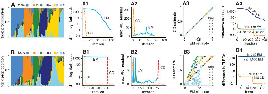
Figure 1: Results of fitting $K=6$ topic models to data sets A and B. Panels A and B show the topic proportions used to simulate the two data sets. Panels A1, A2, B1 and B2 show the improvement in the EM and CD estimates over time, as measured by the log-likelihood difference with respect to best $\log p_{\mathsf{topic}}({{\bf X}}\mid{\bf L}^{\star},{\bf F}^{\star})$ achieved among all fits, and by the maximum KKT residual. Plots A3 and B3 compare the final EM and CD estimates of the topic proportions. Panels A4 and B4 show the improvement in the LDA fit over time, in which VEM is initialized to the estimates obtained performing different numbers of EM and/or CD updates. Log-likelihood and ELBO differences less than 0.1 are shown as 0.1.

We ran the EM and CD algorithms on both data sets as described in Appendix A.6.3. We assessed convergence by examining the change in the log-likelihood and the residuals of the first-order Karush-Kuhn-Tucker (KKT) conditions; both should vanish near a solution. To reduce the possibility that different runs might find different local maxima of the likelihood, which could complicate the comparisons, we initialized the algorithms by running 50 EM updates. (By “update” or “iteration,” we mean one iteration of the outer loop in Algorithm 1.) Results are shown in Fig. 1.

In data set A, although CD converged faster, both algorithms progressed rapidly toward the same solution (Panels A1–A3). Thus, in this data set, use of EM or CD makes little practical difference. Data set B shows a different story. EM initially made good progress—in the initialization phase, which is not shown in the plots, the 50 EM updates improved the the log-likelihood by over 5,000—but after performing an 750 additional EM updates, the estimates remained far from the CD solution (Panels B1, B2). To be clear, EM continued to make progress even after 750 iterations, but this progress was slow; after the 750 iterations, the log-likelihood increased by about 0.1 at each iteration. Furthermore, the estimates of topic proportions differed substantially (Panel B3), showing that the large difference in likelihood reflects consequential differences in fit. In particular, EM often overestimated membership in topic 6, and consequently underestimated membership in other topics.

To rule out the possibility that EM had settled on a different local maximum, we performed an additional 200 CD updates from the final EM state (dashed, red line in Panels B1, B2). Doing so recovered the better CD solution. This illustrates the danger of the common, but incorrect, assumption that small changes in the objective imply proximity to a solution.

While the EM algorithm we use here performs ML estimation, similar “variational EM” (VEM) algorithms are frequently used to fit variational approximations for topic models, notably in LDA (Blei et al., 2003) in which point estimates $\hat{l}_{i1},\ldots,\hat{l}_{iK}$ are replaced by an estimated posterior, $\mathrm{Dirichlet}(\gamma_{i1},\ldots,\gamma_{iK})$. Given the similarity of the algorithms (Asuncion et al., 2009; Buntine and Jakulin, 2006; Faleiros and Lopes, 2016), one might expect VEM to have similar convergence issues to EM. To check this, we ran VEM for LDA, initializing $f_{jk}$ and $\gamma_{ik}$ using either the EM or CD estimates. To replicate the ML estimation setting as closely as possible, we used a fixed, uniform prior for the topic proportions. In both data sets, the CD initialization produced a better fit (higher “Evidence Lower Bound”, or ELBO) than the EM initializations (Panels A4 and B4). In data set B, the difference is particularly striking; the CD initialization produced a solution with ELBO that was over 1,000 units higher. These results suggest the potential for NMF methods to improve variational inference for LDA.

Note that the poor convergence of EM in data set B is not easily solved using existing acceleration schemes; the quasi-Newton-accelerated EM algorithm, implemented in the maptpx R package (Taddy, 2012), also converged slowly in this data set (Fig. A1).

5 NUMERICAL EXPERIMENTS

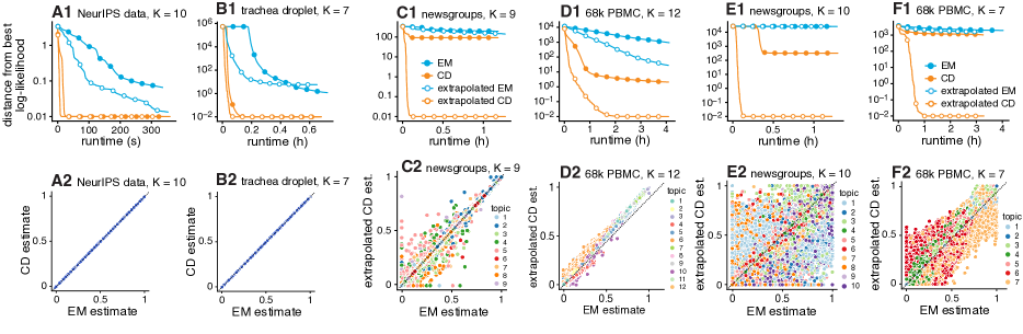
Figure 2: Selected results on fitting topic models using Poisson NMF algorithms. Panels A1 through F1 show the improvement in the topic model fit over time. (The 1,000 EM iterations performed during the initialization phase are not shown.) Log-likelihoods $\log p_{\mathsf{topic}}({{\bf X}}\mid{\bf L}^{\star},{\bf F}^{\star})$ are shown relative to the best log-likelihood obtained among the four algorithms compared. Log-likelihood differences less than 0.01 are shown as 0.01. Circles are plotted at every 100 iterations. Plots A2 though F2 compare final estimates of the topic proportions for all topics; in Plots C2 through F2, the proportions are coloured by topic. For extended results, see Figures A2–A9.

Having hinted at the advantages of CD over EM for fitting topic models, we now perform a more systematic comparison using real data sets. In particular, we compare Algorithm 1, implemented with EM or CD updates, with or without extrapolation (Ang and Gillis, 2019). We run these comparisons on four data sets (Table 1): two text data sets (Globerson et al., 2007; Rennie, 2007) that have been used to evaluate topic modeling methods (e.g., Asuncion et al. 2009; Wallach 2006); and two single-cell RNA sequencing (scRNA-seq) data sets (Montoro et al., 2018; Zheng et al., 2017). While the second application may be less familiar to readers, recent papers have illustrated the potential for topic models to uncover structure from scRNA-seq data, in particular structure that is not well captured by (hard) clustering (Dey et al., 2017; Xu et al., 2019; Bielecki et al., 2021; Hung et al., 2021). See Appendix A.6 for more details on the data.

Table 1: Data sets used in the experiments.

name	rows	columns	nonzeros
NeurIPS	2,483	14,036	3.7%
newsgroups	18,774	55,911	0.2%
trachea droplet	7,193	18,388	9.3%
68k PBMC	68,579	20,387	2.7%

To reduce the possibility that multiple optimizations converge to different local maxima of the likelihood, which could complicate the comparisons, we first ran 1,000 EM updates—that is, 1,000 iterations of the outer loop of Algorithm 1—then we examined the performance of the algorithms after this initialization phase. Therefore, in our comparisons we assessed the extent to which the different algorithms improve upon this initial fit. In addition to these quantitative performance comparisons, we also assessed whether different estimates qualitatively impact interpretation of the topics. The Appendix A.6 gives additional details on the experiment setup, and the supplement contains the source code used to generate the results presented here and in the Appendix.

In summary, our results showed that the extrapolated CD updates usually produced the best fit, and converged to a solution at least as fast as other algorithms, and often faster. Selected comparisons are shown in Fig. 2, with more comprehensive results (all four data sets, with $K$ ranging from 2 to 12) included in the Appendix (Figures A2–A9). The extrapolation consistently helped convergence of CD, and sometimes helped EM. The runtime per iteration was roughly the same in all algorithms (circles are plotted at every 100 iterations). Beyond these general patterns, there was considerable variation in the algorithms’ performance among the different data sets and within each data set at different settings of $K$. To make sense of the diverse results, we distinguish three main patterns.

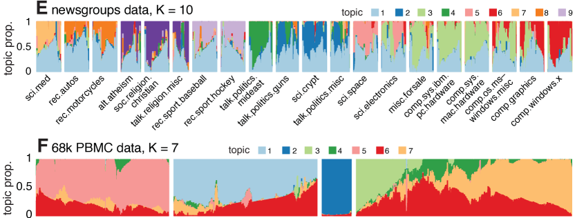
Figure 3: Extrapolated CD topic model fits visualized using Structure plots. Each bar represents a sample, and bar heights depict topic proportions. In Panel E, the documents are arranged by newsgroup. To create the Structure plot in Panel F, the cells are split into 4 clusters based on their topic proportions; the clusters, from left to right, contain 3733, 4028, 163 and 60,655 cells. To better visualize the smaller clusters in Panel F, larger clusters are subsampled in the plot.

Plots A1 and B1 in Fig. 2 illustrate the first pattern: EM achieved a reasonably good fit, so any improvements over EM were small regardless of the algorithm used. Indeed, the EM and CD estimates in these two examples are nearly indistinguishable (Fig. 2 A2, B2).

Plots C1 and D1 illustrate the second pattern: 1,000 iterations of EM was insufficient to obtain a good fit, and running additional EM or CD updates substantially improved the fit. Among the four algorithms, the extrapolated CD updates provided the greatest improvement. And yet the large difference in log-likelihood corresponded to only modest differences in estimated topic proportions (Plots C2, D2). So while the CD updates with extrapolation produced large gains in computational performance, these gains did not meaningfully impact the topic modeling results.

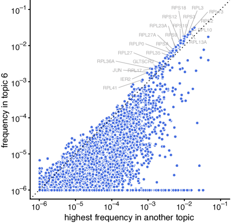
Figure A11: Gene frequencies in topic 6 vs. other topics in the multinomial topic model estimated from the 68k PBMC data using extrapolated CD updates, with $K=7$. Genes that have higher frequencies in topic 6 compared to other topics lie above the diagonal. Frequencies less than $10^{-6}$ are shown as $10^{-6}$.

Plots E1 and F1, showing results from the newsgroups and 68k PBMC data sets, are examples of the third pattern: the extrapolated CD updates outperformed the other updates, and produced estimated topic proportions strikingly different from the EM estimates (Plots E2, F2). To understand why, we examined the CD estimates of the topic proportions in Structure plots (Rosenberg, 2002) (Fig. 3). The topics with the greatest discrepancies between the EM and CD estimates are topic 1 in the newsgroups data and topics 3, 6 and 7 in the 68k PBMC data. Topic 1 in the newsgroups data and topic 6 in 68k PBMC data seem to capture global trends as they are present to some degree in most data samples. Topic 1 of the newsgroups is likely capturing “off-topic” discussion; none of the words appearing more frequently in topic 1 obviously point to any specific newsgroup (Fig. A10). In topic 6 of the 68k PBMC data, the genes with the largest expression increases are ribosomal protein genes (Fig. A11); abundance of ribosomal protein genes is known to be a major contributor to variation in PBMC scRNA-seq data sets (Freytag et al., 2018). Topics 3, 4, 6 and 7 capture heterogeneity in the largest cluster—the right-most cluster in Fig. 3F, mainly consisting of natural killer cells and T cells)—which brings to mind data set B in Sec. 4. By contrast, topics 1, 2 and 5, which identify myeloid cells, CD34+ cells and B cells, respectively, are mostly independent, and the EM and CD estimates for these topics do not differ much (Fig. 2, Panel F2). These results suggest that interdependent topics can impede EM’s convergence, and in these settings CD can offer large improvements.

6 DISCUSSION

We suggested a simple new strategy for fitting topic models by exploiting the equivalence of Poisson NMF and the multinomial topic model: first fit a Poisson NMF, then recover the corresponding topic model. To our knowledge this equivalence, despite being well appreciated, has not been previously exploited to fit topic models. This strategy worked best when Poisson NMF was optimized using a simple co-ordinate descent (CD) algorithm. While CD may be simple, consider that, due to the “sum-to-one” constraints, it is not obvious how to implement CD for the multinomial topic model.

It is a well known fact that EM can be slow to converge. Despite this, EM algorithms continue to be widely used to fit topic models, perhaps with the assumption that if the EM is run for a long time, the EM estimates will be “good enough.” We showed that this is sometimes not the case; EM updates producing a small change in the likelihood may still result in estimates with a much lower likelihood than—and may be very different from—the solution at a nearby fixed point. New models that improve on pLSI or LDA (e.g., Miao et al. 2016) therefore may partly reflect improvements in the optimization. There are of course many methods that improve convergence of EM, and some have had remarkable success. It would therefore be natural to apply these methods here. From experience however these methods provided only a modest improvement; maptpx (Fig. A1) was an example of this.

We focussed on ML estimation, but the ideas and algorithms presented here also apply to MAP estimation with Dirichlet priors on ${\bf F}^{\star}$. Extending these ideas to improve variational EM (VEM) for topic models (i.e., LDA) may also be of interest. As our examples demonstrate, simply initializing VEM from the solution found by our approach may already improve fits. However, given the success of the CD approach, it may also be fruitful to develop CD-based alternatives to VEM for Poisson NMF (Gopalan et al., 2015) That said, in many applications topic models are mainly used for dimension reduction—the goal being to learn compact representations of complex patterns—and in these applications, ML or MAP estimation may suffice.

Finally, some topic modeling applications involve massive data sets that require an “online” approach (Hoffman et al., 2010; Sato, 2001). Developing online versions of our algorithms is straightforward in principle, although online learning brings additional practical challenges, such as the choice of learning rates.

Acknowledgements

Many people have contributed ideas and feedback on this work, including Mihai Anitescu, Kushal Dey, Adam Gruenbaum, Anthony Hung, Youngseok Kim, Kaixuan Luo, John Novembre, Sebastian Pott, Alan Selewa and Jason Willwerscheid. We thank the staff at the Research Computing Center for providing the high-performance computing resources used to implement the numerical experiments. This work was supported by the NHGRI at the National Institutes of Health under award number 5R01HG002585.

Appendix A SUPPLEMENTARY MATERIALS

This supplement contains additional methods, results and discussion supporting the paper, “Non-negative matrix factorization algorithms greatly improve topic model fits,” including derivations of the EM algorithms (Sec. A.3); derivation of the KKT conditions for Poisson NMF (Sec. A.4); enhancements and implementation details for the Poisson NMF algorithms (Sec. A.5); details of the numerical experiments (Sec. A.6); and extended results of the numerical experiments (Sec. A.7).

A.1 Proof of Corollary 1

We prove Corollary 1 by contradiction. Suppose that $s_{i}\neq t_{i}$ for a given $i\in\{1,\ldots,n\}$, and in particular suppose that $s_{i}=a_{i}t_{i}$, where $a_{i}\neq 1$. From (4), we have $s_{i}=\sum_{k=1}^{K}l_{ik}u_{k}$. Then, propose new estimates $l_{ik}^{\prime}=l_{ik}/a_{i}$ for all $k=1,\ldots,K$, giving $s_{i}^{\prime}=\sum_{k=1}^{K}l_{ik}^{\prime}u_{k}=\sum_{k=1}^{K}l_{ik}u_{k}/a_{i}=a_{i}s_{i}=t_{i}$.

The topic proportions $l_{ik}^{\star}$ remain unchanged with these new estimates; that is $l_{ik}^{\star}=l_{ik}^{\prime}u_{k}/s_{i}^{\prime}=l_{ik}u_{k}/s_{i}$. (The word frequencies $f_{jk}^{\star}$ are trivially unchanged.) Therefore, substituting $s_{i}^{\prime}$ for $s_{i}$ does not change the topic model likelihood $p_{\mathsf{topic}}({\bf X}\mid{\bf L}^{\star},{\bf F}^{\star})$. However, $s_{i}^{\prime}=t_{i}$ is the MLE For $\mathrm{Poisson}(t_{i};s_{i})$, which means that the Poisson NMF likelihoood $p_{\mathsf{PNMF}}({\bf X}\mid{\bf L},{\bf F})$ can be improved by replacing $s_{i}$ with $s_{i}^{\prime}=t_{i}$. Therefore, estimates $s_{i}\neq t_{i}$ cannot be a Poisson NMF MLE.

The reverse direction is a straightforward application of Lemma 1 after setting $s_{i}=t_{i}$ for all $i=1,\ldots,n$.

A.2 Extension of Corollary 1 to MAP estimation

Corollary 2 (Relation between MAP estimates for Poisson NMF and multinomial topic model).

Let ${\hat{\bf L}}\in{\bf R}_{+}^{n\times K},\hat{\bf F}\in{\bf R}_{+}^{m\times K}$ denote maximum a posteriori (MAP) estimates for the Poisson NMF model, in which the elements of ${\bf F}$ are assigned independent gamma priors, $f_{jk}\sim\mathrm{Gamma}(\alpha_{jk},\beta_{k})$, with $\alpha_{jk}>1$ for all $j=1,\ldots,m$, $k=1,\ldots,K$, and ${\bf L}$ is assigned an (improper) uniform prior,

$$\hat{\bf L},\hat{\bf F}\in\underset{{\bf L},{\bf F}}{\mathrm{argmax}}\;p_{\mathsf{PNMF}}({\bf X}\mid{\bf L},{\bf F})\times\prod_{j=1}^{m}\prod_{k=1}^{K}\mathrm{Gamma}(f_{jk};\alpha_{jk},\beta_{k}),$$ (17)

where $\mathrm{Gamma}(\theta;\alpha,\beta)$ denotes the probability density of the gamma distribution with shape $\alpha$ and inverse scale $\beta$. If $\hat{{\bf L}}^{\star},\hat{{\bf F}}^{\star}$ are obtained by applying $\psi$ to $\hat{\bf L},\hat{\bf F}$, these will be MAP estimates for the multinomial topic model with independent Dirichlet priors on the columns of ${\bf F}$, $f_{1k},\ldots,f_{mk}\sim\mathrm{Dirichlet}(\alpha_{1k},\ldots,\alpha_{mk})$, and a uniform prior on ${\bf L}^{\star}$,

$$\hat{{\bf L}}^{\star},\hat{{\bf F}}^{\star}\in\underset{{\bf L}^{\star},{\bf F}^{\star}}{\mathrm{argmax}}\;p_{\mathsf{topic}}({\bf X}\mid{\bf L}^{\star},{\bf F}^{\star})\times\prod_{k=1}^{K}\mathrm{Dirichlet}(f_{1k},\ldots,f_{mk};\alpha_{1k},\ldots,\alpha_{mk}).$$ (18)

Conversely, let $\hat{{\bf L}}^{\star}\in{\bf R}_{+}^{n\times K},\hat{{\bf F}}^{\star}\in{\bf R}_{+}^{m\times K}$ denote MAP estimates for the multinomial topic model (18), set $s_{i}=t_{i}=\sum_{i=1}^{m}x_{ij}$, for $i=1,\dots,n$, and set $u_{k}=\sum_{j=1}^{m}(\alpha_{jk}-1)/\beta_{k}$, for $k=1,\dots,K$. Then if $\hat{{\bf L}},\hat{{\bf F}}$ are obtained by applying the inverse transformation $\psi^{-1}$ to $\hat{{\bf L}}^{\star},\hat{{\bf F}}^{\star},{\bm{s}},{\bm{u}}$, these will be MAP estimates for Poisson NMF (17).

A.3 EM algorithms

A.3.1 EM for the additive Poisson regression model

Here we derive the standard EM algorithm depierro-1993, appendix-lange-carson-1984, em-book, krishnan-1995, appendix-meng-1997, appendix-molina-2001, appendix-shepp-vardi-1982, appendix-vardi-1985 for fitting the additive Poisson regression model (9). First, we introduce latent variables $z_{ik}\sim\mathrm{Poisson}(a_{ik}b_{k})$ such that $\sum_{k=1}^{K}z_{ik}=y_{i}$, $i=1,\ldots,n$. Under the model augmented with the $z_{ik}$’s, the expected complete log-likelihood is

$$E[\log p({\bm{y}},{\bm{z}}\mid{\bf A},{\bm{b}})]=\sum_{i=1}^{n}\sum_{k=1}^{K}\phi_{ik}\log(a_{ik}b_{k})-\sum_{i=1}^{n}\sum_{k=1}^{K}a_{ik}b_{k}+\mbox{const},$$ (19)

where “const” includes additional terms in the likelihood that do not depend on ${\bm{b}}$, and $\bar{z}_{ik}=E[z_{ik}\mid{\bm{b}}]$ is the expectation of $z_{ik}$ with respect to the posterior $p({\bm{z}}\mid{\bf A},{\bm{b}})$. The M step (11) is derived by taking the partial derivative of (19) with respect to $b_{k}$, and solving for $b_{k}$. The E step involves computing posterior expectations at the current ${\bm{b}}=(b_{1},\ldots,b_{K})$. The posterior distribution of $z_{i}=(z_{i1},\ldots,z_{iK})$ is multinomial with $y_{i}$ trials and multinomial probabilities $p_{ik}\propto a_{ik}b_{k}$. Therefore, the posterior expected value of $z_{ik}$ is

$$\bar{z}_{ik}=y_{i}p_{ik}=y_{i}a_{ik}b_{k}/\mu_{i}.$$ (20)

The EM algorithm consists of iterating the E (10) and M (11) steps until some stopping criterion is met. Alternatively, the E and M steps can be combined, yielding the update

$$b_{k}^{\rm new}\leftarrow b_{k}\times\frac{\sum_{i=1}^{n}a_{ik}y_{i}/\mu_{i}}{\sum_{i=1}^{n}a_{ik}}.$$ (21)

A.3.2 EM for Poisson NMF

Here we derive an EM algorithm appendix-cemgil-2009, appendix-fevotte-2009 for Poisson NMF by applying the EM updates for the additive Poisson regression model that were derived in Appendix A.3.1. Making substitutions ${\bf A}\rightarrow{\bf F}$, ${\bm{y}}\rightarrow{\bm{x}}_{i}$, ${\bm{b}}\rightarrow{\bm{l}}_{i}$ in (21), where ${\bm{x}}_{i}$ is a row of ${{\bf X}}$ and ${\bm{l}}_{i}$ is a row of ${\bf L}$, and appropriately changing the indices, we arrive at the following update for the loadings:

$$l_{ik}^{\rm new}\leftarrow l_{ik}\times\frac{\sum_{j=1}^{m}x_{ij}f_{jk}/\lambda_{ij}}{\sum_{j=1}^{m}f_{jk}}$$ (22)

Similarly, making substitutions ${\bf A}\rightarrow{\bf L}$, ${\bm{y}}\rightarrow{\bm{x}}_{j}$, ${\bm{b}}\rightarrow{\bm{f}}_{j}$, where ${\bm{x}}_{j}$ is a column of ${{\bf X}}$ and ${\bm{f}}_{j}$ is a row of ${\bf F}$, the update for the factors is

$$f_{jk}^{\rm new}\leftarrow f_{jk}\times\frac{\sum_{i=1}^{n}x_{ij}l_{ik}/\lambda_{ij}}{\sum_{i=1}^{n}l_{ik}}.$$ (23)

These are the Poisson NMF “multiplicative” updates appendix-lee-seung-2001.

A.3.3 EM for the multinomial topic model

Here we derive EM for the multinomial topic model appendix-asuncion-2009, appendix-hofmann-2001, and draw a connection between EM for the multinomial topic model and the multiplicative updates for Poisson NMF.

The EM algorithm is based on the following augmented model appendix-blei-2003:

$$\begin{array}[]{r@{\;}c@{\;}l}p(z_{ir}=k\mid l_{i}^{\star})&=&l_{ik}^{\star}\\ p(w_{ir}=j\mid{\bf F}^{\star},z_{ir}=k)&=&f_{jk}^{\star},\end{array}$$ (24)

where we have introduced latent topic assignments $z_{ir}\in\{1,\ldots,K\}$, and the data are encoded as $w_{ir}\in\{1,\ldots,m\}$, for $r=1,\ldots,t_{i}$, with $t_{i}$ being the size of the $i$th document. Summing over the topic assignments $z_{ij}$, the augmented model (24) recovers the multinomial likelihood (3) up to a constant of proportionality; that is,

$$p({{\bf X}}\mid{\bf L}^{\star},{\bf F}^{\star})\propto{\textstyle\int p({\bm{w}},{\bm{z}}\mid{\bf L}^{\star},{\bf F}^{\star})\,d{\bm{z}}}\\ =\prod_{i=1}^{n}\prod_{r=1}^{t_{i}}\sum_{z_{ir}=1}^{K}p(w_{ir}\mid{\bf F}^{\star},z_{ir})\,p(z_{ir}\mid{\bm{l}}_{i}^{\star}),$$

in which the word counts in each document are recovered as $x_{ij}=\sum_{r=1}^{t_{i}}\delta_{j}(w_{ir})$

The E step consists of computing posterior expectations for the latent topic assignments $z_{ij}$,

$$p_{ijk} \equiv p(z_{ij}=k\mid{{\bf X}},{\bf L}^{\star},{\bf F}^{\star})=l_{ik}^{\star}f_{jk}^{\star}/\pi_{ij}.$$ (25)

The M step updates for the topic proportions $l_{ik}^{\star}$ and word frequencies $f_{jk}^{\star}$ are

$$l_{ik}^{\star} =\sum_{j=1}^{m}x_{ij}p_{ijk}/t_{i}$$ (26)

$$f_{jk}^{\star} \propto\sum_{i=1}^{n}x_{ij}p_{ijk}.$$ (27)

Combining the E (25) and M (26, 27) steps, we arrive at the following updates:

$$(l_{ik}^{\star})^{\rm new} \leftarrow\frac{l_{ik}^{\star}}{t_{i}}\sum_{j=1}^{m}x_{ij}f_{jk}^{\star}/\pi_{ij}$$ (28)

$$(f_{jk}^{\star})^{\rm new} \leftarrow\frac{f_{jk}^{\star}}{\xi_{k}}\sum_{i=1}^{n}x_{ij}l_{ik}^{\star}/\pi_{ij},$$ (29)

where $\xi_{k}$ is a normalizing constant ensuring that $(f_{1k}^{\star})^{\rm new}+\cdots+(f_{mk}^{\star})^{\rm new}=1$.

The same EM updates (28, 29) can also be derived in a different way, by applying the reparameterization (4) and its inverse to the Poisson NMF multiplicative updates (12, 13).

A.3.4 EM for the multinomial mixture model

The multinomial mixture model is

$$\begin{array}[]{r@{\;}c@{\;}l}y_{1},\ldots,y_{n}&\sim&\mathrm{Multinomial}(t,\pi_{1},\ldots,\pi_{n}),\\ \pi_{i}&=&a_{i1}^{\star}b_{1}^{\star}+\cdots+a_{iK}^{\star}b_{K}^{\star},\end{array}$$ (30)

in which the data are ${\bf A}^{\star}\in{\bf R}_{+}^{n\times K}$ and ${\bm{y}}=(y_{1},\ldots,y_{n})\in{\bf R}_{+}^{n}$, and $t=\sum_{i=1}^{n}y_{i}$. To ensure that the $\pi_{i}$’s are indeed probabilities, we require $b_{k}^{\star}\geq 0$, $a_{ik}^{\star}\geq 0$, $\sum_{k=1}^{K}b_{k}^{\star}=1$ and $\sum_{i=1}^{n}a_{ik}^{\star}=1$.

Omitting the derivation, the E and M steps for the multinomial mixture model (30) are

$$p_{ik} =\frac{a_{ik}^{\star}b_{k}^{\star}}{\sum_{k^{\prime}=1}^{K}a_{ik^{\prime}}^{\star}b_{k^{\prime}}^{\star}}$$ (31)

$$b_{k}^{\star} =\sum_{i=1}^{n}y_{i}p_{ik}/t.$$ (32)

A.3.5 Poisson regression–multinomial mixture model reparameterization

The additive Poisson regression model (9) is equivalent to the multinomial mixture model (30) by a simple reparameterization. For practical implementation (with finite precision arithmetic), the EM updates for the multinomial mixture model are more convenient, so we use the following reparameterization to implement EM for the additive Poisson regression model.

The multinomial mixture model (30) is a reparameterization of the Poisson regression model (9) that preserves the likelihood; that is,

$$\mathrm{Multinomial}({\bm{y}};t,\pi_{1},\ldots,\pi_{n})\times\mathrm{Poisson}(t;s)=\prod_{i=1}^{n}\mathrm{Poisson}(y_{i};\mu_{i}),$$ (33)

in which the parameters on the left-hand side are recovered from the parameters on the right-hand side as

$$\begin{array}[]{r@{\;}c@{\;}l}u_{k}&\leftarrow&a_{1k}+\cdots+a_{nk}\\ s&\leftarrow&b_{1}u_{1}+\cdots+b_{K}u_{K}\\ a_{ik}^{\star}&\leftarrow&a_{ik}/u_{k}\\ b_{k}^{\star}&\leftarrow&b_{k}u_{k}/s.\\ \end{array}$$ (34)

Once the multinomial parameters $b_{1}^{\star},\ldots,b_{K}^{\star}$ have been updated by performing one or more EM updates, the Poisson parameters $b_{1},\ldots,b_{K}$ are recovered as $b_{k}=tb_{k}^{\star}/u_{k}$ using the MLE of $s$, $\hat{s}=t$.

A.4 Derivation of KKT conditions for Poisson NMF optimization problem

Here we derive the first-order optimality (Karush-Kuhn-Tucker) conditions for the Poisson NMF optimization problem (7). The first-order KKT conditions for this optimization problem are

$$\nabla_{\bf F}\hat{\ell}({\bf L},{\bf F},{\bf\Gamma},{\bf\Omega}) =0$$ (35)

$$\nabla_{\bf L}\hat{\ell}({\bf L},{\bf F},{\bf\Gamma},{\bf\Omega}) =0$$ (36)

$${\bf\Omega}\odot{\bf F} =0$$ (37)

$${\bf\Gamma}\odot{\bf L} =0,$$ (38)

in which $\hat{\ell}({\bf L},{\bf F},{\bf\Gamma},{\bf\Omega})$ is the Lagrangian function,

$$\hat{\ell}({\bf L},{\bf F},{\bf\Gamma},{\bf\Omega})=\ell({\bf L},{\bf F})-\sum_{i=1}^{n}\sum_{k=1}^{K}\gamma_{ik}l_{ik}-\sum_{j=1}^{m}\sum_{k=1}^{K}\omega_{jk}f_{jk}.$$ (39)

Here we have introduced matrices of Lagrange multipliers ${\bf\Gamma}\in{\bf R}_{+}^{n\times K}$ and ${\bf\Omega}\in{\bf R}_{+}^{m\times K}$ associated with the non-negativity constraints ${\bf L}\geq 0$ and ${\bf F}\geq 0$. Combining conditions (35) and (36), we obtain

$${\bf\Omega} =(1-{\bf U})^{T}{\bf L}$$ (40)

$${\bf\Gamma} =(1-{\bf U}){\bf F},$$ (41)

in which ${\bf U}\in{\bf R}_{+}^{n\times m}$ with entries $u_{ij}=x_{ij}/({\bf L}{\bf F}^{T})_{ij}$. See appendix-dhillon-2005 and appendix-fevotte-2011 for generalizations of these conditions.

A.5 Additional enhancements and implementation details

Here we describe additional enhancements to the Poisson NMF algorithms and other implementation details.

To obtain a good initialization of ${\bf L}$ and ${\bf F}$, we used the Topic-SCORE algorithm ke-2019 to estimate ${\bf F}$, then we performed 10 CD updates of ${\bf L}$. We found that the Topic-SCORE algorithm was very fast, and typically completed in less time than it took to run a single outer-loop iteration in Algorithm 1).

Following common practice in co-ordinate descent algorithms, we incompletely solved each subproblem $\text{\sc fit-pois-reg}({\bf L},{\bm{x}}_{j})$ and $\text{\sc fit-pois-reg}({\bf F},{\bm{x}}_{i})$; the intuition is that accurately solving each subproblem is wasted effort, particularly early on when the estimates change a lot from one iteration to the next. We found that 4 EM or 4 CD updates worked well when initialized to the estimate obtained in the previous (outer loop) iteration. Incompletely solving the subproblems has been similarly shown to work well for Frobenius-norm NMF gillis-2012, appendix-ccd, appendix-kim-2014.

Whenever we used CD to optimize $\text{\sc fit-pois-reg}({\bf A},{\bm{y}})$, we performed a single EM update prior to running the CD updates. This nudged the estimate closer to the solution, and improved convergence of CD (in the absence of a line search).

To help with convergence of the updates to ${\bf L}$ and ${\bf F}$, any updated parameters that fell below $10^{-15}$ were set to this value. This step was motivated by Theorem 1 of gillis-2012.

To improve numerical stability of the updates, as others have done (e.g., appendix-lee-seung-1999), we rescaled ${\bf F}$ and ${\bf L}$ after each full update. Specifically, we rescaled the matrices so that the column means of ${\bf F}$ were equal to the column means of ${\bf L}$. Note that the Poisson rates $\lambda_{ij}=({\bf L}{\bf F}^{T})_{ij}$ and the likelihood $p_{\sf PNMF}({{\bf X}}\mid{\bf L},{\bf F})$ are invariant to this rescaling.

We used Intel Threading Building Blocks (TBB) multithreading to optimize the $\text{\sc fit-pois-reg}({\bf F},{\bm{x}}_{i})$ and $\text{\sc fit-pois-reg}({\bf L},{\bm{x}}_{j})$ subproblems in parallel. We also used sparse matrix computation techniques to leverage sparsity of the count data. This latter substantially reduced computation for all data sets, which displayed high levels of sparsity (¿90% of entries equal to zero). For sparse ${\bf X}$, the complexity of computing the Poisson NMF likelihood, for example, is $O((N+n+m)K)$, where $N$ is the number of nonzeros in ${\bf X}$, whereas for non-sparse ${\bf X}$ the complexity is $O(nmK)$.

Finally, we used two measures to assess the quality of the computed solutions to (7): the change in the loss function $\ell({\bf L},{\bf F})$ or, equivalently, the change in the Poisson NMF log-likelihood, $\log p_{\sf PNMF}({\bf X}\mid{\bf L},{\bf F})$; and the maximum residual of the KKT conditions (40, 41).

A.6 Details of numerical experiments

These sections give additional details on preparation of the data sets (Sec. A.6.1), the computing setup (Sec. A.6.2), and software and code used (Sec. A.6.3) for the numerical experiments (Sec. 5).

A.6.1 Data sets

See Table 1 for summary of data sets used in the numerical experiments. The NeurIPS appendix-globerson-2007 and newsgroups appendix-newsgroups data sets are word counts extracted from, respectively, 1988–2003 NeurIPS (formerly NIPS) papers and posts to 20 different newsgroups. Both data sets have been used to evaluate topic modeling methods (e.g., appendix-asuncion-2009, appendix-wallach-2006). The trachea droplet appendix-montoro-2018 and 68k PBMC appendix-zheng-2017 data are UMI (unique molecular identifier) counts from droplet-based single-cell RNA sequencing experiments in trachea epithelial cells in C57BL/6 mice and in “unsorted” human peripheral blood mononuclear cells (PBMCs) [Fresh 68k PBMC Donor A], processed using the GemCode Single Cell Platform. The 68k PBMC data have been used to benchmark methods for single-cell RNA-seq data (e.g., abdelaal-2019, diaz-mejia-2019, townes-2019). The data sets were retrieved from http://ai.stanford.edu/~gal/data.html (NeurIPS), http://qwone.com/~jason/20Newsgroups (newsgroups), https://support.10xgenomics.com/single-cell-gene-expression/datasets (68k PBMC), and the Gene Expression Omnibus (GEO), accession GSE103354 (trachea droplet).

The trachea droplet data are publicly available on the GEO website and as such follow the NCBI copyright and data usage policies (https://www.ncbi.nlm.nih.gov/home/about/policies); see also https://www.ncbi.nlm.nih.gov/geo/info/disclaimer.html for GEO data disclaimers. The 68k PBMC data are distributed under the CC BY 4.0 license. The 68k PBMC and trachea droplet data were obtained under IRB-approved protocols; see appendix-montoro-2018, appendix-zheng-2017 for details. The NeurIPS and newsgroups data sets are distributed without a license.

All data sets were stored as sparse $n\times m$ count matrices ${\bf X}$, where $n$ is the number of documents or cells, and $m$ is the number of words or genes. The scripts used to prepare the data from the source files and the prepared NeurIPS and newsgroups data sets are provided in the supplementary materials.

A.6.2 Computing environment

All computations on real data sets were run in R 3.5.1 R, linked to the OpenBLAS 0.2.19 optimized numerical libraries, on Linux machines (Scientific Linux 7.4) with Intel Xeon E5-2680v4 (“Broadwell”) processors. For performing the Poisson NMF optimization, which includes some multithreaded computations, 8 CPUs and 16 GB of memory were used.

A.6.3 Source code and software

The methods were implemented in the fastTopics R package (the results were generated using version 0.5-24 of the package). The core optimization algorithms were developed in C++ and interfaced to R using Rcpp rcpp. The CD updates were adapted from the C++ code included with R package NNLM 0.4-3 nnlm. For the maptpx results, we used a slightly modified version of the maptpx package (version 1.9-8), available at https://github.com/stephenslab/maptpx, that allows initialization of both the topic proportions as well as the word frequencies. For the variational EM results, we used the C implementation by Blei et al (http://www.cs.columbia.edu/~blei/lda-c), which was interfaced to R using the topicmodels package topicmodels. The git repository https://github.com/stephenslab/fastTopics-experiments contains code implementing the numerical experiments, and a workflowr website workflowr for browsing the results.

A.7 Extended results

Figure A1 shows the results from running maptpx on the two simulated data sets (Sec. 4). Figures A2–A9 give more detailed results on the Poisson NMF algorithms’ progress in fitting topic models to the real data sets (Sec. 5). The scatterplots in Figures A10 and A11 highlight words and genes that appear more frequently in one topic compared to the other topics.

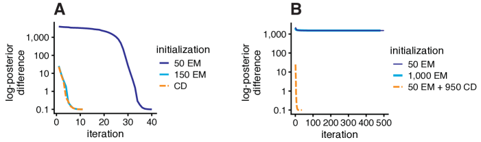
Figure A1: Maximum a posteriori (MAP) estimation of the multinomial topic model parameters, with $K=6$, using the quasi-Newton-accelerated EM algorithm implemented in maptpx appendix-taddy-2012. Plots A and B shows the improvement in the log-posterior over time in Scenarios A and B, in which the MAP estimates are initialized to MLEs obtained by performing different numbers of EM and/or CD updates.

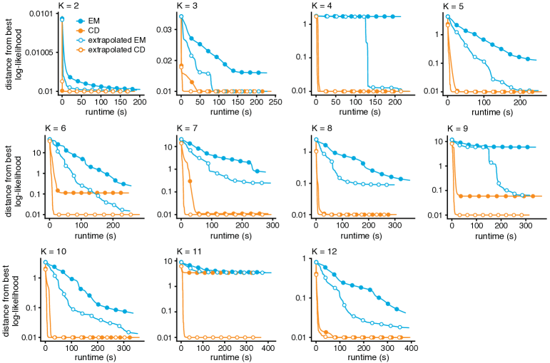
Figure A2: Improvement in model fit over time for the Poisson NMF algorithms applied to the NeurIPS data, with $K=2,\ldots,12$. Multinomial topic model log-likelihoods $\log p_{\mathsf{topic}}({{\bf X}}\mid{\bf L}^{\star},{\bf F}^{\star})$ are shown relative to the best log-likelihood recovered among the four algorithms compared (EM and CD, with and without extrapolation). The 1,000 EM iterations performed during the initialization phase are not shown. Log-likelihood differences less than 0.01 are shown as 0.01. Circles are drawn at intervals of 100 iterations.

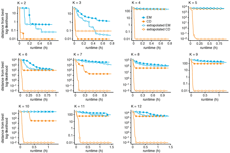
Figure A3: Improvement in model fit over time for the Poisson NMF algorithms applied to the newsgroups data, with $K=2,\ldots,12$. See the Fig. A2 caption for details.

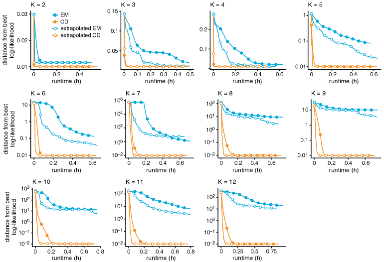
Figure A4: Improvement in model fit over time for the Poisson NMF algorithms applied to the trachea droplet data, with $K=2,\ldots,12$. See the Fig. A2 caption for details.

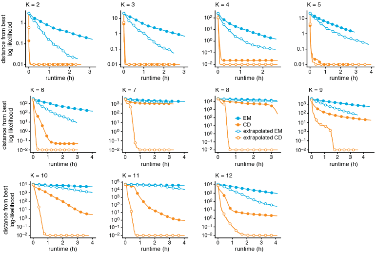
Figure A5: Improvement in model fit over time for the Poisson NMF algorithms applied to the 68k PBMC data, with $K=2,\ldots,12$. See the Fig. A2 caption for details.

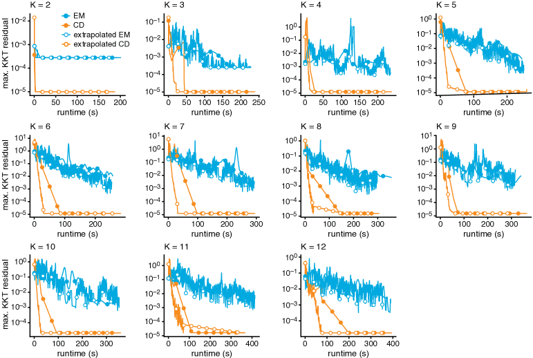
Figure A6: Evolution of the KKT residuals over time for the Poisson NMF algorithms applied to the NeurIPS data, with $K=2,\ldots,12$. The KKT residuals should vanish near a local maximum of the likelihood, so looking at the largest KKT residual can be used to assess how well the algorithm recovers an MLE. Note that, unlike the likelihood, the KKT residuals are not expected to decrease monotonically over time. Circles are drawn at intervals of 100 iterations.

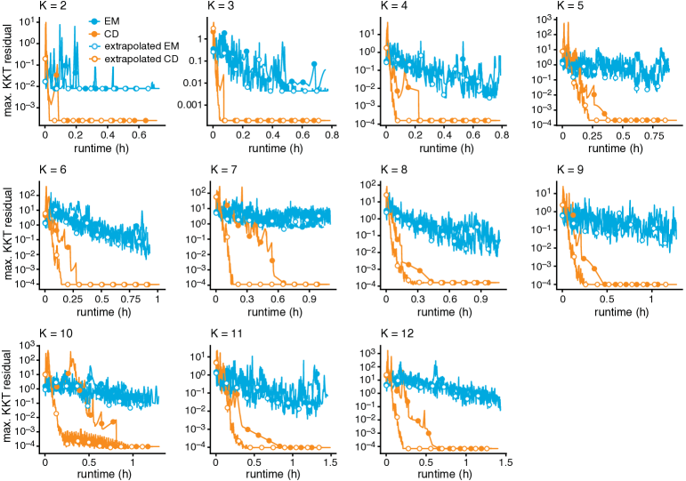
Figure A7: Evolution of the KKT residuals over time for the Poisson NMF algorithms applied to the newsgroups data, with $K=2,\ldots,12$. See the Fig. A6 caption for details.

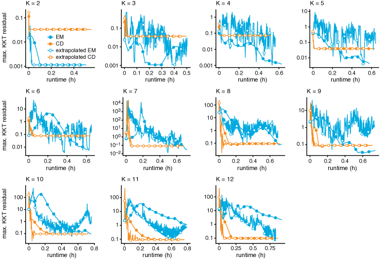
Figure A8: Evolution of the KKT residuals over time for the Poisson NMF algorithms applied to the trachea droplet data, with $K=2,\ldots,12$.

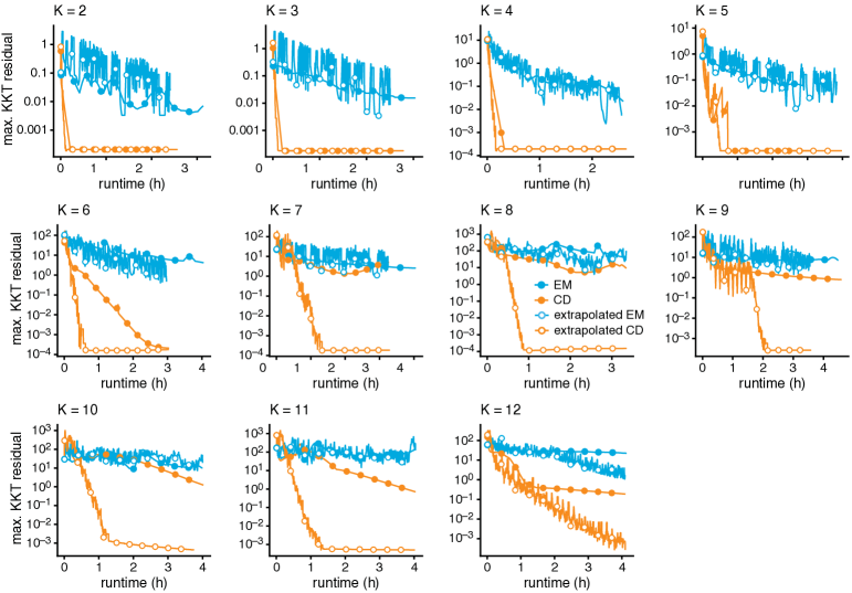
Figure A9: Evolution of the KKT residuals over time for the Poisson NMF algorithms applied to the 68k PBMC data, with $K=2,\ldots,12$.

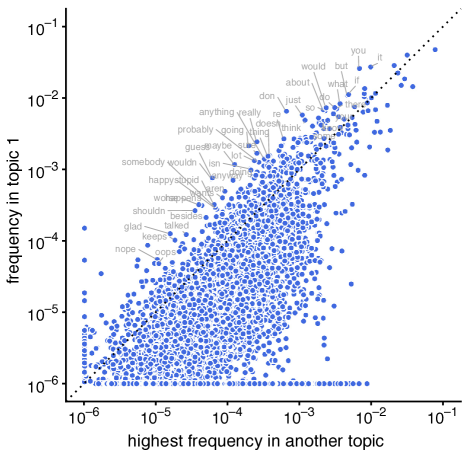
Figure A10: Word frequencies in topic 1 vs. other topics in the multinomial topic model estimated from the newsgroups data using extrapolated CD updates, with $K=10$. Words that are more frequent in topic 1 compared to other topics lie above the diagonal. Frequencies less than $10^{-6}$ are shown as $10^{-6}$.

abbrvnat fastTopics

References

- Aitchison (1982) J. Aitchison. The statistical analysis of compositional data. Journal of the Royal Statistical Society, Series B, 44(2):139–160, 1982.
- Ang and Gillis (2019) A. M. S. Ang and N. Gillis. Accelerating nonnegative matrix factorization algorithms using extrapolation. Neural Computation, 31(2):417–439, 2019.
- Asuncion et al. (2009) A. Asuncion, M. Welling, P. Smyth, and Y. W. Teh. On smoothing and inference for topic models. In Proceedings of the 25th Conference on Uncertainty in Artificial Intelligence, pages 27–34, 2009.
- Bertsekas (1999) D. P. Bertsekas. Nonlinear programming. Athena Scientific, Belmont, MA, 2nd edition, 1999.
- Bielecki et al. (2021) P. Bielecki, S. J. Riesenfeld, J.-C. Hütter, E. Torlai Triglia, M. S. Kowalczyk, R. R. Ricardo-Gonzalez, M. Lian, M. C. Amezcua Vesely, L. Kroehling, H. Xu, M. Slyper, C. Muus, L. S. Ludwig, E. Christian, L. Tao, A. J. Kedaigle, H. R. Steach, A. G. York, M. H. Skadow, P. Yaghoubi, D. Dionne, A. Jarret, H. M. McGee, C. B. M. Porter, P. Licona-Limón, W. Bailis, R. Jackson, N. Gagliani, G. Gasteiger, R. M. Locksley, A. Regev, and R. A. Flavell. Skin-resident innate lymphoid cells converge on a pathogenic effector state. Nature, 592:128–132, 2021.
- Blei and Lafferty (2007) D. M. Blei and J. D. Lafferty. A correlated topic model of Science. Annals of Applied Statistics, 1(1):17–35, 2007.
- Blei et al. (2003) D. M. Blei, A. Y. Ng, and M. I. Jordan. Latent Dirichlet allocation. Journal of Machine Learning Research, 3:993–1022, 2003.
- Bouman and Sauer (1996) C. Bouman and K. Sauer. A unified approach to statistical tomography using coordinate descent optimization. IEEE Transactions on Image Processing, 5(3):480–492, 1996.
- Buntine (2002) W. Buntine. Variational extensions to EM and multinomial PCA. In Proceedings of the 13th European Conference on Machine Learning, pages 23–34, 2002.
- Buntine and Jakulin (2006) W. Buntine and A. Jakulin. Discrete component analysis. In M. Saunders, Craigand Grobelnik, S. Gunn, and J. Shawe-Taylor, editors, Subspace, latent structure and feature selection, pages 1–33, Berlin, Heidelberg, 2006. Springer.
- Canny (2004) J. Canny. GaP: a factor model for discrete data. In Proceedings of the 27th Annual International ACM SIGIR Conference, pages 122–129, 2004.
- Cemgil (2009) A. T. Cemgil. Bayesian inference for nonnegative matrix factorisation models. Computational Intelligence and Neuroscience, 2009:785152, 2009.
- Cichocki et al. (2011) A. Cichocki, S. Cruces, and S.-I. Amari. Generalized alpha-beta divergences and their application to robust nonnegative matrix factorization. Entropy, 13(1):134–170, 2011.
- Cohen and Rothblum (1993) J. E. Cohen and U. G. Rothblum. Nonnegative ranks, decompositions, and factorizations of nonnegative matrices. Linear Algebra and its Applications, 190(1977):149–168, 1993.
- Dempster et al. (1977) A. P. Dempster, N. M. Laird, and D. B. Rubin. Maximum likelihood from incomplete data via the EM algorithm. Journal of the Royal Statistical Society, Series B, 39:1–22, 1977.
- Dey et al. (2017) K. K. Dey, C. J. Hsiao, and M. Stephens. Visualizing the structure of RNA-seq expression data using grade of membership models. PLoS Genetics, 13(3):e1006599, 2017.
- Dhillon and Sra (2005) I. S. Dhillon and S. Sra. Generalized nonnegative matrix approximations with Bregman divergences. In Advances in Neural Information Processing Systems, volume 18, pages 283–290, 2005.
- Ding et al. (2008) C. Ding, T. Li, and W. Peng. On the equivalence between non-negative matrix factorization and probabilistic latent semantic indexing. Computational Statistics and Data Analysis, 52(8):3913–3927, 2008.
- Faleiros and Lopes (2016) T. Faleiros and A. Lopes. On the equivalence between algorithms for non-negative matrix factorization and latent Dirichlet allocation. In Proceedings of the 24th European Symposium on Artificial Neural Networks, pages 171–176, 2016.
- Févotte and Idier (2011) C. Févotte and J. Idier. Algorithms for nonnegative matrix factorization with the -divergence. Neural Computation, 23(9):2421–2456, 2011.
- Fisher (1922) R. A. Fisher. On the interpretation of from contingency tables, and the calculation of P. Journal of the Royal Statistical Society, 85(1):87–94, 1922.
- Freytag et al. (2018) S. Freytag, L. Tian, I. Lönnstedt, M. Ng, and M. Bahlo. Comparison of clustering tools in R for medium-sized 10x genomics single-cell RNA-sequencing data. F1000Research, 7:1297, 2018.
- Gaussier and Goutte (2005) E. Gaussier and C. Goutte. Relation between PLSA and NMF and implications. In Proceedings of the 28th Annual International ACM SIGIR Conference, pages 601–602, 2005.
- Gillis (2014) N. Gillis. The why and how of nonnegative matrix factorization. arXiv, 1401.5226, 2014.
- Gillis (2021) N. Gillis. Nonnegative matrix factorization. Society for Industrial and Applied Mathematics, Philadelphia, PA, 2021.
- Globerson et al. (2007) A. Globerson, G. Chechik, F. Pereira, and N. Tishby. Euclidean embedding of co-occurrence data. Journal of Machine Learning Research, 8:2265–2295, 2007.
- González-Blas et al. (2019) C. González-Blas, L. Minnoye, D. Papasokrati, S. Aibar, G. Hulselmans, V. Christiaens, K. Davie, J. Wouters, and S. Aerts. cisTopic: cis-regulatory topic modeling on single-cell ATAC-seq data. Nature Methods, 16(5):397–400, 2019.
- Good (1986) I. J. Good. Some statistical applications of Poisson’s work. Statistical Science, 1(2):157–170, 1986.
- Gopalan et al. (2015) P. Gopalan, J. M. Hofman, and D. M. Blei. Scalable recommendation with hierarchical Poisson factorization. In Proceedings of the 31st Conference on Uncertainty in Artificial Intelligence, pages 326–335, 2015.
- Griffiths and Steyvers (2004) T. L. Griffiths and M. Steyvers. Finding scientific topics. Proceedings of the National Academy of Sciences, 101(Supplement 1):5228–5235, 2004.
- Henderson and Varadhan (2019) N. C. Henderson and R. Varadhan. Damped Anderson acceleration with restarts and monotonicity control for accelerating EM and EM-like algorithms. Journal of Computational and Graphical Statistics, 28(4):834–846, 2019.
- Hien and Gillis (2021) L. T. K. Hien and N. Gillis. Algorithms for nonnegative matrix factorization with the Kullback–Leibler divergence. Journal of Scientific Computing, 87(3):93, 2021.
- Hoffman et al. (2010) M. Hoffman, F. Bach, and D. Blei. Online learning for latent Dirichlet allocation. In Advances in Neural Information Processing Systems, volume 23, pages 856–864, 2010.
- Hofmann (1999) T. Hofmann. Probabilistic latent semantic indexing. In Proceedings of the 22nd Annual International ACM SIGIR Conference, pages 50–57, 1999.
- Hofmann (2001) T. Hofmann. Unsupervised learning by probabilistic latent semantic analysis. Machine Learning, 42(1):177–196, 2001.
- Hofmann et al. (1999) T. Hofmann, J. Puzicha, and M. Jordan. Learning from dyadic data. In Advances in Neural Information Processing Systems, volume 11, pages 466–472, 1999.
- Hsieh and Dhillon (2011) C.-J. Hsieh and I. S. Dhillon. Fast coordinate descent methods with variable selection for non-negative matrix factorization. In Proceedings of the 17th ACM SIGKDD International Conference, pages 1064–1072, 2011.
- Hung et al. (2021) A. Hung, G. Housman, E. A. Briscoe, C. Cuevas, and Y. Gilad. Characterizing gene expression responses to biomechanical strain in an in vitro model of osteoarthritis. bioRxiv, 2021. doi: 10.1101/2021.02.22.432314.
- Kim et al. (2014) J. Kim, Y. He, and H. Park. Algorithms for nonnegative matrix and tensor factorizations: a unified view based on block coordinate descent framework. Journal of Global Optimization, 58(2):285–319, 2014.
- Lange and Carson (1984) K. Lange and R. Carson. EM reconstruction algorithms for emission and transmission tomography. Journal of Computer Assisted Tomography, 8(2):306–316, 1984.
- Lee and Seung (1999) D. D. Lee and H. S. Seung. Learning the parts of objects by non-negative matrix factorization. Nature, 401(6755):788–791, 1999.
- Lee and Seung (2001) D. D. Lee and H. S. Seung. Algorithms for non-negative matrix factorization. In Advances in Neural Information Processing Systems, volume 13, pages 556–562, 2001.
- Lin and Boutros (2020) X. Lin and P. C. Boutros. Optimization and expansion of non-negative matrix factorization. BMC Bioinformatics, 21:7, 2020.
- Lucy (1974) L. Lucy. An iterative algorithm for the rectification of observed distributions. The Astronomical Journal, 79:745–754, 1974.
- Luenberger and Ye (2015) D. G. Luenberger and Y. Ye. Linear and nonlinear programming. Springer, 4th edition, 2015.
- McCullagh (1989) P. McCullagh. Generalized linear models. Chapman and Hall, New York, 2nd edition, 1989.
- Meng and Van Dyk (1997) X.-L. Meng and D. Van Dyk. The EM algorithm—an old folk-song sung to a fast new tune. Journal of the Royal Statistical Society, Series B, 59(3):511–567, 1997.
- Miao et al. (2016) Y. Miao, L. Yu, and P. Blunsom. Neural variational inference for text processing. In Proceedings of The 33rd International Conference on Machine Learning, pages 1727–1736, 2016.
- Minka and Lafferty (2002) T. Minka and J. Lafferty. Expectation propagation for the generative aspect model. In Proceedings of the 18th Conference on Uncertainty in Artificial Intelligence, pages 352–359, 2002.
- Montoro et al. (2018) D. T. Montoro, A. L. Haber, M. Biton, V. Vinarsky, B. Lin, S. E. Birket, F. Yuan, S. Chen, H. M. Leung, J. Villoria, N. Rogel, G. Burgin, A. M. Tsankov, A. Waghray, M. Slyper, J. Waldman, L. Nguyen, D. Dionne, O. Rozenblatt-Rosen, P. R. Tata, H. Mou, M. Shivaraju, H. Bihler, M. Mense, G. J. Tearney, S. M. Rowe, J. F. Engelhardt, A. Regev, and J. Rajagopal. A revised airway epithelial hierarchy includes CFTR-expressing ionocytes. Nature, 560(7718):319–324, 2018.
- Nocedal and Wright (2006) J. Nocedal and S. J. Wright. Numerical optimization. Springer, New York, NY, 2nd edition, 2006.
- Rennie (2007) J. Rennie. 20 newsgroups data set, 2007. URL http://qwone.com/~jason/20Newsgroups.
- Richardson (1972) W. H. Richardson. Bayesian-based iterative method of image restoration. Journal of the Optical Society of America, 62(1):55–59, 1972.
- Rosenberg (2002) N. A. Rosenberg. Genetic structure of human populations. Science, 298(5602):2381–2385, 2002.
- Sato (2001) M.-A. Sato. Online model selection based on the variational Bayes. Neural Computation, 13(7):1649–1681, 2001.
- Shepp and Vardi (1982) L. A. Shepp and Y. Vardi. Maximum likelihood reconstruction for emission tomography. IEEE Transactions on Medical Imaging, 1(2):113–122, 1982.
- Singh and Gordon (2008) A. P. Singh and G. J. Gordon. A unified view of matrix factorization models. In Joint European Conference on Machine Learning and Knowledge Discovery in Databases, volume 2, pages 358–373, 2008.
- Steyvers and Griffiths (2006) M. Steyvers and T. Griffiths. Probabilistic topic models. In T. landauer, D. McNamara, S. Dennis, and W. Kintsch, editors, Latent semantic analysis: a road to meaning, pages 427–448. Lawrence Erlbaum, 2006.
- Taddy (2012) M. Taddy. On estimation and selection for topic models. In N. D. Lawrence and M. Girolami, editors, Proceedings of the 15th International Conference on Artificial Intelligence and Statistics, volume 22, pages 1184–1193, La Palma, Canary Islands, 2012. PMLR.
- Teh et al. (2007) Y. W. Teh, D. Newman, and M. Welling. A collapsed variational Bayesian inference algorithm for latent Dirichlet allocation. In Advances in Neural Information Processing Systems, volume 19, pages 1353–1360, 2007.
- Vardi et al. (1985) Y. Vardi, L. A. Shepp, and L. Kaufman. A statistical model for positron emission tomography. Journal of the American Statistical Association, 80(389):8–20, 1985.
- Wallach (2006) H. M. Wallach. Topic modeling: beyond bag-of-words. In Proceedings of the 23rd International Conference on Machine Learning, pages 977–984, 2006.
- Wright (2015) S. J. Wright. Coordinate descent algorithms. Mathematical Programming, 151:3–34, 2015.
- Xu et al. (2019) H. Xu, J. Ding, C. B. Porter, A. Wallrapp, M. Tabaka, S. Ma, S. Fu, X. Guo, S. J. Riesenfeld, C. Su, D. Dionne, L. T. Nguyen, A. Lefkovith, O. Ashenberg, P. R. Burkett, H. N. Shi, O. Rozenblatt-Rosen, D. B. Graham, V. K. Kuchroo, A. Regev, and R. J. Xavier. Transcriptional atlas of intestinal immune cells reveals that neuropeptide -CGRP modulates group 2 innate lymphoid cell responses. Immunity, 51(4):696–708, 2019.
- Zheng et al. (2017) G. X. Y. Zheng, J. M. Terry, P. Belgrader, P. Ryvkin, Z. W. Bent, R. Wilson, S. B. Ziraldo, T. D. Wheeler, G. P. McDermott, J. Zhu, M. T. Gregory, J. Shuga, L. Montesclaros, J. G. Underwood, D. A. Masquelier, S. Y. Nishimura, M. Schnall-Levin, P. W. Wyatt, C. M. Hindson, R. Bharadwaj, A. Wong, K. D. Ness, L. W. Beppu, H. J. Deeg, C. McFarland, K. R. Loeb, W. J. Valente, N. G. Ericson, E. A. Stevens, J. P. Radich, T. S. Mikkelsen, B. J. Hindson, and J. H. Bielas. Massively parallel digital transcriptional profiling of single cells. Nature Communications, 8:14049, 2017.
- Zhou et al. (2011) H. Zhou, D. Alexander, and K. Lange. A quasi-Newton acceleration for high-dimensional optimization algorithms. Statistics and Computing, 21(2):261–273, 2011.
- Zhou et al. (2012) M. Zhou, L. Hannah, D. Dunson, and L. Carin. Beta-negative binomial process and Poisson factor analysis. In Proceedings of the 15th International Conference on Artificial Intelligence and Statistics, pages 1462–1471, 2012.