Stochastic resonance and amplification in the ac driven Duffing oscillator with added noise

Abstract

Stochastic resonance (SR) is a coherence enhancement effect due to noise that occurs in periodically-driven nonlinear dynamical systems. A very broad range of physical and biological systems present this effect such as climate change, neurons, neural networks, lasers, SQUIDS, and tunnel diodes, among many others. Early theoretical models of SR dealt only with overdamped bistable oscillators. Here, we propose a simple model that accounts for SR in an underdamped driven Duffing oscillator with added white noise. Furthermore, we develop a theoretical method to predict the effect of white noise on the pump, signal, and idler responses of a Duffing amplifier. We also calculate the power spectral density of the response of the Duffing amplifier. This approach may prove to be useful for assessing the robustness of acoustic, phononic, or mechanical frequency-comb generation to the presence of noise.

I Introduction

Stochastic resonance (SR) is a coherence enhancement effect caused by noise that occurs in periodically-driven nonlinear dynamical systems. The hallmark feature of this effect is characterized by the resonant behavior of the signal-to-noise ratio as a function of the noise level. A very broad range of physical and biological systems present this effect such as climate change Benzi et al. (1981), neurons Longtin (1993), neural networks Ikemoto et al. (2018), lasers McNamara et al. (1988), SQUIDS Hibbs et al. (1995), tunnel diodes Mantegna and Spagnolo (1994), nanomechanical oscillators Badzey and Mohanty (2005), etc.

Just a few years after the discovery of SR, in the mid 80’s, Jeffries and Wiesenfeld started studying the effect of small signals on non-autonomous nonlinear dynamical systems near bifurcation points Jeffries and Wiesenfeld (1985); Wiesenfeld (1985). They showed that several different systems are very sensitive to noise and coherent perturbations near the onset of codimention-one bifurcations, such as period doubling, saddle node, transcritical, Hopf, and pitchfork (symmetry-breaking) bifurcations. Initially, the effect of broadband noise was investigated (theoretically and experimentally) near period-doubling and Hopf bifurcations in a periodically driven $p$-$n$ junction . They found precursors of the bifurcations, such as new lines in the power spectrum, as the noise level was increased. Later on, a general theoretical framework, based on perturbation and Floquet theories, explaining the effects of small coherent signals perturbing nonlinear systems near the onset of bifurcation points was developed Wiesenfeld and McNamara (1985, 1986), with applications to the ac-driven Duffing oscillator. It was found that nonlinear dynamical systems could be used as narrow-band phase sensitive amplifiers.

With the advent and development of MEMS technology in the 90’s, new mechanical resonators were developed, such as the doubly-clamped beam resonators that could reach very high quality factors. The dynamics of the fundamental mode of these resonators is well approximated by the Duffing equation. Furthermore, these micromechanical devices exhibit a bistable response that can be quantitatively modelled by Duffing oscillators Aldridge and Cleland (2005). Nanomechanical resonators were implemented experimentally that use bifurcation points and SR as a very sensitive means of amplification R. Almog, S. Zaitsev, O. Shtempluck, and Buks (2007). Another method of amplification of small signals with a driven Duffing oscillator with added noise was recently proposed by Ochs et al. Ochs et al. (2021).

Early theoretical models of SR McNamara and Wiesenfeld (1989); Dykman et al. (1995); Gammaitoni et al. (1998) dealt only with overdamped bistable oscillators, neglecting altogether inertia terms in the dynamics. Although other methods have been proposed to explain SR behavior in underdamped oscillators, such as the method of moments Alfonsi et al. (2000); Kang et al. (2003); Landa et al. (2008), in which a Fokker-Planck equation model was used, the theory is considerably more complex than the model we propose here. Stocks et al. Stocks et al. (1993) proposed a model for SR in an underdamped monostable Duffing oscillator based on susceptibility calculations obtained directly from the fluctuation-dissipation theorem Landau and Lifshitz (1980) and the noise spectral density given in Dykman et al. (1990). When these pieces of the theory are combined the model becomes complex as well. Furthermore, one does not know a priori if it will work near bifurcation points of the bistability region of the Duffing oscillator. In addition, they did not consider the effects of noise on the Duffing amplifier. Here, we propose a simple model that accounts for SR in an underdamped forced Duffing oscillator with added white noise. The oscillator could be dynamically bistable or monostable. In what follows, we will focus on monostable SR. Furthermore, we develop equations to predict the effect of white noise on the pump, signal, and idler responses in a Duffing amplifier. This approach may prove to be useful for assessing the effect of added noise on the generation of frequency-comb spectra in mechanical resonators Czaplewski et al. (2018); Ganesan et al. (2017, 2018); Singh et al. (2020); Batista and Lisboa de Souza (2020). We also calculate the power spectral density of the response of the driven Duffing oscillator. Here we extend previous works R. Almog, S. Zaitsev, O. Shtempluck, and Buks (2006); Batista et al. (2008) on driven Duffing oscillators to include an analysis of amplification near bifurcation points (such as near the cusp of the bistability region where two saddle-node bifurcations merge) in the presence of noise. Furthermore, we analyze the effects of noise on the bifurcation points and on amplification, and we calculate signal-to-noise ratios (SNRs) with respect to pump, idler, and signal responses.

The contents of this paper are organized as follows. In Sec. II, we review the ac-driven Duffing oscillator with damping and the Duffing amplifier dynamical properties based on averaging techniques, on the harmonic balance method, and on numerical integration of the equations of motion. In Sec. III, we develop a theoretical model to investigate stochastic resonance due to added white noise on the driven underdamped Duffing oscillator. In Sec. IV, we extend our model to investigate how the amplification of pump, signal, and idler responses are affected by the added white noise in the Duffing amplifier. In Sec. V, we draw our conclusions.

II The Duffing oscillator and the Duffing amplifier

The dynamics of the Duffing amplifier is described by the following equation

$$\ddot{x}+\omega_{p}^{2}x=-\Omega x-\gamma\dot{x}-\alpha x^{3}+F_{p}\cos(\omega_{p}t)+F_{s}\cos(\omega_{s}t+\phi_{0}),$$ (1)

where $\Omega=1-\omega_{p}^{2}$ and $\omega_{s}$ is the external signal frequency. We suppose $\alpha=O(\epsilon)$, with $0<\epsilon<<1$. We also assume that $\Omega,\gamma,\,F_{p}>>F_{s}$ are all $O(\epsilon)$. We then rewrite this equation in the form $\dot{x}=y$, $\dot{y}=-\omega_{p}^{2}x+g(x,y,t)$, where $g(x,y,t)=-\Omega x-\gamma y-\alpha x^{3}+F_{p}\cos(\omega_{p}t)+F_{s}\cos(\omega_{p}t+\phi(t))$. Here, $\phi(t)=\delta t+\phi_{0}$, in which $\delta=\omega_{s}-\omega_{p}$. We now set the above equation in slowly-varying form with the transformation to a slowly-varying frame

$$\left(\begin{array}[]{c}x\\ y\end{array}\right)=\left(\begin{array}[]{cc}\cos\omega_{p}t&-\sin\omega_{p}t\\ -\omega_{p}\sin\omega_{p}t&-\omega_{p}\cos\omega_{p}t\end{array}\right)\left(\begin{array}[]{c}{\mathcal{U}}\\ {\mathcal{V}}\end{array}\right)$$ (2)

and obtain

$$\left(\begin{array}[]{c}\dot{\mathcal{U}}\\ \dot{\mathcal{V}}\end{array}\right)=-\frac{1}{\omega_{p}}\left(\begin{array}[]{c}\sin(\omega_{p}t)g(x,y,t)\\ \cos(\omega_{p}t)g(x,y,t)\end{array}\right).$$ (3)

After application of the AM to first order (in which, basically, we filter out oscillating terms at $2\omega_{p}$ and $4\omega_{p}$ in the above equation), we obtain

$$\dot{u} =\frac{-1}{2\omega_{p}}\left[\gamma\omega_{p}u+\Omega v+3\alpha(u^{2}+v^{2})v/4-F_{s}\sin\phi(t)\right],$$ (4)

$$\dot{v} =\frac{-1}{2\omega_{p}}\left[-\Omega u+\gamma\omega_{p}v-3\alpha(u^{2}+v^{2})u/4+F_{p}+F_{s}\cos\phi(t)\right],$$

where the functions ${\mathcal{U}}(t)$ and ${\mathcal{V}}(t)$ are replaced by their slowly-varying averages $u(t)$ and $v(t)$. We are interested in the stationary solution of Eq. (4). If there is no external signal, $F_{s}=0$, the fixed points of the above equation can be found by solving the following cubic in $r^{2}$

$$r^{2}\left[\left(\Omega+3\alpha r^{2}\right)^{2}+\gamma^{2}\omega_{p}^{2}\right]=F_{p}^{2}/4,$$ (5)

where $\bar{u}=2r\cos\theta$ and $\bar{v}=2r\sin\theta$. From the above equations we find that the necessary conditions for the existence of three real roots is $\alpha>0$ and $\Omega^{2}-3\gamma^{2}\omega_{p}^{2}>0$, or $|\Omega|>\sqrt{3}\gamma\omega_{p}$ (i.e. $\left|\omega_{p}^{2}-1\right|>\sqrt{3}\gamma\omega_{p}$). At the cusp point of the bistability region, one obtains $\Omega^{2}=3\gamma^{2}\omega_{p}^{2}$ and $r^{2}=-2\Omega/(9\alpha)$, hence the pump frequency has to be blueshifted in relation to the natural frequency of the oscillator, that is $\omega_{p}>1$. Furthermore, $F_{p}^{2}=32\sqrt{3}\gamma^{3}\omega_{p}^{*3}/(27\alpha)$, where $\omega_{p}^{*}=\frac{\sqrt{3}\gamma+\sqrt{3\gamma^{2}+4}}{2}$. The phase angle $\theta$ between pump drive and oscillator response can be found from

$$\sin\theta=-\frac{2\gamma\omega_{p}r}{F_{p}}.$$ (6)

Due to the cubic nonlinearity in Eq. (1) with the coefficient $\alpha>0$, the elastic constant increases with amplitude, hence, the elastic constant is larger than the corresponding linear oscillator elastic constant. As a consequence of this, one gets a shift of the resonant peak to a higher frequency, a lower peak, and bistability as can be seen in Fig. 1A. Note also that we can estimate the frequency and amplitude of the resonant peak. From Eq. (5), we obtain that the peak amplitude is $2r_{M}\approx F_{p}/(\gamma\omega_{M})$, where the resonant angular frequency is shifted to approximately

$$\omega_{M}=\frac{1}{\sqrt{2}}\left(1+\sqrt{1+\frac{3\alpha F_{p}^{2}}{\gamma^{2}}}\right)^{1/2}.$$ (7)

We plot these points in both frames as red dots and we see that they pinpoint quite closely the resonant peaks. In frame B, we plot the phase $\theta$. One can see that at resonance the phase delay of the oscillator response with respect to the driving force is $-90^{\circ}$. This result remains the same in both the linear and the nonlinear regimes.

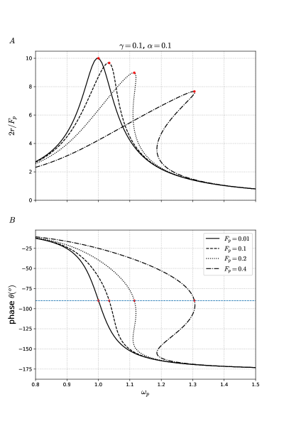
Figure 1: $\mathbf{A}$ Nonlinear resonant curves as obtained from Eq. (5) via numerical continuation (see Appendix A). The scaled response amplitude ($2r/F_{p}$) is represented as a function of the angular pump frequency $\omega_{p}$. For low pump amplitude, the peak of the resonant curve tends to the quality factor $Q=\gamma^{-1}=10$, consistent with the linear oscillator resonant curve. As the pump amplitude increases, the nonlinear effects become more relevant. The red dots are analytical approximations of the resonant peaks. $\mathbf{B}$ Duffing oscillator response phase dependence on the drive frequency $\omega_{p}$ as obtained from Eq. (6). The horizontal dashed line corresponds to the phase angle delay $-90^{\circ}$ of the oscillator response with respect to the driving force.

II.1 Analysis of the Duffing amplifier response to the signal

We now perform a linear response analysis of the oscillator to the presence of the external signal, when $F_{s}\neq 0$, in Eq. (4). We use the following notation $u(t)=\bar{u}+u_{1}(t)$ and $v(t)=\bar{v}+v_{1}(t)$, where $\bar{u}$ and $\bar{v}$ are fixed-point solutions of Eq. (4) with $F_{s}=0$. This results in

$$\dot{u_{1}} = \frac{-1}{2\omega_{p}}\left\{\gamma\omega_{p}u_{1}+\Omega v_{1}+3\alpha\left[2\bar{u}\bar{v}u_{1}+(\bar{u}^{2}+3\bar{v}^{2})v_{1}\right]/4-F_{s}\sin\phi(t)\right\},$$

$$\dot{v_{1}} = \frac{-1}{2\omega_{p}}\left\{-\Omega u_{1}+\gamma\omega_{p}v_{1}-3\alpha\left[(\bar{v}^{2}+3\bar{u}^{2})u_{1}+2\bar{u}\bar{v}v_{1}\right]/4+F_{s}\cos\phi(t)\right\}.$$ (8)

Using the harmonic balance method, in which we assume $u_{1}(t)=\tilde{u}_{1}e^{i\delta t}+\tilde{u}_{1}^{*}e^{-i\delta t}$ and $v_{1}(t)=\tilde{v}_{1}e^{i\delta t}+\tilde{v}_{1}^{*}e^{-i\delta t}$, we obtain

$$i\delta\tilde{u}_{1} = \frac{-1}{2\omega_{p}}\left\{\gamma\omega_{p}\tilde{u}_{1}+\Omega\tilde{v}_{1}+3\alpha\left[2\bar{u}\bar{v}\tilde{u}_{1}+(\bar{u}^{2}+3\bar{v}^{2})\tilde{v}_{1}\right]/4+iF_{s}e^{i\phi_{0}}/2\right\},$$

$$i\delta\tilde{v}_{1} = \frac{-1}{2\omega_{p}}\left\{-\Omega\tilde{u}_{1}+\gamma\omega_{p}\tilde{v}_{1}-3\alpha\left[(\bar{v}^{2}+3\bar{u}^{2})\tilde{u}_{1}+2\bar{u}\bar{v}\tilde{v}_{1}\right]/4+F_{s}e^{i\phi_{0}}/2\right\}.$$ (9)

This algebraic linear system may be recast as

$$\left(\begin{array}[]{c}\tilde{u}_{1}\\ \tilde{v}_{1}\end{array}\right)=-\frac{F_{s}e^{i\phi_{0}}}{4\omega_{p}(ad-bc)}\left(\begin{array}[]{cc}d&-b\\ -c&a\end{array}\right)\left(\begin{array}[]{c}i\\ 1\end{array}\right),$$ (10)

where the coefficients are

$$a = i\delta+\gamma/2+\frac{3\alpha\bar{u}\bar{v}}{4\omega_{p}},$$

$$b = \frac{\Omega+3\alpha(\bar{u}^{2}+3\bar{v}^{2})/4}{2\omega_{p}},$$

$$c = -\frac{\Omega+3\alpha(\bar{v}^{2}+3\bar{u}^{2})/4}{2\omega_{p}}$$

$$d = i\delta+\gamma/2-\frac{3\alpha\bar{u}\bar{v}}{4\omega_{p}}.$$

The response of the oscillator may be written approximately as

$$x(t)=\bar{u}\cos(\omega_{p}t)-\bar{v}\sin(\omega_{p}t)+u_{s}\cos[(\omega_{p}+\delta)t]-v_{s}\sin\left[(\omega_{p}+\delta)t\right]+u_{i}\cos[(\omega_{p}-\delta)t]-v_{i}\sin\left[(\omega_{p}-\delta)t\right],$$ (11)

where $u_{s}=\mbox{Re}[\tilde{u}_{1}]-\mbox{Im}[\tilde{v}_{1}]$, $v_{s}=\mbox{Im}[\tilde{u}_{1}]+\mbox{Re}[\tilde{v}_{1}]$, $u_{i}=\mbox{Re}[\tilde{u}_{1}]+\mbox{Im}[\tilde{v}_{1}]$, and $v_{i}=-\mbox{Im}[\tilde{u}_{1}]+\mbox{Re}[\tilde{v}_{1}]$. The terms at frequency $\omega_{p}$ correspond to the pump response, the terms at $\omega_{p}+\delta$ are known as the signal response, and the terms at $\omega_{p}-\delta$ are known as the idler response.

We can define the gains in decibels of the Duffing amplifier response with respect to the signal excitation in decibels as

$$G_{p} =20\log\frac{X_{p}}{F_{s}},$$ (12)

$$G_{s} =20\log\frac{X_{s}}{F_{s}},$$

$$G_{i} =20\log\frac{X_{i}}{F_{s}},$$

where $X_{p}=\sqrt{u^{2}+v^{2}}$, $X_{s}=\sqrt{u_{s}^{2}+v_{s}^{2}}$, and $X_{i}=\sqrt{u_{i}^{2}+v_{i}^{2}}$.

In Fig. 2, we show a time series of the numerical integration of the Duffing amplifier equations of motion given in Eq. (1). The envelope is obtained from the averaging method via Eq. (4). In Fig. 3, we compare the gains of pump, signal, and idler responses as defined in Eq. (12). Very good agreement between numerical results and the linear response predictions, as given in Eqs. (10)-(12), are obtained.

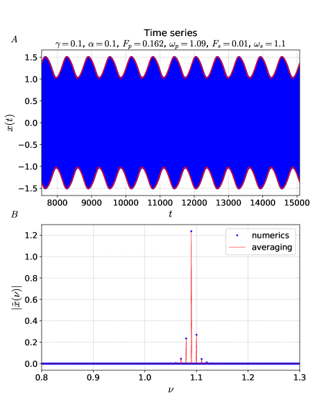
Figure 2: A Time series at the cusp point of the bistability region. The envelope is given by $\sqrt{u(t)^{2}+v(t)^{2}}$, which can be obtained from the linear response result of Eq. (4). B The corresponding Fourier transform. We again obtain good agreement between numerical results with averaging method predictions.

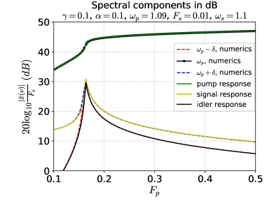
Figure 3: Spectral components as function of $F_{p}$. Numerical and analytical (linear response) results are plotted together. The analytical results are obtained from Eqs. (10)-(12). The peaks in the signal and idler gains occur near the saddle-node bifurcation which is at the cusp of the bistability region.

III The underdamped ac-driven Duffing oscillator with added white noise

III.1 Stochastic resonance

The time evolution of the forced Duffing oscillator in the presence of dissipation and noise is given by

$$\ddot{x}+x=-\gamma\dot{x}-\alpha x^{3}+F_{p}\cos(\omega_{p}t)+R(t),$$ (13)

where the Gaussian noise $R(t)$ obeys $\langle R(t)\rangle=0$ and $\langle R(t)R(t^{\prime})\rangle=2D\delta(t-t^{\prime})$. We then assume the response of the Duffing oscillator can be split in two parts: one coherent and the other stochastic, such as

$$x(t)=A_{p}e^{i\omega_{p}t}+A^{*}_{p}e^{-i\omega_{p}t}+\delta x(t),$$ (14)

where $\delta x(t)$ is the response to the input noise. We obtain approximately the following differential algebraic system

$$\delta\ddot{x} = -\delta x-\gamma\delta\dot{x}-\alpha\left(6|A_{p}|^{2}+\overline{\delta x^{2}}_{\infty}\right)\delta x+R(t),$$ (15)

$$A_{p} = \frac{F_{p}}{2\left[\Omega+i\gamma\omega_{p}+3\alpha\left(|A_{p}|^{2}+\overline{\delta x^{2}}_{\infty}\right)\right]},$$ (16)

where we neglected the superharmonics and made the approximation $\delta x^{3}\approx\overline{\delta x^{2}}_{\infty}\delta x$ for the random fluctuations in Eq. (15). The average $\overline{\delta x^{2}}_{\infty}$ is the equilibrium quadratic fluctuation of the stochastic process deviate $\delta x$ and is given by

$$\overline{\delta x^{2}}_{\infty}=\frac{D/\gamma}{1+\alpha\left(6|A_{p}|^{2}+\overline{\delta x^{2}}_{\infty}\right)}.$$

The stationary solution is given by

$$\overline{\delta x^{2}}_{\infty} =\frac{-(1+6\alpha|A_{p}|^{2})+\sqrt{(1+6\alpha|A_{p}|^{2})^{2}+4\alpha D/\gamma}}{2\alpha},$$ (17)

$$|A_{p}| =\frac{F_{p}}{2\sqrt{\left[\Omega+3\alpha\left(|A_{p}|^{2}+\overline{\delta x^{2}_{\infty}}\right)\right]^{2}+\gamma^{2}\omega_{p}^{2}}}.$$

One can observe in Eq. (17) that a back-action effect occurs between the fluctuations due to noise and the oscillator fundamental harmonic amplitude. As a consequence, there is a shift of the resonance peak of the oscillator pump response, i.e. $|A_{p}|$, to higher frequencies as can be seen in Fig. 4 when compared to resonant curves of Fig. 1A. This shift increases with increasing noise level. The red dots correspond closely to the resonant peaks in which $\Omega+3\alpha(|A_{p}|^{2}+\overline{\delta x^{2}_{\infty}})=0$. In Fig. 5, we see that the region of bistability decreases and is displaced to higher frequencies and higher pump amplitudes. This effect implies that stochastic resonance can only occur in our system when the driving pump frequency is blue-shifted in relation to the natural frequency of the oscillator, i.e. $\Omega<0$, as can be seen in Fig. 6. Simply speaking, SR occurs when the bistability region passes by or near a parameter-space point $(\omega_{p},F_{p})$ when the noise level $D$ is increased. This back-action effect is due to the cubic nonlinearity of the Duffing oscillator and to the fact that the squared deviate $\delta x^{2}(t)$ has a finite average. We also would like to point out that as the noise level is increased the bistability width in pump frequency decreases in qualitative agreement with the experimental work by Aldridge and Cleland Aldridge and Cleland (2005). This is expected since bistability is a coherent response of the nonlinear oscillator to the pump which decreases in amplitude and range when the noise level increases.

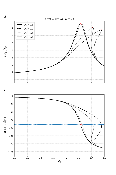
Figure 4: $\mathbf{A}$ Effect of noise on resonance curves. The curves are blue shifted and the peaks are reduced when noise is added with respect to the equivalent results, with $D=0$, in Fig. 1. Furthermore, some curves with bistability, when $D=0$, are reduced or devoid of bistability when $D=0.3$. The red dots are analytical approximations of the resonant peaks. $\mathbf{B}$ Duffing oscillator response phase dependence on the drive frequency $\omega_{p}$ as obtained from Eq. (16). The horizontal dashed line corresponds to the phase angle delay $-90^{\circ}$ of the oscillator response with respect to the driving force.

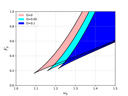
Figure 5: Comparison of bistability regions (shaded) of the Duffing oscillator without white noise, based on Eq. (5), and with white noise, based on Eqs. (17). The parameters are $\gamma=0.1$ and $\alpha=0.1$.

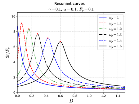
Figure 6: Resonance curves as a function of $D$. The curves are obtained from Eq. (17) of the Duffing oscillator response to a pump with angular frequency $\omega_{p}$. The red dots are analytical approximations of the resonance peaks.

III.2 Noise spectral density and signal-to-noise ratio

With the appropriate modifications, the power spectral density of the stationary stochastic process $\delta x(t)$, as governed by Eq. (15), can be written as

$$S_{\delta x}(\nu)=\int_{-\infty}^{\infty}\langle\delta x(t+\tau)\delta x(t)\rangle\,e^{-i\nu\tau}d\tau=\frac{2D}{\left(\nu^{2}-\nu_{0}^{2}\right)^{2}+\gamma^{2}\nu^{2}},$$ (18)

where $\nu_{0}^{2}=1+\alpha\left(6|A_{p}|^{2}+\overline{\delta x^{2}_{\infty}}\right)$, $A_{p}$ and $\overline{\delta x^{2}_{\infty}}$ are determined in Eq. (17). The signal-to-noise ratio (SNR) is given by

$$SNR_{p}=\frac{4|A_{p}|^{2}}{S_{\delta x}(\omega_{p})}$$ (19)

In Fig. 7, we show the noise spectral density for various values of pump frequencies. We note that the peaks here are detuned compared to the corresponding resonance peaks of the pump response amplitude $|A_{p}|$ from Fig. 6. There are no units for $S_{\delta x}$ or $D$ because we nondimensionalized our equations. In Fig. 8, we can see stochastic resonance in the SNR as a function of the noise level $D$. We notice that it only occurs when the oscillator is driven by a blue-shifted pump. Furthermore, the effect grows with increasing detuning up to roughly $\omega_{p}=2.35$ (not shown here). After that the peaks in SNR start reducing. In addition, for such high detuning, the noise level $D$ necessary for the appearance of SR is considerably higher.

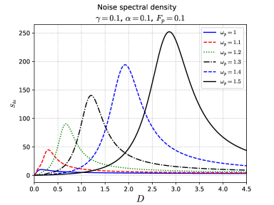
Figure 7: Noise spectral density curves obtained from Eq. (18) for various values of pump frequency as a function of noise level $D$.

Figure 8: SNR curves obtained from Eq. (19) for various values of pump frequency as a function of noise level $D$. The peaks in these curves are characteristic of stochastic resonance.

IV The Duffing amplifier with added white noise

We now proceed to evaluate estimates of signal-to-noise ratio (SNR) of the system described by the following dynamics

$$\ddot{x}+x=-\gamma\dot{x}-\alpha x^{3}+F_{p}\cos(\omega_{p}t)+F_{s}\cos(\omega_{s}t+\phi)+R(t).$$ (20)

We start our analysis of this stochastic differential equation seeking a stationary solution of the type

$$x(t)=x_{p}(t)+x_{s}(t)+x_{i}(t)+\delta x(t),$$ (21)

in which the coherent responses are

$$x_{p}(t) =A_{p}e^{i\omega_{p}t}+A_{p}^{*}e^{-i\omega_{p}t},$$

$$x_{s}(t) =A_{s}e^{i\omega_{s}t}+A_{s}^{*}e^{-i\omega_{s}t},$$

$$x_{i}(t) =A_{i}e^{i\omega_{i}t}+A_{i}^{*}e^{-i\omega_{i}t}.$$

After removing the coherent evolution part from Eq. (20), we obtain the following Langevin equation for the stochastic variable $\delta x(t)$

$$\delta\ddot{x}+\delta x+\gamma\delta\dot{x}+\alpha\left[6\xi_{0}^{2}+\overline{\delta x^{2}}_{\infty}\right]\delta x=R(t),$$ (22)

where

$$\xi_{0}^{2}=|A_{p}|^{2}+|A_{s}|^{2}+|A_{i}|^{2}.$$ (23)

The average of the stationary stochastic variable $\delta x(t)$ squared is given by

$$\overline{\delta x^{2}}_{\infty}=\frac{D/\gamma}{1+\alpha\left(6\xi_{0}^{2}+\overline{\delta x^{2}}_{\infty}\right)},$$

whose solution in terms of $\xi_{0}^{2}$ is

$$\overline{\delta x^{2}}_{\infty}=\frac{-(1+6\alpha\xi_{0}^{2})+\sqrt{(1+6\alpha\xi_{0}^{2})^{2}+4\alpha D/\gamma}}{2\alpha}.$$ (24)

Using the harmonic balance method in Eq. (20), we obtain the algebraic system

$$G_{p}A_{p} =F_{p}/2-6\alpha A_{i}A_{s}A_{p}^{*}=F_{p}/2+18\alpha^{2}|A_{s}|^{2}|A_{p}|^{2}A_{p}/G_{i},$$ (25)

$$G_{s}A_{s} =-3\alpha A_{i}^{*}A_{p}^{2}+F_{s}e^{i\phi}/2=9\alpha^{2}|A_{p}|^{4}A_{s}/G_{i}^{*}+F_{s}e^{i\phi}/2,$$

$$G_{i}A_{i} =-3\alpha A_{s}^{*}A_{p}^{2}.$$

We also used the following shorthand notation

$$G_{p}(\omega_{p},|A_{p}|^{2},|A_{s}|^{2},|A_{i}|^{2}) =\Omega_{p}+3\alpha\left(|A_{p}|^{2}+2|A_{s}|^{2}+2|A_{i}|^{2}+\overline{\delta x^{2}_{\infty}}\right)+i\gamma\omega_{p},$$ (26)

$$G_{s}(\omega_{s},|A_{p}|^{2},|A_{s}|^{2},|A_{i}|^{2}) =\Omega_{s}+3\alpha\left(2|A_{p}|^{2}+|A_{s}|^{2}+2|A_{i}|^{2}+\overline{\delta x^{2}_{\infty}}\right)+i\gamma\omega_{s},$$

$$G_{i}(\omega_{i},|A_{p}|^{2},|A_{s}|^{2},|A_{i}|^{2}) =\Omega_{i}+3\alpha\left(2|A_{p}|^{2}+2|A_{s}|^{2}+|A_{i}|^{2}+\overline{\delta x^{2}_{\infty}}\right)+i\gamma\omega_{i},$$

in which the detunings are given by $\Omega_{p}=1-\omega_{p}^{2}$, $\Omega_{i}=1-\omega_{i}^{2}$, and $\Omega_{s}=1-\omega_{s}^{2}$.

We can simplify the algebraic system given in Eqs. (25) and obtain the equations for $|A_{p}|^{2}$, $|A_{s}|^{2}$, and $|A_{i}|^{2}$, which are given by

$$|A_{p}|^{2} =\frac{F_{p}^{2}}{4\left|G_{p}-18\alpha^{2}|A_{s}|^{2}|A_{p}|^{2}/G_{i}\right|^{2}},$$ (27)

$$|A_{s}|^{2} =\frac{F_{s}^{2}}{4\left|G_{s}-9\alpha^{2}|A_{p}|^{4}/G_{i}^{*}\right|^{2}},$$

$$|A_{i}|^{2} =9\alpha^{2}|A_{s}|^{2}|A_{p}|^{4}/|G_{i}|^{2}.$$

In Fig. 9, we plot the main spectral components of the Duffing amplifier as a function of $F_{p}$ in the presence of noise. These results are obtained from numerically solving the system of equations (24) and (27) using the method of Gauss-Newton Nocedal and Wright (2006). Notice that the peaks in the signal and idler gains are reduced compared to the case in which there is no noise, $D=0$, as portrayed in Fig. 3. This occurs because due to the presence of noise the bistability region moves further away in parameter space, as can be seen in Fig. 5, hence the amplification decreases.

In Fig. 10, we plot the main spectral components of the Duffing amplifier scaled by $F_{p}$ as a function of the noise level $D$. These results are obtained from numerically solving the system of equations (24) and (27).

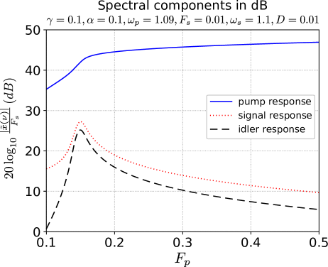
Figure 9: Main spectral components of the Duffing amplifier as a function of $F_{p}$ in the presence of noise. These results are obtained from numerically solving Eqs. (27) for each value of the noise level $D$. The peaks in the signal and idler gains occur near the cusp point of the bistability region. As the noise level increases, the bistability region becomes further away in parameter space, as can be seen in Fig. 5, hence the amplification decreases as compared with the results presented in Fig. 3.

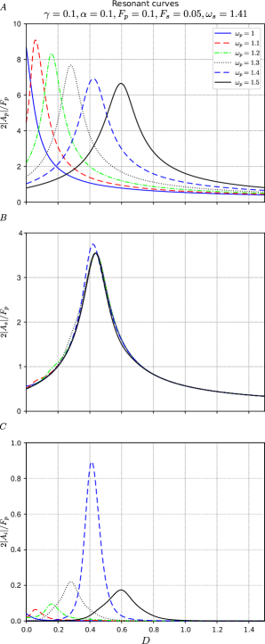
Figure 10: Duffing amplifier coherent response resonance curves as a function of the noise level $D$. The curves are obtained from Eq. (27) for the Duffing amplifier response to the simultaneous pump and signal coherent excitations and also to the added white noise. In frame $\mathbf{A}$, we show the pump responses to several values of pump frequency. In frame $\mathbf{B}$, we show the signal responses and in frame $\mathbf{C}$, the idler responses. In all responses we see clearly the occurrence of stochastic resonance.

IV.1 Noise spectral density and signal-to-noise ratios

With the appropriate modifications, the power spectral density of the stationary stochastic process $\delta x(t)$, as governed by Eq. (22), can be written as

$$S_{\delta x}(\nu)=\int_{-\infty}^{\infty}\langle\delta x(t+\tau)\delta x(t)\rangle\,e^{-i\nu\tau}d\tau=\frac{2D}{\left[\nu^{2}-1-\alpha\left(6\xi_{0}^{2}+\overline{\delta x^{2}_{\infty}}\right)\right]^{2}+\gamma^{2}\nu^{2}},$$ (28)

where $\xi^{2}$ is determined in Eq. (23) and $\overline{\delta x^{2}_{\infty}}$ by Eq. (24). We can obtain then three measures of signal-to-ratio (SNR), each one related to pump, signal, and idler responses. They are

$$SNR_{p} =\frac{4|A_{p}|^{2}}{S_{\delta x}(\omega_{p})},$$ (29)

$$SNR_{s} =\frac{4|A_{s}|^{2}}{S_{\delta x}(\omega_{s})},$$

$$SNR_{i} =\frac{4|A_{i}|^{2}}{S_{\delta x}(\omega_{i})}.$$

In Fig. 11, we show the noise spectral density (NSD) for various values of pump frequencies for pump, signal, and idler frequencies. There is considerable dispersion in the peaks of pump and idler NSDs, but not in the signal NSD. We note that the peaks here are detuned compared to the corresponding resonance peaks of the pump response amplitude $|A_{p}|$ from Fig. 10. There are no units for $S_{\delta x}$ or $D$ because we nondimensionalized our equations. In Fig. 12, we can see stochastic resonance in the SNR at pump ($\mathbf{A}$), signal ($\mathbf{B}$), and idler ($\mathbf{C}$) frequencies as a function of the noise level $D$.

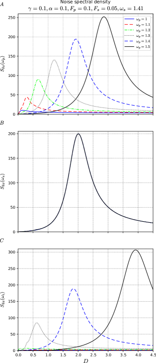
Figure 11: Noise spectral density curves at pump, signal, and idler frequencies obtained from Eq. (28) for various values of pump frequency as a function of noise level $D$.

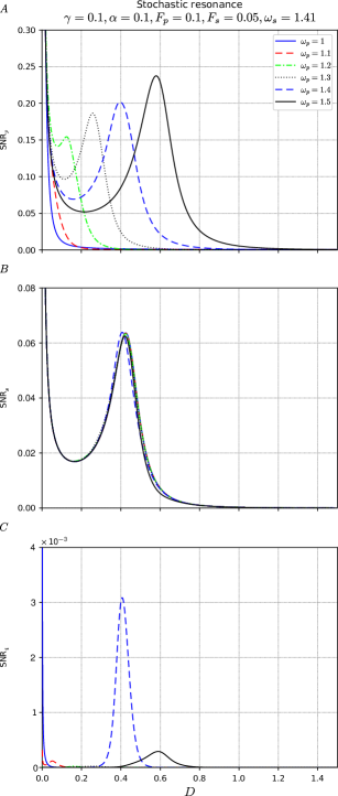
Figure 12: SNR curves obtained from Eq. (29) for various values of pump frequency as a function of noise level $D$.

V Conclusion

Here, we briefly reviewed the theory on the dynamics of the ac-driven Duffing oscillator with damping and the Duffing amplifier. Afterwards, we investigated the effect of added white noise on the driven Duffing oscillator and on the Duffing amplifier. We proposed a simple approximate theoretical model to account for the effects of coherent drive and added noise on the nonlinear system that goes beyond the linear response theory. We assumed that the response of the nonlinear system to these inputs can be split into coherent and stochastic parts that influence on one another. We predict a blue shift in frequency (when the Duffing constant is positive) and also a shift towards higher pump values of the bistability region that are due to increased noise levels. For a constant value of pump amplitude, the range of bistability tends to decrease with increasing noise levels. This was observed experimentally by Aldridge and Cleland Aldridge and Cleland (2005) and is in qualitative agreement with our results. A more quantitative agreement could be found if one uses the Euler-Bernoulli beam theory and the parameters of their resonator to obtain the coefficients of the Duffing oscillator. An outline of this method can be seen in the Appendix B. In addition to these results, with our proposed model, we showed that the coherent response and the noise spectral density have resonance peaks at very different noise levels. Due to this, there is a peak in SNR indicating that SR occurs. We point out that the observed SR is related to the shifting of the bistability region as the noise level is increased. We have seen that in our system a necessary condition for SR to occur is that the pump frequency has to be blue-shifted with respect to the natural frequency of the nonlinear resonator. Furthermore, we notice that our model predicted SR in underdamped monostable driven Duffing oscillators, but we emphasize that it could also be used to investigate SR in under- or over-damped bistable Duffing oscillators.

We also predicted with semi-analytical methods that SR occurs in the pump, signal, and idler responses of the Duffing amplifier. For each of these cases, we calculated the coherent response amplitude squared and the NSD. Again, as the coherent amplitude peaks occur at very different values of noise levels than the NSD’s peaks, a peak in the SNR appears and this is characteristic of SR. We also saw that the pump, signal, and idler SR peaks usually occur at different values of noise levels.

We believe that the theoretical framework we developed here to obtain the response to noise in the driven Duffing oscillator and in the Duffing amplifier can be adapted to other nonlinear oscillators and amplifiers. Quantitative predictions should be possible, once one obtains physical parameters from micro or nanomechanical resonators. For example, one could investigate how the noise spectral density that was measured in a parametrically-driven resonator by Miller et al. Miller et al. (2020) will change when nonlinearities are present. Another issue in parametric amplifiers is the presence of nonlinear dissipation Papariello et al. (2016); Li and Shaw (2020). How these systems behave when white noise is added to them seems to be an open problem.

Particularly relevant systems to be investigated for the effect of added noise are nonlinear resonators that can present frequency-comb spectra Ganesan et al. (2017, 2018); Batista and Lisboa de Souza (2020). We believe that the method we developed here may help evaluate the robustness of mechanical frequency-comb generation in the presence of noise.

Appendix A Numerical continuation

We solve numerically Eq. (5) for a range of pump frequency values using the method of numerical continuation. We call

$$h(x,\omega_{p})=x\left[\left(\Omega+3\alpha x\right)^{2}+\gamma^{2}\omega_{p}^{2}\right]-F_{p}^{2}/4,$$

We notice that the dynamics

$$\dot{x} =-\frac{\partial h}{\partial\omega_{p}},$$ (30)

$$\dot{\omega}_{p} =\frac{\partial h}{\partial x},$$

keeps $h(x(t),\omega_{p}(t))$ constant. This is a Hamiltonian dynamics where $h$ is the Hamiltonian. In the present case, the partial derivatives are given by

$$\frac{\partial h}{\partial x} =(\gamma\omega_{p})^{2}+(\Omega+3\alpha x)^{2}+6\alpha x(\Omega+3\alpha x),$$

$$\frac{\partial h}{\partial\omega_{p}} =x\omega_{p}\left[-2(\Omega+3\alpha x)+\gamma^{2}\right].$$

At $t=0$, we choose $h(x(0),\omega_{p}(0))=0$. To avoid numerical difficulties, we normalize the flow in Eq. (30), such that the speed $\sqrt{\dot{x}^{2}+\dot{\omega}_{p}^{2}}=1$.

Appendix B Single-degree-of-freedom theory

Here, we show how to obtain a single-degree-of-freedom (SDOF) model from a physical system such as a mechanical resonator, which could be a cantilever or a doubly-clamped beam. The simplest theory to describe the flexural vibrations of a thin beam is the Euler–Bernoulli beam theory Landau et al. (1986). In this theory the bending motion is described by the equation

$$\mu\frac{\partial^{2}X}{\partial t^{2}}=-EI\frac{\partial^{4}X}{\partial z^{4}},$$ (31)

where $X(z,t)$ represents the lateral deflections from equilibrium at a point $z$ along the length of the beam at a time $t$. In this equation, $\mu$ is the linear density of the beam (with units of mass over length), $E$ is the Young’s modulus, and $I$ is the area moment of inertia and in a prismatic rod it is given by

$$I=\frac{{\mathcal{W}}\tau^{3}}{12},$$ (32)

where ${\mathcal{W}}$ is the width and $\tau$ is the thickness. Using the method of separation of variables, we can write down the $n$-th normal-mode solution of Eq. (31) as $X(z,t)=X_{n}(z)\cos(\omega_{n}t+\varphi)$, where $n=0,1,2,\dots$. Hence, we obtain the differential equation for the amplitude $X_{n}(z)$, which is

$$\frac{d^{4}X_{n}}{dz^{4}}=\frac{\mu\omega_{n}^{2}}{EI}X_{n}.$$ (33)

The most general solution to this equation is

$$X_{n}(z)=A_{n}\cos(k_{n}z)+B_{n}\sin(k_{n}z)+C_{n}\cosh(k_{n}z)+D_{n}\sinh(k_{n}z),$$ (34)

in which $k_{n}=\left(\frac{\mu\omega_{n}^{2}}{EI}\right)^{1/4}$. The coefficients of this solution are determined by the boundary conditions. Please see table 1 for the main types of boundary conditions used in nanomechanics.

Type of resonator	Boundary conditions	Characteristic equation	Fundamental-mode eigenvalue
Clamped-clamped	$X_{n}(0)=X_{n}^{{}^{\prime}}(0)=0$ $X_{n}(\ell_{0})=X_{n}^{{}^{\prime}}(\ell_{0})=0$	$\cos(k_{n}\ell_{0})\cosh(k_{n}\ell_{0})=1$	$4.730041$
Clamped-free	$X_{n}(0)=X_{n}^{{}^{\prime}}(0)=0$ $X_{n}^{{}^{\prime\prime}}(\ell_{0})=X_{n}^{{}^{\prime\prime\prime}}(\ell_{0})=0$	$\cos(k_{n}\ell_{0})\cosh(k_{n}\ell_{0})=-1$	1.875104

Table 1: Thin prismatic beam resonator boundary conditions with corresponding characteristic equation and fundamental-mode eigenvalue of flexural vibrations.

From the $n$-th root $x_{n}$ of the characteristic equations in table 1, we obtain the normal mode frequencies of oscillation from the following expression

$$f_{n} =\frac{1}{2\pi}\sqrt{\frac{EI}{\mu}}k_{n}^{2}=\frac{x_{n}^{2}\tau}{2\pi\ell_{0}^{2}}\sqrt{\frac{E}{12\rho}}.$$ (35)

The potential elastic energy of the bent bar Landau et al. (1986) can be written as

$$U_{el}=\frac{EI}{2}\int\kappa(s)^{2}ds,$$

where $s$ is the arclength parameterization and $\kappa(s)$ is the curvature. In terms of $X(z)$, it can be written as

$$\kappa(s)=\frac{X^{\prime\prime}(z)}{(1+X^{\prime}(z)^{2})^{3/2}},$$

while $ds=\sqrt{1+X^{\prime}(z)^{2}}dz$. Hence, we can write the potential energy approximately as a single-degree-of-freedom (SDOF) polynomial as

$$\frac{\kappa(z)X^{2}(z,t)}{2}+\frac{A(z)X^{4}(z,t)}{4}\simeq\frac{EI}{2}\int_{0}^{\ell_{0}}\frac{X^{\prime\prime 2}}{\left(1+X^{\prime 2}\right)^{5/2}}dz^{\prime}$$ (36)

$$\approx\frac{EI}{2}\int_{0}^{\ell_{0}}X^{\prime\prime 2}\left[1-\frac{5}{2}X^{\prime 2}\right]dz^{\prime},$$

where the exact energy functional was approximated by a Taylor expansion of the denominator. We now use the first normal mode approximation $X(z,t)=X_{0}(z)\cos(\omega t)$ to find analytical expressions for the coefficients. Based on the orthogonality condition of the Fourier expansion terms $\cos(n\omega t)$, we are able to determine the coefficients above. Hence, we find the coefficients of the SDOF potential energy polynomial to be given by

$$\kappa(z) =\frac{EI}{X_{0}(z)^{2}}\int_{0}^{\ell_{0}}X_{0}^{\prime\prime}(z^{\prime})^{2}dz^{\prime}=\frac{EIx_{0}^{4}}{X_{0}(z)^{2}\ell_{0}^{4}}\int_{0}^{\ell_{0}}X_{0}(z^{\prime})^{2}dz^{\prime},$$ (37a)

$$A(z) =-\frac{5EI}{X_{0}(z)^{4}}\int_{0}^{\ell_{0}}\left[X_{0}^{\prime\prime}(z^{\prime})X_{0}^{\prime}(z^{\prime})\right]^{2}dz^{\prime}$$ (37b)

Using the first normal-mode solution, Eq. (34), we find that the effective mass for the fundamental normal mode at height $z$ Batista et al. (2018) is

$$m_{0}^{eff}(z)=\frac{\mu}{X_{0}(z)^{2}}\int_{0}^{\ell_{0}}X_{0}(z^{\prime})^{2}dz^{\prime}.$$ (38)

The Newton’s equation of motion for the SDOF approximation is given by

$$m_{eff}\frac{d^{2}X}{ds^{2}}+\kappa X=-\Gamma\frac{dX}{ds}-AX^{3}+{\mathcal{F}}_{p}\cos(\bar{\omega}_{p}s)+{\mathcal{F}}_{s}\cos(\bar{\omega}_{s}s+\phi)+R(s).$$ (39)

In dimensionless units, we find Eq. (20), where the parameters are

$$\omega_{0}^{2} =\frac{\kappa}{m_{eff}},$$ (40)

$$t =\omega_{0}s,$$

$$x(t) =\frac{X(t)}{L},$$

$$\omega_{p} =\frac{\bar{\omega}_{p}}{\omega_{0}},$$

$$\omega_{s} =\frac{\bar{\omega}_{s}}{\omega_{0}},$$

$$\gamma =\frac{\Gamma}{m_{eff}\omega_{0}},$$

$$\alpha =\frac{AL^{2}}{m_{eff}\omega_{0}^{2}},$$

$$F_{p} =\frac{{\mathcal{F}}_{p}}{m_{eff}\omega_{0}^{2}},$$

$$F_{s} =\frac{{\mathcal{F}}_{s}}{m_{eff}\omega_{0}^{2}},$$

$$r(t) =\frac{R(s)}{m_{eff}\omega_{0}^{2}},$$

where $L$ is a characteristic length of the problem. It should be chosen in such a way that the coefficient $\alpha$ is small, otherwise the perturbative methods used in this paper may not work.

References

- Benzi et al. (1981) R. Benzi, A. Sutera, and A. Vulpiani, Journal of Physics A: mathematical and general 14, L453 (1981).
- Longtin (1993) A. Longtin, Journal of Statistical Physics 70, 309 (1993).
- Ikemoto et al. (2018) S. Ikemoto, F. DallaLibera, and K. Hosoda, Neurocomputing 277, 29 (2018).
- McNamara et al. (1988) B. McNamara, K. Wiesenfeld, and R. Roy, Physical Review Letters 60, 2626 (1988).
- Hibbs et al. (1995) A. Hibbs, A. Singsaas, E. Jacobs, A. Bulsara, J. Bekkedahl, and F. Moss, Journal of Applied Physics 77, 2582 (1995).
- Mantegna and Spagnolo (1994) R. N. Mantegna and B. Spagnolo, Physical Review E 49, R1792 (1994).
- Badzey and Mohanty (2005) R. L. Badzey and P. Mohanty, Nature 437, 995 (2005).
- Jeffries and Wiesenfeld (1985) C. Jeffries and K. Wiesenfeld, Phys. Rev. A 31, 1077 (1985).
- Wiesenfeld (1985) K. Wiesenfeld, J. of Stat. Phys. 38, 1071 (1985).
- Wiesenfeld and McNamara (1985) K. Wiesenfeld and B. McNamara, Phys. Rev. Lett. 55, 13 (1985).
- Wiesenfeld and McNamara (1986) K. Wiesenfeld and B. McNamara, Phys. Rev. A 33, 629 (1986).
- Aldridge and Cleland (2005) J. S. Aldridge and A. N. Cleland, Phys. Rev. Lett. 94, 156403 (2005).
- R. Almog, S. Zaitsev, O. Shtempluck, and Buks (2007) R. Almog, S. Zaitsev, O. Shtempluck, and E. Buks, Appl. Phys. Lett. 90, 013508 (2007).
- Ochs et al. (2021) J. S. Ochs, M. Seitner, M. I. Dykman, and E. M. Weig, Physical Review A 103, 013506 (2021).
- McNamara and Wiesenfeld (1989) B. McNamara and K. Wiesenfeld, Physical review A 39, 4854 (1989).
- Dykman et al. (1995) M. I. Dykman, D. G. Luchinsky, R. Mannella, P. V. E. McClintock, N. D. Stein, and N. G. Stocks, Il Nuovo Cimento D 17, 661 (1995).
- Gammaitoni et al. (1998) L. Gammaitoni, P. Hänggi, P. Jung, and F. Marchesoni, Rev. Mod. Phys. 70, 223 (1998).
- Alfonsi et al. (2000) L. Alfonsi, L. Gammaitoni, S. Santucci, and A. R. Bulsara, Physical Review E 62, 299 (2000).
- Kang et al. (2003) Y.-M. Kang, J.-X. Xu, and Y. Xie, Physical Review E 68, 036123 (2003).
- Landa et al. (2008) P. S. Landa, I. A. Khovanov, and P. V. E. McClintock, Physical Review E 77, 011111 (2008).
- Stocks et al. (1993) N. G. Stocks, N. D. Stein, and P. V. E. McClintock, Journal of Physics A: Mathematical and General 26, L385 (1993).
- Landau and Lifshitz (1980) L. D. Landau and E. M. Lifshitz, Statistical Physics, 3rd ed. (Pergamon Press, 1980).
- Dykman et al. (1990) M. I. Dykman, R. Mannella, P. V. E. McClintock, S. M. Soskin, and N. G. Stocks, Physical Review A 42, 7041 (1990).
- Czaplewski et al. (2018) D. A. Czaplewski, C. Chen, D. Lopez, O. Shoshani, A. M. Eriksson, S. Strachan, and S. W. Shaw, Phys. Rev. Lett. 121, 244302 (2018).
- Ganesan et al. (2017) A. Ganesan, C. Do, and A. Seshia, Phys. Rev. Lett. 118, 033903 (2017).
- Ganesan et al. (2018) A. Ganesan, C. Do, and A. Seshia, Applied Physics Letters 112, 021906 (2018).
- Singh et al. (2020) R. Singh, A. Sarkar, C. Guria, R. J. Nicholl, S. Chakraborty, K. I. Bolotin, and S. Ghosh, Nano Letters 20, 4659–4666 (2020).
- Batista and Lisboa de Souza (2020) A. A. Batista and A. A. Lisboa de Souza, Journal of Applied Physics 128, 244901 (2020).
- R. Almog, S. Zaitsev, O. Shtempluck, and Buks (2006) R. Almog, S. Zaitsev, O. Shtempluck, and E. Buks, Appl. Phys. Lett. 88, 213509 (2006).
- Batista et al. (2008) A. A. Batista, F. A. Oliveira, and H. N. Nazareno, Phys. Rev. E 77, 066216 (2008).
- Nocedal and Wright (2006) J. Nocedal and S. Wright, Numerical optimization (Springer Science & Business Media, 2006).
- Miller et al. (2020) J. M. Miller, D. D. Shin, H.-K. Kwon, S. W. Shaw, and T. W. Kenny, Applied Physics Letters 117, 033504 (2020).
- Papariello et al. (2016) L. Papariello, O. Zilberberg, A. Eichler, and R. Chitra, Physical Review E 94, 022201 (2016).
- Li and Shaw (2020) D. Li and S. W. Shaw, Nonlinear Dynamics 102, 2433 (2020).
- Landau et al. (1986) L. D. Landau, E. M. Lifshitz, L. P. Pitaevskii, and A. M. Kosevich, Theory of Elasticity (Pergamon Press, 1986).
- Batista et al. (2018) A. A. Batista, C. E. R. da Silva, and A. A. Lisboa de Souza, Eur. J. Phys. 39, 055009 (2018).