June 9, 2021

^∗ Corresponding authors.
^∗ Hue Sun Chan. E-mail: chan@arrhenius.med.utoronto.ca
^∗ Jianhui Song. E-mail: jhsong@qust.edu.cn

——————————————————————————————————————–

TOC Graphics

Abstract

An accurate account of disordered protein conformations is of central importance to deciphering the physico-chemical basis of biological functions of intrinsically disordered proteins and the folding-unfolding energetics of globular proteins. Physically, disordered ensembles of non-homopolymeric polypeptides are expected to be heterogeneous; i.e., they should differ from those homogeneous ensembles of homopolymers that harbor an essentially unique relationship between average values of end-to-end distance $R_{\rm EE}$ and radius of gyration $R_{\rm g}$. It was posited recently, however, that small-angle X-ray scattering (SAXS) data on conformational dimensions of disordered proteins can be rationalized almost exclusively by homopolymer ensembles. Assessing this perspective, chain-model simulations are used to evaluate the discriminatory power of SAXS-determined molecular form factors (MFFs) with regard to homogeneous versus heterogeneous ensembles. The general approach adopted here is not bound by any assumption about ensemble encodability, in that the postulated heterogeneous ensembles we evaluated are not restricted to those entailed by simple interaction schemes. Our analysis of MFFs for certain heterogeneous ensembles with more narrowly distributed $R_{\rm EE}$ and $R_{\rm g}$ indicates that while they deviates from MFFs of homogeneous ensembles, the differences can be rather small. Remarkably, some heterogeneous ensembles with asphericity and $R_{\rm EE}$ drastically different from those of homogeneous ensembles can nonetheless exhibit practically identical MFFs, demonstrating that SAXS MFFs do not afford unique characterizations of basic properties of conformational ensembles in general. In other words, the ensemble to MFF mapping is practically many-to-one and likely non-smooth. Heteropolymeric variations of the $R_{\rm EE}$–$R_{\rm g}$ relationship were further showcased using an analytical perturbation theory developed here for flexible heteropolymers. Ramifications of our findings for interpretation of experimental data are discussed.

INTRODUCTION

A detailed characterization of the conformational properties of disordered protein states is essential for many areas of biophysical and biomedical research. These include, but are not limited to, the thermodynamic balance between folded and unfolded states of globular proteinsTrewhella1992 ; julie1995 ; Plaxco1999 ; shortle2001 ; shimizu2002 ; tobin2004 ; plaxco2004 ; rose2004 ; haran2006 ; eaton2007 ; MarshJulie2009 ; DanRohit2013 ; raleighBJ2018 and the relationships between myriad biological functions of the increasing repertoire of intrinsically disordered proteins (IDPs) and the behaviors of their conformational ensembles.borg07 ; tanja08 ; schuler10 ; tanja2010 ; fuzzy12 ; marsh12 ; baoxu2014 ; martin2016 ; zhirong2016a ; zhirong2016b ; AlexRohitRev2018 One basic property of disordered conformational ensembles is their extent in space. This property, often referred to as conformational dimensions, is of central importance to protein science because it bears on the very nature of the folding/unfolding cooperativity of globular proteinschanetal2004 ; fersht2009 ; chanetal2011 ; munoz2012 ; TaoPCCP ; Reddy2016 ; DT_TiBS2-19 as well as, for example, the spatial ranges and other configurational features of biomolecular interactions involving IDPsPGW2000 ; zhirong2009 ; Veronika2017 including those of highly disordered “fuzzy” dynamic IDP complexes.sigalov_etal2007 ; kragelund2008 ; tanja2014 ; sigalov2016 ; wu_etal2017 ; Amin_etal2020 Recent advances in the studies of biomolecular condensatescliff2017 ; rosen2017 ; lin_biochemrev suggest further that conformational dimensions of individual IDP molecules may serve as an indicator of the propensity of the IDP to undergo liquid-liquid phase separation.Amin_etal2020 ; lin2017 ; jeetainPNAS ; joanJPCL ; rohitBJ2020 Indeed, despite the low-spatial-resolution information they provide directly, measures of conformational dimensions of disordered protein states such as end-to-end distance and radius of gyration (denoted, respectively, as $R_{\rm EE}$ and $R_{\rm g}$ hereafter) offer fundamental insights into the microscopic physical interactions underlying protein behaviorsDavidShaw2 ; cosb15 and thus provide critical assessments of the extent to which current molecular dynamics force fields are adequate for capturing the physics of these interactions.sarah15 ; sarah17 ; best2017 ; shea2017 ; DEShaw2018 ; joan2021

Small-angle X-ray scattering (SAXS) is a commonly utilized technique in biophysicsdoniachRev2001 ; SAXS-Complex ; AndoChemRev2017 to quantify conformational dimensions of disordered proteins by measuring $R_{\rm g}$ and related ensemble-averaged spatial properties.Trewhella1992 ; Plaxco1999 ; tobin2004 ; plaxco2004 ; tobinkevinJMB2012 ; OsmanJMB2014 ; SvergunFEBSLett ; tobinkevinPNAS2015 ; antonov2016 ; benPNAS2016 ; tanja2021 Because SAXS takes into account simultaneously many positions along the entire chain molecule, SAXS affords information complementary to techniques such as Förster resonance energy transfer (FRET)haran2006 ; eaton2007 ; schuler10 ; baoxu2014 ; haran2012 ; schulerCOSB2013 ; blanchard2014 ; rhoades2014 ; deniz2014 ; arash2015 ; rhoades2016 ; rhoades2016 ; schulerAnnuRev2016 that probe only one or a few relative positions at a time. Nonetheless, since scattering intensities are averaged over different chain conformations in an ensemble, SAXS data do not provide detailed spatial information of individual conformations. Therefore, models and assumptions often need to be invoked to relate SAXS data to putative conformational ensembles that likely—though not necessarily—underlie the experimental data. Recently, the generality of some of these assumptions, or lack thereof, has been brought into a sharper focus. One of the reasons is that for several disordered protein states, the $R_{\rm g}$s extracted from SAXS using Guinier analysis disagree significantly with the $R_{\rm g}$ values inferred from single-molecule FRET (smFRET) data by assuming that the underlying conformational distribution is Gaussian.tobinkevinJMB2012 ; tobinkevinPNAS2015 ; dt2009 ; SchulerJCP2013 ; Songetal2015

As weSongetal2015 ; Songetal2017 and otherslemke2017 ; raleighPNAS2019 have noted, besides improving the treatment of excluded volume in the underlying baseline homopolymer chain modeldomb1965 ; fisher1966 ; cloizeaux1974 ; oono_ren81-3 used in SAXS and smFRET data analysisSchulerBestJCP2018 ; zhengbest2018 [see, e.g., Eq. (5.6) of ref. (83)], the apparent mismatches between SAXS- and smFRET-inferred $R_{\rm g}$s should be fundamentally reconcilable by recognizing that conformational ensembles of proteins are heterogeneousSongetal2017 ; Vendruscolo2007 ; Lyle_etal_2013 ; RuffHolehouse ; best2020 in that they do not necessarily resemble those of homopolymers, because proteins are heteropolymeric sequences of different amino acid residues. Simply put, proteins are not homopolymers. Therefore, the relationship between their average $R_{\rm EE}$ and their average $R_{\rm g}$ can differ from that of homopolymers, i.e., the relation can be different from that posited by Gaussian chain and other homopolymeric models.Songetal2015 ; Songetal2017 It is possible, then, for heterogeneous conformational ensembles to embody both a smFRET-inferred average $R_{\rm EE}$ and a SAXS-determined average $R_{\rm g}$ that are not coupled in the same way as for homopolymers.Songetal2015 ; Songetal2017 ; lemke2017 This conceptual framework has been applied to rationalize experimental data with apparent success.Songetal2015 ; lemke2017 ; raleighPNAS2019 ; claudiu2016 ; claudiu2017 ; GregJACS2020

In this context, it is notable that recent experimental developments emphasize that one should be able to glean more structural information about disordered protein ensembles from SAXS data than merely extracting the mean square radius of gyration, $\langle R^{2}_{\rm g}\rangle$, by using Guinier analysis, which relies on scattering intensity, $I(q)$, at small $q$ values, with $q=|{\bf q}|$ being the magnitude of the scattering vector ${\bf q}$. In contrast, some of the recent SAXS studies of disordered protein ensembles consider Kratky plots, or molecular form factors (MFFs), over a substantially wider range of $q$ (refs. (93; 94; 95; 96)). Logically, the more enriched information provided by MFFs, namely the $I(q)$ at larger $q$s, is expected to impose more experimental constraints on putative, theoretically constructed conformational ensembles beyond merely requiring them to have a given $\langle R^{2}_{\rm g}\rangle$. Accordingly, this recognition raises basic questions as to whether theoretical/computational heterogeneous conformational ensembles constructed to satisfy a given $\langle R^{2}_{\rm g}\rangle$ and a given $\langle R^{2}_{\rm EE}\rangle$ remain viable when MFFs are taken into account; that is, whether those putative heterogeneous ensembles are also consistent with the additional information afforded by the larger-$q$ behaviors of experimental MFFs. To address this and related questions, it should be recognized first that although MFFs provide more structural information on disordered protein ensembles than Guinier analysis, MFFs still involve extensive averaging over individual conformations and therefore an MFF by itself is far from being able to uniquely define a disordered conformational ensemble. With these considerations in mind, we seek here to clarify the information content of SAXS-determined MFFs by investigating the compatibility of various putative conformational ensembles with given MFFs. As will be apparent below, this delineation is useful toward establishing a more rigorous perimeter for interpreting SAXS-determined MFFs of disordered proteins in terms of heterogeneous conformational ensembles.

To this end, we use explicit-chain simulations of a coarse-grained polypeptide modelSongetal2015 to construct extensive sets of different heterogeneous ensembles with properties selected systematically for the insights they would provide. We then compare their MFFs with those of full ensembles of homopolymers embodying varying degrees of uniform intrachain attractive or repulsive interactions, paying special attention to identify and evaluate scenarios in which the MFFs of heterogeneous and homogeneous ensembles are highly similar. Building on prior advances, we commence this effort with a survey of the $(R_{\rm g},R_{\rm EE})$ subensembles introduced previously to address the apparent SAXS–smFRET mismatches in $R_{\rm g}$ measurement.Songetal2015 ; Songetal2017 ; DICE Each of these subensembles is individually a heterogenoues conformational ensemble because it is defined to be a small part of a homogeneous ensemble and therefore not a homogeneous ensemble by itself. Interestingly, while the MFFs of different subensembles sharing the same $R_{\rm g}$ with the $\langle R^{2}_{\rm g}\rangle^{1/2}$ of the homogeneous ensemble differ among themselves because the MFF depends on the subensemble’s $R_{\rm EE}$, the MFFs of some subensembles are quite similar to the MFF of the full homogeneous ensemble.

Besides the $(R_{\rm g},R_{\rm EE})$ subensembles, other heterogeneous ensembles with more diverse conformations, i.e., not limited to a very narrow range of $R_{\rm g},R_{\rm EE}$ values, are also assessed. Motivated partly by experimental evidence suggesting that disordered protein ensembles are heterogeneous in a sequence-sensitive mannerDanRohit2013 ; GregJACS2020 (sometimes manifested by peculiar forms of the inferred $R_{\rm g}$ distributiontanja2010 ) despite their homopolymer-like overall average $R_{\rm g}$ values,raleighPNAS2019 ; raleighBiochem2020 we study several physically plausible, conformationally diverse heterogeneous ensembles with narrower distributions of $R_{\rm g}$ than that of a homogeneous ensemble. Quite surprisingly, these heterogeneous ensembles nonetheless lead to MFFs very similar to that of the corresponding homogeneous ensemble. Indeed, we even come across other mathematically intriguing cases where heterogeneous ensembles drastically different from homopolymers yet possess MFFs that are essentially identical to MFFs of homopolymers. These comparisons indicate that the MFFs of homogeneous ensembles and some heterogeneous ensembles can be practically indistinguishable when experimental uncertainties are allowed for, underscoring the desirability of employing additional experiment techniques complementary to SAXS to better characterize disordered protein ensembles.lemke2017 ; raleighPNAS2019 ; GregJACS2020 Aiming for rudimentary insights into the complex sequence-ensemble relationship of heteropolymeric disordered proteins, we have also developed an extension of theoretical perturbative approachesfixman1955 ; fixman1962a ; fixman1962b ; Edwards1965 ; tanaka1966 ; ohta81 ; Freedbook ; ohta82 ; muthu84 ; chanJCP89 ; chanJCP90 to calculate $\langle R^{2}_{\rm g}\rangle^{1/2}$, $\langle R^{2}_{\rm EE}\rangle^{1/2}$, scattering intensity $I(q)$, and MFF$(q\langle R^{2}_{\rm g}\rangle^{1/2})$ for heteropolymers. Predictions of this analytical formulation allow for a preliminary understanding of how sequence-specific interactions may encode heterogeneous ensembles that share the same $\langle R^{2}_{\rm g}\rangle^{1/2}$ but differ in other aspects of their conformational distributions such as their root-mean-square end-to-end distance $\langle R^{2}_{\rm EE}\rangle^{1/2}$. Details of these findings are provided below.

MODELS AND METHODS

The present coarse-grained C_α protein model (one bead per monomer, or per residue) and the sampling algorithm are based on the formulation used in our previous investigations of smFRET interpretation for disordered proteins.Songetal2015 ; Songetal2017 As before, a polypeptide chain is modeled as a chain of $n$ beads labeled by $i=1,2,\dots,n$ at position ${\bf R}_{i}$, with C_α–C_α virtual bond length $b=|{\bf r}_{i,i+1}|\equiv|{\bf R}_{i+1}-{\bf R}_{i}|=3.8$ Å between connected beads. The bond-angle potential energy $U_{\rm bond}(\{{\bf r}\})=\sum_{i=2}^{n-1}\epsilon_{\theta}(\theta_{i}-\theta_{0})^{2}$, where $\epsilon_{\theta}=10.0k_{\rm B}T$, $\theta_{i}=\cos^{-1}({\bf r}_{i,i-1}\cdot{\bf r}_{i,i+1}/b^{2})$ is the virtual bond angle at bead $i$, $\theta_{0}=106.3^{\circ}$ is the reference bond angle corresponding to the most populated virtual bond angle in the Protein Data Bank,levitt1976 $k_{\rm B}$ is Boltzmann constant, and $T$ is absolute temperature. The potential energy for excluded volume is given by $U_{\rm SAW}(\{{\bf r}\})=(1/2)\sum_{i=1}^{n}\sum_{j=1}^{n}(U_{\rm SAW})_{ij}(r_{ij})$ where “SAW” stands for self-avoiding walk and $(U_{\rm SAW})_{ij}\equiv\epsilon_{\rm ex}(R_{\rm hc}/r_{ij})^{12}$. In this expression, $r_{ij}\equiv|{\bf R}_{j}-{\bf R}_{i}|$ is the distance between beads $i$ and $j$, and $\epsilon_{\rm ex}=1.0k_{\rm B}T$ is the self-avoiding excluded-volume repulsion strength used in our model. As in many simulation studies of protein foldingchanetal2011 and in most of the cases we considered in refs. (76) and (77), a hard-core repulsion distance $R_{\rm hc}=4.0$ Å is adopted. In addition to the non-bonded excluded-volume repulsive term, here we consider also homopolymeric, uniform intrachain non-bonded attractive or repulsive interactions given by $U_{\rm p}(\epsilon_{\rm p},r_{0};\{{\bf r}\})=\sum_{i=1}^{n}\sum_{j=i+3}^{n}(U_{\rm p})_{ij}(\epsilon_{\rm p},r_{0};r_{ij})$ where $(U_{\rm p})_{ij}(\epsilon_{\rm p},r_{0};r_{ij})\equiv\epsilon_{\rm p}\;\exp[-(r_{ij}/r_{0})^{2}]$ to account for polypeptides under different solvent conditions. For computational efficiency, all non-bonded potential energy terms are set to zero for $r_{ij}\geq 10.0$ Å. Illustrative examples of a combination of excluded-volume and $\epsilon_{\rm p}$-dependent attractive or repulsive interactions are provided in Fig. 1. In the analysis below, we refer to the $\epsilon_{\rm p}=0$ case as the SAW model, and the case with $\epsilon_{\rm p}=0$ as well as with $U_{\rm SAW}$ turned off (effectively setting $\epsilon_{\rm ex}=0$) as the Gaussian chain model. Theoretical predictions reported in this work are for chain length $n=75$, which we have usedSongetal2017 to address experimental SAXS and smFRET data on Protein L (refs. (59; 62)). By using this chain length, new findings are amenable to comparison with previous results. In the present context, however, $n=75$ is taken merely as an exemplifying case for proteins of similar lengths because the focus of this study is on general principles rather than any particular protein.

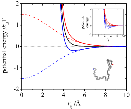
Figure 1: Non-bonded interactions in the coarse-grained chain model. The total pairwise potential energy (solid red or blue curves) between two monomers $i,j$ that are not directly connected along the polymer chain ($|i-j|>1$) is the sum of the repulsive SAW potential $(U_{\rm SAW})_{ij}$ (solid black curves) and a pairwise attractive ($\epsilon_{\rm p}<0$, blue) or repulsive ($\epsilon_{\rm p}>0$, red) interaction $(U_{\rm p})_{ij}(\epsilon_{\rm p},r_{0};r_{ij})$ ($r_{0}=3.8$ Å, dashed curves). This interaction reduces to the SAW potential when $\epsilon_{\rm p}=0$ (see text for details). $(U_{\rm p})_{ij}(\epsilon_{\rm p},r_{0};r_{ij})$ is given here for $\epsilon_{\rm p}/k_{\rm B}T=\pm 1.5$ as an example. The total non-bonded potentials for $\epsilon_{\rm p}/k_{\rm B}T=\pm 0.5$, $\pm 1.0$, $\pm 2.0$, and $\pm 2.5$ are provided by the inset as further illustrations. An example conformation is shown for the $n=75$ model polymer utilized in the present investigation. The red and blue beads mark the chain termini, positions corresponding to those of FRET dyes for determining $R_{\rm EE}$ in our previous study.Songetal2017

Chain conformations are sampled at $T=300$ K using standard Metropolis Monte Carlo techniquesMC described before,song13 wherein equal a priori probabilities are assigned to pivot and kink jumps,stockmayer1962 ; Lal69 with acceptance rate of $\approx 30\%$ for the attempted chain moves.Songetal2015 ; Songetal2017 For each simulation, the first $10^{7}$ attempted moves for equilibration are not used for the calculation of average conformational properties. Subsequently, $\sim 10^{9}$ moves are attempted to sample $\sim 10^{7}$ conformations (snapshots taken every 100 attempted moves) for further analysis. Among other ensemble properties to be described in the Results section below, radius of gyration $R_{\rm g}=[n^{-1}\sum_{i=1}^{n}|{\bf R}_{i}-{\bf R}_{\rm cm}|^{2}]^{1/2}$ (where ${\bf R}_{\rm cm}$ is the center of mass or centroid position, ${\bf R}_{\rm cm}=n^{-1}\sum_{i=1}^{n}{\bf R}_{i}$) and end-to-end distance $R_{\rm EE}=|{\bf R}_{n}-{\bf R}_{1}|$ are computed from the sampled conformations. Examples of the distribution of $R_{\rm g},R_{\rm EE}$ populations for several different values of the intrachain interaction energy parameter $\epsilon_{\rm p}$ are shown in Fig. 2. As expected, when intrachain interaction is attractive ($\epsilon_{\rm p}<0$), the distribution shifts to smaller $R_{\rm g}$ and $R_{\rm EE}$ (Fig. 2b,c) relative to the SAW distribution ($\epsilon_{\rm p}=0$, Fig. 2a), whereas the distribution shifts to larger $R_{\rm g}$ and $R_{\rm EE}$ when intrachain interaction is repulsive ($\epsilon_{\rm p}>0$, Fig. 2d).

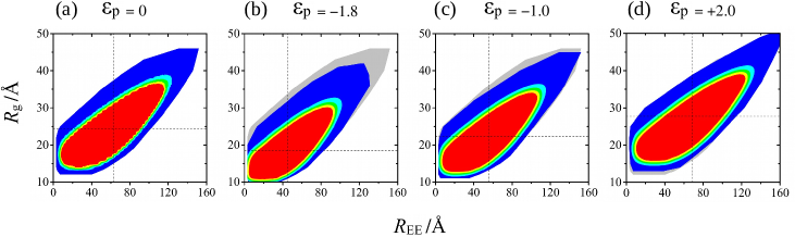
Figure 2: Radius of gyration and end-to-end distance distributions of $\epsilon_{\rm p}$-dependent homopolymers of various compactness. Joint distributions of $R_{\rm g}$ and $R_{\rm EE}$ (color coded) are shown for $n=75$ conformational ensembles at representative $\epsilon_{\rm p}$ values as indicated ($\epsilon_{\rm p}$ given in units of $k_{\rm B}T$ hereafter). The profile of the SAW [$\epsilon_{\rm p}=0$, (a)] distribution is included as a gray background in the other three $\epsilon_{\rm p}\neq 0$ distributions [(b)–(d)] for comparison. For each ensemble, the root-mean-square $\langle R_{\rm g}^{2}\rangle^{1/2}$ and $\langle R_{\rm EE}^{2}\rangle^{1/2}$ are marked by the horizontal and vertical dotted lines respectively. A total of $10^{7}$ conformations are sampled for each distribution. Numbers of conformations are recorded for all $R_{\rm g}$–$R_{\rm EE}$ bins of $1{\rm\AA}\times 1{\rm\AA}$ and are color-coded as follows. White: 0, blue: [1–200), cyan: [200–400), green: [400–600), yellow: [600–800), and red: $\geq 800$ conformations.

Fig. 3 provides an overview of the properties of the $\epsilon_{\rm p}$-dependent homogeneous conformational ensembles that are used as baselines in work. Fig. 3a shows that for these homogeneous ensemble, $\langle R^{2}_{\rm g}\rangle/\langle R^{2}_{\rm EE}\rangle$ is essentially constant at $\approx 0.16$ for SAW ($\epsilon_{\rm p}=0$) and ensembles with repulsive interactions ($\epsilon_{\rm p}>0$), and the ratio increases as the ensembles become more compact with attractive interactions ($\epsilon_{\rm p}$ more negative), reaching $\approx 0.36$ for $\epsilon_{\rm p}=-5.0$. This trend is in line with the simulated $\langle R_{\rm g}\rangle/\langle R_{\rm EE}\rangle$ values of $\approx 0.41$ for SAWs of comparable lengths and a rough estimate of $\langle R_{\rm g}\rangle/\langle R_{\rm EE}\rangle$ of $0.71$ for conformations in the shape of a compact sphereSongetal2015 because $0.41^{2}=0.17$ and $0.71^{2}=0.50$ although $\langle R^{2}_{\rm g}\rangle/\langle R^{2}_{\rm EE}\rangle\neq(\langle R_{\rm g}\rangle/\langle R_{\rm EE}\rangle)^{2}$ ($\langle\dots\rangle$ represents averaging over a given ensemble). The scaling of intrachain distance $r_{ij}$ of these ensembles in the form of $\langle r^{2}_{ij}\rangle^{1/2}\sim|i-j|^{\nu}$ is shown in Fig. 3b and the estimated $\epsilon_{\rm p}$-dependent $\nu$ exponents are provided in Fig. 3c. The tendency for the scaling exponents for smaller $|i-j|$ (red diamonds in Fig. 3c) to be slightly higher than those for larger $|i-j|$ (black circles in Fig. 3c) is in line with that seen in recent simulation results (e.g., Fig. 3A of ref. (93)) and is consistent with excluded-volume effects leading to a lower contact probability when the contacting monomers are in the middle of the chain than when the contact is between the two ends of the chain (with different loop-closure exponents).chanJCP89 ; chanJCP90 ; cloizeaux1980 Because $\langle R^{2}_{\rm g}\rangle^{1/2}$ is determined by $\epsilon_{\rm p}$ for these homopolymer ensembles, the essentially one-to-one mapping between $\epsilon_{\rm p}$ and $\nu$ in Fig. 3c (aside from the small differences for small and large $|i-j|$s) is translated into an essentially one-to-one mapping between $\langle R^{2}_{\rm g}\rangle^{1/2}$ and $\nu$ in Fig. 3d. Disordered protein ensembles inferred from experiments have sometimes been characterized by homopolymer scaling exponent $\nu$ as a proxy for measured $\langle R^{2}_{\rm g}\rangle^{1/2}$ in recent studies.SchulerBestJCP2018 ; zhengbest2018 ; tobinSci2017 ; tobinPNAS2019 ; zheng_etal_JPCL2020 It should be recognized, however, that for real proteins which are heteropolymers, there is no universal correspondence between $\langle R^{2}_{\rm g}\rangle^{1/2}$ and $\nu$, as exemplified by recent studies of the N-terminal domain of the ribosomal protein L9 (NTL9)raleighPNAS2019 and the C-terminal domain of the same protein.raleighBiochem2020 In principle, when a conformational ensemble is sufficiently heterogeneous, $\nu$ may not be well-defined even when the chain dimensions are similar to those of SAWs (see below).

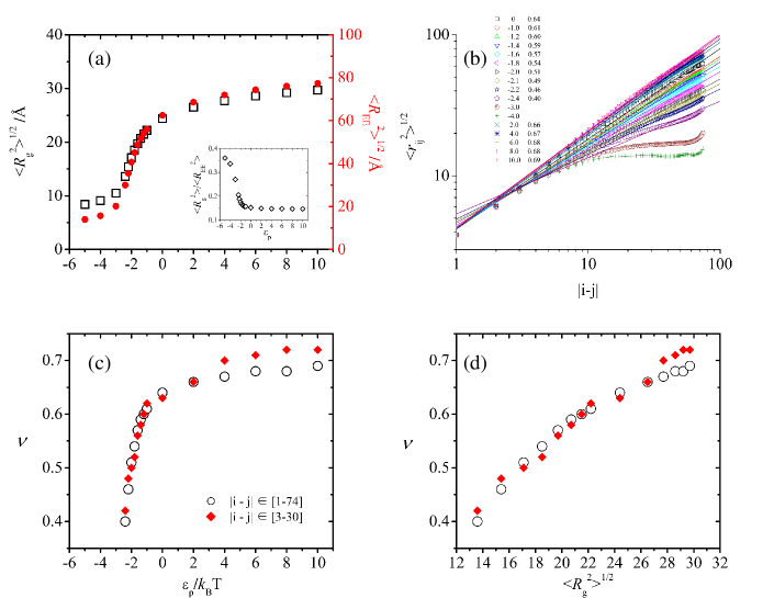
Figure 3: Compactness-dependent homopolymer properties. Dimensional features of conformational ensembles with $U_{\rm SAW}+U_{\rm p}$ interactions are obtained as functions of $\epsilon_{\rm p}$. (a) Root-mean-square radius of gyration, $\langle R^{2}_{\rm g}\rangle^{1/2}$ (black squares, left vertical scale), and end-to-end distance, $\langle R^{2}_{\rm EE}\rangle^{1/2}$ (red circles, right vertical scale). The $\epsilon_{\rm p}$-dependent ratio of mean-square $R_{\rm g}$ to mean-square $R_{\rm EE}$ is provided in the inset. (b) Variation of root-mean-square intrachain monomer-monomer distance $\langle r^{2}_{ij}\rangle^{1/2}$ with sequence separation $|i-j|$. Averages are based on $10^{5}$ sampled conformations for each $\epsilon_{\rm p}$. The legend provides the symbols (left column) for different $\epsilon_{\rm p}$ values (middle column) together with the scaling exponents, $\nu$ (right column), obtained by fitting $\langle r^{2}_{ij}\rangle^{1/2}\sim|i-j|^{\nu}$ to the plotted data for each $\epsilon_{\rm p}$. No $\nu$ values are fitted to the $\langle r^{2}_{ij}\rangle^{1/2}$ vs $|i-j|$ data for $\epsilon_{\rm p}=-3.0$ and $-4.0$ because of their significant deviations from linearity. (c) Scaling exponents $\nu$ from (b) by fitting $\langle r^{2}_{ij}\rangle^{1/2}$ data for all sequence separations ($1\leq|i-j|\leq 74$, black circles) and by fitting only part of the data for smaller sequence separations ($3\leq|i-j|\leq 30$, red diamonds). (d) Variation of scaling exponents in (c) with root-mean-square $R_{\rm g}$.

The scattering intensity $I(q)$ of the homogeneous and heterogeneous conformational ensembles considered in this study is computed using the Debye formulaAndoChemRev2017

$$I(q)=4\pi\int_{0}^{\infty}dr\;P(r)\frac{\sin(qr)}{qr}\;,$$ (1)

where $q=|{\bf q}|$ is the magnitude of the scattering vector ${\bf q}$,

$$P(r)=\frac{1}{n^{2}}\sum_{i=1}^{n}\sum_{j=1}^{n}\langle\delta(r-r_{ij})\rangle$$ (2)

is the pair distance distribution function obtained by averaging over bead-bead distances $r_{ij}$ of sampled conformations, $\delta$ denotes the Dirac delta function, and $1/n^{2}$ is the normalization factor for the total number of $i,j$ pairs. Because our focus is on general physical principles, we consider beads in our coarse-grained chain model as simple point-like scattering centers, neglecting complexities arising from atomic form factors and solvation in computational studies that utilize more atomistic representations of the polypeptide chain.AndoChemRev2017 ; SaliFoXS Inasmuch as a sufficient large number of conformations are used, our simulated $I(q)$s are numerically robust, as we have verified by comparing $I(q)$s computed using $1,000$, $10,000$, or $100,000$ sampled conformations in selected cases. Practically, the upper limit of $\infty$ for the integration in Eq. 1 may be replaced by the longest pairwise distance, $r_{\rm max}$, in the system, which is approximately equal to $(n-1)b\sin(\theta_{0}/2)\approx 225.0$Å when an $n=75$ chain in our model adopts an all-trans conformation.

The simulated scattering intensities $I(q)$ of the homopolymer ensembles in Fig. 3 normalized by $I(0)\equiv I(q=0)=4\pi$ are shown in Fig. 4a, the $I(q)/I(0)$ for Gaussian chains is also included for comparison. These curves are similar to those obtained for other models for disordered proteins.tobinSci2017 Their corresponding dimensionless Kratky plots (MFFs) are provided in Fig. 4b. Here the vertical variable $I(q)/I(0)$ is scaled by $q^{2}\langle R^{2}_{\rm g}\rangle$ and the horizontal variable $q$ is scaled by $\langle R^{2}_{\rm g}\rangle^{1/2}$, where $\langle R^{2}_{\rm g}\rangle$ is the mean square radius of gyration determined by the sampled conformations used for the calculation of $I(q)$ for the same ensemble. By definition, all dimensionless Kratky plots are essentially identical in the small-$q$ Guinier regime irrespective of $\langle R^{2}_{\rm g}\rangle^{1/2}$, as can be seen for the examples in Fig. 4b, because $I(q)/I(0)\rightarrow\exp(-q^{2}\langle R^{2}_{\rm g}\rangle/3)$ for $q\rightarrow 0$ (ref. (58)) and therefore the dimensionless vertical variable always behaves approximately as $x^{2}\exp(-x^{2}/3)$ for small $x$ where $x=q\langle R^{2}_{\rm g}\rangle^{1/2}$ is the dimensionless horizontal variable.

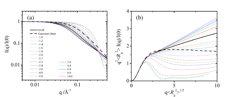
Figure 4: Compactness-dependent scattering properties of homopolymer ensembles. (a) Log-log plot of scattering intensity $I(q)$ (normalized by value at $q=0$) as a function of the magnitude of the scattering vector, $q$, and (b) dimensionless Kratky plots (MFFs) are shown for $n=75$ SAW (solid black curve), Gaussian-chain (dashed black curve), and homopolymer ensembles defined by various $\epsilon_{\rm p}\neq 0$. Results for the latter ensembles are depicted as color dashed curves for $\epsilon_{\rm p}<0$ and color solid curves for $\epsilon_{\rm p}>0$ as indicated by the legend in (a).

We note that all the $I(q)/I(0)$ curves for models with excluded volume in Fig. 4a (all except the Gaussian-chain black dashed curve), irrespective of their different $\epsilon_{\rm p}$ values, converge in a narrow region around $q\approx 0.3$Å^-1 (though the $I(q)/I(0)$ values do not converge at exactly the same $q$). This behavior of the model may be understood by recognizing that these models, even for very different $\epsilon_{\rm p}$, should share essentially identical probabilities for two shortest distances dictated by the local bond structure that are independent of or minimally affected by the global $\epsilon_{\rm p}$-dependent conformational compactness. These distances are the virtual bond length between two sequential beads ($r_{i,i+1}=b=3.8$Å) and the distance between two beads separated by a single bead along the chain sequence ($r_{i-1,i+1}\approx 2b\sin(\theta_{0}/2)=6.08$Å). The virtual bond length is a constant in the model, whereas small variations in $r_{i-1,i+1}$ are possible because the virtual bond angle $\theta_{i}$ fluctuates around $\theta_{0}$ in accordance with a harmonic potential. The essential identical probabilities of these short distances among the models translate into a near-coincidence of their $I(q)/I(0)$ values around $q\approx\pi/2r_{i,i+1}=0.41$Å^-1 and $q\approx\pi/2r_{i,i+2}\approx 0.26$Å^-1 in reciprocal space, averaging to $q\approx 0.34$Å^-1 which is consistent with the approximate convergence observed in Fig. 4a. An approximate convergence of theoretical $I(q)/I(0)$ curves has also been seen in other studies, e.g., in Fig. 3B of ref. (93). In the latter case, the convergence is at $\approx 0.2$Å^-1, indicating that there are similarly probable distances $\approx\pi/(2\times 0.2$Å^-1)$=7.9$Å between scattering centers among the chain models in ref. (93) for different conformational compactness.

Examples of the homopolymer pair distance distribution functions $P(r)$ underlying the $I(q)$ functions in Fig. 4 are shown in Fig. 5. A notable shared feature among the different $P(r)$ plots in Fig. 5 as well as subsequent $P(r)$ plots in this article is the local $P(r)$ peaks at small $r$ values corresponding to the $r_{i,i+1}=b=3.8$Å and the $r_{i-1,i+1}\approx 2b\sin(\theta_{0}/2)=6.08$Å distances discussed above. As expected, aside from these common local peaks at small $r$s, the overall peak of the $P(r)$ distribution is shifted to smaller $r$ for increasingly negative $\epsilon_{\rm p}$ with a concomitant narrowing of the distribution. However, the shift to larger $r$ relative to the distribution for our SAW model is quite small for $\epsilon_{\rm p}>0$ because short-spatial-range contact-like repulsive potentials like those in our $\epsilon_{\rm p}>0$ models are essentially enhanced excluded volume interactions which, unsurprisingly, do not expand chain dimensions much beyond those of a SAW that already possesses a sizable excluded volume repulsion.

Figure 5: $\epsilon_{\rm p}$-dependent (with excluded volume) and Gaussian-chain distributions of intrachain monomer-monomer distances for $n=75$ homopolymers. As in Fig. 4, solid and dashed black curves are for, respectively, the SAW ($\epsilon_{\rm p}=0$, $\epsilon_{\rm ex}=1.0k_{\rm B}T$) and Gaussian-chain ($\epsilon_{\rm p}=\epsilon_{\rm ex}=0$) conformational ensembles. The correspondence between color curve styles and $\epsilon_{\rm p}\neq 0$ ensembles is identical to that in Fig. 4 as well; but, for clarity, $P(r)$ is plotted only for $\epsilon_{\rm p}=-2.4$, $-2.0$, $-1.8$, $-1.0$, and $+2.0$ in the present figure.

RESULTS

MFFs of heteropolymeric and homopolymeric SAWs are sometimes clearly distinct; but MFFs of select heterogeneous ensembles with very narrow ranges of ${\bm{R}}_{\bf g}$ and/or ${\bm{R_{\rm EE}}}$ can be very similar to MFFs of homopolymeric SAWs. We begin our analysis with three different hypothetical subensembles put forth previously as possible heterogeneous model conformational ensembles for Protein L with very narrow ranges of $R_{\rm EE}$ valuesSongetal2017 consistent with the experimental FRET efficiencies of $E\approx 0.75$ at [GuHCl] $=$ 1 M and $E\approx 0.45$ at [GuHCl] $=$ 7 M (Fig. 6). Two of the MFFs in Fig. 6 are for two subensembles sharing the same narrow range of $R_{\rm g}\approx 23.5$Å ($\langle R^{2}_{\rm g}\rangle^{1/2}$ $\approx$ $R_{\rm g}$ because of the narrow range) but with significantly different $R_{\rm EE}$s, namely $R_{\rm EE}\approx 46.5$Å for [GuHCl] $=$ 1 M (solid magenta curve) and $R_{\rm EE}\approx 56.9$Å for [GuHCl] $=$ 7 M (solid blue curve). These subensembles are of interest as examples of $R_{\rm g}$–$R_{\rm EE}$ decoupling,Songetal2017 ; lemke2017 in that the ensembles have the same $R_{\rm g}$ despite having very different $R_{\rm EE}$. Fig. 6 shows that their MFFs are distinct but similar in some notable respects. The MFF for the subensemble with smaller $R_{\rm EE}$ (magenta) is more oscillatory than that for the subensemble with larger $R_{\rm EE}$ (blue) for $2\lesssim q\langle R^{2}_{\rm g}\rangle^{1/2}\lesssim 7$ while the two MFFs converge at larger $q\langle R^{2}_{\rm g}\rangle^{1/2}$ values. Moreover, the MFFs of both of these subensembles—which are heterogeneous ensembles by construction—are quite similar to the MFF of a homopolymer ensemble with the same $\langle R^{2}_{\rm g}\rangle^{1/2}$ and an $\langle R^{2}_{\rm EE}\rangle^{1/2}$ corresponding approximately to the [GuHCl] $=$ 7 M case (black dashed curve). The differences among the MFFs are small except for $2\lesssim q\langle R^{2}_{\rm g}\rangle^{1/2}\lesssim 4$ which one may refer to as the “shoulder region” of the dimensionless Kratky curves. These comparisons indicate that, for some heterogeneous ensembles, different heterogenous and homogeneous ensembles entail different MFFs. In principle, therefore, these ensembles are distinguishable by SAXS measurements alone even though the ensembles share the same average $R_{\rm g}$. However, as seen in Fig. 6, the differences among some of the theoretical MFFs can be subtle. Thus, detectability of such differences may still be limited practically by uncertainties in experimental measurements. In contrast, the MFF for a subensemble with a smaller $\langle R^{2}_{\rm g}\rangle^{1/2}\approx 21.6$Å (dashed red curve) is clearly distinguishable from the other three MFFs because of its substantially lower $q^{2}\langle R^{2}_{\rm g}\rangle I(q)/I(0)$ for $q\langle R^{2}_{\rm g}\rangle^{1/2}\gtrsim 2$.

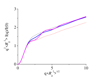
Figure 6: Theoretical MFFs pertinent to the case of Protein L at [GuHCl] = 1 and 7 M analyzed previously.Songetal2017 Dimensionless Kratky plots for $n=75$ heterogeneous conformational ensembles with (i) a sharp, $\delta$-function-like distribution with a narrow range of $R_{\rm g}$ centered at $23.5$ Å and a similarly sharp distribution of $R_{\rm EE}$ at $46.5$ Å (consistent with FRET efficiency $E=0.745$ when Förster radius $R_{0}=55$ Å, solid magenta curve), (ii) a sharp distribution of $R_{\rm EE}$ at $46.5$ Å (corresponding to $E=0.745$) but no restriction on $R_{\rm g}$ otherwise ($\langle R_{\rm g}^{2}\rangle^{1/2}=21.6$ Å, dashed red curve), and (iii) a sharp distribution of $R_{\rm EE}$ at $56.9$ Å (consistent with $E=0.447$) but no restriction on $R_{\rm g}$ otherwise ($\langle R_{\rm g}^{2}\rangle^{1/2}=23.4$ Å, solid blue curve) are compared with that for an $\epsilon_{\rm p}=-0.5$ homogeneous conformational ensemble with $\langle R_{\rm g}^{2}\rangle^{1/2}=23.5$ Å and $\langle R_{\rm EE}^{2}\rangle^{1/2}\approx 59.9$ Å (dashed black curve).

Fig. 7 provides a systematic comparison of SAXS signatures of SAW homopolymers with a broad distribution of $R_{\rm g}$ and $R_{\rm EE}$ on one hand against SAW subensembles each with a narrow range of $R_{\rm g}$ and/or a narrow range of $R_{\rm EE}$ on the other. Here we focus on subensembles with an $\langle R^{2}_{\rm g}\rangle^{1/2}\approx 24.5$Å (Fig. 7a) equals to the $\langle R^{2}_{\rm g}\rangle^{1/2}$ of the full homopolymeric SAW ensemble. As emphasized above, these subensembles are, by construction, heterogeneous conformational ensembles. It is noteworthy that despite the differences among the subensembles themselves and their drastically different $R_{\rm g}$–$R_{\rm EE}$ distributions vis-à-vis that of the full homopolymer ensemble (Fig. 7a), their $I(q)/I(0)$ versus $q$ plots appear to be quite similar aside from seemingly minor differences around $q\sim 0.1$Å^-1 (Fig. 7b). When presented as dimensionless Kratky plots (Fig. 7d), the differences in the shoulder region of the plots ($2\lesssim q\langle R^{2}_{\rm g}\rangle^{1/2}\lesssim 4$) for the different heterogeneous subensembles are more discernible. The subensembles’ different $I(q)$s are a reflection of their different pair distance distribution functions (Fig. 7c, Eq. 1). Among the subensembles with the same narrow range of $R_{\rm g}$ but different narrow ranges of $R_{\rm EE}$ in Fig. 7c, the peaks of the $P(r)$ of small-$R_{\rm EE}$ subensembles (dashed color curves) shift to larger $r$ values relative to the peak of the $P(r)$ for the homopolymer ensemble (solid black curve). Interestingly, the $P(r)$ of the subensemble with the largest $R_{\rm EE}\approx 88.5$Å among the subensembles considered is almost identical to the $P(r)$ of the homopolymer ensemble. Accordingly, their dimensionless Kratky plots essentially overlap (Fig. 7d, solid black and dashed dark-purple curves). In other words, quite remarkably, the SAXS signatures of these two very different disordered conformational ensembles—a highly heterogeneous ensemble with a narrow range of $R_{\rm g}$ as well as a narrow range of $R_{\rm EE}$ on one hand, and a homogeneous ensemble with a broad distribution of both $R_{\rm g}$ and $R_{\rm EE}$ on the other—are practically indistinguishable. Because $R_{\rm EE}\approx 88.5$Å is substantially larger than the $\langle R^{2}_{\rm EE}\rangle^{1/2}\approx 62.5$Å for the full homopolymer ensemble, it appears that inasmuch as effects on $P(r)$ are concerned, narrowing the broad distribution of $R_{\rm g}$ of the full homopolymer ensemble to a sharply peaked distribution around its $\langle R^{2}_{\rm g}\rangle^{1/2}$ value can be compensated by replacing the broad distribution of $R_{\rm EE}$ of the full homopolymer ensemble with a sharply peaked distribution around an $R_{\rm EE}$ value that is significantly larger than the $\langle R^{2}_{\rm EE}\rangle^{1/2}$ of the homopolymer ensemble.

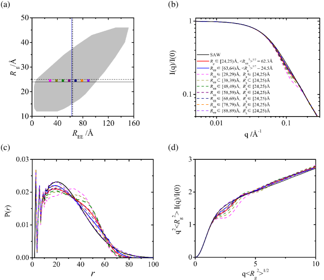
Figure 7: SAXS properties of subensembles of SAW chains. (a) The complete SAW homopolymer ensemble is represented by the gray area corresponding to the overall profile for $\epsilon_{\rm p}=0$ in Fig. 2; its $\langle R_{\rm EE}^{2}\rangle^{1/2}$ is indicated by the vertical blue solid line. The subensemble with a narrow $R_{\rm g}$ range, $24\leq R_{\rm g}/$Å $<25$, but is otherwise unrestricted, is marked by the horizontal lines. Similarly, the subensemble with a narrow $R_{\rm EE}$ range, $63\leq R_{\rm EE}/$Å $<64$, but is otherwise unrestricted, is marked by the vertical dashed lines. Subensembles defined by narrow ranges for both $R_{\rm g}$ and $R_{\rm EE}$ are indicated by the small color squares, which are slightly wider than the actual ranges of $R_{\rm EE}$ to enhance legibility. (b) Log-log plot of scattering intensity for the SAW homopolymer ensemble and various subensembles as specified by the legend. The color code of the dashed lines for the subensembles with narrow ranges for both $R_{\rm g}$ and $R_{\rm EE}$ (dashed lines) is the same as that for the small squares in (a). (c) Distributions of intrachain monomer-monomer distances, and (d) dimensionless Kratky plots (MFFs) for the SAW homopolymer ensemble and the subensembles in (b), plotted using the same line styles as those in (b).

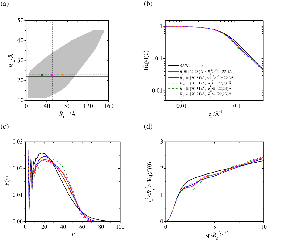
Figure S1: Comparing SAXS properties of the $\epsilon_{\rm p}=-1.0$ homopolymer ensemble and $(R_{\rm g},R_{\rm EE})$ subensembles of $\epsilon_{\rm p}=0$ SAW chains. (a) The homogeneous (homopolymer) ensemble is represented by the gray area corresponding to the overall profile for $\epsilon_{\rm p}=-1.0$ in Fig. 2c of the main text; the $\langle R_{\rm EE}^{2}\rangle^{1/2}$ of this ensemble is indicated by the vertical blue solid line; the notation follows that in Fig. 7 of the main text otherwise. Note that the subensembles marked in (a) and analyzed in (b)–(d) here are sampled from the pure SAW ($\epsilon_{\rm p}=0$) ensemble, not from the $\epsilon_{\rm p}=-1.0$ ensemble.

Aiming to generalize the above analysis to conformations that are more compact or even more open, we have also compared the SAXS signatures of $\epsilon_{\rm p}=0$ SAW subensembles with narrow ranges of $\langle R^{2}_{\rm g}\rangle^{1/2}\approx 22.5$, $18.5$, and $26.5$Å, which are equal, respectively, to the $\langle R^{2}_{\rm g}\rangle^{1/2}$ of the homopolymer ensembles with $\epsilon_{\rm p}=-1.0$, $-1.8$, $+2.0$ (the $R_{\rm g}$–$R_{\rm EE}$ distributions of which are illustrated in Fig. 2). The results of the analysis are documented in Figs. S1–S3 of the Supporting Information. They indicate that while the trend observed in Fig. 7c of a shift of the $P(r)$ peak to higher $r$ values relative to that of the homopolymer ensemble for subensembles with smaller $R_{\rm EE}$ persists in Figs. S1c, S2c, and S3c, none of the subensembles considered—including those with large $R_{\rm EE}$s—has a $P(r)$ that matches closely with the $P(r)$ of the corresponding homopolymer ensembles. Consequently, all of these subensembles entail dimensionless Kratky plots that are quite clearly distinguishable from that of their homopolymer counterparts (Figs. S1d, S2d, and S3d), thus offering examples for which heterogeneous and homogeneous conformational ensembles with the same $\langle R^{2}_{\rm g}\rangle^{1/2}$ can be distinguished by SAXS-determined MFFs alone. At the same time, the observation from Figs. S1–S3 suggests that heterogeneous ensembles constructed as subensembles of homopolymers with different overall compactness may be different even if the subensembles themselves feature the same narrow range of $R_{\rm g}$ and narrow range of $R_{\rm EE}$. This issue will be further explored below.

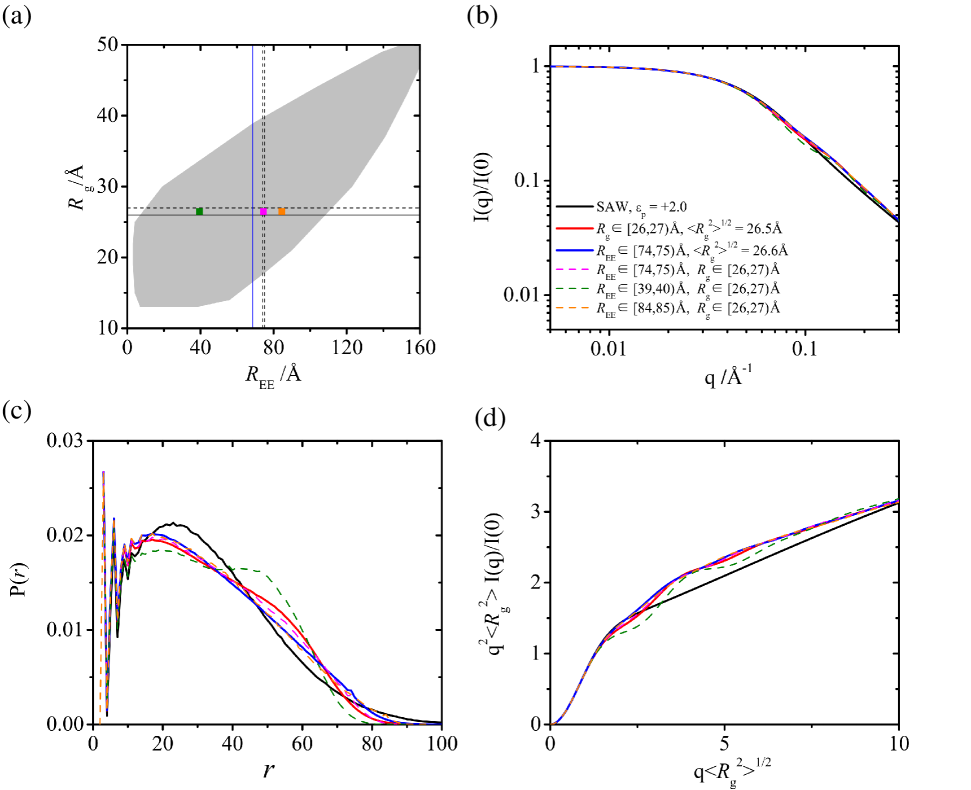
Figure S3: Comparing SAXS properties of the $\epsilon_{\rm p}=+2.0$ homopolymer ensemble and $(R_{\rm g},R_{\rm EE})$ subensembles of $\epsilon_{\rm p}=0$ SAW chains. Same notation as Fig. S1 except the full homogeneous (homopolymer) ensemble here is for $\epsilon_{\rm p}=+2.0$.

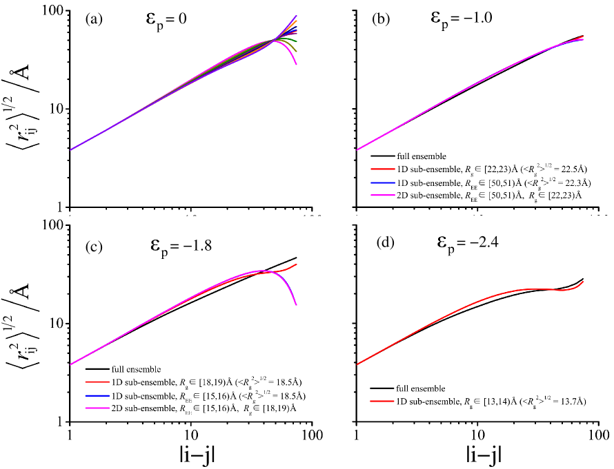
Figure S4: Comparing the $\langle r^{2}_{ij}\rangle^{1/2}$ vs $|i-j|$ relationships of homogeneous (homopolymer) ensembles and heteropolymeric $(R_{\rm g},R_{\rm EE})$ subensembles with essentially identical root-mean-square radii of gyration $\langle R^{2}_{\rm g}\rangle^{1/2}$. (a) Full $\epsilon_{\rm p}=0$ SAW homopolymer ensemble and its subensembles considered in Fig. 8 of the main text. Using the same color code for the lines, the present plot provides their $\langle r^{2}_{ij}\rangle^{1/2}$ as functions of $|i-j|$ over a wider range of $|i-j|$ than that of the main-text figure. (b)–(d) Select full $\epsilon_{\rm p}\neq 0$ homogeneous ensembles (from Fig. 3b of the main text) are compared with select heteropolymeric subensembles sampled from the pure $\epsilon_{\rm p}=0$ SAW homopolymer ensemble (not from an $\epsilon_{\rm p}\neq 0$ ensemble) as specified by the legends. Here, a “1D subensemble” refers to a subensemble with a narrow range of either $R_{\rm g}$ or $R_{\rm EE}$ but not both, and is unrestricted otherwise; whereas a “2D subensemble” is a subensemble with narrow ranges of $R_{\rm g}$ as well as $R_{\rm EE}$.

Root-mean-square of intrachain distance $r_{ij}$ as a function of contour length separation $|i-j|$ are shown for representative subensembles in Fig. S4 of Supporting Information. For subensembles with compact conformational dimensions such as those in Fig. S4d, the $\langle r_{ij}^{2}\rangle^{1/2}$ versus $|i-j|$ relationship is nonlinear, similiar to the corresponding relationships exhibited by the homopolymer ensembles with $\epsilon_{\rm p}\lesssim-2.4$ in Fig. 3b. Indeed, the $\langle r_{ij}^{2}\rangle^{1/2}$ versus $|i-j|$ relationship can be highly nonlinear for heteropolymers,pappu13 ; kings2015 ; huihui2020 in which cases no $\nu$ can be reasonably defined. More recent examples of simulated heteropolymers lacking an approximate $\langle r_{ij}^{2}\rangle^{1/2}\sim|i-j|$ scaling include results shown in Figs. 2 and 4 of ref. (121) and Fig. S3 of ref. (117) even though usage of $\nu$ in lieu of $\langle R^{2}_{\rm g}\rangle$ is advocated in ref. (117). Here, for the subensembles with the same $R_{\rm g}$ as the relatively open $\epsilon_{\rm p}=0$ SAW homopolymers studied in Fig. 7, the $\langle r_{ij}^{2}\rangle^{1/2}$ versus $|i-j|$ plots in Fig. S4a are largely linear except for $|i-j|\approx n=75$, but they do exhibit other, more minor variations despite the subensembles sharing the same $R_{\rm g}$. The divergent behaviors for large $|i-j|$s, which correspond to distances between two ends of the chain, are stemming from the narrow ranges of $R_{\rm EE}$ imposed by the definition of the subensembles. Aside from that, variations are also noticeable for $|i-j|$ $\sim 7$—$40$. A zoomed-in version of the $\langle r_{ij}^{2}\rangle^{1/2}\sim|i-j|^{\nu}$ plots for these subensembles in Fig. 8 indicates that the apparent scaling exponent $\nu$ of the subensembles ranges from $\approx 0.62$ to $0.71$. While these mathematically constructed subensembles are hypothetical as to their physical realizability, they do serve to underscore that for heterogeneous disordered conformational ensembles, the apparent scaling exponent $\nu$ is not necessarily a proxy for $\langle R^{2}_{\rm g}\rangle^{1/2}$, as has been demonstrated recently in combined theoretical/experimental studies of real disordered proteins.raleighPNAS2019 ; raleighBiochem2020 As it stands, $\nu$ is largely a model parameter that is currently not amenable to direct experimental determination. Using such a parameter to replace the experimentally measured $\langle R^{2}_{\rm g}\rangle$ as a descriptor of ensemble properties does not appear to be well advised.

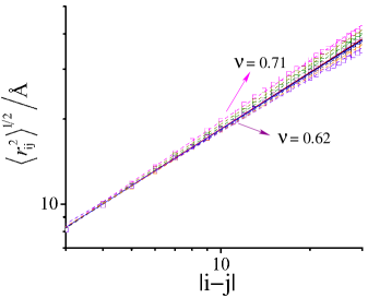
Figure 8: Variation of root-mean-square intrachain monomer-monomer distance $\langle r^{2}_{ij}\rangle^{1/2}$ with sequence separation $|i-j|$ for the SAW homopolymer ensemble and various subensembles in Fig. 7, plotted using the same color code. The maximum and minimum scaling exponents ($\nu$) obtained from the fitted straight lines are indicated.

MFFs of select heterogeneous ensembles with very narrow ranges of ${\bm{R}}_{\bf g}$ and ${\bm{R_{\rm EE}}}$ can be very similar to MFFs of compact homopolymers. Building on the initial results in Figs. S1–S3 (Supporting Information) discussed above, we explore whether and, if so, what heterogeneous ensembles may possess SAXS signatures practically indistinguishable from those of homopolymer ensembles that are more compact or more open than the $\epsilon_{\rm p}=0$ SAW homopolymers. Now, instead of constructing heterogeneous ensembles by selecting from the $\epsilon_{\rm p}=0$ homopolymer conformations as in Figs. S1–S3, we construct heterogeneous ensembles by selecting from the conformations of an $\epsilon_{\rm p}\neq 0$ homopolymer ensemble. Interestingly, among the heterogeneous subensembles constructed in this manner to cover a narrow range of $R_{\rm EE}$ and a narrow range of $R_{\rm g}$ values around the $\langle R^{2}_{\rm g}\rangle^{1/2}$ of the $\epsilon_{\rm p}\neq 0$ homopolymer, some of the heterogeneous subensembles with relatively large $R_{\rm EE}$s can have $P(r)$s very similar to the $P(r)$ of the corresponding homopolymer ensemble with the same $\epsilon_{\rm p}\neq 0$. Consequently, their MFFs are also extremely similar. Examples of such heterogeneous and $\epsilon_{\rm p}\neq 0$ homogeneous ensembles with closely matching dimensionaless Kratky plots are provided in Figs. 9a,b, and c between subensembles with $R_{\rm EE}\approx 70.5$, $65.5$, and $84.5$Å, respectively, and their corresponding homopolymer ensembles with different compactness as specified by $\epsilon_{\rm p}=-1.0$, $-1.8$, and $+2.0$. In line with the $\epsilon_{\rm p}=0$ situation in Fig. 7, the $R_{\rm EE}$ of these subensembles in Figs. 9a–c with homopolymeric SAXS signatures are considerably higher than the $\langle R^{2}_{\rm EE}\rangle^{1/2}\approx 50.5$, $18.5$, and $74.5$Å, respectively, of their corresponding $\epsilon_{\rm p}=-1.0$, $-1.8$, and $+2.0$ homopolymer ensembles. It is instructive to contrast these subensembles of $\epsilon_{\rm p}\neq 0$ homopolymers in Figs. 9a–c exhibiting homopolymeric SAXS signatures with those subensembles with the same narrow $R_{\rm g},R_{\rm EE}$ ranges but constructed from $\epsilon_{\rm p}=0$ chains in Figs. S1–S3 (Supporting Information) that do not exhibit similar SAXS signatures. This observation indicates that MFFs of disordered chains can be sensitive to $\epsilon_{\rm p}$-dependent conformational preferences even when variations in $R_{\rm g}$ and $R_{\rm EE}$ in the ensembles are highly restricted. In any event, the examples of SAXS signature matching in Figs. 9a,b affirm that MFFs of at least some highly heterogeneous ensembles can be practically identical to MFFs of compact homopolymers and therefore these disordered conformational ensembles cannot be distinguished solely by their SAXS spectra.

To facilitate systematic computation and evaluation of MFFs of a large number of heterogeneous ensembles (see below), $\Delta_{\rm Kratky}(1,2)\equiv\int_{0}^{x_{\rm max}}dx|y_{1}(x)-y_{2}(x)|$, where $y=q^{2}\langle R^{2}_{\rm g}\rangle I(q)/I(0)$ and $x=q\langle R^{2}_{\rm g}\rangle^{1/2}$, is hereby defined (Fig. 9d) to quantify the difference in SAXS signature between two conformational ensembles (labeled 1 and 2). As illustrated in Fig. 9d, $\Delta_{\rm Kratky}$ may be viewed as a simple measure of mismatch between two dimensionless Kratky plots. We use $x_{\rm max}=10$ for the present study. Besides the present application, we note that $\Delta_{\rm Kratky}$ may also be useful in future investigations to optimize the match between experimental MFFs and those computed from inferred conformational ensembles.GregJACS2020 ; choy2001

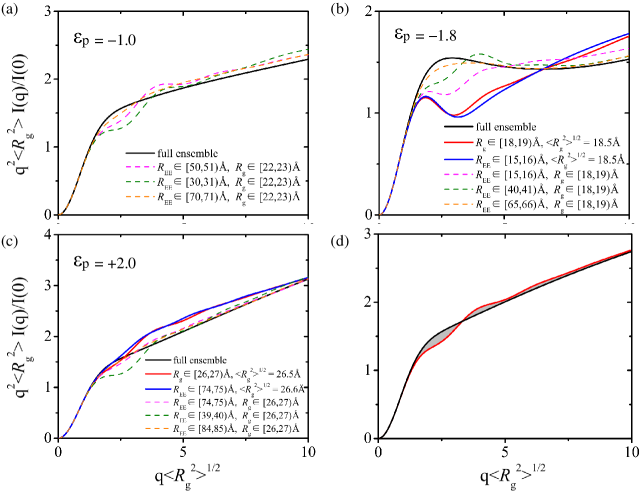
Figure 9: Comparing MFFs of homogeneous and heterogeneous ensembles sharing essentially the same $\langle R^{2}_{\rm g}\rangle^{1/2}$. (a)–(c) Dimensionless Kratky plots (MFFs) of $\epsilon_{\rm p}\neq 0$ homogeneous ensembles are compared with those of subensembles that are subsets of the full ensemble for the given $\epsilon_{\rm p}$ with $R_{\rm g}$ and/or $R_{\rm EE}$ ranges specified by the inset legends. (d) Schematic of a pairwise difference measure for any two dimensionless Kratky plots referred to as $\Delta_{\rm Kratky}$ (see text) and defined as the total area (shaded) between the two plots within a given range of $q\langle R^{2}_{\rm g}\rangle^{1/2}$ (e.g., from $q\langle R^{2}_{\rm g}\rangle^{1/2}=0$ to $10$ as in this depiction). The two Kratky plots shown in (d) are hypothetical and for illustration only. They do not correspond to the simulated Kratky plots in (a)–(c).

MFFs of heterogeneous ensembles with significantly less variation in ${\bm{R}}_{\bf g}$ can still be very similar to MFFs of homopolymeric SAWs. As shown by the above analysis, subensembles defined by narrow ranges of $R_{\rm g}$ and $R_{\rm EE}$ are instrumental—as individual heterogeneous ensembles—in identifying scenarios in which the SAXS signatures of heterogeneous and homogeneous ensembles are clearly distinguishable or remarkably similar, or somewhere in between. In aggregate, these subensembles may be seen as components of a basis set for a “conformational ensemble space” by which other heterogeneous ensembles can be constructed as weighted combinations of component ensembles. In this regard, the homopolymer ensemble is a special case of such an ensemble in which the components are weighted by their fractional populations in the homopolymer ensemble. Adopting this conceptual framework, we now extend our consideration to heterogeneous ensembles, constructed as weighted combinations of $(R_{\rm g},R_{\rm EE})$ subensembles, that encompass a broader variety of conformations. Instead of restricting to narrow ranges $R_{\rm g}$ and $R_{\rm EE}$, nonzero weights are assigned to all conformations in a homopolymer ensemble in the construction of these ensembles. In particular, we are interested in ensembles with a tighter distribution of $R^{2}_{\rm g}$ than the SAW homopolymer ensemble. Such heterogeneous ensembles are apparently less artifical than the individual $(R_{\rm g},R_{\rm EE})$ subensembles. Intuitively, they are physically plausible, especially when the distribution $P(R^{2}_{\rm g})$ of the ensemble is at most moderately tighter than that of a homopolymer ensemble. Conceivably, sequence-dependent effects of IDPs may encode a tighter $P(R^{2}_{\rm g})$ for biological function, as envisioned, e.g., in the proposed polyelectrostatic binding between Sic1 and Cdc4 (ref. (14)). It would be useful, therefore, to ascertain theoretically whether such heterogeneous ensembles are distinguishable from homopolymer ensembles by SAXS-measured MFFs alone or measurements by complementary techniques are needed.

Toward this aim, reweighted ensembles with the same $\langle R^{2}_{\rm g}\rangle$ as the homopolymers but with a narrower distribution of $R^{2}_{\rm g}$ are constructed. Here we let $\delta R^{2}_{\rm g}\equiv R^{2}_{\rm g}-\langle R^{2}_{\rm g}\rangle$ and introduce $\alpha$, $\alpha^{\prime}\geq 0$ as scaling factors for controlling the broadness of the reweighted $R^{2}_{\rm g}$ distribution. For a given homopolymeric $P(R^{2}_{\rm g})$, the reweighted $R^{2}_{\rm g}$ distribution is obtained by the modification $P(R^{2}_{\rm g})\rightarrow$ ${\cal N}_{0}^{-1}\exp[-\alpha(\delta R^{2}_{\rm g})]P(R^{2}_{\rm g})$ for $\delta R^{2}_{\rm g}<0$ and $P(R^{2}_{\rm g})\rightarrow$ ${\cal N}_{0}^{-1}\exp[-\alpha^{\prime}(\delta R^{2}_{\rm g})]P(R^{2}_{\rm g})$ for $\delta R^{2}_{\rm g}>0$ where ${\cal N}_{0}=$ $2\int_{-\infty}^{0}d{\delta}R^{2}_{\rm g}\;\exp[-\alpha(\delta R^{2}_{\rm g})]P(R^{2}_{\rm g})$ is the overall normalization factor for the reweighted (modified) $P(R^{2}_{\rm g})$, and $\alpha^{\prime}$ is related to $\alpha$ by the equation $\int_{-\infty}^{0}d{\delta}R^{2}_{\rm g}\;\exp[-\alpha(\delta R^{2}_{\rm g})]P(R^{2}_{\rm g})$ $=$ ${\cal N}_{0}/2=$ $\int_{0}^{\infty}d{\delta}R^{2}_{\rm g}\;\exp[-\alpha^{\prime}(\delta R^{2}_{\rm g})]P(R^{2}_{\rm g})$, which determines $\alpha^{\prime}$ numerically for any given $\alpha$.

The dimensionless Kratky plots of the SAW ($\epsilon_{\rm p}=0$) homopolymer ensemble and three reweighted ensembles—which are heterogeneous ensembles—are shown in Fig. 10a. Notably, despite the heterogeneous ensembles’ very different $P(R^{2}_{\rm g})$ distributions, ranging from being only slightly narrower than that of the homopolymer ($\alpha=0.001$) to being highly peaked ($\alpha=0.1$, Fig. 10b), their dimensionless Kratky plots are extremely similar (Fig. 10a), exhibiting little variation even in the shoulder regions where considerable variation was observed in Fig. 7d among the dimensionless Kratky plots of the $(R_{\rm g},R_{\rm EE})$ subensembles. Hence, the results in Fig. 10 suggest strongly that certain physically plausible heterogeneous ensembles of disordered proteins with narrower distributions of $R_{\rm g}^{2}$ can hardly be distinguishable by their SAXS signatures from a homopolymer ensemble with the same $\langle R^{2}_{\rm g}\rangle$. We will extend the study of similarly reweighted ensembles to $\epsilon_{\rm p}=-1.0$, $-1.8$, and $+2.0$ below.

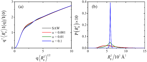
Figure 10: SAXS spectra of conformational ensembles with the same $\langle R^{2}_{\rm g}\rangle$ but different $R^{2}_{\rm g}$ distributions. (a) MFFs (dimensionless Kratky plots) of the homogeneous SAW ($\epsilon_{\rm p}=0$ homopolymer) ensemble and heteropolymeric reweighted ensembles with $\alpha=0.1$, $0.01$, and $0.001$ (the corresponding $\alpha^{\prime}$ values are, respectively, $0.09351$, $0.007153$, and $0.0006099$). (b) $R^{2}_{\rm g}$ distributions of the ensembles in (a) plotted using the same color code. The standard deviations of $R^{2}_{\rm g}$ for the SAW ($\alpha=0$), $\alpha=0.001,$ $0.01$, and $0.1$ distributions are, respectively, 218.7, 205.8, 117.8, and 14.8 Ų, their corresponding square roots are 14.8, 14.3, 10.9, and 3.85 Å.

MFFs of heterogeneous and homogeneous ensembles can be practically identical despite significant differences in ${\bm{R_{\rm EE}}}$, asphericity, and ${\bm{R}}_{\bf g}$ distributions. We have now demonstrated that homopolymer ensembles and certain subensembles defined by very narrow $R_{\rm g},R_{\rm EE}$ ranges and relatively large $R_{\rm EE}$s can lead to essentially indistinguishable dimensionless Kratky plots (Figs. 7d and 9a–c). Separately, high degrees of similarity can also be seen between the dimensionless Kratky plots of homopolymers and those of conformationally more diverse heterogeneous ensembles with slightly to significantly narrower $R^{2}_{\rm g}$ distributions (Fig. 10). In view of these findings, we next consider, in a systematic manner, an extensive set of heterogeneous ensembles with narrower-than-homopolymer distributions of $R_{\rm g}$ similar to those studied in Fig. 10 and also narrower-than-homopolymer distributions of $R_{\rm EE}$ peaking at different $R_{\rm EE}$ values to catalog these heterogeneous ensembles’ SAXS signatures. As such, these heterogeneous ensembles may be viewed as “smeared” versions of the $(R_{\rm g},R_{\rm EE})$ subensembles with very narrow $R_{\rm g},R_{\rm EE}$ ranges. In this regard, these heterogeneous ensembles are intuitively more plausible to be physically encodable by heterpolymeric amino acid sequences and therefore of more immediate relevance to potential experimental situations.

We construct these ensembles by additional reweighting of the above-described reweighted ensembles with narrower $R^{2}_{\rm g}$ distributions, now applied also to chains with $\epsilon_{\rm p}\neq 0$ [$P(R^{2}_{\rm g})$ parameterized by $\epsilon_{\rm p}$ and $\alpha$], to further bias the final ensembles toward a select $R_{\rm EE}$ value. Let $P(R^{2}_{\rm g},R_{\rm EE})$ be the fractional population density with square radius of gyration $R^{2}_{\rm g}$ and end-to-end distance $R_{\rm EE}$. By definition, the above $\alpha$-dependent reweighted $P(R^{2}_{\rm g})$ may be written as an integral over $P(R^{2}_{\rm g},R_{\rm EE})$, viz.,

$$P(R^{2}_{\rm g})=\int_{0}^{\infty}dR_{\rm EE}\;P(R^{2}_{\rm g},R_{\rm EE})\;.$$ (3)

We now reweight each $P(R^{2}_{\rm g},R_{\rm EE})$ as follows:

$$P(R^{2}_{\rm g},R_{\rm EE})\rightarrow{\cal N}(R_{\rm g},\gamma,R^{0}_{\rm EE})^{-1}P(R^{2}_{\rm g},R_{\rm EE})\exp[-\gamma(R_{\rm EE}-R^{0}_{\rm EE})^{2}]\;,$$ (4)

where the normalization factor ${\cal N}(R_{\rm g},\gamma,R^{0}_{\rm EE})$, defined by

$$\int_{0}^{\infty}dR_{\rm EE}P(R^{2}_{\rm g},R_{\rm EE})\exp[-\gamma(R_{\rm EE}-R^{0}_{\rm EE})^{2}]={\cal N}(R_{\rm g},\gamma,R^{0}_{\rm EE})\int_{0}^{\infty}dR_{\rm EE}P(R^{2}_{\rm g},R_{\rm EE})\;,$$ (5)

preserves the weight of each individual $R^{2}_{\rm g}$ value, and therefore the overall $\langle R^{2}_{\rm g}\rangle$ of the reweighted ensemble remains the same as that of the original ensemble. In Eqs. 4 and 5, $R^{0}_{\rm EE}$ is an input parameter, a reference value of $R_{\rm EE}$ toward which the ensemble is biased to a degree parameterized by $\gamma$. It should be noted that the actual $\langle R_{\rm EE}\rangle$ or $\langle R^{2}_{\rm EE}\rangle^{1/2}$ of the final reweighted ensemble depends on $\alpha$, $\gamma$ as well as the value of $R^{2}_{\rm g}$ and is therefore not expected to be exactly equal to $R^{0}_{\rm EE}$.

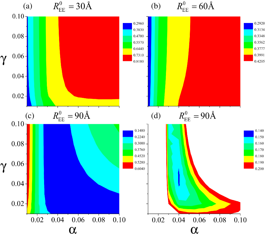
Figure S5: Extensive cataloging of SAXS properties of reweighted heterogeneous ensembles. $\Delta_{\rm Kratky}$ between $(R^{0}_{\rm EE},\alpha,\gamma)$-defined reweighted ensembles (see main text for details) and the homogeneous SAW ($\epsilon_{\rm p}=0$) homopolymer ensemble is computed for three select $R^{0}_{\rm EE}$ values: (a) 30 Å, (b) 60 Å, and (c,d) 90 Å, each for a $10\times 10$ grid ($0.01$ increments) of $\alpha,\gamma$ values. Shown here (a–d) are the resulting contour plots, with (c) and (d) for the same $R^{0}_{\rm EE}=90$ Å data plotted with different contour increments. For the systems considered, the $(R^{0}_{\rm EE}/{\rm\AA},\alpha,\gamma)$ at the minimum $\Delta_{\rm Kratky}$ values encountered (approximate minimum $\Delta_{\rm Kratky}$ in curly brackets) are as follows: (30, 0.01, 0.01) {0.30}, (60, 0.01, 0.1) {0.30}, and (90, 0.04, 0.05) {0.14}. Similar analyses are performed for $\epsilon_{\rm p}=-1.0$, $-1.8$, and $+2.0$ (contour plots not shown), the resulting minimum-$\Delta_{\rm Kratky}$ $(R^{0}_{\rm EE}/{\rm\AA},\alpha,\gamma)$ parameters and approximate minimum $\Delta_{\rm Kratky}$ values are (same notation as above): For $\epsilon_{\rm p}=-1.0$, (22.7, 0.01, 0.01) {0.36}, (52.7, 0.01, 0.01) {0.31}, and (82.7, 0.06, 0.06) {0.14}; for $\epsilon_{\rm p}=-1.8$, (11.8, 0.02, 0.01) {0.30}, (41.8, 0.01, 0.01) {0.31}, and (71.8, 0.07, 0.03) {0.16}; and for $\epsilon_{\rm p}=+2.0$, (35.0, 0.01, 0.01) {0.30}, (65.0, 0.01, 0.01) {0.30}, and (95.0, 0.04, 0.1) {0.21}.

Using the MFF difference measure $\Delta_{\rm Kratky}$ defined above (Fig. 9d), we have conducted an extensive exploration of the $\alpha,\gamma,R^{0}_{\rm EE}$ parameter space to identify heterogeneous ensembles with MFFs closely matching those of homopolymers. Because it is combinatorically impractical to examine all three parameters exhaustively, we focus on several representative $R^{0}_{\rm EE}$ values. We do so by first examining $\Delta_{\rm Kratky}$ between homopolymer ensembles and an extensive set of heterogeneous ensembles parametrized by combinations of $\alpha,\gamma$ values for $R^{0}_{\rm EE}=$ $30$, $60$, and $90$Å. As shown in Fig. S5 of Supporting Information, the results of this calculation suggest that ensembles with $R^{0}_{\rm EE}=90$Å are more likely to lead to small $\Delta_{\rm Kratky}$, especially when putative optimal values for $\gamma\approx 0.05$, $0.06$, $0.03$, and $0.1$ that minimize $\Delta_{\rm Kratky}$ are chosen, respectively, for chains with intrachain interaction $\epsilon_{\rm p}=0$, $-1.0$, $-1.8$, and $+2.0$.

We then proceed to explore the $\alpha,R^{0}_{\rm EE}$ parameter space while using these putative optimal $\gamma$ values as given (Fig. 11). The variations of the resulting $\Delta_{\rm Kratky}$ between homopolymer ensembles and the heterogeneous ensembles as functions of $\alpha$ and $R^{0}_{\rm EE}$ are depicted by the contour/heat plots in Figs. 11a–d. Interestingly, while minimal $\Delta_{\rm Kratky}$ is found in a region of relatively large $R^{0}_{\rm EE}$ $\sim 70$–$100$Å in every case studied here (most lightly shaded region in Figs. 11a–d)—as one might expected because selection of the $\gamma$ parameters used in Fig. 11 is based on ensembles with $R^{0}_{\rm EE}=90$Å in Fig. S5, a second minimal-$\Delta_{\rm Kratky}$ region is also observed in Fig. 11c around $R^{0}_{\rm EE}\approx 30$Å and $\alpha\approx 0.01$.

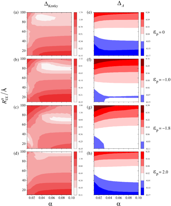
Figure 11: Variation of SAXS behaviors and conformational asphericity among heteropolymeric ensembles with the same $\langle R^{2}_{\rm g}\rangle$. (a)–(d) $\Delta_{\rm Kratky}$ and (e)–(h) difference in average asphericity, $\Delta_{A}$, between heteropolymeric $(R^{0}_{\rm EE},\alpha,\gamma)$-defined reweighted ensembles ($\gamma=0.05$, $0.06$, $0.03$, and $0.1$, respectively, for $\epsilon_{\rm p}=0$, $-1.0$, $-1.8$, and $+2.0$) and the homogeneous ensemble for the given $\epsilon_{\rm p}$ values are computed for a $10\times 10$ grid of ($R^{0}_{\rm EE},\alpha$) values to produce each of the contour plots. $\Delta_{A}$ is the average asphericity of the heteropolymeric ensemble minus that of the homogeneous ensemble.

To quantify the structural differences between the reweighted heterogeneous ensembles constructed for chains with different intrachain interaction energy $\epsilon_{\rm p}$ with their corresponding homopolymer ensemble, we compute the asphericitykuhn1934 for each chain conformation, defined asRudnick1986

$$A\equiv 1-\frac{3(\lambda_{1}\lambda_{2}+\lambda_{1}\lambda_{3}+\lambda_{2}\lambda_{3})}{(\lambda_{1}+\lambda_{2}+\lambda_{3})^{2}}\;,$$ (6)

where $\lambda_{1},\lambda_{2},\lambda_{3}$ (all $\geq 0$) are the eigenvalues of the gyration tensor $S_{\mu\nu}\equiv n^{-1}\sum_{i=1}^{n}({\bf R}_{i}-{\bf R}_{\rm cm})_{\mu}({\bf R}_{i}-{\bf R}_{\rm cm})_{\nu}$, where $\mu,\nu=1,2,3$ label the Cartesian axes (the $\nu$ index here should not be confused with the exponent $\nu$ for pair distance scaling), and $R_{\rm g}^{2}=\lambda_{1}+\lambda_{2}+\lambda_{3}$. The asphericity quantity $A$ has been used to analyze folded and disordered states of proteins,DT2004 ; Rohit2006 including recent theoretical applications to better understand smFRET and SAXS signatures of disordered proteins.Songetal2015 ; DT2019 Here we determine the average asphericity, $\langle A\rangle$, for each ensemble of interest by averaging $A$ over the (weighted) conformations in the ensemble and, as measure for one aspect of structural differences between a heterogeneous ensemble and a homopolymer ensemble, we define $\Delta_{A}$ as the difference between $\langle A\rangle$ of a heterogeneous ensemble and that of a homopolymer ensemble. The variations of $\Delta_{A}$ among the reweighted heterogeneous ensembles as functions of $\alpha$ and $R^{0}_{\rm EE}$ are depicted by the contour/heat plots in Figs. 11e–h.

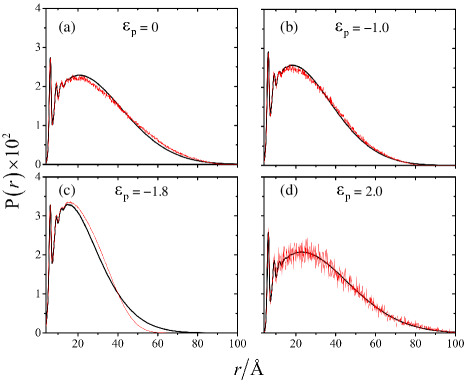
Figure 12: Homogeneous and heterogeneous ensembles can have essentially identical distributions of intrachain monomer-monomer distances. $P(r)$s are shown for the homogeneous ensembles (black curves) and the heteropolymeric reweighted ensembles with minimized $\Delta_{\rm Kratky}$ deduced from Fig. 11 (red curves). The reweighting parameters $(R^{0}_{\rm EE}/{\rm\AA},\alpha,\gamma)$ for minimum $\Delta_{\rm Kratky}$ are: (a) (90.0, 0.04, 0.05), (b) (80.0, 0.08, 0.06), (c) (30.0, 0.01, 0.03), and (d) (110.0, 0.1, 0.1).

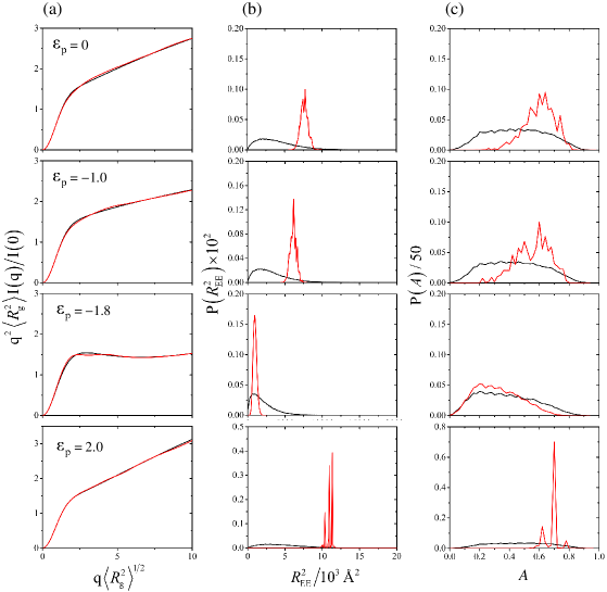
Figure 13: Drastically different disordered conformational ensembles can lead to essentially identical MFFs. (a) Dimensionless Kratky plots (MFFs), (b) distributions of square end-to-end distances $R^{2}_{\rm EE}$, and (c) distributions of conformational asphericity $A$ are shown for the homogeneous ensembles (black curves) and heteropolymeric minimum-$\Delta_{\rm Kratky}$ reweighted ensembles (red curves) in Fig. 12. The standard deviation of the $R^{2}_{\rm g}$ distribution (in units of Ų), $\langle R_{\rm EE}^{2}\rangle^{1/2}/{\rm\AA}$, and $\langle A\rangle$ for the homogeneous $\epsilon_{\rm p}=0$ ensemble are 218.7, 62.5, 0.461, respectively; whereas the corresponding values for the $\epsilon_{\rm p}=0$ minimum-$\Delta_{\rm Kratky}$ ensemble are 42.8, 87.3, 0.610. For $\epsilon_{\rm p}=-1.0$, the corresponding numbers are 190.1, 56.0, 0.442; 19.0, 78.1, 0.566. For $\epsilon_{\rm p}=-1.8$: 149.8, 45.1, 0.386; 70.1, 31.1, 0.331, and for $\epsilon_{\rm p}=+2.0$: 248.8, 68.6, 0.473; 31.9, 105.0, 0.696. The $10^{2}$ (b) and $1/50$ (c) in the vertical variables are normalization factors.

Figs. 11a–d show that there are low-$\Delta_{\rm Kratky}$ regions of considerable extent in $(\alpha,R^{0}_{\rm EE})$ parameter space, but these regions do not coincide with the low-$\Delta_{A}$ white regions in Figs. 11e–h. This observation indicates that there are a wide variety of heterogeneous ensembles with conformational properties significantly different from those of homopolymers but nonetheless possess SAXS signatures essentially indistinguishable from those of homopolymers. Examples of how the pair distance distribution function $P(r)$ of some of these heterogeneous ensembles with minimal $\Delta_{\rm Kratky}$ match closely with the $P(r)$ of homopolymer ensembles are provided in Fig. 12. As far as MFFs are concerned, it follows that the dimensionless Kratky plots of the four example heterogeneous ensembles in Figs. 12a–d, constructed from chains with intrachain interaction energy $\epsilon_{\rm p}=0$, $-1.0$, $-1.8$, and $+2.0$, and therefore are of different conformational compactness characterized by $\langle R^{2}_{\rm g}\rangle^{1/2}=24.4$, $22.2$, $18.5$, and $26.5$Å, respectively, are hardly distinguishable from the dimensionless Kratky plots of their homopolymeric counterparts (Fig. 13a). Despite the near-coincidence of their SAXS signatures of these pairs of heterogeneous and homogeneous ensembles, their conformational properties are drastically different, as can be seen by their very different distributions of mean square end-to-end distance (Fig. 13b) and average asphericity (Fig. 13c). Interestingly, among the four examples highlighted, the average asphericities of the heterogeneous and homogeneous ensembles are least dissimilar for the $\epsilon_{\rm p}=-1.8$ case ($\langle R^{2}_{\rm g}\rangle^{1/2}=18.5$, Fig. 13, third row from top). This feature may be a result of contraints imposed by the overall conformational compactness, or it may be related to our choice of this particular heterogeneous ensemble with an $R_{\rm EE}^{2}$ distribution peak that coincides approximately with that of the homopolymer ensemble, though the $R_{\rm EE}^{2}$ distribution itself is much narrower for the heterogeneous ensemble than for the homopolymer ensemble. In any event, the above extensive cataloging of SAXS signatures of heterogeneous ensembles (Fig. 11) and the explicit examples in Figs. 12 and 13 demonstrate that, across conformational ensembles of different overall compactness, certain heterogeneous ensembles with conformational properties dramatically different from those of homopolymers can nonetheless exhibit essentially identical SAXS signatures as homopolymers.

Approximate analytical theory for sequence-dependent MFFs of disordered heteropolymers. The heterogeneous ensembles considered above are tools for logically delineating the information content of SAXS signatures. To serve as examples and counterexamples, it suffices to define these ensembles mathematically, as long as the ensembles are in principle physically realizable, without demonstrating how the presumed protein ensembles might be encoded exactly by amino acid sequences. Nonetheless, it is intuitively plausible that disordered protein ensembles similar to some—though not all—of these constructs, such as the reweighted ensembles encompassing diverse conformations but with distributions of $R^{2}_{\rm g}$ somewhat narrower than those of homopolymers (Fig. 10), may be encodable by specific amino acid sequences. Given the current inadequate understanding of the physical interactions governing conformational properties of disordered proteins,cosb15 few insights, if any, exist as to the encodability of heterogeneous disordered protein ensembles, i.e., there is very little knowledge about what ensembles are physically realizable and what ensembles are not. In this light, while a recent analysis of computed MFFs of heteropolymers with hydrophobicity-like interactions led the authors to conclude that “$R_{\rm g}$ and $R_{\rm EE}$ remain coupled even for heteropolymers”,tobinPNAS2019 it should be noted that their study covered only a limited regime of heteropolymeric interactions, leaving the likely vast possibilities of disordered conformational heterogeneity allowable by polypeptide sequences unsurveyed. Here we take a rudimentary step to further explore these possibilities by developing an extension of the perturbative techniques in polymer theory for treating excluded volume effectsfixman1955 ; fixman1962a ; fixman1962b ; Edwards1965 ; tanaka1966 ; ohta81 ; Freedbook ; ohta82 ; muthu84 ; chanJCP89 ; chanJCP90 to incorporate heterogeneous pairwise intrachain interactions. Although our analytical formulation is restricted to contact-like interactions with a short spatial range and thus subtle effects of polypeptide interactions cannot be addressed, results below from this computationally efficient approach are instructive in offering a glimpse of how various properties of heterogeneous disordered ensembles—including decoupling of $R_{\rm g}$ and $R_{\rm EE}$ in some cases—might be encoded.

Our analytical formulation is based on the path-integral representation of the polymer partition function

$${\cal Q}(N,\{{\tilde{v}}\})=\int[{\cal D}{\bf R}]\*{\rm e}^{-{\cal H}(N,\{{\tilde{v}}\},\{{\bf R}\})}\;\;,$$ (7)

where $N$ is the total contour length of the polymer and ${\bf R}(\tau)$ is the spatial position of the point labeled by the contour length variable $\tau$ along the polymer. If a bond connecting two monomer beads is identified with a chain segment of length $l$, the total number of beads in each chain modeled by Eq. 7 is equal to $n=N/l+1$. For notational convenience, $l$ is set to unity ($l=1$) unless specified otherwise. The Hamiltonian ${\cal H}$ is given by

$${\cal H}(N,\{{\tilde{v}}\},\{{\bf R}\})=\frac{1}{2}\int_{0}^{N}d\tau\;\Bigl{|}\frac{d{\bf R}(\tau)}{{d\tau}}\Bigr{|}^{2}+\int_{a}^{N}d\tau\int_{0}^{\tau-a}d\tau^{\prime}\;{\tilde{v}}(\tau,\tau^{\prime})\delta[{\bf R}(\tau)-{\bf R}(\tau^{\prime})]\;,$$ (8)

where ${\tilde{v}}(\tau,\tau^{\prime})$ is the pairwise interaction energy between the points labeled by $\tau$ and $\tau^{\prime}$ along the polymer chain, and $a\sim 1$ is a cutoff in contour length to remove unphysical self interaction of any chain segment with itself. In general, the energy function ${\tilde{v}}(\tau,\tau^{\prime})$ depends on $\tau,\tau^{\prime}$ and thus the formulation describes a heteropolymer. In the special case when ${\tilde{v}}(\tau,\tau^{\prime})$ $={\tilde{v}}_{0}>0$, i.e., when $\tilde{v}$ is independent of $\tau$ and $\tau^{\prime}$, Eqs. 7 and 8 reduce to those for a homopolymer with uniform excluded volume interactions [see, e.g., Eqs. (5.1) and (5.2) of ref. (108) and Eqs. (4.1) and (4.2) of ref. (109)]. It should also be noted that although we allow individual pairwise interactions in Eq. 8 to be neutral, attractive or repulsive, for simplicity, we do not employ a three-body repulsion term (as in some other analytical formulations, see, e.g., ref. (121)) to account for excluded volume when ${\tilde{v}}$ is attractive in the present perturbative treatment.

Diagrammatic perturbation expansions in the present heteropolymer formulation proceed largely along the description in ref. (108) except $v_{0}$ in this reference is now replaced by ${\tilde{v}}(\tau,\tau^{\prime})$ which is then placed inside the $\int d\tau\int d\tau^{\prime}$ integrals as a factor of the integrand. As well, the ${\bf c}(\tau)=\sqrt{d}{\bf R}(\tau)$ rescaling of the spatial coordinates in ref. (108) is not applied here because it offers no advantage for our present applications which are all for $d=3$ spatial dimensions. As a result, the propagator given by Eq. (5.10) of ref. (108) is now replaced by $(3/2\pi)^{3/2}(1/|\tau-\tau^{\prime}|)^{3/2}\exp[-3|{\bf R}-{\bf R}^{\prime}|^{2}/(2|\tau-\tau^{\prime}|)]$. To simplify the expressions to be presented below, we define $v(\tau,\tau^{\prime})$ $\equiv$ $(3/2\pi)^{3/2}{\tilde{v}}(\tau,\tau^{\prime})$ and $v_{0}\equiv(3/2\pi)^{3/2}{\tilde{v}}_{0}$. After all these notational modifications are taken into account, the “$v_{0}$” in ref. (109) is seen to be equivalent to $(2\pi)^{3/2}v_{0}$ in the present formulation.

Figure 14: Diagrams for perturbative calculations of scattering intensities for heteropolymers. $v_{ij}$ is the interaction energy between contour positions $\tau_{i}$ and $\tau_{j}$. Contour positions $s$ and $s^{\prime}$ at spatial positions ${\bf R}$ and ${\bf R}^{\prime}$ (connected by a dashed line) are associated with the scattering vector ${\bf q}$.

In the present notation, the standard perturbative formula for mean square end-to-end distancefixman1955 ; muthu84 is now generalized to

$$\langle R_{\rm EE}^{2}\rangle=N+\int_{a}^{N}d\tau_{j}\int_{0}^{\tau_{j}-a}d\tau_{i}\frac{{v}_{ij}}{\sqrt{\Delta\tau_{ij}}}+O(v_{ij}^{2})\;$$ (9)

for heteropolymer, where $\Delta\tau_{ij}\equiv\tau_{j}-\tau_{i}$ is the contact orderchanJCP89 ; chanJCP90 of the $\tau_{i},\tau_{j}$ contact, and $v_{ij}=v(\tau_{i},\tau_{j})$. For $v_{ij}=v_{0}$, i.e., for the special case in which the chain is a homopolymer, the above expression reduces to

$$\langle R_{\rm EE}^{2}\rangle=N\biggl{\{}1+v_{0}\biggl{[}\frac{4}{3}\sqrt{N}-\biggl{(}2\sqrt{a}-\frac{2a^{3/2}}{3N}\biggr{)}\biggr{]}\biggr{\}}+O(v_{0}^{2})\;,$$ (10)

as in refs. (99) and (107). For heteropolymers with discrete sequences, we replace the integral in Eq. 9 by summing over a discrete interaction matrix $v_{ij}$—which may be viewed as containing the net energetic effects of “hard-core” excluded volume repulsions and short-spatial-ranged sequence-dependent attractive or repulsive interactions, viz.,

$$\langle R_{\rm EE}^{2}\rangle=N+\sum_{j=2}^{n}\sum_{i=1}^{j-1}\frac{v_{ij}}{\sqrt{\Delta_{ij}}}+O(v_{ij}^{2})\;$$ (11)

where $\Delta_{ij}\equiv j-i$, and $a=1$ is used for the double summations here in Eq. 11.

Application of the above-described perturbative formalism to the Feynman-type diagrams in Fig. 14 for heteropolymer scattering intensities (which correspond to the six diagrams in Fig. 1 of Ohta etal.ohta82 for homopolymer scattering intensities) leads to the following perturbative expression for the scattering intensity:

$$I(q) = \frac{2}{\alpha}\biggl{[}N+\frac{1}{\alpha}\Bigl{(}e^{-\alpha N}-1\Bigr{)}\biggr{]}$$

$$-2\int_{a}^{N}d\tau_{j}\int_{0}^{\tau_{j}-a}d\tau_{i}\frac{v_{ij}}{\Delta\tau_{ij}^{3/2}}\Biggl{\{}\frac{1}{\alpha}\biggl{[}N-\Delta\tau_{ij}+\frac{1}{\alpha}\Bigl{(}e^{-\alpha(N-\Delta\tau_{ij})}-1\Bigr{)}\biggr{]}$$

$$\quad+\Delta\tau_{ij}\biggl{[}\frac{1}{\alpha}\biggl{(}2-e^{-\alpha\tau_{i}}-e^{-\alpha(N-\tau_{j})}\biggr{)}+\frac{\Delta\tau_{ij}}{2}\biggr{]}{\cal F}\Bigl{(}\frac{\sqrt{\alpha\Delta\tau_{ij}}}{2}\Bigr{)}\Biggr{\}}+O(v_{ij}^{2})\;$$

where $\alpha\equiv q^{2}/6$, and

$${\cal F}(z)\equiv\frac{e^{-z^{2}}}{z}\int_{0}^{z}dt\;e^{t^{2}}\;$$ (13)

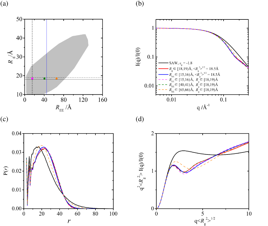
Figure S2: Comparing SAXS properties of the $\epsilon_{\rm p}=-1.8$ homopolymer ensemble and $(R_{\rm g},R_{\rm EE})$ subensembles of $\epsilon_{\rm p}=0$ SAW chains. Same notation as Fig. S1 except the full homogeneous (homopolymer) ensemble here is for $\epsilon_{\rm p}=-1.8$.

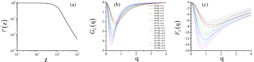
Figure S6: Useful mathematical functions in the present perturbative treatment of scattering intensities. (a) ${\cal F}(z)$ is the function defined in Eq. 13 of the main text. (b) $G_{2}(q)$ is the $G_{2}(N,q;a)$ function in Eq. 28 of the main text, shown here for a variety of $N$ and $a$ values as specified by the inset legend. (c) $F_{2}(q)$ is the $F_{2}(N,q;a)$ function in Eq. 30 of the main text for the same set of $N$ and $a$ values in (b) plotted in the same line styles as those in (b).

is plotted in Fig. S6a of the Supporting Information. We have verified by a rather involved algebraic comparison of the expressions in Eqs. (LABEL:Iq-eq0) and (13) for the $v_{ij}=v_{0}$ special case of homopolymers against the results provided by Eqs. (3.3)–(3.8) in Ohta et al.ohta82 that our first-order perturbative results for $I(q)$ are consistent with theirs except for several likely typographical errors in ref. (106), as described in the Supporting Information of the present article. In this regard, we should also note that the subject matter and goals of the two efforts are different: whereas ref. (106) studies universal homopolymeric behaviors in the limit of infinite chain length through renormalization group analysisoono_ren81-1 (see the “RN” Kratky plot in Fig. S2A of ref. (93) and the $I(x)$ curve in Fig. 2 of ref. (106)), the main focus of the present work is on sequence-specific properties of finite-length heteropolymers.

Proceeding now from Eq. LABEL:Iq-eq0 above, as $q\rightarrow 0$, i.e., in the $\alpha\rightarrow 0$ limit, the expression in Eq. LABEL:Iq-eq0 becomes

$$I(0)=N^{2}\biggl{[}1-\int_{a}^{N}d\tau_{j}\int_{0}^{\tau_{j}-a}d\tau_{i}\frac{v_{ij}}{\Delta\tau_{ij}^{3/2}}\biggr{]}+O(v_{ij}^{2})\;$$ (14)

because ${\cal F}(z)=1-2z^{2}/3+4z^{4}/15-8z^{6}/105+O(z^{8})$, thus ${\cal F}(\sqrt{\alpha\Delta\tau_{ij}}/2)=1-\alpha\Delta\tau_{ij}/6+\alpha^{2}(\Delta\tau_{ij})^{2}/60+O(\alpha^{3})$ and hence $\lim_{\alpha\to 0}{\cal F}(\sqrt{\alpha\Delta\tau_{ij}}/2)=1$. It follows that

$$\frac{I(q)}{I(0)} = \frac{2}{\alpha N}\biggl{[}1+\frac{1}{\alpha N}\Bigl{(}e^{-\alpha N}-1\Bigr{)}\biggr{]}$$ (15)

$$-2\int_{a}^{N}d\tau_{j}\int_{0}^{\tau_{j}-a}d\tau_{i}\frac{v_{ij}}{\Delta\tau_{ij}^{3/2}}\Biggl{\{}\frac{1}{\alpha N}\Bigl{[}-\frac{\Delta\tau_{ij}}{N}+\frac{1}{\alpha N}\Bigl{(}e^{-\alpha(N-\Delta\tau_{ij})}-e^{-\alpha N}\Bigr{)}\Bigr{]}$$

$$\quad+\frac{\Delta\tau_{ij}}{N}\biggl{[}\frac{1}{\alpha N}\biggl{(}2-e^{-\alpha\tau_{i}}-e^{-\alpha(N-\tau_{j})}\biggr{)}+\frac{\Delta\tau_{ij}}{2N}\biggr{]}{\cal F}\Bigl{(}\frac{\sqrt{\alpha\Delta\tau_{ij}}}{2}\Bigr{)}\Biggr{\}}+O(v_{ij}^{2}).$$

Using the standard formula for Guinier’s approximation,AndoChemRev2017

$$\langle R_{\rm g}^{2}\rangle=-3\frac{d}{dq^{2}}[I(q)/I(0)]|_{q=0}=-\frac{1}{2}\frac{d}{d\alpha}[I(q)/I(0)]|_{\alpha=0}$$ (16)

as well as the expansion $d{\cal F}(z)/dz=-4z/3+16z^{3}/15-16z^{5}/35+O(z^{7})$ and thus $d{\cal F}(\sqrt{\alpha\Delta\tau_{ij}}/2)/d\alpha=-\Delta\tau_{ij}/6+\alpha(\Delta\tau_{ij})^{2}/30+O(\alpha^{2})$ and therefore $\lim_{\alpha\to 0}d{\cal F}(\sqrt{\alpha\Delta\tau_{ij}}/2)/d\alpha=-\Delta\tau_{ij}/6$, we obtain, in (implicit) units of $l^{2}$:

$$\langle R^{2}_{\rm g}\rangle = \frac{N}{6}-\int_{a}^{N}d\tau_{j}\int_{0}^{\tau_{j}-a}d\tau_{i}\frac{v_{ij}}{\Delta\tau_{ij}^{3/2}}\biggl{\{}\frac{\Delta\tau_{ij}}{2}\biggl{[}\frac{\tau_{i}^{2}+(N-\tau_{j})^{2}}{N^{2}}-1\biggr{]}+\frac{2\Delta\tau_{ij}^{2}}{3N}-\frac{\Delta\tau_{ij}^{3}}{4N^{2}}\biggr{\}}$$ (17)

$$+O(v_{ij}^{2})\;.$$

For the special case of homopolymer, $v_{ij}=v_{0}$, and this expression reduces to

$$\langle R_{\rm g}^{2}\rangle=\frac{N}{6}\biggl{\{}1+v_{0}\biggl{[}\frac{134}{105}\sqrt{N}-\biggl{(}2\sqrt{a}-\frac{2a^{3/2}}{3N}+\frac{a^{5/2}}{5N^{2}}+\frac{a^{7/2}}{7N^{3}}\biggr{)}\biggr{]}\biggr{\}}+O(v_{0}^{2})\;,$$ (18)

which is consistent with the result of Fixman.fixman1955 For heteropolymers, combining Eq. 9 with Eq. 17 yields

$$\frac{\langle R^{2}_{\rm g}\rangle}{\langle R^{2}_{\rm EE}\rangle} = \frac{1}{6}-\int_{a}^{N}d\tau_{j}\int_{0}^{\tau_{j}-a}d\tau_{i}\frac{v_{ij}}{\Delta\tau_{ij}^{3/2}}\biggl{\{}\frac{\Delta\tau_{ij}}{2N}\biggl{[}\frac{\tau_{i}^{2}+(N-\tau_{j})^{2}}{N^{2}}+1\biggr{]}+\frac{2\Delta\tau_{ij}^{2}}{3N^{2}}-\frac{\Delta\tau_{ij}^{3}}{4N^{3}}\biggr{\}}$$ (19)

$$+O(v_{ij}^{2})\;.$$

The corresponding expression for homopolymers is obtained by combining Eq. 10 and Eq. 18:

$$\frac{\langle R_{\rm g}^{2}\rangle}{\langle R_{\rm EE}^{2}\rangle}=\frac{1}{6}\biggl{\{}1-v_{0}\biggl{[}\frac{2}{35}\sqrt{N}+\biggl{(}\frac{a^{5/2}}{5N^{2}}+\frac{a^{7/2}}{7N^{3}}\biggr{)}\biggr{]}\biggr{\}}+O(v_{0}^{2})\>.$$ (20)

For heteropolymers with discrete sequences, the integrals in Eq. 15 for $I(q)/I(0)$, Eq. 17 for $\langle R^{2}_{\rm g}\rangle$, and Eq. 19 for $\langle R^{2}_{\rm g}\rangle/\langle R^{2}_{\rm EE}\rangle$ are replaced by summmations with a discrete pairwise interaction matrix $v_{ij}$ that replaces the $v_{ij}=v(\tau_{i},\tau_{j})$ in the continuum, viz.,

$$\int_{a}^{N}d\tau_{j}\int_{0}^{\tau_{j}-a}d\tau_{i}\longleftrightarrow\sum_{j=a+1}^{n}\sum_{i=1}^{j-a}\;,$$ (21)

where, in most cases, we take $a=1$ as in Eq. 11 for $\langle R_{\rm EE}^{2}\rangle$. Practically, the same discretization is also used for numerical calculations of $I(q)/I(0)$ for homopolymers when $v_{ij}=v_{0}$. In general, it follows from Eq. 15 that

$$\frac{I(q)}{I(0)}=\biggl{[}\frac{I(q)}{I(0)}\biggr{]}_{0}+{\widetilde{G}}_{2}(N,\{v_{ij}\},q;a)+O(v_{ij}^{2})\;,$$ (22)

whereohta81

$$\biggl{[}\frac{I(q)}{I(0)}\biggr{]}_{0}=\frac{2}{\alpha N}\biggl{[}1+\frac{1}{\alpha N}\Bigl{(}e^{-\alpha N}-1\Bigr{)}\biggr{]}\;$$ (23)

follows from the $P(r)=(8\pi r^{2}/N^{2})\int_{0}^{N}dx(N-x)(3/2\pi x)^{3/2}\exp(-3r^{2}/2x)$ pair distance distribution function for Gaussian chains, and

$${\widetilde{G}}_{2}(N,\{v_{ij}\},q;a) \equiv -\frac{2}{N^{2}}\sum_{j=a+1}^{n}\sum_{i=1}^{j-a}\frac{v_{ij}}{\Delta_{ij}^{3/2}}\Biggl{\{}\frac{1}{\alpha}\biggl{[}-\Delta_{ij}+\frac{1}{\alpha}\Bigl{(}e^{-\alpha(N-\Delta\tau_{ij})}-e^{-\alpha N}\Bigr{)}\biggr{]}$$ (24)

$$\quad+\Delta_{ij}\biggl{[}\frac{1}{\alpha}\biggl{(}2-e^{-\alpha i}-e^{-\alpha(N-j)}\biggr{)}+\frac{\Delta_{ij}}{2}\biggr{]}{\cal F}\Bigl{(}\frac{\sqrt{\alpha\Delta_{ij}}}{2}\Bigr{)}\Biggr{\}}\;$$

in the discretized form. The continuum form for ${\widetilde{G}}_{2}(N,\{v_{ij}\},q;a)$ is readily obtainable by replacing the double summations by the double integrals in Eq. 24 in accordance with the correspondence specified in Eq. 21. To show $I(q)/I(0)$ in a logarithmic scale, which is a common practice as in Figs. 4a and 7b, we use the standard expansion of $\ln(1+x)=x+O(x^{2})$ to recast Eq. 22 as

$$\ln\biggl{[}\frac{I(q)}{I(0)}\biggr{]}=\biggl{[}\frac{I(q)}{I(0)}\biggr{]}_{0}+{\widetilde{F}}_{2}(N,\{v_{ij}\},q;a)+O(v_{ij}^{2})\;$$ (25)

where

$${\widetilde{F}}_{2}(N,\{v_{ij}\},q;a)\equiv\frac{{\widetilde{G}}_{2}(N,\{v_{ij}\},q;a)}{[I(q)/I(0)]_{0}}\;.$$ (26)

For the special case of homopolymers, $v_{ij}=v_{0}$, we have

$$\frac{I(q)}{I(0)}=\biggl{[}\frac{I(q)}{I(0)}\biggr{]}_{0}+v_{0}G_{2}(N,q;a)+O(v_{0}^{2})\;,$$ (27)

where

$$G_{2}(N,q;a)\equiv{\widetilde{G}}_{2}(N,\{v_{ij}\},q;a)|_{v_{ij}=1}\;$$ (28)

is the expression given by Eq. 24 with all $v_{ij}$ set to unity, and

$$\ln\biggl{[}\frac{I(q)}{I(0)}\biggr{]}=\biggl{[}\frac{I(q)}{I(0)}\biggr{]}_{0}+v_{0}F_{2}(N,q;a)+O(v_{0}^{2})\;$$ (29)

where

$$F_{2}(N,q;a)\equiv\frac{G_{2}(N,q;a)}{[I(q)/I(0)]_{0}}\;.$$ (30)

To compare these theoretical predictions with our simulated explicit-chain model results, it is necessary to determine the effective Kuhn length, referred to as ${\tilde{b}}$ below, of the explicit-chain model because the polypeptide-mimicking bond-angle potential of the model (see Models and Methods) entails ${\tilde{b}}\neq b$ where $b=3.8$ Å is the C_α–C_α virtual bond length. Here, we determine ${\tilde{b}}$ and the effective chain length $\tilde{N}$ of the polypeptide model by equating the the mean-square radius of gyration, $\langle R^{2}_{\rm g}\rangle_{0}$, of the Gaussian ($\epsilon_{\rm ex}=0$) version of our model with $\tilde{N}\tilde{b}^{2}/6$ while keeping the total contour length ${\tilde{N}}{\tilde{b}}=Nb$ unchanged. For our Gaussian chain model, $N=n-1=74$, $\langle R^{2}_{\rm g}\rangle_{0}^{1/2}=17.4$ Å (corresponding $\langle R^{2}_{\rm EE}\rangle_{0}^{1/2}=42.6$ Å, $\langle R^{2}_{\rm g}\rangle_{0}/\langle R^{2}_{\rm EE}\rangle_{0}=6.0$). This calculation yields $\tilde{b}=1.7b=6.46$ Å and ${\tilde{N}}=43.5$. Based on this determination, we use $N\rightarrow{\tilde{N}}\rightarrow\lfloor\tilde{N}\rfloor=43$ and $n\rightarrow{\tilde{N}}+1=44$ in the applications of our discretized formulation below.

Figure 15: Perturbation theory-predicted and explicit-chain model simulated conformational and SAXS properties of homogeneous ensembles. (a) Plotted $v_{0}$ values are obtained by fitting perturbation theory results calculated using effective chain length ${\tilde{N}}=43$, effective Kuhn length ${\tilde{b}}=l=6.46$ Å, and $a=1$ to explicit-chain simulated $\langle R^{2}_{\rm g}\rangle$ (black squares), $\langle R^{2}_{\rm EE}\rangle$ (red circles), $\langle R^{2}_{\rm g}\rangle/\langle R^{2}_{\rm EE}\rangle$ (blue triangles), and $I(q)/I(0)$ (black diamonds) for homopolymers with excluded volume ($\epsilon_{\rm ex}=1.0k_{\rm B}T$, Figs. 3 and 4) and $\epsilon_{\rm p}=-5.0$, $-4.0$, $-3.0$, $-2.4$, $-2.2$, $-2.0$, $-1.8$, $-1.6$, $-1.4$, $-1.2$, $-1.0$, $0.0$, $+2.0$, $+4.0$, $+6.0$, $+8.0$, and $+10.0$. Lines joining data points are merely guides for the eye. (b) The explicit-chain simulated $I(q)/I(0)$ (solid curves, from Fig. 4a) are compared with their fitted perturbation theory-predicted $I(q)/I(0)$ calculated using Eq. 27 (dashed curves, same color code). As indicated by the vertical arrow, $\epsilon_{\rm p}$ increases monotonically (becoming less attractive or more repulsive) from the highest to the lowest $I(q)/I(0)$ curves plotted. The inset shows the function $G_{2}(q)=G_{2}({\tilde{N}}=43,q;a=1)$ in Eq. 28.

We first compare predictions of our analytical formulation for homopolymers with the corresponding explicit-chain simulation results. Setting the chain length $N$ to ${\tilde{N}}=43$ and the length unit $l$ from unity to $l={\tilde{b}}=6.46$ Å in Eq. 10 for $\langle R^{2}_{\rm EE}\rangle$, Eq. 18 for $\langle R^{2}_{\rm g}\rangle$, Eq. 20 for $\langle R^{2}_{\rm g}\rangle/\langle R^{2}_{\rm EE}\rangle$, and Eqs. 24, 27, and 28 for $I(q)/I(0)$, we obtain, separately for each of these $v_{0}$-dependent quantities, the $v_{0}$ values in the analytical formulation that optimize fitting to the corresponding explicit-chain simulated results for these quantities in Figs. 3 and 4 (Fig 15a). The relationship between the $\epsilon_{\rm p}$ in the explicit-chain model (horizontal variable in Fig. 15a) and the optimized $v_{0}$ in the analytical formulation (vertical variable in Fig. 15a) is monotonic, as one would expect, but is clearly nonlinear, exhibiting a sigmoidal-like increase around $\epsilon_{\rm p}\approx-2.0$ and $v_{0}\approx 0$. The trends for the four conformational properties tested are largely consistent, supporting, at least to a degree, the effectiveness of the theory. But the optimally fitted $v_{0}$ values for $I(q)/I(0)$ are appreciably lower than those for $\langle R^{2}_{\rm EE}\rangle$, $\langle R^{2}_{\rm g}\rangle$, and $\langle R^{2}_{\rm g}\rangle/\langle R^{2}_{\rm EE}\rangle$, indicating that more subtle structural and energetic features of the explicit-chain models are not captured by the analytical formulation. Nonetheless, with the optimized $v_{0}$ values for $I(q)/I(0)$, Fig. 15b shows that the analytical predictions fit the explicit-chain results quite well overall. The $G_{2}(q)=G_{2}(N={\tilde{N}}=43,q;a=1)$ function (Eq. 28) used for computing the theoretical scattering curves is shown in the inset. The fit in Fig. 15b is excellent for $I(q)/I(0)\gtrsim 0.2$ ($q\lesssim 0.9$–$2.0$). Mismatches appear for $I(q)/I(0)\lesssim 0.2$ in that the explicit-chain-simulated curves converge but the analytical curves do not, for the simple reason that the analytical formulation—unlike the explicit-chain model (see discussion of the results in Fig. 4a above)—does not entail a near-universal minimum nonzero intrachain pairwise distance for all the chain conformations in any given ensemble. For a more extensive survey of the theoretical formulation developed here, the $G_{2}(N,q;a)$ and $F_{2}(N,q;a)$ (Eq. 30) for several other $N$ and $a$ values are provided in Figs. S6b,c of the Supporting Information.

In Fig. 15a, we notice that the optimally fitted $v_{0}$ excluded-volume parameters for the explicit-chain simulated $\langle R^{2}_{\rm EE}\rangle$, $\langle R^{2}_{\rm g}\rangle$, $\langle R^{2}_{\rm g}\rangle/\langle R^{2}_{\rm EE}\rangle$, and $I(q)/I(0)$ of $\epsilon_{\rm p}=0$ SAW homopolymers, all in the neighborhood of $v_{0}\sim 0.2$, are considerably larger than the corresponding optimally fitted theoretical excluded-volume parameter for intrachain contact probabilities obtained previously [see, e.g., Eq. (4.4) of ref. (109)]. As an example, the simulated $\langle R^{2}_{\rm g}\rangle/\langle R^{2}_{\rm EE}\rangle\approx(24.4$Å$/62.5$Å$)^{2}=0.1524$ for $\epsilon_{\rm p}=0$ SAW homopolymers of length $N\rightarrow{\tilde{N}}=43$, which according to Eq. 20 yields a fitted $v_{0}=0.228$ for $a=1$. For intrachain probabilities, a value of $v_{0}\simeq 0.41$ was estimated,chanJCP90 which translates, as explained above, into a much smaller $v_{0}\rightarrow v_{0}/(2\pi)^{3/2}\approx 0.026$ in the present unit for $v_{0}$. A possible cause of this difference—which deserves to be studied further—is that the perturbative terms for the quantities in Fig. 15a is of order $v_{0}N^{1/2}$ whereas the perturbative terms for the contact reduction factors in ref. (109) is of order $v_{0}N^{0}=v_{0}$. Interestingly, while the simulated $\langle R^{2}_{\rm g}\rangle/\langle R^{2}_{\rm EE}\rangle$ ratio of $\approx 0.1524$ is less than the Gaussian-chain value of $1/6=0.1667$ as one would expect from Eq. 20, our simulated ratio for an effective SAW chain length of ${\tilde{N}}=43$ is also less than the renormalization-group-predicted universal ratio of $\langle R^{2}_{\rm g}\rangle/\langle R^{2}_{\rm EE}\rangle\approx(1/6)(95/96)=0.1649$ for SAWs. The latter ratio follows from the expansionohta82 ; kosmas1981 $\langle R^{2}_{\rm g}\rangle/\langle R^{2}_{\rm EE}\rangle=(1/6)(1-\epsilon/96)+O(\epsilon^{2})$ [Eq. (4.6) of ref. (106)], where $\epsilon=4-d$, and the number of spatial dimensions, $d$, is equal to 3 for our model systems and thus $\epsilon=1$ (the dimensional parameter $\epsilon$ here is not to be confused with an energy parameter).

Explicit-chain simulations of heteropolymers with theory-inspired interactions exemplify ${\bm{\langle R_{\bf g}^{2}\rangle}}$–${\bm{\langle R_{\bf EE}^{2}\rangle}}$ decoupling in heterogeneous ensembles. We are now in a position to apply the analytical formulation to explore heteropolymer sequences that would likely lead to significant decoupling of $\langle R_{\bf g}^{2}\rangle$ and $\langle R_{\bf EE}^{2}\rangle$, beginning with a class of heteropolymeric interactions that leads to pairs of heteropolymers predicted by our perturbation theory to have the same $\langle R_{\bf EE}^{2}\rangle$ but different $\langle R_{\bf g}^{2}\rangle$s.

Consider the $O(v_{ij})$ term for $\langle R^{2}_{\rm EE}\rangle$ in Eq. 9. By changing the contour variables $\tau_{i},\tau_{j}$ to $\tau_{i},\Delta\tau_{ij}$ and thus rewriting $v_{ij}=v(\tau_{i},\tau_{j})=v(\tau_{i},\Delta\tau_{ij})$, the $O(v_{ij})$ term for $\langle R^{2}_{\rm EE}\rangle$ may be expressed in the equivalent form

$$\int_{a}^{N}d\Delta\tau_{ij}\frac{1}{\sqrt{\Delta\tau_{ij}}}\int_{0}^{N-\Delta\tau_{ij}}d\tau_{i}\;v(\tau_{i},\Delta\tau_{ij})\;.$$ (31)

It follows that for a given $\Delta\tau_{ij}$, all variations of $v(\tau_{i},\Delta\tau_{ij})$ over $\tau_{i}$ that leave the $\int_{0}^{N-\Delta\tau_{ij}}d\tau_{i}$ integral over $v(\tau_{i},\Delta\tau_{ij})$ in Eq. 31 unchanged would result in the same predicted $\langle R^{2}_{\rm EE}\rangle$. However, according to Eq. 17, such variations can change $\langle R_{\rm g}^{2}\rangle$. Therefore, different heteropolymers represented by different $v(\tau_{i},\Delta\tau_{ij})$ functions that nevertheless yield the same $\int_{0}^{N-\Delta\tau_{ij}}d\tau_{i}\;v(\tau_{i},\Delta\tau_{ij})$ for all $\Delta\tau_{ij}$ are predicted to have the same $\langle R^{2}_{\rm EE}\rangle$ but they can have different $\langle R_{\rm g}^{2}\rangle$ values. In other words, by Eq. 19, heteropolymers can share the same $\langle R^{2}_{\rm EE}\rangle$ but have different $\langle R^{2}_{\rm g}\rangle/\langle R^{2}_{\rm EE}\rangle$. As an illustration, consider two heteropolymers with model interaction schemes $v_{ij}=v^{+}_{1}$ and $v^{-}_{1}$ defined by

$$v^{\pm}_{1}(\tau_{i},\Delta\tau_{ij})=v_{0}+u^{\pm}(\tau_{i},\Delta\tau_{ij})\;,$$ (32)

where

$$u^{\pm}(\tau_{i},\Delta\tau_{ij})=\begin{cases}\pm v[4\tau_{i}/(N-\Delta\tau_{ij})-1]\;,&\mbox{for }0\leq\tau_{i}\leq(N-\Delta\tau_{ij})/2;\\ \mp v[4\tau_{i}/(N-\Delta\tau_{ij})-3]\;,&\mbox{for }(N-\Delta\tau_{ij})/2\leq\tau_{i}\leq N-\Delta\tau_{ij}\;.\end{cases}$$ (33)

Here $v^{+}_{1}$ and $v^{-}_{1}$ are given, respectively, by the above expressions carrying the upper and lower signs, and $v$ is a constant. Because $\int_{0}^{N-\Delta\tau_{ij}}d\tau_{i}\;u^{\pm}(\tau_{i},\Delta\tau_{ij})=0$ and therefore $\int_{0}^{N-\Delta\tau_{ij}}d\tau_{i}\;v^{\pm}_{1}(\tau_{i},\Delta\tau_{ij})$ $=(N-\Delta\tau_{ij})v_{0}$, the $\langle R^{2}_{\rm EE}\rangle$ values predicted by Eq. 9 for these two heteropolymers, $\langle R^{2}_{\rm EE}\rangle_{v^{+}_{1}}$ and $\langle R^{2}_{\rm EE}\rangle_{v^{-}_{1}}$, are identical, i.e., $\langle R^{2}_{\rm EE}\rangle_{v^{+}_{1}}=\langle R^{2}_{\rm EE}\rangle_{v^{-}_{1}}$ for any value of $v$. However, the $\langle R^{2}_{\rm g}\rangle$ values predicted by Eq. 17 for these two heteropolymers, $\langle R^{2}_{\rm g}\rangle_{v^{+}_{1}}$ and $\langle R^{2}_{\rm g}\rangle_{v^{-}_{1}}$, are not identical, as it can readily be shown that

$$\langle R^{2}_{\rm g}\rangle_{v^{+}_{1}}-\langle R^{2}_{\rm g}\rangle_{v^{-}_{1}}=vN^{3/2}\biggl{[}\frac{8}{105}+O(\sqrt{a/N})\biggr{]}\;.$$ (34)

A discrete version of the model heteropolymer interaction schemes in Eq. 33 for an explicit chain model with a background excluded-volume interaction (corresponding to $v_{0}>0$) may be implemented by assigning the additional pairwise interaction energies between monomers $i,j$ as follows:

$$[(\epsilon_{\rm p})_{1}^{\pm}]_{ij}=\begin{cases}\pm v\{2(i-1)/[(n-\Delta_{ij})/2-1]-1\}\;,&\\ &\hskip-221.93158pt\mbox{for }(n-\Delta_{ij})\mbox{ even \& }1\leq i\leq(n-\Delta_{ij})/2\;;\\ \mp v\{2[i-(n-\Delta_{ij})/2-1]/[(n-\Delta_{ij})/2-1]-1\}\;,&\\ &\hskip-221.93158pt\mbox{for }(n-\Delta_{ij})\mbox{ even \& }\{[(n-\Delta_{ij})/2]+1\}\leq i\leq(n-\Delta_{ij})\;;\\ \pm v\{2(i-1)/[(n-\Delta_{ij}-1)/2]-1\}\;,&\\ &\hskip-221.93158pt\mbox{for }(n-\Delta_{ij})\mbox{ odd \& }1\leq i\leq(n-\Delta_{ij}+1)/2\;;\\ \mp v\{2[i-(n-\Delta_{ij}+1)/2]/[(n-\Delta_{ij}-1)/2]-1\}\;,&\\ &\hskip-221.93158pt\mbox{for }(n-\Delta_{ij})\mbox{ odd \& }[(n-\Delta_{ij}+1)/2)]\leq i\leq(n-\Delta_{ij})\\ \end{cases}$$ (35)

for $\Delta_{ij}=|j-i|\geq 3$; $(\epsilon_{\rm p})^{\pm}_{ij}=0$ for $\Delta_{ij}<3$, and $[(\epsilon_{\rm p})_{1}^{\pm}]_{ij}=[(\epsilon_{\rm p})_{1}^{\pm}]_{ji}$ by definition.

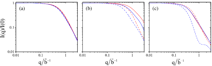
Figure 16: Comparing heteropolymer perturbation theory-predicted and explicit-chain simulated scattering intensities in the $v_{1}^{\pm}$ and $(\epsilon_{\rm p})_{1}^{\pm}$ interaction schemes. Here $I(q)/I(0)$ is computed using $v_{1}^{+}$ and $(\epsilon_{\rm p})_{1}^{+}$ (blue curves) as well as $v_{1}^{-}$ and $(\epsilon_{\rm p})_{1}^{-}$ (red curves), with $v>0$. Perturbation theory-predicted results (dashed curves) are calculated according to Eq. 25 using effective chain length ${\tilde{N}}=43$, effective Kuhn length ${\tilde{b}}=6.46$ Å, $a=1$, and Eqs. 32 and 33 with (a) $v_{0}=0$, $v=0.1$ for $v_{1}^{\pm}$, (b) $v_{0}=0$, $v=0.5$ for $v_{1}^{\pm}$, and (c) $v_{0}=0.1121$—which is the background repulsion corresponding to the $\epsilon_{\rm p}=0$ SAW according to the $I(q)/I(0)$-fitting in Fig. 15a—together with $v=2.5$ for $v_{1}^{+}$ and $v=0.5$ for $v_{1}^{-}$. Explicit-chain simulation results (solid curves) are obtained using Eq. 35, with (a) $\epsilon_{\rm ex}=0$, $v=0.1$ for $(\epsilon_{\rm p})_{1}^{\pm}$, (b) $\epsilon_{\rm ex}=0$, $v=0.5$ for $(\epsilon_{\rm p})_{1}^{\pm}$, and (c) $\epsilon_{\rm ex}=1.0k_{\rm B}T$ (full excluded volume) together with $v=2.5$ for $(\epsilon_{\rm p})_{1}^{+}$ and $v=0.5$ for $(\epsilon_{\rm p})_{1}^{-}$.

Comparisons of theory-predicted and explicit-chain-simulated scattering intensities are provided in Fig. 16 for heteropolymers embodying examples of these $v_{1}^{\pm}$ or $(\epsilon_{\rm p})_{1}^{\pm}$ interactions. Because the baseline (zeroth order term) of our analytical perturbative formula for $I(q)/I(0)$ is that of a Gaussian chain (Eqs. 23–26), we first compare theoretical predictions with simulation results of heteropolymers with no hardcore excluded volume ($\epsilon_{\rm ex}=0$, Figs. 16a,b). In these cases, we find good agreement between theory and simulation when the heteropolymeric interactions are relatively weak ($v=0.1$, Fig. 16a), indicating that the theoretical formulation is effective at a rudimentary level. However, an offset between theoretical and simulated results is seen for stronger heteropolymeric interactions ($v=0.5$, Fig. 16b) although the rank orderings of the $I(q)/I(0)$ entailed by the $v_{1}^{\pm}$ and $(\epsilon_{\rm p})_{1}^{\pm}$ interaction schemes are nonetheless consistent (red curves are higher than blue curves for both the solid and dashed curves in Fig. 16b). This mismatch is probably related to the nonlinear relationship between the $v_{0}$-like and $\epsilon_{\rm p}$-like energy parameters in the theoretical formulation and the explicit-chain model, respectively, as has been observed for homopolymers in Fig. 15b. In this regard, a sizable theory-simulation mismatch is also observed in Fig. 16c, where the simulated $I(q)/I(0)$s are seen to be practically identical for two different SAW heteropolymers ($\epsilon_{\rm ex}=10k_{\rm B}T$) with essentially the same $\langle R^{2}_{\rm g}\rangle^{1/2}\approx 24.1$ Å (solid red and blue curves in Fig. 16c), but the theory-predicted $I(q)/I(0)$s by assuming a linear relationship between the $v_{0}$-like and $\epsilon_{\rm p}$-like energy parameters differ significantly (dashed curves in Fig. 16c). Because the theory-simulation mismatch in Fig. 16c is still quite small for the smaller $v=0.5$ (red curves) and becomes significant only for the larger $v=2.5$ (blue curves), the mismatch here is also likely attributable to a nonlinear relationship between the $v_{0}$-like and $\epsilon_{\rm p}$-like energy parameters as suggested above for the results in Fig. 16b. A resolution of this issue will significantly broaden the utility of the present analytical formulation for heteropolymers and thus deserves to be further investigated in future efforts.

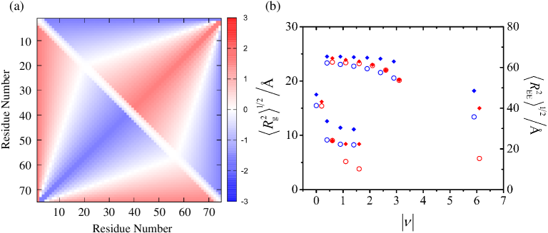
Figure 17: Variations of explicit-chain-simulated root-mean-square radius of gyration and end-to-end distance in the heteropolymeric $(\epsilon_{\rm p})_{1}^{\pm}$ interaction scheme. (a) An example of the energy matrices with matrix elements $[(\epsilon_{\rm p})_{1}^{+}]_{ij}$ (lower triangle) and $[(\epsilon_{\rm p})_{1}^{-}]_{ij}$ (upper triangle) depicted using a color scale (right) for $n=75$ and $v=3.0$. (b) Root-mean-square radius of gyration $\langle R^{2}_{\rm g}\rangle^{1/2}$ (diamonds) and root-mean-square end-to-end distance $\langle R^{2}_{\rm EE}\rangle^{1/2}$ (circles) of chains with full excluded volume ($\epsilon_{\rm ex}=1.0k_{\rm B}T$) for $(\epsilon_{\rm p})_{1}^{+}$, $v=|v|>0$ (blue) and $(\epsilon_{\rm p})_{1}^{-}$, $v=|v|>0$, which is equivalent to $(\epsilon_{\rm p})_{1}^{+}$, $v=-|v|<0$ (red) are plotted slightly offset to the left and to the right, respectively, of $|v|=0.5,1.0,1.5,2.0,2.5,3.0$, and $6.0$. For $|v|=0.1,0.5,1.0$, and $1.5$, corresponding $\langle R^{2}_{\rm g}\rangle^{1/2}$ and $\langle R^{2}_{\rm EE}\rangle^{1/2}$ for $\epsilon_{\rm ex}=0$ (i.e., with Gaussian-chain baseline)—which are always smaller than their counterparts for $\epsilon_{\rm ex}=1.0k_{\rm B}T$—are also included for comparison.

An immediately useful application of the present analytical formulation is to identify explicit-chain models with theory-inspired heteropolymeric interactions that exhibit significant decoupling of $\langle R_{\bf g}^{2}\rangle$ and $\langle R_{\bf EE}^{2}\rangle$. Fig. 17 provides the $\langle R_{\bf g}^{2}\rangle^{1/2}$ and $\langle R_{\bf EE}^{2}\rangle^{1/2}$ values (Fig. 17b) of examples of heteropolymers embodying the $(\epsilon_{\rm p})^{\pm}_{1}$ interaction scheme (Eq. 35) illustrated by the heat maps in Fig. 17a. Consistent with the theoretical prediction in Eq. 34, Fig. 17b shows that for a given $|v|$, the $\langle R^{2}_{\rm g}\rangle^{1/2}$ (diamonds) of the $v>0$ heteropolymer (blue) is always larger than that of the $v<0$ heteropolymer (red). Moreover, the theoretical prediction that a pair of such $(\epsilon_{\rm p})^{\pm}_{1}$-heteropolymers with $\pm|v|$ have equal $\langle R_{\bf EE}^{2}\rangle^{1/2}$ values (blue and red circles) is also realized approximately by those explicit-chain models in Fig. 17b with small to moderate $|v|$ values—i.e., $|v|\leq 3.0$ for SAW ($\epsilon_{\rm ex}=1.0k_{\rm B}T$) heteropolymers and $|v|\leq 0.5$ for $\epsilon_{\rm ex}=0$ heteropolymers without hardcore excluded volume—but not for models with higher $|v|$ values probably because perturbation theory is less accurate for larger $|v|$. As anticipated by theory (Eq. 34), some of the $(\epsilon_{\rm p})^{\pm}_{1}$-heteropolymers have significantly different $\langle R_{\bf g}^{2}\rangle^{1/2}$ values despite having essentially the same $\langle R_{\bf EE}^{2}\rangle^{1/2}$. Examples of such $\langle R^{2}_{\rm g}\rangle$–$\langle R^{2}_{\rm EE}\rangle$ decoupling include the two $|v|=3.0$ SAW $(\epsilon_{\rm p})^{+}_{1}$-heterpolymers with $\langle R^{2}_{\rm EE}\rangle^{1/2}\approx 54$ Å for which $(\langle R^{2}_{\rm g}\rangle/\langle R^{2}_{\rm EE}\rangle)^{1/2}=23.6$Å$/54.8$Å $=0.43$ ($\langle R^{2}_{\rm g}\rangle/\langle R^{2}_{\rm EE}\rangle=0.19$) for $v=+3.0$ (blue symbols) but $(\langle R^{2}_{\rm g}\rangle/\langle R^{2}_{\rm EE}\rangle)^{1/2}=20.2/53.7=0.38$ ($\langle R^{2}_{\rm g}\rangle/\langle R^{2}_{\rm EE}\rangle=0.14$) for $v=-3.0$ (red symbols), and the two $|v|=0.5$ $\epsilon_{\rm ex}=0$, $(\epsilon_{\rm p})^{\pm}_{1}$-heteropolymers with $\langle R^{2}_{\rm EE}\rangle^{1/2}\approx 24$ Å for which $(\langle R^{2}_{\rm g}\rangle/\langle R^{2}_{\rm EE}\rangle)^{1/2}=12.6/24.4=0.52$ ($\langle R^{2}_{\rm g}\rangle/\langle R^{2}_{\rm EE}\rangle=0.26$) for $v=+0.5$ (blue symbols) but $(\langle R^{2}_{\rm g}\rangle/\langle R^{2}_{\rm EE}\rangle)^{1/2}=9.0/24.1=0.37$ ($\langle R^{2}_{\rm g}\rangle/\langle R^{2}_{\rm EE}\rangle=0.14$) for $v=-0.5$ (red symbols).

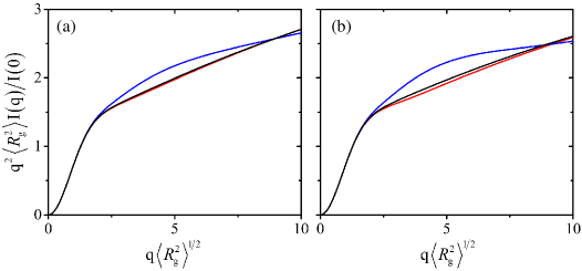
Figure 18: Comparing MFFs of homogeneous and energy-matrix-specified heterogeneous explicit-chain ensembles with full excluded volume ($\epsilon_{\rm ex}=1.0k_{\rm B}T$) and essentially the same $\langle R^{2}_{\rm g}\rangle$. (a) MFFs (dimensionless Kratky plots) of heteropolymer ensembles governed by the $(\epsilon_{\rm p})_{1}^{+}$, $v=2.5$ interactions (blue) and the $(\epsilon_{\rm p})_{1}^{-}$, $v=0.5$ interactions (red), with $\langle R^{2}_{\rm g}\rangle^{1/2}=24.1$ and $24.2$ Å, respectively, are compared with that of the homogeneous $\epsilon_{\rm p}=-0.1$ ensemble with $\langle R^{2}_{\rm g}\rangle^{1/2}=24.2$ Å (black). (b) MFFs of heteropolymer ensembles governed by the $(\epsilon_{\rm p})_{1}^{+}$, $v=3.0$ interactions (blue) and the $(\epsilon_{\rm p})_{1}^{-}$, $v=1.5$ interactions (red), both with $\langle R^{2}_{\rm g}\rangle^{1/2}=23.6$ Å, are compared with that of the homogeneous $\epsilon_{\rm p}=-0.4$ ensemble with $\langle R^{2}_{\rm g}\rangle^{1/2}=23.7$ Å (black).

Scenarios exist within the $(\epsilon_{\rm p})^{\pm}_{1}$ heteropolymeric interaction scheme in Eq. 35 that different heteropolymers sharing essentially the same $\langle R^{2}_{\rm g}\rangle^{1/2}$ can exhibit significantly different SAXS signatures. Two examples are shown in Fig. 18. In both examples, the MFF of the $(\epsilon_{\rm p})^{\pm}_{1}$-heteropolymer with the smaller $|v|$ (red curve) is practically indistinguishable from that of a homopolymer (black curve), which, however, is significantly different from the MFF of the $(\epsilon_{\rm p})^{\pm}_{1}$-heteropolymer with the larger $|v|$ (blue curve). These results reinforce the above observation (Figs. 6, 7, 9, 10, and 13) that SAXS MFFs can sometimes but cannot always distinguish between heterogeneous and homogeneous conformational ensembles.

We now turn to another class of heteropolymeric interactions which is predicted by our perturbation theory to yield pairs of heteropolymers that have the same $\langle R_{\bf g}^{2}\rangle$ but different $\langle R_{\bf EE}^{2}\rangle$s (in contrast to the above $(\epsilon_{\rm p})^{\pm}_{1}$ scheme for heteropolymers with the same $\langle R_{\bf EE}^{2}\rangle$ but different $\langle R_{\bf g}^{2}\rangle$s). For this purpose, we make use of the change in integration variable in Eq. 31 to rewrite the $O(v_{ij})$ term for $\langle R^{2}_{\rm g}\rangle$ in Eq. 17 as

$$-\frac{1}{N^{2}}\int_{a}^{N}d\Delta\tau_{ij}\frac{1}{\sqrt{\Delta\tau_{ij}}}\int_{0}^{N-\Delta\tau_{ij}}d\tau_{i}\;v(\tau_{i},\Delta\tau_{ij}){\cal Z}(N,\tau_{i},\Delta\tau_{ij})\;,$$ (36)

where

$${\cal Z}(N,\tau_{i},\Delta\tau_{ij})\equiv\tau_{i}^{2}-(N-\Delta\tau_{ij})\tau_{i}+\frac{\Delta\tau_{ij}}{12}\Bigl{(}3\Delta\tau_{ij}-4N\Bigr{)}=(\tau_{i}-\lambda)(\tau_{i}-\lambda^{\prime})\;,$$ (37)

with $\lambda=[N-\Delta\tau_{ij}+\Lambda(\Delta\tau_{ij})]/2>0$ and $\lambda^{\prime}=[N-\Delta\tau_{ij}-\Lambda(\Delta\tau_{ij})]/2\leq 0$, wherein $\Lambda(\Delta\tau_{ij})\equiv\sqrt{N(3N-2\Delta\tau_{ij})/3}$. Within the integration range in Eq. 36, the function ${\cal Z}(N,\tau_{i},\Delta\tau_{ij})<0$. For a given $\Delta\tau_{ij}$ and for $\tau_{i}$ values within the range $[0,N-\Delta\tau_{ij}]$, the function takes its maximum (least negative) value of ${\cal Z}_{\rm max}\equiv\lambda\lambda^{\prime}=\Delta\tau_{ij}(3\Delta\tau_{ij}-4N)/12$ at $\tau_{i}=0$ and $N-\Delta\tau_{ij}$, and its minimum (most negative) value of $-\Lambda(\Delta\tau_{ij})^{2}/4=N(2\Delta\tau_{ij}-3N)/12$ at $\tau_{i}=(N-\Delta\tau_{ij})/2$. These considerations indicate that the following two model heteropolymer interaction schemes, $v(\tau_{i},\Delta\tau_{ij})=v^{+}_{2}$ and $v^{-}_{2}$, defined by

$$v^{\pm}_{2}(\tau_{i},\Delta\tau_{ij})=v_{0}+u^{\pm}(\tau_{i},\Delta\tau_{ij})\frac{{\cal Z}_{\rm max}}{{\cal Z}(N,\tau_{i},\Delta\tau_{ij})}\;,$$ (38)

where $u^{\pm}(\tau_{i},\Delta\tau_{ij})$ is from Eq. 33, will give the same $\langle R^{2}_{\rm g}\rangle$ in Eq. (17). This property of $v_{2}^{\pm}$ is readily verified by using either of them for $v(\tau_{,}\Delta\tau_{ij})$ in Eq. 36 to yield the same $O(v_{ij})$ term for $\langle R^{2}_{\rm g}\rangle$. As is the case for $v_{1}^{\pm}$, $v_{2}^{\pm}=v_{0}\mp v$ at $\tau_{i}=0$ and $\tau_{i}=N-\Delta\tau_{ij}$. The model interactions $v_{2}^{\pm}$ are of interest because according to Eq. 9 they should lead to two different $\langle R^{2}_{\rm EE}\rangle$ values, denoted here as $\langle R^{2}_{\rm EE}\rangle_{v^{+}_{2}}$ and $\langle R^{2}_{\rm EE}\rangle_{v^{-}_{2}}$. Their $O(v_{ij})$ difference is given by

$$\langle R^{2}_{\rm EE}\rangle_{v^{+}_{2}}-\langle R^{2}_{\rm EE}\rangle_{v^{-}_{2}} = 2\int_{a}^{N}dx\;\sqrt{x}(3x-4N)\int_{0}^{N-x}dy\;\frac{u^{+}(y,x)}{{\cal Z}(N,y,x)}$$ (39)

$$= 4v\int_{a}^{N}dx\;\sqrt{x}(4N-3x)\biggl{\{}\frac{1}{\Lambda(x)}\ln\biggl{[}\frac{\Lambda(x)+N-x}{\Lambda(x)-N+x}\biggr{]}$$

$$\quad\quad\quad\quad\quad\quad\quad\quad\quad\quad-\frac{2}{N-x}\ln\biggl{[}\frac{N(3N-2x)}{x(4N-3x)}\biggr{]}\biggr{\}}$$

$$\approx -1.67(vN^{3/2})\quad(a\rightarrow 0)\;,$$

where we have used the variables $x$ and $y$ for $\Delta\tau_{ij}$ and $\tau_{i}$, respectively. In the same manner in which we arrived at Eq. 35, a discrete version of $v_{2}^{\pm}$ may be given by pairwise interaction energies

$$[(\epsilon_{\rm p})_{2}^{\pm}]_{ij}\equiv\frac{\Delta_{ij}[3\Delta_{ij}-4(n-1)]/12}{{\cal Z}(n-1,i-1,\Delta_{ij})}[(\epsilon_{\rm p})_{1}^{\pm}]_{ij}\;,$$ (40)

where the function ${\cal Z}$ is now evaluated for $N=n-1$ at discrete values of $i=1,2,\dots,n-\Delta_{ij}$ and $[(\epsilon_{\rm p})_{1}^{\pm}]_{ij}$ is defined by Eq. 35 above. An example of the $(\epsilon_{\rm p})_{2}^{\pm}$ interaction scheme in Eq. 40 is provided by the heat maps in Fig. 19a.

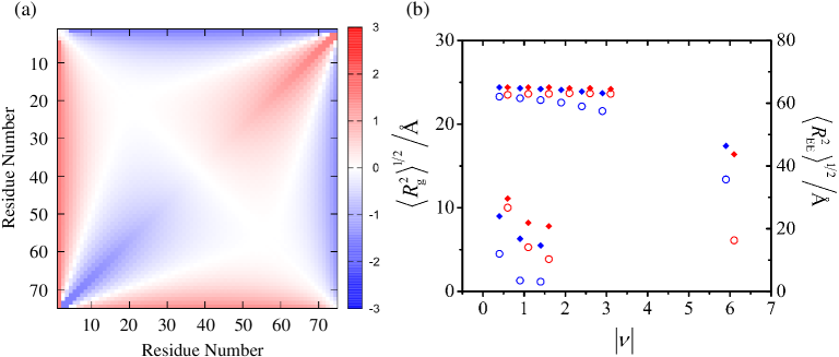
Figure 19: Variations of explicit-chain-simulated $\langle R^{2}_{\rm g}\rangle^{1/2}$ and $\langle R^{2}_{\rm EE}\rangle^{1/2}$ in the heteropolymeric $(\epsilon_{\rm p})_{2}^{\pm}$ interaction scheme in Eq. 40. (a) Similar to Fig. 17a for $(\epsilon_{\rm p})_{1}^{\pm}$, here $[(\epsilon_{\rm p})_{2}^{+}]_{ij}$ (lower triangle) and $[(\epsilon_{\rm p})_{2}^{-}]_{ij}$ (upper triangle) are shown for $n=75$ and $v=3.0$. (b) Using the same notation as that in Fig. 17b, $\langle R^{2}_{\rm g}\rangle^{1/2}$ (diamonds) and $\langle R^{2}_{\rm EE}\rangle^{1/2}$ (circles) for $(\epsilon_{\rm p})_{2}^{+}$, $v=|v|>0$ (blue) and $(\epsilon_{\rm p})_{2}^{-}$, $v=|v|>0$ (red) are shown for full excluded volume ($\epsilon_{\rm ex}=1.0k_{\rm B}T$) at $|v|=0.5,1.0,1.5,2.0,2.5,3.0$, and $6.0$, and also for the $\epsilon_{\rm ex}=0$ (Gaussian-chain baseline) case at $|v|=0.5,1.0$, and $1.5$.

The SAW examples ($\epsilon_{\rm ex}=10k_{\rm B}T$) in Fig. 19b of explicit-chain simulated $\langle R^{2}_{\rm g}\rangle^{1/2}$ and $\langle R^{2}_{\rm EE}\rangle^{1/2}$ values of heteropolymers embodying the $(\epsilon_{\rm p})_{2}^{\pm}$ interaction scheme are largely in line with the theoretical prediction that a pair of $(\epsilon_{\rm p})_{2}^{\pm}$-heteropolymers with the same $|v|$ should have the same $\langle R^{2}_{\rm g}\rangle^{1/2}$ (diamonds)—which is essentially the case for $|v|\leq 3.0$ and holds approximately for $|v|=6.0$—but increasingly different $\langle R^{2}_{\rm EE}\rangle^{1/2}$s (circles) with increasing $|v|$. (We note, however, that while the sign of the difference in $\langle R^{2}_{\rm EE}\rangle^{1/2}$ for the $v>0$ and $v<0$ $(\epsilon_{\rm p})_{2}^{+}$-heterpolymers with the same $|v|$ is consistent with Eq. 39 for $|v|\leq 3.0$, the sign is opposite for $|v|=6.0$). Therefore, although the theory does not appear to work well for the $\epsilon_{\rm ex}=0$ chains in Fig. 19b (data points at bottom left), the simulated data on SAW $(\epsilon_{\rm p})_{2}^{+}$-heteropolymers provide ample examples of $\langle R^{2}_{\rm g}\rangle$–$\langle R^{2}_{\rm EE}\rangle$ decoupling, including the case of $|v|=3.0$ in which $(\langle R^{2}_{\rm g}\rangle/\langle R^{2}_{\rm EE}\rangle)^{1/2}=23.7$Å$/57.5$Å $=0.41$ ($\langle R^{2}_{\rm g}\rangle/\langle R^{2}_{\rm EE}\rangle=0.17$) for $v=+3.0$ (blue symbols) but $(\langle R^{2}_{\rm g}\rangle/\langle R^{2}_{\rm EE}\rangle)^{1/2}=24.2/63.0=0.38$ ($\langle R^{2}_{\rm g}\rangle/\langle R^{2}_{\rm EE}\rangle=0.15$) for $v=-3.0$ (red symbols) though the $\langle R^{2}_{\rm EE}\rangle^{1/2}\sim 24$ Å of these two heteropolymers are quite similar, and the case of $|v|=6.0$ in which $(\langle R^{2}_{\rm g}\rangle/\langle R^{2}_{\rm EE}\rangle)^{1/2}=17.4/31.5=0.55$ ($\langle R^{2}_{\rm g}\rangle/\langle R^{2}_{\rm EE}\rangle=0.31$) for $v=+6.0$ (blue symbols) but $(\langle R^{2}_{\rm g}\rangle/\langle R^{2}_{\rm EE}\rangle)^{1/2}=16.4/16.3=1.0$ for $v=-6.0$ (red symbols) though the $\langle R^{2}_{\rm EE}\rangle^{1/2}$ values of $\sim 17$ Å for this pair of $|v|=6.0$ $(\epsilon_{\rm p})_{2}^{\pm}$-heteropolymers are also quite similar.

Figure 20: Variations of explicit-chain-simulated $\langle R^{2}_{\rm g}\rangle^{1/2}$ and $\langle R^{2}_{\rm EE}\rangle^{1/2}$ in the heteropolymeric $(\epsilon_{\rm p})_{3}^{\pm}$ interaction scheme (Eq. 44). (a) Similar to Figs. 17a and 18a, here $[(\epsilon_{\rm p})_{3}^{+}]_{ij}$ (upper triangle) and $[(\epsilon_{\rm p})_{2}^{-}]_{ij}$ (lower triangle) are shown for $n=75$ and $v=100.0$. In this case, although $\min\{[(\epsilon_{\rm p})_{3}^{+}]_{ij}\}=-100$ and $\max\{[(\epsilon_{\rm p})_{3}^{-}]_{ij}\}=+100$, a graded color scale for $[-3,+3]$ (with all $[(\epsilon_{\rm p})_{3}^{+}]_{ij}\leq-3$ and all $[(\epsilon_{\rm p})_{3}^{-}]_{ij}\geq+3$ depicted, respectively, by the same deepest blue and red) is used to visualize variation in pairwise energy because $|[(\epsilon_{\rm p})_{3}^{\pm}]_{ij}|$ is relatively small for most $i,j$. (b) Using the same notation as that in Figs. 17b and 18b, $\langle R^{2}_{\rm g}\rangle^{1/2}$ (diamonds) and $\langle R^{2}_{\rm EE}\rangle^{1/2}$ (circles) for $(\epsilon_{\rm p})_{3}^{+}$, $v=|v|>0$ (red) and $(\epsilon_{\rm p})_{3}^{-}$, $v=|v|>0$, which is equivalent to $(\epsilon_{\rm p})_{3}^{+}$, $v=-|v|<0$ (blue), are shown for full excluded volume ($\epsilon_{\rm ex}=1.0k_{\rm B}T$) at $|v|=0.5,1.0,1.5,2.0,2.5,3.0$, $6.0$, $10.0$, $12.0$, $14.0$, $16.0$, $18.0$, $20.0$, $25.0$, $50.0$, and $100.0$. Unlike Figs. 17b and 18b, no data for the Gaussian-chain, $\epsilon_{\rm ex}=0$ baseline case is shown.

Another class of heterogeneous interactions predicted by our perturbation theory to keep $\langle R^{2}_{\rm g}\rangle$ unchanged while changing $\langle R^{2}_{\rm EE}\rangle$ is given by $v_{ij}=v(\tau_{i},\tau_{j})=v(\Delta\tau_{ij})$, which is a function of $\Delta\tau_{ij}$ alone to be defined below. In other words, in this interaction scheme, all intrachain contacts of the same order have the same energy but intrachain contacts with different contact orders have different energies. Consider

$$v_{3}^{\pm}(\Delta\tau_{ij})\equiv v_{0}\mp{\tilde{v}}_{3}\frac{\sqrt{\Delta\tau_{ij}}}{(N-\Delta\tau_{ij})(2N^{2}-\Delta\tau_{ij}^{2})}\Bigl{(}2\Delta\tau_{ij}-N-a\Bigr{)}\;$$ (41)

where ${\tilde{v}}_{3}$ is an adjustable energy scale. Under $v_{3}^{\pm}$ and for a given $|{\tilde{v}}_{3}|$, $\langle R^{2}_{\rm g}\rangle$ is the same irrespective of whether the minus or plus sign is taken for the $\mp$ sign in Eq. 41 because the $O(v_{ij})$ term for $\langle R^{2}_{\rm g}\rangle$ (Eq. 36) with $v_{3}^{\pm}$ is equal to

$$-\frac{1}{N^{2}}\int_{a}^{N}d\Delta\tau_{ij}\frac{v_{3}^{\pm}(\Delta\tau_{ij})}{\sqrt{\Delta\tau_{ij}}}\int_{0}^{N-\Delta\tau_{ij}}d\tau_{i}\;{\cal Z}(N,\tau_{i},\Delta\tau_{ij})=0\;.$$ (42)

In contrast, the sign choice would affect $\langle R_{\rm EE}^{2}\rangle$, as can be readily verifed that the $O(v_{ij})$ difference in $\langle R_{\rm EE}^{2}\rangle$ calculated using $v_{3}^{+}$ verus that calculated using $v_{3}^{-}$ is given by

$$\langle R^{2}_{\rm EE}\rangle_{v^{+}_{3}}-\langle R^{2}_{\rm EE}\rangle_{v^{-}_{3}} = \frac{{\tilde{v}}_{3}}{\sqrt{2}}\biggl{\{}[(2\sqrt{2}+1)+a/N]\ln\biggl{(}\frac{\sqrt{2}+1}{\sqrt{2}+a/N}\biggr{)}$$ (43)

$$\quad\quad\quad\quad\quad\quad+[(2\sqrt{2}-1)-a/N]\ln\biggl{(}\frac{\sqrt{2}-1}{\sqrt{2}-a/N}\biggr{)}\biggr{\}}\;,$$

which equals $-0.140{\tilde{v}}_{3}$ in the $a/N\rightarrow 0$ limit. We obtain a discretized version of this interaction scheme by setting $N\rightarrow n=N+1$ in Eq.41 to arrive at

$$[(\epsilon_{\rm p})_{3}^{\pm}]_{ij}=\mp v\frac{\sqrt{\Delta_{ij}}(2\Delta_{ij}-n-a)}{(n-\Delta_{ij})(2n^{2}-\Delta_{ij}^{2})}\left[\frac{n^{2}+2n-1}{\sqrt{n-1}\;(n-2-a)}\right]\;$$ (44)

and by choosing $a=3$. Accordingly, the above interaction scheme $(\epsilon_{\rm p})_{3}^{\pm}$ in Eq. 44 is defined for $\Delta_{ij}=a=3,4,\dots,n-1$, where the expression inside the square bracket is a normalization factor such that $|v|$ is the magnitude of the interaction for the largest contact order $\Delta_{ij}=n-1$ (Fig. 20a).

The SAW examples ($\epsilon_{\rm ex}=10k_{\rm B}T$) in Fig. 20b of explicit-chain simulated $\langle R^{2}_{\rm g}\rangle^{1/2}$ and $\langle R^{2}_{\rm EE}\rangle^{1/2}$ values of heteropolymers embodying the $(\epsilon_{\rm p})_{3}^{\pm}$ interaction scheme show little variation for $|v|\lesssim 12$. For $|v|\gtrsim 14$, $\langle R^{2}_{\rm EE}\rangle^{1/2}$ of $(\epsilon_{\rm p})_{3}^{+}$-heteropolymers with $v>0$ (blue circles) decreases steeply with increasing $|v|$. Although the corresponding $\langle R^{2}_{\rm g}\rangle^{1/2}$ (blue diamonds) also decreases concomitantly in a trend that differs from the perturbation theory prediction of unchanged $\langle R^{2}_{\rm g}\rangle^{1/2}$, the rate of decrease of $\langle R^{2}_{\rm g}\rangle^{1/2}$ with increasing $|v|$ is more gradual than that of $\langle R^{2}_{\rm EE}\rangle^{1/2}$ as one might intuitively anticipate from an approximate theory. In this regard, Fig. 20b provides a few examples of dramatic $\langle R^{2}_{\rm g}\rangle$–$\langle R^{2}_{\rm EE}\rangle$ decoupling, including a pair of $|v|=20.0$ $(\epsilon_{\rm p})_{3}^{+}$-heteropolymers for which $(\langle R^{2}_{\rm g}\rangle/\langle R^{2}_{\rm EE}\rangle)^{1/2}=20.9$Å$/41.4$Å $=0.50$ ($\langle R^{2}_{\rm g}\rangle/\langle R^{2}_{\rm EE}\rangle=0.25$) for $v=+20.0$ (blue symbols) but $(\langle R^{2}_{\rm g}\rangle/\langle R^{2}_{\rm EE}\rangle)^{1/2}=24.3/62.3=0.39$ ($\langle R^{2}_{\rm g}\rangle/\langle R^{2}_{\rm EE}\rangle=0.15$) for $v=-20.0$ (red symbols), and a pair of $|v|=50.0$ $(\epsilon_{\rm p})_{3}^{+}$-heteropolymers for which $(\langle R^{2}_{\rm g}\rangle/\langle R^{2}_{\rm EE}\rangle)^{1/2}=17.6/3.7=4.8$ ($\langle R^{2}_{\rm g}\rangle/\langle R^{2}_{\rm EE}\rangle=22.6$) for $v=+50.0$ (blue symbols), which is much higher than that of any homopolymer ensemble shown in the inset of Fig. 3a, but $(\langle R^{2}_{\rm g}\rangle/\langle R^{2}_{\rm EE}\rangle)^{1/2}=24.3/62.2=0.39$ ($\langle R^{2}_{\rm g}\rangle/\langle R^{2}_{\rm EE}\rangle=0.15$) for $v=-50.0$ (red symbols).

DISCUSSION

The logic of inferring conformational ensembles from MFFs. Considered in aggregate, the results presented above show that having a homopolymer-like MFF is insufficient to guarantee an underlying homogeneous conformational distribution, although having a non-homopolymer-like MFF is a good indication of a heterogeneous ensemble. Proteins are heteropolymers. Therefore, physically, it is most intuitive to expect disordered conformational ensembles of proteins to be heterogeneous even if, somehow, their MFFs turn out to be homopolymer-like. Indeed, recent explicit-chain simulations using a coarse-grained potential with a simple sidechain representation for real IDPs have shown that such behavior is possible—as seen also in the mathematically constructed examples we showcase above—in that conformational ensembles with asphericity and another shape parameter significantly different from those of homopolymer can nonetheless exhibit scattering intensities similar to those of homopolymersDT2019 (though the simulation-experiment agreement is apparently closer for $I(q)/I(0)$–vs–$q$ plots than for $q^{2}I(q)/I(0)$–vs–$q$ (Kratky) plots reported, respectively, in Fig. 2 and Fig. S1 of this reference). In view of this basic consideration, it would not be prudent to invoke Occam’s razor and simply infer a homogeneous ensemble as the most parsimonious interpretation of the SAXS data when confronted with a homopolymer-like MFF for a disordered protein ensemble when complementary experimental techniques are available to gain further insight into the structural properties of the ensemble.lemke2017 ; raleighPNAS2019 ; raleighBiochem2020 In this regard, a recent statistical survey of ensembles of model heteropolymers (which are, by construction, heterogeneous ensembles) with intrachain hydrohobic-polar (HP)-like interactions exhibiting conformational averages of $R_{\rm g}$ and $R_{\rm EE}$ coupled approximately in a manner similar to the $\langle R^{2}_{\rm g}\rangle$–$\langle R^{2}_{\rm EE}\rangle$ coupling in homopolymers as well as having MFFs not so dissimilar to those for homopolymerstobinPNAS2019 provides additional illustrations for our thesis that MFFs alone are insufficient to clearly distinguish between heterogeneous and homogeneous ensembles. At the same time, it should be emphasized that HP-like interactions cover only a subset of intraprotein interactions. In fact, HP-like interactions alone cannot produce the high degree of folding cooperativity (see below) observed experimentally for small, single-domain proteins.chanetal2004 ; Chan2000 As discussed above, using our analytical theory-inspired heteropolymeric interactions—although that still neglect a lot of other modes of intraprotein interactions, we are able to provide ample examples of $\langle R^{2}_{\rm g}\rangle$–$\langle R^{2}_{\rm EE}\rangle$ decoupling in heterogeneous ensembles. From a biological/evolutionary perspective, one should expect that any feature of conformational heterogeneity of disordered protein ensembles—including $\langle R^{2}_{\rm g}\rangle$–$\langle R^{2}_{\rm EE}\rangle$ decoupling—can be potentially exploited for biological function. As researchers, it would be unwise to self-impose a priori boundaries to box in our imagination of conformational possibilities.

Conformational heterogeneity and physical pictures of folding cooperativity. SAXS was instrumental in revealing an important aspect of two-state-like folding cooperativity of small, single-domain proteins by observing directly, in a time-resolved manner, that the unfolded state of Protein L is consisted of relatively open conformations (large $\langle R^{2}_{\rm g}\rangle$) even under strongly folding conditions.Plaxco1999 This finding was remarkable from a theoretical perspective because common protein chain models at the time predicted a substantial decrease of $\langle R^{2}_{\rm g}\rangle$ of the unfolded conformational ensemble when its solvent environment is changed from strongly unfolding (as in high denaturant) to strongly folding (as in low or no denaturant). Two-state folding/unfolding cooperativity has since been found to be intimately relatedchanetal2004 to contact-order-dependent folding ratesPlaxco1998 and linear chevron plots, as protein chain models with reduced cooperativity—hallmarked by an appreciable decrease in unfolded-state $\langle R^{2}_{\rm g}\rangle$ with increasingly strong folding conditions—failed to reproduce these experimental features.chanetal2004 ; ChanNat1998 ; kaya2003d This early success in applying folding cooperativity—with unfolded states with large conformational dimensions minimally affected by folding conditions—as a basic, unifying rationalization of the defining experimentally observed features in the folding of small, single-domain proteins has led some researchers to an extreme view of two-state folding cooperativity known as the topomer search model of protein folding.topomer2003 In this view, the unfolded state of a globular protein is envisioned as behaving like—and thus modeled by—homopolymeric Gaussian chains without excluded volume, and folding is stipulated to be achieved by random diffusive searching of a “native topomer” among these conformations.topomer2003 Apparently, the rationale of this perspective is that experimental observations, such as SAXS data, that the authors interpreted as implying a homogeneous ensemble of open unfolded conformations—with excluded volume or not—should take precedence over any theoretical concern as to how the existence of such an ensemble may follow from current understanding of the driving forces for protein folding. In other words, if commonly accepted physical interactions cannot account for what the authors viewed as experimental facts about the homopolymer-like unfolded-state ensemble, the fault is with common theoretical understanding; and, therefore, rather than casting doubt on the topomer search model as physically unrealizable, it is the commonly accepted theoretical understanding of protein folding driving forces that needs to be revised and improved.

A contrasting philosophy, which might be common among theoreticians, is to place more trust on current theoretical notions about protein folding driving forces and accept them as approximately correct. Researchers subscribing to this line of thinking tend to emphasize interpreting experimental data in terms of what is perceived to be physically plausible; thus the accuracies of experiments that appear inconsistent with pre-conceived notions of physical interactions are often questioned. As it stands, explicit-chain heteropolymeric protein models embodying current notions of physical interactions—even when common structurally-specific native-centric models are included—possess less overall folding cooperativity than that of many real, small, single-domain proteins.KayaPRL2003 In particular, these heteropolymer models entail unfolded conformations with decreased average $R_{\rm g}$ with stronger folding conditions.DT2008 While this explicit-chain heteropolymer model-predicted picture was apparently at odds with inferences from SAXS experimentPlaxco1999 and in-depth understanding of calorimetric two-state folding cooperativity,chanetal2004 ; chanetal2011 ; kayaProteins2000 ; mk2006 it was apparently supported by smFRET experiments on Protein L for which decreasing $\langle R^{2}_{\rm g}\rangle$ with decreasing denaturant was inferred using an interpretation of smFRET data (which measured $\langle R_{\rm EE}\rangle$ but not $\langle R^{2}_{\rm g}\rangle$ directly) that assumed homopolymeric $\langle R^{2}_{\rm g}\rangle$–$\langle R^{2}_{\rm EE}\rangle$ coupling.haran2006

In our estimation, an awareness of this historical background is contextually useful for appreciating the different investigative logic and contrasting conceptual emphases in the controversy surrounding the apparent mismatch of smFRET- versus SAXS-determined conformational dimensions of protein disordered states.tobinkevinJMB2012 ; tobinkevinPNAS2015 ; haran2012 ; dt2009 ; Songetal2015

A “near-Levinthal” scenario of cooperative protein folding. A synthesis of the useful insights from the two above-described approaches needs to consider the following. First, as a proposed physical mechanism, the topomer search model—which assumes that an unfolded protein state is a noninteracting homogeneous ensemble—is untenable because this hypothetical mechanism entails a kinetically impossible Levinthal search when excluded volume of the chains are (as it should be) taken into account.WallinChan2005 Nonetheless, the discourse inspired by the model’s emphasis on the high degrees of folding cooperativity is valuable because a comprehensive theoretical understanding of physical interactions in protein folding should be able to account for this experimental property. Second, explicit-chain heteropolymer models of protein disordered states are valuable in underscoring the sequence-dependent heterogeneous nature of these conformational ensemble. However, it is important to recognize the limitations of current understanding of the solvent-mediated protein interactions.DavidShaw2 ; cosb15 A case in point is that even native-centric models with only pairwise interactions cannot reproduce the high degree of folding cooperativity of Protein L,TaoPCCP and that yet-undiscovered non-parwise-additive many-body effects, such as local-nonlocal coupling, are possibly implicated in protein folding cooperativity.chanetal2011 ; kaya2003d

A conceptual picture of cooperative folding that takes all these considerations into account is referred to as a “near-Levinthal” scenario.kaya2003c This picture of folding expects, because of basic physics, that the unfolded state is a heterogeneous ensemble and that conformational search during folding must experience a certain bias toward the native structure because in the absence of any bias, folding would be kinetically impossible (Levinthal’s paradox). At the same time, it is stipulated that the bias, though not nonexistent, is relatively weak because if the bias is strong—implying that intrachain interactions are strongly favorable—the unfolded state under folding conditions would be a relatively compact conformational ensemble rather than the open conformational ensemble observed experimentally. Finally, in this “near-Levinthal” picture of folding, the folded state is envisioned to be thermodynamically stabilized by certain strongly favorable interactions, perhaps via many-body mechanisms such as the proposed local-nonlocal coupling effects, that are operative only after the protein has crossed to the folded side of the transition-state free energy barrier but not in the unfolded state.chanetal2011 Recent advances in smFRET data interpretation and SAXS experiments lend credence to this picture: First, it is now recognized that a larger $\langle R^{2}_{\rm g}\rangle^{1/2}$ can be consistent with smFRET data on protein unfolded state because of possible $\langle R^{2}_{\rm g}\rangle$–$\langle R^{2}_{\rm EE}\rangle$ decoupling in heterogeneous ensembles.Songetal2017 Second, more accurate SAXS measurements indicate a small contraction of unfolded-state ensembles when denaturant concentration is reduced,tobinSci2017 indicating that denaturant-dependent favorable intrachain interactions are present in the unfolded state. Given that these interactions should be sequence-dependent, this SAXS observation is likely indicative of a heterogeneous unfolded-state ensemble.

Water as solvent for proteins. The SAXS-observed phenomenon that the unfolded states of many globular proteins remain quite open even under strongly folding conditions (as in water), which is a hallmark of protein folding cooperativity, has recently been cast in terms of “water is a good solvent for the unfolded states of many proteins”.TobinJMBrev2020 While this narrative may serve to highlight the different solvation properties of homopolymeric versus evolved heteropolymeric disordered protein states and the rhetoric may focus attention on the important ramifications of folding/unfolding cooperativity as emphasized in the above discussion (and in references thereof) as well as by the authors of this review,TobinJMBrev2020 application of “solubility” to a state, i.e., a subpopulation, of a molecular species rather than the total population of the molecular species as a whole may not enhance conceptual clarity. In the conventional meaning of the term, solubility of a solute in a solvent refers to the global miscibility of the solvent and the solute, not a subpopulation of the solute. While the unfolded chains of a soluble protein is, by definition, solvated to various degree, only a very small fraction of the chain population is unfolded under the strongly folding conditions of pure water. Now, if one applies the same nomenclatural logic in ref. (141) that water is a good solvent of unfolded states of some proteins to a more mundane system of nonpolar solutes and water, one can arrive at a tautological, and thus uninformative, proposition that water is a good solvent for the solvated state of the nonpolar solute (i.e., the minute solvated fraction of the nonpolar substance) even when the overwhelming population of the substance is not solvated and the substance is practically insoluble. In this regard, describing the role of hydrophobicity in protein folding by the traditional dictum “water is a poor solvent for the unfolded state of globular proteins” is less problematic because, semantically consistent with the “poor solvent” characterization, an overwhelming majority of the chain population is folded (i.e., not “solvated” as unfolded chains) in water. Nonetheless, the “poor solvent” narrative can also be misleading. This is because in this case poor solvation in water applies only to part of the protein molecule (e.g., nonpolar residues) but not every part of the heteropolymeric protein chain. In fact, globular proteins are soluble as individual folded molecules in water. In other words, water is a good—not poor—solvent for the individual protein molecules as a whole. Unqualified usage of the “poor solvent” description may therefore mask important biophysical and functional distinctions among disordered protein states of different compactness,TobinJMBrev2020 differences that are crucial for categorizing noncooperative and various types of cooperative folding.chanetal2004 ; chanetal2011 ; kayaProteins2000 Taking all the above into consideration, it is apparent that invocation of aqueous solubility of subpopulations of a protein’s conformational ensemble risk unnecessary confusion and such narratives are not always conducive to a clear conceptualization of protein folding.

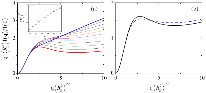
Figure 21: MFFs of composite ensembles. (a) Dimensionless Kratky plots of the $C=0.1,0.2,\dots,0.9$ composite ensembles with $\epsilon_{\rm p}^{(1)}=+2.0$ and $\epsilon_{\rm p}^{(2)}=-2.0$ (Eq. 46) with different overall $\langle R^{2}_{\rm g}\rangle^{1/2}$ values (inset) are plotted using the same color code. Dimensionless Kratky plots for the homogeneous $\epsilon_{\rm p}^{(1)}=+2.0$ ($C=1.0$, dark blue) and the homogeneous $\epsilon_{\rm p}^{(2)}=-2.0$ ($C=0$, red) ensembles are shown by thicker curves. (b) Dimensionless Kratky plot for $C=0.1$ (solid curve) heteropolymeric composite ensemble (overall $\langle R^{2}_{\rm g}\rangle^{1/2}=18.3$ Å) is compared with that for the $\epsilon_{\rm p}=-1.8$ homogeneous ensemble with $\langle R^{2}_{\rm g}\rangle^{1/2}=18.5$ Å (dashed curve). The $I(q)$s of the $C$-dependent heterogeneous ensembles in (a) are also compared using other plotting formats in Fig. S7 of Supporting Information.

Composite ensembles and experimental uncertainties. As emphasized above, in addition to the cases studied so far by us and by others, one expects that there are many other scenarios in which heterogeneous ensembles are not readily distinguishable from homopolymer ensembles by MFFs alone. As a further example, consider a heterogeneous ensemble which is a superposition of two homogeneous ensembles defined by two different $\epsilon_{\rm p}$ values symbolized as $\epsilon_{\rm p}^{(1)}$ and $\epsilon_{\rm p}^{(2)}$. A situation similar to this hypothetical scenario readily arise when there is a mixture of folded and unfolded protein conformations in an overall ensemble,Plaxco1999 ; raleighBiochem2020 or when there is a bimodal-like distribution of conformational properties of an IDP, as has been suggested computationally.tanja2010 Now, let the $\langle R^{2}_{\rm g}\rangle$ of the two component homogeneous ensembles be $\langle R_{\rm g}^{2}\rangle^{(1)}$ and $\langle R_{\rm g}^{2}\rangle^{(2)}$, respectively, and the corresponding be scattering intensities be $I^{(1)}(q)$ and $I^{(2)}(q)$. The $\langle R^{2}_{\rm g}\rangle$ of a composite conformational ensemble with weights of $C$ and $1-C$ for the $\epsilon_{\rm p}^{(1)}$- and $\epsilon_{\rm p}^{(2)}$-ensembles ($0\leq C\leq 1$), respectively, is then given by

$$\langle R_{\rm g}^{2}\rangle=C\langle R_{\rm g}^{2}\rangle^{(1)}+(1-C)\langle R_{\rm g}^{2}\rangle^{(2)}\;,$$ (45)

and the corresponding scattering intensity is given by

$$I(q)=CI^{(1)}(q)+(1-C)I^{(2)}(q)\;,$$ (46)

and $I_{0}=CI^{(1)}(0)+(1-C)I^{(2)}(0)$. The SAXS signatures of such a system are shown in Fig. 21. A comparison is highlighted in Fig. 21b between the MFF of a $C=0.1$ heterogeneous composite ensemble (solid curve) and that of a homopolymer ensemble with the same $\langle R^{2}_{\rm g}\rangle^{1/2}$ (dashed curve). The result indicates that the two theoretical MFFs are distinct and therefore distinguishable in principle, especially in situation where a mixture of conformational species is expected as in the study of protein folding/unfolding.Plaxco1999 ; raleighBiochem2020 At the same time, the similarity between the MFFs also suggests that the heterogeneous and homogeneous ensembles may not be easily discriminated by their MFFs alone without prior knowledge of a complex conformational distribution and in the face of possible experimental uncertainties.DT2008 The theoretical approach we have taken here is agnostic as to experimental accuracy, using a coarse-grained chain model without atomistic details and ignoring any explicit consideration of solvation effects for the purpose of exploring conceptual principles. Nonetheless, it is worth mentioning that some of the fitted homopolymeric MFFs for disordered protein ensembles reported in the literature exhibit significant deviations from experimental data for $q$ values not much larger than those in the shoulder region of the dimensionless Kratky plot (e.g., the [KCl] = 0.15 M data in Fig. 3C of ref. (93) and Fig. S5 in ref. (116)). Other effects, such as those associated with the hydration shell around the protein,skepo2018 may add further uncertainties in matching simulated and experimental MFFs and thus render the inference of conformational ensembles from MFFs more challenging.

CONCLUSIONS

To recapitulate, basic physics stipulates that disordered conformational ensembles of unfolded proteins and IDPs are, in general, heterogeneous because proteins are heteropolymers of amino acid residues. MFFs obtained from SAXS of disordered protein ensembles are valuable because they yield more structural information about conformational ensembles from higher-$q$ parts of $I(q)$, whereas this information is unavailable from small-$q$ Guinier analyses which afford only an overall $\langle R^{2}_{\rm g}\rangle$ (refs. (93; 94; 95; 96)). Nonetheless, structural information from MFFs is still highly averaged. As exemplified by recent simulation of several IDPs,DT2019 the systematic analysis conducted in the present work has shown that the MFF of a heterogeneous ensemble is not always distinct from that of a homogeneous ensemble. In not a few instances, MFFs cannot reliably distinguish between heterogeneous from homogeneous disordered conformational ensembles with the same $\langle R^{2}_{\rm g}\rangle$. Clearly, then, the conformational ensemble to MFF correspondence is practically a many-to-one mapping. Not only that, this mapping is likely not smooth—meaning that while small changes in conformational ensemble lead to only small changes in MFF, small changes or experimentally indiscernible minute changes in MFF can map to structurally drastically different conformational ensembles. We have now demonstrated, mathematically, the many-to-one and non-smooth features of the (ensemble $\rightarrow$ MFF) mapping by identifying various heterogeneous ensembles with MFFs very similar to those of homopogeneous ensembles. These heterogeneous ensembles with homopolymer-like MFFs include some of the conformationally highly restricted $(R_{\rm g},R_{\rm EE})$ subensemblesSongetal2015 ; Songetal2017 ; DICE which may be viewed as members of a conformational-space basis set (Figs. 7–9), computationally selected reweighted ensembles with exceptionally similar MFFs but significanty different distributions of $R_{\rm g}^{2}$, $R^{2}_{\rm EE}$, and asphericity (Fig. 13) as well as intuitively plausible ensembles with narrower-than-SAW distributions of $R^{2}_{\rm g}$ and compact-open composite ensembles (Figs. 10 and 21). These counterexamples to any preconception or tacit assumption of a one-to-one ensemble-MFF mapping highlight the intrinsic logical uncertainty when one attempts to infer a conformational ensemble from a given MFF.

In view of the limited current knowledge about the effects of the sequence-dependenttanja08 ; PatriciaPNAS2020 physical interactions on conformational dimensions and other structural properties of IDPs and unfolded states of cooperatively-folding globular proteins,chanetal2011 ; DavidShaw2 ; cosb15 it is not possible to determine a priori which ensemble/structural properties of disordered proteins are physically encodable by amino acid sequences and which properties are not. As our ability to imagine what is physically possible for disordered protein conformations is so limited because of this lack of knowledge, aside from obvious cases, one cannot preclude many of the heterogeous ensembles with homopolymer-like MFFs as physically unrealizable. Therefore, the logico-mathematical uncertainty that we have established regarding any inference of conformational ensemble that is based solely on MFFs translates into a practical uncertainty as well. With this understanding in mind, caution should be used in not over-emphasizing the intrachain distance scaling exponent $\nu$— which, as it stands, is a fitting parameter that is not measured directly—as a proxy for $R_{\rm g}$ in SAXS data analysis of protein disordered ensemblestobinSci2017 because it may lead to a misplaced impression that the ensembles in question are homopolymer-like in every respect (Fig. 8), a view whose validty is physically unlikely if not corroborated by other measurements.raleighBiochem2020 Indeed, our simulations presented above of analytical theory-inspired explicit-chain models with heteropolymeric interactions (Figs. 17–20) have provided ample examples of $R_{\rm g}$–$R_{\rm EE}$ decoupling in disordered conformational ensembles,Songetal2017 ; lemke2017 even though our coarse-grained modeling with only short spatial range contact-like interactions has not yet explored potentially much more complex and diverse impacts on conformational preference that may emerge from sidechain sterics, hydrogen bonding, $\pi$-related interactions, electrostatic interactions with longer spatial ranges, and solvation effects. Taken together, our findings underscore the importance of using multiple complementary experimental probes to gain insight into disordered protein ensembles, as exemplified by recent efforts in using combined data from SAXS, NMR and smFRET to provide more extended structural information about such ensembles which turn out—according to multiple-probe analyses—to be heterogeneous.benPNAS2016 ; lemke2017 ; raleighPNAS2019 ; GregJACS2020 ; raleighBiochem2020 Considering the vast possibilities of amino acid sequence-encoded conformational ensembles, these promising advances have only begun to uncover the intricacy of disordered biomolecular configurations and how they might underpin biological functions.

Supporting Information Description
Relationship between the present heteropolymeric scattering intensity in Eqs. LABEL:Iq-eq0, 13 and previous results for homopolymers, and supporting figures.

The authors declare no competing financial interest.

Acknowledgements
We thank Yawen Bai, Upayan Baul, Robert Best, Osman Bilsel, Patricia Clark, Julie Forman-Kay, Kingshuk Ghosh, Gregory-Neal Gomes, Claudiu Gradinaru, Elisha Haas, Alex Holehouse, Ed Lattman, Edward Lemke, Yi-Hsuan Lin, Jeetain Mittal, Rohit Pappu, Kevin Plaxco, Joshua Riback, Ben Schuler, Andrea Soranno, Tobin Sosnick, Dev Thirumalai, Sara Vaiana, and Wenwei Zheng for helpful discussions, some over many years. Part of these fruitful exchanges took place during workshops organized by the Protein Folding and Dynamics Research Coordination Network funded by the U.S. National Science Foundation (NSF grant MCB 1516959 to C. R. Matthews) and Biophysical Society Meetings.Songetalabs1 ; Songetalabs2 Financial support of this work was provided by Canadian Institutes of Health Research grants MOP-84281, NJT-155930, Natural Sciences and Engineering Research Council of Canada Discovery grant RGPIN-2018-04351 to H.S.C., and National Natural Science Foundation of China grant 21674055 to J.S. Part of our computational resources has been afforded generously by Compute/Calcul Canada.

References

Relationship Between The Heteropolymer Results In Eqs. 12 and 13 of the Main Text and the Homopolymer Results in Ohta et al., Phys. Rev. A 1982, 25, 2801–2811.

(The reference numbers used in the paragraph below are those in the main text. The cited references are listed again at the bottom of this page.)

A detailed comparison of Eq. LABEL:Iq-eq0 and Eq. 13 of the main text for the special case of $v_{ij}=v_{0}$ against Eqs. (3.3)–(3.8) in Ohta et al. ohta82 indicates that the two sets of results are consistent provided that several possible typographical errors in ref. (106) are corrected, as explained below. In this comparison, we recognize that the present $v_{0}$ is defined (see comparison in the main text with refs. (108; 109)) to correspond to $v_{0}/(2\pi)^{d/2}=v_{0}(2\pi)^{-2+\epsilon/2}$ in ref. (106), where $d$ is the number of spatial dimensions, and $\epsilon\equiv 4-d$ is a renormalization group expansion parameter, not to be confused with the intrachain interaction energy $\epsilon_{\rm p}$. Moreover, our $\alpha N=Nq^{2}/6$ is equivalent to the variable $\beta_{0}=N_{0}k^{2}/2$ in ref. (106) because our chain length $N$ corresponds to their “bare” chain length $N_{0}$ before renormalization but our $q^{2}/6$ is equivalent to their $k^{2}/2$ ($k^{2}$ = square of wave vector magnitude) because, as stated in the main text, unlike ref. (106) and also unlike refs. (108) and (109), here we do not rescale the spatial coordinates ${\bf r}(\tau)$ to ${\bf c}(\tau)=\sqrt{d}{\bf r}(\tau)$. The possible typographical errors in ref. (106) are: (i) the term $-(\vec{\bf k}-\vec{\bf k}^{\prime})z^{2}/2$ in the third line of Eq. (3.3) of ref. (106) should read $-|\vec{\bf k}-\vec{\bf k}^{\prime}|^{2}z^{2}/2$, (ii) an overall multiplicative factor of $-v_{0}$ is likely missing in the expression for $\mu$ on the right hand side of the first line of Eq. (3.4) in ref. (106), (iii) an overall multiplicative factor of $x^{\epsilon/2}$ is likely missing in the integrand on the right hand side of Eq. (3.5) for $V_{2}$ in ref. (106), and (iv) the $\int_{0}^{x}dy$ integral in Eq. (3.6) for $V_{31}$ in ref. (106) should likely be $\int_{0}^{1-x}dy$. If these four suggested corrections in Eqs. (3.3)–(3.6) of ref. (106) are made, the term independent of $v_{ij}$ (first term) in our expression for $I(q)$ in the main-text Eq. LABEL:Iq-eq0 would be equal to two times the expression given by Eq. (3.2) of ref. (106); and the $v_{ij}=v_{0}$ case of the term proportional to $v_{ij}$ in our main-text Eq. LABEL:Iq-eq0 can be verified by straightforward though somewhat tedious algebra to be equal to $2(U_{1}+U_{2}+U_{3}+U_{4}+U_{5}+U_{6})$ for $d=3$ ($\epsilon=1$), where the $U$s are defined in Eq. (3.3) of ref. (106). It should be noted that the overall factor of 2 in our expression for $I(q)$ arises from counting a pair of scattering positions twice instead of once, as in Eq. (2) of ref. (104). Such an overall factor is inconsequential in the ratio $I(q)/I(0)$. We have also verified the linear and logarithmic $a\rightarrow 0$ divergent terms in Eq. (3.8) of Ohta et al.ohta82 by considering the $d=4$, $v_{ij}=v_{0}$ version of the $O(v_{ij})$ term in our main-text Eq. LABEL:Iq-eq0—which entails substituting the single $\Delta\tau_{ij}^{-3/2}$ factor by $\Delta\tau_{ij}^{-2}$—and performing the integrals $\int_{a}^{N}d\tau_{j}\int_{0}^{\tau_{j}-a}d\tau_{i}$ as $\int_{0}^{N-a}d\tau_{i}\int_{a}^{N-\tau_{i}}d\Delta\tau_{ij}$. The resulting $a\rightarrow 0$ ($N/a\rightarrow\infty$) divergent term is exactly equal to two times the expression given in Eq. (3.8) of Ohta et al. ohta82 when our $v_{0}$ corresponds to their $u_{0}/4\pi^{2}$ for $d=4$ ($\epsilon=0$, see above).

—————————————————————————————————————————————
¹⁰⁴ Ohta, T.; Oono, Y.; Freed, K. F. Macromolecules 1981, 14, 1588–1590. ¹⁰⁶ Ohta, T.; Oono, Y.; Freed, K. F. Phys. Rev. A 1982 25, 2801–2811. ¹⁰⁸ Chan, H. S.; Dill, K. A. J. Chem. Phys. 1989, 90, 492–509; ibid. 1992, 96, 3361. ¹⁰⁹ Chan, H. S.; Dill, K. A. J. Chem. Phys. 1990, 92, 3118–3135; ibid. 1997, 107, 10353.

Suppporting Figures

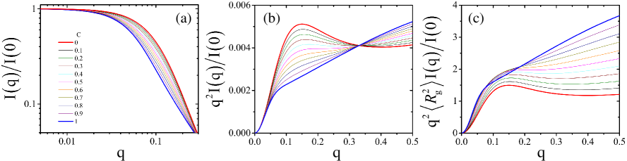
Figure S7: SAXS properties of the homogeneous ($C=0,1$) and composite ($C\neq 0,1$) ensembles with $\epsilon_{\rm p}^{(1)}=+2.0$ and $\epsilon_{\rm p}^{(2)}=-2.0$ in Fig. 21 of the main text. The color code for different $C$ values is identical to that in the main-text figure.

References

- (1) Sosnick, T. R.; Trewhella, J. Denatured states of ribonuclease A have compact dimensions and residual secondary structure. Biochemistry 1992, 31, 8329–8335.
- (2) Zhang, O.; Forman-Kay, J. D. Structural characterization of folded and unfolded states of an SH3 domain in equilibrium in aqueous buffer. Biochemistry 1995, 34, 6784–6794.
- (3) Plaxco, K. W.; Millet, I. S.; Segel, D. J.; Doniach, S.; Baker, D. Polypeptide chain collapse can occur concomitantly with the rate limiting step in protein folding. Nat. Struct. Biol. 1999, 6, 554–557.
- (4) Shortle, D.; Ackerman, M. S. Persistence of native-like topology in a denatured protein in 8 M urea. Science 2001, 293, 487–489.
- (5) Shimizu, S.; Chan, H. S. Origins of protein denatured state compactness and hydrophobic clustering in aqueous urea: Inferences from nonpolar potentials of mean force. Proteins 2002, 49, 560–566.
- (6) Jacob, J.; Krantz, B.; Dothager, R. S.; Thiyagarajan, P.; Sosnick, T. R. Early collapse is not an obligate step in protein folding. J. Mol. Biol. 2004, 338, 369–382.
- (7) Kohn, J. E.; Millett, I. S.; Jacob, J.; Zagrovic, B.; Dillon, T. M.; Cingel, N.; Dothager, R. S.; Seifert, S.; Thiyagarajan, P.; Sosnick, T. R.; Hasan, M. Z.; Pande, V. S.; Ruczinski, I.; Doniach, S.; Plaxco, K. W. Random-coil behavior and the dimensions of chemically unfolded proteins. Proc. Natl. Acad. Sci. U.S.A. 2004, 101, 12491–12496.
- (8) Fitzkee, N. C.; Rose, G. D. Reassessing random-coil statistics in unfolded proteins. Proc. Natl. Acad. Sci. U.S.A. 2004, 101, 12497–12502.
- (9) Sherman, E.; Haran, G. Coil-globule transition in the denatured state of a small protein. Proc. Natl. Acad. Sci. U.S.A. 2006, 103, 11539–11543.
- (10) Merchant, K. A.; Best, R. B.; Louis, J. M.; Gopich, I. V.; Eaton, W. A. Characterizing the unfolded states of proteins using single-molecule FRET spectroscopy and molecular simulations. Proc. Natl. Acad. Sci. U.S.A. 2007, 104, 1528–1533.
- (11) Marsh, J. A.; Forman-Kay, J. D. Structure and disorder in an unfolded state under nondenaturing conditions from ensemble models consistent with a large number of experimental restraints. J. Mol. Biol. 2009, 391, 359–374.
- (12) Meng, W.; Lyle, N.; Luan, B.; Raleigh, D. P.; Pappu, R. V. Experiments and simulations show how long-range contacts can form in expanded unfolded proteins with negligible secondary structure. Proc. Natl. Acad. Sci. U.S.A. 2013, 110, 2123–2128.
- (13) Stenzoski, N. E.; Luan, B.; Holehouse, A. S.; Raleigh, D. P. The unfolded state of the C-terminal domain of L9 expands at low but not at elevated temperatures. Biophys. J. 2018 115, 655–663.
- (14) Borg, M.; Mittag, T.; Pawson, T.; Tyers, M.; Forman-Kay, J. D.; Chan, H. S. Polyelectrostatic interactions of disordered ligands suggest a physical basis for ultrasensitivity. Proc. Natl. Acad. Sci. U.S.A. 2007, 104, 9650–9655.
- (15) Mittag, T.; Orlicky, S.; Choy, W.-Y.; Tang, X.; Lin, H.; Sicheri, F.; Kay, L. E.; Tyers, M.; Forman-Kay, J. D. Dynamic equilibrium engagement of a polyvalent ligand with a single-site receptor. Proc. Natl. Acad. Sci. U.S.A. 2008, 105, 17772–17777.
- (16) Müller-Späth, S.; Soranno, A.; Hirschfeld, V.; Hofmann, H.; Rüegger, S.; Reymond, L.; Nettels, D.; Schuler, B. Charge interactions can dominate the dimensions of intrinsically disordered proteins. Proc. Natl. Acad. Sci. U.S.A. 2010, 107, 14609–14614.
- (17) Mittag, T., Marsh, J.; Grishaev, A.; Orlicky, S.; Lin, H.; Sicheri, F.; Tyers, M.; Forman-Kay, J. D. Structure/function implications in a dynamic complex of the intrinsically disordered Sic1 with the Cdc4 subunit of an SCF ubiquitin ligase. Structure 2010, 18, 494–506.
- (18) Fuxreiter, M.; Tompa, P. Fuzzy complexes: a more stochastic view of protein function. Adv. Exp. Med. Biol. 2012, 725, 1–14.
- (19) Marsh, J. A.; Teichmann, S. A.; Forman-Kay, J. D. Probing the diverse landscape of protein flexibility and binding. Curr. Opin. Struct. Biol. 2012, 22, 643–650.
- (20) Liu, B.; Chia, D.; Csizmok, V.; Farber, P.; Forman-Kay, J. D.; Gradinaru, C. C. The effect of intrachin electrostatic repulsion on conformational disorder and dynamics of the Sic1 protein. J. Phys. Chem. B 2014, 118, 4088–4097.
- (21) Martin, E. W.; Holehouse, A. S.; Grace, C. R.; Hughes, A.; Pappu, R. V.; Mittag, T. Sequence determinants of the conformational properties of an intrinsically disordered protein prior to and upon multisite phosphorylation. J. Am. Chem. Soc. 2016, 138, 15323–15335.
- (22) Li, M.; Liu, Z. Dimensions, energetics, and denaturant effects of the protein unstructured state. Protein Sci. 2016, 25, 734–747.
- (23) Li, M.; Sun, T.; Jin, F.; Yu, D.; Liu, Z. Dimension conversion and scaling of disordered protein chains. Mol. Biosyst. 2016, 12, 2932–2940.
- (24) Holehouse, A. S.; Pappu, R. V. Collapse transitions of proteins and the interplay among backbone, sidechain, and solvent interactions. Annu. Rev. Biophys. 2018, 47, 19–39.
- (25) Chan, H. S.; Shimizu, S.; Kaya, H. Cooperativity principles in protein folding. Methods Enzymol. 2004, 380, 350–379.
- (26) Huang, F.; Ying, L.; Fersht, A. R. Direct observation of barrier-limited folding of BBL by single-molecule fluorescence resonance energy transfer. Proc. Natl. Acad. Sci. U.S.A. 2009, 106, 16239–16244.
- (27) Chan, H. S.; Zhang, Z.; Wallin, S.; Liu, Z. Cooperativity, local-nonlocal coupling, and nonnative interactions: Principles of protein folding from coarse-grained models. Annu. Rev. Phys. Chem. 2011, 62, 301–326.
- (28) Liu, J.; Campos, L. A.; Cerminara, M.; Wang, X.; Ramanathan, R.; English, D. S.; Muñoz, V. Exploring one-state downhill protein folding in single molecules. Proc. Natl. Acad. Sci. U.S.A. 2012, 109, 179–184.
- (29) Chen, T.; Chan, H. S. Effects of desolvation barriers and sidechains on local-nonlocal coupling and chevron behaviors in coarse-grained models of protein folding. Phys. Chem. Chem. Phys. 2014, 16, 6460–6479.
- (30) Maity, H.; Reddy, G. Folding of Protein L with implications for collapse in the denatured state ensemble. J. Am. Chem. Soc. 2016, 138, 2609–2616.
- (31) Thirumalai, D.; Samanta, H. S.; Maity, H.; Reddy, G. Universal nature of collapsibility in the context of protein folding and evolution. Trends Biochem. Sci. 2019, 44, 675–687.
- (32) Shoemaker, B. A.; Portman, J. J.; Wolynes, P. G. Speeding molecular recognition by using the folding funnel: The fly-casting mechanism. Proc. Natl. Acad. Sci. U.S.A. 2000, 97, 8868–8873.
- (33) Huang, Y.; Liu, Z. Kinetic advantage of intrinsically disordered proteins in coupled folding-binding process: a critical assessment of the “fly-casting” mechanism. J. Mol. Biol. 2009, 393, 1143–1159.
- (34) Csizmok, V.; Orlicky, S.; Cheng, J.; Song, J.; Bah, A.; Delgoshaie, N.; Lin, H.; Mittag, T.; Sicheri, F.; Chan, H. S.; Tyers, M.; Forman-Kay, J. D. An allosteric conduit facilitates dynamic multisite substrate recognition by the SCFCdc4 ubiquitin ligase. Nat. Comm. 2017, 8, 13943.
- (35) Sigalov, A. B.; Zhuravleva, A. V.; Orekhov, V. Yu. Binding of intrinsically disordered proteins is not necessarily accompanied by a structural transition to a folded form. Biochimie 2007, 89, 419–421.
- (36) Danielsson, J.; Liljedahl, L.; Bárány-Wallje, L.; Sønderby, P.; Kristensen, L. H.; Martinez-Yamout, M. A.; Dyson, H. J.; Wright, P. E.; Poulsen, F. M.; Mäler, L.; Gräslund, A.; Kragelund, B. B. The intrinsically disordered RNR inhibitor Sml1 is a dynamic dimer. Biochemistry 2008, 47, 13428–13437.
- (37) Nourse, A.; Mittag, T. The cytoplasmic domain of the T-cell receptor zeta subunit does not form disordered dimers. J. Mol. Biol., 2014, 426, 62–70.
- (38) Sigalov, A. B. Structural biology of intrinsically disordered proteins: Revisiting unsolved mysteries. Biochimie, 2016, 125, 112–118.
- (39) Wu, S.; Wang, D.; Liu, J.; Feng, Y.; Weng, J;.; Li, Y.; Gao, X.; Liu, J.; Wang, W. The dynamic multisite interactions between two intrinsically disordered proteins. Angew. Chem. Int. Ed. 2017, 56, 7515—7519.
- (40) Amin, A. N.; Lin, Y.-H.; Das, S.; Chan, H. S. Analytical theory for sequence-specific binary fuzzy complexes of charged intrinsically disordered proteins. J. Phys. Chem. B 2020, 124, 6709–6720.
- (41) Shin, Y.; Brangwynne, C.P. Liquid phase condensation in cell physiology and disease. Science 2017, 357, eaaf4382.
- (42) Banani, S. F.; Lee, H. O.; Hyman, A. A.; Rosen, M. K. Biomolecular condensates: organizers of cellular biochemistry. Nat. Rev. Mol. Cell Biol. 2017, 18, 285–298.
- (43) Lin, Y.-H.; Forman-Kay, J. D.; Chan, H. S. Theories for sequence-dependent phase behaviors of biomolecular condensates. Biochemistry 2018, 57, 2499–2508.
- (44) Lin, Y.-H.; Chan, H. S. Phase separation and single-chain compactness of charged disordered proteins are strongly correlated. Biophys, J. 2017, 112, 2043–2046.
- (45) Dignon, G. L.; Zheng, W.; Best, R. B.; Kim, Y. C.; Mittal, J. Relation between single-molecule properties and phase behavior of intrinsically disordered proteins. Proc. Natl. Acad. Sci. U.S.A. 2018, 115, 9929–9934.
- (46) McCarty, J.; Delaney, K. T.; Danielsen, S. P. O.; Fredrickson, G. H.; Shea, J.-E. Complete phase diagram for liquid-liquid phase separation of intrinsically disordered proteins. J. Phys. Chem. Lett. 2019, 10, 1644–1652.
- (47) Zeng, X.; Holehouse, A. S.; Mittag, T.; Chilkoti, A.; Pappu, R. V. Connecting coil-to-globule transitions to full phase diagrams for intrinsically disordered proteins. Biophys. J. 2020, 119, 402–418.
- (48) Piana, S.; Klepeis, J. L.; Shaw, D. E. Assessing the accuracy of physical models used in protein-folding simulations: Quantitative evidence from long molecular dynamics simulations. Curr. Opin. Struct. Biol. 2014, 24, 98–105.
- (49) Chen, T.; Song, J.; Chan, H. S. Theoretical perspectives on nonnative interactions and intrinsic disorder in protein folding and binding. Curr. Opin. Struct. Biol. 2015, 30, 32–42.
- (50) Rauscher, S.; Gapsys, V.; Gajda, M. J.; Zweckstetter, M.; de Groot, B. L.; Grubmüller, H. Structural ensembles of intrinsically disordered proteins depend strongly on force field: A comparison to experiment. J. Chem. Theor. Comput. 2015, 11, 5513–5524.
- (51) Huang, J.; Rauscher, S.; Nawrocki, G.; Ran, T.; Feig, M.; de Groot, B. L.; Grubmüller, H.; MacKerell, A. D. Jr. CHARMM36m: An improved force field for folded and intrinsically disordered proteins. Nat. Methods 2017 14, 71–73.
- (52) Best, R. B. Computational and theoretical advances in studies of intrinsically disordered proteins. Curr. Opin. Struct. Biol. 2017, 42, 147–154.
- (53) Levine, Z. A.; Shea, J.-E. Simulations of disordered proteins and systems with conformational heterogeneity. Curr. Opin. Struct. Biol. 2017, 43, 95–103.
- (54) Robustelli, P.; Piana, S.; Shaw, D. E. Developing a molecular dynamics force field for both folded and disordered protein states. Proc. Natl. Acad. Sci. U.S.A. 2018, 115, E4758–E4766.
- (55) Shea, J.-E.; Best, R. B.; Mittal, J. Physics-based computational and theoretical approaches to intrinsically disordered proteins. Curr. Opin. Struct. Biol. 2021, 67, 219–225.
- (56) Doniach, S. Changes in biomolecular conformation seen by small angle X-ray scattering. Chem. Rev. 2001, 101, 1763–1778.
- (57) Schindler, C. E. M.; de Vries, S. J.; Sasse, A.; Zacharias, M. SAXS data alone can generate high-quality models of protein-protein complexes. Structure 2016, 24, 1387–1397.
- (58) Meisburger, S. P.; Thomas, W. C.; Watkins, M. B.; Ando, N. X-ray scattering studies of protein structural dynamics. Chem. Rev. 2017, 117, 7615–7672.
- (59) Yoo, T. Y.; Meisburger, S. P.; Hinshaw, J.; Pollack, L.; Haran, G.; Sosnick, T. R.; Plaxco, K. Small-angle x-ray scattering and single-molecule FRET spectroscopy produce highly divergent views of the low-denaturant unfolded state. J. Mol. Biol. 2012, 418, 226–236.
- (60) Kathuria, S. V.; Kayatekin, C.; Barrea, R.; Kondrashkina, E.; Graceffa, R.; Guo, L.; Nobrega, R. P.; Chakravarthy, S.; Matthews, C. R.; Irving, T. C.; Bilsel, O. Microsecond barrier-limited chain collapse observed by time-resolved FRET and SAXS. J. Mol. Biol. 2014, 426, 1980–1994.
- (61) Kikhney, A. G.; Svergun, D. I. A practical guide to small angle X-ray scattering (SAXS) of flexible and intrinsically disordered proteins. FEBS Lett. 2015, 589, 2570–2577.
- (62) Watkins, H. M.; Simon, A. J.; Sosnick, T. R.; Lipman, E. A.; Hjelm, R. P.; Plaxco, K. W. Random coil negative control reproduces the discrepancy between scattering and FRET measurements of denatured protein dimensions. Proc. Natl. Acad. Sci. U.S.A. 2015, 112, 6631–6636.
- (63) Antonov, L. D.; Ollsson, S.; Boomsma, W.; Hamelryck, T. Bayesian inference of protein ensembles from SAXS data. Phys. Chem. Chem. Phys. 2016, 18, 5832–5838.
- (64) Aznauryan, M.; Delgado, L.; Soranno, A.; Nettels, D. ; Huang, J.; Labhardt, A. M.; Grzesiek, S.; Schuler, B. Comprehensive structural and dynamical view of an unfolded protein from the combination of single-molecule FRET, NMR, and SAXS. Proc. Natl. Acad. Sci. U.S.A. 2016, 113, E5389–E5398.
- (65) Martin, E. W.; Hopkins, J. B.; Mittag, T. Small-angle X-ray scattering experiments of monodisperse intrinsically disordered protein samples close to the solubility limit. Methods Enzymol. 2021, 646, 185–222.
- (66) Haran, G. How, when and why protein collapse: The relation to folding. Curr. Opin. Struct. Biol. 2012, 22, 14–20.
- (67) Schuler, B.; Hofmann, H. Single-molecule spectroscopy of protein folding dynamics—expanding scope and timescales. Curr. Opin. Struct. Biol. 2013, 23, 36–47.
- (68) Juette, M. F.; Terry, D. S.; Wasserman, M. R.; Zhou, Z.; Altman, R. B.; Zheng, Q.; Blanchard, S. C. The bright future of single-molecule fluorescence imaging. Curr. Opin. Struct. Biol. 2014, 20, 103–111.
- (69) Elbaum-Garfinkle, S.; Cobb, G.; Compton, J. T.; Li, X.-H.; Rhoades E. Tau mutants bind tubulin heterodimers with enhanced affinity. Proc. Natl. Acad. Sci. U.S.A. 2014, 111, 6311–6316.
- (70) Banerjee, P. R.; Deniz, A, A. Shedding light on protein folding landscapes by single-molecule fluorescence. Chem. Soc. Rev. 2014, 43, 1172–1188.
- (71) König, I.; Zarrine-Afsar, A.; Aznauryan, M.; Soranno, A.; Wunderlich, B.; Dingfelder, F.; Stüber, J. C.; Plückthun, A.; Nettels, D.; Schuler, B. Single-molecule spectroscopy of protein conformational dynamics in live eukaryotic cells. Nature Methods 2015, 12, 773–779.
- (72) Melo, A. M.; Coraor, J.; Alpha-Cobb, G.; Elbaum-Garfinkle, S.; Nath, A.; Rhoades, E. A functional role for intrinsic disorder in the tau-tubulin complex. Proc. Natl. Acad. Sci. U.S.A. 2016, 113, 14336–14341.
- (73) Schuler, B., Soranno, A.; Hofmann, H.; Nettels, D. Single-molecule FRET spectroscopy and the polymer physics of unfolded and intrinsically disordered proteins. Annu. Rev. Biophys. 2016, 45, 207–231.
- (74) O’Brien, E. P.; Morrison, G.; Brooks, B. R.; Thirumalai, D. How accurate are polymer models in the analysis of Förster resonance energy transfer experiments on proteins? J. Chem. Phys. 2009, 130, 124903.
- (75) Hofmann, H.; Nettels, D.; Schuler, B. Single-molecule spectroscopy of the unexpected collapse of an unfolded protein at low pH. J. Chem. Phys. 2013, 139, 121930.
- (76) Song, J.; Gomes, G.-N.; Gradinaru, C. C.; Chan, H. S. An adequate account of excluded volume is necessary to infer compactness and asphericity of disordered proteins by Förster resonance energy transfer. J. Phys. Chem. B 2015, 119, 15191–15202.
- (77) Song, J.; Gomes, G.-N.; Shi, T.; Gradinaru, C. C.; Chan, H. S. Conformational heterogeneity and FRET data interpretation for dimenions of unfolded proteins. Biophys. J. 2017, 113, 1012–1024.
- (78) Fuertes, G.; Banterle, N.; Ruff, K. M.; Chowdhury, A.; Mercadante, D.; Koehler, C.; Kachala, M.; Girona, G. E.; Milles, S.; Mishra, A.; Onck, P. R.; Gräter, F.; Esteban-Martin, S.; Pappu, R. V.; Svergun, D. I.; Lemke, E. A. Dcoupling of size and shape fluctuations in heteropolymeric sequences reconciles discrepancies in SAXS versus FRET measurements. Proc. Natl. Acad. Sci. U.S.A. 2017, 114, E6342–E6351.
- (79) Peran, I.; Holehouse, A. S.; Carrico, I. S.; Pappu, R. V.; Bilsel, O.; Raleigh, D. P. Unfolded states under folding conditions accommodate sequence-specific conformational preferences with random coil-like dimensions. Proc. Natl. Acad. Sci. U.S.A. 2019, 116, 12301–12310.
- (80) Domb, C.; Gillis, J.; Wilmers, G. On the shape and configuration of polymer molecules. Proc. Phys. Soc. (London) 1965, 85, 625–645.
- (81) Fisher, M. E. Shape of a self-avoiding walk or polymer chain. J. Chem. Phys. 1966, 44, 616–622.
- (82) des Cloizeaux, J. Lagrangian theory for a self-avoiding random chain. Phys. Rev. A 1974, 10, 1665–1669.
- (83) Oono, Y.; Ohta, T.; Freed, K. F. Application of dimensional regularization to single chain polymer static properties: Conformational space renormalization of polymers. III. J. Chem. Phys. 1981, 74, 6458–6466.
- (84) Zheng, W.; Zerze, G. H.; Borgia, A.; Mittal, J.; Schuler, B.; Best, R. B. Inferring properties of disordered chains from FRET transfer efficiencies. J. Chem. Phys. 2018, 148, 123329.
- (85) Zheng, W.; Best, R. B. An extended guinier analysis for intrinsically disordered proteins. J. Mol. Biol. 2018, 430, 2540–2553.
- (86) Vendruscolo, M. Determination of conformationally heterogeneous states of proteins. Curr. Opin. Struct. Biol. 2007, 17, 15–20.
- (87) Lyle, N.; Das, R. K.; Pappu, R. V. A quantitative measure for protein conformational heterogeneity. J. Chem. Phys. 2013, 139, 121907.
- (88) Ruff, K. M.; Holehouse, A. S. SAXS versus FRET: A matter of heterogeneity? Biophys. J. 2017, 113, 971–973.
- (89) Best, R. B. Emerging consensus on the collapse of unfolded and intrinsically disordered proteins in water. Curr. Opin. Struct. Biol. 2020, 60, 27–38.
- (90) Mazouchi, A.; Zhang, Z.; Bahram, A.; Gomes, G.-N.; Lin, H.; Song, J.; Chan, H. S.; Forman-Kay, J. D.; Gradinaru, C, C. Conformations of a metastable SH3 domain characterized by smFRET and an excluded-volume polymer model. Biophys. J. 2016, 110, 1510–1522.
- (91) Gomes, G.-N.; Gradinaru, C. C. Insights into the conformations and dynamics of intrinsically disordered proteins using single-molecular fluorescence. Biochim. Biophys. Acta 2017, 1865, 1696–1706.
- (92) Gomes, G.-N. W.; Krzeminski, M.; Namini, A.; Martin, E. W.; Mittag, T.; Head-Gordon, T.; Forman-Kay, J. D.; Gradinaru, C. C. Conformational ensembles of an intrinsically disordered protein consistent with NMR, SAXS, and single-molecule FRET. J. Am. Chem. Soc. 2020, 142, 15697–15710.
- (93) Riback, J. A.; Bowman, M. A.; Zmyslowski, A. M.; Knoverek. C. R.; Jumper, J. M.; Hinshaw, J. R.; Kaye, E. B.; Freed, K. F.; Clark P. L.; Sosnick, T. R. Innovative scattering analysis shows that hydrophobic disordered proteins are expanded in water. Science 2017, 358, 238–241.
- (94) Best, R. B.; Zheng, W.; Borgia, A.; Buholzer, K.; Borgia, M. B.; Hofmann, H.; Soranno, A.; Nettels, D.; Gast, K.; Grishaev, A.; Schuler, B. Comment on “Innovative scattering analysis shows that hydrophobic disordered proteins are expanded in water”. Science 2018, 361, eaar7101.
- (95) Riback, J. A.; Bowman, M. A.; Zmyslowski, A. M.; Knoverek. C. R.; Jumper, J. M.; Kaye, E. B.; Freed, K. F.; Clark P. L.; Sosnick, T. R. Response to comment on “Innovative scattering analysis shows that hydrophobic disordered proteins are expanded in water”. Science 2018, 361, eaar7949.
- (96) Fuertes, G.; Banterie, N.; Ruff, K. M.; Chowdhury, A.; Pappu, R. V.; Svergun, D. I.; Lemke, E. A. Comment on “Innovative scattering analysis shows that hydrophobic disordered proteins are expanded in water”. Science 2018, 361, eaar8230.
- (97) Gradinaru Lab and Chan Lab. DICE (Dimensional Inferences from Coarse-grained Ensembles), 2017. University of Toronto. http://dice.utm.utoronto.ca/
- (98) Stenzoski, N. E.; Zou, J.; Piserchio, A.; Ghose, R.; Holehouse, A. S.; Raleigh, D. P. The cold-unfolded state is expanded but contains long- and medium-range contacts and is poorly described by homopolymer models. Biochemistry 2020, 59, 3290–3299.
- (99) Fixman, M. Excluded volume in polymer chains. J. Chem. Phys. 1955, 23, 1656–1659.
- (100) Fixman, M. Radius of gyration of polymer chains. J. Chem. Phys. 1962, 36, 306–310.
- (101) Fixman, M. Radius of gyration of polymer chains. II. Segment density and excluded volume effects. J. Chem. Phys. 1962, 36, 3123–3129.
- (102) Edwards, S. F. The statistical mechanics of polymers with excluded volume. Proc. Phys. Soc. 1965, 85, 613–624.
- (103) Yamakawa, H.; Aoki, A.; Tanaka, G. Second-order perturbation theory of the mean-square radius of a linear polymer molecule. J. Chem. Phys. 1966, 45, 1938–1941.