Entrywise Estimation of Singular Vectors of Low-Rank Matrices with Heteroskedasticity and Dependence

Abstract

We propose an estimator for the singular vectors of high-dimensional low-rank matrices corrupted by additive subgaussian noise, where the noise matrix is allowed to have dependence within rows and heteroskedasticity between them. We prove finite-sample $\ell_{2,\infty}$ bounds and a Berry-Esseen theorem for the individual entries of the estimator, and we apply these results to high-dimensional mixture models. Our Berry-Esseen theorem clearly shows the geometric relationship between the signal matrix, the covariance structure of the noise, and the distribution of the errors in the singular vector estimation task. These results are illustrated in numerical simulations. Unlike previous results of this type, which rely on assumptions of Gaussianity or independence between the entries of the additive noise, handling the dependence between entries in the proofs of these results requires careful leave-one-out analysis and conditioning arguments. Our results depend only on the signal-to-noise ratio, the sample size, and the spectral properties of the signal matrix.

Keywords: Entrywise estimation, singular vectors, heteroskedastic, Berry-Esseen

1 Introduction

Consider the signal-plus-noise model

$$\widehat{M}=M+E,$$

where $M\in\mathbb{R}^{n\times d}$ is a deterministic rank $r$ signal matrix and $E$ is a mean-zero noise matrix. We assume $M$ has the singular value decomposition

$$M=U\Lambda V^{\top},$$

where $U$ is an $n\times r$ matrix with orthonormal columns, $\Lambda$ is an $r\times r$ diagonal matrix whose entries are the $r$ nonzero singular values $\lambda_{1}\geq\lambda_{2}\geq\cdots\geq\lambda_{r}>0$ of $M$, and $V$ is an $d\times r$ matrix with orthonormal columns. Letting $E_{i}^{\top}$ denote the $i$’th row of the noise matrix $E$, we suppose each noise vector $E_{i}$ is of the form

$$E_{i}=\Sigma_{i}^{1/2}Y_{i},$$

where $\mathbb{E}Y_{i}=0$, $\Sigma_{i}\in\mathbb{R}^{d\times d}$ is a positive semidefinite matrix allowed to depend on the row $i$, and the coordinates $Y_{i\alpha}$ of the vector $Y_{i}$ are independent subgaussian random variables satisfying $\mathbb{E}Y_{i\alpha}^{2}=1$. Define the signal to noise ratio

$$\mathrm{SNR}:=\frac{\lambda_{r}}{\sigma\sqrt{rd}},$$

where $\sigma^{2}:=\max_{i}\|\Sigma_{i}\|$ is the maximum spectral norm of the covariances of each row.

In this work we study the entrywise estimation of the matrix $U$ (or column space of $M$) in the “quasi-asymptotic regime” wherein $n$ and $d$ are assumed to be large but finite. Because we allow the rows of $E$ to have different covariances, the “vanilla SVD” can be biased, so we propose a bias-corrected estimator for the matrix $U$ and analyze its limiting distribution when the signal to noise ratio is large enough relative to the dimension of the problem. Furthermore, we do not assume distinct singular values for $M$.

Our main contributions are the following:

• We provide a nonasymptotic Berry-Esseen Theorem (Theorem 1) for the entries of our proposed estimator for $U$ under general assumptions on the signal matrix $M$ and the noise matrix $E$;

• We study the $\ell_{2,\infty}$ approximation (Theorem 2) of our proposed estimator to $U$ which matches previous $\ell_{2,\infty}$ bounds in the special case of independent noise.

• We apply our results to the particular setting of a $K$-component subgaussian mixture model (Corollary 2) and show that one can accurately estimate the resulting limiting covariance of the rows of our estimator within each community (Corollary 3), allowing us to derive data-driven, asymptotically valid confidence regions.

Since we allow for dependence within each row of the noise matrix $E$, our asymptotic results highlight the geometric relationship between the covariance structure and the singular subspaces of $M$. Furthermore, our estimator is based off the HeteroPCA algorithm proposed in Zhang et al. (2021), so as a byproduct of our results, we also provide a more refined analysis of this algorithm, leading to an upper bound on the $\ell_{2,\infty}$ error that scales with the noise.

The organization of the paper is as follows. In the next subsection we discuss related work, and we end this section with notation and terminology we will use throughout. In Section 2, we recall the HeteroPCA algorithm of Zhang et al. (2021), and use this to define our estimator $\widehat{U}$ for $U$. We also discuss alternative approaches to the problem and some of the shortcomings of those approaches which have motivated the present work. In Section 3, we state our main theorems, namely our $\ell_{2,\infty}$ concentration and Berry-Esseen theorems. We also discuss the various assumptions of our model, and compare these to previous work. In Section 3.2, we discuss the statistical implications of our results for mixture distributions. We further illustrate our results in simulations in Section 4. Discussion of these results and potential future work is in Section 5. Finally, Section 6 contains the proof of Theorem 2 and a proof sketch of Theorem 1. The full proof of Theorem 1 and additional supplementary lemmas are contained in the Appendices.

1.1 Related Work

Spectral methods, which refer to a collection of tools and techniques informed by matrix analysis and eigendecompositions, underpin a number of methods used in high-dimensional multivariate statistics and data science, including but not limited to network analysis (Abbe et al., 2020a, b; Agterberg et al., 2020; Athreya et al., 2017; Cai et al., 2020; Fan et al., 2019; Jin et al., 2019; Lei, 2019; Lei and Rinaldo, 2015; Mao et al., 2020; Rubin-Delanchy et al., 2020; Zhang et al., 2020), principal components analysis, (Cai et al., 2020; Cai and Zhang, 2018; Cai et al., 2021; Koltchinskii et al., 2020; Koltchinskii and Lounici, 2017; Koltchinskii and Xia, 2016; Koltchinskii and Lounici, 2016; Wang and Fan, 2017; Johnstone and Lu, 2009; Lounici, 2013, 2014; Xie et al., 2019; Zhu et al., 2019), and spectral clustering (Abbe et al., 2020a, b; Amini and Razaee, 2021; Cai et al., 2020; Lei, 2019; Löffler et al., 2020; Schiebinger et al., 2015; Srivastava et al., 2021). In addition, eigenvectors or related quantities can be used as a “warm start” for optimization methods (Chen et al. (2019, 2021b); Chi et al. (2019); Lu and Li (2017); Ma et al. (2020); Xie and Xu (2020); Xie (2021)), yielding provable convergence to quantities of interest provided the initialization is sufficiently close to the optimum. The model we consider includes as a submodel the high-dimensional $K$-component mixture model. High-Dimensional mixture models play an important role in the analysis of spectral clustering (Abbe et al., 2020a; Amini and Razaee, 2021; Löffler et al., 2020; Schiebinger et al., 2015; Vempala and Wang, 2004; von Luxburg, 2007) and classical multidimensional scaling (Ding and Sun, 2019; Li et al., 2020; Little et al., 2020).

To analyze these methods, researchers have used existing results on matrix perturbation theory such as the celebrated Davis-Kahan $\sin\Theta$ Theorem (Bhatia, 1997; Yu et al., 2014; Chen et al., 2021b), which provides a deterministic bound on the difference between the eigenvectors of a perturbed matrix and the eigenvectors of the unperturbed matrix, provided the perturbation is sufficiently small. Unfortunately, the Davis-Kahan Theorem and classical approaches to matrix perturbation analysis may fail to provide entrywise guarantees for estimated eigenvectors, though there has been work on studying the subspace distances in the presence of random noise (Li and Li, 2018; Xia, 2019b; Bao et al., 2021; O’Rourke et al., 2018; Ding, 2020).

Entrywise eigenvector analysis plays an important role in furthering the understanding of spectral methods in a number of statistical problems (Abbe et al., 2020b, a; Cai et al., 2020; Cape et al., 2019a, b; Chen et al., 2021b; Damle and Sun, 2019; Eldridge et al., 2018; Fan et al., 2018; Lei, 2019; Luo and Zhang, 2020; Mao et al., 2020; Rohe and Zeng, 2020; Xia and Yuan, 2020; Xie et al., 2019; Zhong and Boumal, 2018; Zhu et al., 2019). A number of works have studied entrywise eigenvector or singular vector analysis when the noise matrix $E$ consists of independent entries (Abbe et al., 2020b, a; Chen et al., 2021b; Cape et al., 2019a; Cai et al., 2020; Lei, 2019), and some authors have also studied the estimation of linear forms of eigenvectors (Chen et al., 2021a; Cheng et al., 2020; Fan et al., 2020; Koltchinskii and Xia, 2016; Koltchinskii and Lounici, 2017; Koltchinskii and Xia, 2016; Koltchinskii, 1998; Koltchinskii et al., 2020; Li et al., 2021). In the present work, we extend existing results on entrywise analysis by allowing for dependence in the noise matrix. We address this more general setting using a combination of matrix series expansions (Cape et al., 2019a; Chen et al., 2021a; Eldridge et al., 2018; Xia, 2019a, b; Xia and Yuan, 2020; Xie et al., 2019), leave-one-out analysis (Abbe et al., 2020b, a; Chen et al., 2021b; Lei, 2019), and careful conditioning arguments.

While entrywise statistical guarantees refine classical deterministic perturbation techniques, they do not necessarily allow for studying the distributional properties of the eigenvectors. Several works have studied the asymptotic distributions of individual eigenvectors (Cape et al., 2019a; Fan et al., 2020) or $\sin\Theta$ distances (Bao et al., 2021; Ding, 2020; Li and Li, 2018; Xia, 2019b), but there are very few finite-sample results on the distribution of the individual entries of singular vectors rather than eigenvectors, and existing results often depend on independence of the noise. We explicitly characterize the distribution of the individual entries of the estimated singular vectors, which showcases the effect that the geometric relationship of the covariance structure of the rows of $E$ and the spectral structure of the signal matrix $M$ has on this distribution.

Finally, the bias of the singular value decomposition in the presence of heteroskedastic noise has been addressed in a number of works (Cai et al., 2020; Abbe et al., 2020a; Florescu and Perkins, 2016; Koltchinskii and Giné, 2000; Leeb and Romanov, 2021; Lei and Lin, 2021; Lounici, 2014). A common method for addressing this is the diagonal deletion algorithm, for which an entrywise analysis is carried out in Cai et al. (2020) for several different statistical problems. However, as identified in Zhang et al. (2021), in some situations diagonal deletion incurs unnecessary additional error, leading them to propose the HeteroPCA algorithm which we further study here. We include detailed comparisons to existing work in Section 3.

1.2 Notation

We use capital letters for both matrices and vectors, where the distinction will be clear from context, except for the letter $C$, which we use to denote constants. For a matrix $M$, we write $M_{ij}$ as its $i,j$ entry, $M_{\cdot j}$ for its $j$’th column and $M_{j\cdot}$ for its $j$’th row. The symbol $e_{i}$ represents the standard basis vector in the appropriate dimension. We use $\|\cdot\|$ to denote the spectral norm for matrices and the Euclidean norm for vectors, and $\|\cdot\|_{F}$ as the Frobenius norm for matrices. We write the $\ell_{2,\infty}$ norm of a matrix as $\|U\|_{2,\infty}=\max_{i}\|U_{i\cdot}\|$ which is the maximum Euclidean row norm. We consider the set of orthogonal $r\times r$ matrices as $\mathbb{O}(r)$, and we exclusively use the letter $\mathcal{O}$ to mean an element of $\mathbb{O}(r)$. We write $\langle\cdot,\cdot\rangle$ as the standard Euclidean inner product.

For a random variable $X$ taking values in $\mathbb{R}$, we let $\|X\|_{\psi_{2}}$ denote its $\psi_{2}$ (subgaussian) Orlicz norm; that is,

$$\|X\|_{\psi_{2}}:=\sup_{z\in\mathbb{R}}\{\mathbb{E}\exp(X^{2}/z)\leq 2\},$$

and for a random variable $Y$ taking values in $\mathbb{R}^{d}$, we let $\|Y\|_{\psi_{2}}$ denote $\sup\|\langle Y,u\rangle\|_{\psi_{2}}$, where the supremum is over all unit vectors $u$. Similarly we denote $\|\cdot\|_{\psi_{1}}$ as the $\psi_{1}$ (subexponential) Orlicz norm. For more details on relationships between these norms, see Vershynin (2018).

For two equal-sized matrices $U_{1}$ and $U_{2}$ with orthonormal columns, we denote the $\sin\Theta$ distance between them as

$$\|\sin\Theta(U_{1},U_{2})\|:=\|U_{1}U_{1}^{\top}-U_{2}U_{2}^{\top}\|.$$

For details on the $\sin\Theta$ distance between subspaces, see Bhatia (1997), Chen et al. (2021b), Cape et al. (2019b), or Cape (2020). For a square matrix $M$, we write $\Gamma(M)$ to be the hollowed version of $M$; that is, $\Gamma(M)_{ij}=M_{ij}$ for $i\neq j$ and $\Gamma(M)_{ii}=0$. We write $G(M):=M-\Gamma(M)$.

Occasionally we will write $f(n,d)\lesssim g(n,d)$ if there exists a constant $C$ sufficiently large such that $f(n,d)\leq Cg(n,d)$ for sufficiently large $n$ and $d$. We also write $f(n,d)\ll g(n,d)$ if $f(n,d)/g(n,d)$ tends to zero as $n$ and $d$ tend to infinity. We write $f(n,d)=O(g(n,d))$ if $f(n,d)\lesssim g(n,d)$. For two numbers $a$ and $b$, we write $a\vee b$ to denote the maximum of $a$ and $b$. Finally we write $f(n,d)\asymp g(n,d)$ if $f(n,d)=O(g(n,d))$ and $g(n,d)=O(f(n,d))$.

2 Background and Methodology

We consider a rectangular matrix $M\in\mathbb{R}^{n\times d}$ in the “high-dimensional regime” wherein $n$ and $d$ are large and comparable, though we are interested in the setting that $d$ is larger than $n$. We observe $\widehat{M}=M+E$ where the additive error matrix $E$ has rows $E_{i}^{\top}$ which are independent with covariance matrices $\Sigma_{i}\in\mathbb{R}^{d\times d}$ that are allowed to vary between rows. We write the singular value decomposition of $M$ as $U\Lambda V^{\top}$, where $U\in\mathbb{R}^{n\times r},V\in\mathbb{R}^{d\times r}$ are matrices with orthonormal columns and $\Lambda\in\mathbb{R}^{r\times r}$ is diagonal with nonincreasing positive diagonal entries $\lambda_{1}\geq\lambda_{2}\geq\cdots\geq\lambda_{r}>0$ that are not necessarily distinct. We note that this decomposition of $M$ is not unique, so we fix some choice of $U$, which necessarily fixes a choice of $V$ also. Our results account for the nonuniqueness of $U$ by aligning the estimator $\widehat{U}$ to $U$ through right-multiplication by an $r\times r$ orthogonal matrix. For more details on this alignment procedure, see, for example, Chen et al. (2021b) or Cape (2020).

0:  Input matrix $A+Z$, rank $r$, and maximum number of iterations $T$

1:  Let $N_{0}:=\Gamma(A+Z)$; $T=0$

2:  repeat

3:     Take SVD of $N_{T}:=\sum_{i}\lambda_{i}^{(T)}U_{\cdot i}^{(T)}(V_{\cdot i}^{(T)})^{\top}$

4:     Set $\tilde{N}_{T}:=\sum_{i\leq r}\lambda_{i}^{(T)}U_{\cdot i}^{(T)}(V_{\cdot i}^{(T)})^{\top}$ the best rank $r$ approximation of $N_{T}$

5:     Set $N_{T+1}:=G(\tilde{N}_{T})+\Gamma(N_{T})$

6:     $T=T+1$

7:  until convergence or maximum number of iterations reached

8:  return  $\widehat{U}:=U^{(T)}$

Algorithm 1 HeteroPCA (Algorithm 1 of Zhang et al. (2021))

Since $U$ may equivalently be understood to be the matrix of eigenvectors of $A=MM^{\top}$ corresponding to its $r$ nonzero eigenvalues, it is natural to consider $A$ and its noisy counterpart $A+Z,$ where $Z=ME^{\top}+EM^{\top}+EE^{\top}$, sometimes referred to as the “sample Gram matrix” in the literature (e.g. (Cai et al., 2020)). The matrix $\mathbb{E}[Z]$ is diagonal with diagonal entries $\text{Tr}(\Sigma_{i})$. When $d$ is large and the rows of $E$ are heteroskedastic, this means that the eigenvectors of $A+\mathbb{E}[Z]$ may not well-approximate those of $A$.

Authors have suggested hollowing the matrix $A+Z$ as a method to correct this bias, which amounts to using the eigenvectors of $\Gamma(A+Z)$ as the estimator for those of $A$. An analysis of this approach is given in Cai et al. (2020) and Abbe et al. (2020a), though this is not the primary focus of the latter. Unfortunately, while the eigenvectors of $\Gamma(A+Z)$ may be closer to the eigenvectors of $A$ than those of $A+Z$, they still incur a nontrivial, deterministic bias owing to the loss of information along the diagonal of $A$. In Zhang et al. (2021), the authors provide an example where the eigenvectors of $\Gamma(A+Z)$ do not yield a consistent estimator for $U$ in the regime that $n$ and $d$ tend to infinity with $d\asymp n$. This motivates their alternative approach to correcting the bias, the HeteroPCA algorithm, which we review in Algorithm 1. In essence, the algorithm proceeds by iteratively re-scaling the diagonals, attempting to fit the off-diagonal entries of $A+Z$ while maintaining the low rank $r$. We refer to the output of this algorithm after sufficiently many iterations as $\widehat{A}$ (see Theorem 1 for a quantitative condition on the number of iterations), and prove in Lemma 2 that it well-approximates the “idealized” perturbation of $A$ given by $\tilde{A}=A+\Gamma(Z)$ in spectral norm. This latter matrix has mean $A$, meaning that the bias along the diagonal has been accounted for. Removing this bias is also important for our distributional results, since otherwise one must center around the eigenvectors of $\Gamma(A)$ rather than those of $A$, but our interest is in the latter quantity.

The leading eigenvectors $\widehat{U}$ of this matrix $\widehat{A}$ serve as our estimator for $U$, and our concentration and distributional results demonstrate the quality of this estimator. This builds on the work in Zhang et al. (2021), where they prove a bound on the $\sin\Theta$ distance between $\widehat{U}$ and $U$, showing that $\widehat{U}$ is a consistent estimator for $U$. While a bound on the discrepancy between $\widehat{U}$ and $U$ in this metric is a first step towards the entrywise concentration results we obtain here, our results require much tighter control of the error between them. In addition, measuring the error in this way does not lend itself to the distributional results we consider in Theorem 1.

In the case that $M$ is well-conditioned and has highly incoherent singular vectors $U$ and $V$, the bias associated with diagonal deletion is not too severe, and the difference in performance between the eigenvectors of $\widehat{A}$ and $\Gamma(A+Z)$ may not be significant, especially when $n$ and $d$ are large. On the other hand, for moderate $n$ and $d$, or for moderate levels of incoherence in $U$ and $V$, the bias incurred by diagonal deletion is highly significant. We consider an example of this in Figure 1, in the setting of estimating memberships in a Gaussian mixture model, under heteroskedasticity and dependence. The noise level in this problem is relatively small, which suggests that consistent estimation should be possible for the right estimator, however the moderate incoherence causes a severe breakdown in the performance of the estimate obtained by diagonal deletion, while the HeteroPCA algorithm continues to perform well.

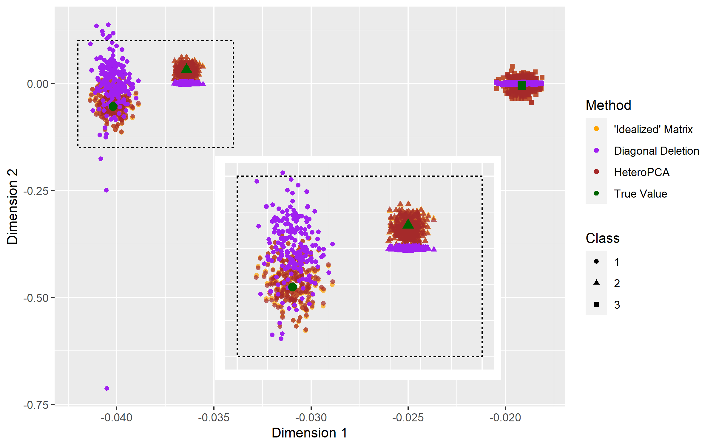
Figure 1: Comparison of the estimators for $U$ given by the eigenvectors of $\Gamma(A+Z)$ (diagonal deletion) and those of $\widehat{A}$ (the output of the HeteroPCA algorithm). For convenience, we also plot the eigenvectors of the “idealized” matrix $A+\Gamma(Z)$ that the HeteroPCA algorithm is approximating as well as a zoomed-in reference for classes one and two. For details on the experimental setup, see Section 4.

3 Main Results

Before presenting our main results, we discuss the various assumptions required, and their role in the analysis. Our first assumption concerns the noise matrix $E$.

Assumption 1 (Noise).

The noise matrix $E$ has rows $E_{i}^{\top}$ that can be written in the form $E_{i}=\Sigma_{i}^{1/2}Y_{i}$, where each $Y_{i}$ is a vector of independent mean-zero subgaussian random variables with unit variance and $\psi_{2}$ norm uniformly bounded by 1, and $\Sigma_{i}$ is positive semidefinite.

The following assumption ensures that there is sufficient signal to consistently identify the eigenvectors $U$. We let $\kappa:=\lambda_{1}/\lambda_{r}$ denote the condition number of $M$.

Assumption 2 (Enough Signal).

The signal-to-noise ratio satisfies $\mathrm{SNR}\geq C_{SNR}\kappa\sqrt{\log(n\vee d)}$, for a sufficiently large constant $C_{SNR}$.

We remark that in the case of independent noise, $\mathrm{SNR}\to\infty$ is required in order for consistency (e.g. Cai and Zhang (2018); Zhang et al. (2021); Xia (2019b)).

The following assumption ensures that we have sufficiently many samples for our concentration results to hold.

Assumption 3 (High Dimensional Regime, Low Rank).

There exists a constant $c_{1}$ and a sufficiently small constant $c_{2}$ such that such that $d\geq c_{1}n$, and $r\leq c_{2}n$. In addition, $\log(d)\leq n$.

The next assumption concerns the incoherence of the matrix $M$, which measures the “spikiness” of the matrix. We say $M$ is $\mu_{0}$-incoherent if

$$\max\bigg{\{}\|U\|_{2,\infty}\sqrt{\frac{n}{r}},\|V\|_{2,\infty}\sqrt{\frac{d}{r}}\bigg{\}}\leq\mu_{0}.$$

When $\mu_{0}=O(1)$, then the entries of $U$ and $V$ are spread, which corresponds to $M$ being fully incoherent. For more details, see (Chen et al., 2021b; Chi et al., 2019).

Assumption 4 (Incoherence).

The matrix $U$ of left singular vectors of $M$ satisfies $\|U\|_{2,\infty}\leq\mu_{0}\sqrt{\frac{r}{n}}$, where $\mu_{0}$ satisfies $\kappa^{2}\mu_{0}\leq\sqrt{n}$. In addition, there exists a constant $C_{I}$ sufficiently large such that $\|V\|_{2,\infty}\leq C_{I}\|U\|_{2,\infty}$.

We note that in much of the literature one assumes that both $V$ and $U$ are both $\mu_{0}$-incoherent, whereas Assumption 4 is slightly stronger as we assume that $\|V\|_{2,\infty}\leq C_{I}\|U\|_{2,\infty}$. As we assume that $d\gtrsim n$, this assumption is not stringent, but rather we make this assumption for convenience as this results in a simple statement of Theorem 2 in terms of $\|U\|_{2,\infty}$. In order to apply our results to mixture distributions (see Section 3.2), we need that $\|\widehat{U}\mathcal{O}_{*}-U\|_{2,\infty}\ll\|U\|_{2,\infty}$ in order to guarantee sufficient cluster separation. Consequently, assuming both $U$ and $V$ are $\mu_{0}$-incoherent is not quite sufficient for these purposes; instead we must additionally assume that $\|V\|_{2,\infty}\leq C_{I}\|U\|_{2,\infty}$.

Our final assumption concerns the relationship between the covariance of each row and the singular subspace of $M$. It ensures that the covariance matrices $\Sigma_{i}$ are not too ill-conditioned on the signal subspace of $M$.

Assumption 5 (Covariance Condition Number).

There exists a constant $\kappa_{\sigma}$ such that

$$0<\frac{1}{\kappa_{\sigma}}\leq\min_{i,j}\frac{\sigma_{i}}{\|\Sigma_{i}^{1/2}V_{\cdot j}\|}\leq\max_{i,j}\frac{\sigma}{\|\Sigma_{i}^{1/2}V_{\cdot j}\|}\leq\kappa_{\sigma}<\infty.$$

Informally, Assumption 5 requires that $\Sigma_{i}$ does not act “adversarially” along $V$ in the sense that the action of $\Sigma_{i}$ along the subspace $V$ is well-behaved. Note that if $\Sigma_{i}=\sigma^{2}I_{d}$ for all $i$, then this condition is automatically satisfied with $\kappa_{\sigma}=1$. Our main result (see the forthcoming Theorem 1) is stated in terms of a fixed $i$ and $j$. While we make the simplifying assumption that $\kappa_{\sigma}$ is uniformly bounded in both $i$ and $j$, we note that if instead $\kappa_{\sigma}$ is allowed to depend on $i$ and $j$ and satisfies

$$0<\frac{1}{\kappa_{\sigma}}\leq\min_{k}\frac{\sigma_{k}}{\|\Sigma_{i}^{1/2}V_{\cdot j}\|}\leq\frac{\sigma}{\|\Sigma_{i}^{1/2}V_{\cdot j}\|}\leq\kappa_{\sigma}<\infty,$$

then our asymptotic normality results continue to hold with the proviso that $\kappa_{\sigma}$ depends on both $i$ and $j$ (with appropriate modifications in the setting of Corollary 2 and 3).

We are now ready to present our main result concerning the distribution of the entrywise difference between $\widehat{U}$ and $U$.

Theorem 1.

Define

$$\sigma^{2}_{ij}:=\|\Sigma_{i}^{1/2}V_{\cdot j}\|^{2}\lambda_{j}^{-2}.$$

Suppose Assumptions 1, 2, 3, 4 and 5 hold. Let $\widehat{U}$ be the output of the HeteroPCA algorithm after $T=\Theta\left(\frac{\lambda_{r}^{2}}{\|U\|_{2,\infty}\|\Gamma(Z)\|}\right)$ iterations.Then there exist absolute constants $C_{1}$, $C_{2}$ and $C_{3}$ and an orthogonal matrix $\mathcal{O}_{*}$ such that

$$\sup_{x\in\mathbb{R}}\bigg{|}\mathbb{P}\bigg{(}\frac{1}{\sigma_{ij}}e_{i}^{\top}\left(\widehat{U}\mathcal{O}_{*}-U\right)e_{j}\leq x\bigg{)}-\Phi(x)\bigg{|} \leq C_{1}\frac{\|\Sigma_{i}^{1/2}V_{\cdot j}\|_{3}^{3}}{\|\Sigma_{i}^{1/2}V_{\cdot j}\|^{3}}+C_{2}\kappa^{3}\kappa_{\sigma}\mu_{0}\frac{r\log(n\vee d)}{\mathrm{SNR}}$$

$$\qquad+C_{3}\kappa^{2}\kappa_{\sigma}\mu_{0}\sqrt{\frac{r}{n}}\bigg{(}\sqrt{\log(n\vee d)}+\mu_{0}\kappa^{2}\sqrt{r}\bigg{)}.$$

One should interpret Theorem 1 as stating that the entries of $\widehat{U}$ are approximately Gaussian about their corresponding population counterparts modulo the nonidentifiability in the singular subspace stemming from the repeated singular values. One can also generalize our analysis for the rows of $\widehat{U}\mathcal{O}_{*}$ to obtain the joint distribution; see Corollary 2 for an application of this for fixed $r$.

Suppose $\kappa,\kappa_{\sigma},\mu_{0}=O(1)$. Then we see that asymptotic normality holds as long as

$$\max\bigg{\{}\frac{\|\Sigma_{i}^{1/2}V_{\cdot j}\|_{3}^{3}}{\|\Sigma_{i}^{1/2}V_{\cdot j}\|^{3}},\frac{r\log(n\vee d)}{\mathrm{SNR}},\frac{r\log(n\vee d)}{\sqrt{n}}\bigg{\}}\to 0.$$

When $\Sigma_{i}$ is the identity and $V_{\cdot j}=\frac{1}{\sqrt{d}}\mathbf{1}$, then the first term is exactly equal to $\frac{1}{\sqrt{d}}$. Moreover, if $\mathrm{SNR}\geq\sqrt{n}$, then we obtain the classical parametric rate up to logarithmic factors. If instead $\mu_{0}\log(n\vee d)\ll\min(\sqrt{n},\mathrm{SNR})$, then asymptotic normality still holds. Therefore, in the “high-signal” regime with $\mathrm{SNR}\gg\sqrt{n}$, asymptotic normality holds as long as $\mu_{0}\log(n\vee d)=o(\sqrt{n})$.

We remark that the additional logarithmic factors stem from our $\ell_{2,\infty}$ result in Theorem 2 below. It may be possible that these logarithmic factors can be eliminated with more refined analysis, but we leave this for future work, since our primary focus is on studying asymptotic normality in the presence of dependence. Furthermore, our results allow the covariances to be (strictly) positive semidefinite as long as the vector $V_{\cdot j}$ is not too close to the null space of the matrix $\Sigma_{i}$. A simple example is if $\Sigma_{i}\propto VV^{\top}$, then asymptotic normality still holds.

Note that Theorem 1 (and Assumption 5) depends on the fact that $\sigma_{ij}\neq 0$ (and, moreover, does not shrink to zero relative to the overall noise $\sigma$). If instead $\sigma_{ij}=0$, then one must consider the higher-order asymptotics, in which case the dominant term contributing to the asymptotic normality becomes a higher order noise term, resulting in a different scaling for the asymptotic normality. While it may be possible to obtain asymptotic normality in this setting, Theorem 2 still holds regardless, thereby yielding strong concentration for $\widehat{U}$.

The following corollary specializes Theorem 1 to the case of scalar matrices $\Sigma_{i}$. We note that in this case, the variances of the entries of the $j$’th singular vector estimate are proportional to the inverse of the $j$’th singular value of $MM^{\top}$. Furthermore, the leading term in Theorem 1 simplifies to be $\|V\|_{2,\infty}\leq C_{I}\|U\|_{2,\infty}\lesssim\mu_{0}\sqrt{\frac{r}{n}},$which is smaller than the rightmost term by Assumption 4.In particular, this result shows that the variance of the $i,j$ entry of $\widehat{U}$ is asymptotically equal to to $\sigma_{i}^{2}/\lambda_{j}^{2}$, which reflects the fact that the variance increases deeper into the spectrum of $M$.

Corollary 1.

Assume the setting of Theorem 1, with $\Sigma_{i}=\sigma_{i}^{2}I_{d}$ for all $i$. Then

$$\sup_{x\in\mathbb{R}}\bigg{|}\mathbb{P}\bigg{(}\frac{\lambda_{j}}{\sigma_{i}}e_{i}^{\top}\left(\widehat{U}\mathcal{O}_{*}-U\right)e_{j}\leq x\bigg{)}-\Phi(x)\bigg{|} \leq C_{1}^{\prime}\kappa^{3}\kappa_{\sigma}\mu_{0}\frac{r\log(n\vee d)}{\mathrm{SNR}}$$

$$+C_{2}^{\prime}\kappa^{2}\kappa_{\sigma}\mu_{0}\sqrt{\frac{r}{n}}\bigg{(}\sqrt{\log(n\vee d)}+\mu_{0}\kappa^{2}\sqrt{r}\bigg{)}.$$

Our second theorem is an $\ell_{2,\infty}$ concentration result for the matrix $\widehat{U}$ as an estimator for the matrix $U$. Theorem 2 is a consequence of a deterministic bound concerning the HeteroPCA algorithm (see Theorem 4) and a bound concerning the idealized (random) perturbation $A+\Gamma(Z)$ (see Theorem 3). As part of our proof of Theorem 2, we prove additional tight concentration for several residual terms that we rely on in the proof of Theorem 1.

Theorem 2.

Suppose Assumptions 1, 2, 3 and 4 hold. Let $\widehat{U}$ be the output of the HeteroPCA algorithm after $T=\Theta\left(\frac{\lambda_{r}^{2}}{\|U\|_{2,\infty}\|\Gamma(Z)\|}\right)$ iterations. Then there exists a universal constant $C>0$ such that with probability at least $1-2(n\vee d)^{-4}$

$$\inf_{\mathcal{O}\in\mathbb{O}(r)}\|\widehat{U}-U\mathcal{O}\|_{2,\infty}\leq C\bigg{(}\frac{\sqrt{rnd}\log(n\vee d)\sigma^{2}}{\lambda_{r}^{2}}+\frac{\sqrt{rn\log(n\vee d)}\kappa\sigma}{\lambda_{r}}\bigg{)}\|U\|_{2,\infty}.$$

Suppose $\kappa,\kappa_{\sigma},\mu_{0},r=O(1)$. The upper bound in Theorem 2 holds as long as $\mathrm{SNR}\gtrsim\sqrt{\log(n\vee d)}$, whereas the asymptotic normality in Theorem 1 holds when $\mathrm{SNR}\gg\log(n\vee d)$. It is possible that with additional work the asymptotic normality in Theorem 1 holds in the regime $\sqrt{\log(n\vee d)}\lesssim\mathrm{SNR}\lesssim\log(n\vee d)$, but this is not the focus of the present paper.

3.1 Comparison to Prior Work

Our Theorem 1 is the first distributional result for the entries of the singular vector estimator in the setting of dependent, heteroskedastic noise. In Xia (2019b), the author derives Berry-Esseen Theorems for the $\sin\Theta$ distance between the singular vectors under the assumption that the noise consists of independent Gaussian random variables with unit variance. See also Bao et al. (2021) for a similar result in slightly different regime. In Xia and Yuan (2020), the authors use the techniques in Xia (2019b) to develop Berry-Esseen Theorems for linear forms of the matrix $M$. They also develop $\ell_{2,\infty}$ bounds (see their Theorem 4) en route to their main results that are similar to the bounds we obtain. While our approach and that of Xia (2019b) and Xia and Yuan (2020) share a common core, our main results require additional technical considerations due to the heteroskedasticity and dependence. We also include a deterministic analysis of the HeteroPCA algorithm, which is not needed in Xia and Yuan (2020) as the entries all have the same variance.

The works Koltchinskii and Lounici (2016); Koltchinskii et al. (2020) study estimating general linear forms of the eigenvectors of a sample covariance matrix. More specifically, Theorem 7 of Koltchinskii and Lounici (2016) derive the asymptotic normality of the linear form

$$\sqrt{n}\left\langle\widehat{U}_{\cdot i}-\sqrt{1+b(n)}U_{\cdot i},a\right\rangle,$$

where $b(n)$ is a bias term, $a$ is a unit vector, and $\widehat{U}_{\cdot i}$ is the $i$’th estimated eigenvector of the sample covariance matrix. If $a=e_{i}$, then our results are similar in spirit to those of Koltchinskii and Lounici (2016). However, there are a few key differences:

• Koltchinskii and Lounici (2016) study covariance estimation, whereas we study the signal-plus-noise model, where the signal is assumed to be deterministic. Viewing the matrix $X$ as the matrix whose rows are the observations, in effect Koltchinskii and Lounici (2016) study the right singular subspace of $X$ assuming that the vectors are mean-zero. However, our analysis allows for dependence within rows, whereas Koltchinskii and Lounici (2016) study iid observations of sample vectors, which corresponds to dependence within columns.

• The results of Koltchinskii and Lounici (2016) rely heavily on the fact that the corresponding eigenvalue is simple, whereas our results allow for repeated singular values. Consequently, our results only hold up an orthogonal transformation $\mathcal{O}_{*}$ that accounts for the nonidentifiability of the associated singular spaces, whereas Koltchinskii and Lounici (2016) are able to directly analyze the corresponding empirical eigenvector up to a global sign flip.

• Koltchinskii and Lounici (2016) obtain asymptotic normality for a general linear form of the eigenvectors, whereas we obtain asymptotic normality for only the individual entries. However, Koltchinskii and Lounici (2016) consider iid Gaussian random variables, whereas we allow general subgaussian tail conditions. Consequently, Koltchinskii and Lounici (2016) are able to make use of powerful techniques tailored specifically to Gaussian random variables, whereas our analysis uses a combination of leave-one-out arguments and conditioning.

Therefore, the results of Koltchinskii and Lounici (2016), while closely related, are not immediately comparable to our results.

In the context that $M$ is a symmetric, square matrix and $E$ is a matrix of independent noise along the upper triangle, Cape et al. (2019a) developed asymptotic normality results for the rows of the leading eigenvectors, which is similar in spirit to our main result in Theorem 1. Similarly, Fan et al. (2020) studied general bilinear forms of eigenvectors in this setting. Our results do not apply in these settings even if $n=d$ since we require that $E_{ij}$ and $E_{ji}$ are independent if $j\neq i$. On the other hand, their results cannot be applied in our setting either because of the dependence structure.

Regarding our $\ell_{2,\infty}$ concentration results, perhaps the most similar results appear in Cai et al. (2020), in which the authors study the performance of the diagonal deletion algorithm in the presence of independent heteroskedastic noise. Our work differs from theirs in several ways:

• We allow for dependence among the rows of the noise matrix, whereas Cai et al. (2020) requires the entries of the noise matrix to be independent random variables.

• Cai et al. (2020) allow for missingness in the matrix $M$, whereas we assume that the matrix $M$ is fully observed.

• Assumption 2 requires that $\sqrt{d\log(n\vee d)}\lesssim\lambda_{r}/\sigma$, whereas the theory in Cai et al. (2020) covers the setting $(nd)^{1/4}\lesssim\lambda_{r}/\sigma$, which is a broader range than ours for the $\mathrm{SNR}$ regime. However, we note that our $\ell_{2,\infty}$ concentration holds under the weaker assumption $\lambda_{r}/\sigma\gtrsim\kappa(nd)^{1/4}\sqrt{r\log(n\vee d)}$ (which can be seen from the main proof in Section 6).

• Our main results include both asymptotic normality and $\ell_{2,\infty}$ concentration, whereas Cai et al. (2020) only obtain $\ell_{2,\infty}$ concentration.

• Our $\ell_{2,\infty}$ concentration result does not incur the “diagonal deletion effect” in the upper bound of Theorem 1 in Cai et al. (2020), since this has been accounted for using the HeteroPCA algorithm (see Theorem 4). This allows our upper bound to scale with the noise.

The most important of these differences is perhaps the last point, since eliminating the diagonal deletion effect is crucial for our asymptotic normality analysis. Besides us removing this term, our upper bound agrees with theirs up to a $\sqrt{r}$ factor. Also, since we have rid ourselves of the error coming from diagonal deletion, we are able to achieve the minimax lower bound for this problem given in Theorem 2 of Cai et al. (2020) up to log factors when $r,\mu_{0},\kappa\asymp 1$.

Shortly after posting our manuscript to ArXiv and submitting for publication, a very closely related manuscript (Yan et al., 2021) was also posted, studying a very similar setting to ours. In Yan et al. (2021), the authors study statistical inference for Heteroskedastic PCA under the spiked covariance model, where the spike component is assumed to be low rank; moreover, they also use the HeteroPCA algorithm of Zhang et al. (2021). They also obtain $\ell_{2,\infty}$ concentration and asymptotic normality, though their asymptotic normality results are not directly comparable, as they focus on statistical inference for the spike component (as opposed to the singular subspace directly). The key difference is that our asymptotic normality results allow for dependence within rows, which is a setting not covered by Yan et al. (2021). However, our $\ell_{2,\infty}$ concentration result is markedly similar to theirs (see their Theorem 10) and agrees up to factors of $r$ and $\kappa$. In Yan et al. (2021), the authors study the regime $(nd)^{1/4}\lesssim\lambda_{r}/\sigma$ (ignoring logarithmic terms, factors of $r$, and factors of $\kappa$). While our $\ell_{2,\infty}$ concentration continues to hold in this regime, our asymptotic normality result may not hold. Since our main focus in this paper is the entrywise estimation of singular subspaces under both dependence and heteroskedasticity, we leave deriving limit theory and asymptotic normality in this regime to future work.

Finally, in Abbe et al. (2020a), the authors study exact recovery in the case of the two-component mixture model. Their results are similar to ours in that they allow for dependence and heteroskedasticity, but they do not study the limiting distribution of their diagonal deletion estimator. Moreover, their results are not directly comparable, as they use a different definition of incoherence and do not study the explicit dependence of their bound on the noise parameters and the spectral structure of the matrix $M$, but instead find conditions on their signal-to-noise ratio such that their upper bound tends to zero. On the other hand, their theory covers the weak-signal regime, and they extend their results to Hilbert spaces. In principle, since our results depend only on the properties of the Gram matrix, they could also be extended to a general Hilbert space, but we do not pursue such an extension here.

3.2 Application to Mixture Distributions

Consider the following submodel. Suppose we observe $n$ observations of the form $X_{i}=M_{i}+E_{i}\in\mathbb{R}^{d}$, where there are $K$ unique vectors $\mu_{1},\dots,\mu_{K}$. Let $\widehat{M}$ be the matrix whose $i$’th row is $X_{i}^{\top}$. If $M$ is rank $K$, by Lemma 2.1 of Lei and Rinaldo (2015), there are $K$ unique rows of the matrix $U$, where each row $i$ corresponds to the membership of the vector $X_{i}$. We then have the following Corollary to Theorem 1 in this setting.

Corollary 2.

Let $X_{i}=M_{i}+E_{i}$, and define the matrix

$$S_{i}:=\Lambda^{-1}V^{\top}\Sigma_{i}V\Lambda^{-1}.$$ (1)

Suppose $\kappa,\kappa_{\sigma},\mu_{0}$ are bounded and $r$ stays fixed as $n$ and $d$ tend to infinity, and suppose

$$\frac{\log(n\vee d)}{\mathrm{SNR}}\to 0.$$

Then

$$(S_{i})^{-1/2}\bigg{(}\widehat{U}\mathcal{O}_{*}-U\bigg{)}_{i\cdot}\to N(0,I_{r})$$

as $n$ and $d$ tend to infinity with $d\geq n\geq\log(d)$.

We remark that the result above allows $E_{i}$ to have an $i$-dependent covariance matrix. In the setting that the covariance matrix of $E_{i}$ depends only on the vector $\mu_{k}$, where $k$ is such that $M_{i}=\mu_{k}$, the following result shows that we can leverage this structure to consistently estimate the matrix $S_{i}$, which is the same within each community. We assume that one can accurately estimate the cluster memberships with probability tending to one, which holds by the signal-to-noise ratio condition, the $\ell_{2,\infty}$ bound in Theorem 2, and the setting for Corollary 2 since the eigenvector difference $\|\widehat{U}-U\mathcal{O}_{*}\|_{2,\infty}\ll\|U\|_{2,\infty}$, which implies that the rows of $\widehat{U}$ are asymptotically separated (see e.g. Lei and Rinaldo (2015)).

Corollary 3.

Suppose the setting for Corollary 2, and assume that there are $K$ different communities with each community having mean $\mu_{k}$ and covariance matrix $\Sigma^{(k)}$ (that is, $\Sigma_{i}=\Sigma^{(k)}$ for all $i$ in community $k$). Let $n_{k}$ denote the number of observations in community $k$, and suppose that $n_{k}\asymp n$. Suppose $\bar{U}^{(k)}$ is the estimate for the centroid of the $k$-th mean, and let $C_{k}$ denote the set of indices such that $M_{i}=\mu_{k}$. Define the estimate

$$\widehat{S}^{(k)}:=\frac{1}{n_{k}}\sum_{i\in C_{k}}\bigg{(}\widehat{U}_{i\cdot}-\bar{U}^{(k)}\bigg{)}\bigg{(}\widehat{U}_{i\cdot}-\bar{U}^{(k)}\bigg{)}^{\top}.$$

Then for the orthogonal matrix $\mathcal{O}_{*}$ appearing in Corollary 1,

$$\|(S^{(k)})^{-1}\mathcal{O}_{*}^{\top}\widehat{S}^{(k)}\mathcal{O}_{*}-I_{r}\|\to 0$$

in probability, where $S^{(k)}$ is the community-wise covariance defined in (1).

We note that the appearance of the orthogonal matrix $\mathcal{O}_{*}$ is of no inferential consequence, since Gaussianity is preserved by orthogonal transformation. This result implies that one can consistently estimate the covariance matrix for the corresponding row, which immediately implies that one can derive a pivot for the $i$’th row in the mixture setting described above, by setting

$$\widehat{T}_{i}:=(\widehat{S}^{(k)})^{-1/2}(\widehat{U}_{i}-\bar{U}^{(k)}).$$

Corollaries 2 and 3, the Continuous Mapping Theorem, and Slutsky’s Theorem imply that $\widehat{T}_{i}\to N(0,I_{r})$ as $n$ and $d$ tend to infinity, which provides an asymptotically valid confidence region. We remark that in the asymptotic regime in Corollaries 2 and 3, when $r$ is fixed, any fixed finite collection of rows can be shown to be asymptotically independent, and hence the confidence region is simultaneously valid for any fixed set of rows; for example, for one row each of each community.

4 Numerical Results

We consider the following mixture model setup. We let $M$ be the matrix whose first $n_{1}$, $n_{2}$, and $n_{3}$ rows are $\mu_{1},\mu_{2}$, and $\mu_{3}$ respectively where

$$\mu_{1}: =(10,10,\dots,10,12,\dots,12)^{\top}$$

$$\mu_{2}: =(10,10,\dots,10,10,\dots,10)^{\top}$$

$$\mu_{3}: =(5,5,\dots,5,5.5,\dots,5.5)^{\top}$$

The matrix $M$ is readily seen to be rank $2$, since $\mu_{3}=.25\mu_{1}+.25\mu_{2}$.

We compare $\widehat{U}$ to the diagonal deletion estimator in this setting in Figure 1 of Section 2, where we can clearly see the bias that comes from deleting the diagonal entries in the final approximation of the singular vectors. We consider the class-wise covariances

$$\Sigma^{(k)}:=\sigma_{k}^{2}F_{k}F_{k}^{\top}+I_{d},$$

where $\sigma_{1}=15$, $\sigma_{2}=10$, $\sigma_{3}=7.5$, and $F_{k}$ is drawn uniformly on the Stiefel manifold of dimensions $100,50,$ and $200$ respectively, and $n_{1}=200$, and $n_{2}=n_{3}=400$, with $d=1000$. For the smallest class with mean $\mu_{1}$ we clearly see that the reduced incoherence severely impacts the estimation with the diagonal deletion estimator, while the effect on $\widehat{U}$ is relatively small. On the latter two classes, we observe that the rows of $\widehat{U}$ are very close to those of the idealized matrix $A+\Gamma(Z)$, and the covariances are comparable between these. On the other hand, the rows of the diagonal deletion estimator do not preserve the covariance structure of this idealized matrix, since the diagonal deletion estimator is approximating the eigenvectors of $\Gamma(A+Z)$. Since $A+\Gamma(Z)$ is an unbiased perturbation of $A$ while $\Gamma(A+Z)$ is not, we consider this to be the more natural object of comparison, and our theory supports this view.

To study the effect of larger $n$ and $d$, in Figure 2 we plot 1000 Monte Carlo iterations of $(\widehat{U}\mathcal{O}_{*}-U)_{1\cdot}$ where $\mathcal{O}_{*}$ is estimated using a Procrustes alignment between $\widehat{U}$ and $U$ on $n=d=1500$ points with $n_{1}=n_{2}=n_{3}=500$, where we use the balanced case to ensure incoherence. The solid line represents the estimated 95% confidence ellipse, and the dotted line represents the 95% confidence ellipse implied by Theorem 1. We consider the spherical noise setting, with class-wise covariances $.1I_{d}$, $.2I_{d}$, and $.3I_{d}$ for each component respectively. The empirical and theoretical ellipses are readily seen to be close.

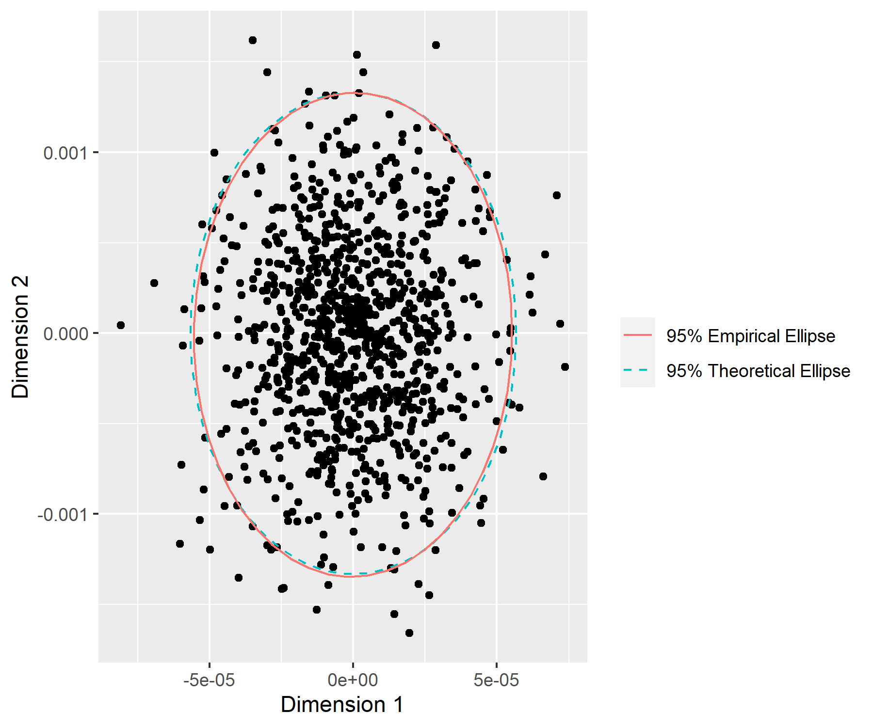
Figure 2: Plot of 1000 Monte Carlo iterations of the first row of $\widehat{U}\mathcal{O}_{*}-U$ with the same $M$ matrix as above and $n=d=1800$ with $n_{1}=n_{2}=n_{3}=600$. The covariances here are spherical within each mixture component, though they differ between components. The dotted line represents the theoretical 95 percent confidence ellipse from Theorem 1 and Corollary 2. The solid line is the estimated ellipse. The different scalings on the two axes arise because the variances in these two dimensions are proportional to the first two squared singular values of $M$, as seen in Corollary 1. Further details are in Section 4.

4.1 Elliptical Versus Spherical Covariances

In Figure 3 we examine the effect of elliptical covariances on the limiting distribution predicted by Corollary 2. We consider the same $M$ matrix and mixture sizes as in Figure 1, only we fix the covariances as

$$\Sigma_{E}^{(1)}: =F_{1}F_{1}^{\top}+.1I_{d}$$

$$\Sigma^{(2)}: =F_{2}F_{2}^{\top}+I_{d}$$

$$\Sigma^{(3)}: =2I_{d},$$

where $F_{1}$ and $F_{2}$ are square matrices with entries drawn independently from uniform distributions on $[0,.003]$ and $[0,.001]$ respectively. We also consider the spherical case $\Sigma_{S}^{(1)}=VV^{\top}+I_{d}$. We run 1000 iterations of this simulation and examine the first row of the matrix $(\widehat{U}\mathcal{O}_{*}-U)\Lambda$, where again $\mathcal{O}_{*}$ is estimated using the procrustes difference between $\widehat{U}$ and $U$. The only thing we change between each dataset is the covariance; i.e., we draw $E_{1}\in\mathbb{R}^{n_{1}\times d}$ as a random Gaussian matrix with independent entries and multiply by $(\Sigma_{E}^{(1)})^{1/2}$ or $(\Sigma_{S}^{(1)})^{1/2}$ to obtain the first $n_{1}$ rows of the matrix $E$. We keep the other $n-n_{1}$ rows fixed within each Monte Carlo iteration, so the only randomness for each iteration is in drawing the $nd$ Gaussian random variables.

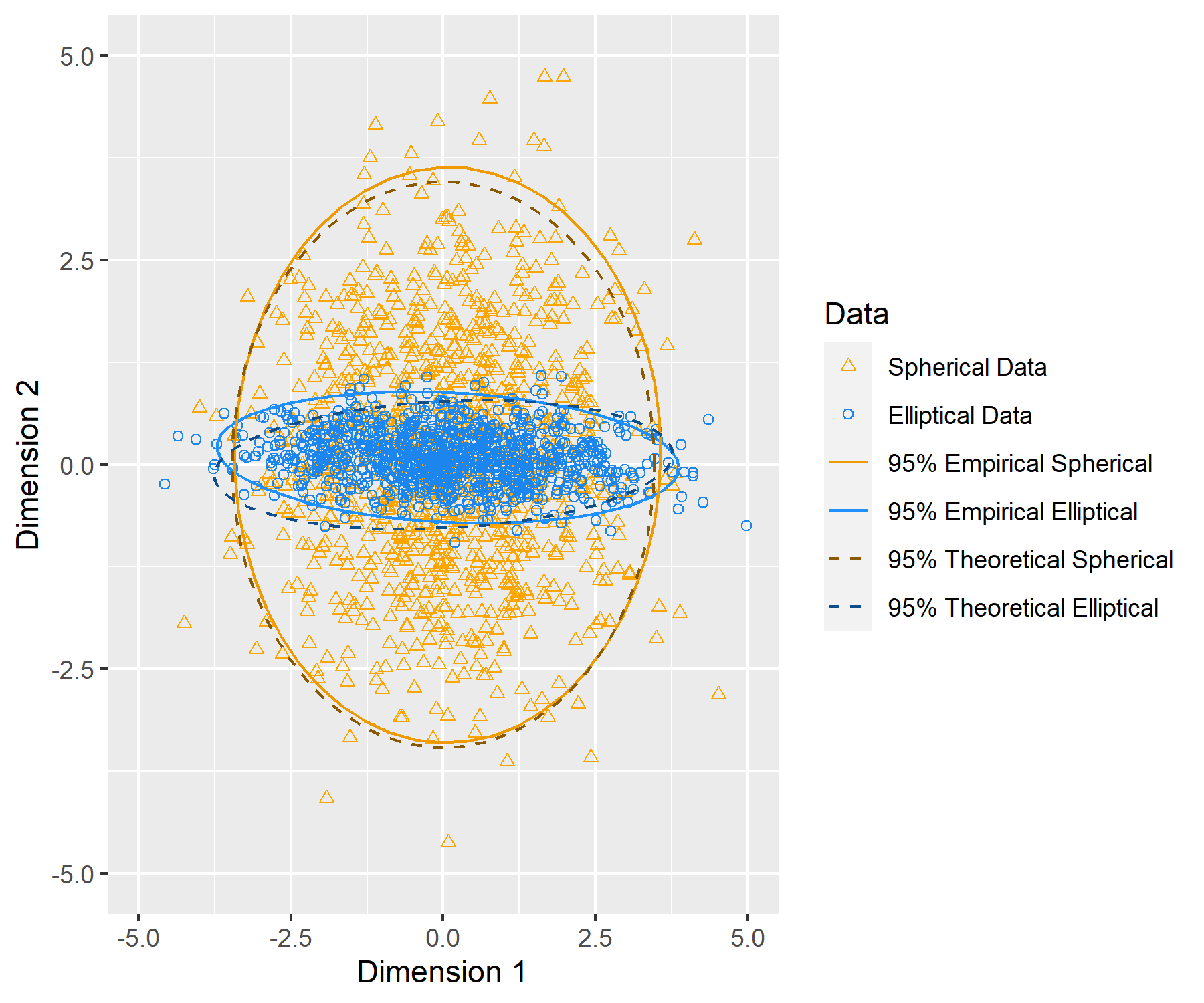
Figure 3: Comparison of $\Lambda(\widehat{U}\mathcal{O}_{*}-U)_{1\cdot}$ for the same mixture distribution as above, only we modify the covariance for the first mixture component between each data set. Details are in Section 4.1.

We scale $\widehat{U}\mathcal{O}_{*}-U$ by $\Lambda$ in order to explicitly showcase the covariance structure. The way we create $\Sigma_{E}^{(1)}$ yields that the limiting covariance $S_{E}^{(1)}$ is approximately

$$S_{E}^{(1)}:=\Lambda^{-1}\begin{pmatrix}2.35&0.083\\ 0.083&0.104\end{pmatrix}\Lambda^{-1},$$

so that $\Lambda(\widehat{U}\mathcal{O}_{*}-U)_{1\cdot}$ is approximately Gaussian with covariance $\begin{pmatrix}2.35&0.083\\ 0.083&0.104\end{pmatrix}$. On the other hand, when we consider the spherical case, we see that $S_{S}^{(1)}$ is of the form

$$S_{S}^{(1)} =2\Lambda^{-2}$$

so that $\Lambda(\widehat{U}\mathcal{O}_{*}-U)_{1\cdot}$ is approximately Gaussian with covariance $2I_{r}$. Figure 3 shows these differences, where we plot the empirical 95% confidence ellipses with respect to both the estimated covariance (solid line) and theoretical covariance (dashed line).

To study the relationship between $\Sigma_{i}$ and $V$ in more detail, we also consider the following setting. We consider the class-wise covariances again

$$\Sigma^{(1)}: =15F_{1}F_{1}^{\top}+.1I_{d}$$

$$\Sigma_{\theta}^{(2)}: =5V_{\cdot 1}V_{\cdot 1}^{\top}+5V_{2}^{\theta}(V_{2}^{\theta})^{\top}+.1I_{d}$$

$$\Sigma^{(3)}: =10F_{3}F_{3}^{\top}+.1I_{d},$$

where again $F_{1}$ and $F_{3}$ are drawn uniformly from the Stiefel manifold of dimension 100 and 200 respectively, with $n_{1}=200$ and $n_{2}=n_{3}=400$. We also change $\mu_{3}=(5,\ldots,5,6,\ldots 6)$ to better separate the clusters. The vector $V_{2}^{\theta}$ is orthogonal to $V_{\cdot 1}$ and satisfies $\langle V_{2}^{\theta},V_{\cdot 2}\rangle=\theta$ for $\theta\in\{.9,.5,.1\}$. As $\theta$ decreases, the limiting covariance matrix in Corollary 2 will change along the second dimension only. Figure 4 reflects this theory, where we plot 1000 Monte Carlo runs of $\Lambda(\widehat{U}\mathcal{O}_{*}-U)_{(n_{1}+1)\cdot}$. The variance stays fixed along the first dimension, but it shrinks along the second dimension, showcasing the geometric relationship between $V$ and $\Sigma^{(2)}$ as suggested by Corollary 2.

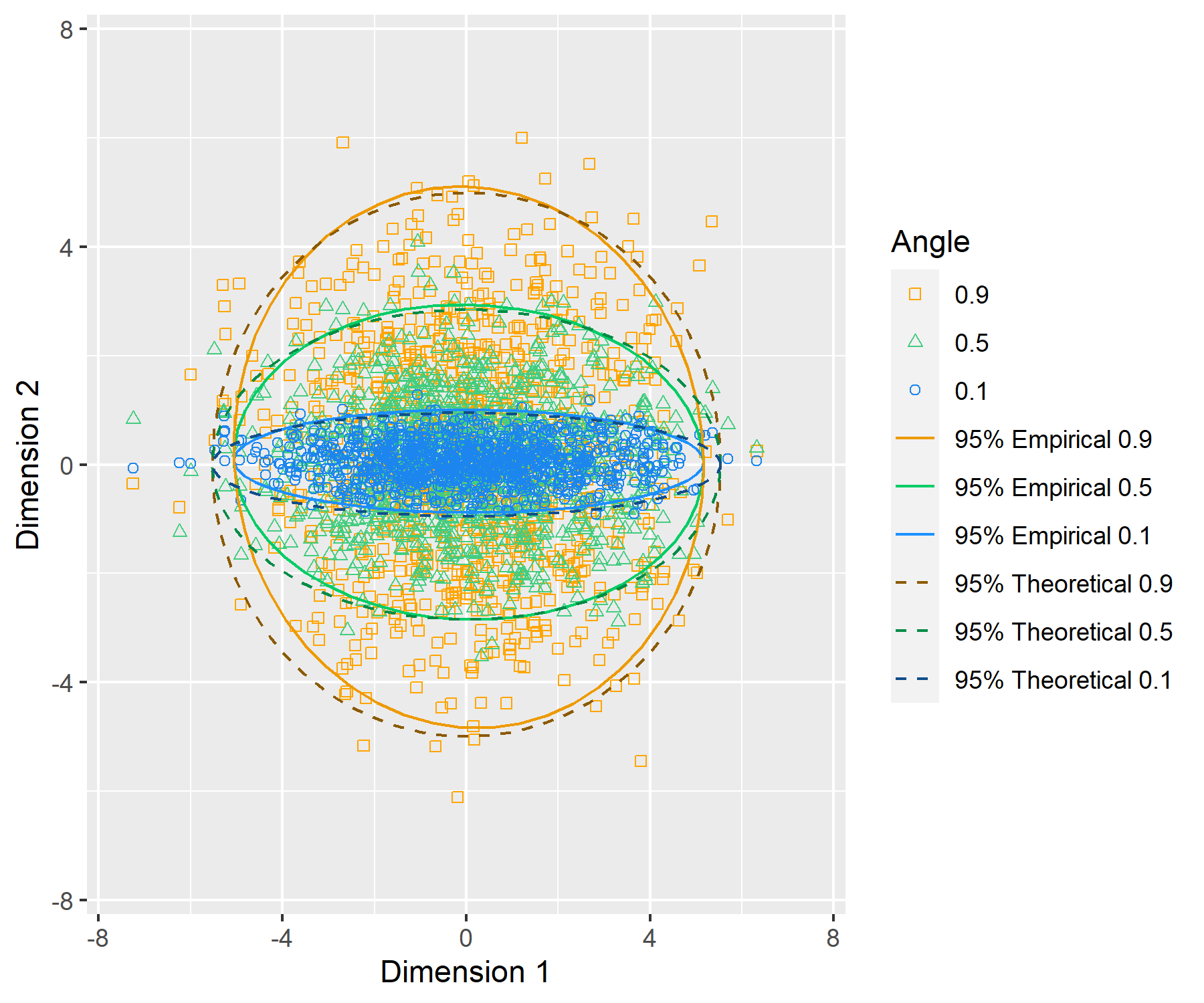
Figure 4: Comparison of $\Lambda(\widehat{U}\mathcal{O}_{*}-U)_{(n_{1}+1)\cdot}$ for the same mixture distribution as above, only we modify the covariance for the second mixture component between each data set by changing the angle between the leading covariance and the second mixture component. Details are in Section 4.1.

5 Discussion

We have shown that under general model assumptions for the noise matrix, allowing for heteroskedasticity between rows and dependence within them, that the entries of the left singular vectors of the output from HeteroPCA are consistent estimators for those of the original signal matrix $M$, and the errors are asymptotically normally-distributed in a natural high-dimensional regime. Furthermore, our Berry-Esseen theorem makes clear the rate at which this asymptotic approximation becomes valid, revealing the effect of the relationship between the noise covariances and the spectral structure of the signal matrix on the distributional convergence. In the particular case that the individual covariances are scalar multiples of the identity, our results also show that the variances of the entries of the $j$’th estimated singular vector are proportional to the inverse $j$’th singular value of the signal matrix. In particular, this means that estimating additional singular vectors in this model becomes more challenging and requires more data, since the variance in this estimation grows with $j$.

In this paper, we assume the rank $r$ is known a priori, but in practice one may need to estimate $r$ using, for example, the methods proposed in Zhu and Ghodsi (2006), Han et al. (2020), or Yang et al. (2020). In addition, while our results highlight the interplay of the dependence structure of the noise with the signal matrix, additional work is required to make the upper bound computable from observed data. For example, our results do not imply consistent estimation for the row-wise covariance matrices $\Sigma_{i}$, though we do show if one has covariances that are only distinct between clusters, then one can estimate the limiting covariance matrix $S_{i}$ for each row of $\widehat{U}$. Our techniques could therefore be appropriately modified to develop two-sample asymptotically valid confidence regions or test statistics, such as in deriving a Hotelling $T^{2}$ analogue for the singular vectors as in Fan et al. (2019); Du and Tang (2021). Furthermore, one possibility for further inference would be to consider drawing several matrices $M+E$ independently from the same distribution, assuming the rows are matched together between samples, in which case one could leverage existing statistical methodology to conduct two-sample tests of hypothesis.

Another possible extension is estimating linear forms of singular vectors under the dependence structure we consider, which has been studied in other settings under independent noise. Our results naturally extend to sufficiently sparse linear forms (i.e. linear forms $T$ such that $\|TU\|\leq b\|U\|_{2,\infty}$), but studying linear forms for which $\|TU\|\asymp 1$ would require additional methods, as the entrywise analysis methods we use would not be applicable. Finally, our results hold for a natural subgaussian mixture model, but many high-dimensional datasets contain outlier vectors or heavier tails, in which case additional techniques are required.

6 Proof Architecture for Theorems 1 and 2

In this section we state several intermediate lemmas, prove Theorem 2, and sketch the proof of Theorem 1. Full proofs are in the appendices. First we collect some initial spectral norm bounds that are useful in the sequel. The first is a bound on the noise error $\|\Gamma(Z)\|$, the proof of which is adapted from Theorem 2 in Amini and Razaee (2021). Throughout this section and all the proofs, we allow constants $C$ to change from line to line.

Lemma 1 (Spectral Norm Concentration).

Under assumption 1, there exists a universal constant $C_{\text{spectral}}$ such that with probability at least $1-4(n\vee d)^{-6}$

$$\|\Gamma(EM^{\top}+ME^{\top}+EE^{\top})\|\leq C_{\text{spectral}}\bigg{(}\sigma^{2}(n+\sqrt{nd})+\sigma\sqrt{n}\kappa\lambda_{r}\bigg{)}.$$

The next bound shows that the approximation of $\tilde{A}=A+\Gamma(Z)$ to $\widehat{A}$, the output of the HeteroPCA algorithm, is much smaller than the approximation of $\tilde{A}$ to $A$. Recall that $N_{T}$ denotes the approximation of $A$ from Algorithm 1 after $T$ iterations. We note that the existence of $T_{0}$ in the statement of this lemma follows from Zhang et al. (2021) and Assumptions 3 and 4.In particular, if we take $T_{0}\geq C\log\left(\frac{\lambda_{r}^{2}}{\|\Gamma(Z)\|}\right)$, then by the proof of Theorem 7 in Zhang et al. (2021), it holds that $\|N_{T}-A\|\leq 3\|\Gamma(Z)\|$.

Lemma 2.

Define $T_{0}$ as the first iteration such that $\|N_{T}-A\|\leq 3\|\Gamma(Z)\|$. Let $\rho=10\|\Gamma(Z)\|/\lambda_{r}^{2}$, and suppose Assumption 2.Define $\tilde{K}_{T}:=\|N_{T}-\tilde{A}\|$. Then for all $T\geq T_{0}$ and $n$ large enough, on the event in Lemma 1, we have that $\rho<\frac{1}{2}$, and

$$\tilde{K}_{T} \leq 4\rho^{T-T_{0}}\|\Gamma(Z)\|+\frac{20}{1-\rho}\|U\|_{2,\infty}\|\Gamma(Z)\|.$$

Consequently, when $T=\Theta\left(\log\left(\frac{\lambda_{r}^{2}}{\|U\|_{2,\infty}\|\Gamma(Z)\|}\right)\right)$, it holds that

$$\|\widehat{A}-\tilde{A}\|\leq 41\|U\|_{2,\infty}\|\Gamma(Z)\|.$$

Assumption 2 implies that

$$\lambda_{r}^{2} \geq C\bigg{(}\sigma^{2}rd\log(n\vee d)+\sigma\sqrt{nr\log(n\vee d)}\kappa\lambda_{r}\bigg{)},$$

which ensures that that there is an eigengap on the event in Lemma 1. Therefore, a standard application of the Davis-Kahan Theorem (e.g. Chen et al. (2021b)) and Lemma 1 immediately implies that $\widehat{U}\widehat{U}^{\top}-UU^{\top}$ tends to zero in spectral norm.

To prove our main $\ell_{2,\infty}$ result, we analyze the statistical error and algorithmic error separately. Define $H:=U^{\top}\tilde{U}$, and $\tilde{H}:=\tilde{U}^{\top}\widehat{U}$. First, write $\widehat{U}-U\mathcal{O}$ as

$$\widehat{U}-U\mathcal{O}=(\widehat{U}-\tilde{U}\tilde{H})+(\tilde{U}-UH)\tilde{H}+U(H\tilde{H}-\mathcal{O}).$$

The first term captures the algorithmic error between the eigenvectors of the output of Algorithm 1, $\widehat{A}$, and those of the matrix it approximates, $\tilde{A}$. The next term is the statistical error between the matrix $\tilde{A}$ approximated by the algorithm and the true matrix of interest $A$. Finally, we have a correction term which accounts for the fact that $\tilde{H}$ and $H$ are contractions rather than orthogonal matrices.

Since the bound on the algorithmic error depends on the properties of $\tilde{U}$, we first prove the bound on the middle term, or the statistical error between $\tilde{U}$ and $U$. Then we bound the algorithmic error and finally the correction term. The following result bounds the statistical error between $\tilde{U}$ and $UH$ with high probability.

Theorem 3.

Under Assumptions 1, 2, 3 and 4, we have that there exists a universal constant $C_{R}$ such that

$$\|\tilde{U}-UH\|_{2,\infty} \leq C_{R}\bigg{(}\frac{\sqrt{rnd}\log(\max(n,d))\sigma^{2}}{\lambda_{r}^{2}}+\frac{\sqrt{rn\log(n\vee d)}\kappa\sigma}{\lambda_{r}}\bigg{)}\|U\|_{2,\infty}$$

with probability at least $1-(n\vee d)^{-4}$.

In order to prove this result, we use the matrix series expansion developed in Xia (2019b) to write the difference of projection matrices in terms of the noise matrix, each term of which requires careful considerations due to the dependence between columns of the noise matrix $E$.

Consequently, by Assumption 2, the result in Theorem 3 implies that

$$\|\tilde{U}\|_{2,\infty} \leq\|\tilde{U}-UH\|_{2,\infty}+\|U\|_{2,\infty}$$

$$\lesssim\|U\|_{2,\infty},$$

which shows that the matrix $\tilde{U}$ is just as incoherent as $U$ up to constant factors. We also have the following result for the deterministic analysis.

Theorem 4.

Define $\tilde{H}:=\tilde{U}^{\top}\widehat{U}$. Suppose the event in Theorem 3 holds. Then, in the setting of Lemma 2, we have that there exists a universal constant $C_{D}$ such that

$$\|\widehat{U}-\tilde{U}\tilde{H}\|_{2,\infty}\leq C_{D}\kappa^{2}\frac{\|U\|_{2,\infty}^{2}\|\Gamma(Z)\|}{\lambda_{r}^{2}}.$$

Finally, we consider the correction term.

Lemma 3.

There exists an orthogonal matrix $\mathcal{O}_{*}$ and a universal constant $C$ such that under Assumptions 2 and 4, the event in Lemma 1, and $T=\Theta\left(\frac{\lambda_{r}^{2}}{\|U\|_{2,\infty}\|\gamma(Z)\|}\right)$,

$$\|UH\tilde{H}-U\mathcal{O}_{*}^{\top}\|_{2,\infty} \leq C\|U\|_{2,\infty}\frac{\|\Gamma(Z)\|^{2}}{\lambda_{r}^{4}}.$$

We now have all the pieces to prove Theorem 2.

Proof of Theorem 2.

We note that all the events that determine Lemmas 2, 3, and Theorem 4 are the event in Lemma 1, and the event in Theorem 3. Taking a union bound, these events occur simultaneously with probability at least $1-(n\vee d)^{-4}-4(n\vee d)^{-6}\geq 1-2(n\vee d)^{-4};$ henceforth we operate on the intersection of these events. Since Theorem 3 gives the stated upper bound for $\|\tilde{U}-UH\|_{2,\infty}$ on this set, by increasing the constants if necessary, we need only show that this bound holds for the algorithmic error $\|\widehat{U}-\tilde{U}\tilde{H}\|_{2,\infty}$, and the correction term $\|UH\tilde{H}-U\mathcal{O}_{*}\|_{2,\infty}$.

Under assumption 4, we have that

$$\kappa^{2}\|U\|_{2,\infty} \leq\kappa^{2}\mu_{0}\sqrt{r/n}$$

$$\leq\sqrt{r\log(n\vee d)}.$$

Hence, the bound in Theorem 4 becomes

$$\|\widehat{U}-\tilde{U}\widehat{H}\|_{2,\infty}\leq C_{D}\|U\|_{2,\infty}\sqrt{r\log(n\vee d)}\frac{\|\Gamma(Z)\|}{\lambda_{r}^{2}}.$$ (2)

In addition, on the event of Lemma 1,

$$\|\Gamma(Z)\|\leq C_{\text{spectral}}\bigg{(}\sigma^{2}(n+\sqrt{nd})+\sigma\sqrt{n}\kappa\lambda_{r}\bigg{)}.$$

This gives the desired bound for the algorithmic error. For the correction term, we note that the upper bound in Lemma 3 does not exceed that of Equation (2), which has already been bounded.

Combining these bounds, there is a constant $C>0$ such that with probability at least $1-2(n\vee d)^{-4}$,

$$\inf_{\mathcal{O}\in\mathbb{O}(r)}\|\widehat{U}-U\mathcal{O}\|_{2,\infty}\leq C\bigg{(}\frac{\sqrt{rnd}\log(n\vee d)\sigma^{2}}{\lambda_{r}^{2}}+\frac{\sqrt{rn\log(n\vee d)}\kappa\sigma}{\lambda_{r}}\bigg{)}\|U\|_{2,\infty},$$

as advertised. ∎

In order to prove Theorem 1, we show that

$$e_{i}^{\top}\left(\widehat{U}\mathcal{O}_{*}-U\right)e_{j} =\langle E_{i},V_{\cdot j}\rangle\lambda_{j}^{-1}+R,$$ (3)

where $V_{\cdot j}$ is the $j$’th column of $V$ and $R$ is a residual term that we bound using similar ideas to the proof of Theorem 2. A straightforward calculation reveals that $\mathbb{E}\bigg{(}\langle E_{i},V_{\cdot j}\rangle\lambda_{j}^{-1}\bigg{)}^{2}=V_{\cdot j}^{\top}\Sigma_{i}V_{\cdot j}\lambda_{j}^{-2}$, and hence if we define $\sigma_{ij}:=\|\Sigma_{i}^{1/2}V_{\cdot j}\|\lambda_{j}^{-1}$, we have that

$$\frac{\langle E_{i},V_{\cdot j}\rangle\lambda_{j}^{-1}}{\sigma_{ij}} =\frac{\langle E_{i},V_{\cdot j}\rangle}{\|\Sigma_{i}^{1/2}V_{\cdot j}\|}$$

$$=\frac{\langle Y_{i},\Sigma_{i}^{1/2}V_{\cdot j}\rangle}{\|\Sigma_{i}^{1/2}V_{\cdot j}\|},$$

which by Assumption 1 is a sum of $d$ independent mean-zero random variables to which the classical Berry-Esseen Theorem (Berry, 1941) can be applied. The residual term $R$ consists of higher-order terms stemming from a matrix series expansion (see Lemma 5 in Appendix A). However, we have already bounded many of these residual terms as part of the proof of Theorem 3, so we need only show that dividing the residual terms by $\sigma_{ij}$ yields convergence to zero. We then use the Lipschitz property of the Gaussian cumulative distribution function to complete the proof of the theorem.

Appendix A Proof of Theorem 3

First, note that it holds that

$$\|\tilde{U}\widehat{H}-U\tilde{H}\widehat{H}\|_{2,\infty} \leq\|\tilde{U}-U\tilde{H}\|_{2,\infty}$$

$$\leq\|\tilde{U}\tilde{U}^{\top}-UU^{\top}\tilde{U}\tilde{U}^{\top}\|_{2,\infty}$$

$$\leq\|\tilde{U}\tilde{U}^{\top}-UU^{\top}\|_{2.\infty}\|\tilde{U}\tilde{U}^{\top}\|$$

$$\leq\|\tilde{U}\tilde{U}^{\top}-UU^{\top}\|_{2,\infty},$$

which is a difference of projection matrices. We now wish to expand $\tilde{U}\tilde{U}^{\top}$ in terms of the noise matrix $\Gamma(EM^{\top}+ME^{\top}+EE^{\top})$.

In what follows, define, for some sufficiently large constant $C_{0}$

$$\delta_{1}: =\sqrt{rnd}\log(\max(n,d))\sigma^{2};$$

$$\delta_{2}: =\sqrt{rn\log(n\vee d)}\lambda_{1}\sigma;$$

$$\delta: =C_{0}(\delta_{1}+\delta_{2}).$$

The two terms $\delta_{1}$ and $\delta_{2}$ appear frequently in our bounds, so this notation simplifies the statements of several of our results. With this new notation, to prove Theorem 3 it is sufficient to show that

$$\|\tilde{U}\tilde{U}^{\top}-UU^{\top}\|_{2,\infty} \leq C_{R}\frac{\delta}{\lambda_{r}^{2}}\|U\|_{2,\infty}.$$

It is slightly more mathematically convenient to study the perturbation $EM^{\top}+ME^{\top}+\Gamma(EE^{\top})$, so we introduce the matrix $\tilde{U}_{D}\tilde{U}_{D}^{\top}$ which is the projection onto the leading eigenspace of the matrix $MM^{\top}+ME^{\top}+EM^{\top}+\Gamma(EE^{\top})$. We have the following spectral norm guarantee that shows that $\tilde{U}_{D}\tilde{U}_{D}^{\top}$ and $\tilde{U}\tilde{U}^{\top}$ are exceedingly close.

Lemma 4.

With probability at least $1-2(n\vee d)^{-5}$,

$$\|\tilde{U}_{D}\tilde{U}_{D}^{\top}-\tilde{U}\tilde{U}^{\top}\|\leq\frac{C\delta_{1}}{\lambda_{r}^{2}}\|U\|_{2,\infty}$$

By Lemma 1 and Lemma 4, we have that with probability at least $1-c(n\vee d)^{-5}$ that

$$\|EM^{\top}+ME^{\top}+\Gamma(EE^{\top})\| \leq\frac{\delta}{\sqrt{r\log(n\vee d)}}$$

provided $C_{0}$ is sufficiently large.

In order to analyze the approximation of $\tilde{U}_{D}\tilde{U}_{D}^{\top}$ to $UU^{\top}$, we will use the projection matrix expansion in Xia (2019a), restated slightly for our purposes here.

Lemma 5 (Theorem 1 from Xia (2019b)).

Let $U$ be the eigenvectors of $A$ corresponding to its nonzero eigenvalues and let $\tilde{U}_{D}$ be the eigenvectors of $A+W$, where $\|W\|\leq\frac{\lambda_{r}^{2}}{2}$. Then $\tilde{U}_{D}$ admits the series expansion

$$\tilde{U}_{D}\tilde{U}_{D}^{\top} =UU^{\top}+\sum_{p\geq 1}S_{A,k}(W),$$

where $S_{A,p}$ is defined according to Xia (2019b) via

$$S_{A,p}(W) =\sum_{\mathbf{s}:s_{1}+\cdots+s_{p+1}=p}(-1)^{1+\tau(\mathbf{s})}\mathcal{P}^{-s_{1}}W\mathcal{P}^{-s_{2}}W\cdots W\mathcal{P}^{-s_{p+1}},$$

where $\mathcal{P}^{-p}=U\Lambda^{-2p}U^{\top}$, and $\mathcal{P}^{0}=U_{\perp}U_{\perp}^{\top}$.

By Assumption 2, we have that $\lambda_{r}^{2}\geq 2\|EM^{\top}+ME^{\top}+\Gamma(EE^{\top})\|$, and hence the assumptions to apply the expansion in Lemma 5 hold. Let $W:=ME^{\top}+EM^{\top}+\Gamma(EE^{\top})$. We note that we therefore have

$$\tilde{U}_{D}\tilde{U}_{D}^{\top}-UU^{\top} =\sum_{p\geq 1}S_{MM^{\top},p}(W),$$

Note that if $s_{1}\geq 1$, $\|U\Lambda^{-2s_{1}}U^{\top}W\cdots U\Lambda^{-2s_{p+1}}U^{\top}\|_{2,\infty}\leq\|U\|_{2,\infty}\lambda_{r}^{-2p}\|W\|^{p}$ which is bounded above by $\delta^{p}\lambda_{r}^{-2p}\|U\|_{2,\infty}$ by Lemma 1. Hence, it suffices to bound terms of the form

$$\|(U_{\perp}U_{\perp}^{\top}WU_{\perp}U_{\perp}^{\top})^{p}WU\|_{2,\infty}.$$

We have the following lemma characterizing terms of this form, whose proof is in Appendix E. This proof requires additional considerations about dependence which requires specially crafted “leave-one-out" terms that have hitherto not been considered in the literature on entrywise eigenvector analysis.

Lemma 6.

Let $W=EM^{\top}+ME^{\top}+\Gamma(EE^{\top})$. There exists universal constants $C_{1}$ and $C_{2}$ such that for any $p\geq 1$, we have that with probability at least $1-(p+1)(n\vee d)^{-5}$ for all $1\leq p_{0}\leq p$ that

$$\|(U_{\perp}U_{\perp}^{\top}WU_{\perp}U_{\perp}^{\top})^{p_{0}-1}WU\|_{2,\infty}\leq C_{1}(C_{2}\delta)^{p_{0}}\|U\|_{2,\infty},$$

Let $c$ be some number to be chosen later. There are at most $4^{p}$ terms such that $s_{1}+\cdots+s_{p+1}=p$, and hence

$$\|\sum_{p\geq 1}S_{A,k}(W)\|_{2,\infty} \leq\sum_{p=1}^{c\log(n\vee d)}\|S_{A,p}(W)\|_{2,\infty}+\sum_{p=c\log(n\vee d)}^{\infty}\|S_{A,p}(W)\|_{2,\infty}$$

$$\leq\|U\|_{2,\infty}\sum_{p=1}^{c\log(n\vee d)}C_{1}\bigg{(}\frac{4C_{2}\delta}{\lambda_{r}^{2}}\bigg{)}^{p}+\sum_{p=c\log(n\vee d)}^{\infty}\bigg{(}\frac{4\|W\|}{\lambda_{r}^{2}}\bigg{)}^{p}$$

$$\leq C\|U\|_{2,\infty}\frac{\delta}{\lambda_{r}^{2}}+\frac{1}{2^{c\log(n\vee d)}}$$

$$\leq C_{R}\|U\|_{2,\infty}\frac{\delta}{\lambda_{r}^{2}},$$

where in the final line we have used the fact that the second term can be bounded by $2^{-c\log(n\vee d)}\leq\|U\|_{2,\infty}$ for $c$ taken to be sufficiently large. Finally, this bound holds with probability at least $1-c\log(n\vee d)(n\vee d)^{-5}-4(n\vee d)^{-6}\geq 1-(n\vee d)^{-4}$, which completes the proof of Theorem 3.

Appendix B Proof of Theorem 4

First, we have the following result on the eigengap.

Lemma 7.

Suppose Assumption 2 holds, and suppose $T\geq T_{0}$, where $T_{0}$ is the first iterate such that $\|N_{T}-A\|\leq 3\|\Gamma(Z)\|$. Then on the event in Lemma 1, we have

$$(\widehat{\lambda}_{r}^{(T)})^{2}-\tilde{\lambda}_{r+1}^{2}\geq\lambda_{r}^{2}/2.$$

In particular,

$$\widehat{\lambda}_{r}^{2}-\tilde{\lambda}_{r+1}^{2}\geq\lambda_{r}^{2}/2.$$

Proof.

$\widehat{\lambda}_{r}^{2}\geq\tilde{\lambda}_{r}^{2}-\|N_{T}-\tilde{A}\|\geq\tilde{\lambda}_{r}^{2}-4\|\Gamma(Z)\|$ once $T\geq T_{0}$. Then $\widehat{\lambda}_{r}^{2}-\tilde{\lambda}_{r+1}^{2}\geq\tilde{\lambda}_{r}^{2}-\tilde{\lambda}_{r+1}^{2}-4\|\Gamma(Z)\|\geq\lambda_{r}^{2}-\lambda_{r+1}^{2}-6\|\Gamma(Z)\|=\lambda_{r}^{2}-6\|\Gamma(Z)\|$. On the event in Lemma 1, $\|\Gamma(Z)\|\leq C_{\mathrm{spectral}}(\sigma^{2}(n+\sqrt{nd})+\sigma\sqrt{n}\kappa\lambda_{r}),$ and under the signal-to-noise ratio condition of Assumption 2,

$$\lambda_{r}^{2}\geq 12C_{\mathrm{spectral}}\left(\sigma^{2}(n+\sqrt{nd})+\sigma\sqrt{n}\kappa\lambda_{r}\right),$$

this gives

$$\|\Gamma(Z)\|\leq\frac{1}{12}\lambda_{r}^{2},$$

meaning that

$$\widehat{\lambda}_{r}^{2}-\tilde{\lambda}_{r+1}^{2}\geq\lambda_{r}^{2}/2.$$

∎

We can now prove Theorem 4.

Proof of Theorem 4.

We write:

$$\widehat{U}-\tilde{U}\tilde{U}^{\top}\widehat{U} =P_{\tilde{U}}\tilde{A}[\widehat{U}-\tilde{U}\tilde{H}]\widehat{\Lambda}^{-1}+[N_{T}-P_{\tilde{U}}\tilde{A}][\widehat{U}-\tilde{U}\tilde{H}]\widehat{\Lambda}^{-1}$$

$$\qquad+[N_{T}-P_{\tilde{U}}\tilde{A}]\tilde{U}\tilde{H}\widehat{\Lambda}^{-1}-\tilde{U}[\tilde{H}\widehat{\Lambda}-\tilde{\Lambda}\tilde{H}]\widehat{\Lambda}^{-1}$$

$$: =J_{1}+J_{2}+J_{3}+J_{4}.$$

We bound each term successively.

The term $J_{1}$: Note that $\|\widehat{U}-\tilde{U}\tilde{H}\|\leq\sqrt{2}\|\sin\Theta(\widehat{U},\tilde{U})\|.$ Therefore, we have that

$$\|P_{\tilde{U}}\tilde{A}[\widehat{U}-\tilde{U}\tilde{H}]\widehat{\Lambda}^{-1}\|_{2,\infty} \leq\|P_{\tilde{U}}\tilde{A}\|_{2,\infty}\|\widehat{U}-\tilde{U}\tilde{H}\|\|\widehat{\Lambda}^{-1}\|$$

$$\leq\|\tilde{U}\tilde{\Lambda}\tilde{U}\|_{2,\infty}\|\widehat{U}-\tilde{U}\tilde{H}\|\widehat{\lambda}_{r}^{-2}$$

$$\leq\frac{\tilde{\lambda}_{1}^{2}}{\widehat{\lambda}_{r}^{2}}\|\tilde{U}\|_{2,\infty}\|\widehat{U}-\tilde{U}\tilde{H}\|$$

$$\leq\sqrt{2}\frac{\tilde{\lambda}_{1}^{2}}{\widehat{\lambda}_{r}^{2}}\|\tilde{U}\|_{2,\infty}\|\sin\Theta(\widehat{U},\tilde{U})\|.$$ (4)

The term $J_{2}$: We decompose via

$$[N_{T}-P_{\tilde{U}}\tilde{A}][\widehat{U}-\tilde{U}\tilde{H}]\widehat{\Lambda}^{-1} =\widehat{U}[\widehat{\Lambda}\widehat{U}^{\top}-\tilde{H}^{\top}\tilde{\Lambda}\tilde{U}^{\top}][\widehat{U}-\tilde{U}\tilde{H}]\widehat{\Lambda}^{-1}+[\widehat{U}-\tilde{U}\tilde{H}]\tilde{H}^{\top}\tilde{\Lambda}\tilde{U}^{\top}[\widehat{U}-\tilde{U}\tilde{H}]\widehat{\Lambda}^{-1}$$

$$\quad-\tilde{U}[I-\tilde{H}\tilde{H}^{\top}]\tilde{\Lambda}\tilde{U}^{\top}[\widehat{U}-\tilde{U}\tilde{H}]\widehat{\Lambda}^{-1}.$$

Note that $\tilde{U}^{\top}[\widehat{U}-\tilde{U}\tilde{H}]=0$, by the definition of $\tilde{H}$, whence we have

$$[N_{T}-P_{\tilde{U}}\tilde{A}][\widehat{U}-\tilde{U}\tilde{H}]\widehat{\Lambda}^{-1} =\tilde{U}\tilde{H}[\widehat{\Lambda}\widehat{U}^{\top}-\tilde{H}^{\top}\tilde{\Lambda}\tilde{U}^{\top}][\widehat{U}-\tilde{U}\tilde{H}]\widehat{\Lambda}^{-1}+[\widehat{U}-\tilde{U}\tilde{H}][\widehat{\Lambda}\widehat{U}^{\top}-\tilde{H}^{\top}\tilde{\Lambda}\tilde{U}^{\top}][\widehat{U}-\tilde{U}\tilde{H}]\widehat{\Lambda}^{-1}$$

$$=\tilde{U}\tilde{H}\widehat{\Lambda}[\widehat{U}-\tilde{U}\tilde{H}]^{\top}[\widehat{U}-\tilde{U}\tilde{H}]\widehat{\Lambda}^{-1}+[\widehat{U}-\tilde{U}\tilde{H}]\widehat{\Lambda}[I-\tilde{H}^{\top}\tilde{H}]\widehat{\Lambda}^{-1}.$$

Taking norms, we have

$$\|[N_{T}-P_{\tilde{U}}\tilde{A}][\widehat{U}-\tilde{U}\tilde{H}]\widehat{\Lambda}^{-1}\|_{2,\infty}\leq\|\tilde{U}\|_{2,\infty}\widehat{\lambda}_{1}^{2}\|\widehat{U}-\tilde{U}\tilde{H}\|^{2}\widehat{\lambda}_{r}^{-2}+\|\widehat{U}-\tilde{U}\tilde{H}\|_{2,\infty}\widehat{\lambda}_{1}^{2}\|I-\tilde{H}^{\top}\tilde{H}\|\widehat{\lambda}_{r}^{-2}$$

Recall that $\|I-\tilde{H}^{\top}\tilde{H}\|\leq\|\widehat{U}\widehat{U}^{\top}-\tilde{U}\tilde{U}^{\top}\|\leq 2\|\sin\Theta(\widehat{U},\tilde{U})\|$, and $\|\widehat{U}-\tilde{U}\tilde{H}\|\leq\sqrt{2}\|\sin\Theta(\widehat{U},\tilde{U})\|.$ Consequently,

$$\|J_{2}\|_{2,\infty} \leq 2\|\tilde{U}\|_{2,\infty}\frac{\widehat{\lambda}_{1}^{2}}{\widehat{\lambda}_{r}^{2}}\|\sin\Theta(\widehat{U},\tilde{U})\|^{2}+2\|\widehat{U}-\tilde{U}\tilde{H}\|_{2,\infty}\frac{\widehat{\lambda}_{1}^{2}}{\widehat{\lambda}_{r}^{2}}\|\sin\Theta(\widehat{U},\tilde{U}\|.$$ (5)

The term $J_{3}$: Again using the fact that $\tilde{U}^{\top}[\widehat{U}-\tilde{U}\tilde{H}]=0$,

$$[N_{T}-P_{\tilde{U}}\tilde{A}][\widehat{U}-\tilde{U}\tilde{H}]\widehat{\Lambda}^{-1} =\widehat{U}\widehat{\Lambda}[I-\tilde{H}^{\top}\tilde{H}]\widehat{\Lambda}^{-1}$$

$$=\tilde{U}\tilde{H}\widehat{\Lambda}[I-\tilde{H}^{\top}\tilde{H}]\widehat{\Lambda}^{-1}+[\widehat{U}-\tilde{U}\tilde{H}]\widehat{\Lambda}[I-\tilde{H}^{\top}\tilde{H}]\widehat{\Lambda}^{-1}.$$

This gives

$$\|[N_{T}-P_{\tilde{U}}\tilde{A}][\widehat{U}-\tilde{U}\tilde{H}]\widehat{\Lambda}^{-1}\|_{2,\infty} \leq\|\tilde{U}\|_{2,\infty}\widehat{\lambda}_{1}^{2}\|I-\tilde{H}^{\top}\tilde{H}\|\widehat{\lambda}_{r}^{-2}+\|\widehat{U}-\tilde{U}\tilde{H}\|_{2,\infty}\widehat{\lambda}_{1}^{2}\|I-\tilde{H}^{\top}\tilde{H}\|\widehat{\lambda}_{r}^{-2}$$

$$\leq 2(\|\tilde{U}\|_{2,\infty}+\|\widehat{U}-\tilde{U}\tilde{H}\|_{2,\infty})\frac{\widehat{\lambda}_{1}^{2}}{\widehat{\lambda}_{r}^{2}}\|\sin\Theta(\widehat{U},\tilde{U})\|.$$ (6)

The term $J_{4}$: In $2,\infty$ norm, we note that

$$\|\tilde{U}[\tilde{H}\widehat{\Lambda}-\tilde{\Lambda}\tilde{H}]\widehat{\Lambda}^{-1}\|_{2,\infty} \leq\frac{\|\tilde{U}\|_{2,\infty}}{\widehat{\lambda}_{r}^{2}}\|\tilde{H}\widehat{\Lambda}-\tilde{\Lambda}\tilde{H}\|.$$

Furthermore,

$$\|\tilde{H}\widehat{\Lambda}-\tilde{\Lambda}\tilde{H}\| =\|\tilde{U}^{\top}[N_{T}-\tilde{A}]\widehat{U}\|$$

$$\leq\|\tilde{U}^{\top}[N_{T}-\tilde{A}]\|.$$

Consequently,

$$\|J_{4}\| \leq\|\tilde{U}\|_{2,\infty}\frac{1}{\widehat{\lambda}_{r}^{2}}\|\tilde{U}^{\top}[N_{T}-\tilde{A}]\|.$$ (7)

Putting it together: Collecting the bounds in (4),(5),(6), and (7), we see that

$$\|\widehat{U}-\tilde{U}\tilde{H}\|_{2,\infty} \leq\frac{\tilde{\lambda}_{1}^{2}}{\widehat{\lambda}_{r}^{2}}\|\tilde{U}\|_{2,\infty}\left[\sqrt{2}\|\sin\Theta(\widehat{U},\tilde{U})\|+\frac{\widehat{\lambda}_{1}^{2}}{\tilde{\lambda}_{1}^{2}}(2\|\sin\Theta(\widehat{U},\tilde{U})\|^{2}+2\|\sin(\widehat{U},\tilde{U})\|)+\frac{\tilde{K}_{T}}{\tilde{\lambda}_{1}^{2}}\right]$$

$$\quad+\|\widehat{U}-\tilde{U}\tilde{H}\|_{2,\infty}\frac{4\widehat{\lambda}_{1}^{2}}{\widehat{\lambda}_{r}^{2}}\|\sin\Theta(\widehat{U},\tilde{U})\|,$$

where $\tilde{K}_{T}:=\|N_{T}-\tilde{A}\|$. Applying Davis-Kahan, Lemma 2, and Lemma 7, we see that

$$\|\sin\Theta(\widehat{U},\tilde{U})\| \leq\frac{\|\widehat{A}-\tilde{A}\|}{\widehat{\lambda}_{r}^{2}-\tilde{\lambda}_{r+1}^{2}}$$

$$\leq\frac{41\|U\|_{2,\infty}\|\Gamma(Z)\|}{\lambda_{r}^{2}/2}=:\tau.$$

By Theorem 3, for large enough $n$, $\|\tilde{U}\|_{2,\infty}\leq\|U\|_{2,\infty}$ since the bound in Theorem 3 is of the form $c\|U\|_{2,\infty}$, where $c<1$ for $n$ sufficiently large. This gives

$$\|\widehat{U}-\tilde{U}\tilde{H}\|_{2,\infty}\leq 2\frac{\tilde{\lambda}_{1}^{2}}{\widehat{\lambda}_{r}^{2}}\|U\|_{2,\infty}\left[\sqrt{2}\tau+\frac{\widehat{\lambda}_{1}^{2}}{\tilde{\lambda}_{1}^{2}}\left(2\tau^{2}+2\tau\right)+\frac{\tau\lambda_{r}^{2}/2}{\tilde{\lambda}_{1}^{2}}\right]+\|\widehat{U}-\tilde{U}\tilde{H}\|_{2,\infty}\frac{4\widehat{\lambda}_{1}^{2}}{\widehat{\lambda}_{r}^{2}}\tau.$$

The proof of Lemma 7 reveals that $(11/12)\lambda_{1}^{2}\leq\tilde{\lambda}_{1}^{2}\leq(13/12)\lambda_{1}^{2}$, $(3/4)\lambda_{r}^{2}\leq\widehat{\lambda}_{r}^{2}\leq(5/4)\lambda_{r}^{2}$, with the same bounds holding for $\widehat{\lambda}_{1}$, also. Thus $\tilde{\lambda}_{1}^{2}/\widehat{\lambda}_{r}^{2}\leq(13/9)\kappa^{2}$, $\widehat{\lambda}_{1}^{2}/\tilde{\lambda}_{1}^{2}\leq 15/11$, and $\widehat{\lambda}_{1}^{2}/\widehat{\lambda}_{r}^{2}\leq(5/3)\kappa^{2}$. This gives

$$\|\widehat{U}-\tilde{U}\tilde{H}\|_{2,\infty}\leq 2(13/9)\kappa^{2}\|U\|_{2,\infty}\left[\sqrt{2}\tau+(15/11)\left(2\tau^{2}+2\tau\right)+\frac{\tau\lambda_{r}^{2}/2}{(11/12)\lambda_{1}^{2}}\right]+\|\widehat{U}-\tilde{U}\tilde{H}\|_{2,\infty}4(5/3)\kappa^{2}\tau.$$

When $(20/3)\kappa^{2}\tau\leq 1/2$, which occurs for $n$ sufficiently large under the event in Theorem 3, this gives

$$\|\widehat{U}-\tilde{U}\tilde{H}\|_{2,\infty} \leq\kappa^{2}\frac{500\|U\|_{2,\infty}^{2}\|\Gamma(Z)\|}{\lambda_{r}^{2}}\left[\sqrt{2}+(15/11)\left(2+\frac{3}{20\kappa^{2}}\right)+\frac{6}{11\kappa^{2}}\right]$$

$$=C_{D}\kappa^{2}\frac{\|U\|_{2,\infty}^{2}\|\Gamma(Z)\|}{\lambda_{r}^{2}}$$

as required. ∎

Appendix C Proof of Theorem 1

First, we justify Equation (3). Note that by Theorem 2, on that event $\|\widehat{U}\|_{2,\infty}\leq C\|U\|_{2,\infty}$, which implies that $\widehat{U}$ is as incoherent as $U$ up to constant factors. Now following similarly in the first part of the proof Theorem 2, we have that for the same orthogonal matrix $\mathcal{O}_{*}$ as in Lemma 3 that

$$e_{i}^{\top}\bigg{(}\widehat{U}\mathcal{O}_{*}-U\bigg{)}e_{j}=e_{i}^{\top}\widehat{U}(\mathcal{O}_{*}-\widehat{U}^{\top}\tilde{U}\tilde{U}^{\top}U)e_{j}+e_{i}^{\top}\bigg{(}\widehat{U}\widehat{U}^{\top}\tilde{U}\tilde{U}^{\top}U-\tilde{U}\tilde{U}^{\top}U\bigg{)}e_{j}+e_{i}^{\top}\bigg{(}\tilde{U}\tilde{U}^{\top}U-U\bigg{)}e_{j}.$$ (8)

As in the proof of Theorem 3 (see Appendix E), let $\tilde{U}_{D}$ be the matrix of eigenvectors of $MM^{\top}+EM^{\top}+ME^{\top}+\Gamma(EE^{\top})$, and let $W:=EM^{\top}+ME^{\top}+\Gamma(EE^{\top})$.

Now we again apply Lemma 5 to $\tilde{U}_{D}\tilde{U}_{D}^{\top}$. First, recall the definition of $S_{MM^{\top},1}(W)=U_{\perp}U_{\perp}^{\top}WU\Lambda^{-2}U^{\top}+U^{\top}\Lambda^{-2}U^{\top}WU_{\perp}U_{\perp}^{\top}$, and note that $S_{MM^{\top},1}(W)U=U_{\perp}U_{\perp}^{\top}WU\Lambda^{-2}$. Now, just as in the proof of Theorem 3 we expand $\tilde{U}_{D}\tilde{U}_{D}^{\top}$ as an infinite series in $W$ via

$$e_{i}^{\top}\bigg{(}\tilde{U}\tilde{U}^{\top}U-U\bigg{)}e_{j} =e_{i}^{\top}\bigg{(}\tilde{U}_{D}\tilde{U}_{D}^{\top}U-U\bigg{)}e_{j}-e_{i}^{\top}\bigg{(}\tilde{U}_{D}\tilde{U}_{D}^{\top}-\tilde{U}\tilde{U}^{\top}\bigg{)}Ue_{j}$$

$$=e_{i}^{\top}S_{MM^{\top},1}(W)Ue_{j}+e_{i}^{\top}\sum_{k\geq 2}S_{MM^{\top},k}(W)Ue_{j}-e_{i}^{\top}\bigg{(}\tilde{U}_{D}\tilde{U}_{D}^{\top}-\tilde{U}\tilde{U}^{\top}\bigg{)}Ue_{j}$$

$$=e_{i}^{\top}U_{\perp}U_{\perp}^{\top}\bigg{(}EM^{\top}+ME^{\top}+\Gamma(EE^{\top})\bigg{)}\Lambda^{-2}e_{j}+e_{i}^{\top}\sum_{k\geq 2}S_{MM^{\top},k}(W)Ue_{j}$$

$$\qquad-e_{i}^{\top}\bigg{(}\tilde{U}_{D}\tilde{U}_{D}^{\top}-\tilde{U}\tilde{U}^{\top}\bigg{)}Ue_{j}$$

$$=e_{i}^{\top}\bigg{(}EM^{\top}+\Gamma(EE^{\top})\bigg{)}U\Lambda^{-2}e_{j}-e_{i}^{\top}UU^{\top}\bigg{(}EM^{\top}+\Gamma(EE^{\top})\bigg{)}U\Lambda^{-2}e_{j}$$

$$\qquad+e_{i}^{\top}\sum_{k\geq 2}S_{MM^{\top},k}(W)Ue_{j}-e_{i}^{\top}\bigg{(}\tilde{U}_{D}\tilde{U}_{D}^{\top}-\tilde{U}\tilde{U}^{\top}\bigg{)}Ue_{j}$$ (9)

where in the penultimate line we used the fact that $U_{\perp}U_{\perp}^{\top}M=0$. Hence, plugging the expansion in (9) into (8), we see that

$$e_{i}^{\top}\bigg{(}\widehat{U}\mathcal{O}_{*}-U\bigg{)}e_{j} =e_{i}^{\top}EM^{\top}U\Lambda^{-2}e_{j}+e_{i}^{\top}\Gamma(EE^{\top})U\Lambda^{-2}e_{j}-e_{i}^{\top}UU^{\top}\bigg{(}EM^{\top}+\Gamma(EE^{\top})\bigg{)}U\Lambda^{-2}e_{j}$$

$$\qquad+e_{i}^{\top}\sum_{k\geq 2}S_{MM^{\top},k}(W)Ue_{j}-e_{i}^{\top}\bigg{(}\tilde{U}_{D}\tilde{U}_{D}^{\top}-\tilde{U}\tilde{U}^{\top}\bigg{)}Ue_{j}$$

$$\qquad+e_{i}^{\top}\widehat{U}(\mathcal{O}_{*}-\widehat{U}^{\top}\tilde{U}\tilde{U}^{\top}U)e_{j}+e_{i}^{\top}\bigg{(}\widehat{U}\widehat{U}^{\top}\tilde{U}\tilde{U}^{\top}U-\tilde{U}\tilde{U}^{\top}U\bigg{)}e_{j}$$

$$: =e_{i}^{\top}EM^{\top}U\Lambda^{-2}e_{j}+R_{0}+R_{1}+R_{2}+R_{3}+R_{4}+R_{5},$$

where

$$R_{0}: =e_{i}^{\top}\Gamma(EE^{\top})U\Lambda^{-2}e_{j};$$

$$R_{1}: =e_{i}^{\top}U\bigg{(}EM^{\top}+\Gamma(EE^{\top})\bigg{)}U\Lambda^{-2}e_{j};$$

$$R_{2}: =e_{i}^{\top}\bigg{(}\tilde{U}_{D}\tilde{U}_{D}^{\top}-\tilde{U}\tilde{U}^{\top}\bigg{)}Ue_{j};$$

$$R_{3}: =e_{i}^{\top}\sum_{k\geq 2}S_{MM^{\top},k}(W)Ue_{j};$$

$$R_{4}: =e_{i}^{\top}\widehat{U}(\mathcal{O}_{*}-\widehat{U}^{\top}\tilde{U}\tilde{U}^{\top}U)e_{j};$$

$$R_{5}: =e_{i}^{\top}\bigg{(}\widehat{U}\widehat{U}^{\top}\tilde{U}\tilde{U}^{\top}U-\tilde{U}\tilde{U}^{\top}U\bigg{)}e_{j}.$$

We now characterize the residual terms.

Lemma 8.

There exist universal constants $C_{6}$ and $C_{7}$ such that the residual terms $R_{1}$,$R_{2}$, and $R_{3}$ satisfy, uniformly over $i$ and $j$,

$$\frac{1}{\sigma_{ij}}\bigg{(}|R_{1}|+|R_{2}|+|R_{3}|\bigg{)} \leq C_{6}\kappa_{\sigma}\kappa^{2}\mu_{0}\sqrt{\frac{r\log(n\vee d)}{n}}+C_{7}\kappa^{3}\kappa_{\sigma}\mu_{0}\frac{r\log(n\vee d)}{\mathrm{SNR}}$$

with probability at least $1-5(n\vee d)^{-4}$.

Lemma 9.

On the intersection of the events in Theorem 2 and Lemma 1 the residual terms $R_{4}$ and $R_{5}$ satisfy for all $i$ and $j$,

$$\frac{1}{\sigma_{ij}}\bigg{(}|R_{4}|+|R_{5}|\bigg{)} \leq C_{8}\kappa^{3}\kappa_{\sigma}\mu_{0}\frac{1}{\mathrm{SNR}}+C_{9}\kappa^{4}\kappa_{\sigma}\mu_{0}^{2}\frac{r}{\sqrt{n}}.$$

for some universal constants $C_{8}$ and $C_{9}$.

To bound $R_{0}$, we note that we can equivalently write

$$R_{0}:=\sum_{k\neq i}\langle E_{i},E_{k}\rangle(U\Lambda^{-2})_{kj}=\sum_{k\neq i}\langle E_{i},E_{k}\rangle U_{kj}\lambda_{j}^{-2}.$$

We have the following bound for $R_{0}$.

Lemma 10.

There exists a universal constant $C_{10}$ such that with probability at least $1-4(n\vee d)^{-4}$

$$\frac{1}{\sigma_{ij}}\bigg{|}\sum_{k\neq i}\langle E_{i},E_{k}\rangle U_{kj}\lambda_{j}^{-2}\bigg{|} \leq C_{10}\mu_{0}\kappa_{\sigma}\frac{\log(n\vee d)}{\mathrm{SNR}},$$

where the probability is uniform over $i$ and $j$.

Let $R:=R_{0}+R_{1}+R_{2}+R_{3}+R_{4}+R_{5}$. This argument leaves us with

$$e_{i}^{\top}(\widehat{U}\mathcal{O}_{*}-U)e_{j} =e_{i}^{\top}EM^{\top}U\Lambda^{-2}e_{j}+R.$$

Note in addition that $M^{\top}U\Lambda^{-2}=V\Lambda U^{\top}U\Lambda^{-2}=V\Lambda^{-1}$ by definition. Hence, the term $e_{i}^{\top}EM^{\top}U\Lambda^{-2}e_{j}$ can be equivalently written as $\langle E_{i},V_{\cdot j}\rangle\lambda_{j}^{-1}$ where $V_{\cdot j}$ is the $j$’th column of the matrix $V$, which justifies equation (3).

Now, combining the bounds for the residuals in Lemmas 8, 9, and 10, we see that with probability at least $1-10(n\vee d)^{-4}-4(n\vee d)^{-6}\geq 1-(n\vee d)^{-3}$,

$$\frac{|R|}{\sigma_{ij}} \leq C_{6}\kappa_{\sigma}\kappa^{2}\mu_{0}\sqrt{\frac{r\log(n\vee d)}{n}}+C_{7}\kappa^{3}\kappa_{\sigma}\mu_{0}\frac{r\log(n\vee d)}{\mathrm{SNR}}+C_{8}\kappa^{3}\kappa_{\sigma}\mu_{0}\frac{1}{\mathrm{SNR}}$$

$$\qquad+C_{9}\kappa^{4}\kappa_{\sigma}\mu_{0}^{2}\frac{r}{\sqrt{n}}+C_{10}\mu_{0}\kappa_{\sigma}\frac{\log(n\vee d)}{\mathrm{SNR}}$$

$$\leq\tilde{C}_{1}\kappa^{3}\kappa_{\sigma}\mu_{0}\frac{r\log(n\vee d)}{\mathrm{SNR}}+\tilde{C}_{2}\kappa^{2}\kappa_{\sigma}\mu_{0}\sqrt{\frac{r}{n}}\bigg{(}\sqrt{\log(n\vee d)}+\mu_{0}\kappa^{2}\sqrt{r}\bigg{)}$$

$$= :B.$$

We can now complete the proof of Theorem 1. By the classical Berry-Esseen Theorem (Berry, 1941), for any $x\in\mathbb{R}$, denoting $Y_{i\alpha}$ as the $\alpha$ entry of $Y_{i}$,

$$\bigg{|}\mathbb{P}\bigg{(}\frac{\langle E_{i},V_{\cdot j}\rangle}{\|\Sigma_{i}^{1/2}V_{\cdot j}\|}>x\bigg{)}-\Phi(x)\bigg{|} \leq C\frac{\sum_{\alpha}|(\Sigma_{i}^{1/2}V_{\cdot j})_{\alpha}|^{3}\mathbb{E}|Y_{i\alpha}|^{3}}{\|\Sigma_{i}^{1/2}V_{\cdot j}\|^{3}}$$

$$\leq C\frac{\|\Sigma_{i}^{1/2}V_{\cdot j}\|_{3}^{3}}{\|\Sigma_{i}^{1/2}V_{\cdot j}\|^{3}}.$$

Hence, by the Lipchitz property of $\Phi$, (e.g. Xia (2019b))

$$\mathbb{P}\bigg{(}\frac{1}{\sigma_{ij}}e_{i}^{\top}\bigg{(}\widehat{U}\mathcal{O}_{*}-U\bigg{)}e_{j}\leq x\bigg{)} \leq\mathbb{P}\Bigg{\{}\frac{\langle E_{i},V_{\cdot j}\rangle}{\|\Sigma_{i}^{1/2}V_{\cdot j}\|}\leq x+B\bigg{\}}+(n\vee d)^{-3}$$

$$\leq\Phi(x+B)+C\frac{\|\Sigma_{i}^{1/2}V_{\cdot j}\|_{3}^{3}}{\|\Sigma_{i}^{1/2}V_{\cdot j}\|^{3}}+(n\vee d)^{-3}$$

$$\leq\Phi(x)+C\frac{\|\Sigma_{i}^{1/2}V_{\cdot j}\|_{3}^{3}}{\|\Sigma_{i}^{1/2}V_{\cdot j}\|^{3}}+B+(n\vee d)^{-3}.$$

A similar bound for the left tail also holds. Therefore, after relabeling constants and noting that $\kappa^{2}\kappa_{\sigma}\sqrt{r/n}\geq(n\vee d)^{-3}$, we conclude that

$$\sup_{x\in\mathbb{R}}\bigg{|}\mathbb{P}\bigg{(}\frac{1}{\sigma_{ij}}e_{i}^{\top}\bigg{(}\widehat{U}\mathcal{O}_{*}-U\bigg{)}e_{j}\leq x\bigg{)}-\Phi(x)\bigg{|} \leq C\frac{\|\Sigma_{i}^{1/2}V_{\cdot j}\|_{3}^{3}}{\|\Sigma_{i}^{1/2}V_{\cdot j}\|^{3}}+B+(n\vee d)^{-3}$$

$$\leq C_{1}\frac{\|\Sigma_{i}^{1/2}V_{\cdot j}\|_{3}^{3}}{\|\Sigma_{i}^{1/2}V_{\cdot j}\|^{3}}+C_{2}\kappa^{3}\kappa_{\sigma}\mu_{0}\frac{r\log(n\vee d)}{\mathrm{SNR}}$$

$$\qquad+C_{3}\kappa^{2}\kappa_{\sigma}\mu_{0}\sqrt{\frac{r}{n}}\bigg{(}\sqrt{\log(n\vee d)}+\mu_{0}\kappa^{2}\sqrt{r}\bigg{)}.$$

Appendix D Proof of Corollaries in Section 3.2

Proof of Corollary 2.

By the proof of Theorem 1, we have that

$$e_{i}^{\top}\bigg{(}\widehat{U}\mathcal{O}_{*}-U\bigg{)}e_{j} =\langle E_{i},V_{\cdot j}\rangle\lambda_{j}^{-1}+R_{ij},$$

Hence. the $i$’th row of $\widehat{U}$ satisfies

$$e_{i}^{\top}\bigg{(}\widehat{U}\mathcal{O}_{*}-U\bigg{)} =E_{i}^{\top}V\Lambda^{-1}+R_{i}.$$

We now analyze $(S_{i})^{-1/2}R_{i}$. However, by Lemmas 8, 9, and 10, we see that $R_{ij}$ satisfies with probability at least $1-(n\vee d)^{-3}$

$$|R|_{ij} \leq C_{2}\sigma_{ij}\kappa^{3}\kappa_{\sigma}\mu_{0}\frac{r\log(n\vee d)}{\mathrm{SNR}}+C_{3}\sigma_{ij}\kappa^{2}\kappa_{\sigma}\mu_{0}\sqrt{\frac{r}{n}}\bigg{(}\sqrt{\log(n\vee d)}+\mu_{0}\kappa^{2}\sqrt{r}\bigg{)}.$$

In addition, note that

$$\|S_{i}^{-1/2}\|\sigma_{ij} \leq\kappa\kappa_{\sigma}.$$

Therefore,

$$S_{i}^{-1/2}R_{i}\to 0$$

in probability (and almost surely) as $n$ and $d$ tend to infinity, since $\|S_{i}^{-1/2}\|\sigma_{ij}=O(1)$ when $\kappa$ and $\kappa_{\sigma}$ are bounded. Furthermore, we note that

$$\mathbb{E}\bigg{(}\langle E_{i},V_{\cdot j}\rangle\langle E_{i},V_{\cdot k}\rangle\lambda_{j}^{-1}\lambda_{k}^{-1}\bigg{)} =(S_{i})_{jk}.$$

Hence, the result holds by the Cramer-Wold device and Slutsky’s Theorem. ∎

Proof of Corollary 3.

Without loss of generality assume that $C_{k}=\{1,\cdots,n_{k}\}$, or else reorder the matrix. Furthermore, we assume that the set of indices for community $k$ is known; under the assumptions for Theorem 2 this will be true for sufficiently large $n,d$ since $\|\widehat{U}-U\mathcal{O}_{*}\|\ll\|U\|_{2,\infty}$ and each row of $U$ reveals the community memberships by Lemma 2.1 of Lei and Rinaldo (2015).

In what follows, recall that $\Lambda^{-1}V^{\top}E_{i}$ is an $r$-dimensional column vector and $E_{i}^{\top}V\Lambda^{-1}$ is a row vector. For convenience, we let $\bar{U}^{(k)}$ denote the rank one matrix whose rows are all just $\bar{U}^{(k)}$ . By the expansion in the proof Theorem 1, we have that

$$\frac{1}{n_{k}}\sum_{i=1}^{n_{k}}\bigg{(}\widehat{U}-\bar{U}^{(k)}\bigg{)}_{i\cdot}\bigg{(}\widehat{U}-\bar{U}^{(k)}\bigg{)}_{i\cdot}^{\top} =\frac{1}{n_{k}}\sum_{i=1}^{n_{k}}\bigg{(}\widehat{U}-U\mathcal{O}_{*}^{\top}\bigg{)}_{i\cdot}\bigg{(}\widehat{U}-U\mathcal{O}_{*}^{\top}\bigg{)}_{i\cdot}^{\top}$$

$$\qquad+\frac{1}{n_{k}}\sum_{i=1}^{n_{k}}\bigg{(}\widehat{U}-U\mathcal{O}_{*}^{\top}\bigg{)}_{i\cdot}\bigg{(}U\mathcal{O}_{*}^{\top}-\bar{U}^{(k)}\bigg{)}_{i\cdot}^{\top}$$

$$\qquad+\frac{1}{n_{k}}\sum_{i=1}^{n_{k}}\bigg{(}U\mathcal{O}_{*}^{\top}-\bar{U}^{(k)}\bigg{)}_{i\cdot}\bigg{(}\widehat{U}-U\mathcal{O}_{*}^{\top}\bigg{)}_{i\cdot}^{\top}$$

$$\qquad+\frac{1}{n_{k}}\sum_{i=1}^{n_{k}}\bigg{(}\bar{U}^{(k)}-U\mathcal{O}_{*}^{\top}\bigg{)}_{i\cdot}\bigg{(}\bar{U}^{(k)}-U\mathcal{O}_{*}^{\top}\bigg{)}_{i\cdot}^{\top}$$

$$: =J_{1}+J_{2}+J_{3}$$

where

$$J_{1}: =\frac{1}{n_{k}}\sum_{i=1}^{n_{k}}\bigg{(}\widehat{U}-U\mathcal{O}_{*}^{\top}\bigg{)}_{i\cdot}\bigg{(}\widehat{U}-U\mathcal{O}_{*}^{\top}\bigg{)}_{i\cdot}^{\top};$$

$$J_{2}: =\frac{1}{n_{k}}\sum_{i=1}^{n_{k}}\bigg{(}\bar{U}^{(k)}-U\mathcal{O}_{*}^{\top}\bigg{)}_{i\cdot}\bigg{(}\bar{U}^{(k)}-U\mathcal{O}_{*}^{\top}\bigg{)}_{i\cdot}^{\top};$$

$$J_{3}: =\frac{1}{n_{k}}\sum_{i=1}^{n_{k}}\bigg{(}\widehat{U}-U\mathcal{O}_{*}^{\top}\bigg{)}_{i\cdot}\bigg{(}U\mathcal{O}_{*}^{\top}-\bar{U}^{(k)}\bigg{)}_{i\cdot}^{\top}+\frac{1}{n_{k}}\sum_{i=1}^{n_{k}}\bigg{(}U\mathcal{O}_{*}^{\top}-\bar{U}^{(k)}\bigg{)}_{i\cdot}\bigg{(}\widehat{U}-U\mathcal{O}_{*}^{\top}\bigg{)}_{i\cdot}^{\top}.$$

We will show that $(S^{(k)})^{-1}J_{1}$ converges to $I_{r}$ in probability and that the other terms tend to zero in probability.
 
The term $J_{1}$: Using the same expansion as in the proof for Corollary 2 we expand out $\widehat{U}-U\mathcal{O}_{*}^{\top}$ via

$$J_{1}: =\frac{1}{n_{k}}\sum_{i=1}^{n_{k}}\bigg{(}\widehat{U}-U\mathcal{O}_{*}^{\top}\bigg{)}_{i\cdot}\bigg{(}\widehat{U}-U\mathcal{O}_{*}^{\top}\bigg{)}_{i\cdot}^{\top}$$

$$=\frac{1}{n_{k}}\sum_{i=1}^{n_{k}}\bigg{(}\mathcal{O}_{*}(\Lambda^{-1}V^{\top}E_{i})+\mathcal{O}_{*}R_{i}\bigg{)}\bigg{(}\mathcal{O}_{*}(\Lambda^{-1}V^{\top}E_{i})+\mathcal{O}_{*}R_{i}\bigg{)}^{\top}$$

$$=\frac{1}{n_{k}}\sum_{i=1}^{n_{k}}\mathcal{O}_{*}(\Lambda^{-1}V^{\top}E_{i}E_{i}^{\top}V\Lambda^{-1})\mathcal{O}_{*}^{\top}+\frac{1}{n_{k}}\sum_{i=1}^{n_{k}}\mathcal{O}_{*}R_{i}(E_{i}^{\top}V\Lambda^{-1})\mathcal{O}_{*}^{\top}+\frac{1}{n_{k}}\sum_{i=1}^{n_{k}}\mathcal{O}_{*}(\Lambda^{-1}V^{\top}E_{i})R_{i}\mathcal{O}_{*}^{\top}$$

$$\qquad+\frac{1}{n_{k}}\sum_{i=1}^{n_{k}}\mathcal{O}_{*}R_{i}R_{i}^{\top}\mathcal{O}_{*}^{\top}$$

$$: =J_{11}+J_{12}+J_{13},$$

where

$$J_{11}: =\frac{1}{n_{k}}\sum_{i=1}^{n_{k}}\mathcal{O}_{*}(\Lambda^{-1}V^{\top}E_{i}E_{i}^{\top}V\Lambda^{-1})\mathcal{O}_{*}^{\top};$$

$$J_{12}: =\frac{1}{n_{k}}\sum_{i=1}^{n_{k}}\mathcal{O}_{*}R_{i}(E_{i}^{\top}V\Lambda^{-1})\mathcal{O}_{*}^{\top}+\frac{1}{n_{k}}\sum_{i=1}^{n_{k}}\mathcal{O}_{*}(\Lambda^{-1}V^{\top}E_{i})R_{i}\mathcal{O}_{*}^{\top};$$

$$J_{13}: =\frac{1}{n_{k}}\sum_{i=1}^{n_{k}}\mathcal{O}_{*}R_{i}R_{i}^{\top}\mathcal{O}_{*}^{\top}.$$

Since $E_{i}=(\Sigma^{(k)})^{1/2}Y_{i}$, the term $J_{11}$ satisfies

$$\mathcal{O}_{*}(S^{(k)})^{-1}\mathcal{O}_{*}^{\top}J_{11}=\mathcal{O}_{*}(S^{(k)})^{-1}\frac{1}{n_{k}}\sum_{i=1}^{n_{k}}\Lambda^{-1}V^{\top}\Sigma_{i}^{1/2}Y_{i}Y_{i}^{\top}\Sigma_{i}^{1/2}V\Lambda^{-1}\mathcal{O}_{*}^{\top}.$$

The random variable $\Lambda^{-1}V^{\top}\Sigma_{i}^{1/2}Y_{i}Y_{i}^{\top}\Sigma_{i}^{1/2}V\Lambda^{-1}$ is an $r\times r$ matrix with expectation $S^{(k)}$, and hence $\|\mathcal{O}_{*}(S^{(k)})^{-1}\mathcal{O}_{*}^{\top}J_{1}-I_{r}\|\to 0$ in probability by the strong law of large numbers, the rotation invariance of the spectral norm, and the fact that each $Y_{i}$ has independent subgaussian components. We now show the other terms all tend to zero in probability.

As for $J_{12}$, we analyze the term

$$\mathcal{O}_{*}(S^{(k)})^{-1}\mathcal{O}_{*}^{\top}\frac{1}{n_{k}}\sum_{i=1}^{n_{k}}\mathcal{O}_{*}R_{i}(E_{i}^{\top}V\Lambda^{-1})\mathcal{O}_{*}^{\top} =\mathcal{O}_{*}(S^{(k)})^{-1}\frac{1}{n_{k}}\sum_{i=1}^{n_{k}}R_{i}(E_{i}^{\top}V\Lambda^{-1})\mathcal{O}_{*}^{\top}.$$

The other term is similar. By the rotational invariance of the spectral norm, we may ignore the orthogonal matrices henceforth. By the residual bounds in Lemmas 8, 9, and 10, we have that with probability at least $1-(n\vee d)^{-3}$,

$$\max_{i}\|(S^{(k)})^{-1/2}R_{i}\|\lesssim\frac{\log(n\vee d)}{\mathrm{SNR}}+\sqrt{\frac{\log(n\vee d)}{n}},$$

where we let the implicit constants depend on $\kappa,\mu_{0},\kappa_{\sigma},$ and $r$, since they are assumed bounded in $n$ and $d$. Let this event be denoted $\mathcal{E}$. Then

$$\mathbb{P}\bigg{(}\|(S^{(k)})^{-1}\frac{1}{n_{k}}\sum_{i=1}^{n_{k}}R_{i}(E_{i}^{\top}V\Lambda^{-1})\|>t\bigg{)} \leq\mathbb{P}\bigg{(}\|(S^{(k)})^{-1}\frac{1}{n_{k}}\sum_{i=1}^{n_{k}}R_{i}(E_{i}^{\top}V\Lambda^{-1})\|>t\cap\mathcal{E}\bigg{)}+(n\vee d)^{-3},$$

so it suffices to analyze this term on the event $\mathcal{E}$. Note that the vector $E_{i}^{\top}V\Lambda^{-1}$ is an $r-$dimensional random variable with covariance matrix $S^{(k)}$. Note that the condition number of $S^{(k)}$ is at most $\kappa^{2}\kappa_{\sigma}^{2}$, and hence $(S^{(k)})^{1/2}$ has condition number at most $\kappa\kappa_{\sigma}$. Therefore,

$$\|(S^{(k)})^{-1}\frac{1}{n_{k}}\sum_{i=1}^{n_{k}}R_{i}(E_{i}^{\top}V\Lambda^{-1})\| \leq\kappa\kappa_{\sigma}\|(S^{(k)})^{-1/2}\frac{1}{n_{k}}\sum_{i=1}^{n_{k}}R_{i}(E_{i}^{\top}V\Lambda^{-1})(S^{(k)})^{-1/2}\|$$

$$\leq r\kappa\kappa_{\sigma}\|\frac{1}{n_{k}}\sum_{i=1}^{n_{k}}(S^{(k)})^{-1/2}R_{i}(E_{i}^{\top}V\Lambda^{-1})(S^{(k)})^{-1/2}\|_{\max}.$$

Now consider the $j,l$ entry of the above matrix, which can be written as

$$\frac{1}{n_{k}}\sum_{i=1}^{n_{k}}\bigg{(}(S^{(k)})^{-1/2}R_{i}\bigg{)}_{j}\bigg{[}(E_{i}^{\top}V\Lambda^{-1})(S^{(k)})^{-1/2}\bigg{]}_{l}.$$

By (the restricted) Markov’s inequality,

$$\mathbb{P}\bigg{(}\bigg{|}\frac{1}{n_{k}}\sum_{i=1}^{n_{k}}\bigg{(}(S^{(k)})^{-1/2}R_{i}\bigg{)}_{j}\bigg{[}(E_{i}^{\top}V\Lambda^{-1}) (S^{(k)})^{-1/2}\bigg{]}_{l}\bigg{|}>t\cap\mathcal{E}\bigg{)}$$

$$\leq\frac{1}{t}\mathbb{E}\mathbb{I}_{\mathcal{E}}\bigg{|}\frac{1}{n_{k}}\sum_{i=1}^{n_{k}}\bigg{(}(S^{(k)})^{-1/2}R_{i}\bigg{)}_{j}\bigg{[}(E_{i}^{\top}V\Lambda^{-1})(S^{(k)})^{-1/2}\bigg{]}_{l}\bigg{|}$$

$$\leq\frac{1}{t}\max_{i}\mathbb{E}\mathbb{I}_{\mathcal{E}}\bigg{|}\bigg{(}(S^{(k)})^{-1/2}R_{i}\bigg{)}_{j}\bigg{[}(E_{i}^{\top}V\Lambda^{-1})(S^{(k)})^{-1/2}\bigg{]}_{l}\bigg{|}$$

$$\lesssim\frac{1}{t}\bigg{(}\frac{\log(n\vee d)}{\mathrm{SNR}}+\sqrt{\frac{\log(n\vee d)}{n}}\bigg{)}\mathbb{E}\bigg{|}\bigg{[}(E_{i}^{\top}V\Lambda^{-1})(S^{(k)})^{-1/2}\bigg{]}_{l}\bigg{|}$$

$$\lesssim\frac{1}{t}\bigg{(}\frac{\log(n\vee d)}{\mathrm{SNR}}+\sqrt{\frac{\log(n\vee d)}{n}}\bigg{)},$$

where the final inequality is due to the fact that $E_{i}^{\top}V\Lambda^{-1}(S^{(k)})^{-1/2}$ is an isotropic $r$-dimensional subgaussian random variable, and hence has moments are bounded by $O(1)$. Therefore, we conclude that since the $j,l$ entry converges to zero in probability, since $r$ is fixed, we conclude that $(S^{(k)})^{-1}J_{12}$ converges to zero in probability.

For $J_{13}$, after accounting for orthogonal matrices, we note that

$$\frac{1}{n_{k}}\bigg{\|}(S^{(k)})^{-1}\sum_{i=1}^{n_{k}}R_{i}R_{i}^{\top}\bigg{\|} \leq\max_{i}\|(S^{(k)})^{-1}R_{i}R_{i}^{\top}\|.$$

The matrix $R_{i}R_{i}^{\top}$ is rank one and $S^{(k)}$ is assumed to be positive definite by Assumption 5. Therefore this term satisfies

$$\max_{i}\|(S^{(k)})^{-1}R_{i}R_{i}^{\top}\| =\max_{i}R_{i}^{\top}(S^{(k)})^{-1}R_{i}^{\top}$$

$$=\max_{i}\|(S^{(k)})^{-1/2}R_{i}\|^{2}.$$

By the argument for the same term in the proof of Corollary 1, we conclude that this term tends to zero in probability, where we have implicitly used the fact that the bounds in Lemmas 8, 9 and 10 are uniform over $i$.
 
The term $J_{2}$: We note that $\bar{U}^{(k)}$ is the same for all $i$ and by Lemma 2.1 of Lei and Rinaldo (2015), the term $U_{i\cdot}$ is the same for all $i$ belonging to community $k$. Hence, again using the asymptotic expansion as in the proof of Corollary 1, we have that

$$\bigg{(}\bar{U}^{(k)}-U^{(k)}\mathcal{O}_{*}^{\top}\bigg{)}\bigg{(}\bar{U}^{(k)}-U^{(k)}\mathcal{O}_{*}^{\top}\bigg{)}^{\top} =\bigg{(}\frac{1}{n_{k}}\sum_{i=1}^{n_{k}}(\widehat{U}_{i}-U_{i}\mathcal{O}_{*}^{\top})\bigg{)}\bigg{(}\frac{1}{n_{k}}\sum_{i=1}^{n_{k}}(\widehat{U}_{i}-U_{i}\mathcal{O}_{*}^{\top})\bigg{)}^{\top}$$

$$=\bigg{(}\frac{1}{n_{k}}\sum_{i=1}^{n_{k}}\mathcal{O}_{*}(\Lambda^{-1}V^{\top}E_{i})+\mathcal{O}_{*}R_{i}\bigg{)}\bigg{(}\frac{1}{n_{k}}\sum_{i=1}^{n_{k}}\mathcal{O}_{*}(\Lambda^{-1}V^{\top}E_{i})+\mathcal{O}_{*}R_{i}\bigg{)}^{\top}$$

$$=\mathcal{O}_{*}\bigg{(}\frac{1}{n_{k}}\sum_{i=1}^{n_{k}}\Lambda^{-1}V^{\top}E_{i}\bigg{)}\bigg{(}\frac{1}{n_{k}}\sum_{i=1}^{n_{k}}\Lambda^{-1}V^{\top}E_{i}\bigg{)}^{\top}\mathcal{O}_{*}^{\top}$$

$$\qquad+\mathcal{O}_{*}\bigg{(}\frac{1}{n_{k}}\sum_{i=1}^{n_{k}}R_{i}\bigg{)}\bigg{(}\frac{1}{n_{k}}\sum_{i=1}^{n_{k}}\Lambda^{-1}V^{\top}E_{i}\bigg{)}^{\top}\mathcal{O}_{*}^{\top}$$

$$\qquad+\mathcal{O}_{*}\bigg{(}\frac{1}{n_{k}}\sum_{i=1}^{n_{k}}\Lambda^{-1}V^{\top}E_{i}\bigg{)}\bigg{(}\frac{1}{n_{k}}\sum_{i=1}^{n_{k}}R_{i}\bigg{)}^{\top}\mathcal{O}_{*}^{\top}$$

$$\qquad+\mathcal{O}_{*}\bigg{(}\frac{1}{n_{k}}\sum_{i=1}^{n_{k}}R_{i}\bigg{)}\bigg{(}\frac{1}{n_{k}}\sum_{i=1}^{n_{k}}R_{i}\bigg{)}^{\top}\mathcal{O}_{*}^{\top}$$

$$: =J_{21}+J_{22}+J_{23}+J_{24}.$$

The term $J_{21}$ satisfies

$$\|\mathcal{O}_{*}(S^{(k)})^{-1}\mathcal{O}_{*}^{\top}J_{21}\| \leq\kappa\kappa_{\sigma}\frac{1}{n_{k}^{2}}\|(S^{(k)})^{-1/2}\sum_{i=1}^{n_{k}}\Lambda^{-1}V^{\top}E_{i}\|^{2}.$$

Therefore, by Markov’s inequality, since $\kappa$ and $\kappa_{\sigma}$ are assumed bounded, by including them in the implicit constants, we have that

$$\mathbb{P}\bigg{(}\|\mathcal{O}_{*}(S^{(k)})^{-1}\mathcal{O}_{*}^{\top}J_{21}\|>t\bigg{)} \lesssim\frac{\mathbb{E}\bigg{(}\|(S^{(k)})^{-1/2}\sum_{i=1}^{n_{k}}\Lambda^{-1}V^{\top}E_{i}\|^{2}\bigg{)}}{n_{k}^{2}t}$$

$$=\frac{\mathbb{E}\bigg{(}\sum_{i=1}^{n_{k}}\Lambda^{-1}V^{\top}E_{i}\bigg{)}^{\top}(S^{(k)})^{-1}\bigg{(}\sum_{j=1}^{n_{k}}\Lambda^{-1}V^{\top}E_{i}\bigg{)}\bigg{)}}{n_{k}^{2}t}$$

$$=\sum_{i=1}^{n_{k}}\frac{\mathbb{E}\bigg{[}E_{i}^{\top}V\Lambda^{-1}(S^{(k)})^{-1}\bigg{(}\sum_{j=1}^{n_{k}}\Lambda^{-1}V^{\top}E_{j}\bigg{)}\bigg{]}}{n_{k}^{2}t}$$

$$=\sum_{i=1}^{n_{k}}\frac{\mathbb{E}\text{Tr}\bigg{(}\sum_{j=1}^{n_{k}}\Lambda^{-1}V^{\top}E_{j}\bigg{)}\bigg{[}E_{i}^{\top}V\Lambda^{-1}(S^{(k)})^{-1}\bigg{]}}{n_{k}^{2}t}$$

$$=\sum_{i=1}^{n_{k}}\frac{\text{Tr}\Lambda^{-1}V^{\top}\Sigma^{(k)}V\Lambda^{-1}(S^{(k)})^{-1}}{n_{k}^{2}t}$$

$$=\sum_{i=1}^{n_{k}}\frac{r}{n_{k}^{2}t}$$

$$=\frac{r}{n_{k}t},$$

which implies that $\|(S^{(k)})^{-1}J_{21}\|$ converges to zero in probability.

Note that $J_{22}$ is a rank one matrix. Therefore

$$\|\mathcal{O}_{*}(S^{(k)})^{-1}\mathcal{O}_{*}^{\top}J_{22}\| \leq\frac{\kappa\kappa_{\sigma}}{n_{k}^{2}}\bigg{|}\bigg{\langle}(S^{(k)})^{-1/2}\sum_{i=1}^{n_{k}}R_{i},(S^{(k)})^{-1/2}\sum_{i=1}^{n_{k}}E_{i}^{\top}V\Lambda^{-1}\bigg{\rangle}\bigg{|}$$

$$\lesssim\frac{1}{n_{k}^{2}}\bigg{\|}(S^{(k)})^{-1/2}\sum_{i=1}^{n_{k}}R_{i}\bigg{\|}\bigg{\|}(S^{(k)})^{-1/2}\sum_{i=1}^{n_{k}}E_{i}^{\top}V\Lambda^{-1}\bigg{\|}$$

$$\lesssim\bigg{\|}(S^{(k)})^{-1/2}\sum_{i=1}^{n_{k}}E_{i}^{\top}V\Lambda^{-1}\bigg{\|}\frac{\max_{i}\|(S^{(k)})^{-1/2}R_{i}\|}{n_{k}}.$$ (10)

By the same calculation as in $J_{21}$, for any $t>0$,

$$\mathbb{P}\bigg{(}\bigg{\|}(S^{(k)})^{-1/2}\sum_{i=1}^{n_{k}}E_{i}^{\top}V\Lambda^{-1}\bigg{\|}>t\bigg{)} \leq\frac{rn_{k}}{t^{2}}.$$

Setting $t=n^{1/2}\sqrt{\log(n)}$ shows that

$$\bigg{\|}(S^{(k)})^{-1/2}\sum_{i=1}^{n_{k}}E_{i}^{\top}V\Lambda^{-1}\bigg{\|} \leq\sqrt{n\log(n)}$$ (11)

with probability at least $1-o(1)$. Furthermore, by the same argument as in the proof of Corollary 1, (i.e. the residual bounds on $R_{i}$ (as in Lemmas 8, 9, and 10), we have that with probability at least $1-(n\vee d)^{-3}$

$$\max_{i}\|(S^{(k)})^{-1/2}R_{i}\|\lesssim\frac{\log(n\vee d)}{\mathrm{SNR}}+\sqrt{\frac{\log(n\vee d)}{n}},$$ (12)

where we again let the implicit constants depend on $\kappa,\mu_{0},\kappa_{\sigma},$ and $r$, since they are assumed bounded in $n$ and $d$. Hence, combining (10), (11), and (12), we have that with probability at least $1-o(1)$,

$$\|\mathcal{O}_{*}(S^{(k)})^{-1}\mathcal{O}_{*}^{\top}J_{22}\| \leq\frac{\sqrt{n\log(n)}}{n_{k}}\bigg{(}\frac{\log(n\vee d)}{\mathrm{SNR}}+\sqrt{\frac{\log(n\vee d)}{n}}\bigg{)}$$

which converges to zero. The same exact proof works for $J_{23}$. For $J_{24}$, we note that by Cauchy-Schwarz, the term tends to zero by a similar method as in the bound for $J_{1}$.
 
The term $J_{3}$: Recall that $J_{3}$ consists of two terms, one of which is the transpose of the other. We analyze only the first as the other is similar, again using the same expansion as in $J_{1}$ and $J_{2}$. We have that

$$\bigg{\|}\mathcal{O}_{*}[S^{(k)}]^{-1}\mathcal{O}_{*}^{\top}\bigg{[} \frac{1}{n_{k}}\sum_{i=1}^{n_{k}}\bigg{(}\widehat{U}-U\mathcal{O}_{*}^{\top}\bigg{)}_{i\cdot}\bigg{(}U\mathcal{O}_{*}^{\top}-\bar{U}^{(k)}\bigg{)}_{i\cdot}^{\top}\bigg{]}\bigg{\|}$$

$$=\bigg{\|}\frac{1}{n_{k}}\sum_{i=1}^{n_{k}}[S^{(k)}]^{-1}\mathcal{O}_{*}^{\top}\bigg{(}\mathcal{O}_{*}\Lambda^{-1}V^{\top}E_{i}+\mathcal{O}_{*}R_{i}\bigg{)}\bigg{(}U\mathcal{O}_{*}^{\top}-\bar{U}^{(k)}\bigg{)}_{i\cdot}^{\top}\bigg{]}\mathcal{O}_{*}\bigg{\|}$$

$$\leq\kappa\kappa_{\sigma}\bigg{\|}\frac{1}{n_{k}}\sum_{i=1}^{n_{k}}[S^{(k)}]^{-1/2}\bigg{(}\Lambda^{-1}V^{\top}E_{i}+R_{i}\bigg{)}\bigg{(}U\mathcal{O}_{*}^{\top}-\bar{U}^{(k)}\bigg{)}_{i\cdot}^{\top}\mathcal{O}_{*}[S^{(k)}]^{-1/2}\bigg{]}\bigg{\|}$$

$$\leq\kappa\kappa_{\sigma}\bigg{\|}\frac{1}{n_{k}}\sum_{i=1}^{n_{k}}[S^{(k)}]^{-1/2}\bigg{(}\Lambda^{-1}V^{\top}E_{i}+R_{i}\bigg{)}\bigg{(}\frac{1}{n_{k}}\sum_{m=1}^{n_{k}}U\mathcal{O}_{*}^{\top}-\widehat{U}\bigg{)}_{m\cdot}^{\top}\mathcal{O}_{*}[S^{(k)}]^{-1/2}\bigg{]}\bigg{\|}$$

$$\leq\kappa\kappa_{\sigma}\bigg{\|}\frac{1}{n_{k}}\sum_{i=1}^{n_{k}}[S^{(k)}]^{-1/2}\bigg{(}\Lambda^{-1}V^{\top}E_{i}+R_{i}\bigg{)}\bigg{(}\frac{1}{n_{k}}\sum_{m=1}^{n_{k}}\mathcal{O}_{*}\Lambda^{-1}V^{\top}E_{m}+\mathcal{O}_{*}R_{m}\bigg{)}^{\top}\mathcal{O}_{*}[S^{(k)}]^{-1/2}\bigg{]}\bigg{\|}$$

$$\leq\kappa\kappa_{\sigma}\bigg{\|}\frac{1}{n_{k}}\sum_{i=1}^{n_{k}}[S^{(k)}]^{-1/2}\bigg{(}\Lambda^{-1}V^{\top}E_{i}+R_{i}\bigg{)}\bigg{(}\frac{1}{n_{k}}\sum_{m=1}^{n_{k}}E_{m}^{\top}V\Lambda^{-1}+R_{m}^{\top}\bigg{)}[S^{(k)}]^{-1/2}\bigg{]}\bigg{\|}$$

$$\lesssim\bigg{\|}\frac{1}{n_{k}}\sum_{i=1}^{n_{k}}[S^{(k)}]^{-1/2}\bigg{(}\Lambda^{-1}V^{\top}E_{i}\bigg{)}\bigg{(}\frac{1}{n_{k}}\sum_{m=1}^{n_{k}}E_{m}^{\top}V\Lambda^{-1}\bigg{)}[S^{(k)}]^{-1/2}\bigg{]}\bigg{\|}$$

$$\qquad+\bigg{\|}\frac{1}{n_{k}}\sum_{i=1}^{n_{k}}[S^{(k)}]^{-1/2}\bigg{(}\Lambda^{-1}V^{\top}E_{i}\bigg{)}\bigg{(}\frac{1}{n_{k}}\sum_{m=1}^{n_{k}}R_{m}^{\top}\bigg{)}[S^{(k)}]^{-1/2}\bigg{]}\bigg{\|}$$

$$\qquad+\bigg{\|}\frac{1}{n_{k}}\sum_{i=1}^{n_{k}}[S^{(k)}]^{-1/2}R_{i}\bigg{(}\frac{1}{n_{k}}\sum_{m=1}^{n_{k}}E_{m}^{\top}V\Lambda^{-1}\bigg{)}[S^{(k)}]^{-1/2}\bigg{]}\bigg{\|}$$

$$\qquad+\bigg{\|}\frac{1}{n_{k}}\sum_{i=1}^{n_{k}}[S^{(k)}]^{-1/2}R_{i}\bigg{(}\frac{1}{n_{k}}\sum_{m=1}^{n_{k}}R_{m}^{\top}\bigg{)}[S^{(k)}]^{-1/2}\bigg{]}\bigg{\|}$$

$$: =J_{31}+J_{32}+J_{33}+J_{34}.$$

Since the term inside of $J_{31}$ is a product of two rank-one matrices, its spectral norm is equal to

$$\bigg{\|}\frac{1}{n_{k}}\sum_{i=1}^{n_{k}}[S^{(k)}]^{-1/2}\Lambda^{-1}V^{\top}E_{i}\bigg{\|}^{2} =\frac{1}{n_{k}^{2}}\bigg{\|}\sum_{i=1}^{n_{k}}[S^{(k)}]^{-1/2}\Lambda^{-1}V^{\top}E_{i}\bigg{\|}^{2}.$$

Note that

$$\mathbb{E}\bigg{(}\sum_{i=1}^{n_{k}}[S^{(k)}]^{-1/2}\Lambda^{-1}V^{\top}E_{i}\bigg{)}\bigg{(}\ \sum_{m=1}^{n_{k}}E_{m}^{\top}V\Lambda^{-1}[S^{(k)}]^{-1/2}\bigg{)} =\sum_{i=1}^{n_{k}}I_{r}$$

$$=n_{k}I_{r}.$$

Therefore, by Markov’s inequality,

$$\mathbb{P}\bigg{(}\frac{1}{n_{k}^{2}}\bigg{\|}\sum_{i=1}^{n_{k}}[S^{(k)}]^{-1/2}\Lambda^{-1}V^{\top}E_{i}\bigg{\|}^{2}>t\bigg{)} \leq\frac{\mathbb{E}\bigg{\|}\sum_{i=1}^{n_{k}}[S^{(k)}]^{-1/2}\Lambda^{-1}V^{\top}E_{i}\bigg{\|}^{2}}{n_{k}^{2}t}$$

$$=\frac{n_{k}\text{Tr}I_{r}}{n_{k}^{2}t}$$

$$\leq\frac{r}{n_{k}t},$$

so that $J_{31}$ tends to zero in probability.

For $J_{32}$, using the inequality $|ab|\leq|a||b|$, we have that on the event $\mathcal{E}$,

$$\bigg{|}\bigg{(}\frac{1}{n_{k}}\sum_{i=1}^{n_{k}} [S^{(k)}]^{-1/2}\big{(}\Lambda^{-1}V^{\top}E_{i}\big{)}\bigg{)}\bigg{(}\frac{1}{n_{k}}\sum_{i=1}^{n_{k}}R_{i}^{\top}\bigg{)}[S^{(k)}]^{-1/2}\bigg{)}_{jl}\bigg{|}$$

$$\leq\max_{m}\bigg{|}\bigg{(}[S^{(k)}]^{-1/2}R_{m}\bigg{)}_{l}\bigg{|}\bigg{|}\bigg{(}\frac{1}{n_{k}}\sum_{i=1}^{n_{k}}[S^{(k)}]^{-1/2}\big{(}\Lambda^{-1}V^{\top}E_{i}\big{)}\bigg{)}_{j}\bigg{|}$$

$$\lesssim\bigg{(}\frac{\log(n\vee d)}{\mathrm{SNR}}+\sqrt{\frac{\log(n\vee d)}{n}}\bigg{)}\bigg{|}\bigg{(}\frac{1}{n_{k}}\sum_{i=1}^{n_{k}}[S^{(k)}]^{-1/2}\big{(}\Lambda^{-1}V^{\top}E_{i}\big{)}\bigg{)}_{j}\bigg{|}.$$

We have already shown that the outermost term tends to zero in probability, implying that $J_{32}$ tends to zero in probability since $r$ is fixed. The same argument also works for $J_{33}$. For $J_{34}$, the same argument as $J_{13}$ suffices, and hence $J_{3}$ tends to zero in probability, which completes the proof. ∎

Appendix E Proofs of Lemmas in Section A

In this section we prove the additional Lemmas required for the proof of Theorem 3.

E.1 Proof of Lemmas 1 and 4

We first prove the spectral norm concentration bound in Lemma 1. We restate it here.

See 1

Proof of Lemma 1.

We will follow the proof in Theorem 2 and Lemma 3 in Amini and Razaee (2021). More specifically, defining $\nu:=d+\|M\|^{2}/\sigma^{2}$, we will show that there exists a universal constant $c$ such that for any $u\geq 0$, with probability at least $1-4(n\vee d)^{-6}\exp(-u^{2})$,

$$\|\Gamma(EM^{\top}+ME^{\top}+EE^{\top})\|\leq 2\sigma^{2}\nu\max(\delta^{2},\delta),$$ (13)

for $\delta=\sqrt{\frac{6\log(n\vee d)/c+n\log(9)/c+u^{2}/c}{\nu}}$. To obtain the final result, note that by choosing $C$ sufficiently large, we have that when $u=0$,

$$\delta\leq C\sqrt{n/\nu}.$$

Furthermore, $\max(\delta^{2},\delta)\leq\delta^{2}+\delta$ for all $\delta$. Then the result reads that with probability at least $1-4(n\vee d)^{-6}$,

$$\|\Gamma(EM^{\top}+ME^{\top}+EE^{\top})\| \leq 2\sigma^{2}\nu(\delta^{2}+\delta)$$

$$\leq 2\sigma^{2}\nu(C^{2}n/\nu+C\sqrt{n/\nu})$$

$$\leq 2\sigma^{2}C(Cn+\sqrt{n\nu})$$

$$\leq 2\sigma^{2}C(Cn+\sqrt{n(d+\|M\|^{2}/\sigma^{2})})$$

$$\leq 2\sigma^{2}C(Cn+\sqrt{nd})+2C\sqrt{n}\sigma\lambda_{1}$$

$$\leq C_{\text{spectral}}\bigg{(}\sigma^{2}(n+\sqrt{nd})+\sqrt{n}\sigma\kappa\lambda_{r}\bigg{)}$$

by taking $C_{\text{spectral}}$ sufficiently large and recalling that $\kappa=\lambda_{1}/\lambda_{r}$.

We now prove the claim (13). Let $z\in\mathbb{R}^{n}$ be a unit vector, and define $Y_{z}:=z^{\top}\Gamma(Z)z$. Recall $Z=EM^{\top}+ME^{\top}+EE^{\top}$, where the rows of $E$ are of the form $\Sigma_{i}^{1/2}W_{i}$ for vectors $W_{i}$ with independent mean-zero coordinates with unit $\psi_{2}$ norm. Define $\vec{X}\in\mathbb{R}^{nd}$ as the vector obtained by stacking the vectors $X_{i}$. Then

$$z^{\top}(A+\Gamma(Z))z =\|Xz\|^{2}-\sum_{i}z_{i}^{2}\|X_{i}\|^{2}+z^{\top}G(A)z.$$

Define the matrix $\Xi_{z}:=z^{\top}\otimes I_{d}\in\mathbb{R}^{d\times nd}$. Then $\Xi_{z}\vec{X}=Xz$, where $X$ is the matrix whose columns are $X_{i}$. Let $\Sigma$ be the block-diagonal matrix whose $i$’th block is $\Sigma_{i}^{1/2}$. Then

$$Xz=\Xi_{z}\vec{\mu}+\Xi_{z}\Sigma^{1/2}\vec{W}=\Xi_{z}\Sigma^{1/2}\vec{\xi},$$

for $\xi=\Sigma^{-1/2}\vec{\mu}+\vec{W}$. Similarly, note that

$$\sum_{i=1}^{n}z_{i}^{2}\|X_{i}\|^{2} =\|\mathrm{Diag}(z_{i}I_{d})\vec{X}\|^{2}=\|\mathrm{Diag}(z_{i}I_{d})\Sigma^{1/2}\vec{\xi}\|^{2}.$$

Therefore, we have that $z^{\top}Az-z^{\top}G(A)z=z^{\top}\Gamma(A)z$ and

$$z^{\top}(\Gamma(Z))z =z^{\top}(A+\Gamma(Z))z-z^{\top}Az$$

$$=\|\vec{X}z\|^{2}-\sum_{i=1}^{n}z_{i}^{2}\|X_{i}\|^{2}+z^{\top}G(A)z-z^{\top}Az$$

$$=\|\Xi_{z}\Sigma^{1/2}\vec{\xi}\|^{2}-\|\mathrm{Diag}(z)\Sigma^{1/2}\vec{\xi}\|^{2}-z^{\top}\Gamma(A)z$$

$$=\vec{\xi}^{\top}B_{z}\vec{\xi}-\vec{\xi}^{\top}C_{z}\vec{\xi}-z^{\top}\Gamma(A)z$$

$$=\vec{\xi}^{\top}(B_{z}-C_{z})\vec{\xi}-\mathbb{E}\bigg{(}\vec{\xi}^{\top}(B_{z}-C_{z})\vec{\xi}\bigg{)},$$

where $B_{z}:=\Sigma^{1/2}\Xi_{z}^{\top}\Xi_{z}\Sigma^{1/2}$; $C_{z}:=\Sigma^{1/2}\mathrm{Diag}(z_{i}I_{d})\mathrm{Diag}(z_{i}I_{d})\Sigma^{1/2}$. We now apply the extension of the Hanson-Wright inequality (Theorem 6 in Amini and Razaee (2021)) to this quadratic form to determine that

$$\mathbb{P}\bigg{(}|Y_{z}|\geq t\bigg{)}\leq 4\exp\bigg{(}-c\min\bigg{(}\frac{t^{2}}{\|B_{z}-C_{z}\|_{F}^{2}+\|\tilde{M}(B_{z}-C_{z})\|_{F}^{2}},\frac{t}{\|B_{z}-C_{z}\|}\bigg{)}\bigg{)},$$ (14)

where $\tilde{M}:=(\Sigma^{-1/2}\vec{\mu})^{\top}$. We now bound the denominators.

We have that $B_{z}-C_{z}=\Sigma^{1/2}(\Xi_{z}^{\top}\Xi_{z}-\mathrm{Diag}(z_{i}^{2}I_{d}))\Sigma^{1/2}$. Hence $\|B_{z}-C_{z}\|_{F}=\|\Sigma^{1/2}(\Xi_{z}^{\top}\Xi_{z}-\mathrm{Diag}(z_{i}^{2}I_{d}))\Sigma^{1/2}\|_{F}\leq\|\Sigma^{1/2}\|^{2}\|(\Xi_{z}^{\top}\Xi_{z}-\mathrm{Diag}(z_{i}^{2}I_{d}))\|_{F}$. Furthermore, by the parallelogram law and the fact that $z$ is unit norm,

$$\|\Xi_{z}^{\top}\Xi_{z}-\mathrm{Diag}(z_{i}^{2}I_{d})\|_{F}^{2} =2\|\Xi_{z}^{\top}\Xi_{z}\|_{F}^{2}+2\|\mathrm{Diag}(z_{i}^{2}I_{d})\|_{F}^{2}-\|\Xi_{z}^{\top}\Xi_{z}+\mathrm{Diag}(z_{i}^{2}I_{d})\|_{F}^{2}$$

$$\leq 2d+2d$$

$$\leq 4d,$$

so that $\|B_{z}-C_{z}\|_{F}^{2}\leq 4d\sigma^{4},$ where $\sigma^{2}=\|\Sigma\|=\max_{i}\|\Sigma_{i}\|$. Additionally,

$$\|\tilde{M}(B_{z}-C_{z})\|_{F}^{2} =\|(\Sigma^{-1/2}\vec{\mu})^{\top}\Sigma^{1/2}(\Xi_{z}^{\top}\Xi_{z}-\mathrm{Diag}(z_{i}^{2}I_{d}))\Sigma^{1/2}\|_{F}^{2}$$

$$=\|\vec{\mu}(\Xi_{z}^{\top}\Xi_{z}-\mathrm{Diag}(z_{i}^{2}I_{d}))\Sigma^{1/2}\|_{F}^{2}$$

$$=\|\Sigma^{1/2}(\Xi_{z}^{\top}\Xi_{z}-\mathrm{Diag}(z_{i}^{2}I_{d}))\vec{\mu}\|_{2}^{2}$$

$$\leq\sigma^{2}\|(\Xi_{z}^{\top}\Xi_{z}-\mathrm{Diag}(z_{i}^{2}I_{d}))\vec{\mu}\|_{2}^{2}.$$

Note that

$$\|(\Xi_{z}^{\top}\Xi_{z}-\mathrm{Diag}(z_{i}^{2}I_{d}))\vec{\mu}\|_{2} \leq\|\Xi_{z}^{\top}\Xi_{z}\vec{\mu}\|+\|\mathrm{Diag}(z_{i}^{2}I_{d})\vec{\mu}\|$$

$$\leq 2\|M\|$$

using the definition of $\vec{\mu}$. Finally, for the operator norm, we have that

$$\|B_{z}-C_{z}\| \leq\|B_{z}\|+\|C_{z}\|$$

$$\leq\sigma^{2}\|\Xi_{z}\|^{2}+\sigma^{2}\|\mathrm{Diag}(z_{i}^{2}I_{d})\|^{2}$$

$$\leq 2\sigma^{2}.$$

In summary,

$$\|B_{z}-C_{z}\|_{F}^{2} \leq 4\sigma^{4}d;$$ (15)

$$\|\tilde{M}(B_{z}-C_{Z})\|_{F}^{2} \leq 4\sigma^{2}\|M\|^{2};$$ (16)

$$\|B_{z}-C_{z}\| \leq 4\sigma^{2}.$$ (17)

Plugging (15), (16), and (17) into Equation 14 and absorbing $1/4$ into the constant $c$ yields

$$\mathbb{P}\bigg{(}|Y_{z}|\geq t\bigg{)}\leq 4\exp\bigg{(}-c\min\bigg{(}\frac{t^{2}}{\sigma^{4}d+\sigma^{2}\|M\|^{2}},\frac{t}{\sigma^{2}}\bigg{)}\bigg{)}.$$

Define $\tilde{t}:=\sigma^{2}t$. Then the inequality above becomes

$$\mathbb{P}\left(|Y_{z}|\geq t\sigma^{2}\right)\leq 4\exp\bigg{(}-c\min\bigg{(}\frac{t^{2}}{d+\sigma^{-2}\|M\|^{2}},t\bigg{)}\bigg{)}.$$

By changing $t$ to $\nu t$, the above concentration can be written via

$$\mathbb{P}\bigg{(}|Y_{z}|\geq t\sigma^{2}\nu\bigg{)}\leq 4\exp(-c\nu\min(t^{2},t)).$$

Define $\delta:=\sqrt{\frac{6\log(n\vee d)+n\log(9)+u^{2}}{\nu c}}$. Note that regardless of the value of $\delta$,

$$\min(\max(\delta^{2},\delta)^{2},\max(\delta^{2},\delta))\leq\delta^{2}.$$

Taking $t=\max(\delta^{2},\delta)$, we arrive at

$$\mathbb{P}(|Y_{z}|\geq\sigma^{2}\nu\max(\delta^{2},\delta)) \leq 4\exp(-c\nu\min(\max(\delta^{2},\delta)^{2},\max(\delta^{2},\delta)))$$

$$\leq 4\exp(-c\nu\delta^{2})$$

$$\leq 4\exp(-c\frac{6\log(n\vee d)+n\log(9)+u^{2}}{c})$$

$$\leq 4\exp(-6\log(n\vee d)-n\log(9)-u^{2}).$$

Now we follow the proof of Theorem 2 in Amini and Razaee (2021) via an $\varepsilon$-net. Let $\mathcal{N}$ be a $1/4$ net of the $n$-sphere, and hence that $|\mathcal{N}|\leq 9^{n}$. Then $\|\Gamma(Z)\|\leq 2\max_{z\in\mathcal{N}}|Y_{z}|$, so that by a union bound,

$$\mathbb{P}\bigg{(}\|\Gamma(Z)\|\geq 2\sigma^{2}\nu\max(\delta^{2},\delta)\bigg{)} \leq 4\cdot 9^{n}\exp(-6\log(n\vee d)-n\log(9)-u^{2})$$

$$\leq 4\exp(n\log(9)-6\log(n\vee d)-n\log(9)-u^{2})$$

$$\leq 4(n\vee d)^{-6}\exp(-u^{2}).$$

This proves the result.

∎

See 4

Proof of Lemma 4.

This follows because

$$\|\mathrm{Diag}(EM^{\top}+ME^{\top})\|_{2} =\max_{i}|(EM^{\top}+ME^{\top})_{ii}|$$

$$=2\max_{i}|\langle E_{i}.M_{i}\rangle|$$

$$=2\max_{i}|\sum_{\alpha}Y_{i\alpha}(\Sigma_{i}^{1/2}M_{i})_{\alpha}|.$$

This is a sum of $d$ independent random variables with $\psi_{2}$ norm bounded by $2\max_{i}\|\Sigma_{i}^{1/2}M_{i}\|\leq 2\sigma\max_{i}\|M_{i}\|\leq 2\sigma\lambda_{1}\|U\|_{2,\infty}$. Consequently, Hoeffding’s inequality and a union bound that $\|\mathrm{Diag}(EM^{\top}+ME^{\top})\|\leq 2\lambda_{1}\sigma\|U\|_{2,\infty}\sqrt{6\log(n\vee d)}$ with probability at least $1-2(n\vee d)^{-5}$. By the Davis-Kahan theorem,

$$\|\tilde{U}_{D}\tilde{U}_{D}^{\top}-\tilde{U}\tilde{U}^{\top}\| \leq C\frac{2\lambda_{1}}{\lambda_{r}^{2}}\sigma\|U\|_{2,\infty}\sqrt{\log(n\vee d)}$$

$$\leq\frac{C\delta_{1}}{\lambda_{r}^{2}}\|U\|_{2,\infty}$$

where we have used Weyl’s inequality and Assumption 2. ∎

E.2 Proof of Lemma 6

In order to prove Lemma 6, we will also require the following additional lemmas.

Lemma 11.

There exists an absolute constant $C_{0}$ such that with probability at least $1-(n\vee d)^{-5}$ it holds that

$$\|U_{\perp}U_{\perp}^{\top}WU\|_{2,\infty} \leq C_{0}\bigg{(}\sqrt{rnd}\log(n\vee d)\sigma^{2}\|U\|_{2,\infty}+\sqrt{rn\log(n\vee d)}\lambda_{1}\sigma\bigg{)}\|U\|_{2,\infty},$$

Proof of Lemma 11.

Note that

$$\|U_{\perp}U_{\perp}^{\top}WU\|_{2,\infty} \leq\|UU^{\top}(ME^{\top}+EM^{\top}+\Gamma(EE^{\top}))U\|_{2,\infty}+\|(EM^{\top}+ME^{\top}+\Gamma(EE^{\top}))U\|_{2,\infty}$$

$$\leq\|U\|_{2,\infty}\|W\|+\|(EM^{\top}+ME^{\top}+\Gamma(EE^{\top}))U\|_{2,\infty}$$ (18)

We will analyze the second term. Note that the $i,j$ entry of $W$ can be written as

$$E_{i}^{\top}M_{j}+M_{i}^{\top}E_{j}+E_{i}^{\top}E_{j}(1-\delta_{ij}).$$

Furthermore, note that

$$\|WU\|_{2,\infty} \leq\sqrt{r}\|WU\|_{\max}.$$

Fix an index $i,j$. then this shows that

$$(WU)_{ij} =\sum_{k=1}^{n}\bigg{(}\langle Y_{i},\Sigma_{i}^{1/2}M_{k}\rangle+\langle Y_{k},\Sigma_{k}^{1/2}M_{i}\rangle+(1-\delta_{ik})\langle Y_{i},\Sigma_{i}^{1/2}\Sigma_{k}^{1/2}Y_{k}\rangle\bigg{)}U_{kj}.$$

Define

$$\xi_{ik}:=\begin{cases}\langle Y_{i},\Sigma_{i}^{1/2}M_{k}\rangle+\langle Y_{k},\Sigma_{k}^{1/2}M_{i}\rangle+\langle Y_{i},\Sigma_{i}^{1/2}\Sigma_{k}^{1/2}Y_{k}\rangle&i\neq k\\ 2\langle Y_{i},\Sigma_{i}^{1/2}M_{i}\rangle&i=k.\end{cases}$$

Then

$$(WU)_{ij}=\sum_{k=1}^{n}\xi_{ik}U_{kj}$$

Expanding out $\xi_{ik}$, we have that

$$\xi_{ik} =\begin{cases}\sum_{\alpha=1}^{d}(Y_{i\alpha}[\Sigma_{i}^{1/2}M_{k}]_{\alpha}+Y_{k\alpha}(\Sigma_{k}^{1/2}M_{i})_{\alpha})+\sum_{\alpha=1}^{d}\sum_{\beta=1}^{d}(\Sigma_{k}^{1/2}\Sigma_{i}^{1/2})_{\alpha\beta}Y_{i\alpha}Y_{k\beta}&i\neq k\\ 2\sum_{\alpha=1}^{d}(Y_{i\alpha}[\Sigma_{i}^{1/2}M_{i}]_{\alpha}&i=k,\end{cases}$$

where $Y_{i\alpha}$ denotes the $\alpha$ coordinate of the $i$’th random vector $Y_{i}$. We want to write this in terms of the independent collection of random variables $Y$. We have that

$$\bigg{|}\sum_{k=1}^{n}\xi_{ik}U_{kj}\bigg{|} \leq 2\bigg{|}\sum_{k=1}^{n}U_{kj}\sum_{\alpha=1}^{d}(Y_{i\alpha}[\Sigma_{i}^{1/2}M_{k}]_{\alpha}]\bigg{|}+\bigg{|}\sum_{k=1,k\neq i}^{n}U_{kj}\sum_{\alpha=1}^{d}Y_{k\alpha}(\Sigma_{k}^{1/2}M_{i})_{\alpha})\bigg{|}$$

$$\qquad+\bigg{|}\sum_{k=1,k\neq i}^{n}U_{kj}\sum_{\alpha=1}^{d}\sum_{\beta=1}^{d}(\Sigma_{k}^{1/2}\Sigma_{i}^{1/2})_{\alpha\beta}Y_{i\alpha}Y_{k\beta}\bigg{|}$$

$$=(I)+(II)+(III).$$

In what follows, each term is bounded separately.

The term (I): The first term can be written via

$$\sum_{\alpha=1}^{d}Y_{i\alpha}\bigg{[}\sum_{k=1}^{n}U_{kj}[\Sigma_{i}^{1/2}M_{k}]_{\alpha}\bigg{]},$$

which is a sum of $d$ mean-zero random variables. So it suffices to bound the coefficients in order to apply the Hoeffding concentration inequality for subgaussians. The coefficients can be found via

$$a_{(I)}(\alpha):=\sum_{k=1}^{n}U_{kj}[\Sigma_{i}^{1/2}M_{k}]_{\alpha}$$

for $\alpha$ ranging from $1$ to $d$. Furthermore,

$$\sum_{\alpha=1}^{d}\bigg{(}\sum_{k=1}^{n}U_{kj}\tilde{M}_{ik\alpha}\bigg{)}^{2} \leq\sum_{\alpha=1}^{d}\bigg{(}\sum_{k=1}^{n}U_{kj}^{2}\bigg{)}\bigg{(}\sum_{k=1,k\neq i}^{n}\tilde{M}_{ik\alpha}^{2}\bigg{)}$$

$$\leq\sum_{\alpha=1}^{d}\bigg{(}\sum_{k=1}^{n}(\Sigma_{i}^{1/2}M_{k})_{\alpha}^{2}\bigg{)}$$

$$\leq\|\Sigma_{i}^{1/2}M^{\top}\|^{2}_{F}$$

$$=\|M\Sigma_{i}^{1/2}\|^{2}_{F}$$

$$\leq n\|M\Sigma_{i}^{1/2}\|_{2,\infty}^{2}$$

$$\leq n\|U\|_{2,\infty}^{2}\lambda_{1}^{2}\sigma^{2}.$$

By the generalized Hoeffding inequality (Theorem 2.6.3 in Vershynin (2018)) we obtain

$$\mathbb{P}\bigg{(}|(I)|>t\bigg{)}\leq 2\exp\bigg{[}-c\bigg{(}\frac{t^{2}}{n\|U\|_{2,\infty}^{2}\lambda_{1}^{2}\sigma^{2}}\bigg{)}\bigg{]}$$

Taking $t=C\|U\|_{2,\infty}\lambda_{1}\sigma\sqrt{n(2\gamma\log(n\vee d)+2\log(r))}$ shows that this holds with probability at least $1-2r^{-1}n^{-\gamma}$. Therefore, we derive the first bound,

$$(I) \leq C\|U\|_{2,\infty}\lambda_{1}\sigma\sqrt{n(2\gamma\log(n\vee d)+2\log(r))}$$

$$\leq C\|U\|_{2,\infty}\lambda_{1}\sigma\sqrt{\gamma n\log(n\vee d)},$$

since $\log(r)\leq\log(n\vee d)$.

The term (II): By a similar argument, it suffices to bound the norm of the coefficient vector, where the coefficient vector ranges over $\alpha$ and $k\neq i$ with

$$(a_{2})_{\alpha,k}:=U_{kj}(\Sigma_{k}^{1/2}M_{i})_{\alpha}).$$

Therefore, we see that

$$\|a_{2}\|_{2}^{2}: =\sum_{\alpha=1}^{d}\sum_{k=1,k\neq i}^{n}U_{kj}^{2}(\Sigma_{k}^{1/2}M_{i})_{\alpha})^{2}$$

$$\leq\sum_{\alpha=1}^{d}\sum_{k=1,k\neq i}^{n}(\Sigma_{k}^{1/2}M_{i})_{\alpha})^{2}$$

$$\leq\sum_{k=1,k\neq i}^{n}\|\Sigma_{k}^{1/2}M_{i}\|^{2}$$

$$\leq n\max_{k}\|M_{i}^{\top}\Sigma_{k}^{1/2}\|^{2}$$

$$\leq n\|M_{i}\|^{2}\max_{k}\|\Sigma_{k}^{1/2}\|^{2}$$

$$\leq n\|M\|_{2,\infty}\max_{k}\|\Sigma_{k}^{1/2}\|^{2}$$

$$\leq n\sigma^{2}\|M\|_{2,\infty}^{2}$$

$$\leq\|U\|_{2,\infty}^{2}n\sigma^{2}\lambda_{1}^{2}.$$

Therefore, we see that with probability at least $1-2r^{-1}n^{-\gamma},$

$$(II) \leq\sqrt{2}\|U\|_{2,\infty}\sigma\lambda_{1}\sqrt{\gamma\log(n\vee d)n},$$

which matches the previous bound.

The term (III): The final quantity is of the form

$$(III):=\sum_{k=1,k\neq i}^{n}U_{kj}\sum_{\alpha=1}^{d}\sum_{\beta=1}^{d}(\Sigma_{k}^{1/2}\Sigma_{i}^{1/2})_{\alpha\beta}Y_{i\alpha}Y_{k\beta}.$$

We use a conditioning argument. First, consider the event

$$\mathcal{A}:=\{\sum_{\alpha=1}^{d}Y_{i\alpha}U_{kj}(\Sigma_{k}^{1/2}\Sigma_{i}^{1/2})_{\alpha\beta}>s\text{ for any $k$ and $\beta$}\}$$

for some $s>0$ to be determined later. Note that this event depends on the collection $\{Y_{i\alpha}\}_{\alpha}$ only. Conditional on this event, we see that the sum is a sum of independent mean-zero subguassian random variables with $\psi_{2}$ norm bounded by $s$. Since there are $(n-1)d$ such random variables, the generalized Hoeffding inequality shows that

$$\mathbb{P}(|(III)|>t|\mathcal{A})\leq 2\exp\bigg{(}-\frac{1}{2}\frac{t^{2}}{(n-1)ds^{2}}\bigg{)}$$

so taking $t=\sqrt{2}\sqrt{(n-1)ds^{2}(\gamma\log(n\vee d)+\log(r))}$ shows that this holds with probability at least $1-2r^{-1}n^{-\gamma}$. Now I will find a probabilistic bound on $s$.

Note that the sum in the event $\mathcal{A}$ is a sum over $d$ independent random variables, so it suffices to estimate the term

$$\sum_{\alpha=1}^{d}(U_{kj}(\Sigma_{k}^{1/2}\Sigma_{i}^{1/2})_{\alpha\beta})^{2}$$

uniformly over $k,\beta$. We see that

$$\max_{k,\beta}\sum_{\alpha=1}^{d}(U_{kj}(\Sigma_{k}^{1/2}\Sigma_{i}^{1/2})_{\alpha\beta})^{2} \leq\max_{k,\beta}U_{kj}^{2}\sum_{\alpha=1}^{d}(\Sigma_{k}^{1/2}\Sigma_{i}^{1/2})_{\alpha\beta}^{2}$$

$$\leq\max_{k}\|\Sigma_{i}^{1/2}\Sigma_{k}^{1/2}\|_{2,\infty}^{2}U_{kj}^{2}$$

$$\leq\|\Sigma_{i}^{1/2}\|_{2,\infty}^{2}\|U\|_{2,\infty}^{2}\max_{k}\|\Sigma_{k}^{1/2}\|^{2}$$

$$\leq\|\Sigma_{i}^{1/2}\|_{2,\infty}^{2}\|U\|_{2,\infty}^{2}\sigma^{2}.$$

Therefore, we have that since there are at most $nd$ terms with $k$ and $\beta$,

$$\mathbb{P}(\mathcal{A}) \leq nd\max_{k,\beta}\mathbb{P}\bigg{(}\sum_{\alpha=1}^{d}Y_{i\alpha}U_{kj}(\Sigma_{k}^{1/2}\Sigma_{i}^{1/2})_{\alpha\beta}>s\text{ for fixed $k$ and $\beta$}\bigg{)}\leq 2nd\exp\bigg{(}-\frac{1}{2}\frac{s^{2}}{\|\Sigma_{i}^{1/2}\|_{2,\infty}^{2}\|U\|_{2,\infty}^{2}\sigma^{2}}\bigg{)},$$

so taking $s=\sqrt{2}\sqrt{(\gamma+1)\log(n\vee d)+\log(d)+\log(r)}\|U\|_{2,\infty}\|\Sigma_{i}^{1/2}\|_{2,\infty}\sigma$ shows that this holds with probability at least $1-2r^{-1}n^{-\gamma}$. Therefore, with this fixed choice of $s$, we see that

$$\mathbb{P}((III)\leq t) \leq\mathbb{P}((III)\leq t|\mathcal{A})+\mathbb{P}(\mathcal{A}^{c})$$

$$\leq 2r^{-1}n^{-\gamma}+2r^{-1}n^{-\gamma}$$

Doing the algebra, we see that

$$t =\sqrt{2}\sqrt{(n-1)d}s\sqrt{\gamma\log(n\vee d)+\log(r)}$$

$$=\sqrt{2}\sqrt{(n-1)d}\sqrt{\gamma\log(n\vee d)+\log(r)}\bigg{(}\sqrt{2}\sqrt{(\gamma+1)\log(n\vee d)+\log(d)+\log(r)}\|U\|_{2,\infty}\|\Sigma_{i}^{1/2}\|_{2,\infty}\sigma\bigg{)}$$

$$\leq 4\sqrt{nd}\sqrt{(\gamma+1)\log(n\vee d)}\sqrt{(\gamma+1)\log(n\vee d)}\|U\|_{2,\infty}\|\Sigma_{i}^{1/2}\|_{2,\infty}\sigma$$

$$\leq 8\sqrt{nd}\|U\|_{2,\infty}\sigma^{2}\gamma\log(n\vee d)$$

Letting $\gamma\geq 20$ and taking a union over all $nr$ entries shows that with probability at least $1-(n\vee d)^{-10}.$,

$$\|WU\|_{2,\infty} \leq C_{0}\bigg{(}\sqrt{rnd}\log(n\vee d)\sigma^{2}+\sqrt{rn\log(n\vee d)}\lambda_{1}\sigma\bigg{)}\|U\|_{2,\infty}.$$

Hence, the result holds by also applying Lemma 1 on the term $\|W\|$ in Equation (18). Since the spectral norm bound is smaller than the bound above and holds with probability at least $1-4(n\vee d)^{-6}$, the result holds by increasing the constant $C_{0}$ by a factor of $2$. ∎

See 6

Proof of Lemma 6.

We will prove the result by induction. When $p=1$, the result holds by Lemma 11, where we take $C_{1}$ and $C_{2}$ in the statement of the lemma to be large, fixed constants. We now fix these constants $C_{1}$ and $C_{2}$.

Let $p>1$. Assume that with probability at least $1-p(n\vee d)^{-5}$ that for all $1\leq p_{0}\leq p-1$ that

$$\|U_{\perp}U_{\perp}^{\top}(U_{\perp}U_{\perp}^{\top}WU_{\perp}U_{\perp}^{\top})^{p_{0}-1}WU\|_{2,\infty} \leq C_{1}(C_{2}\delta)^{p_{0}}\|U\|_{2,\infty}.$$

Note that by the definition of $W:=EM^{\top}+ME^{\top}+\Gamma(EE^{\top})$, we have the identity $U_{\perp}U_{\perp}^{\top}WU_{\perp}U_{\perp}^{\top}=U_{\perp}U_{\perp}^{\top}\Gamma(EE^{\top})U_{\perp}U_{\perp}^{\top}$. Let $\mathcal{B}$ be the event that

$$\mathcal{B}:=\bigg{\{}\|U_{\perp}U_{\perp}^{\top}(U_{\perp}U_{\perp}^{\top}WU_{\perp}U_{\perp}^{\top})^{p_{0}-1}WU\|_{2,\infty} \leq C_{1}(C_{2}\delta)^{p_{0}}\|U\|_{2,\infty}\text{ for all $1\leq p_{0}\leq p-1$}\bigg{\}}$$

$$\bigcap\bigg{\{}\|W\|\leq\frac{\delta}{\sqrt{r\log(n\vee d)}}\bigg{\}}$$

$$\bigcap\bigg{\{}\|\Gamma(EE^{\top})\|\leq\frac{\delta}{\sqrt{r\log(n\vee d)}}\bigg{\}}.$$

Note that $\mathbb{P}(\mathcal{B})\geq 1-p(n\vee d)^{-5}-12(n\vee d)^{-6}$ by the induction hypothesis and Lemmas 1 and 4 (to get the bound on $\Gamma(EE^{\top})$, we apply Lemma 1 with $M=0$).

We note that

$$\|(U_{\perp}U_{\perp}^{\top}WU_{\perp}U_{\perp}^{\top})^{p-1}WU\|_{2,\infty} \leq\|UU^{\top}\Gamma(EE^{\top})(U_{\perp}U_{\perp}^{\top}WU_{\perp}U_{\perp}^{\top})^{p-2}WU\|_{2,\infty}$$

$$\qquad+\|\Gamma(EE^{\top})(U_{\perp}U_{\perp}^{\top}WU_{\perp}U_{\perp}^{\top})^{p-2}WU\|_{2,\infty}$$

$$\leq\|U\|_{2,\infty}\|\Gamma(EE^{\top})\|\|W\|^{p-1}+\|\Gamma(EE^{\top})(U_{\perp}U_{\perp}^{\top}WU_{\perp}U_{\perp}^{\top})^{p-2}WU\|_{2,\infty}$$

$$\leq\|U\|_{2,\infty}\|\Gamma(EE^{\top})\|\|W\|^{p-1}+\sqrt{r}\|\Gamma(EE^{\top})(U_{\perp}U_{\perp}^{\top}WU_{\perp}U_{\perp}^{\top})^{p-2}WU\|_{\max}.$$ (19)

We first will analyze the $(i,j)$ entry of the matrix $\Gamma(EE^{\top})(U_{\perp}U_{\perp}^{\top}WU_{\perp}U_{\perp}^{\top})^{p-2}WU$. Fix an index $i$ and consider the auxiliary matrix $X^{-i}$ defined via

$$X^{-i}:=(U_{\perp}U_{\perp}^{\top}(I-e_{i}e_{i}^{\top})W(I-e_{i}e_{i}^{\top})U_{\perp}U_{\perp}^{\top})^{p-2}(I-e_{i}e_{i}^{\top})W(I-e_{i}e_{i}^{\top})U.$$

Note that $X^{-i}$ is independent of the random variable $E_{i}$. Define also the matrix $X$ via

$$X: =(U_{\perp}U_{\perp}^{\top}WU_{\perp}U_{\perp}^{\top})^{p-2}WU.$$

We note that the $i,j$ entry of the matrix $\Gamma(EE^{\top})X$ can be written as

$$\sum_{k\neq i}\langle E_{i},E_{k}\rangle X_{kj}^{-i}+\sum_{k\neq i}\langle E_{i},E_{k}\rangle(X_{kj}-X_{kj}^{-i}):=I_{1}^{ij}+I_{2}^{ij}$$

where

$$I_{1}^{ij}: =\sum_{k\neq i}\langle E_{i},E_{k}\rangle X_{kj}^{-i};$$

$$I_{2}^{ij}: =\sum_{k\neq i}\langle E_{i},E_{k}\rangle(X_{kj}-X_{kj}^{-i}).$$

Let $\mathcal{A}_{ij}$ be the event that for all $k$, $|X_{kj}^{-i}|\leq 2C_{1}(C_{2}\delta)^{p-1}\|U\|_{2,\infty}=:A$. We first study $I_{1}^{ij}$ on the event $\mathcal{A}_{ij}$.

Note that

$$I_{1}^{ij} =(E_{i})^{\top}\bigg{(}\sum_{k\neq i}E_{k}X_{kj}^{-i}\bigg{)}$$

$$=Y_{i}^{\top}\Sigma_{i}^{1/2}\bigg{(}(E^{-i})^{\top}X^{-i}e_{j}\bigg{)},$$

where $E^{-i}$ is the matrix $E$ with the $i$’th row set to zero. Recall that by construction $\mathcal{A}_{ij}$ does not depend on $E_{i}$. Hence, conditional on $E_{k}$ for $k\neq i$, this is a sum of $d$ independent mean-zero random variables $Y_{i\alpha}$ with coefficients indexed by $\alpha$. Define the vector $v:=\Sigma_{i}^{1/2}(E^{-i})^{\top}X^{-i}e_{j}\in\mathbb{R}^{d}$. Note that

$$\|v\| =\bigg{\|}\Sigma_{i}^{1/2}(E^{-i})^{\top}X^{-i}e_{j}\bigg{\|}$$

$$\leq\|\Sigma_{i}^{1/2}\|\|E^{-i}\|\|X^{-i}e_{j}\|_{2}$$

$$\leq\sigma_{i}\|E^{-i}\|\|X^{-i}e_{j}\|_{2},$$

which always holds. Moreover, on the event $\mathcal{A}_{ij}$ it holds that

$$\|X^{-i}e_{j}\|_{2} \leq\sqrt{n}\max_{k}|X_{kj}^{-i}|$$

$$\leq\sqrt{n}A.$$

Suppose for the moment that $\mathcal{E}$ is the event that $\|E^{-i}\|\leq B$, for some bound $B$. Then by independence of this event with $E_{i}$, it holds that

$$\|Y_{i}^{\top}v\|_{\psi_{2}}^{2} =\|v\|_{2}^{2}.$$

Therefore, by Hoeffding’s inequality, for some universal constant $C_{3}$,

$$\mathbb{P}\bigg{(}|Y_{i}^{\top}\Sigma_{i}^{1/2}(E^{-i})^{\top}X^{-i}e_{j}|>C_{3}\sqrt{n}\sigma_{i}AB\sqrt{20\log(n\vee d)}\cap\mathcal{A}_{ij}\cap\mathcal{E}\bigg{)} \leq 2(n\vee d)^{-20}.$$ (20)

We now deduce a bound $B$ for the spectral norm of $E^{-i}$. Note that for any deterministic unit vectors $a\in\mathbb{R}^{n}$ and $b\in\mathbb{R}^{d}$, by independence of the $Y_{k\alpha}$’s it holds that

$$\|a^{\top}E^{-i}b\|_{\psi_{2}}^{2} =\|\sum_{k\neq i}\sum_{j}a_{k}E^{-i}_{kj}b_{j}\|_{\psi_{2}}^{2}$$

$$=\bigg{\|}\sum_{k\neq i}\sum_{j}a_{k}(\Sigma_{k}^{1/2}Y_{k})_{j}b_{j}\bigg{\|}_{\psi_{2}}^{2}$$

$$=\sum_{k\neq i}a_{k}^{2}\bigg{\|}\sum_{j}(\Sigma_{k}^{1/2}Y_{k})_{j}b_{j}\bigg{\|}_{\psi_{2}}^{2}$$

$$=\sum_{k\neq i}a_{k}^{2}\bigg{\|}\sum_{j}\sum_{\alpha}(\Sigma_{k}^{1/2})_{j\alpha}Y_{k\alpha}b_{j}\bigg{\|}_{\psi_{2}}^{2}$$

$$=\sum_{k\neq i}a_{k}^{2}\sum_{\alpha}\bigg{\|}Y_{k\alpha}\sum_{j}(\Sigma_{k}^{1/2})_{j\alpha}b_{j}\bigg{\|}_{\psi_{2}}^{2}$$

$$=\sum_{k\neq i}a_{k}^{2}\sum_{\alpha}\|\sum_{j}(\Sigma_{k}^{1/2})_{j\alpha}b_{j}\|_{2}^{2}$$

$$=\sum_{k\neq i}a_{k}^{2}\sum_{\alpha}[\Sigma_{k}^{1/2}b]_{\alpha}^{2}$$

$$=\sum_{k\neq i}a_{k}^{2}\|\Sigma_{k}^{1/2}b\|_{2}^{2}$$

$$\leq\sigma^{2}\sum_{k\neq i}a_{k}^{2}\|b\|^{2}$$

$$\leq\sigma^{2}.$$

Therefore, by a standard $\varepsilon$-net argument (e.g. the argument in the proof of Theorem 4.4.5 in Vershynin (2018)), it holds that there exists a universal constant $C_{4}$ such that

$$\mathbb{P}\bigg{(}\|E^{-i}\|>C_{4}\sigma(\sqrt{d}+u)\bigg{)} \leq 2\exp(-u^{2}).$$

Here we implicitly used Assumption 3, or that $d\geq cn$. Define the event

$$\mathcal{E}:=\bigg{\{}\|E^{-i}\|\leq C_{4}\sigma(\sqrt{d}+\sqrt{20\log(n\vee d)})\bigg{\}},$$

so that $\mathbb{P}(\mathcal{E}^{c})\leq 2(n\vee d)^{-20}$. On the event $\mathcal{E}$ it holds that $\|E^{-i}\|\leq C_{4}\sigma\sqrt{20d\log(n\vee d)}$. By Equation (20),

$$\mathbb{P}\bigg{(}|Y_{i}^{\top}\Sigma_{i}^{1/2}(E^{-i})^{\top}X^{-i}e_{j}|> 20C_{3}C_{4}\sigma^{2}\sqrt{nd}A\log(n\vee d)\cap\mathcal{A}_{ij}\bigg{)}$$

$$\leq\mathbb{P}\bigg{(}|Y_{i}^{\top}\Sigma_{i}^{1/2}(E^{-i})^{\top}X^{-i}e_{j}|>20C_{3}C_{4}\sigma^{2}\sqrt{nd}A\log(n\vee d)\cap\mathcal{A}_{ij}\cap\mathcal{E}\bigg{)}+\mathbb{P}(\mathcal{E}^{c})$$

$$\leq 4(n\vee d)^{-20}.$$

Furthermore, $A:=2C_{1}(C_{2}\delta)^{p-1}\|U\|_{2,\infty}$. Recall that $\delta$ satisfies, for some sufficiently large absolute constant $C_{0}$,

$$\delta =C_{0}\bigg{(}\sqrt{rnd}\log(n\vee d)\sigma^{2}+\sqrt{rn\log(n\vee d)}\sigma\lambda_{1}\bigg{)},$$

so that $\frac{\delta}{\sqrt{r}}\geq\log(n\vee d)\sqrt{nd}\sigma^{2}+\lambda_{1}\sqrt{n\log(n\vee d)}\sigma$. Therefore,

$$\mathbb{P}\bigg{(}|I_{1}^{ij}|>\frac{C_{1}(C_{2}\delta)^{p}}{4\sqrt{r}}\|U\|_{2,\infty}\cap\mathcal{A}_{ij}\bigg{)}\leq 4(n\vee d)^{-20}$$

as long as $C_{2}\geq 20C_{3}C_{4}$, which is true by taking $C_{2}$ large since $C_{3}$ and $C_{4}$ are universal constants. Therefore, from equation (19),

$$\mathbb{P}\bigg{(} \|U\|_{2,\infty}\|\Gamma(EE^{\top})\|\|W\|^{p-1}+\sqrt{r}\|\Gamma(EE^{\top})(U_{\perp}U_{\perp}^{\top}WU_{\perp}U_{\perp}^{\top})^{p-2}WU\|_{\max}>C_{1}(C_{2}\delta)^{p}\|U\|_{2,\infty}\bigg{)}$$

$$\leq\mathbb{P}\bigg{(}\|U\|_{2,\infty}\|\Gamma(EE^{\top})\|\|W\|^{p-1}+\sqrt{r}\|\Gamma(EE^{\top})(U_{\perp}U_{\perp}^{\top}WU_{\perp}U_{\perp}^{\top})^{p-2}WU\|_{\max}>C_{1}(C_{2}\delta)^{p}\|U\|_{2,\infty}\cap\mathcal{B}\bigg{)}+\mathbb{P}(\mathcal{B}^{c})$$

$$\leq\mathbb{P}\bigg{(}\|\Gamma(EE^{\top})(U_{\perp}U_{\perp}^{\top}WU_{\perp}U_{\perp}^{\top})^{p-2}WU\|_{\max}>\frac{C_{1}}{2\sqrt{r}}(C_{2}\delta)^{p}\|U\|_{2,\infty}\cap\mathcal{B}\bigg{)}+\mathbb{P}(\mathcal{B}^{c})$$

$$\leq\mathbb{P}\bigg{(}\bigcup_{i,j}\bigg{|}e_{i}^{\top}\Gamma(EE^{\top})(U_{\perp}U_{\perp}^{\top}WU_{\perp}U_{\perp}^{\top})^{p-2}WUe_{j}\bigg{|}>\frac{C_{1}}{2\sqrt{r}}(C_{2}\delta)^{p}\|U\|_{2,\infty}\cap\mathcal{B}\bigg{)}+\mathbb{P}(\mathcal{B}^{c})$$

$$\leq nr\max_{i,j}\mathbb{P}\bigg{(}|\Gamma(EE^{\top})(U_{\perp}U_{\perp}^{\top}WU_{\perp}U_{\perp}^{\top})^{p-2}WU|_{ij}>\frac{C_{1}}{2\sqrt{r}}(C_{2}\delta)^{p}\|U\|_{2,\infty}\cap\mathcal{B}\bigg{)}+\mathbb{P}(\mathcal{B}^{c})$$

$$\leq nr\max_{i,j}\mathbb{P}\bigg{(}|I_{1}^{ij}+I_{2}^{ij}|>\frac{C_{1}}{2\sqrt{r}}(C_{2}\delta)^{p}\|U\|_{2,\infty}\cap\mathcal{B}\bigg{)}+\mathbb{P}(\mathcal{B}^{c})$$

$$\leq nr\max_{i,j}\mathbb{P}\bigg{(}|I_{1}^{ij}|>\frac{C_{1}}{4\sqrt{r}}(C_{2}\delta)^{p}\|U\|_{2,\infty}\cap\mathcal{B}\bigg{)}+nr\max_{i,j}\mathbb{P}\bigg{(}|I_{2}^{ij}|>\frac{C_{1}}{4\sqrt{r}}(C_{2}\delta)^{p}\|U\|_{2,\infty}\cap\mathcal{B}\bigg{)}+\mathbb{P}(\mathcal{B}^{c})$$

$$\leq nr\max_{i,j}\mathbb{P}\bigg{(}|I_{1}^{ij}\mathcal{|}>\frac{C_{1}}{4\sqrt{r}}(C_{2}\delta)^{p}\|U\|_{2,\infty}\cap\mathcal{B}\cap\mathcal{A}_{ij}\bigg{)}+nr\max_{i,j}\mathbb{P}(\mathcal{B}\cap\mathcal{A}_{ij}^{c})$$

$$\qquad+nr\max_{i,j}\mathbb{P}\bigg{(}|I_{2}^{ij}|>\frac{C_{1}}{4\sqrt{r}}(C_{2}\delta)^{p}\|U\|_{2,\infty}\cap\mathcal{B}\bigg{)}+\mathbb{P}(\mathcal{B}^{c}).$$ (21)

In Lemma 12 we show for all $i$ and $j$ that $\mathbb{P}(\mathcal{B}\cap\mathcal{A}_{ij}^{c})=0$ and

$$\mathbb{P}\bigg{(}|I_{2}^{ij}|>\frac{C_{1}}{4\sqrt{r}}(C_{2}\delta)^{p}\|U\|_{2,\infty}\cap\mathcal{B}\bigg{)} =0.$$

In addition, from our previous analysis,

$$\mathbb{P}\bigg{(}|I_{1}^{ij}|>\frac{C_{1}(C_{2}\delta)^{p}}{4\sqrt{r}}\|U\|_{2,\infty}\cap\mathcal{A}_{ij}\bigg{)}\leq 4(n\vee d)^{-20}.$$

Finally, $\mathbb{P}(\mathcal{B}^{c})\leq p(n\vee d)^{-5}+12(n\vee d)^{-6}$ by the induction hypothesis. Plugging these results into Expression (21), we obtain

$$nr\mathbb{P}\bigg{(}|I_{1}^{ij}|>\frac{C_{1}}{4\sqrt{r}}(C_{2}\delta)^{p}\|U\|_{2,\infty}\cap\mathcal{A}_{ij}\bigg{)}+nr \mathbb{P}(\mathcal{B}\cap\mathcal{A}_{ij}^{c})+\mathbb{P}\bigg{(}|I_{2}^{ij}|>\frac{C_{1}}{4\sqrt{r}}(C_{2}\delta)^{p}\|U\|_{2,\infty}\cap\mathcal{B}\bigg{)}+\mathbb{P}(\mathcal{B}^{c})$$

$$\leq 4(nr)(n\vee d)^{-20}+p(n\vee d)^{-5}+12(n\vee d)^{-6}$$

$$\leq(p+1)(n\vee d)^{-5}$$

as desired. ∎

Lemma 12.

Define $X^{-i}$ and $X$ as in the proof of Lemma 6. Let $\mathcal{A}_{ij}$ and $\mathcal{B}$ be the events defined via

$$\mathcal{A}_{ij}:=\bigg{\{}\max_{k}|X_{kj}^{-i}|\leq 2C_{1}(C_{2}\delta)^{p-1}\|U\|_{2,\infty}\bigg{\}}$$

$$\mathcal{B}:=\bigg{\{}\|U_{\perp}U_{\perp}^{\top}(U_{\perp}U_{\perp}^{\top}WU_{\perp}U_{\perp}^{\top})^{p_{0}-1}WU\|_{2,\infty} \leq C_{1}(C_{2}\delta)^{p_{0}}\|U\|_{2,\infty}\text{ for all $1\leq p_{0}\leq p-1$}\bigg{\}}$$

$$\bigcap\bigg{\{}\|W\|\leq\frac{\delta}{\sqrt{r\log(n\vee d)}}\bigg{\}}$$

$$\bigcap\bigg{\{}\|\Gamma(EE^{\top})\|\leq\frac{\delta}{\sqrt{r\log(n\vee d)}}\bigg{\}}.$$

Then $\mathcal{B}\cap\mathcal{A}^{c}_{ij}$ is empty for all $i$ and $j$. Define also $I_{2}^{ij}:=e_{i}^{\top}\Gamma(EE^{\top})(X-X^{-i})e_{j}.$ as in the proof of Lemma 6. Then again for all $i$ and $j$,

$$\mathbb{P}\bigg{(}|I_{2}^{ij}|>\frac{C_{1}}{4\sqrt{r}}(C_{2}\delta)^{p}\|U\|_{2,\infty}\cap\mathcal{B}\bigg{)}=0.$$

Proof of Lemma 12.

The proof will be split up into steps, the first of which will be expanding out the difference $X-X^{-i}$ in terms of a matrix telescoping series, the second of which will be bounding individual terms, and the final step will prove the two results.

Step 1: A useful expansion
 
We have that

$$X =(U_{\perp}U_{\perp}^{\top}WU_{\perp}U_{\perp}^{\top})^{p-2}WU$$

$$X^{-i} =(U_{\perp}U_{\perp}^{\top}(I-e_{i}e_{i}^{\top})W(I-e_{i}e_{i}^{\top})U_{\perp}U_{\perp}^{\top})^{p-2}(I-e_{i}e_{i}^{\top})W(I-e_{i}e_{i}^{\top})U.$$

Define the matrix $\xi:=W-(I-e_{i}e_{i}^{\top})W(I-e_{i}e_{i}^{\top})$. We note that

$$X-X^{-i} =(U_{\perp}U_{\perp}^{\top}WU_{\perp}U_{\perp}^{\top})^{p-2}WU-(U_{\perp}U_{\perp}^{\top}(I-e_{i}e_{i}^{\top})W(I-e_{i}e_{i}^{\top})U_{\perp}U_{\perp}^{\top})^{p-2}(I-e_{i}e_{i}^{\top})W(I-e_{i}e_{i}^{\top})U$$

$$=(U_{\perp}U_{\perp}^{\top}WU_{\perp}U_{\perp}^{\top})^{p-2}WU-(U_{\perp}U_{\perp}^{\top}(I-e_{i}e_{i}^{\top})W(I-e_{i}e_{i}^{\top})U_{\perp}U_{\perp}^{\top})^{p-2}(W-\xi)U$$

$$=\bigg{[}(U_{\perp}U_{\perp}^{\top}WU_{\perp}U_{\perp}^{\top})^{p-2}-(U_{\perp}U_{\perp}^{\top}(I-e_{i}e_{i}^{\top})W(I-e_{i}e_{i}^{\top})U_{\perp}U_{\perp}^{\top})^{p-2}\bigg{]}WU$$

$$\qquad+(U_{\perp}U_{\perp}^{\top}(I-e_{i}e_{i}^{\top})W(I-e_{i}e_{i}^{\top})U_{\perp}U_{\perp}^{\top})^{p-2}\xi U$$

$$=\bigg{[}(U_{\perp}U_{\perp}^{\top}WU_{\perp}U_{\perp}^{\top})^{p-2}-(U_{\perp}U_{\perp}^{\top}(I-e_{i}e_{i}^{\top})W(I-e_{i}e_{i}^{\top})U_{\perp}U_{\perp}^{\top})^{p-3}(U_{\perp}U_{\perp}^{\top}(W-\xi)U_{\perp}U_{\perp}^{\top})\bigg{]}WU$$

$$\qquad+(U_{\perp}U_{\perp}^{\top}(I-e_{i}e_{i}^{\top})W(I-e_{i}e_{i}^{\top})U_{\perp}U_{\perp}^{\top})^{p-2}\xi U$$

$$=\bigg{[}\bigg{(}(U_{\perp}U_{\perp}^{\top}WU_{\perp}U_{\perp}^{\top})^{p-3}-(U_{\perp}U_{\perp}^{\top}(I-e_{i}e_{i}^{\top})W(I-e_{i}e_{i}^{\top})U_{\perp}U_{\perp}^{\top})^{p-3}\bigg{)}(U_{\perp}U_{\perp}^{\top}WU_{\perp}U_{\perp}^{\top})\bigg{]}WU$$

$$\qquad+(U_{\perp}U_{\perp}^{\top}(I-e_{i}e_{i}^{\top})W(I-e_{i}e_{i}^{\top})U_{\perp}U_{\perp}^{\top})^{p-3}(U_{\perp}U_{\perp}^{\top}\xi U_{\perp}U_{\perp}^{\top})WU$$

$$\qquad+(U_{\perp}U_{\perp}^{\top}(I-e_{i}e_{i}^{\top})W(I-e_{i}e_{i}^{\top})U_{\perp}U_{\perp}^{\top})^{p-2}\xi U.$$

Note that if $p=2$ then we simply have $\xi U$. Define the matrices

$$S_{\xi} :=U_{\perp}U_{\perp}^{\top}\xi U_{\perp}U_{\perp}^{\top}$$

$$S_{-i}: =(U_{\perp}U_{\perp}^{\top}(I-e_{i}e_{i}^{\top})W(I-e_{i}e_{i}^{\top})U_{\perp}U_{\perp}^{\top})$$

$$S: =U_{\perp}U_{\perp}^{\top}WU_{\perp}U_{\perp}^{\top}.$$

Then iterating the process above, it holds that

$$X-X^{-i} =\sum_{m=1}^{p-2}(U_{\perp}U_{\perp}^{\top}(I-e_{i}e_{i}^{\top})W(I-e_{i}e_{i}^{\top})U_{\perp}U_{\perp}^{\top})^{m-1}(U_{\perp}U_{\perp}^{\top}\xi U_{\perp}U_{\perp}^{\top})(U_{\perp}U_{\perp}^{\top}WU_{\perp}U_{\perp}^{\top})^{p-m-2}WU$$

$$+(U_{\perp}U_{\perp}^{\top}(I-e_{i}e_{i}^{\top})W(I-e_{i}e_{i}^{\top})U_{\perp}U_{\perp}^{\top})^{p-2}\xi U$$

$$=\sum_{m=1}^{p-2}S_{-i}^{m-1}S_{\xi}S^{p-m-2}WU+S_{-i}^{p-2}\xi U,$$

where the sum is understood to be the empty sum if $p=2$.

Step 2: Analyzing each term in the sum
 
We now analyze each individual term in the sum on the event $\mathcal{B}$, where we also analyze each row of $W(X-X^{-i})$. Let the matrix $B\in\{\Gamma(EE^{\top}),I\}$ be fixed. We ignore the boundary term $BS_{-i}^{p-2}\xi U$ for now.

Note that the $k$’th row of such term can be written as

$$e_{k}^{\top}BS_{-i}^{m-1}S_{\xi}S^{p-m-2}WU,$$

Recall that

$$S_{\xi} =U_{\perp}U_{\perp}^{\top}\xi U_{\perp}U_{\perp}^{\top}$$

$$=U_{\perp}U_{\perp}^{\top}\bigg{(}e_{i}e_{i}^{\top}W+We_{i}e_{i}^{\top}-e_{i}e_{i}^{\top}We_{i}e_{i}^{\top}\bigg{)}U_{\perp}U_{\perp}^{\top}$$

$$=U_{\perp}U_{\perp}^{\top}e_{i}e_{i}^{\top}WU_{\perp}U_{\perp}^{\top}+U_{\perp}U_{\perp}^{\top}We_{i}e_{i}^{\top}U_{\perp}U_{\perp}^{\top}-U_{\perp}U_{\perp}^{\top}e_{i}e_{i}^{\top}We_{i}e_{i}^{\top}U_{\perp}U_{\perp}^{\top}.$$

Therefore, by homogeneity of the vector norm, we have that

$$\|e_{k}^{\top}B S_{-i}^{m-1}S_{\xi}S^{p-m-2}WU\|$$

$$\leq\|e_{k}^{\top}BS_{-i}^{m-1}U_{\perp}U_{\perp}^{\top}e_{i}e_{i}^{\top}WU_{\perp}U_{\perp}^{\top}S^{p-m-2}WU\|+\|e_{k}^{\top}BS_{-i}^{m-1}U_{\perp}U_{\perp}^{\top}We_{i}e_{i}^{\top}U_{\perp}U_{\perp}^{\top}S^{p-m-2}WU\|$$

$$\qquad+\|e_{k}^{\top}BS_{-i}^{m-1}U_{\perp}U_{\perp}^{\top}e_{i}e_{i}^{\top}We_{i}e_{i}^{\top}U_{\perp}U_{\perp}^{\top}S^{p-m-2}WU\|$$

$$\leq\|e_{k}^{\top}BS_{-i}^{m-1}U_{\perp}U_{\perp}^{\top}e_{i}\|\|e_{i}^{\top}WU_{\perp}U_{\perp}^{\top}S^{p-m-2}WU\|+\|e_{k}^{\top}BS_{-i}^{m-1}U_{\perp}U_{\perp}^{\top}We_{i}\|\|e_{i}^{\top}U_{\perp}U_{\perp}^{\top}S^{p-m-2}WU\|$$

$$\qquad+\|e_{k}^{\top}BS_{-i}^{m-1}U_{\perp}U_{\perp}^{\top}e_{i}\|\|e_{i}^{\top}We_{i}\|\|e_{i}^{\top}U_{\perp}U_{\perp}^{\top}S^{p-m-2}WU\|$$

$$\leq\|e_{k}^{\top}BS_{-i}^{m-1}U_{\perp}U_{\perp}^{\top}e_{i}\|\bigg{(}\|e_{i}^{\top}U_{\perp}U_{\perp}^{\top}WU_{\perp}U_{\perp}^{\top}S^{p-m-2}WU\|+\|e_{i}^{\top}UU^{\top}WU_{\perp}U_{\perp}^{\top}S^{p-m-2}WU\|\bigg{)}$$

$$\qquad+\|e_{k}^{\top}BS_{-i}^{m-1}U_{\perp}U_{\perp}^{\top}We_{i}\|\|e_{i}^{\top}U_{\perp}U_{\perp}^{\top}S^{p-m-2}WU\|+\|e_{k}^{\top}BS_{-i}^{m-1}U_{\perp}U_{\perp}^{\top}e_{i}\|\|e_{i}^{\top}We_{i}\|\|e_{i}^{\top}U_{\perp}U_{\perp}^{\top}S^{p-m-2}WU\|$$

$$\leq\|BS_{-i}^{m-1}\|\|U_{\perp}U_{\perp}^{\top}WU_{\perp}U_{\perp}^{\top}S^{p-m-2}WU\|_{2,\infty}+\|BS_{-i}^{m-1}\|\|U\|_{2,\infty}\|WU_{\perp}U_{\perp}^{\top}S^{p-m-2}WU\|$$

$$\qquad+\|BS_{-i}^{m-1}U_{\perp}U_{\perp}^{\top}W\|\|U_{\perp}U_{\perp}^{\top}S^{p-m-2}WU\|_{2,\infty}+\|BS_{-i}^{m-1}\|\|W\|\|U_{\perp}U_{\perp}^{\top}S^{p-m-2}WU\|_{2,\infty}$$

$$\leq\|BS_{-i}^{m-1}\|\|S^{p-m-1}WU\|_{2,\infty}+\|U\|_{2,\infty}\|BS_{-i}^{m-1}\|\|W\|^{p-m}+\|BS_{-i}^{m-1}\|\|W\|\|U_{\perp}U_{\perp}^{\top}S^{p-m-2}WU\|_{2,\infty}$$

$$\qquad+\|BS_{-i}^{m-1}\|\|W\|\|U_{\perp}U_{\perp}^{\top}S^{p-m-2}WU\|_{2,\infty}$$

$$\leq\|BS_{-i}^{m-1}\|\bigg{(}C_{1}(C_{2}\delta)^{p-m}\|U\|_{2,\infty}+\|U\|_{2,\infty}\|W\|^{p-m}+2\|W\|C_{1}(C_{2}\delta)^{p-m-1}\|U\|_{2,\infty}\bigg{)}$$

$$\leq\|BS_{-i}^{m-1}\|\|U\|_{2,\infty}\bigg{(}C_{1}(C_{2}\delta)^{p-m}+\bigg{[}\frac{\delta}{\sqrt{r\log(n\vee d)}}\bigg{]}^{p-m}+2\frac{\delta}{\sqrt{r\log(n\vee d)}}C_{1}(C_{2}\delta)^{p-m-1}\bigg{)}.$$

But for $\|BS_{-i}^{m-1}\|$, this bound is uniform in $i$ and $j$. Finally, for the boundary term, we note that the same strategy can be applied in precisely the same manner, yielding the same bound.

Step 3: Putting it together
 
First we show the upper bound on $I_{2}^{ij}$ on $\mathcal{B}$. Recall that

$$I_{2}^{ij}=e_{i}^{\top}\Gamma(EE^{\top})(X-X^{-i})e_{j}.$$

By the bounds on each term, we have that

$$|e_{i}^{\top}\Gamma(EE^{\top})(X-X^{-i})e_{j}| \leq\|e_{i}^{\top}\Gamma(EE^{\top})(X-X^{-i})\|$$

$$\leq\sum_{m=1}^{p-2}\|\Gamma(EE^{\top})\|\|W\|^{m-1}\|U\|_{2,\infty}\bigg{(}C_{1}(C_{2}\delta)^{p-m}+\bigg{[}\frac{\delta}{\sqrt{r\log(n\vee d)}}\bigg{]}^{p-m}+2\frac{\delta}{\sqrt{r\log(n\vee d)}}C_{1}(C_{2}\delta)^{p-m-1}\bigg{)}$$

$$\leq 4C_{1}\|U\|_{2,\infty}\sum_{m=1}^{p-2}\|\Gamma(EE^{\top})\|\|W\|^{m-1}(C_{2}\delta)^{p-m}$$

$$\leq 4C_{1}\|U\|_{2,\infty}\sum_{m=1}^{p-2}\bigg{(}\frac{\delta}{\sqrt{r\log(n\vee d)}}\bigg{)}^{m}(C_{2}\delta)^{p-m}$$

$$\leq\frac{4C_{1}\|U\|_{2,\infty}}{\sqrt{r\log(n\vee d)}}(C_{2}\delta)^{p}\sum_{m=1}^{p-2}C_{2}^{-m}$$

$$\leq\frac{C_{1}}{4\sqrt{r}}(C_{2}\delta)^{p}\|U\|_{2,\infty}$$

as long as $C_{2}\geq 48$.

Next we show that $\mathcal{B}\cap\mathcal{A}^{c}_{ij}$ is empty for all $i$ and $j$. More specifically, we show that

$$|X_{kj}^{-i}-X_{kj}| \leq C_{1}(C_{2}\delta)^{p-1}\|U\|_{2,\infty},$$

Again upper bounding the $k,j$ entry by the $k$’th row norm, we note that the $k$’th row of $X-X^{-i}$ can be written as $e_{k}^{\top}(X-X^{-i}).$ Using the expansion and the bounds on each term in the summation, we have that

$$\|e_{k}^{\top}(X-X^{-i})\| \leq\sum_{m=1}^{p-1}\|W\|^{m-1}\|U\|_{2,\infty}\bigg{(}C_{1}(C_{2}\delta)^{p-m}+\bigg{[}\frac{\delta}{\sqrt{r\log(n\vee d)}}\bigg{]}^{p-m}+\frac{\delta}{\sqrt{r\log(n\vee d)}}C_{1}(C_{2}\delta)^{p-m-1}\bigg{)}$$

$$\leq 4C_{1}\|U\|_{2,\infty}(C_{2}\delta)^{p-1}\sum_{m=1}C_{2}^{-m}$$

$$\leq C_{1}\|U\|_{2,\infty}(C_{2}\delta)^{p-1},$$

and hence on $\mathcal{B}$ we have that

$$\|e_{k}^{\top}X^{-i}e_{j}\| \leq\|X\|_{2,\infty}+\|e_{k}^{\top}(X-X^{-i})\|$$

$$\leq 2C_{1}(C_{2}\delta)^{p-1}\|U\|_{2,\infty}$$

as desired. Therefore $\mathcal{B}\cap\mathcal{A}^{c}_{ij}$ is empty.

∎

Appendix F Proof of Lemmas in Section B

F.1 Proof of Lemma 2

We will need the following lemma, adapted from Zhang et al. (2021).

Lemma 13 (Lemma 1 in Zhang et al. (2021)).

Let $U,V\in\mathbb{O}(n,r)$ and let $A$ be a fixed $n\times n$ matrix. Then

$$\|G(UU^{{}^{\top}}A)\| \leq\|U\|_{2,\infty}\|A\|$$

$$\|G(AVV^{\top})\| \leq\|V\|_{2,\infty}\|A\|.$$

Proof of Lemma 2.

First, if $T_{0}\geq C\log\left(\frac{\lambda_{r}^{2}}{\|\Gamma(Z)\|}\right)$, then by Zhang et al. (2021) it holds that $\|N_{T}-A\|\leq 3\|\Gamma(Z)\|$. In addition, supposing the result holds and that $\rho\leq\frac{1}{2}$, then when $T-T_{0}\geq C\log\left(\frac{1}{\|U\|_{2,\infty}}\right)$ it holds that

$$\|\widehat{A}-\tilde{A}\|\leq 41\|U\|_{2,\infty}\|\Gamma(Z)\|.$$

Hence, we must have that

$$T \geq C\log\left(\frac{1}{\|U\|_{2,\infty}}\right)+T_{0}$$

$$\geq C\bigg{(}\log\left(\frac{1}{\|U\|_{2,\infty}}\right)+\log\left(\frac{\lambda_{r}^{2}}{\|\Gamma(Z)\|}\right)\bigg{)}$$

$$\geq C\bigg{(}\log\left(\frac{\lambda_{r}^{2}}{\|U\|_{2,\infty}\|\Gamma(Z)\|}\right)\bigg{)}.$$

This proves the “consequently” part. We now show that

$$\tilde{K}_{T} \leq\frac{4}{\rho^{T-T_{0}}}\|\Gamma(Z)\|+\frac{20}{1-\rho}\|U\|_{2,\infty}\|\Gamma(Z)\|.$$

We have that

$$\|N_{T}-\tilde{A}\| =\|G(N_{T}-\tilde{A})\|$$

$$\leq\left\|G\left(\left(P_{U^{T-1}}-P_{\tilde{U}}\right)\left(N_{T-1}-\tilde{A}\right)\right)\right\|+\left\|G\left(P_{\tilde{U}}\left(N_{T-1}-\tilde{A}\right)\right)\right\|+\left\|G\left(P_{U_{\perp}^{T-1}}\tilde{A}\right)\right\|$$

$$\leq\left\|G\left(\left(P_{U^{T-1}}-P_{\tilde{U}}\right)\left(N_{T-1}-\tilde{A}\right)\right)\right\|+\left\|G\left(P_{\tilde{U}}\left(N_{T-1}-\tilde{A}\right)\right)\right\|+\left\|G\left(P_{U_{\perp}^{T-1}}A\right)\right\|+\|G(P_{U_{\perp}^{T-1}}\Gamma(Z))\|$$

$$\leq\left\|G\left(\left(P_{U^{T-1}}-P_{\tilde{U}}\right)\left(N_{T-1}-\tilde{A}\right)\right)\right\|+\left\|G\left(P_{\tilde{U}}\left(N_{T-1}-\tilde{A}\right)\right)\right\|+\left\|G\left(P_{U_{\perp}^{T-1}}A\right)\right\|$$

$$\qquad+\|G(P_{U_{\perp}^{T-1}}-P_{\tilde{U}_{\perp}})\Gamma(Z))\|+\|G(P_{\tilde{U}_{\perp}}\Gamma(Z))\|$$

$$=J_{1}+J_{2}+J_{3}+J_{4}+J_{5}.$$

we now bound each term.

The term $J_{1}$: We use the restricted-rank operator norm of $G$ to bound this term, since $\mathrm{rank}(P_{U^{T-1}}-P_{\tilde{U}})\leq 2r$:

$$\|G((P_{U^{T-1}}-P_{\tilde{U}})(N_{T-1}-\tilde{A}))\|\leq\|P_{U^{T-1}}-P_{\tilde{U}}\|\|N_{T-1}-\tilde{A}\|.$$

The term $J_{2}$: By Lemma 13,

$$\|G(P_{\tilde{U}}(N_{T-1}-\tilde{A}))\|\leq\|\tilde{U}\|_{2,\infty}\|N_{T-1}-\tilde{A}\|.$$

The term $J_{3}$: By Lemmas 13 and 14,

$$\|G(P_{U_{\perp}^{T-1}}A)\|=\|G(P_{U_{\perp}^{T-1}}AP_{U})\|\leq\|U\|_{2,\infty}\|P_{U_{\perp}^{T-1}}A\|\leq 2\|U\|_{2,\infty}\|N_{T-1}-A\|.$$

The term $J_{4}$: Since $P_{U_{\perp}^{T-1}}-P_{\tilde{U}_{\perp}}=(I-P_{\tilde{U}_{\perp}})-(I-P_{U_{\perp}^{T-1}})=P_{\tilde{U}}-P_{U^{T-1}},$ we proceed as we did for $J_{1}$, obtaining

$$\|G((P_{U_{\perp}^{T-1}}-P_{\tilde{U}_{\perp}})\Gamma(Z)\|\leq\|P_{U^{T-1}}-P_{\tilde{U}}\|\|\Gamma(Z)\|.$$

The term $J_{5}$: We have $G(P_{\tilde{U}_{\perp}}\Gamma(Z))=G(\Gamma(Z))-G(P_{\tilde{U}}\Gamma(Z))=-G(P_{\tilde{U}}\Gamma(Z))$. By Lemma 13,

$$\|G(P_{\tilde{U}_{\perp}}\Gamma(Z))\|\leq\|\tilde{U}\|_{2,\infty}\|\Gamma(Z)\|.$$

Putting it together: Let $K_{T-1}:=\|N_{T-1}-A\|$ and let $\tilde{K}_{T-1}:=\|N_{T-1}-\tilde{A}\|$. Compiling these bounds, we have that

$$J_{1} \leq\|P_{U^{T-1}}-P_{\tilde{U}}\|\tilde{K}_{T-1}$$

$$J_{2} \leq\|\tilde{U}\|_{2.\infty}\tilde{K}_{T-1}$$

$$J_{3} \leq 2\|U\|_{2,\infty}K_{T-1}$$

$$J_{4} \leq\|P_{U^{T-1}}-P_{\tilde{U}}\|\|\Gamma(Z)\|$$

$$J_{5} \leq\|\tilde{U}\|_{2,\infty}\|\Gamma(Z)\|.$$

These bounds hold regardless of $T$. Hence, we may take $T$ such that $\|N_{T-1}-A\|\leq 3\|\Gamma(Z)\|$ (by Zhang et al. (2021), we may take $T\geq C\log\left(\frac{\lambda_{r}^{2}}{\|\Gamma(Z)\|}\right)$.The proof of Lemma 7 shows that $\|\Gamma(Z)\|\leq\lambda_{r}^{2}/12$, so $\tilde{K}_{T-1}\leq 4(\lambda_{r}^{2}/12)\leq\lambda_{r}^{2}/2$, and by the Davis-Kahan theorem, we have that

$$\|P_{U^{T-1}}-P_{\tilde{U}}\| \leq 2\frac{\tilde{K}_{T-1}}{\lambda_{r}^{2}}.$$

Applying this to the above bounds, we see that

$$J_{1} \leq 2\frac{\tilde{K}_{T-1}^{2}}{\lambda_{r}^{2}}$$

$$J_{4} \leq 2\frac{\tilde{K}_{T-1}}{\lambda_{r}^{2}}\|\Gamma(Z)\|.$$

Moreover, we have the trivial bound

$$K_{T-1} \leq\tilde{K}_{T-1}+\|\Gamma(Z)\|.$$

Hence, we see that

$$J_{1} \leq 2\frac{\tilde{K}_{T-1}^{2}}{\lambda_{r}^{2}}$$

$$J_{2} \leq\|\tilde{U}\|_{2.\infty}\tilde{K}_{T-1}$$

$$J_{3} \leq 2\|U\|_{2,\infty}\bigg{(}\tilde{K}_{T-1}+\|\Gamma(Z)\|\bigg{)}$$

$$J_{4} \leq 2\frac{\tilde{K}_{T-1}}{\lambda_{r}^{2}}\|\Gamma(Z)\|$$

$$J_{5} \leq\|\tilde{U}\|_{2,\infty}\|\Gamma(Z)\|.$$

Now, for $T_{0}$ such that $K_{T_{0}}\leq 3\|\Gamma(Z)\|$, $\tilde{K}_{T_{0}}\leq 4\|\Gamma(Z)\|,$ and we see that we have the initial bound

$$\tilde{K}_{T_{0}+1} \leq 40\frac{\|\Gamma(Z)\|^{2}}{\lambda_{r}^{2}}+5\|\tilde{U}\|_{2,\infty}\|\Gamma(Z)\|+10\|U\|_{2,\infty}\|\Gamma(Z)\|.$$

On the event in Theorem 3 and Assumption 2, once $n$ and $d$ are large enough, $\|\tilde{U}-UU^{\top}\tilde{U}\|_{2,\infty}\leq\|U\|_{2,\infty}$, so

$$\|\tilde{U}\|_{2,\infty}\leq\|\tilde{U}-UU^{\top}\tilde{U}\|_{2,\infty}+\|UU^{\top}\tilde{U}\|_{2,\infty}\leq 2\|U\|_{2,\infty},$$

since $\|U^{\top}\tilde{U}\|\leq 1$. This gives

$$\tilde{K}_{T_{0}+1}\leq 40\frac{\|\Gamma(Z)\|^{2}}{\lambda_{r}^{2}}+20\|U\|_{2,\infty}\|\Gamma(Z)\|.$$

Let $\rho=10\|\Gamma(Z)\|/\lambda_{r}^{2}$, and suppose that for $T-1\geq T_{0}$ we have the bound

$$\tilde{K}_{T-1} \leq 4\rho^{T-1-T_{0}}\|\Gamma(Z)\|+\frac{20}{1-\rho}\|U\|_{2,\infty}\|\Gamma(Z)\|.$$

Clearly for $T_{0}$ we have this bound. With the recursion, and using $\tilde{K}_{T-1}\leq 4\|\Gamma(Z)\|$ and $\|\tilde{U}\|_{2,\infty}\leq 2\|U\|_{2,\infty}$, we get

$$\tilde{K}_{T} \leq 10\frac{\tilde{K}_{T-1}}{\lambda_{r}^{2}}\|\Gamma(Z)\|+20\|U\|_{2,\infty}\|\Gamma(Z)\|$$

$$\leq\frac{10}{\lambda_{r}^{2}}\left[4\rho^{T-1-T_{0}}\|\Gamma(Z)\|+\frac{20}{1-\rho}\|U\|_{2,\infty}\|\Gamma(Z)\|\right]\|\Gamma(Z)\|+20\|U\|_{2,\infty}\|\Gamma(Z)\|$$

$$\leq 4\rho^{T-T_{0}}\|\Gamma(Z)\|+\left(1+\frac{\rho}{1-\rho}\right)20\|U\|_{2,\infty}\|\Gamma(Z)\|$$

$$=4\rho^{T-T_{0}}\|\Gamma(Z)\|+\frac{20}{1-\rho}\|U\|_{2,\infty}\|\Gamma(Z)\|$$

as required. ∎

Appendix G Proof of Lemmas in Section C

Recall Lemma 8. See 8

Proof of Lemma 8.

Recall the definitions of $R_{1}$, $R_{2}$ and $R_{3}$ via

$$R_{1}: =e_{i}^{\top}UU^{\top}\bigg{(}EM^{\top}+\Gamma(EE^{\top})\bigg{)}U\Lambda^{-2}e_{j};$$

$$R_{2}: =e_{i}^{\top}\bigg{(}\tilde{U}_{D}\tilde{U}_{D}^{\top}-\tilde{U}\tilde{U}^{\top}\bigg{)}Ue_{j};$$

$$R_{3}: =e_{i}^{\top}\sum_{k\geq 2}S_{MM^{\top},k}(W)Ue_{j}.$$

We analyze each in turn.

The term $R_{1}$: We will split this into two terms, $R_{11}$ and $R_{12}$. From the identity $M^{\top}U=V\Lambda$, the $i,j$ entry of $R_{1}$ can be written as

$$\frac{1}{\lambda_{j}}e_{i}^{\top}UU^{\top}EV_{\cdot j}+\frac{1}{\lambda_{j}^{2}}\sum_{k\neq l}(UU^{\top})_{ik}U_{lj}\langle E_{k},E_{l}\rangle: =R_{11}+R_{12},$$

where

$$R_{11}: =\frac{1}{\lambda_{j}}\sum_{k=1}^{n}(UU^{\top})_{ik}\langle E_{k},V_{\cdot j}\rangle;$$

$$R_{12}: =\frac{1}{\lambda_{j}^{2}}\sum_{k\neq l}(UU^{\top})_{ik}U_{lj}\langle E_{k},E_{l}\rangle.$$

Dividing $R_{11}$ by $\sigma_{ij}$ reveals it is of the form

$$\frac{1}{\|\Sigma_{i}^{1/2}V_{\cdot j}\|}\sum_{k=1}^{n}(UU^{\top})_{ik}\langle E_{k},V_{\cdot j}\rangle.$$

To calculate an upper bound, we need to calculate the $\psi_{2}$ norm squared:

$$\frac{1}{\|\Sigma_{i}^{1/2}V_{\cdot j}\|^{2}}\sum_{k=1}^{n}(UU^{\top})_{ik}^{2}V_{\cdot j}^{\top}\Sigma_{k}V_{\cdot j} \leq\frac{\sigma^{2}}{\|\Sigma_{i}^{1/2}V_{\cdot j}\|^{2}}\sum_{k=1}^{n}(UU^{\top})_{ik}^{2}$$

$$\leq\kappa_{\sigma}^{2}\|U\|_{2,\infty}^{2}$$

which by Hoeffding’s inequality shows that this is less than $\tilde{C}_{R_{1}}\kappa_{\sigma}\|U\|_{2,\infty}t$ with probability at least $1-2\exp(-ct^{2})$. Hence, we obtain the bound $C_{R_{1}}\kappa_{\sigma}\|U\|_{2,\infty}\sqrt{\log(n\vee d)}$ with probability at least $1-2(n\vee d)^{-4}$.

We now analyze $R_{12}$. Note that

$$R_{12}:=\frac{1}{\lambda_{j}^{2}}\sum_{k\neq l}(UU^{\top})_{ik}U_{lj}\langle E_{k},E_{l}\rangle$$

resembles the random variable in the Hanson-Wright inequality (e.g. Vershynin (2020); Chen and Yang (2020)). By the generalized Hanson-Wright inequality (e.g. Exercise 6.2.7 in Vershynin (2018)), we have that

$$\mathbb{P}\bigg{\{}\bigg{|}\sum_{k\neq l}B_{kl}\langle E_{k},E_{l}\rangle\bigg{|}\geq t\bigg{)} \leq 2\exp\bigg{[}-c\min\bigg{(}\frac{t^{2}}{\sigma^{4}d\|B\|_{F}^{2}},\frac{t}{\sigma^{2}\|B\|}\bigg{)}\bigg{]}$$

where $B_{kl}:=(UU^{\top})_{il}U_{kj}$. Note that its Frobenius norm can be evaluated via

$$\|B\|_{F}^{2} =\sum_{k\neq l}(UU^{\top})_{il}^{2}U_{kj}^{2}$$

$$\leq\sum_{l=1}^{n}(UU^{\top})_{il}^{2}\sum_{k=1}^{n}U_{kj}^{2}$$

$$\leq\sum_{l=1}^{n}(UU^{\top})_{il}^{2}$$

$$\leq\|U\|_{2,\infty}^{2}.$$

Similarly,

$$\|B\|: =\sup_{\|x\|=1,\|y\|=1}\sum_{k=1}^{n}x_{k}(UU^{\top})_{ik}\sum_{l=1}^{n}U_{lj}y_{l}$$

$$\leq\sup_{\|x\|=1}\sum_{k=1}^{n}x_{k}(UU^{\top})_{ik}$$

$$=\|(UU^{\top})_{i}\|_{2}$$

$$\leq\|U\|_{2,\infty}.$$

Therefore,

$$\mathbb{P}\bigg{\{}\bigg{|}\sum_{k\neq l}B_{kl}\langle E_{k}E_{l}\rangle\bigg{|}\geq t\bigg{)} \leq 2\exp\bigg{[}-c\min\bigg{(}\frac{t^{2}}{\sigma^{4}d\|U\|_{2,\infty}^{2}},\frac{t}{\sigma^{2}\|U\|_{2,\infty}}\bigg{)}\bigg{]}.$$

Taking $t=s\sqrt{d}\|U\|_{2,\infty}\sigma^{2}$ shows that

$$\mathbb{P}\bigg{\{}\bigg{|}\sum_{k\neq l}B_{kl}\langle E_{k}E_{l}\rangle\bigg{|}\geq s\sqrt{d}\|U\|_{2,\infty}\sigma^{2}\bigg{)} \leq 2\exp\bigg{(}-c\min\bigg{(}s^{2},s\sqrt{d}\bigg{)}\bigg{)},$$

and hence taking $s=\frac{1}{\sqrt{c}}\sqrt{4\log(n\vee d)}$ we see that with probability at least $1-2(n\vee d)^{-4}$

$$\bigg{|}\frac{1}{\lambda_{j}^{2}}\sum_{k\neq l}B_{kl}\langle E_{k}E_{l}\rangle\bigg{|} \leq C_{R_{1}}\frac{\sigma^{2}}{\lambda_{j}^{2}}\|U\|_{2,\infty}\sqrt{d\log(n\vee d)}.$$

Dividing by $\sigma_{ij}$ reveals that with this same probability,

$$|R_{22}/\sigma_{ij}| \leq C_{R_{1}}\kappa_{\sigma}\kappa\frac{\sigma\sqrt{d}}{\lambda_{j}}\|U\|_{2,\infty}\sqrt{\log(n\vee d)}$$

$$\leq C_{R_{1}}\kappa_{\sigma}\kappa\mu_{0}\frac{\sigma\sqrt{rd}}{\lambda_{r}}\sqrt{\frac{\log(n\vee d)}{n}}$$

$$\leq C_{R_{1}}\kappa_{\sigma}\kappa\mu_{0}\frac{1}{\mathrm{SNR}}\sqrt{\frac{\log(n\vee d)}{n}}.$$

The term $R_{2}$: Note that $\tilde{U}_{D}$ and $\tilde{U}$ were already analyzed in Lemma 4, which shows that

$$\|\tilde{U}_{D}\tilde{U}_{D}^{\top}-\tilde{U}\tilde{U}^{\top}\| \leq\frac{C_{R_{2}}\lambda_{1}\sigma\sqrt{\log(n\vee d)}}{\lambda_{r}^{2}}\|U\|_{2,\infty}$$

$$\leq C_{R_{2}}\|U\|_{2,\infty}\kappa\frac{\sigma}{\lambda_{r}}\sqrt{\log(n\vee d)}$$

with probability at least $1-2(n\vee d)^{-4}$. Multiplying by $\frac{1}{\sigma_{ij}}$ yields the upper bound

$$C_{R_{2}}\kappa_{\sigma}\|U\|_{2,\infty}\kappa^{2}\sqrt{\log(n\vee d)} \leq C_{R_{2}}\kappa_{\sigma}\mu_{0}\kappa^{2}\sqrt{\frac{r\log(n\vee d)}{n}}.$$

with probability at least $1-2(n\vee d)^{-4}$.

The term $R_{3}$: First, note that

$$\bigg{|}e_{i}^{\top}\sum_{k\geq 2}S_{MM^{\top},k}(W)Ue_{j}\bigg{|} \leq\|\sum_{k\geq 2}S_{MM^{\top},k}(W)U\|_{2,\infty}$$

$$\leq\sum_{k\geq 2}\|S_{MM^{\top},k}(W)U\|_{2,\infty}.$$

Examining the proof of Theorem 3 shows that the exact same result holds, only now we start the summation at $k=2$. Consequently, using the definition of $\delta$ as in the proof of Theorem 3, by Lemma 6 we have that with probability $1-c\log(n\vee d)(n\vee d)^{-5}$ that

$$\sum_{k=2}^{\infty}\|S_{MM^{\top},k}(W)U\|_{2,\infty} \leq\|U\|_{2,\infty}\sum_{k=2}^{c\log(n\vee d)}C_{1}\bigg{(}\frac{4C_{2}\delta}{\lambda_{r}^{2}}\bigg{)}^{k}+\sum_{k=c\log(n\vee d)}^{\infty}\bigg{(}\frac{4\delta}{\lambda_{r}^{2}}\bigg{)}^{k}$$

$$\leq C_{R_{3}}\|U\|_{2,\infty}\frac{\delta^{2}}{\lambda_{r}^{4}}.$$

Hence, with probability at least $1-(n\vee d)^{-4}$,

$$\frac{1}{\sigma_{ij}}|R_{3}| \leq C_{R_{3}}\|U\|_{2,\infty}\frac{\delta^{2}}{\lambda_{r}^{4}}\frac{1}{\sigma_{ij}}$$

$$\leq C_{R_{3}}\|U\|_{2,\infty}\frac{1}{\sigma_{ij}\lambda_{r}^{4}}\bigg{(}\sqrt{rnd}\log(\max(n,d))\sigma^{2}+\sqrt{rn\log(n)}\lambda_{1}\sigma\bigg{)}^{2}$$

$$\leq C_{R_{3}}\|U\|_{2,\infty}\frac{rnd\log^{2}(d)\sigma^{4}+rn\log(n\vee d)\lambda_{1}^{2}\sigma^{2}+rn\sqrt{d}\log^{3/2}(n)\sigma^{3}}{\sigma_{ij}\lambda_{r}^{4}}$$

$$\leq C_{R_{3}}\kappa\kappa_{\sigma}\|U\|_{2,\infty}\frac{rnd\log^{2}(d)\sigma^{3}+rn\log(n\vee d)\lambda_{1}^{2}\sigma+rn\sqrt{d}\log^{3/2}(n)\sigma^{2}}{\lambda_{r}^{3}}$$

$$\leq C_{R_{3}}\kappa\kappa_{\sigma}\|U\|_{2,\infty}\bigg{(}\frac{rnd\log^{2}(n)\sigma^{3}+rn\sqrt{d}\log^{3/2}(n)\sigma^{2}}{\lambda_{r}^{3}}+\frac{rn\log(n\vee d)\kappa^{2}\sigma}{\lambda_{r}}\bigg{)}$$

$$\leq C_{R_{3}}\kappa\kappa_{\sigma}\mu_{0}\bigg{(}\frac{r^{3/2}\sqrt{n}d\sigma^{3}}{\lambda_{r}^{3}}\log^{2}(n\vee d)+\frac{r^{3/2}\sqrt{nd}\sigma^{2}}{\lambda_{r}^{3}}\log^{3/2}(n\vee d)+\frac{r^{3/2}\sqrt{n}\kappa^{2}\sigma}{\lambda_{r}}\log(n\vee d)\bigg{)}$$

$$\leq C_{R_{3}}\kappa\kappa_{\sigma}\mu_{0}\bigg{(}\frac{\log^{2}(n)}{\mathrm{SNR}^{3}}+\frac{\sqrt{r}}{\lambda_{r}}\frac{\log^{3/2}(n\vee d)}{\mathrm{SNR}^{2}}+\frac{\kappa^{2}r\log(n\vee d)}{\mathrm{SNR}}\bigg{)}$$

$$\leq C_{R_{3}}\kappa^{3}\kappa_{\sigma}\mu_{0}\frac{r\log(n\vee d)}{\mathrm{SNR}},$$

where we have absorbed extra constants into $C_{R_{3}}$ since $\mathrm{SNR}\geq\kappa\sqrt{\log(n\vee d)}$ by Assumption 2. Therefore, summing up the probabilities and absorbing the constants, we see that with probability at least $1-5(n\vee d)^{-4}$ that

$$\frac{1}{\sigma_{ij}}\bigg{(}|R_{1}|+|R_{2}|+|R_{3}|\bigg{)} \leq C_{R_{1}}\kappa_{\sigma}\kappa\mu_{0}\frac{1}{\mathrm{SNR}}\sqrt{\frac{\log(n\vee d)}{n}}+C_{R_{2}}\kappa_{\sigma}\mu_{0}\kappa^{2}\sqrt{\frac{r\log(n\vee d)}{n}}+C_{R_{3}}\kappa^{3}\kappa_{\sigma}\mu_{0}\frac{r\log(n\vee d)}{\mathrm{SNR}}$$

$$\leq C_{6}\kappa_{\sigma}\kappa^{2}\mu_{0}\sqrt{\frac{r\log(n\vee d)}{n}}+C_{7}\kappa^{3}\kappa_{\sigma}\mu_{0}\frac{r\log(n\vee d)}{\mathrm{SNR}}$$

as required. ∎

See 9

Proof of Lemma 9.

Recall the definitions of $R_{4}$ and $R_{5}$ via

$$R_{4}: =e_{i}^{\top}\widehat{U}(\mathcal{O}_{*}-\widehat{U}^{\top}\tilde{U}\tilde{U}^{\top}U)e_{j};$$

$$R_{5}: =e_{i}^{\top}\bigg{(}\widehat{U}\widehat{U}^{\top}\tilde{U}\tilde{U}^{\top}U-\tilde{U}\tilde{U}^{\top}U\bigg{)}e_{j}.$$

On the event in Theorem 2, $\|\widehat{U}\|_{2,\infty}\leq\|U\|_{2,\infty}+\inf_{\mathcal{O}_{*}}\|\widehat{U}-U\mathcal{O}_{*}\|_{2,\infty}\leq C\|U\|_{2,\infty}$ by Assumption 2. Therefore, the term $R_{4}$ can be bounded in a similar manner to the proof of Lemma 3 (see Appendix H) via

$$\bigg{|}e_{i}^{\top}\widehat{U}(\mathcal{O}_{*}-\widehat{U}^{\top}\tilde{U}\tilde{U}^{\top}U)e_{j}\bigg{|} \leq\|\widehat{U}\|_{2,\infty}\|\mathcal{O}_{*}-\widehat{U}^{\top}\tilde{U}\tilde{U}^{\top}U\|$$

$$\leq C\|U\|_{2,\infty}\bigg{(}\|\sin(\widehat{U},\tilde{U})\|^{2}+\|\sin(\tilde{U},U)\|^{2}\bigg{)}$$

$$\leq C\|U\|_{2,\infty}\frac{\|\Gamma(Z)\|^{2}}{\lambda_{r}^{4}},$$

where the final inequality is by the Davis-Kahan Theorem and Lemmas 1 and 2. On the event in Lemma 1, the numerator can be bounded by

$$C_{\mathrm{spectral}}^{2}\bigg{(}\sigma^{2}(n+\sqrt{nd})+\sigma\lambda_{1}\sqrt{n}\bigg{)}^{2}.$$

Consequently, there exists a universal constant $C_{R_{4}}$ such that

$$\frac{1}{\sigma_{ij}}|R_{4}| \leq\frac{1}{\sigma_{ij}}C_{R_{4}}\|U\|_{2,\infty}\frac{\sigma^{3}n\sqrt{d}+\sigma^{2}\lambda_{1}^{2}n+\sigma^{4}nd}{\lambda_{r}^{4}}$$

$$=C_{R_{4}}\frac{\lambda_{j}}{\|\Sigma_{i}^{1/2}V_{\cdot j}\|}\|U\|_{2,\infty}\frac{\sigma^{3}n\sqrt{d}+\sigma^{2}\lambda_{1}^{2}n+\sigma^{4}nd}{\lambda_{r}^{4}}$$

$$\leq C_{R_{4}}\kappa\kappa_{\sigma}\|U\|_{2,\infty}\frac{\sigma^{2}n\sqrt{d}+\sigma\lambda_{1}^{2}n+\sigma^{3}nd}{\lambda_{r}^{3}}$$

$$\leq C_{R_{4}}\kappa\kappa_{\sigma}\mu_{0}\frac{\sigma^{2}\sqrt{rnd}+\sigma\lambda_{1}^{2}\sqrt{rn}+\sigma^{3}\sqrt{rn}d}{\lambda_{r}^{3}}$$

$$\leq C_{R_{4}}\kappa\kappa_{\sigma}\mu_{0}\bigg{(}\frac{1}{\lambda_{r}\mathrm{SNR}^{2}}+\frac{\kappa^{2}}{\mathrm{SNR}}+\frac{1}{\mathrm{SNR}^{3}}\bigg{)}$$

$$\leq C_{8}\kappa^{3}\kappa_{\sigma}\mu_{0}\frac{1}{\mathrm{SNR}}.$$

The term $R_{5}$ satisfies

$$\frac{1}{\sigma_{ij}}\bigg{|}e_{i}^{\top}\bigg{(}\widehat{U}\widehat{U}^{\top}\tilde{U}\tilde{U}^{\top}U-\tilde{U}\tilde{U}^{\top}U\bigg{)}e_{j}\bigg{|} \leq\frac{1}{\sigma_{ij}}\|\widehat{U}\widehat{U}^{\top}\tilde{U}\tilde{U}^{\top}U-\tilde{U}\tilde{U}^{\top}U\|_{2,\infty}$$

$$\leq\frac{1}{\sigma_{ij}}\|\widehat{U}\widehat{U}^{\top}\tilde{U}-\tilde{U}\|_{2,\infty}.$$

The definition of $\tilde{H}$ in the proof of Theorem 4 shows that $\tilde{H}^{\top}=\widehat{U}^{\top}\tilde{U}$. Define

$$\mathcal{O}_{1}:=\operatorname*{arg\,min}_{\mathcal{O}\in\mathbb{O}(r)}\|\widehat{U}-\tilde{U}\mathcal{O}\|_{F}.$$

Then

$$\frac{1}{\sigma_{ij}}\|\widehat{U}\widehat{U}^{\top}\tilde{U}-\tilde{U}\|_{2,\infty} =\frac{1}{\sigma_{ij}}\|\widehat{U}\tilde{H}^{\top}-\tilde{U}\|_{2,\infty}$$

$$\leq\frac{1}{\sigma_{ij}}\bigg{(}\|\widehat{U}\tilde{H}^{\top}-\widehat{U}\mathcal{O}_{1}^{\top}\|_{2,\infty}+\|\widehat{U}\mathcal{O}_{1}^{\top}-\tilde{U}\|_{2,\infty}\bigg{)}$$

$$=\frac{1}{\sigma_{ij}}\bigg{(}\|\widehat{U}\tilde{H}^{\top}-\widehat{U}\mathcal{O}_{1}^{\top}\|_{2,\infty}+\|\widehat{U}-\tilde{U}\mathcal{O}_{1}\|_{2,\infty}\bigg{)}$$

$$\leq\frac{1}{\sigma_{ij}}\bigg{(}\|\widehat{U}(\tilde{H}^{\top}-\mathcal{O}_{1}^{\top})\|_{2,\infty}+\|\widehat{U}-\tilde{U}\tilde{H}\|_{2,\infty}+\|\tilde{U}(\mathcal{O}_{1}-\tilde{H})\|_{2,\infty}\bigg{)}$$

$$\leq\frac{1}{\sigma_{ij}}\bigg{(}\|\widehat{U}\|_{2,\infty}\|\tilde{H}-\mathcal{O}_{1}\|+\|\tilde{U}\|_{2,\infty}\|\mathcal{O}_{1}-\tilde{H}\|+\|\widehat{U}-\tilde{U}\tilde{H}\|_{2,\infty}\bigg{)}$$

$$\leq\frac{1}{\sigma_{ij}}\bigg{(}2C\|U\|_{2,\infty}\|\sin(\widehat{U},\tilde{U})\|_{2}^{2}+\|\widehat{U}-\tilde{U}\tilde{H}\|_{2,\infty}\bigg{)}$$

$$\leq\frac{1}{\sigma_{ij}}\bigg{(}2C\|U\|_{2,\infty}\frac{\|\Gamma(Z)\|^{2}}{\lambda_{r}^{4}}+\|\widehat{U}-\tilde{U}\tilde{H}\|_{2,\infty}\bigg{)},$$

where the final line follows from the Davis-Kahan Theorem. By Theorem 4 we have that

$$\|\widehat{U}-\tilde{U}\tilde{H}\|_{2,\infty} \leq C_{D}\kappa^{2}\|U\|_{2,\infty}^{2}\frac{\|\Gamma(Z)\|}{\lambda_{r}^{2}}.$$ (22)

We have already shown that

$$\frac{1}{\sigma_{ij}}\|U\|_{2,\infty}\frac{\|\Gamma(Z)\|^{2}}{\lambda_{r}^{4}} \leq C_{8}\frac{\kappa^{3}\kappa_{\sigma}\mu_{0}}{\mathrm{SNR}},$$

which matches the bound for $R_{4}$, so by increasing the constant $C_{8}$, we need only bound the term in Equation (22). We have that

$$\frac{1}{\sigma_{ij}}C_{D}\kappa^{2}\|U\|_{2,\infty}^{2}\frac{\|\Gamma(Z)\|}{\lambda_{r}^{2}} \leq\frac{C_{9}}{\sigma_{ij}}\kappa^{2}\|U\|_{2,\infty}^{2}\frac{\sigma^{2}(n+\sqrt{nd})+\sigma\lambda_{1}\sqrt{n}}{\lambda_{r}^{2}}$$

$$\leq C_{9}\kappa_{\sigma}\kappa^{3}\|U\|_{2,\infty}^{2}\frac{\sigma(n+\sqrt{nd})+\lambda_{1}\sqrt{n}}{\lambda_{r}}$$

$$\leq C_{9}\kappa_{\sigma}\kappa^{3}\mu_{0}^{2}\frac{r\sigma(n+\sqrt{nd})+\lambda_{1}r\sqrt{n}}{n\lambda_{r}}$$

$$\leq C_{9}\kappa_{\sigma}\kappa^{3}\mu_{0}^{2}\bigg{(}\frac{r\sigma}{\lambda_{r}}+\frac{r\sigma\sqrt{d}}{\sqrt{n}\lambda_{r}}+\kappa\frac{r}{\sqrt{n}}\bigg{)}$$

$$\leq C_{9}\kappa^{4}\kappa_{\sigma}\mu_{0}^{2}\frac{r}{\sqrt{n}}$$

which is the desired upper bound. ∎

See 10

Proof of Lemma 10.

First, conditionally on $E_{i}$ the sum is a sum of independent random variables each with $\psi_{2}$ norm bounded by

$$\bigg{\|}\langle E_{i},E_{k}\rangle U_{kj}\lambda_{j}^{-2}\bigg{\|}_{\psi_{2}} \leq\max_{k}\|\langle E_{i},E_{k}\rangle\|_{\psi_{2}}|U_{kj}|\lambda_{j}^{-2}$$

$$\leq C\|E_{i}\|\sigma\|U\|_{2,\infty}\lambda_{j}^{-2},$$

where $C$ is a universal constant. Hence, for any $t\geq 0$, we have that

$$\bigg{|}\sum_{k\neq i}\langle E_{i},E_{k}\rangle U_{kj}\lambda_{j}^{-2}\bigg{|} \leq C\sigma\sqrt{n}\|E_{i}\|\|U\|_{2,\infty}\lambda_{j}^{-2}t$$

with probability at least $1-2\exp(-ct^{2})$. Furthermore, for some other universal constant $C$, $\|E_{i}\|\leq C\sigma_{i}\sqrt{d}s$ with probability at least $1-2\exp(-cs^{2})$ (uniformly over $i$). Hence,

$$\bigg{|}\sum_{k\neq i}\langle E_{i},E_{k}\rangle U_{kj}\lambda_{j}^{-2}\bigg{|} \leq C_{10}\sigma\sqrt{nd}\lambda_{j}^{-2}\|U\|_{2,\infty}\sigma_{i}t$$

with probability at least $1-4\exp(-ct)$. Recall $\sigma^{2}_{ij}:=\|\Sigma_{i}^{1/2}V_{\cdot j}\|^{2}\lambda_{j}^{-2}$. Then

$$\frac{1}{\sigma_{ij}}\bigg{|}\sum_{k\neq i}\langle E_{i},E_{k}\rangle U_{kj}\lambda_{j}^{-2}\bigg{|} \leq\frac{C_{10}}{\sigma_{ij}}\sigma\sqrt{nd}\lambda_{j}^{-2}\|U\|_{2,\infty}\sigma_{i}t$$

$$\leq C_{10}\frac{\sigma\sqrt{d}}{\lambda_{j}}\frac{\sigma_{i}}{\|\Sigma_{i}^{1/2}V_{\cdot j}\|}\sqrt{n}\|U\|_{2,\infty}t$$

$$\leq C_{10}\kappa_{\sigma}\frac{\sigma\sqrt{d}}{\lambda_{j}}\sqrt{n}\|U\|_{2,\infty}t$$

with probability at least $1-4e^{-ct}$, since $\sigma_{i}/\|\Sigma_{i}^{1/2}V_{\cdot j}\|\leq\kappa_{\sigma}$ remains bounded away from zero and infinity. Taking $t=C(4/c)\log(n\vee d)$ and absorbing the constants shows that with probability at least $1-4(n\vee d)^{-4}$, uniformly over $i$ and $j$ that

$$\frac{1}{\sigma_{ij}}\bigg{|}\sum_{k\neq i}\langle E_{i},E_{k}\rangle U_{kj}\lambda_{j}^{-2}\bigg{|} \leq C_{10}\kappa_{\sigma}\frac{\sigma\sqrt{d}}{\lambda_{j}}\sqrt{n}\|U\|_{2,\infty}\log(n\vee d)$$

$$\leq C_{10}\mu_{0}\kappa_{\sigma}\frac{\log(n\vee d)}{\mathrm{SNR}}$$

as required. ∎

Appendix H Proof of Auxiliary Lemmas

First, recall Lemma 3. See 3

Proof of Lemma 3.

We have that for any orthogonal matrices $\mathcal{O}$ and $\tilde{\mathcal{O}}$ that

$$\|UU^{\top}\tilde{U}\tilde{U}^{\top}\widehat{U}-U\mathcal{O}\|_{2,\infty} \leq\|U\|_{2,\infty}\|U^{\top}\tilde{U}\tilde{U}^{\top}\widehat{U}-\mathcal{O}\|$$

$$\leq\|U\|_{2,\infty}\bigg{(}\|U^{\top}\tilde{U}\tilde{U}^{\top}\widehat{U}-\tilde{\mathcal{O}}\tilde{U}^{\top}\widehat{U}\|+\|\mathcal{O}-\tilde{\mathcal{O}}\tilde{U}^{\top}\widehat{U}\|\bigg{)}$$

$$\leq\|U\|_{2,\infty}\bigg{(}\|U^{\top}\tilde{U}-\tilde{\mathcal{O}}\|+\|\mathcal{O}-\tilde{\mathcal{O}}\tilde{U}^{\top}\widehat{U}\|\bigg{)}.$$

Let $\mathcal{O}^{(1)}$ and $\mathcal{O}^{(2)}$ be the orthogonal matrices satisfying

$$\mathcal{O}^{(1)}: =\operatorname*{arg\,min}\|U-\tilde{U}\mathcal{O}\|_{F};$$

$$\mathcal{O}^{(2)}: =\operatorname*{arg\,min}\|\tilde{U}-\widehat{U}\mathcal{O}\|_{F}.$$

Define $\mathcal{O}_{*}:=(\mathcal{O}^{(1)}\mathcal{O}^{(2)})^{\top}.$ Letting $\tilde{\mathcal{O}}=\mathcal{O}^{(1)}$ and $\mathcal{O}=\mathcal{O}_{*}^{\top}$ implies that this is less than or equal to

$$\|U\|_{2,\infty}\bigg{(}\|\sin\Theta(U,\tilde{U})\|^{2}+\|\sin\Theta(\tilde{U},\widehat{U})\|^{2}\bigg{)}.$$

By the Davis-Kahan Theorem, under Assumptions 2 and 4 and under the event in Lemma 1 by Lemmas 2 and 1 we have that for some constant $C$,

$$\|U\|_{2,\infty}\bigg{(}\|\sin\Theta(U,\tilde{U})\|^{2}+\|\sin\Theta(\tilde{U},\widehat{U})\|^{2}\bigg{)} \leq C\|U\|_{2,\infty}\bigg{(}\frac{\|\Gamma(Z)\|^{2}}{\lambda_{r}^{4}}+\|U\|_{2,\infty}^{4}\frac{\|\Gamma(Z)\|^{2}}{\lambda_{r}^{4}}\bigg{)}$$

$$\leq C\|U\|_{2,\infty}\frac{\|\Gamma(Z)\|^{2}}{\lambda_{r}^{4}}$$

since $\|\Gamma(Z)\|/\lambda_{r}^{2}\leq C$ under these assumptions and the event in Lemma 1. ∎

Lemma 14.

If $M$ has rank $r$, and $\widehat{U}$ is the projector onto the top $r$ left singular vectors of $M+E$, and if $\lambda_{r}\geq 2\|E\|$, then

$$\|(I-P_{\widehat{U}})M\|\leq 2\|E\|.$$

Proof.

We have that

$$\|(I-P_{\tilde{U}})M\| \leq\|(I-P_{\tilde{U}})(M+E)\|+\|(I-P_{\tilde{U}})E\|$$

$$\leq\lambda_{r+1}(M+E)+\|E\|$$

$$\leq 2\|E\|$$

by Weyl’s inequality. ∎

References

- Abbe et al. (2020a) Emmanuel Abbe, Jianqing Fan, and Kaizheng Wang. An $\ell_p$ theory of PCA and spectral clustering. arXiv:2006.14062 [cs, math, stat], June 2020a. URL http://arxiv.org/abs/2006.14062. arXiv: 2006.14062.
- Abbe et al. (2020b) Emmanuel Abbe, Jianqing Fan, Kaizheng Wang, and Yiqiao Zhong. Entrywise eigenvector analysis of random matrices with low expected rank. The Annals of Statistics, 48(3):1452–1474, June 2020b. ISSN 0090-5364, 2168-8966. doi: 10.1214/19-AOS1854. URL https://projecteuclid.org/journals/annals-of-statistics/volume-48/issue-3/Entrywise-eigenvector-analysis-of-random-matrices-with-low-expected-rank/10.1214/19-AOS1854.full. Publisher: Institute of Mathematical Statistics.
- Agterberg et al. (2020) Joshua Agterberg, Minh Tang, and Carey Priebe. Nonparametric Two-Sample Hypothesis Testing for Random Graphs with Negative and Repeated Eigenvalues. arXiv:2012.09828 [math, stat], December 2020. URL http://arxiv.org/abs/2012.09828. arXiv: 2012.09828.
- Amini and Razaee (2021) Arash A. Amini and Zahra S. Razaee. Concentration of kernel matrices with application to kernel spectral clustering. The Annals of Statistics, 49(1):531–556, February 2021. ISSN 0090-5364, 2168-8966. doi: 10.1214/20-AOS1967. URL https://projecteuclid.org/journals/annals-of-statistics/volume-49/issue-1/Concentration-of-kernel-matrices-with-application-to-kernel-spectral-clustering/10.1214/20-AOS1967.full. Publisher: Institute of Mathematical Statistics.
- Athreya et al. (2017) Avanti Athreya, Donniell E. Fishkind, Keith Levin, Vince Lyzinski, Youngser Park, Yichen Qin, Daniel L. Sussman, Minh Tang, Joshua T. Vogelstein, and Carey E. Priebe. Statistical inference on random dot product graphs: A survey. Journal of Machine Learning Research, 18, September 2017.
- Bao et al. (2021) Zhigang Bao, Xiucai Ding, and and Ke Wang. Singular vector and singular subspace distribution for the matrix denoising model. The Annals of Statistics, 49(1):370–392, February 2021. ISSN 0090-5364, 2168-8966. doi: 10.1214/20-AOS1960. URL https://projecteuclid.org/journals/annals-of-statistics/volume-49/issue-1/Singular-vector-and-singular-subspace-distribution-for-the-matrix-denoising/10.1214/20-AOS1960.full. Publisher: Institute of Mathematical Statistics.
- Berry (1941) Andrew C. Berry. The Accuracy of the Gaussian Approximation to the Sum of Independent Variates. Transactions of the American Mathematical Society, 49(1):122–136, 1941. ISSN 0002-9947. doi: 10.2307/1990053. URL https://www.jstor.org/stable/1990053. Publisher: American Mathematical Society.
- Bhatia (1997) Rajendra Bhatia. Matrix Analysis, volume 169. Springer, 1997. ISBN 0-387-94846-5.
- Cai et al. (2020) Changxiao Cai, Gen Li, Yuejie Chi, H. Vincent Poor, and Yuxin Chen. Subspace Estimation from Unbalanced and Incomplete Data Matrices: $\ell_{2,\infty}$ Statistical Guarantees. arXiv:1910.04267 [cs, math, stat], November 2020. URL http://arxiv.org/abs/1910.04267. arXiv: 1910.04267.
- Cai and Zhang (2018) T. Tony Cai and Anru Zhang. Rate-optimal perturbation bounds for singular subspaces with applications to high-dimensional statistics. Annals of Statistics, 46(1):60–89, February 2018. ISSN 0090-5364, 2168-8966. doi: 10.1214/17-AOS1541. URL https://projecteuclid.org/euclid.aos/1519268424.
- Cai et al. (2021) Tony Cai, Hongzhe Li, and Rong Ma. Optimal Structured Principal Subspace Estimation: Metric Entropy and Minimax Rates. Journal of Machine Learning Research, 22(46):1–45, 2021.
- Cape (2020) Joshua Cape. Orthogonal Procrustes and norm-dependent optimality. The Electronic Journal of Linear Algebra, 36(36):158–168, March 2020. ISSN 1081-3810. doi: 10.13001/ela.2020.5009. URL https://journals.uwyo.edu/index.php/ela/article/view/5009. Number: 36.
- Cape et al. (2019a) Joshua Cape, Minh Tang, and Carey E. Priebe. Signal-plus-noise matrix models: eigenvector deviations and fluctuations. Biometrika, 106(1):243–250, March 2019a. ISSN 0006-3444. doi: 10.1093/biomet/asy070. URL https://academic.oup.com/biomet/article/106/1/243/5280315.
- Cape et al. (2019b) Joshua Cape, Minh Tang, and Carey E. Priebe. The two-to-infinity norm and singular subspace geometry with applications to high-dimensional statistics. Annals of Statistics, 47(5):2405–2439, October 2019b. ISSN 0090-5364, 2168-8966. doi: 10.1214/18-AOS1752. URL https://projecteuclid.org/euclid.aos/1564797852.
- Chen and Yang (2020) Xiaohui Chen and Yun Yang. Hanson-Wright inequality in Hilbert spaces with application to $K$-means clustering for non-Euclidean data. arXiv:1810.11180 [math, stat], July 2020. URL http://arxiv.org/abs/1810.11180. arXiv: 1810.11180.
- Chen et al. (2019) Yuxin Chen, Jianqing Fan, Cong Ma, and Yuling Yan. Inference and Uncertainty Quantification for Noisy Matrix Completion. Proceedings of the National Academy of Sciences, 116(46):22931–22937, November 2019. ISSN 0027-8424, 1091-6490. doi: 10.1073/pnas.1910053116. URL http://arxiv.org/abs/1906.04159. arXiv: 1906.04159.
- Chen et al. (2021a) Yuxin Chen, Chen Cheng, and Jianqing Fan. Asymmetry helps: Eigenvalue and eigenvector analyses of asymmetrically perturbed low-rank matrices. The Annals of Statistics, 49(1):435–458, February 2021a. ISSN 0090-5364, 2168-8966. doi: 10.1214/20-AOS1963. URL https://projecteuclid.org/journals/annals-of-statistics/volume-49/issue-1/Asymmetry-helps--Eigenvalue-and-eigenvector-analyses-of-asymmetrically-perturbed/10.1214/20-AOS1963.full. Publisher: Institute of Mathematical Statistics.
- Chen et al. (2021b) Yuxin Chen, Yuejie Chi, Jianqing Fan, and Cong Ma. Spectral Methods for Data Science: A Statistical Perspective. Foundations and Trends® in Machine Learning, 14(5):566–806, 2021b. ISSN 1935-8237, 1935-8245. doi: 10.1561/2200000079. URL http://arxiv.org/abs/2012.08496. arXiv: 2012.08496.
- Cheng et al. (2020) Chen Cheng, Yuting Wei, and Yuxin Chen. Tackling small eigen-gaps: Fine-grained eigenvector estimation and inference under heteroscedastic noise. arXiv:2001.04620 [cs, eess, math, stat], April 2020. URL http://arxiv.org/abs/2001.04620. arXiv: 2001.04620.
- Chi et al. (2019) Yuejie Chi, Yue M. Lu, and Yuxin Chen. Nonconvex Optimization Meets Low-Rank Matrix Factorization: An Overview. IEEE Transactions on Signal Processing, 67(20):5239–5269, October 2019. ISSN 1053-587X, 1941-0476. doi: 10.1109/TSP.2019.2937282. URL http://arxiv.org/abs/1809.09573. arXiv: 1809.09573.
- Damle and Sun (2019) Anil Damle and Yuekai Sun. Uniform bounds for invariant subspace perturbations. arXiv:1905.07865 [math, stat], May 2019. URL http://arxiv.org/abs/1905.07865. arXiv: 1905.07865.
- Ding (2020) Xiucai Ding. High dimensional deformed rectangular matrices with applications in matrix denoising. Bernoulli, 26(1):387–417, February 2020. ISSN 1350-7265. doi: 10.3150/19-BEJ1129. URL https://projecteuclid.org/euclid.bj/1574758832.
- Ding and Sun (2019) Xiucai Ding and Qiang Sun. Modified Multidimensional Scaling and High Dimensional Clustering. arXiv:1810.10172 [cs, math, stat], January 2019. URL http://arxiv.org/abs/1810.10172. arXiv: 1810.10172.
- Du and Tang (2021) Xinjie Du and Minh Tang. Hypothesis Testing for Equality of Latent Positions in Random Graphs. arXiv:2105.10838 [stat], May 2021. URL http://arxiv.org/abs/2105.10838. arXiv: 2105.10838.
- Eldridge et al. (2018) Justin Eldridge, Mikhail Belkin, and Yusu Wang. Unperturbed: spectral analysis beyond Davis-Kahan. In Algorithmic Learning Theory, pages 321–358, April 2018. URL http://proceedings.mlr.press/v83/eldridge18a.html.
- Fan et al. (2018) Jianqing Fan, Weichen Wang, and Yiqiao Zhong. An $\ell_{\infty}$ Eigenvector Perturbation Bound and Its Application. Journal of Machine Learning Research, 18(207):1–42, 2018. ISSN 1533-7928. URL http://jmlr.org/papers/v18/16-140.html.
- Fan et al. (2019) Jianqing Fan, Yingying Fan, Xiao Han, and Jinchi Lv. SIMPLE: Statistical Inference on Membership Profiles in Large Networks. arXiv:1910.01734 [math, stat], October 2019. URL http://arxiv.org/abs/1910.01734. arXiv: 1910.01734.
- Fan et al. (2020) Jianqing Fan, Yingying Fan, Xiao Han, and Jinchi Lv. Asymptotic Theory of Eigenvectors for Random Matrices With Diverging Spikes. Journal of the American Statistical Association, 0(0):1–14, October 2020. ISSN 0162-1459. doi: 10.1080/01621459.2020.1840990. URL https://doi.org/10.1080/01621459.2020.1840990. Publisher: Taylor & Francis _eprint: https://doi.org/10.1080/01621459.2020.1840990.
- Florescu and Perkins (2016) Laura Florescu and Will Perkins. Spectral thresholds in the bipartite stochastic block model. In Conference on Learning Theory, pages 943–959. PMLR, June 2016. URL http://proceedings.mlr.press/v49/florescu16.html. ISSN: 1938-7228.
- Han et al. (2020) Xiao Han, Qing Yang, and Yingying Fan. Universal Rank Inference via Residual Subsampling with Application to Large Networks. arXiv:1912.11583 [math, stat], July 2020. URL http://arxiv.org/abs/1912.11583. arXiv: 1912.11583.
- Jin et al. (2019) Jiashun Jin, Zheng Tracy Ke, and Shengming Luo. Estimating network memberships by simplex vertex hunting. arXiv:1708.07852 [stat], September 2019. URL http://arxiv.org/abs/1708.07852. arXiv: 1708.07852.
- Johnstone and Lu (2009) Iain M. Johnstone and Arthur Yu Lu. On Consistency and Sparsity for Principal Components Analysis in High Dimensions. Journal of the American Statistical Association, 104(486):682–693, June 2009. ISSN 0162-1459. doi: 10.1198/jasa.2009.0121. URL https://www.ncbi.nlm.nih.gov/pmc/articles/PMC2898454/.
- Koltchinskii and Giné (2000) Vladimir Koltchinskii and Evarist Giné. Random matrix approximation of spectra of integral operators. Bernoulli, 6(1):113–167, February 2000. ISSN 1350-7265. URL https://projecteuclid.org/journals/bernoulli/volume-6/issue-1/Random-matrix-approximation-of-spectra-of-integral-operators/bj/1082665383.full. Publisher: Bernoulli Society for Mathematical Statistics and Probability.