This work has been submitted to the IEEE for possible publication. Copyright may be transferred without notice, after which this version may no longer be accessible.
TENSILE: A Tensor granularity dynamic GPU memory scheduling method toward multiple dynamic workloads system
Abstract
Recently, deep learning has been an area of intense research. However, as a kind of computing-intensive task, deep learning highly relies on the scale of GPU memory, which is usually prohibitive and scarce. Although some extensive works have been proposed for dynamic GPU memory management, they are hard to apply to systems with multiple dynamic workloads, such as in-database machine learning systems.
In this paper, we demonstrated TENSILE, a method of managing GPU memory in tensor granularity to reduce the GPU memory peak, considering the multiple dynamic workloads. TENSILE tackled the cold-starting and across-iteration scheduling problem existing in previous works. We implemented TENSILE on a deep learning framework built by ourselves and evaluated its performance. The experiment results show that TENSILE can save more GPU memory with less extra overhead than prior works in single and multiple dynamic workloads scenarios.
Index Terms:
GPU memory schedule, DB4AII Introduction
Deep learning is widely used in many areas of data analysis. With appropriate training, deep learning models can achieve much higher performance than traditional ones [1]. However, a significant problem of deep learning is that it is usually costly for GPU memory, especially in the communities of image recognition and natural language processing, whose models like ResNet [2], BERT [3], and GPT-3 [4] have as many as billions of parameters. These parameters and the corresponding feature maps cause massive GPU memory footprint [5], which impedes their application. For example, such deep neural networks(DNN) could hardly be performed in a database since building a large GPU cluster is prohibitive for the existing database systems. Thus, the increasing size of deep learning models acquires that the GPU memory must be managed more efficiently.
Additionally, many scenarios of deep learning have multiple dynamic workloads, such as cloud database services [6], in-database machine learning [7, 8], cloud deep learning services [9, 10, 11], and AI-driven DBMSes [12, 13, 14]. Although the memory occupied by a single load is limited, the total amount of running jobs is huge, so there needs to be enough GPU memory for each job. For example, prior work [11] mentioned that there are situations in that jobs cannot be co-located due to the GPU memory constraints in cluster scheduling problems. To tackle such problems under multiple dynamic workload scenarios, we propose TENSILE to reduce the total GPU memory peak.
The critical problem is how to reduce the GPU memory peak of each and entire computation process efficiently and update the scheduling plan in time to fit the dynamic workloads. Although there are already some efficient methods [15, 16, 17] to reduce the GPU memory cost by swapping and recomputation, the following three issues are still unsolved.
-
•
Multiple dynamic workloads. To our best knowledge, most existing approaches are designed to schedule GPU memory for a single workload. When it comes to scenarios with multiple dynamic workloads, these methods can hardly manage the GPU memory as well as they were on a single job. Scheduling GPU memory with multiple dynamic workloads is challenging since the workloads are executed asynchronously, and such a mechanism will cause dynamic tensor access patterns. The core challenge is to update the scheduling plan with its fluctuation. Also, choosing the proper tensors that need to be scheduled is critical to scheduling efficiency. Furthermore, the challenge involves the design of the system architecture to support such kinds of scheduling algorithms.
-
•
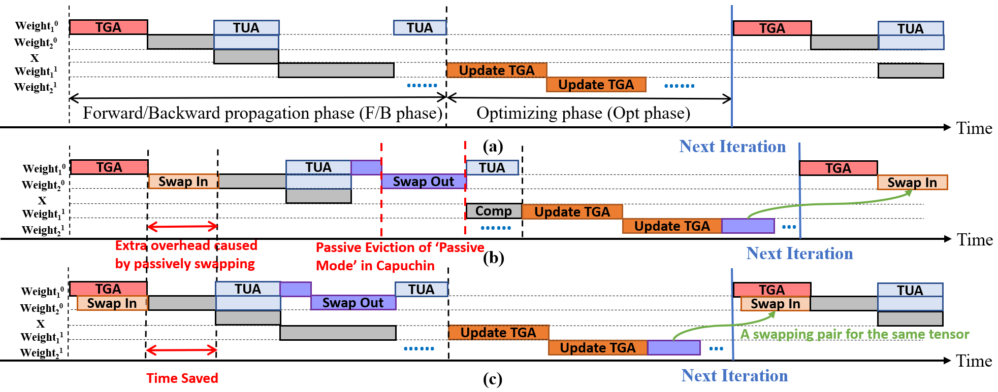
Cold-starting. The most advanced method, such as Capuchin [15] which schedules in tensor granularity, needs to observe the tensor access pattern first before generating the scheduling plan. As shown in Fig. 1(b), such ’Passive Mode’ will cause extra overhead by passively swapping tensors when the GPU memory is insufficient. Also, the multiple workload scenario causes the observation to be inaccurate. So the core challenge is to find a proper way to initialize the tensor access pattern.
-
•
Across-iteration Scheduling. All prior methods only schedule within a single iteration. They ignore that scheduling across iterations is also necessary since some tensors evicted in the current iteration’s Opt phase are used as inputs in the next iteration’s F/B phase, as shown in Fig. 1, which leads to extra overhead. The core challenge is to consider the swapping between two phases.
In this paper, we tackle these challenges and propose TENSILE, a run-time dynamic GPU memory scheduling method of tensor granularity designed to reduce the GPU memory footprint peak towards multiple dynamic workloads.
For the first problem of multi-workloads, we develop a scheduling method that can keep tracking the tensor access latency for updating the scheduling plan to support the multiple dynamic workloads. By updating the scheduling plan in time, the dynamic tensor access patterns caused by multi-workloads scenarios can be well adapted.
To solve the second problem, we use a light neural network model to predict the latency of each operator under current GPU usage. With this model, TENSILE can avoid the extra overhead caused by the ’Passive Mode’.
And for the third problem, our method could schedule tensors across iterations. TENSILE can swap out the parameters at the Opt phase and prefetch them before they are used in the following computation iteration. As the schematic Fig. 1(b, c) shows, such an approach can effectively reduce the total GPU memory peak with less extra overhead of passively swapping and supporting multiple dynamic workloads.
TENSILE is a tensor granularity scheduling approach for supporting deep learning tasks based on tensor computation, such as the training of CNN [18] and GCN [19]. Additionally, we can achieve higher performance with scheduling in tensor granularity since tensor is the most fundamental component of deep learning algorithms. Also, benefiting from the tensor granularity, TENSILE is not limited to the scope of application with forward/backward propagation like most prior works do. It can also handle any tensor computation tasks expressed with tensor operators in a static compute graph.
Our contributions can be concluded as:
-
•
Inspired by existing GPU memory scheduling methods, we proposed a scheduling method toward multiple dynamic workloads. To support such scheduling, we designed a system to track the jobs’ running and manage their memory as a whole, rather than optimizing them separately as previous works did. This method can also schedule the tensors across iterations and reduce the entire process’s GPU memory peak to increase the system’s model capacity.
-
•
We also proposed an innovative algorithm to generate the swapping and recomputation plan based on tensor access sequence, which can support the multiple dynamic workloads better than prior works. With this algorithm, we could initialize the scheduling plan without measuring first and update the scheduling plan in time with the fluctuation of GPU usage.
-
•
According to the experiment results, TENSILE can achieve a higher GPU memory saving rate with less performance loss, especially in multiple dynamic workload scenarios.
II Related Work
In this section, we introduce some prior works in GPU memory management.
NVIDIA is the first organization to pay attention to the GPU management problem. It integrated the Unified Memory technology in CUDA6111https://developer.nvidia.com/blog/unified-memory-in-cuda-6/. This work allows programmers to use the GPU and Host Memory as a unified space. Unlike TENSILE, this work is not specially designed to schedule deep learning processes, which implies programmers need to decide when and which tensor should be swapped with CUDA programming.
In the area of GPU memory scheduling for deep learning, Minsoo Rhu et al. proposed the vDNN [16], which is the first work focusing on scheduling the GPU memory footprint for deep learning processes. The central part of vDNN is an algorithm to decide which layer’s interim result should be released, evicted, or prefetched. Although it is a pioneering work, some problems remain, such as delayed computation start, high pinned memory requirements, and GPU memory fragmentation. Shriram S.B. et al. improved vDNN and solved the three problems mentioned above [20]. By allowing to overlap of the tensor eviction and prefetching process with the computation process, Shriram S.B. et al. significantly improved the vDNN’s performance. Linnan Wang et al. proposed SuperNeurons [17] which is the first dynamic GPU memory run-time management approach. It also introduced recomputation into the scheduling. The authors believe the convolution layer is the most valuable layer to be swapped and designed some approaches to schedule the convolution layers. Although this design helps it to achieve significant efficiency on convolutional networks, it also limits the compatibility for more advanced network structures as transformer [21]. Donglin Yang et al. proposed the first method that supports a unified memory pool for non-linear networks [22]. The method can construct the execution order for non-linear networks based on graph analysis so that it could support non-linear networks better than previous works.
Although all the methods above have significant advantages, they have a major shortcoming compared to TENSILE: all of them are designed to schedule GPU memory in layer granularity. Such a mechanism makes them lack compatibility and unable to save GPU memory as much as tensor granularity methods like TENSILE. This is the fundamental reason why they can not schedule the newest deep learning models that contain complex structures inside a ’layer’ (or as known as ’block’), such as transformer-based networks [21] and the Capsule Network [23]. And the tensors inside the ’layer’ can not be scheduled by these methods, and neither do the interim tensors in the optimizer, such as the and the in the Adam optimizer [24]. These works aim to improve the batch size in a single workload scenario, so only scheduling the tensors in the F/B phase is enough. However, we aim to reduce the memory footprint peak to make the system support more job training simultaneously when it comes to multiple workload scenarios. Moreover, such methods are not good enough since the GPU memory peak will be not only appear in the F/B phase but also in the Opt phase.
In 2019, another method was proposed [25], the first approach that can schedule GPU memory in tensor granularity. This method proposed two orthogonal approaches to reduce the memory cost from the system perspective. It reduces the GPU memory peak by managing the memory pool and scheduling the swapping with a heuristic method. Benefiting from its tensor granularity, this method can support any deep learning network. Xuan Peng et al. proposed Capuchin [15]. Capuchin can observe the tensor access pattern and decide which tensor to be swapped and which to be recomputed with a value-based approach. This method is more flexible in supporting various types of neural networks than those layer granularity methods. However, it highly depends on observing the tensor access pattern when the calculation is running for the first time since the tensor access pattern is needed to generate the scheduling plan. Such observation leads to passive swapping and PCIe channel occupancy when the GPU memory is insufficient.
These two advanced works schedule GPU memory in tensor granularity and solve compatibility problems. However, compared to TENSILE, neither of these prior works can solve the three problems we propose in Section I. We take Capuchin as an example to explain it.
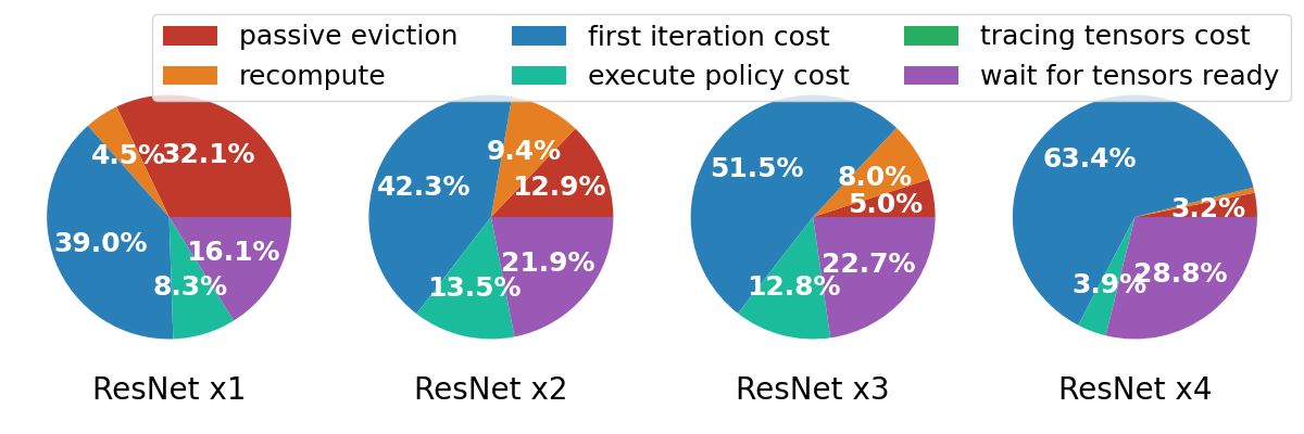
In an environment with multiple workloads, influenced by multiple workloads, the GPU usage fluctuates irregularly, which causes the operators’ latency and tensor access pattern to keep changing, so the scheduling plan must be able to be kept updating iteratively. Capuchin makes a fixed scheduling plan once at the first epoch based on the observed tensor access pattern in the ’Passive Mode’, which is not feasible because the latency of the operator varies with the dynamic load of multiple jobs. Especially when a job launches, the GPU usage will change drastically and cause the initial scheduling plan to lose efficacy. Capuchin has not enough ability to adjust the plan to fit the fluctuation of the tensor access pattern in multiple dynamic workload scenarios. This can be proved by Fig. 2, the time cost of ’wait for tensors ready’ increases with the number of workloads.
The ’Passive Mode’ also causes the cold-starting discussed problem in section I. According to the ’first iteration cost’ of Fig. 2, this unexpected eviction causes the time cost of the first iteration increases since passive swap-out causes the computation to block.
Also, Capuchin and other works above only considered the tensor access in a single iteration. For example, the updated parameters’ accesses at the end of the iteration can not be swapped proactively. Thus, these parameters can only be swapped passively at the next iteration with an additional time overhead. As shown in Fig. 2, the passive eviction takes 32.1% of the overall time cost. Most of these evictions are caused by the memory peak caused by the unexpected swap-in across iterations.
III Overview
This section defines the GPU memory scheduling problem and overviews our deep learning system built to support TENSILE.
III-A Preliminary
For the convenience of scheduling, we use a graph model called static compute graph [26] to describe the tensor calculation jobs. Let be the set of all basic operators to manipulate tensors, be a set of tensors generated by operators in , and be a set of scheduling events, whose elements are {Swap-out, Swap-in, Recompute, Release}. With these symbols, we define the multiple dynamic workload scheduling problem.
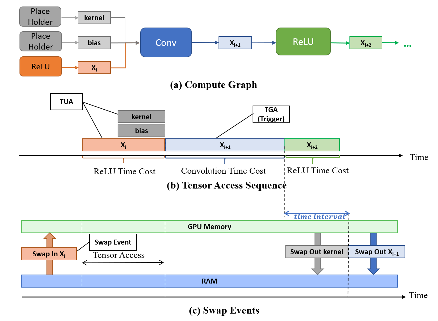
Job: A deep learning job is denoted by a static compute graph as . Note that the graph is a DAG (Direct Acyclic Graph) just like the one in TensorFlow [26], and the operators of the optimizer are also included in . An example of the graph is shown in Fig. 3(a), a convolution operator is represented as a node in the graph. Such a node takes multiple tensors as the input and outputs other tensors. Such a model could effectively represent the computation in modern deep learning frameworks, such as TensorFlow [26].
Tensor Access: For a tensor in , which is generated by the operator and used by the operator , we define the execution of as the Tensor Generating Access(TGA) of and the execution of is the Tensor Using Access(TUA) of . Both tensor accesses are denoted as , where is the access index. Usually, if a given operator is not at the start or the end of a job, it corresponds to two kinds of tensor accesses, the TUA and the TGA. For example, as shown in Fig. 3(b), the convolution operator takes tensors kernel, bias, and generated by the previous operator as inputs and outputs the feature map tensor . The latency of a Tensor Access is defined as the corresponding operator’s execution time cost, which can be inferred from the compute graph or logged at run-time. The TUA is access of the input tensors of , and the TGA represents the accesses of the output tensors of . Additionally, since the operator placeholder generates the input tensors of the whole compute graph, we regard the placeholder as a TGA.
Workload: A workload is denoted by a tensor access sequence ,, which is ordered by the topological order of job . The topological order corresponds to the execution order of operators in . When a workload is launched, the framework executes the operators of in topological order. A dynamic workload has tensor accesses whose latency keeps changing at run time.
Scheduling Plan: We denote a scheduling plan for workload as a sequence of , such as . And for each event , represents that it belongs to the scheduling plan of workload , is its trigger tensor access, which is the prior tensor access of the scheduled event, and is the time interval between the execution end of the trigger tensor access and the start of the scheduling event, just as Fig. 3(c) shows
Memory Footprint: Let function be the GPU memory changing caused by tensor access or scheduling event , the memory footprint of a workload at the end of operator k is
| (1) |
, and the memory footprint peak of workload (with operators) is
| (2) |
The summation process in Equation 1 can be regarded as a discrete GPU memory occupancy change process as the workload’s tensor access sequence is executed. Assuming there are workloads running asynchronously in the system, the global memory footprint peak is .
III-B Problem Definition
With these symbols above, we define the problem here. Let be the GPU memory size, our multiple dynamic workloads scheduling problem is how to generate a scheduling plan for each workload to minimize the global memory footprint peak with as little extra overhead. So that the system with GPU memory can run more neural networks simultaneously or run these given workloads with larger batch sizes for higher efficiency. The optimization goal is formalized as Equation 3 shows.
| (3) |
Note that the interim results and the operators of the optimizer are also included in , and can be scheduled like other tensors, which is different from prior works. Those works are only designed to save GPU memory during the forward/backward propagation to achieve a larger batch size or deeper network. However, our method is designed toward multiple dynamic workloads in the system. The method must reduce the entire job’s GPU memory peak to support multiple workloads, including the peak caused by the optimizer. Otherwise, when two peaks caused by different jobs coincide, an OOM (Out Of Memory) exception will be triggered. Although the exception can be handled by passive swapping just like the Capuchin [15] does, it will cause much extra overhead. This feature is practical, especially when using an optimizer like Adam [24], which will use additional memory twice the size of the parameters.
III-C Concepts Explanation
To facilitate understanding, we explain the basic concepts of TENSILE.
The Tensor Access Sequence is the alias of workload. For each tensor, its Tensor Access Sequence begins with an TGA which generates the tensor and followed by a series of TUA which represents the tensor used by operators as input, as shown in Fig. 1.
A Swap Event transfers data between the GPU and the Host Memory. It has two kinds of types, Swap-Out Event and Swap-In Event. As Fig. 3(c) shows, Swap-Out Event of a tensor will copy the tensor from the GPU memory to the Host Memory and then releases it from the GPU memory as soon as it is not occupied, which can be regarded as eviction. A Swap-In Event will copy a tensor from the Host Memory to the GPU memory, which is used to prefetch the tensor. It is necessary to emphasize that swap-in does not mean the tensor in the Host Memory will be released. On the contrary, it will remain in the Host Memory until the last access of the tensor is finished, which could save much cost of swap-out.
A Recomputation Event regenerates the tensors which have already been released from the GPU memory. For a Tensor Access , we can release it after accessing and recompute it before the Tensor Access that takes the tensor as input.
A Release Event releases the corresponding tensor from the GPU memory as soon as it has not been used.
With these concepts, we can offload tensors when not used and then prefetch or regenerate them by swapping or recomputing them before their TUA.
III-D System Architecture
Since existing approaches cannot schedule among multiple dynamic workloads, we developed a system to support scheduling under such scenarios. The system can collect the necessary information on all the jobs before and during running to support the scheduling algorithm. The information includes the compute graph of jobs, the latency of each operator, and other run-time information such as the GPU utilization. The system will trigger the scheduling algorithm multiple times during startup and running. When receiving the newest scheduling plan, the system will apply it at the next round of iteration. To achieve the functions above, our system contains four components: Global Controller, Memory Scheduler, Executor, and Swap Executor, as shown in Fig. 4.
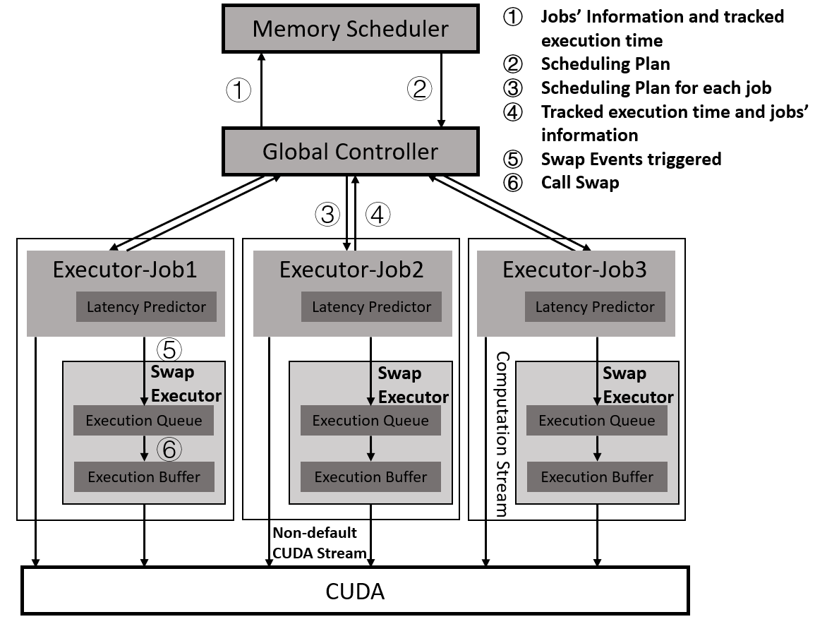
Global Controller. The Global Controller is responsible for launching new jobs’ processes and delivering information between the Executor and the Memory Scheduler. When the user launches a new job, the Global Controller creates a new sub-process of the job’s Executor, and the threads for Swap Executor. It is also responsible for communicating with the Memory Scheduler, and each job’s information is organized and sent to the Memory Scheduler. Also, the scheduling plan of each job is distributed to the corresponding Executor. With the global controller, our system can support the scheduling algorithm described in section IV.
Memory Scheduler. The Memory Scheduler takes the jobs’ information as inputs, such as the compute graph and the operators’ latency tracked by the Executor. Such information is used to generate the Tensor Access Sequence and the scheduling plan, which consists of multiple swapping, releasing, and recomputation instructions. The detailed algorithm will be described in section IV. Each instruction is described by a tuple , the is the previous operator’s end time, and the is the time interval after the trigger. Therefore, the corresponding Swap Event will be triggered in after the , just as the Fig. 3(c) shows. These instructions are grouped by job id and will be distributed to the corresponding Executor by the Global Controller.
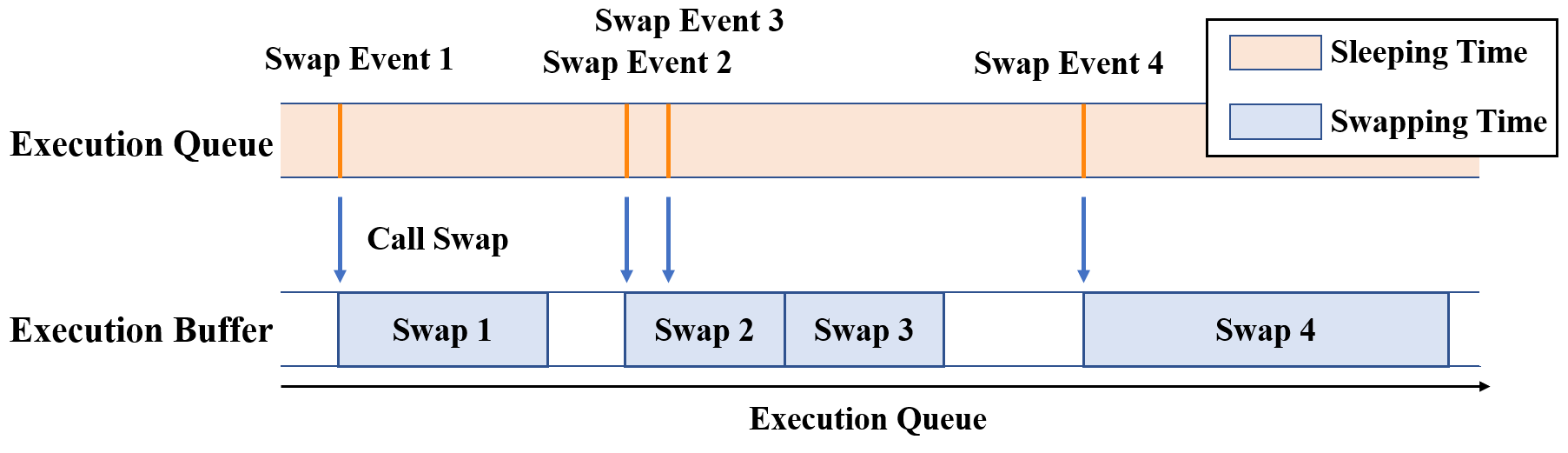
Swap Executor. As Fig. 5 shows, the Swap Executor contains an Execution Queue and an Execution Buffer. The Execution Queue is a thread with an event queue in it. It receives the swap events triggered by a certain operator (trigger tensor) and pushes these swap events into the queue in chronological order. The Execution Queue pops up the swap events to the Execution Buffer for implementing swapping according to their time intervals.
Executor. The Executor executes each operator node in the graph by topological order. For each node, it checks whether all input tensors are in the GPU memory before the computation since the inaccuracy of the estimated Tensor Access Sequence may lead to delays in swapping. If that happens, the Executor will pause the computation and swap the tensors into the GPU memory. When the computation is finished, certain tensors will be released if the Memory Scheduler has set the operator as the release trigger for these tensors. Before releasing, the Executor checks the Swap Executor. The release and computation processes will be blocked if some Swap-Out Events have not been executed. By such a synchronous method, the execution order of swapping, releasing, and computation can be kept. Otherwise, if a given tensor’s Swap-Out Event is executed later than its release, then the data of the tensor will be lost and would cause exceptions.
The Executor also tracks every operator’s latency periodically and sends the information to the Memory Scheduler through the Global Controller for updating the scheduling plan. The Executor will check whether the scheduling plan has been updated each time before a new round of calculation. During the execution of the compute graph, if the scheduling plan requires the current tensor access to trigger some Swap Events, the Executor will send the Swap Event to the Execution Queue of the Swap Executor waiting for execution. At the end of an iteration, the Executor pauses to wait for the unfinished swap events of this iteration.
The system can collect information from each job and execute the corresponding scheduling plan with these components. The whole scheduling procedure has four steps:
-
1.
Collecting the new jobs information through the Global Controller.
-
2.
The Memory Scheduler generates the initial scheduling plan and distributes it to the corresponding job’s Executor through the Global Controller.
-
3.
The Swap Executor executes the scheduling plan during computing. Also, the Executor performs the recomputation events at running.
-
4.
The Executor collects the time cost of each operator and reports to the Global Controller. When the current operators’ latency and the latency used to generate the previous scheduling plan deviate more than the preset threshold, the Global Controller will call the Memory Scheduler to update the scheduling plan based on the newest estimated Tensor Access Sequence.
IV Methods
In this section, we detail our algorithms of TENSILE in the order of actual execution, i.e., Tensor Access Sequence Generation (subsection IV-A), GPU Memory Peak Analysis(subsection IV-B), Swap Event Schedulingsubsection IV-C), Recomputation Scheduling(subsection IV-D), and Scheduling Plan Updating(subsection IV-E).
IV-A Tensor Access Sequence Generation
We first introduce our tensor access sequence generation method since our method is based on GPU memory peak analysis, which depends on tensor access sequence generation. We use a learn-based latency prediction method to solve the cold-starting problem mentioned in Section I. In consideration that there are two pieces of information required to infer the Tensor Access Sequence, which are the Tensor Accesses’ order and the latency of each Tensor Access. We can deal with this problem by diving into two sub-problems of inferring the Tensor Access order and getting each Tensor Access’s latency.
As mentioned above, we execute the operators in the topological order with the compute graph. Therefore, we can solve the first sub-problem and get the Tensor Accesses’ order statically based on each operator’s inputs and outputs. It only solves the first sub-problem, which is inferring the access order. The execution order is unrelated to the latency.
However, accurately predicting the CUDA kernel’s latency is a challenging problem, especially with multiple dynamic workloads.
The most straightforward way to solve the second sub-problem is to run the job with ’Passive Mode’. However, it will cause extra overhead since calculation and swapping can not overlap, and the computation must wait for swapping. To make the initial scheduling plan more efficient, our solution uses pre-trained machine learning models to predict each GPU operator’s latency with the input data size and the current GPU utilization rates. When the system initializes, it will measure each GPU operator’s latency with different input data and GPU usage to generate the training data.
Since the latency of a given operator depends on its inputs’ shape, the parameters such as strides of convolution operator, and the current GPU usage, the inputs of our prediction model are denoted as , where the to denotes the input tensors of the operator, the denotes the i-th dimension’s size of input , the denotes the i-th parameter of the operator, and the denotes the current GPU’s utilization rate. We used a four layers MLP network as the prediction model since the input is not complex, and a simple MLP model is enough to give a relatively precise prediction. According to our experiment, the average MSE of every operator’s prediction result is 4.269, which means that our method can give a relatively precise prediction to most operators. A detailed evaluation of this method’s influence on the scheduling process will be introduced in subsection V-B.
Although the GPU’s utilization rate is a general representation of the GPU usage condition, and the prediction results will not be precisely accurate, we can keep tracking the operators’ latency and dynamically correct the predicted result with the exponential moving weighted average method [27] during the job’s run-time. The details will be introduced in subsection IV-E.
IV-B GPU Memory Peak Analysis
To reduce the entire system’s GPU memory peak, the scheduling algorithm has to know when the GPU memory peak appears and caused by which tensors so that it can try to schedule the Swap Event of these tensors. Thus, with the information inferred from the compute graph, we develop an algorithm to analyze the GPU memory peak statistically.
The algorithm is a discrete simulation process of the Equation 2. According to the Equation 2, the GPU memory footprint is changed only when these five situations happen.
-
1.
Iteration Beginning: At the beginning of a training iteration, these tensors will be in the GPU memory:
-
•
Input data of the model
-
•
Parameters which are not swapped out from the last iteration
-
•
Initial space used by CUDA, cuDNN, and cuBLAS.
These tensors will be used to initialize the GPU memory footprint.
-
•
-
2.
Tensor Generating Access: When a tensor is generated in the GPU memory via , GPU memory footprint increases. Note that when updating a parameter, we logically treat the updated parameter as a new tensor, but the new parameter will not cause an increase in GPU memory footprint since it uses the memory address of the old parameter.
-
3.
Swap-In Event: A Swap-In Event causes GPU memory consumption increase. Since we only concern with the peak of GPU memory footprint, the Swap-In Event’s finishing time point can be regarded as the time point of the GPU memory footprint increases.
-
4.
Swap-Out Event: When a tensor is copied to Host Memory and released, the GPU memory footprint is reduced at the end of the swap-out event (or at the end of the corresponding , if the ends later).
-
5.
Tensor Release: For a Tensor Access which needs to recompute or swap in, when the last Tensor Access -1 finished, the tensor can be released from GPU memory, so that the GPU memory footprint will decrease.
Based on the above discussions, we just need to sort the Tensor Accesses and Swap Events by the time they trigger the GPU memory footprint change. Then we can traverse the job’s timeline to determine the GPU memory peak. We then introduce the analysis algorithm in detail as shown in algorithm 1.
IV-C Swap Event Scheduling
The primary approach in our system to reduce the GPU memory peak is by swapping tensors out to the Host Memory when they are not in use. It is obvious that swapping every tensor out of the GPU memory after their , and swapping them back right before their can save the most GPU memory. However, due to the data transfer occupying the PCIe channels exclusively [15], there can only be one tensor being swapped simultaneously. Therefore, swapping tensors within and between tasks must be scheduled appropriately.
The scheduling process is a deformation of the task scheduling problem with the next two difficulties:
-
•
A Swap Event cannot be executed without prerequisites. For example, a Swap-In Event can be executed if the corresponding Swap-Out Event can be performed. Otherwise, no data will be swapped into the GPU memory. Also, to avoid interrupting task execution, the Swap-Out Event can be executed only when the tensor’s Swap-In Event can be scheduled successfully before the next Tensor Access (we do not allow passively swapping in for performance reasons).
-
•
The scheduling process must be performed considering global jobs’ information, and it needs to be updated frequently due to the dynamic workloads. This fact determines that we can not use a very complex algorithm to generate the scheduling plan. Otherwise, the generation of the scheduling plan will cause significantly extra overheads and makes the scheduling plan can not be updated in time under the fluctuation of GPU utilization.
Facing the difficulties above, we design a greedy algorithm to balance the performance and the time overhead. The main idea is to swap the largest available tensor whose access will cause the GPU memory footprint peak. Since the scheduling for each tensor can change the GPU memory peak, we must analyze the GPU memory peak and generate the swap events iteratively. In particular, the GPU memory peak will be analyzed first based on the Tensor Access Sequence, and choosing the largest tensor that caused the peak to swap. This process is iterated several times until there are no tensors to be scheduled.
With such a greedy algorithm, each scheduled tensor can significantly reduce the GPU memory peak. Now we will detail our algorithm.
We firstly choose the biggest MPT among all jobs as the most valuable tensor to swap (candidate tensor). Note that each job has a max swapping rate limit. Considering the swapping among all jobs, the PCIe channel will be jammed if we swap the tensors in each job as many as possible. Also, we can not control the order of swap events among all jobs because jobs in our system are running asynchronously for performance reasons, and each job’s time cost of one training step is significantly different. If we use a synchronous way to execute these jobs, then there must be extra synchronization overheads. From this perspective, to reduce the conflict opportunity, we define the max swapping rate limit for each job’s tensor swapping as the rate of tensors swapped in a job to tensors swapped in the whole system. It can be regarded as a hyper-parameter. The max swapping rate can be considered the job’s priority. Because the tensors’ swapping can not always overlap with computation with 100 percent odds due to the conflict on PCIe and the changing GPU utilization, swapping implies the job may run slower than usual. In this perspective, a lower swapping rate means higher priority.
After choosing the candidate tensor, each Swap Event’s feasible time intervals will be inferred, as shown in algorithm 2 Line 4 and Lines 23-24, which is defined as its and . There are three bases for inferring the feasible time interval:
-
•
The latest time of the Swap-Out Event cannot be later than the time the GPU memory peak appears since we want to swap it to reduce the GPU memory peak. Furthermore, a Swap-Out Event must start after its .
-
•
A Swap-In Event cannot be earlier than the corresponding Swap-Out Event or later than the that uses it as input. Therefore, our algorithm needs to decide the start time of each event under the constraint of its feasible time intervals.
-
•
The Swap Event can not overlap with the corresponding tensor’s access.
Based on the feasible time intervals, we choose the available intervals greedily. For a Swap-Out Event, it will start as early as possible, and for a Swap-In Event, it will start as late as possible so that we can save the GPU memory occupied by the tensor for a longer time. If there are no available intervals, then we will break the outer loop in Line 20 and try to swap the following tensor.
Next, we have to decide when to execute the Swap-Out Event and the Swap-In Event. Since the tensors in the forward/backward propagation phase and the optimizing phase have different constraints, we will introduce them separately.
The tensors in the forward/backward propagation phase must be swapped into the GPU before the first after the Swap-Out Event. Otherwise, an exception will be triggered due to missing necessary input tensors, and the system has to pause the computation to wait for their swapping. As shown in algorithm 2 Lines 10-14, we look for the first after the Swap-Out Event and generate the Swap-In Event and its feasible intervals to see whether any of these intervals can cover the Swap-In Event. If they can not cover the event, we will update the Swap-Out Event’s earliest start time and regenerate the feasible intervals(Lines 18-19). Otherwise, for the rest of the tensor, we try to swap them in as much as possible(Line 34). If a Swap Event is scheduled successfully, the corresponding tensor can be released after the previous is finished. TENSILE will also analyze the compute graph and release the tensors after their last access(Activity Analysis). The detailed algorithm of swapping scheduling is shown in algorithm 2.
Most prior works ignore the tensors which need to be updated in the Opt phase. This causes the ’Across-iteration Scheduling’ problem. TENSILE solves this problem with the following rules: if these tensors are swapped out at the optimizing phase, the corresponding tensors must be swapped in at the beginning of the next iteration. As shown in algorithm 2 Lines 8-9 and Line 27, it tries to swap out the updated tensors and then swaps in the corresponding tensor before the first . Fig. 1(c) shows this process more vividly.
With this algorithm, we can select the most valuable tensors to be appropriately scheduled among all jobs, thus reducing the entire computation job’s GPU memory peak.
IV-D Recomputation Scheduling
If the predicted GPU memory peak is still larger than the GPU memory after swapping scheduling, we need to use recomputation to save more GPU memory. However, a major shortcoming of recomputation is that it will add extra and change the Tensor Access Sequence. If the inputs of a recomputation have been swapped out or released, then it needs to be swapped in or recomputed, which will disrupt the swapping plan just generated and cause much more time overhead. Therefore, we will only apply recomputation on those tensor accesses which have never been released. To achieve the best GPU memory saving effect, we will select those accesses that conform to the above conditions with the largest recomputation value until the GPU memory is enough to run these jobs.
To measure a recomputation’s value, we used the metric proposed in Capuchin [15], known as MSPS. This metric can measure the memory saving and extra time cost at the same time.
| (4) |
IV-E Scheduling Plan Updating
As discussed in section I, each operator’s latency changes along with the jobs’ running in the multiple dynamic workloads scenarios. This leads to a changing Tensor Access Sequence, so the initial scheduling plan based on the outdated Tensor Access Sequence will be less efficient. For example, the hit rate of Swap-In Event will decrease and causes an increasing extra overhead. To adapt to such kinds of dynamic workloads, the Memory Scheduler needs to be able to update the scheduling plan based on the operators’ latency collected by the Executor.
Two major problems should be solved.
-
1.
When should the scheduling plan needs to be updated?
-
2.
How to update the scheduling plan?
Since the reason for updating the scheduling plan is that the latency of operators has been significantly changed compared to the time used to generate the last Tensor Access Sequence, we only need to propose a metric to measure this change. We use the average latency rate of change, which is defined as , where is the newest sum of each operation’s latency, and is the last sum of each operation’s latency. If the changing rate is larger than the updating threshold set before, then the updating of the scheduling plan will be triggered.
To correct the Tensor Access Sequence and make the scheduling plan more accurate, we use the exponential weighted moving average algorithm[27] to update the latency of operators. By predicting and correcting the latency, TENSILE can achieve higher performance than Capuchin’s ’Passive Mode’ since passively swapping tensors requires extra overhead.
IV-F Discussion of supporting Dynamic Workload and the range of application
With algorithm 1, TENSILE can give a more effective initial scheduling plan than the ’Passive Mode.’ The system will keep tracing recent tensor accesses time to correct the Tensor Access Sequence and update the scheduling plan. When a job is launched, the Tensor Access Sequences of other jobs are most likely to fluctuate greatly. In this situation, TENSILE updates the Tensor Access Sequence based on current GPU usage for all jobs. To avoid extra overhead caused by scheduling plan changes, the system will apply the new plan before computing the next batch of data. The complete scheduling algorithm is shown in algorithm 3. Firstly, we run an activity analysis at the beginning of the scheduling to save more memory. Every tensor will be released when its last TUA is finished. Then, the Memory Scheduler will iteratively run the process below until no swapping or recomputation is scheduled. At each iteration, the algorithm will start with running the GPU_Memory_Peak_Analysis function for each job and merge the result as shown in Lines 6-7. Then, if at least one swap event is scheduled successfully in the previous iteration, it will keep trying to swap, as shown in Lines 8-12. Otherwise, if the GPU memory is insufficient, it will try to schedule the recomputation events as shown in Lines 13-15.
Although our method is designed to run on a single GPU, it can also support data-parallel models for multiple GPUs in the cluster. In this situation, the scheduling processes are the same with a single GPU situation on each node, with the premise that its CPU has enough PCIe channels for the GPUs to use in a single node.
V Experiments
To verify the effectiveness of the proposed approaches, we conduct extensive experiments in this section.
V-A Methodology
Experiment Platform. To apply our scheduling algorithm, we implement a naive deep learning framework with CUDA as our experiment platform. The framework is modified based on the tinyflow open-source project222https://github.com/LB-Yu/tinyflow. We also reproduce vDNN [16], and Capuchin [15] coupling with our framework based on their papers.
Baselines. We choose two methods as baselines from layer-granularity and tensor-granularity methods to compare with our method. The first one is vDNN, which swaps out the appropriate feature maps and uses a static swap-in strategy for prefetching. There are two types vDNNs, vDNNall and vDNNconv, the former tries to swap every feature map, and the latter only swaps the feature maps of convolution layers. We take the vDNNconv as one of our baselines since the authors of vDNN proved that vDNNconv has much higher performance than vDNNall [16]. The second baseline is Capuchin, the newest and the most representative dynamic scheduling method in tensor granularity for a single job. Although these baselines are designed for single workload scenarios, we can also create an instance for each workload in our experiments and schedule each workload independently. And both the baselines and our method overlap data transfer and computation with cudaMemcpyAsync.
Metrics. We introduce the metrics used to evaluate the performance of TENSILE. We choose Memory Saving Rate(MSR), Extra Overhead Rate(EOR), and Cost-Benefit Rate(CBR) to measure the TENSILE’s performance and efficiency compared to the baselines. Their definitions are shown as follows:
; ; .
Where and are the memory footprint peak of the vanilla group (no scheduling) and the experimental group (TENSILE or baselines), and are the time cost of the vanilla group and the experimental group.
The three metrics we choose are the key metrics to evaluate a GPU memory scheduling method. The Memory Saving Rate (MSR) represents how much GPU memory a scheduling method can save compared to the vanilla method (no scheduling), the higher implies that the corresponding scheduling method can reduce more GPU memory footprint peak compared to the vanilla method. The EOR indicates how many times the time cost will be caused by saving these proportions of GPU memory. The lower implies that the scheduling method has less extra overhead. The CBR is the ratio of MSR and EOR, which indicates how much extra overhead it takes to save a piece of GPU memory. The higher implies that the corresponding scheduling method is more space-time efficient than other methods. These metrics are common and fair for TENSILE and both baselines since we analyzed and compared the MSR, EOR, and CBR of the whole computing process of TENSILE and both baselines in detail. Since TENSILE is designed for multiple dynamic workload scenarios, it is expected to have higher and and less compared to other baseline methods.
Statement of our reproduction. It is necessary to emphasize that the reproduction for Capuchin may not be exactly the same as its authors’ implementation in the paper [15] in the aspect of the system framework since there is no source code to refer to, and it is implemented in TensorFlow. For example, in Capuchin, they measure the GPU kernel latency through CUPTI. However, in our platform, every computation will be synchronized between CPU and GPU, so we can measure the operators’ latency in the python codes. We want to compare the scheduling algorithm that runs on the same platform rather than whose platform implementation is more computationally efficient. Therefore, the experiments will be fair since all the methods’ scheduling algorithms are implemented exactly as their paper described and run on the same platform for comparison.
Experiment Platform. Our experiment is conducted on a server that has Intel(R) Xeon(R) Silver 4210R CPU, 504GB Host Memory, and one RTX A6000 with 48GB memory. The system version is Ubuntu 18.04 with GCC 7.5.0, the CUDA version is 11.3, the cuDNN is 8.2.0, and Python 3.10.
Workloads. We choose the five neural networks in the evaluation of the Capuchin[15] to evaluate TENSILE, VGG-16 [28], InceptionV3 [29], InceptionV4 [30], ResNet-50 [2], and DenseNet [31], covered both linear network and non-linear network. We will increase the workload number on one GPU and measure the GPU memory footprint and the extra time overhead for each method.
Extra Setting. The Capuchin is designed to schedule only when the GPU memory is insufficient. It will only save the GPU memory to the threshold that is just able to run the workloads, which makes it difficult to compare its performance with TENSILE since TENSILE is a more active scheduling method that will save GPU memory as much as possible. Therefore, we set Capuchin’s GPU memory budget as the same as TENSILE. Then we can compare these two methods’ time cost and efficiency fairly.
Also, our method includes two phases, the cold start phase, and the dynamic updating phase. The former uses predicted operations’ latency to generate the schedule plan before the job launching, and the latter updates the scheduling plan with the running information collected from the framework. To analyze these two phases separately, we denote the cold start phase by and the updating phase by . The ’s performance is measured once the job is launched, and the ’s performance is measured once the scheduling plan is updated. We also use to denote the whole process of TENSILE.
V-B Performance of TENSILE’s Each Phase
We first evaluate the performance of the cold start phase and the update phase of TENSILE by measuring the memory footprint and time cost separately. The results are shown in Table I.
| Workloads | Phase | MSR | EOR | CBR |
|---|---|---|---|---|
| VGG-16 | 0.2670 | 1.6287 | 0.1639 | |
| 0.2670 | 6.0128 | 0.0444 | ||
| 0.3192 | 1.2475 | 0.2559 | ||
| InceptionV3 | 0.4361 | 1.6468 | 0.2648 | |
| 0.4361 | 3.1128 | 0.1401 | ||
| 0.4788 | 1.4839 | 0.3227 | ||
| InceptionV4 | 0.5154 | 1.4281 | 0.3609 | |
| 0.5154 | 2.6727 | 0.1929 | ||
| 0.5558 | 1.2898 | 0.4309 | ||
| ResNet-50 | 0.4258 | 1.5540 | 0.2740 | |
| 0.4258 | 3.5395 | 0.1203 | ||
| 0.4647 | 1.3813 | 0.3364 | ||
| DenseNet | 0.5135 | 1.1678 | 0.4397 | |
| 0.5135 | 2.2532 | 0.2279 | ||
| 0.5236 | 1.0664 | 0.4910 |
The MSR of equals the metric of , which proves that the cold start phase is the bottleneck of the whole process of TENSILE. Also, compared to Capuchin’s performance in Table III, can achieve a similar performance as Capuchin with the prediction method only. This result proves the effectiveness of our prediction method. Note that the time cost of the cold start phase includes the overhead of the prediction of the MLP models, and this result proves the effectiveness of the scheduling plan updating method. Furthermore, benefiting from the scheduling plan updating method in subsection IV-E, the update phase’s MSR and EOR are significantly higher than the cold start phase. Since the plan updating method takes the main ingredient, its high efficiency significantly reduces the overhead of the entire computing process.
We also measure the first iteration of TENSILE and Capuchin to compare the EOR of our MLP-based prediction method with the ’Passive Mode’ of Capuchin. The results are shown in Table II, which shows that TENSILE has a more efficient method for the cold-starting situation. For the MLP latency prediction models’ memory cost, our method contains 40 models, and the size of their parameters is 321MB.
| Workloads | Method | EOR | Prediction Cost(s) | Prediction EOR |
|---|---|---|---|---|
| VGG-16 | 1.2523 | 1.3549 | 0.2067 | |
| 5.8053 | - | - | ||
| InceptionV3 | 1.4744 | 1.4743 | 0.3699 | |
| 6.7529 | - | - | ||
| InceptionV4 | 1.3797 | 2.4991 | 0.2865 | |
| 10.2088 | - | - | ||
| ResNet-50 | 1.3924 | 1.7823 | 0.3198 | |
| 9.6073 | - | - | ||
| DenseNet | 1.3855 | 1.3855 | 0.3335 | |
| 10.0925 | - | - |
V-C Single Workload Performance
We compare TENSILE’s performance with vDNN and Capuchin on a single workload. The batch size is set to 16. And for TENSILE, the max swapping rate limit is set to 100% for each task since there is only one task in this experiment. The result is shown in Table III.
And the result also shows that our method can save 26.70%-51.54% memory than the vanilla method, which is much higher than vDNN. This is foreseeable since TENSILE is a tensor granularity scheduling method. And the cost-benefit rate of TENSILE is also much higher than vDNN and Capuchin, which proves the efficiency of TENSILE.
The high efficiency of TENSILE is due to the fact we put the extra time cost into priority consideration, which is embodied in that we do not allow the non-overlapping between swapping and computation logically. On the contrary, the other baseline methods allow the computation to wait for swapping when scheduling. Also, compared to Capuchin, TENSILE can schedule tensors across iterations. This feature helps to avoid some passive swap-in.
This result proves that although TENSILE is designed for multiple jobs and dynamic workloads, it can still achieve the best efficiency and memory saving rate in a single workload situation.
| Workloads | Methods | MSR | EOR | CBR |
|---|---|---|---|---|
| VGG-16 | vDNN | 0.1109 | 1.7835 | 0.0622 |
| Capuchin | 0.2558 | 1.8304 | 0.1398 | |
| 0.2670 | 1.6287 | 0.1639 | ||
| InceptionV3 | vDNN | 0.1633 | 2.5184 | 0.0648 |
| Capuchin | 0.4331 | 2.7745 | 0.1561 | |
| 0.4361 | 1.6468 | 0.2648 | ||
| InceptionV4 | vDNN | 0.1903 | 2.5028 | 0.0760 |
| Capuchin | 0.5129 | 3.2362 | 0.1585 | |
| 0.5154 | 1.4281 | 0.3609 | ||
| ResNet-50 | vDNN | 0.1733 | 2.2981 | 0.0754 |
| Capuchin | 0.3859 | 2.2320 | 0.1729 | |
| 0.4258 | 1.5540 | 0.2740 | ||
| DenseNet | vDNN | 0.1381 | 2.6148 | 0.0528 |
| Capuchin | 0.4860 | 3.4400 | 0.1413 | |
| 0.5135 | 1.1678 | 0.4397 |
V-D Scalability
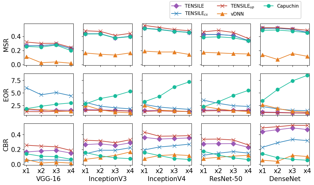
To evaluate our method’s performance on multiple dynamic workloads and test its scalability, we choose one to four workloads respectively and launch them simultaneously to simulate a multiple dynamic workloads scenario. We repeat each test three times and report the average metric in Fig. 6.
As the Fig. 6 shows, in most of the workloads, TENSILE has achieved the best MSR and CBR, which is solid proof of the performance of TENSILE in multiple dynamic workloads situations. The EOR and CBR of do not outperform Capuchin in VGG-16 since the VGG-16 has a massive tensor generated by a wide MLP layer, which causes it much harder to schedule without the overhead. TENSILE tackles this problem by the updating method, and the whole TENSILE, including the updating phase, outperforms Capuchin. With the increased workload, TENSILE’s MSR of InceptionV3, InceptionV4, ResNet-50, and DenseNet drops slowly. And in all experiments, saves the most GPU memory.
Furthermore, according to the EOR metric, Capuchin’s overhead dramatically increases as we analyze in the last paragraph of section II. The VDNN’s EOR reduces with the increasing workload numbers since the VDNN is a layer-granularity method, which can not schedule all tensors so it has many free time intervals for swapping. This makes its extra time cost less than the vanilla method’s time cost. And with increasing workload numbers, the vanilla time cost rises faster than the extra time cost. So the EOR gets lower. Although VDNN has a lower overhead in multiple workload scenarios, its MSR is meager compared to TENSILE and Capuchin.
In any case, the efficiency of TENSILE is still much higher than both baselines. Moreover, the ratios of TENSILE’s CBR to vDNN/Capuchin’s CBR under the multi-workload environment are higher than in the single-workload environment. The conclusion is that TENSILE can run these workloads with less (or at least the same) GPU memory and time cost than baselines. Especially compared to the Capuchin, whose EOR is significantly increasing when the number of workloads increases, which implies most of their swapping transfer can not overlap with the computation, TENSILES’s EOR is much more stable. This experiment strongly proves that the performance of TENSILE is much better than vDNN and Capuchin in multiple dynamic workloads scenarios. To evaluate our method’s performance on multiple dynamic workloads and test its scalability, we choose one to four workloads respectively and launch them simultaneously to simulate a multiple dynamic workloads scenario. We repeat each test three times and report the average metric in Fig. 6.
V-E Mixed Neural Architectures
To measure the TENSILE’s performance in a mixed neural architectures workloads scenario, we randomly launch the five above workloads and measure the total GPU memory footprint and execution overhead. The five workloads are launched one by one in random order, and this procedure is repeated three times. We set the budget of each workload of Capuchin with the MSR of TENSILE in Table IV.
As Table IV shows, TENSILE is comprehensively leading in EOR and CBR under different neural architectures. It can save much more GPU memory with less extra cost in scenarios with complex non-linear workloads, making it more suitable for environments such as in-database machine learning.
V-F Overhead Analysis
Although TENSILE outperforms two baselines, the overheads during GPU memory scheduling can hardly be avoided completely.
For single workloads scenarios, the overheads are caused by two reasons. The first reason is that when the memory is extremely insufficient, the overhead of passive swap-in and recomputation cannot be avoided completely. However, using a more efficient scheduling algorithm, TENSILE achieves less overhead than Capuchin. The second reason is the failed tensor prefetch caused by the fluctuation of GPU operator latency and the error of estimated operator latency.
For multiple workloads scenarios, the GPU utilization rate and the PCIe channel are all influenced by the asynchronous workloads, which makes the prefetch much harder and makes more passive swap-in and recomputation. TENSILE alleviates this problem by choosing the most valuable tensors among all workloads to schedule to achieve higher efficiency. However, it is not a perfect solution, and we will continue to find better solutions to this problem in the future.
| Methods | MSR | EOR | CBR |
|---|---|---|---|
| vDNN | 0.0580 | 1.6297 | 0.0356 |
| Capuchin | 0.1150 | 7.6545 | 0.0150 |
| TENSILE | 0.1565 | 1.1589 | 0.1350 |
V-G Influence of Batch Size
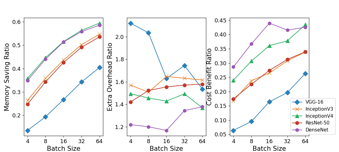
We also analyzed the batch size’s influence on our method by running those five workloads, respectively, with batch sizes 4, 8, 16, 32, and 64. The results are shown in Fig. 7.
The MSR increases with the batch size for all workloads, and so does their CBR in general. This result shows that the TENSILE can save more GPU memory with less overhead when the batch size increases. This result proves that TENSILE is more effective in scheduling the interim results than the parameters since the former is the only one influenced by the batch size. The DenseNet with batch size 32 and 64 is an exception. We believe it is because there are too many tensors to swap. And when the batch size increases, the swap events can more easily conflict with each other. And for VGG-16, it is the only workload whose EOR drops with the increase in batch size. This is because that VGG-16 has a wide MLP layer that outputs a huge tensor. This tensor’s computation cost increases faster than its scheduling cost, so the EOR gets lower.
VI Conclusions & Future Work
We propose TENSILE, a tensor granularity GPU memory scheduling method toward multiple dynamic workload scenarios. TENSILE has solved three major problems of prior works, multiple dynamic workloads, cold-starting, and across-iteration scheduling by designing a scheduling method and corresponding system, a latency prediction method, and a scheduling algorithm. Furthermore, TENSILE is a generic scheduling method for computing tasks described as DAGs, especially deep learning tasks. The experiment results show that TENSILE can achieve much higher performance in such scenarios than vDNN and Capuchin. Even in single workload scenarios, TENSILE can still outperform baselines. These features can help systems such as in-database machine learning run more deep learning tasks with tiny extra overhead.
Acknowledgment
This paper was supported by NSFC grant (62232005).
References
- [1] S. Dargan, M. Kumar, . Maruthi, M. R. Ayyagari, and . Kumar, “A survey of deep learning and its applications: A new paradigm to machine learning,” 07 2019.
- [2] K. He, X. Zhang, S. Ren, and J. Sun, “Deep residual learning for image recognition,” 2016 IEEE Conference on Computer Vision and Pattern Recognition (CVPR), pp. 770–778, 2016.
- [3] J. Devlin, M.-W. Chang, K. Lee, and K. Toutanova, “Bert: Pre-training of deep bidirectional transformers for language understanding,” in NAACL-HLT, 2019.
- [4] T. Brown, B. Mann, N. Ryder, M. Subbiah, J. Kaplan, P. Dhariwal, A. Neelakantan, P. Shyam, G. Sastry, A. Askell, S. Agarwal, A. Herbert-Voss, G. Krüger, T. Henighan, R. Child, A. Ramesh, D. Ziegler, J. Wu, C. Winter, C. Hesse, M. Chen, E. Sigler, M. Litwin, S. Gray, B. Chess, J. Clark, C. Berner, S. McCandlish, A. Radford, I. Sutskever, and D. Amodei, “Language models are few-shot learners,” ArXiv, vol. abs/2005.14165, 2020.
- [5] D. Yang and D. Cheng, “Efficient gpu memory management for nonlinear dnns,” in Proceedings of the 29th International Symposium on High-Performance Parallel and Distributed Computing, ser. HPDC ’20. New York, NY, USA: Association for Computing Machinery, 2020, p. 185¨C196. [Online]. Available: https://doi.org/10.1145/3369583.3392684
- [6] V. Narasayya, I. Menache, M. Singh, F. Li, M. Syamala, and S. Chaudhuri, “Sharing buffer pool memory in multi-tenant relational database-as-a-service,” Proc. VLDB Endow., vol. 8, pp. 726–737, 2015.
- [7] T. Li, J. Zhong, J. Liu, W. Wu, and C. Zhang, “Ease.ml: Towards multi-tenant resource sharing for machine learning workloads,” Proc. VLDB Endow., vol. 11, pp. 607–620, 2018.
- [8] B. Karlas, J. Liu, W. Wu, and C. Zhang, “Ease.ml in action: Towards multi-tenant declarative learning services,” Proc. VLDB Endow., vol. 11, pp. 2054–2057, 2018.
- [9] S. Boag, P. Dube, K. El Maghraoui, B. Herta, W. Hummer, K. R. Jayaram, R. Khalaf, V. Muthusamy, M. Kalantar, and A. Verma, “Dependability in a multi-tenant multi-framework deep learning as-a-service platform,” in 2018 48th Annual IEEE/IFIP International Conference on Dependable Systems and Networks Workshops (DSN-W), 2018, pp. 43–46.
- [10] W. Xiao, R. Bhardwaj, R. Ramjee, M. Sivathanu, N. Kwatra, Z. Han, P. Patel, X. Peng, H. Zhao, Q. Zhang, F. Yang, and L. Zhou, “Gandiva: Introspective cluster scheduling for deep learning,” in Proceedings of the 13th USENIX Conference on Operating Systems Design and Implementation, ser. OSDI’18. USA: USENIX Association, 2018, p. 595¨C610.
- [11] D. Narayanan, K. Santhanam, F. Kazhamiaka, A. Phanishayee, and M. A. Zaharia, “Heterogeneity-aware cluster scheduling policies for deep learning workloads,” in OSDI, 2020.
- [12] R. Marcus, P. Negi, H. Mao, C. Zhang, M. Alizadeh, T. Kraska, O. Papaemmanouil, and N. Tatbul, “Neo: a learned query optimizer,” Proceedings of the VLDB Endowment, vol. 12, pp. 1705–1718, 07 2019.
- [13] R. Marcus, P. Negi, H. Mao, N. Tatbul, M. Alizadeh, and T. Kraska, “Bao: Making learned query optimization practical,” 06 2021, pp. 1275–1288.
- [14] T. Kraska, A. Beutel, E. Chi, J. Dean, and N. Polyzotis, “The case for learned index structures,” 05 2018, pp. 489–504.
- [15] X. Peng, X. Shi, H. Dai, H. Jin, W. Ma, Q. Xiong, F. Yang, and X. Qian, “Capuchin: Tensor-based gpu memory management for deep learning,” Proceedings of the Twenty-Fifth International Conference on Architectural Support for Programming Languages and Operating Systems, 2020.
- [16] M. Rhu, N. Gimelshein, J. Clemons, A. Zulfiqar, and S. W. Keckler, “vdnn: Virtualized deep neural networks for scalable, memory-efficient neural network design,” 2016 49th Annual IEEE/ACM International Symposium on Microarchitecture (MICRO), pp. 1–13, 2016.
- [17] L. Wang, J. Ye, Y. Zhao, W. Wu, A. Li, S. Song, Z. Xu, and T. Kraska, “Superneurons: dynamic gpu memory management for training deep neural networks,” ACM SIGPLAN Notices, vol. 53, pp. 41–53, 02 2018.
- [18] A. Krizhevsky, I. Sutskever, and G. E. Hinton, “Imagenet classification with deep convolutional neural networks,” Commun. ACM, vol. 60, no. 6, p. 84¨C90, May 2017. [Online]. Available: https://doi.org/10.1145/3065386
- [19] T. N. Kipf and M. Welling, “Semi-supervised classification with graph convolutional networks,” CoRR, vol. abs/1609.02907, 2016. [Online]. Available: http://arxiv.org/abs/1609.02907
- [20] B. ShriramS, A. Garg, and P. Kulkarni, “Dynamic memory management for gpu-based training of deep neural networks,” 2019 IEEE International Parallel and Distributed Processing Symposium (IPDPS), pp. 200–209, 2019.
- [21] A. Vaswani, N. Shazeer, N. Parmar, J. Uszkoreit, L. Jones, A. N. Gomez, u. Kaiser, and I. Polosukhin, “Attention is all you need,” in Proceedings of the 31st International Conference on Neural Information Processing Systems, ser. NIPS’17. Red Hook, NY, USA: Curran Associates Inc., 2017, p. 6000¨C6010.
- [22] D. Yang and D. Cheng, “Efficient gpu memory management for nonlinear dnns,” in Proceedings of the 29th International Symposium on High-Performance Parallel and Distributed Computing, ser. HPDC ’20. New York, NY, USA: Association for Computing Machinery, 2020, p. 185¨C196. [Online]. Available: https://doi.org/10.1145/3369583.3392684
- [23] S. Sabour, N. Frosst, and G. E. Hinton, “Dynamic routing between capsules,” in Proceedings of the 31st International Conference on Neural Information Processing Systems, ser. NIPS’17. Red Hook, NY, USA: Curran Associates Inc., 2017, p. 3859¨C3869.
- [24] D. Kingma and J. Ba, “Adam: A method for stochastic optimization,” International Conference on Learning Representations, 12 2014.
- [25] J. Zhang, S. H. Yeung, Y. Shu, B. He, and W. Wang, “Efficient memory management for gpu-based deep learning systems,” arXiv preprint arXiv:1903.06631, 2019.
- [26] M. Abadi, P. Barham, J. Chen, Z. Chen, A. Davis, J. Dean, M. Devin, S. Ghemawat, G. Irving, M. Isard et al., “Tensorflow: A system for large-scale machine learning,” in 12th USENIX symposium on operating systems design and implementation (OSDI 16), 2016, pp. 265–283.
- [27] M. Perry, The Exponentially Weighted Moving Average, 06 2010.
- [28] K. Simonyan and A. Zisserman, “Very deep convolutional networks for large-scale image recognition,” in 3rd International Conference on Learning Representations, ICLR 2015, San Diego, CA, USA, May 7-9, 2015, Conference Track Proceedings, Y. Bengio and Y. LeCun, Eds., 2015. [Online]. Available: http://arxiv.org/abs/1409.1556
- [29] C. Szegedy, V. Vanhoucke, S. Ioffe, J. Shlens, and Z. Wojna, “Rethinking the inception architecture for computer vision,” 2016 IEEE Conference on Computer Vision and Pattern Recognition (CVPR), pp. 2818–2826, 2016.
- [30] C. Szegedy, S. Ioffe, V. Vanhoucke, and A. Alemi, “Inception-v4, inception-resnet and the impact of residual connections on learning,” AAAI Conference on Artificial Intelligence, 02 2016.
- [31] G. Huang, Z. Liu, and K. Q. Weinberger, “Densely connected convolutional networks,” CoRR, vol. abs/1608.06993, 2016. [Online]. Available: http://arxiv.org/abs/1608.06993