Coarse-Grid Selection Using Simulated Annealing

Abstract

Multilevel techniques are efficient approaches for solving the large linear systems that arise from discretized partial differential equations and other problems. While geometric multigrid requires detailed knowledge about the underlying problem and its discretization, algebraic multigrid aims to be less intrusive, requiring less knowledge about the origin of the linear system. A key step in algebraic multigrid is the choice of the coarse/fine partitioning, aiming to balance the convergence of the iteration with its cost. In work by MacLachlan and Saad [1], a constrained combinatorial optimization problem is used to define the “best” coarse grid within the setting of a two-level reduction-based algebraic multigrid method and is shown to be NP-complete. Here, we develop a new coarsening algorithm based on simulated annealing to approximate solutions to this problem, which yields improved results over the greedy algorithm developed previously. We present numerical results for test problems on both structured and unstructured meshes, demonstrating the ability to exploit knowledge about the underlying grid structure if it is available.

1 Introduction

Multigrid and other multilevel methods are well-established algorithms for the solution of large linear systems of equations that arise in many areas of computational science and engineering. Multigrid methods arise from the observation that basic iterative methods, such as the (weighted) Jacobi and Gauss-Seidel iterations, effectively eliminate only part of the error in an approximation to the solution of the problem, and that the complementary space of errors can be corrected from a coarse representation of the problem. While geometric multigrid has been shown to be highly effective for problems where a hierarchy of discrete models can be built directly, many problems benefit from the use of algebraic multigrid (AMG) techniques, where graph-based algorithms and other heuristics are used to define the multigrid hierarchy directly from the matrix of the finest-grid problem.

First introduced in the early 1980’s [2, 3], AMG is now widely used and available in standard libraries, such as hypre [4, 5], PETSc [6, 7], Trilinos [8, 9], and PyAMG [10]. While there are many variants of AMG (as discussed below), the common features of AMG algorithms are the use of graph-based algorithms to construct a coarse grid from the given fine-grid discretization matrix (possibly with some additional information, such as geometric locations of the degrees of freedom for elasticity problems [11]) followed by construction of an algebraic interpolation operator from the coarse grid to the fine grid. Both of these components have received significant attention in the literature, with an abundance of schemes for creating the coarse grid and for determining the entries in interpolation. In this paper, we focus on the coarse-grid correction process, adopting a combinatorial optimization viewpoint on the selection of coarse-grid points in the classical AMG setting.

One of the primary differences between so-called classical (Ruge-Stüben) AMG and (smoothed) aggregation approaches is in how the coarse grid itself is defined [12]. In aggregation-based approaches, coarse grids are defined by clustering fine-grid points into aggregates (or subdomains), while, in classical AMG, a subset of the fine-grid degrees of freedom (points) is selected in order to form the coarse grid. In the original method [3, 13], this was accomplished using a greedy algorithm to construct a maximal independent set over the fine-grid degrees of freedom as a “first pass” at forming the coarse-grid set, which is then augmented by a “second pass” algorithm that ensures suitable interpolation can be defined from the final coarse grid. Many alternative strategies to forming the coarse grid have been proposed over the years, particularly for the parallel case, to overcome the inherent sequentiality of the original algorithm [14, 15, 5, 16, 17]. Other approaches, for example based on redefining the notion of strength of connection [18, 19, 20, 21] or use of compatible relaxation principles [22, 23], have also been proposed.

Much of this work has been motivated by the failure of the classical AMG heuristics to yield robust solvers for difficult classes of problems, such as the Helmholtz equation, convection-dominated flows, or coupled systems of PDEs. While much research has tried to generalize these heuristics to give sensible algorithms for broader classes of problems, another approach is to consider methods that abandon these heuristics in favour of algorithms that are directly tied to rigorous multigrid convergence theory. In recent years, two main classes of AMG algorithms have arisen in this direction. One class of methods arises in the aggregation setting, where well-chosen pairwise aggregation algorithms coupled with suitable relaxation can yield convergence guarantees for symmetric, diagonally dominant M-matrices [24, 25]. The second class of methods are those based on reduction-based AMG principles, where there is a direct connection between properties of the fine-grid submatrix and the guaranteed convergence rate of the scheme [26, 1, 27, 28]. Reduction-based multigrid methods [29] are a generalization of cyclic reduction [30], in which conditions on the coarse/fine partitioning are relaxed so that while the exact Schur complement may not be sparse, it can be accurately approximated by a sparse matrix. This notion is made rigorous by MacLachlan et al. [26], who propose a theoretical framework to analyze convergence based on diagonal dominance of the fine-grid submatrix (in contrast to the fine-grid submatrix being diagonal in the classical setting of cyclic reduction), and extended to Chebyshev-style relaxation schemes by Gossler and Nabben [28]. While the theoretical guarantees offered by such methods are attractive, these approaches suffer from two key limitations. First, the classes of problems for which convergence rates are guaranteed are limited (requiring diagonal dominance and/or M-matrix structure). Second, the guaranteed convergence rates of stationary iterations are generally poor in comparison to methods based on classical heuristics. An active area of research (disjoint from the goals of this paper) is addressing the first limitation [31], while the second can be ameliorated by the use of Krylov subspace methods to accelerate stationary convergence. We note that there are other families of theoretical analysis of AMG algorithms [32], including theory tailored to heuristic approaches, such as compatible relaxation [23]. Much of this theory, however, is of a confirmational and not a predictive nature, i.e., the convergence bounds rely on properties of the output of heuristics for choosing coarse grids and interpolation operators, and not on the inputs to these processes, such as the system matrix and algorithmic parameters. Thus, while it provides guidance in the development of heuristic methods, it does not provide the concrete convergence bounds offered by pairwise-aggregation or AMGr methods.

While the pairwise aggregation methodology [24, 25] provides practical algorithms to generate coarse grids that satisfy their convergence guarantees, this is a notable omission in the work of MacLachlan et al. [26] and much of the work on AMGr. MacLachlan and Saad [1, 27] identify that the choice of optimal coarse grids for AMGr can be quantified as the solution of an NP-complete integer linear programming problem. They use this formulation to guide construction of a family of greedy coarsening algorithms that aim to maximize the size of the fine-grid set subject to maintaining a fixed level of diagonal dominance in the fine-grid submatrix (and, consequently, the resulting convergence bound on the AMG method). While the greedy algorithm was tested on a range of problems in [1], these problems were limited primarily to bilinear finite-element discretization on structured grids, with only a few matrices outside this class. When we assessed its performance on a broader class of problems, we exposed some simple test cases where it dramatically fails to perform well, such as standard five-point finite difference discretization, motivating further work in this area. In this paper, we follow the theory and framework for AMGr [26, 1], but aim to overcome some limitations of the underlying greedy coarsening algorithm. In particular, we develop a new coarsening algorithm based on simulated annealing to partition the coarse and fine points. Numerical results show that this algorithm achieves smaller coarse grids (than the greedy approach) that satisfy the same diagonal-dominance criterion. Hence, these grids lead to moderately more efficient (two-level) algorithms, by reducing the size of the coarse-grid problem without changing the convergence bound guaranteed by the theory. We emphasize that this work is presented more as a proof-of-concept than as a practical coarsening algorithm, due to the high cost of simulated annealing. In related work, we have shown that the “online” cost of the approach proposed here can be traded for a significant “offline” cost using a reinforcement learning approach [33]. However, a necessary next step in the work proposed here is in investigating more cost-effective alternatives to these methods.

This paper is arranged as follows. In Section 2, AMG coarsening and the existing greedy coarsening algorithm for AMGr are discussed. The new coarsening algorithm based on simulated annealing is outlined in Section 3. Numerical experiments are given in Section 4, demonstrating performance of this approach on both isotropic and anisotropic problems, discretized on both structured and unstructured meshes. Concluding remarks and potential future research are discussed in Section 5.

2 AMG coarsening

Geometric multigrid is known to be highly effective for many problems discretized on structured meshes. However, it is naturally more difficult to make effective coarse grids (and effective coarse-grid operators) for problems discretized on unstructured meshes. AMG was developed specifically to address this, automating the formation of coarse-grid matrices without any direct mesh information. The first coarsening approach in AMG, often called classical or Ruge-Stüben (RS) coarsening, was developed by Brandt, McCormick, and Ruge [2, 3] and later by Ruge and Stüben [13]. We summarize this approach below, primarily to allow comparison with the reduction-based AMG method [26, 29] and the greedy coarsening approach proposed by MacLachlan and Saad [1] that is the starting point for the research reported herein.

AMG algorithms make use of a two-stage approach, where a setup phase precedes the cycling in the solve phase. Common steps in AMG setup phase include recursively choosing a coarse grid and defining intergrid transfer operators. The details of these processes depend on the specifics of the AMG algorithm under consideration, with both point-based and aggregation-based approaches to determining the coarse grid, and a variety of interpolation schemes possible for both of these.

2.1 Classical coarsening

As in geometric multigrid, the coarse grid in AMG is selected so that errors not reduced by relaxation can be accurately approximated on coarse grids. In an effective scheme, these errors are interpolated accurately from coarse grids that have substantially fewer degrees of freedom than the next finer grid, thus significantly reducing the cost of solving the coarse-grid residual problem.

In classical AMG, for an $n\times n$ matrix $A$, the index set $\Omega=\{1,\dots,n\}$ is split into sets $C$ and $F$, with $\Omega=C\cup F$ and $C\cap F=\emptyset$. Each degree of freedom (DoF) or point $i\in C$ is denoted a $C$-point and a point $j\in F$ is denoted an $F$-point. This splitting is constructed by considering the so-called strong connections in the graph of matrix between the fine-level variables. Given a threshold value, $0<\theta\leq 1$, the variable $u_{j}$ is said to strongly influence $u_{i}$ if $-A_{ij}\geq\theta\displaystyle{\max_{k\neq i}}\{-A_{ik}\}$, where $A_{ij}$ is the coefficient of $u_{j}$ in the $i$th equation. The set of points that strongly influence $i$, denoted by $S_{i}$, is defined as the set of points on which point $i$ strongly depends. The set of points that are strongly influenced by $i$ is denoted by $S_{i}^{T}$. Two heuristics are followed in RS coarsening to select a coarse grid:

H1

: For every $F$-point, $i$, every point $j\in S_{i}$ should either be a coarse-grid point or should strongly depend on at least one point in $C$ that also strongly influences $i$.

H2

: The set of $C$-points should be a maximal subset of all points, where no $C$-point strongly depends on another $C$-point.

In practice, strong enforcement of both of H1 and H2 is not always possible; the classical interpolation formula relies on H1 being strongly enforced, while H2 is used only to encourage the selection of small, sparse coarse grids.

2.2 Greedy coarsening and underlying optimization

While the classical coarsening algorithm has proven effective for many problems when coupled with suitable construction of the interpolation operator [13], the process provides few guarantees in practice. Indeed, there is an inherent disconnect between the selection of any single coarse-grid point and the impact on the quality of the resulting interpolation operator. This has motivated coupled approaches to selecting coarse grids and defining interpolation, including reduction-based AMG, or AMGr.

Reduction-based multigrid was proposed by Ries et al. [29], building on earlier work aiming to improve multigrid convergence for the standard finite-difference (FD) Poisson problem. The fundamental idea of reduction-based multigrid lies in defining the multigrid components to approximate those of cyclic-reduction algorithms [30]. In particular, one way to interpret cyclic reduction is as a two-level multigrid method with idealized relaxation, interpolation, and restriction operators. Suppose that the coarse/fine partitioning is already determined, and consider the reordering of the linear system $A\boldsymbol{x}=\boldsymbol{b}$ according to the partition, writing

$$A=\begin{bmatrix}A_{FF}&-A_{FC}\\ -A_{CF}&A_{CC}\end{bmatrix}\quad\boldsymbol{x}=\begin{bmatrix}\boldsymbol{x}_{F}\\ \boldsymbol{x}_{C}\end{bmatrix}\quad\boldsymbol{b}=\begin{bmatrix}\boldsymbol{b}_{F}\\ \boldsymbol{b}_{C}\end{bmatrix}.$$

An exact algorithm for the solution of $A\boldsymbol{x}=\boldsymbol{b}$ in this partitioned form is given by

1. $\boldsymbol{y}_{F}=A_{FF}^{-1}\boldsymbol{b}_{F}$,

2. Solve $\left(A_{CC}-A_{CF}A_{FF}^{-1}A_{FC}\right)\boldsymbol{x}_{C}=\boldsymbol{b}_{C}+A_{CF}\boldsymbol{y}_{F}$,

3. $\boldsymbol{x}_{F}=\boldsymbol{y}_{F}+A_{FF}^{-1}A_{FC}\boldsymbol{x}_{C}$.

This can be turned into an iterative method for solving $A\boldsymbol{x}=\boldsymbol{b}$ in the usual way, by replacing the right-hand side vector, $\boldsymbol{b}$, by the evolving residual, and computing updates to a current approximation, $\boldsymbol{x}^{(k)}$, giving

1. $\boldsymbol{x}^{(k+\nicefrac{{1}}{{2}})}_{F}=\boldsymbol{x}^{(k)}_{F}+A_{FF}^{-1}\left(\boldsymbol{b}_{F}-A_{FF}\boldsymbol{x}^{(k)}_{F}+A_{FC}\boldsymbol{x}^{(k)}_{C}\right)$,

2. Solve $\left(A_{CC}-A_{CF}A_{FF}^{-1}A_{FC}\right)\boldsymbol{y}_{C}=\boldsymbol{b}_{C}+A_{CF}\boldsymbol{x}^{(k+\nicefrac{{1}}{{2}})}_{F}-A_{CC}\boldsymbol{x}^{(k)}_{C}$,

3. $\boldsymbol{x}^{(k+1)}_{C}=\boldsymbol{x}^{(k)}_{C}+\boldsymbol{y}_{C}$,

4. $\boldsymbol{x}^{(k+1)}_{F}=\boldsymbol{x}^{(k+\nicefrac{{1}}{{2}})}_{F}+A_{FF}^{-1}A_{FC}\boldsymbol{y}_{C}$.

In this form, this remains an exact algorithm: given any initial guess, $\boldsymbol{x}^{(0)}$, we have the solution $\boldsymbol{x}=\boldsymbol{x}^{(1)}$. A truly iterative method results from approximating the three instances of $A_{FF}^{-1}$ in the above algorithm, namely

$$\hat{A}_{FF}^{-1}\approx A_{FF}^{-1}\qquad\hat{A}_{C}\approx A_{CC}-A_{CF}A_{FF}^{-1}A_{FC}\qquad W_{FC}\approx A_{FF}^{-1}A_{FC},$$ (1)

leading to the following iteration:

1. $\boldsymbol{x}^{(k+\nicefrac{{1}}{{2}})}_{F}=\boldsymbol{x}^{(k)}_{F}+\hat{A}_{FF}^{-1}\left(\boldsymbol{b}_{F}-A_{FF}\boldsymbol{x}^{(k)}_{F}+A_{FC}\boldsymbol{x}^{(k)}_{C}\right)$,

2. Solve $\hat{A}_{C}\boldsymbol{y}_{C}=\boldsymbol{b}_{C}+A_{CF}\boldsymbol{x}^{(k+\nicefrac{{1}}{{2}})}_{F}-A_{CC}\boldsymbol{x}^{(k)}_{C}$,

3. $\boldsymbol{x}^{(k+1)}_{C}=\boldsymbol{x}^{(k)}_{C}+\boldsymbol{y}_{C}$,

4. $\boldsymbol{x}^{(k+1)}_{F}=\boldsymbol{x}^{(k+\nicefrac{{1}}{{2}})}_{F}+W_{FC}\boldsymbol{y}_{C}$.

In multigrid terminology, the first step can be seen as a so-called $F$-relaxation step, where we approximate $A_{FF}^{-1}$ using some simple approximation, such as with weighted Jacobi or Gauss-Seidel. The second step is a coarse-grid correction step, where the residual after $F$-relaxation is restricted by injection, and the coarse-grid correction, $\boldsymbol{y}_{C}$, is computed by solving a linear system with an approximation, $\hat{A}_{C}$, of the true Schur complement, $A_{CC}-A_{CF}A_{FF}^{-1}A_{FC}$. The final two steps correspond to an interpolation of the coarse-grid correction, writing the interpolation operator $P=\left[\begin{smallmatrix}W_{FC}\\ I\end{smallmatrix}\right]$, for some approximation of the ideal interpolation operator, $W_{FC}\approx A_{FF}^{-1}A_{FC}$. If the approximation in the first step is sufficiently poor that a significant residual is expected to remain at the $F$-points after relaxation, it is also reasonable to augment the restriction in the second step, using either the transpose of interpolation or some better approximation to an ideal restriction operator than just injection.

As written above, the algebraic form of reduction-based multigrid retains the key disadvantage of classical AMG — there is little connection between the algorithmic choices (of the coarse/fine partitioning, and the approximations of $A_{FF}$, of the Schur complement, and of the idealized interpolation and restriction operators) with the resulting convergence of the algorithm. To address these limitations, MacLachlan et al. [26] proposed a reduction-based AMG algorithm (AMGr) that attempts to connect convergence with properties of $A_{FF}$. In particular, they presented a two-level convergence theory with a convergence rate quantified by the approximation of $A_{FF}\approx D_{FF}$, with the expectation that application of $D_{FF}^{-1}$ to both a vector and to $A_{FC}$ is computationally feasible. In what follows, we use the standard notation that matrices $A\succeq B$ when $\boldsymbol{x}^{T}A\boldsymbol{x}\succeq\boldsymbol{x}^{T}B\boldsymbol{x}$ for all vectors $\boldsymbol{x}$.

Theorem 2.1.

[26] Consider the symmetric and positive-definite matrix $A=\big{[}\begin{smallmatrix}A_{FF}&-A_{FC}\\ -A_{FC}^{T}&A_{CC}\end{smallmatrix}\big{]}$ such that $A_{FF}=D_{FF}+\mathcal{E}$, with $D_{FF}$ symmetric, $0\preceq\mathcal{E}\preceq\epsilon D_{FF}$, and $\big{[}\begin{smallmatrix}D_{FF}&-A_{FC}\\ -A_{FC}^{T}&A_{CC}\end{smallmatrix}\big{]}\succeq 0$, for some $\epsilon\geq 0$. Define relaxation with error-propagation operator $R=\big{(}I-\sigma\big{(}\begin{smallmatrix}D_{FF}^{-1}&0\\ 0&0\end{smallmatrix}\big{)}A\big{)}$ for $\sigma=2/(2+\epsilon)$, interpolation $P=\big{[}\begin{smallmatrix}D_{FF}^{-1}A_{FC}\\ I\end{smallmatrix}\big{]}$, and coarse-level correction with error-propagation operator $T=I-P(P^{T}AP)^{-1}P^{T}A$. Then the multigrid cycle with $\nu$ pre-relaxation sweeps, coarse-level correction, and $\nu$ post-relaxation sweeps has error propagation operator $\text{MG}_{2}=R^{\nu}\cdot T\cdot R^{\nu}$ which satisfies

$$||\text{MG}_{2}||_{A}\leq\left(\frac{\epsilon}{1+\epsilon}\left(1+\left(\frac{\epsilon^{2\nu-1}}{(2+\epsilon)^{2\nu}}\right)\right)\right)^{1/2}<1.$$ (2)

If a partitioning and approximation, $D_{FF}$, of $A_{FF}$ are found that satisfy the assumptions given above, then this theorem establishes existence of an interpolation operator, $P$, giving multigrid convergence with a direct tie to the approximation parameter, $\epsilon$. In this theory, tight spectral equivalence between $D_{FF}$ and $A_{FF}$ is required to ensure good performance of the solver. This leads to the goal of constructing the fine-grid set so that there is a guarantee of tight spectral equivalence between $D_{FF}$ and $A_{FF}$.

To meet that goal, MacLachlan and Saad [1] proposed to partition the rows and columns of the matrix $A$ in order to ensure the diagonal dominance of $A_{FF}$, so that $D_{FF}$ could be chosen as a diagonal matrix. In particular, a diagonal dominance factor is introduced for each row $i$, defined as

$$\theta_{i}=\frac{|A_{ii}|}{\sum_{j\in F}|A_{ij}|},$$

With this, $A_{FF}$ is said to be $\theta$-diagonally dominant if $\theta_{i}\geq\theta$ for all $i\in F$, where $\theta>1/2$ measures the diagonal dominance of $A_{FF}$. If $A_{FF}$ is $\theta$-diagonally dominant, then it is shown that the diagonal matrix, $D_{FF}$, with $(D_{FF})_{ii}=(2-\frac{1}{\theta})a_{ii}$ for all $i\in F$ leads to $0\preceq\mathcal{E}\preceq\frac{2-2\theta}{2\theta-1}D_{FF}$, giving a $\theta$-dependent convergence bound if the other assumptions of Theorem 2.1 are satisfied. Furthermore, if $A$ is symmetric, positive-definite, and diagonally dominant, then this prescription for $D_{FF}$ guarantees that all conditions of Theorem 2.1 are satisfied, so long as $A_{FF}$ is $\theta$-diagonally dominant.

In addition to establishing this connection between the diagonal dominance parameter $\theta$ and the convergence parameter, $\epsilon$, MacLachlan and Saad [1] posed the partitioning algorithm as an optimization problem for given $\theta>1/2$, asking for the largest F-set such that $\theta_{i}\geq\theta$ for every $i\in F$. Such a $\theta$-dominant $A_{FF}$ guarantees good equivalence between a diagonal matrix, $D_{FF}$, and $A_{FF}$, and the largest such $F$-set would make the coarse-grid problem smallest. This leads to an optimization problem of the form

$$\begin{split}\max_{F\subset\Omega}&\lvert F\rvert,\\ \text{subject to }&|A_{ii}|\geq\theta\sum_{j\in F}|A_{ij}|,\,\forall i\in F.\end{split}$$ (3)

The greedy algorithm [1] for Equation 3 selects rows and columns of the matrix $A$ for $A_{FF}$ in a greedy manner to ensure the diagonal dominance of $A_{FF}$, as described in Algorithm 1. Here, the set $U$ contains all the DoFs that are unpartitioned (not yet assigned to be coarse or fine points). Initially, all degrees of freedom are assigned to $U$, while the $F$ and $C$ sets are empty. The rows that directly satisfy the diagonal dominance criterion are initially added to the $F$-set (and removed from $U$). If there are no diagonally dominant DoFs in the $U$ set, then the point having the least diagonal dominance is made a $C$-point. This selection may make some other points in $U$ diagonally dominant, whereupon these DoFs are added to the $F$-set and removed from $U$, and the process is repeated until the set $U$ becomes empty.

Algorithm 1 Greedy coarsening algorithm

1:function greedy-coarsening($A$, $\theta$)

2:     $U\leftarrow\{1,2,\ldots,n\}$, $F\leftarrow\emptyset$, $C\leftarrow\emptyset$

3:     for $i\leftarrow 1,\ldots,n$ do

4:         $\hat{\theta}_{i}\leftarrow\frac{\lvert A_{ii}\rvert}{\sum_{j\in F\cup U}\lvert A_{ij}\rvert}$

5:         if $\hat{\theta}_{i}\geq\theta$ then

6:              $F\leftarrow F\cup\{i\}$, $U\leftarrow U\setminus\{i\}$               

7:     while $U\neq\emptyset$ do

8:         $j\leftarrow\text{argmin}_{i\in U}\{\hat{\theta}_{i}\}$

9:         $U\leftarrow U\setminus\{j\}$, $C\leftarrow C\cup\{j\}$

10:         for $i\in U\cap\text{Adj}(j)$ do $\triangleright$ $\text{Adj}(j)=\{k:A_{jk}\neq 0\}$

11:              $\hat{\theta}_{i}\leftarrow\frac{\lvert A_{ii}\rvert}{\sum_{k\in F\cup U}\lvert A_{ik}\rvert}$

12:              if $\hat{\theta}_{i}\geq\theta$ then

13:                  $F\leftarrow F\cup\{i\}$, $U\leftarrow U\setminus\{i\}$                             

14:     Return $F$, $C$

We note that there is a slightly counter-intuitive connection between the quality of solution to Equation 3 and the convergence of the multigrid method. “Bad” solutions to Equation 3, meaning those with satisfied constraints but that are far from optimality, have much bigger $C$-sets than “good” solutions do and, consequently, the resulting two-level convergence can be much better than that guaranteed by the theoretical bounds. Extreme examples of this occur when the set $F$ is an independent set, so that $A_{FF}$ is a diagonal matrix, and the resulting two-grid method is exact. While such cases can be treated by the analysis in [1], they rely on a posteriori measurement of the largest $\theta$ for which the constraints in Equation 3 hold, rather than the a priori bound that is given by the initial choice of the value of $\theta$ for which we try to solve Equation 3. Thus, our goal in optimizing Equation 3 is to improve complexities of the resulting algorithm (by making the $F$-set larger), subject to the same two-level convergence bound fixed a priori by our choice of $\theta$. We note that this is further complicated by the complex relationship between two-level and multilevel convergence and complexities. In particular, when coarsening rates are slow (corresponding to “bad” solutions of Equation 3), two-level convergence is generally a bad predictor of multilevel convergence (since good two-level convergence relies on an assumption of exact solution of large coarse-grid matrices). We present the supporting numerical results to explore this connection in Section 4.2, but note that the work proposed here seeks specifically to improve the quality of solution to Equation 3, by finding larger $F$-sets that satisfy the constraints for a specified value of $\theta$.

While the convergence bound for AMGr is attractive, it has several shortcomings. First and foremost is the strict assumption on diagonal dominance needed for the convergence guarantee to be valid — we explore cases where this is not the case below in LABEL:subsec:_strucgrid_aniso_diff-cgsa and 4.4, and see that these problems are, indeed, more difficult to handle in this framework. Second, we emphasize that while the convergence bound obtained in Theorem 2.1 depends only on $\epsilon$ (and, thus, is independent of mesh size if the coarse grid is generated by Algorithm 1 or the techniques introduced below with constant $\theta$). These bounds are generally worse than the observed convergence for standard AMG approaches. Using $\theta=0.56$, as we do for all examples below, gives $\epsilon=22/3$, and the convergence bound for $\nu=1$ in Equation 2 is 0.977. While this can be improved by using either more relaxation per cycle or by accelerating convergence with a Krylov method, we consider only stationary cycles here, accepting poorer convergence factors in exchange for a direct relationship to the convergence theory summarized above. We note that this is also similar to the stationary convergence bound for the method in Napov and Notay [24], which is 0.93 for problems that satisfy the assumptions therein.

3 Simulated annealing

The optimization problem in Equation 3 is a combinatorial optimization problem. Because such problems arise in many areas of computational science and engineering, significant research effort has been devoted to developing algorithms for their solution, both of general-purpose type (e.g., branch and bound techniques) and for specific problems (e.g., the travelling salesman problem) [34]. For many problems, the size of the solution space makes exhaustive brute-force algorithms infeasible; for some such problems, branch and bound techniques may be successful in paring down the solution space to a more manageable size. In many cases, however, there are no feasible exact algorithms, and stochastic search algorithms, such as simulated annealing (SA), genetic algorithms, or tabu search methods, can be employed [35]. In this work, we apply SA algorithms to approximate the global minimum of the optimization problem in Equation 3.

Simulated annealing (SA) is a probabilistic method used to find global optima of cost functions that might have a large number of local optima. The SA algorithm randomly generates a state at each iteration and the cost function is computed for that state. The value of the cost function for a state determines whether the state is an improvement. If the current state improves the value of the objective function, it is accepted to exploit the improved result. The current state might also be accepted, with some probability less than one, even if it is worse than the previous state, however the probability of accepting a bad state decreases exponentially with the “badness” of the state. The purpose of (sometimes) accepting inferior states, known as “exploration”, is to avoid being trapped in local optima, and the inferior intermediate states are considered in order to give a pathway to a globally better solution. The total number of iterations of SA depends on an initial “temperature” and the rate of decrease of that temperature. The temperature also affects the probability of accepting a bad state, with the exploration phase of the algorithm becoming less probable as the temperature decreases, to ensure convergence to a global optimum.

3.1 Idea and generic algorithm

Consider the set $F$ of fine points to be the current state. To find $F$ that maximizes a fitness function $z(F)$, such as $z(F)=|F|$ in Equation 3, simulated annealing proceeds as shown in Algorithm 2. The temperature $T$ starts at an initial value and decays by a factor $\alpha\in(0,1)$ at each iteration (the “cooling schedule”). A key choice when using simulated annealing is a method for choosing a neighbor state $\widetilde{F}$ that is close to the current state $F$. In the case of optimizing the choice of a subset $F\subset\Omega$, a straightforward choice is to choose $\widetilde{F}$ by randomly adding or removing an element from $F$. Finally, the function $P(z,\tilde{z},T)$ is the probability of accepting a move from a current state with fitness $z$ to the new state with fitness $\tilde{z}$. The standard acceptance function is

$$P(z,\tilde{z},T)\ =\begin{cases}1&\text{if $\tilde{z}>z$,}\\ \exp\big{(}-(z-\tilde{z})/T\big{)}&\text{otherwise.}\end{cases}$$ (4)

This probability function always accepts transitions that raise the fitness, and sometimes accepts transitions that decrease the fitness. Occasionally accepting fitness-decreasing transitions is essential to escape local maxima in the energy landscape, with the chance of such transitions being controlled by the current temperature. By analogy with the physical annealing of metals, at high temperatures we will accept almost all fitness-decreasing transitions, allowing exploration of the fitness landscape, but as the temperature cools we will accept fewer of these transitions, until we eventually become trapped near a fitness maximum.

Algorithm 2 Generic simulated annealing (SA) algorithm

1:Initialize $F$ to a random state and $T$ to an initial temperature

2:for $n_{\text{steps}}$ iterations do

3:     Randomly pick a neighbor state $\widetilde{F}$ of $F$

4:     if $\text{rand}(0,1)<P(z(F),z(\widetilde{F}),T)$ then

5:         $F\leftarrow\widetilde{F}$      

6:     $T\leftarrow\alpha T$

7:Return $F$

Much work has been devoted to the design of optimal transition probability functions [36] and cooling schedules [37] in simulated annealing algorithms. While it can be shown that simulated annealing converges to the global maximum with probability one as the cooling time approaches infinity [38], in practice the performance depends significantly on the selection of the neighbors $\widetilde{F}$ of the current state $F$. A common heuristic for choosing neighbors is to select states with similar fitness, which is more efficient because we are less likely to reject such transitions, although this is in tension with the desire to escape from steep local maxima.

There are also different algorithmic possibilities for the handling of constraints on the state $F$. Given a constraint subset of allowable states, one common method of enforcing the constraint is to pick only neighbor states $\widetilde{F}$ that are in the constraint subset. This method is appropriate if the constraint subset is connected and constraint-satisfying neighbors can always be found, and it is easy to see that this algorithm inherits all theoretical properties of the unconstrained version. An alternative method, which we will use in Section 3.2, is to allow constraint-violating neighbors to be selected but keep a record of the highest-fitness constraint-satisfying state visited. This method is advantageous when constraint-violating paths in state space allow rapid transitions between (possibly disconnected) areas in the constraint subset. This algorithm also preserves the global guarantees of convergence under the condition that the global maximum is constraint satisfying.

3.2 Adaptation to coarse/fine partitioning

While it is possible to apply SA directly to the optimization problem in Equation 3, preliminary experiments show that this is inefficient, due to the global coupling of the degrees of freedom in the optimization problem. To overcome this, we consider a domain decomposition approach to solving the optimization problem, where we first divide the discrete set of degrees of freedom into (non-overlapping) subdomains (the construction of which is considered in detail in the following subsection) and apply SA to the subdomain problems. These subdomain problems are not independent, therefore information is exchanged about the tentative partitioning on adjacent subdomains; this is accomplished in either an additive (Jacobi-like) or multiplicative (Gauss-Seidel-like) manner. For sufficiently small subdomains, however, SA can efficiently find near-optimal solutions to localized versions of the optimization in Equation 3, and we focus on this process below.

SA is run on each subdomain to partition its DoFs into (local) $C$- and $F$-sets. As the suitability of this partitioning in a global sense naturally depends on decisions being made on adjacent subdomains, we must be careful to consider what happens to DoFs in the global mesh adjacent to those in the subdomain. If these subdomains already have their own tentative $C/F$ partitions computed (as is expected to be the case on all but the first sweep through the domain), then this partitioning is considered fixed, and used to guide decisions on the current subdomain. If no tentative partitioning has yet been computed on a neighbouring subdomain, then the points in the neighbouring subdomain that are connected to some DoFs of the current subdomain are considered to be $F$-points, while all other DoFs in the neighbouring subdomain are considered to be $C$-points. These assumptions are used only for the purposes of computing the partitioning on the current subdomain, to apply hard constraints on the partitioning.

Specifically, if $\Omega=\{1,2,\ldots,n\}$ is the global set of degrees of freedom, partitioned into $s$ disjoint subdomains as $\Omega=\cup_{k=1}^{s}\Omega_{k}$, then the optimization problem to be solved on subdomain $k$ is given as

$$\max_{F_{k}\subset\Omega_{k}} \lvert F_{k}\rvert,$$

subject to $$|A_{ii}|\geq\theta\sum_{j\in F}|A_{ij}|,\,\forall i\in\bar{F}_{k},$$

where information from other subdomains enters in the constraint, both as additional points for which the constraint must be satisfied and in the right-hand side of the constraint where we sum over $j\in F$ (and not $j\in F_{k}$). Here, $F_{k}$ is the current set of points in $\Omega_{k}$ that are in the $F$-set, and we define $C_{k}=\Omega_{k}\setminus F_{k}$ to be the complementary $C$-set. Further, we use $\bar{F}_{k}$ and $F$ to denote the sets of tentative $F$-points in $\overline{\Omega}_{k}$ and $\Omega$, respectively, where the standard “closure” notation, $\overline{\Omega}_{k}$, denotes the set of points $j$, such that either $j\in\Omega_{k}$ or $A_{ij}\neq 0$ for some $i\in\Omega_{k}$. In the localized optimization problem above, the set $\bar{F}_{k}$ contains both the points in $F_{k}$ and any point $j\in\overline{\Omega}_{k}\setminus\Omega_{k}$ such that either $j$ is in the $F_{\ell}$-set in a neighbouring subdomain, $\Omega_{\ell}$, that has a tentative partition or $j\in\Omega_{\ell}$ for a neighbouring subdomain, $\Omega_{\ell}$, that does not yet have a tentative partition. We note that a key part of this localization is that we make choices to optimize the partitioning on the local set, $\Omega_{k}$, but consider the impacts of these choices on the global $F$-set, not only on the local set, $F_{k}$. Thus, when we localize to subdomain $\Omega_{k}$, we consider the constraints on $\bar{F}_{k}$, including all points in $\Omega$ where the choice of $F_{k}$ could possibly lead to a constraint violation.

Within an annealing step on a given subdomain, $\Omega_{k}$, we take the current tentative set $F_{k}$ as the initial guess for the partitioning, with the exception of the first step, where we take $F_{k}=\emptyset$ for all $i\in\Omega_{k}$ (to ensure we start from a configuration that satisfies the constraint). As a benchmark for the annealing process, we initialize $\overline{n}_{F}^{(k)}$ as the largest size of a constraint-satisfying $F$-set seen so far on $\Omega_{k}$ (taken to be zero on the first iteration), and $z_{k}$ to be the number of constraint-satisfying $F$-points in the current set $\bar{F}_{k}$. At each annealing step on $\Omega_{k}$, we swap points in and out of $F_{k}$, either increasing, decreasing, or maintaining its size, with equal probability. The basic algorithm for these swaps is given in Algorithm 3, where we take the sets $F_{k}$ and $C_{k}$ as input, along with values $n_{F}$ and $n_{C}$ giving the numbers of points to swap from $C_{k}$ to $F_{k}$ and vice-versa. We note that there are two possible ways to do this swap, either selecting the elements from $F_{k}$ and $C_{k}$ independently and then moving the elements, or first moving the selected elements from $F_{k}$ and, then, selecting the elements from the updated set $C_{k}$ to move. We follow the first way as preliminary experiments suggested that it gives slightly better results.

Algorithm 3 swapFC$(F_{k},C_{k},n_{F},n_{C})$

1:$\widetilde{F}_{k}\leftarrow F_{k}$

2:$\widetilde{C}_{k}\leftarrow C_{k}$

3:Randomly select $n_{C}$ points from $F_{k}$, remove the points from $\widetilde{F}_{k}$, and add the points to $\widetilde{C}_{k}$

4:Randomly select $n_{F}$ points from $C_{k}$, remove the points from $\widetilde{C}_{k}$, and add the points to $\widetilde{F}_{k}$

5:Return $\widetilde{F}_{k}$, $\widetilde{C}_{k}$

Algorithm 4 shows the complete annealing algorithm, with inputs given by the matrix, $A$, its decomposition into $s$ subdomains, $\{\Omega_{k}\}_{k=1}^{s}$, the initial temperature, $T$, and its decay rate, $\alpha$, as well as the number of SA steps to run for each degree of freedom in $A$, $n_{\text{per DoF}}$ and for each degree of freedom in each cycle, $n_{\text{per DoF per cycle}}$. In each cycle, annealing is run on every subdomain, with an ordering determined as discussed below. The main annealing step on $\Omega_{k}$, as given in Algorithm 5, then takes the form of selecting whether to increase, decrease, or maintain the size of $F_{k}$, checking if the selected action is possible, and performing it if it is. To increase the size of $F_{k}$, we first check that $C_{k}$ has sufficient entries to move. If so, we increase the size of $F_{k}$ by selecting $x+y$ entries of $C_{k}$ to move to $F_{k}$ and $y$ entries of $F_{k}$ to move to $C_{k}$, for pre-determined values of $x$ and $y$ (typically $x=1$, $y=0$, although these values could also be drawn from a suitable distribution). If the decision is made to swap points, we check that both $F_{k}$ and $C_{k}$ have sufficient points to swap, then swap $x$ points from each set into the other (typically $x=1$). Finally, if the decision is made to decrease the size of $F_{k}$, we check that it has points to remove, then move $x+y$ points from $F_{k}$ to $C_{k}$ and $y$ points from $C_{k}$ to $F_{k}$ (ensuring $x+y>0$; typically $x=1$, $y=0$). Finally, we measure the fitness of the resulting tentative $F$-set and decide whether or not to accept it before decrementing the temperature by the relative factor $\alpha$ and the number of further annealing steps to take by one.

Algorithm 4 annealing-on-$\Omega(A,\{\Omega_{k}\}_{k=1}^{s},T,\alpha,n_{\text{per DoF}},n_{\text{per DoF per cycle}})$

1:$F\leftarrow\emptyset$, $F_{k}\leftarrow\emptyset$ for all $k=1,\ldots,s$

2:$C_{k}\leftarrow\Omega_{k}$ for all $k=1,\ldots,s$

3:$\overline{n}_{F}^{(k)}\leftarrow 0$, $z_{k}\leftarrow 0$ for all $k=1,\ldots,s$

4:$n_{\text{cycle}}\leftarrow{n_{\text{per DoF}}}/{n_{\text{per DoF per cycle}}}$

5:for $i\leftarrow 1,\ldots,n_{\text{cycle}}$ do

6:     for $k\leftarrow 1,\ldots,s$ do

7:         $n_{\text{steps}}\leftarrow{n_{\text{per DoF per cycle}}}\times\lvert\Omega_{k}\rvert$

8:         $F_{k},C_{k},\overline{n}_{F}^{(k)},z_{k},F,T\leftarrow$ annealing-on-$\Omega_{k}(F_{k},C_{k},\overline{n}_{F}^{(k)},z_{k},F,T,\alpha,n_{\text{steps}})$      

9:$C\leftarrow\Omega\setminus F$

10:Return $F$, $C$

Algorithm 5 annealing-on-$\Omega_{k}(F_{k},C_{k},\overline{n}_{F}^{(k)},z_{k},F,T,\alpha,n_{\text{steps}})$

1:for $n_{\text{steps}}$ iterations do

2:     Randomly generate $r\in\{0,1,2\}$ with equal probability

3:     if $r=0$ & $\left|{C}_{k}\right|\geq x+y$ then

4:         $\widetilde{F}_{k}$, $\widetilde{C}_{k}$ $\leftarrow$ swapFC$(F_{k},C_{k},x+y,y)$      

5:     if $r=1$ & min$(\left|{F}_{k}\right|,\left|{C}_{k}\right|)>x$ then

6:         $\widetilde{F}_{k}$, $\widetilde{C}_{k}$ $\leftarrow$ swapFC$(F_{k},C_{k},x,x)$      

7:     if $r=2$ & $\left|{F}_{k}\right|\geq x+y$ then

8:         $\widetilde{F}_{k}$, $\widetilde{C}_{k}$ $\leftarrow$ swapFC$(F_{k},C_{k},y,x+y)$      

9:     Construct tentative $\bar{F}_{k}$, $\bar{C}_{k}$ from $\widetilde{F}_{k}$, $\widetilde{C}_{k}$, and $F$

10:     $F_{k},C_{k},\overline{n}_{F}^{(k)},z,F$ $\leftarrow$ accept$(\Omega_{k},\widetilde{F}_{k},\widetilde{C}_{k},\bar{F}_{k},\overline{n}_{F}^{(k)},z,T,F)$

11:     $T\leftarrow\alpha T$

12:Return $F_{k}$, $C_{k}$, $\overline{n}_{F}^{(k)}$, $z_{k}$, $F$, $T$

The fitness score of a given (tentative) partition over $\overline{\Omega}_{k}$ is directly calculated as the number of points in the set that satisfy the diagonal dominance criterion, as outlined in Algorithm 6. In the acceptance step of the algorithm, given as Algorithm 7, we compute the fitness score for the tentative $\bar{F}_{k}$ and compare it to that of the current (last accepted) set $\bar{F}_{k}$. If the fitness score increases or remains same, then we automatically accept the step and update $F_{k}$, $C_{k}$, and $z$. In this case, we additionally check if all points in the current $\bar{F}_{k}$-set are constraint satisfying and if this set increases the value of $\overline{n}_{F}^{(k)}$. If so, we update the value of $\overline{n}_{F}^{(k)}$ (and update the global $F$-set). If $\tilde{z}<z$, then the step is accepted with a probability that decreases with temperature and $z-\tilde{z}$, but the additional check need not be done.

Algorithm 6 fitness$(\bar{F}_{k})$

1:Calculate diagonal dominance for each DoF in the set $\bar{F}_{k}$

2:$\tilde{z}\leftarrow$ the number of points that meet the diagonal dominance criterion

3:Return $\tilde{z}$

Algorithm 7 accept$(\Omega_{k},\widetilde{F}_{k},\widetilde{C}_{k},\bar{F}_{k},\overline{n}_{F}^{(k)},z,T,F)$

1:$\tilde{z}$ $\leftarrow$ fitness$(\bar{F}_{k})$

2:if $\tilde{z}\geq z$ then

3:     $z\leftarrow\tilde{z}$, $F_{k}\leftarrow\widetilde{F}_{k}$, $C_{k}\leftarrow\widetilde{C}_{k}$

4:     if $\tilde{z}=\left|\bar{F}_{k}\right|$ $\&$ $\tilde{z}\geq\overline{n}_{F}^{(k)}$ then

5:         $\overline{n}_{F}^{(k)}\leftarrow\tilde{z}$

6:         $F\leftarrow(F\setminus\Omega_{k})\cup\widetilde{F}_{k}$      

7:else

8:     Randomly generate $x\in[0,1]$

9:     if $x<{e}^{(-(z-\tilde{z})/T)}$ then

10:         $z\leftarrow\tilde{z}$, $F_{k}\leftarrow\widetilde{F}_{k}$, $C_{k}\leftarrow\widetilde{C}_{k}$      

11:Return $F_{k},C_{k},\overline{n}_{F}^{(k)},z,F$

3.3 Localization and Gauss-Seidel variants

In Section 4, we consider both structured-grid and unstructured-grid problems; consequently, we consider both geometric and algebraic decompositions of $\Omega$ into $\{\Omega_{k}\}_{k=1}^{s}$. An important advantage of algebraic partitioning, however, is that it can be used to generate deeper multigrid hierarchies, since geometric partitioning can only be used to generate a single coarse level (which has unstructured DoF locations and, thus, does not naturally lead to further geometric partitioning). Here, we outline both strategies.

For structured grids, we can consider geometric decomposition of the fine grid into subdomains. For problems with (eliminated) Dirichlet boundary conditions, we typically satisfy the diagonal dominance criterion already at all points adjacent to a Dirichlet boundary, so these points are taken as $F$-points from the beginning and not included in the decomposition into subdomains. A natural strategy is to subdivide the remaining points into square or rectangular subdomains of equal size (modulo boundary/corner cases). We consider this in Section 4 for both finite-difference (FD) and bilinear finite-element (FE) discretizations on uniform meshes. When the number of points (in one dimension) to be decomposed is not evenly divided by the given subdomain size (in one dimension), the right-most and bottom-most subdomains on the mesh are of smaller size, given by the remainder in that division. On structured grids, we can consider either a lexicographical Gauss-Seidel iteration over the subdomains or a four-colored Gauss-Seidel iteration. In preliminary experiments, the four-colored Gauss-Seidel iteration outperformed the lexicographical strategy by a small margin, so we use this. While the nature of the cycling is not explicitly encoded in the loop over subdomains in Algorithm 4, we assume that the subdomain indexing in $\{\Omega_{k}\}$ is consistent with the cycling strategies discussed here.

On both structured and unstructured grids, we also consider algebraic decomposition using Lloyd aggregation to define the subdomains. Lloyd aggregation, proposed by Bell [39] and given in Algorithm 8, is a natural application of Lloyd’s algorithm [40] to subdivide the DoFs of a matrix into well-shaped subdomains. Given a desired number of subdomains (or average size per subdomain), the unit-distance graph of the matrix is constructed and one “center” point for each subdomain is randomly selected. Each (tentative) subdomain is then selected as the set of points that are closer to the subdomain center point than to any other subdomain center, using a modified form of the Bellman-Ford algorithm (Algorithm 9). Then, for each subdomain, the center point is reselected (again using a modified form of the Bellman-Ford algorithm), as the current centroid of the subdomain (a DoF having maximum distance from the subdomain boundary, breaking ties arbitrarily). This process is repeated (reforming subdomains around the new centers, then reassigning centers) until the assignment to subdomains (denoted by the “membership vector”, $\boldsymbol{m}$) has converged.

Algorithm 8 lloyd-aggregation$(A,V_{c})$

1:repeat

2:     $\boldsymbol{d},\boldsymbol{m}\leftarrow$ modified-bellman-ford$(A,V_{c})$

3:     $B\leftarrow\emptyset$

4:     for $i,j$ such that $\lvert A_{i,j}\rvert>0$ do

5:         if $m_{i}\neq m_{j}$ then

6:              $B\leftarrow B\cup\{i,j\}$               

7:     $\boldsymbol{d},\boldsymbol{x}\leftarrow$ modified-bellman-ford$(A,B)$

8:     $V_{c}\leftarrow\{i\in\Omega:d_{i}>d_{j}\;\;\forall{m_{i}=m_{j}}\}$

9:until no change in $V_{c}$ and $\boldsymbol{m}$

10:Return $\boldsymbol{m}$

Algorithm 9 modified-bellman-ford$(A,V_{c})$

1:$d_{i}=\infty$ for all $i=1,\ldots,\lvert\Omega\rvert$ $\triangleright$ shortest-path distance from node $i$ to nearest center

2:$m_{i}=-1$ for all $i=1,\ldots,\lvert\Omega\rvert$ $\triangleright$ cluster index (membership) containing node $i$

3:for $c\in V_{c}$ do

4:     $d_{c}\leftarrow 0$

5:     $m_{c}\leftarrow c$

6:while True do

7:     done $\leftarrow$ True

8:     for $i,j$ such that $\lvert A_{i,j}\rvert>0$ do

9:         if $d_{i}+d_{ij}<d_{j}$ then

10:              $d_{j}\leftarrow d_{i}+d_{ij}$

11:              $m_{j}\leftarrow m_{i}$

12:              done $\leftarrow$ False               

13:     if done then

14:         Return $\boldsymbol{d},\boldsymbol{m}$      

In the algebraic case, a multicoloured Gauss-Seidel iteration strategy is slightly more complicated, since we would need to compute a colouring of the subdomains; hence, we simply use lexicographical Gauss-Seidel to iterate between subdomains, noting that the advantage of the four-color iteration in the structured case is quite small. While the results in this paper are generated using a serial implementation and lexicographical Gauss-Seidel, the algorithm could easily be parallelized using a multicoloured Gauss-Seidel iteration.

3.4 Benchmark results

A natural comparison is with that of the greedy strategy [1], which we provide in the following numerical results. For the structured-grid discretizations, we have also explored optimization “by hand”, meaning pencil-and-paper analysis of strategies that try and maximize the size of the global F-set while satisfying the constraint.

For the five-point finite-difference stencil of the Laplacian on a uniform 2D mesh, for any value $\frac{1}{2}<\theta<\frac{4}{7}$, the diagonal dominance criterion will be satisfied if every $F$-point has at least one $C$-neighbour. An optimal strategy [33] for this case arises by dividing the fine mesh into “X-pentominos”, sets of five grid points with one center point and its four cardinal neighbours, plus edge/corner cases where only a subset of an X-pentomino is needed. Then, the $C$-set can be selected as the center points of each X-pentomino (or subset of one), with the remaining points assigned to the $F$-set. In an ideal case (e.g., with periodic boundary conditions, or minimal edge cases), this leads to an $F$-set with size equal to $4/5$ of the size of $\Omega$. Such a coarsening is shown in the left panel of Figure 1. Note that some points adjacent to Dirichlet BCs are naturally chosen as coarse points in this strategy, despite their inherent diagonal dominance, because they are center points of an X-pentomino that includes just one point in the region away from the boundary. These could be equally well treated by making the interior point in these X-pentominos a $C$-point and leaving the center point on the boundary as an $F$-point, but there is no advantage to doing so.

For the nine-point bilinear finite-element discretization of the Laplacian on a uniform 2D mesh, for any value of $\theta$ less than $4/7$, the diagonal dominance criterion will be satisfied if every $F$-point has at least two $C$-neighbours. Here, we partition the points (again except those adjacent to a Dirichlet boundary) into square subdomains of size $3\times 3$, and select two points consistently in each subdomain as $C$-points. In an ideal case, where we can fill the domain with $3\times 3$ “bricks”, this leads to an $F$-set with $7/9$ of the size of $\Omega$. Such a coarsening is shown in the right panel of Figure 1. When the domain cannot be filled perfectly with $3\times 3$ bricks, the remaining square/rectangular regions still require one or two $C$ points to be selected, reducing the optimal size of the resulting $F$ set.

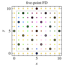
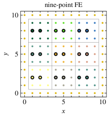
Figure 1: Splitting of $C$- and $F$- points for $11\times 11$ meshes from optimization “by hand”. At left, X-pentomino coarsening for five-point FD scheme. At right, $3\times 3$ brick coarsening for nine-point FE scheme. At left, we color by the X-pentominos and at right, we color by the $3\times 3$ bricks. $C$-points are represented by the black circles.

4 Results

In the results below, unless stated otherwise, we set the initial (global) temperature at $T=1$, and compute the reduction rate, $\alpha$, so that $\alpha^{n_{\text{ts}}}$ = 0.1, where $n_{\text{ts}}$ is the total number of annealing steps to be attempted. Thus, these experiments end when the global temperature reaches $0.1$. In addition, for each problem, we determine $n_{\text{ts}}$ by fixing a total number of steps per DoF in the system, and report results based on the allotted number of steps per DoF, $n_{\text{per DoF}}$. This work is further subdivided into Gauss-Seidel sweeps by fixing values of the number of annealing steps per DoF per sweep, $n_{\text{per DoF per cycle}}$, with the number of sweeps determined as the ratio of total steps per DoF to steps per DoF per sweep, as on 4 of Algorithm 4.

We first consider structured-grid experiments for both the finite-difference (five-point) and bilinear finite element (nine-point) discretizations of the Laplacian, using a $32\times 32$ mesh to explore how much work is needed to determine near-optimal partitions using both geometric and algebraic divisions into subdomains. Using these experiments to identify “best practices”, we then explore how the coarsening algorithm performs as we change the problem size, move from structured to unstructured finite-element meshes, and isotropic to anisotropic operators.

4.1 Structured-grid discretizations with geometrically structured subdomains

We start by considering the five-point finite-difference stencil on a fixed (uniform) $32\times 32$ mesh, and consider the effects of changing both the size of the Gauss-Seidel subdomains and the distribution of work in the algorithm. As a measure of quality of the results, we consider the maximum of the ratio $|F|/|\Omega|$ over all constraint-satisfying $F$-sets generated in a single run of the annealing algorithm. As a comparison, for this problem, the best optimization “by hand” of the size of the $F$-set yields $|F|/|\Omega|=0.8047$, as depicted by the black lines in Figure 2, while the greedy algorithm [1] yields $|F|/|\Omega|=0.561$ (not depicted because it is far from the data shown here). We vary three algorithmic parameters in Figure 2, the total number of SA steps per DoF, with values ranging from $5000$ to $2\,000\,000$, the number of SA steps per DoF in a single sweep of Gauss-Seidel on each subdomain, and the size of the subdomains used in the Gauss-Seidel sweeps.

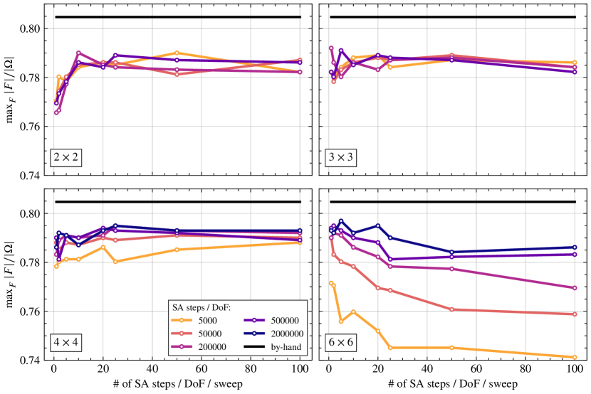
Figure 2: Maximum value of $|F|/|\Omega|$ with number of annealing steps per DoF per GS sweep for different numbers of annealing steps per DoF for the $32\times 32$ uniform-grid five-point finite-difference discretization. Each panel shows a different size of geometrically chosen subdomain: $2\times 2$ (top-left), $3\times 3$ (top-right), $4\times 4$ (bottom-left), $6\times 6$ (bottom-right).

We can draw three conclusions from the data presented in Figure 2. First, we note that if the subdomains are “too small”, then there is little benefit in investing substantial work in the SA process, as shown in the top row for $2\times 2$ and $3\times 3$ subdomains. Here, while there is clearly a small benefit to increasing the number of SA steps per DoF per sweep from 1 to about 10, there is little improvement beyond those results, and little correlation between the quality of partitioning generated and the total amount of work invested. This occurs consistently in the numerical results throughout this paper: for small subdomain sizes, each subdomain seems to have too little freedom to make adjustments into better global configurations while still satisfying local constraints. Secondly, when we consider larger subdomains (as in the bottom row), we see that doing more work overall does, indeed, pay off, particularly for the largest subdomains ($6\times 6$, at bottom right). This is also consistently observed; in particular, that for larger subdomains we see both better overall configurations (if sufficient work is performed) and improvements with larger work budgets. Finally, for the largest subdomains, we see a clear benefit to doing relatively few SA steps per DoF per cycle. Thus, in further results, we generally fix the number of SA steps per DoF per cycle to be relatively small, either 1 or 5.

A key question is how to balance the parameters in the SA algorithm to achieve reasonable performance at an acceptable cost. To examine this, we fix the total number of annealing steps per DoF and consider the best partitioning achieved by varying the subdomain size in the left panel of Figure 3. Here, we run for a number of different values of the number of SA steps per DoF per Gauss-Seidel sweep, and take the best partitioning observed over these grids for each subdomain size (noting that the optimal choice varies with subdomain size, typically being larger for small subdomain sizes and smaller for large subdomain sizes, see Table 10 in Appendix A for full details). When using $200\,000$ SA steps per DoF, there is a clear maximum in the graph for $4\times 4$ subdomains, although the relative difference in quality in not substantial; however, when using $2\,000\,000$ SA steps per DoF, we see continued improvement in the quality of the partitioning up to the $6\times 6$ subdomain case. In the right panel of Figure 3, we look more closely at the convergence of the results with increasing numbers of SA steps per DoF for the case of $6\times 6$ subdomains, again taking the best results obtained for different values of the number of SA steps per DoF per Gauss-Seidel sweep, see Table 11 in Appendix A for full details. Here, we see a clear improvement in the results up to $\mathcal{O}(10^{5})$ SA steps per DoF, and continued improvement up to $2\,000\,000$ SA steps per DoF. We recall that we fix the SA temperature reduction rate, $\alpha$, so that $\alpha\rightarrow 1$ as the number of SA steps increases, yielding the same total reduction in $T$ for each experiment. Thus, the results in Figure 3 are consistent with the expected behaviour of SA, that we can achieve results arbitrarily close to the global maximizer of our functional but only if we take many steps and slowly “cool” the SA iteration. For a more practical algorithm, we emphasize the behaviour at lower numbers of SA steps / DoF, noting that we achieve results within 5% of the best-known solution already with only $3000$ steps / DoF, and within 2% at around $50\,000$ steps / DoF.

Figure 3: Left: Change in $|F|/|\Omega|$ with subdomain size for the $32\times 32$ uniform-grid five-point finite-difference discretization, using geometric subdomains, with $5000$, $200\,000$, and $2\,000\,000$ total SA steps per DoF. Right: Change in maximum number of $F$-points with number of total SA steps per DoF for this problem using $6\times 6$ subdomains.

A natural question that arises from the right-hand panel of Figure 3 is whether the best meshes obtained occur early or late in the annealing process. That is, while we clearly see benefit from slow “cooling” of the annealing process (many SA steps per DoF), it is important to identify when the optimal results are obtained during the annealing process. Figure 4 shows the annealing history for a sample run, on the $32\times 32$ uniform grid five-point finite-difference stencil, with $2\,000\,000$ SA steps per DoF (for a total of almost $2\times 10^{9}$ annealing steps). At right, we see the temperature decay, following an exponential curve from $T=1.0$ at the first step to $T=0.1$ at the final step. At left, we plot the changes in the ratio $|F|/|\Omega|$ compared to the optimized by hand mesh for this grid (also shown). For comparison, the ratio from the greedy algorithm is also shown. We see that after an initial rapid improvement in the value of the ratio, there is a secondary period where performance improves notably but steadily, up to between $5\times 10^{8}$ and $10^{9}$ total annealing steps. This demonstrates that many annealing steps are, indeed, needed to reach the best partitioning seen here, although a good partitioning is still found after many fewer steps.

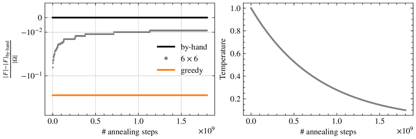
Figure 4: Change in $|F|/|\Omega|$ (left) and temperature (right) with number of annealing steps for the $32\times 32$ uniform-grid finite-difference discretization of the Laplacian. At left, the case of SA with five SA steps per DoF per GS sweep using $6\times 6$ subdomain size is shown, along with greedy as a baseline. Note that the vertical axis on the left plot uses a mixed log-linear scale for clarity, with a break at $-10^{-2}$.

Thus far, we have only considered the choice of $\alpha$ prescribed at the beginning of this section, with the decay rate chosen to yield a fixed temperature decay by a factor of 10 over the total number of SA steps given. In contrast, Figure 5 considers fixing the decay rate to be that used for $200\,000$ SA steps per DoF, $\alpha=0.1^{(1.0/(200000\times 32\times 32))}$, but then running between 4 times fewer and 2.5 times more total SA steps, with one SA step per DoF per cycle, yielding final temperature values between $0.5623$ and $0.0032$. At left of Figure 5, we observe little correlation between the total number of SA steps per DoF and the resulting value of $|F|/|\Omega|$, with all values between $0.79$ and $0.80$, comparable to those seen for similar SA budgets in Figure 3. While this appears to offer an opportunity for saving some cost in the SA algorithm (by using fewer Gauss-Seidel sweeps to get comparable results), we note that using $50\,000$ SA steps per DoF is already prohibitively expensive for an “online cost” for this algorithm, requiring more than 30 minutes to compute the partitioning for this relatively small problem.

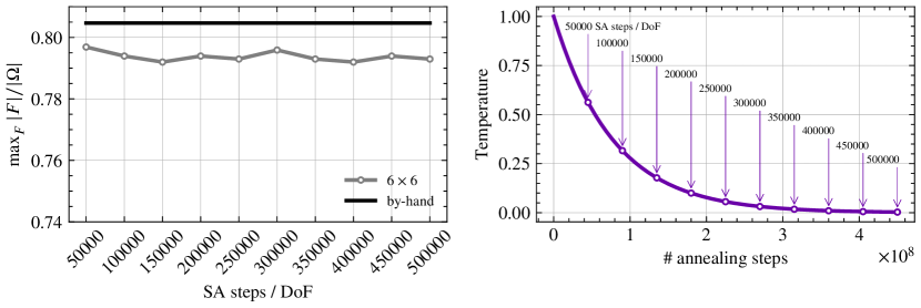
Figure 5: Change in $|F|/|\Omega|$ with SA steps per DoF for a fixed temperature decay rate (left) and temperature (right) for the $32\times 32$ uniform-grid finite-difference discretization of the Laplacian. Here, one SA step per DoF per sweep is used, and the temperature decay rate is fixed, with $\alpha=0.1^{(1.0/(200000\times 32\times 32))}$. The circles in the right figure show the stopping temperatures for the annotated SA steps per DoF.

We next address the nature of the grids generated by annealing, and whether they resemble grids that could be selected geometrically for this problem. Figure 6 shows two of the grids generated, along with the subdomains used in their generation. These represent the “best” grids found by the annealing procedure, with ratios of $|F|/|\Omega|$ of around $0.795$. While these grids yield competitive ratios, there is no clear global geometric pattern, nor obvious relationship to the best optimized by hand grid shown in Figure 1. Furthermore, there are no clear improvements of these grids that could be readily made, such as single coarse points that could be omitted without leading to constraint violations. This suggests that the energy landscape for this problem is likely dominated by locally optimal configurations that are separated by states with constraint violations and/or sharp changes in energy.

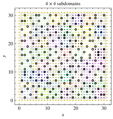
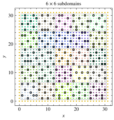
Figure 6: Grid partitioning for $32\times 32$ uniform grid with five-point FD stencil using two million SA steps per DoF. At left, the partitioning is generated using primarily $4\times 4$ subdomains, with 25 SA steps per DoF per cycle. At right, the partitioning is generated using $6\times 6$ subdomains, with 5 SA steps per DoF per cycle. The grid at left has 814 $F$-points, while that at right has 816.

Figure 7 shows how the performance of the annealing algorithm scales with problem size, for both the geometric choice of subdomains for the finite-difference discretization discussed so far, and for the finite-element discretization. In addition, an algebraic selection (discussed below) is added for comparison. All methods (including the optimization by hand) perform relatively well for small meshes, but degrade as the mesh size increases. The amount of work needed to achieve these results with the annealing algorithm also increases with grid size. For the $8\times 8$ mesh, using a single (global) subdomain, equally-good partitions to the optimization by hand can be found with just $2000$ annealing steps per DoF (and fewer when more subdomains are used). For the $16\times 16$ mesh, more work and larger subdomains are needed to achieve such performance. As noted above, with small subdomains even using $200\,000$ annealing steps per DoF does not achieve performance equal to the by-hand partitioning on the $16\times 16$ mesh. For larger subdomains, the algorithm does equal the results of the by-hand partitioning, but with increasing work as subdomain size increases: for $4\times 4$ subdomains, $10\,000$ annealing steps per DoF are needed, while $50\,000$ annealing steps per DoF are needed for $5\times 5$ subdomains. For $6\times 6$ subdomains, even using $200\,000$ annealing steps per DoF, we could not recover results matching the by-hand partitioning, although we speculate that this would have occurred with even more work invested. For larger domain sizes, the results shown in Figure 7 represent the best results found for a given grid over all runs with varying subdomain sizes, total SA steps per DoF, and SA steps per DoF per GS sweep. While these best results are, in general, achieved with the largest allocations of SA steps per DoF tried in our experiments, the marginal benefit of considering such large amounts of work to generate the coarsenings are quite low. Here, in all cases where we invested the computational effort to explore the question, we found less than a 1% improvement in $|F|/|\Omega|$ when increasing beyond $\mathcal{O}(10^{5})$ SA steps per DoF (and, in many cases, the improvement was only by one or two $F$-points).

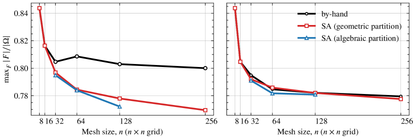
Figure 7: Change in $|F|/|\Omega|$ with mesh size for FD (left) and FE (right) discretizations.

For the nine-point finite-element stencil, we see similar results to those reported above and, consequently, do not include figures detailing the individual experiments in as much detail. Most notably, the best partitioning that we achieve by hand is a slightly worse in this case (as detailed in Section 3.4), and the partitioning using the greedy algorithm is better than in the FD case, yielding $|F|/|\Omega|=0.752$. At left of Figure 8, we show an analogous figure to Figure 2 for the case of $5\times 5$ subdomains. Here, we observe the same stratification. However, we are able to recover the same quality of partitioning as the best by-hand partitioning using $5\times 5$ subdomains and $2\,000\,000$ SA steps per DoF. Also note that we see the same mild dependence on the number of SA steps per DoF per sweep as we did in the FD case. The right panel of Figure 8 shows how the quality of partitioning changes with subdomain size and total work budget, with SA steps per DoF per sweep reported in Table 14 in Appendix A. Similarly to the FD case, there is an improvement in performance with additional work for larger subdomain sizes, but that improvement stagnates with additional work for smaller subdomain sizes. Sample grids generated for the finite-element case, including colouring to indicate subdomain choice, are shown in Figure 9.

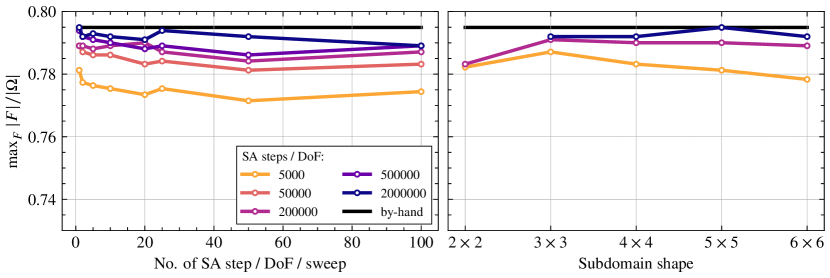
Figure 8: Quality of coarsening for the $32\times 32$ uniform-grid nine-point finite-element discretization, using geometric subdomains. Left: Maximum value of $|F|/|\Omega|$ with number of annealing steps per DoF per GS sweep for different numbers of annealing steps per DoF using $5\times 5$ geometric subdomains. Right: Change in $|F|/|\Omega|$ with subdomain size and total number of SA steps per DoF.

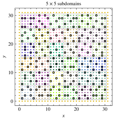
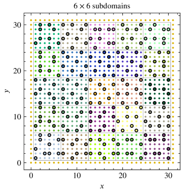
Figure 9: Grid partitioning for $32\times 32$ uniform grid with nine-point FE stencil using two million SA steps per DoF. At left, the partitioning is generated using $5\times 5$ subdomains, with one SA step per DoF per cycle. At right, the partitioning is generated using $6\times 6$ subdomains, also with one SA step per DoF per cycle. The grid at left has 814 $F$-points, while that at right has 811.

Finally, we verify that the result two-level AMGr algorithms are at least as effective as predicted in theory, by measuring asymptotic convergence factors ($\rho$), grid complexities ($C_{\text{grid}}$, equal to the ratio of sum of the number of DoFs on each level of the hierarchy to that on the finest level), and operator complexities ($C_{\text{op}}$, equal to the ratio of the sum of the number of nonzero entries in the system matrix on each level of the hierarchy to that on the finest level). We approximate $\rho$ by running the cycle with a random initial guess, $x^{(0)}$, and zero right-hand side, and then compute $\left(\left\|x^{(k)}\right\|/\left\|x^{(0)}\right\|\right)^{1/k}$, where $x^{(k)}$ is the approximation (to the true solution, which is the zero vector) after $k$ cycles. Because the convergence factors of AMGr are somewhat larger than those for classical AMG, we take $k=800$ to ensure that we sample the asymptotic behaviour suitably. Table 1 reports this data for two-level cycles for both the FD and FE discretizations, for both the geometric subdomain choice considered here and the algebraic subdomain choice discussed next. Considering the geometric subdomain choice, we see grid-independent convergence factors of about 0.9 for the FD case and 0.7 for the FE case. While these are notably worse than are observed for typical multigrid methods for these problems, they are consistent with the existing results for AMGr and, in particular, conform with the convergence rate bound from Theorem 2.1 of 0.977 for $\theta=0.56$ and $\nu=1$. Notably, neither the convergence factor nor the measured complexities degrade substantially with problem size. We note that, in subsequent work, we have improved convergence of AMGr for these and other model problems [41].

Table 1: Performance of two-level AMGr on test matrices from discretizations of the 2D Laplacian.

		Geometric Subdomains			Algebraic Subdomains
Scheme	Grid size	$\rho$	$C_{\text{grid}}$	$C_{\text{op}}$	$\rho$	$C_{\text{grid}}$	$C_{\text{op}}$
	$8\times 8$	0.85	1.16	1.12	0.85	1.16	1.12
	$16\times 16$	0.86	1.19	1.18	0.86	1.19	1.18
FD	$32\times 32$	0.88	1.20	1.20	0.88	1.21	1.20
	$64\times 64$	0.89	1.22	1.22	0.88	1.22	1.22
	$128\times 128$	0.89	1.22	1.23	0.88	1.22	1.23
	$8\times 8$	0.70	1.16	1.15	0.70	1.16	1.15
	$16\times 16$	0.63	1.20	1.22	0.63	1.20	1.22
FE	$32\times 32$	0.67	1.21	1.23	0.69	1.21	1.25
	$64\times 64$	0.71	1.21	1.25	0.72	1.22	1.27
	$128\times 128$	0.71	1.22	1.27	0.71	1.22	1.27

4.2 Structured-grid discretizations with algebraically chosen subdomains

We next consider partitioning the structured-grid problems using an algebraic choice of the subdomains based on Lloyd aggregation. Figure 10 shows the change in the maximum number of $F$-points (scaled by the total number of DoFs) with the change of the subdomain size for both the FD and FE discretizations (left and right, respectively). Similarly to the case of geometric partitioning, we see relatively poor performance for small subdomain sizes, regardless of the work allocated to the SA process. For larger subdomain sizes, we see improving results with number of SA steps per DoF, as seen above. Also as seen above, the optimal subdomain size varies with total work allocation, increasing as we increase the amount of work per DoF, but even with $2\,000\,000$ SA steps per DoF, we do not see the best performance with largest subdomains for the FE discretization. Considering variation in problem size, Figure 7 shows that, as in the geometric subdomain case, we see some decrease in performance as problem size grows, but that this decrease seems to (mostly) plateau at larger problem sizes. In comparison with the geometric subdomain choice, we see some small degradation in performance with algebraically chosen subdomains, particularly in the FD case, but it is small in comparison with the optimality gap between the optimization by hand solutions and those generated by SA.

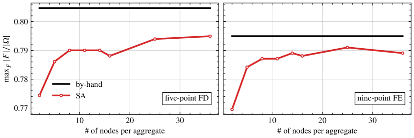
Figure 10: Change in maximum number of $F$-points with subdomain size for algebraic subdomain selection on $32\times 32$ meshes. Left and right figures are for FD and FE schemes, respectively, showing the largest value of $|F|/|\Omega|$ attained over experiments with fixed subdomain size and varying the total number of SA steps per DoF and SA steps per sweep, as in the geometric subdomain case.

Performance of the resulting two-grid cycles is tabulated in Table 1, where we see very comparable convergence factors, as well as grid and operator complexities, as in the geometric subdomain case. Table 2 tabulates convergence factors for three-level V- and W-cycles (denoted $\rho_{V}$ and $\rho_{W}$, respectively), along with three-level grid and operator complexities. For the FD case, we see some degradation in convergence when using V-cycles, while W-cycles give convergence factors similar to those in the two-level case. For the FE problem, there is less degradation for V-cycles, but still W-cycles are required to get convergence factors comparable to the two-level case. As we have increased the depth of the multigrid hierarchy, the grid and operator complexities in Table 2 are naturally larger than those in Table 1, but the growth in these complexity measures is consistent with optimally scaling multigrid methods. Performance of multilevel V- and W-cycles is also shown in Table 2, where coarsening is continued until the number of nodes falls below $100$, yielding a four-level cycle for the $32\times 32$ grid, five-level cycle for $64\times 64$, and six-level cycle for $128\times 128$. The resulting convergence factors for both FD and FE cases remain similar to those for three-level cycles, while complexity measures grow consistently with the number of levels.

Table 2: Performance of three-level and multilevel AMGr on test matrices from discretizations of the 2D Laplacian.

		Three-level cycles				Multilevel cycles
Scheme	Grid size	$\rho_{V}$	$\rho_{W}$	$C_{\text{grid}}$	$C_{\text{op}}$	$\rho_{V}$	$\rho_{W}$	$C_{\text{grid}}$	$C_{\text{op}}$
	$32\times 32$	0.92	0.90	1.25	1.26	0.93	0.90	1.26	1.27
FD	$64\times 64$	0.93	0.91	1.27	1.28	0.94	0.91	1.28	1.31
	$128\times 128$	0.94	0.91	1.28	1.30	0.95	0.92	1.30	1.35
	$32\times 32$	0.76	0.72	1.25	1.31	0.76	0.72	1.26	1.31
FE	$64\times 64$	0.76	0.73	1.27	1.35	0.77	0.73	1.28	1.37
	$128\times 128$	0.79	0.75	1.28	1.37	0.79	0.75	1.29	1.41

For the multilevel results in Table 2, we use $200\,000$ SA steps per DoF in all cases, except on the finest meshes for the $32\times 32$ and $64\times 64$ grids, where $2\,000\,000$ SA steps per DoF were used. (Similar results are also seen without these “extra” steps on these problems, however.) For the $64\times 64$ mesh, using $200\,000$ SA steps per DoF on all levels takes about 18 hours of “offline” time to compute the coarse meshes, in comparison to “online” solution times of only 0.003 seconds for a V-cycle and 0.011 seconds for a W-cycle. Table 3 presents results for the same experiment, but using only $200$ and $2000$ SA steps per DoF, to investigate how performance is changed when using “bad” solutions to the optimization problem in Equation 3. Here, we see slight improvements in convergence factors in comparison to those in Table 2; however, using fewer annealing steps leads to much larger grid and operator complexities than observed above. We note here that using fewer annealing steps also leads to results that are more heavily influenced by the random nature of the SA process; here, we report complexities from runs used to generate W-cycle convergence factors, which vary slightly from those of an independent run to generate V-cycle convergence factors, but by no more than $0.01$ in $C_{\text{grid}}$ and $0.05$ in $C_{\text{op}}$.

Table 3: Performance of multilevel AMGr on test matrices from discretizations of the 2D Laplacian using $200$ and $2000$ SA steps per DoF.

		$200$ SA steps per DoF				$2000$ SA steps per DoF
Scheme	Grid size	$\rho_{V}$	$\rho_{W}$	$C_{\text{grid}}$	$C_{\text{op}}$	$\rho_{V}$	$\rho_{W}$	$C_{\text{grid}}$	$C_{\text{op}}$
	$32\times 32$	0.89	0.86	1.42	1.62	0.91	0.88	1.33	1.44
FD	$64\times 64$	0.89	0.88	1.46	1.86	0.92	0.88	1.37	1.51
	$128\times 128$	0.91	0.88	1.48	2.08	0.93	0.89	1.38	1.58
	$32\times 32$	0.72	0.68	1.34	1.52	0.73	0.71	1.29	1.40
FE	$64\times 64$	0.74	0.70	1.37	1.65	0.76	0.70	1.32	1.49
	$128\times 128$	0.77	0.70	1.38	1.76	0.76	0.72	1.33	1.56

For our final isotropic, structured-grid test problem, we consider the FE discretization of the two-dimensional isotropic diffusion problem, $-\nabla\cdot\boldsymbol{K}(x,y)\nabla u(x,y)=f(x,y)$, in the domain $[0,1]\times[0,1]$ with Dirichlet boundary conditions and piecewise constant (“jumping”) coefficient, $\boldsymbol{K}(x,y)$. To determine $\boldsymbol{K}(x,y)$, we select 20% of the elements at random, and set $\boldsymbol{K}(x,y)=10^{-8}$ in these elements, with value $1$ in the remaining 80% of the elements, matching one of the test problems from [1]. We partition the nodes using $200\,000$ SA steps per DoF, and show the first coarse mesh chosen using $1$ SA step per DoF per sweep for the $31\times 31$ grid in Figure 11. Convergence factors and grid and operator complexities for multilevel V- and W-cycles are shown in Table 4. We note, in particular, that these results are quite comparable to those shown in Table 2 for the case of $\boldsymbol{K}(x,y)=1$ everywhere. In comparison to the results presented in [1], we see larger convergence factors here (0.78 for the $127\times 127$ grid, in comparison to 0.59 reported there), but with lower complexities ($C_{\text{op}}=1.42$ here, compared to $1.75$ there).

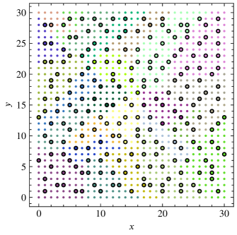
Figure 11: Partitioning for the isotropic problem on a $31\times 31$ uniform grid with jumping coefficients, generated using $200\,000$ SA steps per DoF, 1 SA step per DoF per GS sweep, and subdomains with an average of 36 points per subdomain. $C$-points are represented by the black circles.

Table 4: Performance of multilevel AMGr on test matrices from discretizations of the 2D Laplacian with jumping coefficients.

Scheme	Grid size	$\rho_{V}$	$\rho_{W}$	$C_{\text{grid}}$	$C_{\text{op}}$
	$31\times 31$	0.73	0.71	1.27	1.33
FE	$63\times 63$	0.76	0.73	1.29	1.38
	$127\times 127$	0.78	0.76	1.29	1.42

4.3 Anisotropic problems on structured grids

Next, we consider the two-dimensional anisotropic diffusion problem, $-\nabla\cdot\boldsymbol{K}(x,y)\nabla u(x,y)=f(x,y)$, in the domain $[0,1]\times[0,1]$ with Dirichlet boundary conditions. We choose the tensor coefficient $\boldsymbol{K}(x,y)=QMQ^{T}$, where $Q=\begin{bmatrix}\cos(\theta)&-\sin(\theta)\\ \sin(\theta)&\cos(\theta)\end{bmatrix}$, and $M=\begin{bmatrix}\delta&0\\ 0&1\end{bmatrix}$. The parameters $0<\delta\leq 1$ and $\theta$ specify the strength and direction of anisotropy in the problem, respectively, with $\theta=0$ giving the anisotropic problem $-\delta u_{xx}-u_{yy}=f$ and $\theta=\pi/2$ giving $-u_{xx}-\delta u_{yy}=f$. For $0<\theta<\pi/2$, the axis of the small diffusion coefficient in the problem rotates clockwise from being in the positive $x$-direction for small $\theta$ to the positive $y$-direction for $\theta\approx\pi/2$. Anisotropic problems cause difficulty for the greedy coarsening algorithm [1], where large grid and operator complexities and poor algorithmic performance were overcome by augmenting the coarse grids with the second pass of the Ruge-Stüben coarsening algorithm and using classical AMG interpolation in place of the AMGr interpolation operator. We emphasize that both the FD and FE discretizations of this problem result in non-diagonally dominant system matrices and, consequently, the convergence guarantee from Theorem 2.1 does not apply in this setting. We include these problems, nonetheless, both to stress-test our approach and highlight the need for further research in this direction.

As an example of a problem in this class, we fix $\delta=10^{-6}$ and $\theta=\pi/3$. Figure 12 shows the coarse-grid points selected for the bilinear finite-element discretization of the problem on a uniform $32\times 32$ mesh. At left, we see that the partitioning generated by the SA algorithm correctly detects that this is an anisotropic problem with strong coupling primarily in the $x$-direction and weak coupling primarily in the $y$-direction, producing grids that are consistent with semi-coarsening, with some regions of coarsening along diagonals. Unfortunately, however, this grid leads to poor convergence using AMGr interpolation. As in the original experiments by MacLachlan and Saad [1], each fine-grid point has multiple coarse-grid neighbours (leading to an increase in operator complexity, due to the nonzero structure of $D_{FF}^{-1}A_{FC}$), but since $A$ is no longer diagonally dominant in the anisotropic case, the assumption that $\begin{bmatrix}D_{FF}&-A_{FC}\\ -A_{FC}^{T}&A_{CC}\end{bmatrix}$ is positive semi-definite is violated, and the resulting performance is poor. To overcome this failure, we augment the coarse-grid set using the second-pass algorithm from Ruge-Stüben AMG, using the classical strength of connection parameter of $0.30$ to determine strong connections in the graph. At right of Figure 12, we show the resulting graph, which now satisfies the requirement that every pair of strongly connected $F$-points has a common $C$-neighbour (which is clearly not satisfied in the partitioning at left). Unfortunately, this comes at a heavy cost, as the grid at right now has many more $C$-points than we would like. Below, we verify that these grids lead to effective multigrid hierarchies, when coupled with classical AMG interpolation, but note the increased grid and operator complexities in these hierarchies. A key question for future work (addressed in [41]) is whether we can determine algebraic interpolation operators for grids such as those at left that lead to effective AMGr performance.

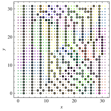
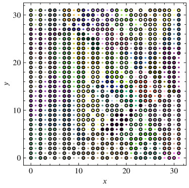
Figure 12: Grid partitioning for an anisotropic diffusion problem with $\delta=10^{-6}$ and $\theta=\pi/3$, discretized on a $32\times 32$ mesh using the bilinear FE stencil. The initial partitioning, at left, is generated using algebraic subdomains averaging 20 points per subdomain, using $2\,000\,000$ SA steps per DoF and 1 SA step per DoF per GS sweep, and has 664 $F$-points and 360 $C$-points. At right is the grid augmented using the second pass of the classical AMG algorithm, resulting in 343 $F$-points and 681 $C$-points.

Tables 5 and 6 present convergence factors and grid and operator complexities for two- and three-level cycles, respectively. For geometric partitioning, we use $200\,000$ SA steps per DoF with one or two SA steps per DoF per cycle and $5\times 5$ or $6\times 6$ subdomains (depending on what worked best for a given problem, reported in Table 16 in Appendix A). Similar choices are made using algebraic partitioning, although we see slight improvements using $2\,000\,000$ SA steps per DoF for some problems. For the three-level tests, we uniformly use $200\,000$ SA steps per DoF, with 1 SA step per DoF per GS sweep, and algebraic subdomains with average size of 36 points. In Table 5, we again see that there is relatively little difference in results generated using geometric and algebraic choices of the Gauss-Seidel subdomains. Notably, both choices lead to effective cycles for both the finite-difference and finite-element discretizations, albeit at the cost of increased grid and operator complexities. Table 6 again shows degradation in performance moving from two-grid to three-grid V-cycles, but that three-grid W-cycles mostly recover comparable convergence to the two-level case, with some notable degradation for the finite-element operator.

Table 5: Performance of two-level AMGr for the anisotropic diffusion problem with $\delta=10^{-6}$ and $\theta=\pi/3$ on structured meshes.

		Geometric Partitioning			Algebraic Partitioning
Scheme	Grid size	$\rho$	$C_{\text{grid}}$	$C_{\text{op}}$	$\rho$	$C_{\text{grid}}$	$C_{\text{op}}$
	$32\times 32$	0.58	1.70	2.09	0.57	1.70	2.09
FD	$64\times 64$	0.58	1.71	2.11	0.58	1.71	2.11
	$128\times 128$	0.60	1.72	2.12	0.63	1.72	2.12
	$32\times 32$	0.62	1.65	2.02	0.61	1.67	2.00
FE	$64\times 64$	0.61	1.67	2.09	0.62	1.67	2.08
	$128\times 128$	0.61	1.67	2.11	0.61	1.67	2.12

Table 6: Performance of three-level AMGr for the anisotropic diffusion problem with $\delta=10^{-6}$ and $\theta=\pi/3$ on structured meshes.

Scheme	Grid size	$\rho_{V}$	$\rho_{W}$	$C_{\text{grid}}$	$C_{\text{op}}$
	$32\times 32$	0.72	0.57	2.16	3.13
FD	$64\times 64$	0.76	0.60	2.16	3.20
	$128\times 128$	0.80	0.66	2.18	3.26
	$32\times 32$	0.74	0.61	2.06	2.86
FE	$64\times 64$	0.81	0.69	2.07	3.05
	$128\times 128$	0.89	0.82	2.05	3.10

4.4 Discretizations on unstructured grids

We next consider two diffusion problems with homogeneous Dirichlet boundary conditions on unstructured triangulations of square domains, discretized using linear finite elements. First, we consider an isotropic diffusion operator ($-\nabla\cdot\nabla u=f$) on $[-1,1]^{2}$, generated by taking an initially unstructured mesh, refining it a set number of times and, then, smoothing the resulting mesh. We consider three levels of refinement for this example, resulting in meshes with $1433$, $5617$, and $22\,241$ DoFs. The SA-based partitioning scheme appears to perform similarly well in this setting, with a splitting found for the smallest mesh shown in Figure 13. While we no longer have hand-generated estimates of the optimal coarsening factors, we note that the SA-based partitioning scheme outperforms the greedy algorithm, generating $F$-sets with $1106$, $4241$, and $16\,604$ points, for these three grids, respectively, in comparison to $F$-sets of $1024$, $3916$, and $15\,079$ points. As above, this improvement comes at a cost: the offline time to partition the $5617$ DoF problem using $200\,000$ SA steps per DoF is over 12 hours for the two-level scheme. Two- and three-level convergence factors, as well as grid and operator complexities for these systems are given in Table 7. Here, we observe that these results are quite similar to those seen for the structured-grid discretizations above, with some degradation in convergence seen for the three-level V-cycle results, but not in the W-cycle results. Here, the three-level results are computed using $200\,000$ SA steps per DoF, with 1 SA step per DoF per GS sweep, on subdomains with an average of 36 points per subdomain. Slight modifications to these parameters yield small improvements in two-level results; as a result, we use these choices in the table and report them in Table 17 in Appendix A.

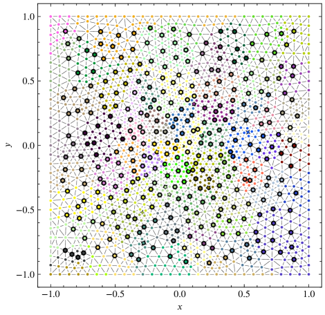
Figure 13: Partitioning for the isotropic problem on the unstructured mesh with $1433$ points, generated using $1\,000\,000$ SA steps per DoF, 5 SA steps per DoF per GS sweep, and subdomains with an average of 20 points per subdomain.

Table 7: Performance of two- and three-level AMGr for isotropic problem on unstructured meshes.

	Two-level cycle			Three-level cycles
#DoF	$\rho$	$C_{\text{grid}}$	$C_{\text{op}}$	$\rho_{V}$	$\rho_{W}$	$C_{\text{grid}}$	$C_{\text{op}}$
1433	0.66	1.23	1.31	0.78	0.65	1.28	1.39
5617	0.71	1.25	1.32	0.79	0.70	1.30	1.42
22241	0.75	1.25	1.33	0.84	0.75	1.32	1.45

We next consider the anisotropic diffusion operator (again with Dirichlet boundary conditions) considered above, with $\delta=0.01$ and $\theta=\pi/3$, on an unstructured triangulation of the unit square taken from Brannick and Falgout [23], matching the problem labelled 2D-M2-RLap in that paper. As in Brannick and Falgout [23], we consider three levels of refinement of the mesh, with $798$, $3109$, and $12\,273$ DoFs, respectively. Figure 14 shows two different partitions for this mesh. At left, we give the partitioning generated using the SA-based partitioning algorithm proposed here, and at right we give the splitting after a second pass of the Ruge-Stüben coarsening algorithm where strength of connection is computed using the classical strength parameter of $0.55$. As with the structured-grid case above, we found the second pass is needed to achieve good convergence factors for the anisotropic problem, but that it does so at the expense of coarsening at a much slower rate. Convergence factors, grid complexities, and operator complexities for these problems are reported in Table 8. As above, the complexities are higher for the anisotropic operators than the isotropic (due to the use of the second pass). Here, we observe degradation in convergence with grid refinement, although again with less degradation for W-cycles than V-cycles. The three-level results are computed with the same parameters as for the isotropic problem above, with more SA steps per DoF used for the two-level results, as this yielded slight improvements. While the performance reported in Table 8 is far from optimal, we note that the convergence factors for the larger two meshes are better than those reported for compatible relaxation [23], while the operator complexities are comparable to those reported therein for BoomerAMG [5]. We again emphasize that these anisotropic diffusion problems do not satisfy the convergence bounds stated above and, consequently, are included to stress-test the framework presented here; improved results for this problem are presented in [41].

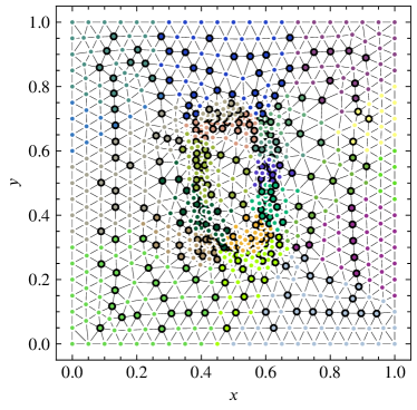
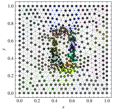
Figure 14: Partitioning for the anisotropic problem on an unstructured mesh containing 798 points. The partitioning at left was generated using $500\,000$ SA steps per DoF, with 1 SA step per DoF per GS sweep, on subdomains with an average size of 36 points per subdomain, yielding 524 $F$-points and 274 $C$-points. At right, this partitioning is augmented by the second pass of classical AMG coarsening, resulting in 263 $F$-points and 535 $C$-points.

Table 8: Performance of two-level and three-level AMGr for anisotropic problem on unstructured meshes.

	Two-level cycle			Three-level cycles
#DoF	$\rho$	$C_{\text{grid}}$	$C_{\text{op}}$	$\rho_{V}$	$\rho_{W}$	$C_{\text{grid}}$	$C_{\text{op}}$
798	0.69	1.67	1.82	0.84	0.71	2.11	2.41
3109	0.75	1.67	1.87	0.84	0.75	2.09	2.52
12273	0.82	1.67	1.89	0.90	0.83	2.08	2.56

4.5 Convection-diffusion problems on structured grids

For our final tests, we consider the upwind finite-difference discretization of two singularly perturbed convection-diffusion equations. While these problems lead to non-symmetric discretization matrices (and, as such, Theorem 2.1 no longer applies), they represent a plausible set of test problems for reduction-based methods due to their “nearly triangular” M-matrix structure [31]. In particular, we consider the solution of the convection-diffusion equation,

$$-\varepsilon\Delta u+\boldsymbol{b}\cdot\nabla u=f,$$

with homogeneous Dirichlet boundary conditions, for two choices of the convection direction:

grid-aligned convection $$\boldsymbol{b}=\begin{bmatrix}1\\ 0\end{bmatrix},$$

non-grid-aligned convection $$\boldsymbol{b}=\begin{bmatrix}2\\ 3\end{bmatrix}.$$

We discretize these problems on uniform $N\times N$ meshes with the standard 5-point finite-difference for the diffusion term, and a first-order upwind finite-difference discretization for the convection terms. In all experiments, we use $200\,000$ SA steps per DoF to generate the partitioning, and generate the AMGr interpolation operator by computing $\begin{bmatrix}D_{FF}^{-1}A_{FC}\\ I\end{bmatrix}$. We construct the restriction operator by taking $\begin{bmatrix}A_{CF}D_{FF}^{-1}&I\end{bmatrix}$. Table 9 reports measured asymptotic convergence factors, along with grid and operator complexities for these problems, showing insensitivity to both problem size and the singular perturbation parameter, $\varepsilon$. Figure 15 shows two sample partitioning, one for each convection direction, illustrated at $\varepsilon=10^{-5}$ for $N=32$.

Table 9: Performance of two-level AMGr for convection-diffusion problems on structured meshes.

		Grid-Aligned			Non-Grid-Aligned
$\varepsilon$	$N$	$\rho$	$C_{\text{grid}}$	$C_{\text{op}}$	$\rho$	$C_{\text{grid}}$	$C_{\text{op}}$
	16	0.617	1.50	1.93	0.617	1.34	1.65
$10^{-3}$	32	0.617	1.50	2.01	0.617	1.36	1.71
	64	0.617	1.51	2.02	0.617	1.36	1.74
	16	0.617	1.50	1.93	0.617	1.34	1.63
$10^{-4}$	32	0.617	1.50	1.97	0.617	1.36	1.71
	64	0.617	1.51	2.03	0.617	1.36	1.74
	16	0.617	1.50	1.92	0.617	1.33	1.63
$10^{-5}$	32	0.617	1.51	2.00	0.617	1.36	1.71
	64	0.617	1.51	2.03	0.617	1.36	1.73

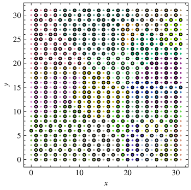
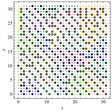
Figure 15: Partitioning for convection-diffusion problems on uniform grids, for the grid-aligned case, at left, and the non-grid-aligned case, at right. In both cases, we depict the partitioning for $\varepsilon=10^{-5}$ and $N=32$, generated using $200\,000$ SA steps per DoF.

5 Conclusions and future work

While existing heuristics for coarse-grid selection within AMG offer reliable performance for a wide class of problems, there remains much interest in both improving our understanding of AMG convergence and developing new approaches that offer guarantees of convergence for even wider classes of problems. We believe a promising, yet under-explored, area of research is in the extension of reduction-based AMG approaches, that have been shown to be effective for both isotropic diffusion problems [26, 1] and more interesting classes of problems, such as some hyperbolic PDEs [31]. In this paper, we propose a new coarsening algorithm for AMGr, based on applying simulated annealing to the optimization problem first posed by MacLachlan and Saad [1]. We choose SA as it is a widely used optimization technique that can be applied to combinatorial optimization problems. Other techniques are certainly possible (e.g., genetic algorithms or particle swarm optimization), and it may be that those techniques lead to improved performance. For isotropic problems on both structured and unstructured meshes, we find that the SA-based partitioning approach outperforms the original greedy algorithm, sometimes dramatically, while sharing some of the existing limitations of the AMGr framework, particularly for anisotropic problems. We believe that the performance difference between the greedy and SA-based algorithm is, simply, due to the complex nature of the optimization problem at hand. The greedy algorithm makes the best “local” choice at each stage, but those local choices force poor global configurations. In particular, the greedy approach has no opportunity to undo a choice already made, while the SA approach allows that to happen. Nonetheless, we see this as an important proof-of-concept, showing that randomized search and other derivative-free optimization algorithms can be successfully applied to the combinatorial optimization problems in AMG coarsening.

The main drawback of this approach is the high computational cost of simulated annealing. For example, computing a single coarse grid for a $32\times 32$ mesh with $200\,000$ SA steps per DoF required around 2.5 hours on a modern workstation, primarily for evaluating the fitness functional in the optimization, with expected scaling in problem size and number of SA steps per DoF. Two key questions that this raises are whether the fitness functional can be approximated in a more efficient manner (e.g., using a value neural network) and whether other optimization techniques that rely on fewer samplings of the fitness functional can be applied. Both of these are topics of our current research.

This research also exposes a known weakness of the AMGr methodology (and, to our knowledge, one of all AMG-like algorithms with guarantees on convergence rates) when applied to problems that are not diagonally dominant (such as finite-element discretization of anisotropic diffusion equations). Another current research direction is identifying whether the diagonal choice of $D_{FF}$ can be generalized to yield better convergence (while retaining a guaranteed convergence rate), and whether such changes can be accommodated within the optimization problems solved here. Preliminary results in this direction are presented in [41].

Appendix A Additional Data

In this section, we provide some additional tables to provide more complete data on the experiments reported above.

SA steps / DoF	$2\times 2$	$3\times 3$	$4\times 4$	$5\times 5$	$6\times 6$
$5000$	50	20	100	2	1
$200\,000$	10	1	25	5	2
$2\,000\,000$	–	–	25	20	5

Table 10: Number of SA steps per DoF per sweep used for numerical results in left-hand panel of Figure 3.

SA steps / DoF:	$3000$	$5000$	$7500$	$10\,000$	$50\,000$	$100\,000$	$200\,000$	$500\,000$	$2\,000\,000$
SA steps / DoF / cycle:	1	1	1	2	1	2	2	2	5

Table 11: Number of SA steps per DoF per sweep used for numerical results in right-hand panel of Figure 3.

Partitioning		FD Discretization
		$8\times 8$	$16\times 16$	$32\times 32$	$64\times 64$	$128\times 128$	$256\times 256$
	SA steps per DoF	$1000$	$10\,000$	$2\,000\,000$	$2\,000\,000$	$200\,000$	$200\,000$
Geometric	SA steps per DoF per cycle	1	100	5	1	1	1
	Subdomain size	$2\times 2$	$4\times 4$	$6\times 6$	$6\times 6$	$6\times 6$	$6\times 6$
	SA steps per DoF	–	–	$2\,000\,000$	$2\,000\,000$	$200\,000$	–
Algebraic	SA steps per DoF per cycle	–	–	2	1	1	–
	Subdomain size	–	–	36	36	36	–

Table 12: Number of SA steps and SA steps per DoF per sweep used for numerical results in left-hand panel of Figure 7.

Partitioning		FE Discretization
		$8\times 8$	$16\times 16$	$32\times 32$	$64\times 64$	$128\times 128$	$256\times 256$
	SA steps per DoF	$1000$	$200\,000$	$2\,000\,000$	$1\,000\,000$	$200\,000$	$200\,000$
Geometric	SA steps per DoF per cycle	25	25	50	100	1	1
	Subdomain size	$2\times 2$	$3\times 3$	$4\times 4$	$3\times 3$	$5\times 5$	$5\times 5$
	SA steps per DoF	–	–	$2\,000\,000$	$200\,000$	$2\,000\,000$	–
Algebraic	SA steps per DoF per cycle	–	–	1	1	1	–
	Subdomain size	–	–	25	25	25	–

Table 13: Number of SA steps and SA steps per DoF per sweep used for numerical results in right-hand panel of Figure 7.

SA steps / DoF	$2\times 2$	$3\times 3$	$4\times 4$	$5\times 5$	$6\times 6$
$5000$	20	10	5	1	1
$200\,000$	10	2	50	20	2
$2\,000\,000$	–	–	50	1	1

Table 14: Number of SA steps per DoF per sweep used for numerical results in right-hand panel of Figure 8.

$\#$ of nodes per aggregate	2	5	8	11	14	16	25	36
FD:
SA steps per DoF	$200\,000$	$7500$	$100\,000$	$200\,000$	$200\,000$	$1\,000\,000$	$500\,000$	$2\,000\,000$
SA steps per DoF per cycle	10	10	20	5	50	25	1	2
FE:
SA steps per DoF	$7500$	$200\,000$	$2\,000\,000$	$200\,000$	$200\,000$	$200\,000$	$2\,000\,000$	$2\,000\,000$
SA steps per DoF per cycle	5	100	20	50	1	1	1	1

Table 15: Number of SA steps and SA steps per DoF per sweep used for numerical results in Figure 10.

Partitioning		FD Discretization			FE Discretization
		$32\times 32$	$64\times 64$	$128\times 128$	$32\times 32$	$64\times 64$	$128\times 128$
	SA steps per DoF	$200\,000$	$200\,000$	$200\,000$	$200\,000$	$200\,000$	$200\,000$
Geometric	SA steps per DoF per cycle	1	1	1	2	1	1
	Subdomain size	$6\times 6$	$6\times 6$	$6\times 6$	$5\times 5$	$5\times 5$	$5\times 5$
	SA steps per DoF	$200\,000$	$200\,000$	$200\,000$	$2\,000\,000$	$200\,000$	$2\,000\,000$
Algebraic	SA steps per DoF per cycle	1	1	1	1	1	2
	Subdomain size	16	36	36	20	36	36

Table 16: Number of SA steps per DoF and SA steps per DoF per sweep and subdomain sizes used for two-level numerical results in Table 5.

	Table 7			Table 8
	1433	5617	22241	798	3109	12273
SA steps per DoF	$1\,000\,000$	$2\,000\,000$	$200\,000$	$500\,000$	$2\,000\,000$	$200\,000$
SA steps per DoF per cycle	5	2	1	1	2	1
Subdomain size	20	36	36	36	36	36

Table 17: Number of SA steps per DoF and SA steps per DoF per sweep and subdomain sizes used for two-level numerical results in Tables 7 and 8.

References

- MacLachlan and Saad [2007] S. MacLachlan, Y. Saad, A greedy strategy for coarse-grid selection, SIAM Journal on Scientific Computing 29 (2007) 1825–1853. doi:10.1137/060654062.
- Brandt et al. [1982] A. Brandt, S. F. McCormick, J. W. Ruge, Algebraic multigrid (AMG) for automatic multigrid solutions with application to geodetic computations, Technical Report, Inst. for Computational Studies, Fort Collins, Colo., 1982.
- Brandt et al. [1984] A. Brandt, S. F. McCormick, J. W. Ruge, Algebraic multigrid (AMG) for sparse matrix equations, in: D. J. Evans (Ed.), Sparsity and Its Applications, Cambridge University Press, Cambridge, 1984, pp. 257–284.
- Falgout and Yang [2002] R. Falgout, U. Yang, Hypre: A library of high performance preconditioners, in: Computational Science - ICCS 2002: International Conference, Amsterdam, The Netherlands, April 21-24, 2002. Proceedings, Part III, volume 2331 of Lecture Notes in Computer Science, Springer-Verlag, 2002, pp. 632–641.
- Henson and Yang [2002] V. Henson, U. Yang, BoomerAMG: A parallel algebraic multigrid solver and preconditioner, Applied Numerical Mathematics 41 (2002) 155–177.
- Balay et al. [2008] S. Balay, K. Buschelman, V. Eijkhout, W. D. Gropp, D. Kaushik, M. G. Knepley, L. C. McInnes, B. F. Smith, H. Zhang, PETSc Users Manual, Technical Report ANL-95/11 - Revision 3.0.0, Argonne National Laboratory, 2008.
- Balay et al. [2010] S. Balay, K. Buschelman, W. D. Gropp, D. Kaushik, M. G. Knepley, L. C. McInnes, B. F. Smith, H. Zhang, PETSc Web page, Technical Report, 2010. Http://www.mcs.anl.gov/petsc.
- Heroux et al. [2005] M. A. Heroux, R. A. Bartlett, V. E. Howle, R. J. Hoekstra, J. J. Hu, T. G. Kolda, R. B. Lehoucq, K. R. Long, R. P. Pawlowski, E. T. Phipps, A. G. Salinger, H. K. Thornquist, R. S. Tuminaro, J. M. Willenbring, A. Williams, K. S. Stanley, An overview of the Trilinos project, ACM Trans. Math. Softw. 31 (2005) 397–423. doi:http://doi.acm.org/10.1145/1089014.1089021.
- Gee et al. [2006] M. Gee, C. Siefert, J. Hu, R. Tuminaro, M. Sala, ML 5.0 Smoothed Aggregation User’s Guide, Technical Report SAND2006-2649, Sandia National Laboratories, 2006.
- Olson and Schroder [2018] L. N. Olson, J. B. Schroder, PyAMG: Algebraic Multigrid Solvers in Python v4.0, Technical Report, 2018. URL: https://github.com/pyamg/pyamg, release 4.0.
- Vaněk et al. [1996] P. Vaněk, J. Mandel, M. Brezina, Algebraic multigrid by smoothed aggregation for second and fourth order elliptic problems, Computing 56 (1996) 179–196.
- Stüben [2001] K. Stüben, An introduction to algebraic multigrid, in: U. Trottenberg, C. Oosterlee, A. Schüller (Eds.), Multigrid, Academic Press, London, 2001, pp. 413–528.
- Ruge and Stüben [1987] J. W. Ruge, K. Stüben, Algebraic multigrid (AMG), in: S. F. McCormick (Ed.), Multigrid Methods, volume 3 of Frontiers in Applied Mathematics, SIAM, Philadelphia, PA, 1987, pp. 73–130.
- Alber and Olson [2007] D. M. Alber, L. N. Olson, Parallel coarse-grid selection, Numerical Linear Algebra with Applications 14 (2007) 611–643. URL: http://dx.doi.org/10.1002/nla.541.
- Cleary et al. [1998] A. J. Cleary, R. D. Falgout, V. E. Henson, J. E. Jones, Coarse-grid selection for parallel algebraic multigrid, in: Proc. of the Fifth International Symposium on Solving Irregularly Structured Problems in Parallel, volume 1457 of Lecture Notes in Computer Science, Springer–Verlag, New York, 1998, pp. 104–115.
- De Sterck et al. [2006] H. De Sterck, U. M. Yang, J. J. Heys, Reducing complexity in parallel algebraic multigrid preconditioners, SIAM Journal on Matrix Analysis and Applications 27 (2006) 1019–1039.
- De Sterck et al. [2008] H. De Sterck, R. D. Falgout, J. W. Nolting, U. M. Yang, Distance-two interpolation for parallel algebraic multigrid, Numerical Linear Algebra with Applications 15 (2008) 115–139.
- Olson et al. [2010] L. N. Olson, J. B. Schroder, R. S. Tuminaro, A new perspective on strength measures in algebraic multigrid, Numerical Linear Algebra with Applications 17 (2010) 713–733. URL: http://dx.doi.org/10.1002/nla.669. doi:10.1002/nla.669.
- Brannick et al. [2006] J. Brannick, M. Brezina, S. MacLachlan, T. Manteuffel, S. McCormick, J. Ruge, An energy-based AMG coarsening strategy, Numerical Linear Algebra with Applications 13 (2006) 133–148.
- Chow [2003] E. Chow, An unstructured multigrid method based on geometric smoothness, Numerical Linear Algebra with Applications 10 (2003) 401–421.
- Bröker [2003] O. Bröker, Parallel Multigrid Methods using Sparse Approximate Inverses, Ph.D. thesis, Swiss Federal Institute of Technology, Zurich, Zurich, Switzerland, 2003.
- Livne [2004] O. Livne, Coarsening by compatible relaxation, Numerical Linear Algebra with Applications 11 (2004) 205–227.
- Brannick and Falgout [2010] J. J. Brannick, R. D. Falgout, Compatible relaxation and coarsening in algebraic multigrid, SIAM Journal on Scientific Computing 32 (2010) 1393–1416.
- Napov and Notay [2012] A. Napov, Y. Notay, An algebraic multigrid method with guaranteed convergence rate, SIAM Journal on Scientific Computing 34 (2012) A1079–A1109. doi:10.1137/100818509.
- Brannick et al. [2013] J. Brannick, Y. Chen, J. Kraus, L. Zikatanov, Algebraic multilevel preconditioners for the graph Laplacian based on matching in graphs, SIAM Journal on Numerical Analysis 51 (2013) 1805–1827. doi:10.1137/120876083.
- MacLachlan et al. [2006] S. MacLachlan, T. Manteuffel, S. McCormick, Adaptive reduction-based AMG, Numerical Linear Algebra with Applications 13 (2006) 599–620.
- MacLachlan and Saad [2007] S. MacLachlan, Y. Saad, Greedy coarsening strategies for nonsymmetric problems, SIAM Journal on Scientific Computing 29 (2007) 2115–2143.
- Gossler and Nabben [2016] F. Gossler, R. Nabben, On AMG methods with F-smoothing based on Chebyshev polynomials and their relation to AMGr, Electronic Transactions on Numerical Analysis 45 (2016) 146–159.
- Ries et al. [1983] M. Ries, U. Trottenberg, G. Winter, A note on MGR methods, Linear Algebra and its Applications 49 (1983) 1–26.
- Swarztrauber [1977] P. N. Swarztrauber, The methods of cyclic reduction, Fourier analysis and the FACR algorithm for the discrete solution of Poisson’s equation on a rectangle, SIAM Review 19 (1977) 490–501. doi:10.1137/1019071.
- Manteuffel et al. [2019] T. A. Manteuffel, S. Münzenmaier, J. Ruge, B. Southworth, Nonsymmetric reduction-based algebraic multigrid, SIAM Journal on Scientific Computing 41 (2019) S242–S268. doi:10.1137/18M1193761.
- MacLachlan and Olson [2014] S. MacLachlan, L. Olson, Theoretical bounds for algebraic multigrid performance: Review and analysis, Numerical Linear Algebra with Applications 21 (2014) 194–220.
- Taghibakhshi et al. [2021] A. Taghibakhshi, S. MacLachlan, L. Olson, M. West, Optimization-based algebraic multigrid coarsening using reinforcement learning, in: M. Ranzato, A. Beygelzimer, Y. Dauphin, P. Liang, J. W. Vaughan (Eds.), Advances in Neural Information Processing Systems, volume 34, Curran Associates, Inc., 2021, pp. 12129–12140.
- Korte and Vygen [2018] B. Korte, J. Vygen, Combinatorial Optimization: Theory and Algorithms, 6th ed., Springer, 2018.
- Schneider and Kirkpatrick [2006] J. Schneider, S. Kirkpatrick, Stochastic Optimization, Springer, 2006.
- Franz et al. [2001] A. Franz, K. H. Hoffmann, P. Salamon, Best possible strategy for finding ground states, Physical Review Letters 86 (2001) 5219–5222. doi:10.1103/PhysRevLett.86.5219.
- de Vicente et al. [2003] J. de Vicente, J. Lanchares, R. Hermida, Placement by thermodynamic simulated annealing, Physics Letters A 317 (2003) 415–423. doi:https://doi.org/10.1016/j.physleta.2003.08.070.
- Granville et al. [1994] V. Granville, M. Krivanek, J. Rasson, Simulated annealing: A proof of convergence, IEEE Transactions on Pattern Analysis and Machine Intelligence 16 (1994) 652–656. doi:10.1109/34.295910.
- Bell [2008] W. Bell, Algebraic multigrid for discrete differential forms, Ph.D. thesis, University of Illinois at Urbana-Champaign, 2008.
- Lloyd [1982] S. Lloyd, Least squares quantization in PCM, IEEE Transactions on Information Theory 28 (1982) 129–137.
- Zaman et al. [2022] T. Zaman, N. Nytko, A. Taghibakhshi, S. MacLachlan, L. Olson, M. West, Generalizing reduction-based algebraic multigrid (2022). Submitted; arXiv preprint 2212.08317.