Iron phthalocyanine on Au(111) is a “non-Landau” Fermi liquid

Abstract

The paradigm of Landau’s Fermi liquid theory has been challenged with the finding of a strongly interacting Fermi liquid that cannot be adiabatically connected to a non-interacting system. A spin-1 two-channel Kondo impurity with anisotropy $D$ has a quantum phase transition between two topologically different Fermi liquids with a peak (dip) in the Fermi level for $D<D_{c}$ ($D>D_{c}$).

Extending this theory to general multi-orbital problems with finite magnetic field, we reinterpret in a unified and consistent fashion several experimental studies of iron phthalocyanine molecules on Au(111) that were previously described in disconnected and conflicting ways. The differential conductance shows a zero-bias dip that widens when the molecule is lifted from the surface (reducing the Kondo couplings) and is transformed continuously into a peak under an applied magnetic field. We reproduce all features and propose an experiment to induce the topological transition.

Introduction

Transport properties of single molecules in contact with metal electrodes are being extensively studied due to their potential use as active components of new electronic devices [1, 2, 3]. The paradigmatic Kondo effect (screening of molecule’s magnetic moment by conduction band electrons from metal) is ubiquitous in these systems and allows to control the current by different external parameters [4, 5, 6, 7, 8, 9, 10, 11, 12, 13, 14, 4, 16, 17, 3, 17].

The Kondo model (KM) for a molecule with spin $S$ coupled to $n$ conduction bands with different symmetries (channels) can be classified into three types: underscreened KM when the number of channels is too small to fully screen the spin, overscreened KM the other way, and compensated Kondo model (CKM) at the frontier. If there is only one way to build the spin, the frontier is at $n=2S$ [20]. The ground state of an underscreened molecule has a non-zero residual spin, and is a singular Fermi liquid with logarithmic corrections at low energies [21, 22]. In particular, the case with $S=n=1$ and residual spin $1/2$ has been thoroughly investigated in molecular nanoscopic systems [8, 10, 13, 22, 23]. The overscreened model is a non-Fermi liquid that exhibits even more striking singular properties at low temperatures [24, 25, 26]. In general it was, however, strongly believed that the CKM always corresponds to an ordinary Fermi liquid (OFL) with regular low-energy behaviour showing no non-analytical features. Nevertheless, it has been recently shown that this changes in the presence of an anisotropy term $DS_{z}^{2}$ (Refs. 11, 12), which can drastically modify the ground state [29, 30, 31, 32, 33].

In a Fermi liquid, the life-time of the quasiparticles with excitation energy $\omega$ scales as $\omega^{-2}$ close to the Fermi level at zero temperature, due to restrictions of phase space imposed by the Pauli principle, as first shown by L. Landau. This picture applies to all weakly interacting metals, but it may be broken in the presence of strong interactions. In particular, in the overscreened KM the quasiparticles are not well-defined even at the Fermi level, and in the underscreened KM they have a logarithmic dependence on $\omega$ for small $\omega$ [21, 22]. The CKM with $D=0$ (and the more general Anderson impurity model from which the CKM is derived) corresponds to an OFL. In this case, the Friedel sum rule relates the zero-temperature spectral density of the localized states at the Fermi level ($\omega=0$), as well as the zero-bias conductance, with the ground-state occupancy of these states [9, 35]. As a consequence of the fractional occupancies per channel and spin in the Kondo regime, the spectral density has a Kondo peak at the Fermi level and the differential conductance $dI/dV$ a zero-bias anomaly, i.e., a peak at voltage $V=0$.

However, for the $S=1$ CKM, this picture changes dramatically for $D>D_{c}$, where $D_{c}$ is the critical anisotropy at which a topological quantum phase transition takes place. The spectral density at $\omega=0$ vanishes. In this case, the Friedel sum rule should be modified to allow for a non-zero value of a Luttinger integral $I_{L}$, which has a topological character with a discrete set of possible values. A system in this regime is a Fermi liquid, yet it cannot be adiabatically connected to a non-interacting system. A closer scrutiny reveals the presence of a $\delta$-peak exactly at the Fermi level in the imaginary part of the impurity self-energy, even though the low-energy scattering properties are not in any way anomalous and remain Fermi-liquid like. Such a ground state has been called a non-Landau Fermi liquid (NLFL) [11, 12]. Previously, other strongly interacting models have been shown to display NLFL behavior for some parameters [13, 14].

A set of recent spectroscopic measurements performed on iron phthalocyanine (FePc) on Au(111) showed features reminiscent of those expected in NLFL systems. Two relevant experiments, performed before the theory for the NLFL system was developed [4, 3], reported basic characteristics of the system. Another more recent work [17] is a particularly revealing detailed study of the magnetic field and temperature dependence. The existing interpretations proposed in these three works have serious deficiencies, as we discuss in the following. The NLFL theory accounts for the totality of the available results on FePc/Au(111), as well as for very recent experiments on MnPc/Au(111) [38]. A non-trivial extension of the existing theory to nonequivalent channels and finite magnetic fields presented in this work, was necessary to make these inferences. We also explain how to observe experimentally the topological quantum phase transition between a non-Landau and a Landau Fermi liquid.

Ab initio calculations [4] show that the molecule in the “on top” position has a spin $S=1$ formed by an electron in the 3d orbital of Fe with symmetry $3z^{2}-r^{2}$ and another shared between the degenerate $\pi$ ($xz$, $yz$) Fe 3d orbitals. The former has larger hybridization with the Au substrate than the latter. The molecule can be described by a three-channel multi-orbital Anderson Hamiltonian, which is compensated [39]. The low-temperature differential conductance $dI/dV$ measured by a scanning-tunneling microscope (STM) at zero magnetic field shows a broad peak of half-width $\sim 240$ K [4, 39] centered near $V=0$ and superposed to it a narrow dip of half width $\sim 2.7$ K [3], also centered near $V=0$. This is exactly the shape expected in the NLFL regime of the anisotropic $S=1$ CKM near the topological quantum phase transition at $D=D_{c}$ [11, 12].

In the absence of these theoretical results, the first set of experiments [4] was initially interpreted as a two-stage Kondo effect, with the larger energy scale corresponding to the stronger hybridized channel with $3z^{2}-r^{2}$ symmetry, and the smaller one due to the $\pi$ orbitals [4, 39]. The magnetic anisotropy was not taken into account. In general, as a consequence of interference effects, a $dI/dV$ curve has a peak when the tip of the STM has a stronger hopping to the localized orbitals and a dip when the tip has instead a stronger hopping to the conduction electrons [40, 41] Therefore, this interpretation requires that the tip has a stronger (weaker) hybridization to the localized $3z^{2}-r^{2}$ ($\pi$) orbitals than to the conduction electrons of the same symmetry in addition to appropriate magnitudes of these hybridizations [39]. This seems unlikely.

The more recent experiment in which the molecule is raised from the surface, thereby reducing the hybridization of both localized states to the Au substrate, provides a stringent test of the above interpretation [3]. In the original interpretation based on the two-stage Kondo model, both the peak and the dip should narrow and become steeper because both Kondo temperatures decrease. Instead, the experiments show clearly that the dip broadens and the peak flattens as the molecule is raised, in agreement with the expectations for the NLFL (see below). The theoretical explanation of the authors, further discussed in Note 6 of the supplemental material of their paper. is only qualitative and considers two contributions with many parameters.

The study of magnetic field effects [17] unveils a surprising transformation of the narrow dip into a peak with increasing field strength $B$. This is a challenge to all existing theories so far. Based on ab initio calculations this effect has been interpreted as a rearrangement of the presence of localized orbitals of $3z^{2}-r^{2}$ and $\pi$ symmetry near the Fermi level [17]. However, the difference between the energies of these states, of the order of 1 eV [4], is much larger than the Zeeman energy of about 10T. Furthermore, many-body effects, which play a crucial role by shifting the relative positions of peaks in the density of states  [42] and in the Kondo effect [6] have been altogether neglected. Therefore this explanation is very unlikely.

A similar effect of $B$ has been observed in MnPc on Au(111) which has a similar occupancy of the 3d states as FePc. The authors of that work proposed an interpretation in terms of a quantum phase transition involving localized singlet states [38]. This transition, first discussed in the context of Tm impurities [44] and more recently in quantum dots [45, 46], in particular with C₆₀ molecules [9, 13, 47, 48], might be qualitatively consistent with the experiment (see Fig. 10 of Ref. 48). However, this requires that the singlet be below the triplet by a few meV, while in fact the triplet is energetically favored by a Hund’s coupling of the order of 1 eV [4].

In this work, we show that the behavior of FePc on Au(111) can be interpreted in a unified and consistent way in terms of an anisotropic $S=1$ CKM in the parameter regime where the system is a NLFL. Using the numerical renormalization group (NRG) we solve the anisotropic $S=1$ CKM for inequivalent channels in the presence of magnetic field and show that all phenomena observed in the above mentioned experiments can be explained in a consistent and simple way. We underpin these calculations by generalizing the topological theory of the Friedel sum rule to the case in which channel and spin symmetries are broken. In particular, we show how the discontinuous transition at zero magnetic field governs the molecule’s excitation spectrum at finite fields, and why the evolution of the spectral line-shape from a dip to a peak with increasing field is nevertheless continuous.

Results

Topological quantum phase transition and generalized Friedel sum rule

The essence of the atomic multi-orbital three-channel Anderson impurity model for FePc, which is difficult to handle numerically, is captured by the $S=1$ two-channel Kondo model with the Hamiltonian

$$H_{K} = \sum_{k\tau\sigma}\varepsilon_{k\tau}c_{k\tau\sigma}^{\dagger}c_{k\tau\sigma}+\sum_{k\tau\sigma\sigma^{\prime}}\frac{J_{\tau}}{2}c_{k\tau\sigma}^{\dagger}(\vec{\sigma})_{\sigma\sigma^{\prime}}c_{k\tau^{\prime}\sigma^{\prime}}\cdot\vec{S}$$ (1)

$$+DS_{z}^{2}-BS_{z},$$

where $c_{k\tau\sigma}^{\dagger}$ creates an electron in the Au substrate with wave vector $k$, pseudospin $\tau$ (representing a channel with symmetry $3z^{2}-r^{2}$ for $\tau=1$ and $\pi$ for $\tau=-1$) and spin $\sigma$. The first term describes the substrate bands, the second the Kondo exchange with the localized spin $\vec{S}$ with exchange couplings $J_{1}>J_{-1}$, the third term is the single-ion uniaxial magnetic anisotropy, and the last term is the effect of an applied magnetic field $B$. This model is equivalent to that used by Hiraoka et al. [3] for large Hund’s coupling $J_{H}$. As we show below, this model with three parameters explains all the experimental findings in FePc [49]. Its fundamental ingredients are well justified by ab-initio and/or ligand field multiplet calculations: the existence of an almost integer electronic occupancy of the Fe ion [3, 51], the spin $S=1$ of the FePc molecule [4, 3, 17, 50], the markedly different hybridizations of the $d_{z^{2}}$ and $d_{\pi}$ orbitals with the Au substrate [4, 3, 52], and the presence of a non-negligible easy-plane magnetic anisotropy. We also consider that the gold conduction bands have a constant density of states, as first-principle calculations [53] do not find any signature of sharp structures (with widths of the order of $T_{K}^{(1)}$ or less), that would modify sensibly the low energy Kondo physics, and we take the half band width $W=1$ as the unit of energy.

It is worth to stress that, in this work, we are looking for a minimal model that, on one hand, allows to understand, in a unified and rather simple way, the low-energy behavior of FePc on Au(111), and that, on the other hand, is suitable for a numerically exact resolution at very low energies. A more realistic and quantitative modeling for this and other transition metal phthalocyanines on metallic surfaces should take into account the full complexity of the 3d orbital manifold and the hybridization with the surface [54, 55, 56, 57, 58].

The generalized Friedel sum rule is more conveniently discussed in terms of an auxiliary two-channel Anderson model $H_{A}$ from which $H_{K}$ can be derived in the limit of total local occupancy pinned to two (one electron in each orbital). This model is

$$H_{A} = \sum_{\tau\sigma}\epsilon_{\tau}d_{\tau\sigma}^{\dagger}d_{\tau\sigma}+\sum_{\tau}U_{\tau}n_{\tau\uparrow}n_{\tau\downarrow}+$$ (2)

$$- J_{H}{\vec{S}}_{1}\cdot{\vec{S}}_{-1}+DS_{z}^{2}-BS_{z}$$

$$+ \sum_{k\tau\sigma}\varepsilon_{k\tau}c_{k\tau\sigma}^{\dagger}c_{k\tau\sigma}+\sum_{k\tau\sigma}\left(V_{\tau}{c}_{k\tau\sigma}^{\dagger}{d}_{\tau\sigma}+\mathrm{H.c.}\right),$$

where $d_{\tau\sigma}^{\dagger}$ creates a hole with energy $\epsilon_{\tau}$ in the $d$ orbital $\tau$, $n_{\tau\sigma}=d_{\tau\sigma}^{\dagger}d_{\tau\sigma}$, and $n_{\tau}=\sum_{\sigma}n_{\tau\sigma}$. $\epsilon_{\tau}$ and $U_{\tau}$ are the energy level and the Coulomb repulsion chosen such that $\epsilon_{\tau}=-U_{\tau}/2$ to fix the occupancy in each orbital to one, while the hopping $V_{\tau}$ characterizes the tunneling between the localized and conduction states with symmetry $\tau$. The Hund’s coupling $J_{H}$ is responsible for the formation of the $S=1$ degree of freedom. The actual Coulomb interaction contains more terms [11, 12, 58], but they are irrelevant for realistic parameters for FePc. The two models are related by the Schrieffer-Wolff transformation, such that $J_{\tau}\propto V_{\tau}^{2}/U_{\tau}$ (further details are given in Supplementary Note 1).

The impurity spectral function per orbital and spin, at the Fermi level and $T=0,$ is related to the quasiparticle scattering phase shift $\delta_{\tau\sigma}$ by [9, 59, 60, 10, 62, 63]

$$\rho_{\tau\sigma}(\omega=0)=-\frac{1}{\pi}\mathrm{Im}G^{d}_{\tau\sigma}(0)=\frac{1}{\pi\Delta_{\tau}}\sin^{2}\delta_{\tau\sigma},$$ (3)

where $G^{d}_{\tau\sigma}(\omega)$ is the impurity Green’s function $\left\langle\left\langle d_{\tau\sigma};d_{\tau\sigma}^{\dagger}\right\rangle\right\rangle$ and $\Delta_{\tau}=\pi\sum_{k}|V_{\tau}|^{2}\delta(\omega-\varepsilon_{k})$ is the hybridisation strength, assumed independent of energy. According to the generalized Friedel sum rule, for wide constant unperturbed conduction bands one has

$$\delta_{\tau\sigma}=\pi\left\langle n_{\tau\sigma}\right\rangle+I_{\tau\sigma},\text{ }I_{\tau\sigma}=\mathrm{Im}\int_{-\infty}^{0}d\omega\,G^{d}_{\tau\sigma}(\omega)\frac{\partial\Sigma^{d}_{\tau\sigma}(\omega)}{\partial\omega},$$ (4)

where $\Sigma^{d}_{\tau\sigma}(\omega)$ is the impurity self energy. Further details are given in Supplementary Note 2.

Until recently, based on the seminal perturbative calculation of Luttinger [10], it was generally assumed that the Luttinger integrals $I_{\tau\sigma}$ vanish (at least for $B=0$). However, several cases are now known where $I_{\tau\sigma}=\pm\pi/2$ [22, 11, 12, 13, 14], yet the quasiparticle scattering phase shifts show no low-energy singularities. In particular in our case for $B=0$ and both orbitals equivalent, the four $I_{\tau\sigma}=I_{L}$ are equal by symmetry and $I_{L}$ has a topological character, being equal to $0$ for $D<D_{c}$ and $\pi/2$ for $D>D_{c}$ [11, 12]. In this case, Eqs. (3) and (4) imply that in the Kondo limit, where $\left\langle n_{\tau\sigma}\right\rangle=1/2$, the spectral densities $\rho_{\tau\sigma}(0)$ jump from $\rho_{0}=1/(\pi\Delta_{\tau})$ for $D<D_{c}$ to 0 for $D>D_{c}$. In the general case, when the channels are not equivalent and a magnetic field is present, we show in Supplementary Note 2 that the conservation laws imply that three topological quantities $T,$ $T_{\tau},$ $T_{\sigma}$ can still be defined:

$$T=\sum_{\tau\sigma}I_{{}_{\tau\sigma}},\text{ }T_{\tau}=\sum_{\tau\sigma}\tau I_{{}_{\tau\sigma}},\text{ }T_{\sigma}=\sum_{\tau\sigma}\sigma I_{{}_{\tau\sigma}},$$ (5)

where $\sigma=1$ (-1) for spin $\uparrow$ ($\downarrow$). Although previous perturbative calculations assumed $T=T_{\tau}=T_{\sigma}\equiv 0$ [35], we find numerically that $T_{\tau}=T_{\sigma}\equiv 0$, but $T=4I_{0}$ with $I_{0}$ equal to either $0$ or $\pi/2$. This allows us to write the individual Luttinger integrals in the general form

$$I_{1\uparrow}=I_{-1\downarrow}=I_{0}-\alpha,\text{ }I_{1\downarrow}=I_{-1\uparrow}=I_{0}+\alpha,$$ (6)

where $\alpha(D,B)$ is unknown. For $B=0$, by symmetry $I_{{}_{\tau\uparrow}}=I_{{}_{\tau\downarrow}}$ implying $\alpha=0$, and therefore not only $T$, $T_{\tau}$ and $T_{\sigma}$ but also individual Luttinger integrals $I_{\tau\sigma}$ have a topological character. The establishment of the general form in Eq. (6) and its numerical validation in the full parameter space of the model is one of the central results of this work.

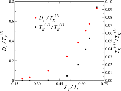
Figure 1: Characteristic energy scales. Ratio of the lower Kondo temperature $T_{K}^{(-1)}$ over the higher Kondo temperature $T_{K}^{(1)}$ (right scale, red symbols) and ratio of the critical anisotropy $D_{c}$ over higher Kondo temperature (left scale, black squares), as a function of the smaller exchange coupling $J_{-1}$ at constant larger coupling $J_{1}=0.4$.

We define the Kondo temperature $T_{K}^{(\tau)}$ as the temperature for which the contribution of channel $\tau$ to the zero-bias conductance for $D=B=0$ falls to half of its zero-temperature value [11]. For the Kondo model with channel symmetry [$J_{-1}=J_{1}$ in Eq. (1)], the topological transition takes place for $D_{c}\sim 2.5T_{K}^{(1)}$ [11], but $D_{c}$ decreases with decreasing $J_{-1}/J_{1}$ ratio. In fact, for $J_{-1}=0$ it is known to be zero [23]. In FePc experimentally $D=5$ meV [3] and $T_{K}^{(1)}\sim 20$ meV [4]. In Fig. 1 we represent the ratios $D_{c}/T_{K}^{(1)}$ and $T_{K}^{(-1)}/T_{K}^{(1)}$ for intermediate values of $J_{-1}/J_{1}$. The higher Kondo temperature $T_{K}^{(1)}$ changes only moderately as $J_{-1}/J_{1}$ varies, from 0.024 for $J_{-1}/J_{1}=0.2$ to 0.018 for $J_{-1}/J_{1}=0.7$ as a consequence of the competition between both channels [39]. Instead, $D_{c}$ and particularly $T_{K}^{(-1)}$ have a strong dependence on $J_{-1}$ in the range considered.

For comparison with experiment we take $D/W=0.01$ (that means $W\sim$ 500 meV [53], a different choice of $W$ does not affect the results in a sensitive manner) and fix $J_{1}=0.44$ so that $T_{K}^{(1)}\sim 200$ K as in experiment. The remaining parameter was fixed at $J_{-1}=0.22$ so that the system is in the non-Landau phase ($D>D_{c}$), with the width of the dip near to the experimentally observed one (as described later). The resulting Kondo temperatures are $T_{K}^{(1)}=198$ K and $T_{K}^{(-1)}=1.77$ K, while $D_{c}=0.00950\sim 4.7$ meV $\sim 55$ K.

We choose as the corresponding parameters in the auxiliary Anderson model $J_{H}=0.1$, $U_{\tau}=0.4$, $\epsilon_{\tau}=-U_{\tau}/2$, $\Delta_{1}=0.06$, $\Delta_{-1}=0.0345$. The two models have the same low-energy behavior if the results are rescaled in terms of $T_{K}^{(1)}$ or $D_{c}$.

Differential conductance at zero temperature in the absence of magnetic field

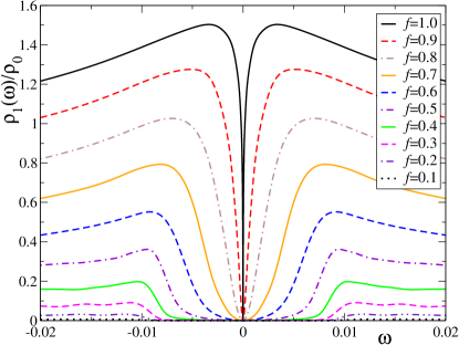
Figure 2: Variation of the spectral density as the molecule is raised from the surface. The gradual decoupling from the surface is modelled through equal reduction of both exchange coupling constants by a factor $f$. The model parameters are $J_{1}=0.44\times f$, $J_{-1}=0.22\times f$ and $D=0.01$. See Supplementary Fig. 3

for a direct comparison with experiments.

The $s$-like orbitals of the STM tip have a larger overlap with the $3z^{2}-r^{2}$ orbital of FePc than with the molecular $\pi$ orbitals and the substrate conduction-band wave functions. Ab initio calculations for Co on Cu(111) confirm this picture [64]. For this reason, the dominant contribution to the experimental $dI/dV$ spectra corresponds to the spectral density $\rho_{1}(\omega)=\rho_{1\uparrow}(\omega)+\rho_{1\downarrow}(\omega)$ in channel $\tau=1$. This description is both simpler and more physically realistic than the assumptions underlying the alternative interpretations of the measured $dI/dV$ from Refs. 4, 3, 17. The observed weak asymmetry in the line shapes indicates that some interference effects involving conduction orbitals are present. They will be incorporated in the next subsections. Here they do not modify the essential features and the conduction orbitals become less important as the molecule is raised from the surface.

Our result for FePc in the relaxed geometry corresponds to the black full line of Fig. 2 and reproduces the main features of the observed differential conductance except for some asymmetry in the experiments, which we neglect in this subsection as explained above. As the molecule is raised from the substrate by the attractive force of the STM tip, the Kondo coupling to the substrate is reduced [3]. We assume that both exchange coupling constants $J_{\tau}$ are reduced by the same factor $f$ because the same power-law dependence of the tunneling parameters $V_{\tau}$ with the distance is expected. between the localized 3d orbitals and the extended conduction states [65]. As this factor $f$ decreases from 1, the spectral density flattens and the dip broadens so that the line-shape becomes similar to that observed in single-channel Kondo systems with magnetic anisotropy [30, 31]. The exact same trend is observed experimentally [3]. For very small $f$, there should be two sharp steps at the unrenormalized threshold for inelastic spin-flip excitations ($\omega=\pm D$); in our calculations they are overbroadened due to technical reasons that limit the resolution of the NRG at large energies [66]. A detailed comparison with experiment is contained in Supplementary Note 4.

It would be interesting to push the STM tip against the molecule and tune from the tunneling to the contact regime. In this case the factor $f$ is expected to increase beyond 1 [67, 68, 69], driving the system through the topological quantum phase transition to the ordinary Fermi liquid regime. This would be signalled by the sudden transformation of the dip into a peak of similar amplitude, i.e., compared to the baseline density of states, the height of the peak just after the transition should be similar as the depth of the dip just before the transition. This is an important prediction of our theory that should be the target of future experiments (although in the contact regime, the widths of $dI/d(eV)$ and $\rho_{1}(\omega)$ may differ due to non-equilibrium effects [69]).

Temperature dependence

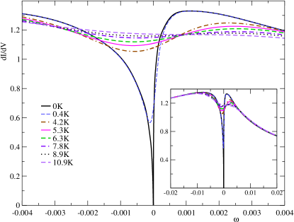
Figure 3: Temperature dependence of the differential conductance. The main panel shows the close-up on the low-energy regions, while the inset shows an extended range. Parameters as in Fig. 2. See Supplementary Fig. 4 for a direct comparison with experiments.

Assuming that the molecule is at equilibrium with the substrate, the observed differential conductance is proportional to

$$\frac{dI(V)}{dV}\propto\int d\omega\rho_{h}(\omega)f^{\prime}(\omega-eV),$$ (7)

where $f^{\prime}(\omega)$ is the derivative of the Fermi function and $\rho_{h}(\omega)$ is the density of a mixed state which contains the orbitals that have a non-vanishing hopping to the STM tip with an amplitude proportional to the hopping [70] In the present case we take only two contributions: the $3d_{3z^{2}-r^{2}}$ and the conduction states of the same symmetry. Assuming that the latter corresponds to a flat band in the absence of hybridization with the localized states, one has [71]

$$\rho_{h}(\omega)\propto\Sigma_{\sigma}\left[(1-q^{2})\text{Im}G_{1\sigma}^{d}(\omega)+2q\text{Re}G_{1\sigma}^{d}(\omega)\right],$$ (8)

where $q$ is proportional to the amplitude between the STM tip and the conduction electrons of $3z^{2}-r^{2}$ symmetry and is responsible of the observed asymmetry in the line shape. We take $q=0.4$, a similar value as taken in Refs.4, 72, although the results do not show a high sensitivity to $q.$

The temperature dependence of the dip is shown in Fig. 3. The half width of the dip at $T=0.4$ K, taken at the average between the minimum $dI/dV$ and the relative maximum near $eV=0.001$ is 3.1 K, near the reported one [3] 2.7 K. With increasing temperature, the low-energy dip in the spectral density decreases and eventually disappears, as expected. The effect is much more pronounced at low temperatures. The same trend is observed in the experiment [17]. The inset shows the results in a scale of energies similar to that of the experiment (Fig. 2 of Ref. 17). See Supplementary Note 4.

Magnetic field dependence

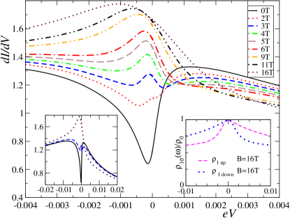
Figure 4: Magnetic field dependence of the differential conductance. Left inset: differential conductance on a wider energy scale. Right inset: spin-resolved contributions to the spectral density of the $3d_{3z^{2}-r^{2}}$ states. Parameters as in Fig. 2, with the temperature $T=0.4$ K. See Supplementary Fig. 5 for a direct comparison with experiments.

The effect of the magnetic field on the $dI/dV$ spectra reported in Ref. 17 is most striking. A moderate field of $B=11\,\mathrm{T}\sim 14\,\mathrm{K}$ readily transforms the dip into a peak with a transition near 3 to 4 T. This phenomenon is fully reproduced in our calculations, see Fig. 4. For larger fields $B>20$ T ($4.65\times 10^{-3}$) a dip s expected to form at the Fermi level as a consequence of the Zeeman splitting between $\rho_{1\uparrow}(\omega)$ and $\rho_{1\downarrow}(\omega)$. For the comparison with experimment we have taken the giromagnetic factor $g=2$, inside the range of uncertainty of previously reported values (see supplemental material of Refs. [3, 17]). A detailed comparison with experiment is contained in Supplementary Note 4.

The interpretation of this spectral transformation is highly non trivial. A field-induced topological transition from a NLFL to an OFL would result in an abrupt change from a dip into a peak, clearly at odds with the continuous evolution shown in Fig. 4 and observed in the experiment. To shed more light on this discrepancy, we investigated the Luttinger integrals entering Eqs. (4). This study was performed in terms of the equivalent auxiliary Anderson model (see Methods) and interpreted using Eqs. (5).

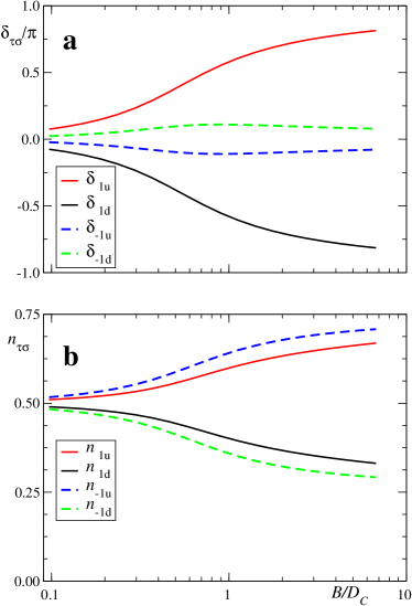
Figure 5: Evolution of impurity scattering and occupancy parameters. a Phase shifts $\delta_{\tau\sigma}$ and b occupancies $n_{\tau\sigma}$ in the auxiliary Anderson model as a function of magnetic field $B$ for $D/D_{c}=1.67$. $D_{c}$ is the anisotropy at the transition point.

In Fig. 5 a we show the evolution of the phase shifts $\delta_{\tau\sigma}$ with increasing field for $D/D_{c}>1$ (as in Figs. 2,3, and 4). For $B=0$, the four phase shifts $\delta_{\tau\sigma}=0$ (mod. $\pi$) and, therefore, the corresponding four Fermi-level spectral densities $\rho_{\tau\sigma}(0)=0$ [see Eqs. (3)]. As $B$ increases, the phase shifts for the $\pi$ molecular orbital ($\tau=-1$) change only moderately (below $0.12\pi$) and therefore, the corresponding spectral densities continue to exhibit a dip at the Fermi level. By contrast, the phase shifts that correspond to the $3z^{2}-r^{2}$ molecular orbital ($\tau=1$) change considerably, reaching the values $\pm\pi/2$ for $B/D_{c}\sim 0.8$. At this point the spectral densities $\rho_{1\sigma}(0)$ reach their maximum value. Since $\rho_{1\sigma}$ are the main contribution to the differential conductance, the above mechanism explains the transformation from a dip into a peak displayed in Fig. 4. Further increase of $B$ would lead to a Zeeman splitting, as expected for $B\gtrsim T_{K}^{(1)}$: the peak in $\rho_{1\uparrow}(\omega)$ displaces to lower energies and that in $\rho_{1\downarrow}(\omega)$ to higher energies, so that $\rho_{1\sigma}(0)$ decrease for both $\sigma$, which corresponds to $|\delta_{1\sigma}|$ increasing beyond $\pi/2$ in agreement with Eq. (3).

The changes in the spectral densities at the Fermi level with magnetic field should lead to important spatial variations of the differential conductance at small bias. For $B=0$ in the Kondo limit (integer total occupancy), the spectral densities of the localized orbitals with $\pi$ and $3z^{2}-r^{2}$ symmetry vanish at the Fermi surface and the space variation is dominated by conduction states. As $B$ increases, the influence of $\pi$ orbitals remains small but that of the cylindrical symmetric $3z^{2}-r^{2}$ orbitals increase considerably and therefore, an evolution to a more circular shape is expected, as observed experimentally [17].

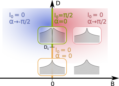
Figure 6: Schematic phase diagram of the topological properties. Phase diagram of the auxiliary Anderson model as a function of the magnetic field $B$ and the magnetic anisotropy $D$. Along the green half line $B=0$, $D>D_{c}$, the system is a non-Landau Fermi liquid (NLFL) with the topological value $I_{0}=\pi/2$, and the non-topological parameter $\alpha=0$. For an infinitesimal $B$ both quantities jump as indicated in the figure, yet all physical quantities are continuous. For $D<D_{c}$, $I_{0}=0$, and $\alpha$ is continuous across $B=0$, where its value crosses zero (orange segment). The insets show the low-energy region around the Fermi level: regular Fermi liquid (orange frame) and NLFL (green frame) at zero magnetic field, as well as weakly spin-polarized Fermi liquids at moderate magnetic field (white and pink frame).

The topological properties under an applied magnetic field are very peculiar. For $B=0$ and $D>D_{c}$, there is a pole in the self-energy $\Sigma(\omega)$ on the real axis at $\omega=0$. An infinitesimal $B$ displaces this pole away from $\omega=0$, as it is shown in Supplementary Note 3. $I_{0}$ drops to zero and the system becomes an OFL. However at the same time $\alpha$ jumps to $\pi/2$ ($-\pi/2$) for infinitesimal positive (negative) $B$. See Fig. 6. As a result, in both cases the Luttinger integral $I_{-1\sigma}$ for the majority spin [that is $\uparrow$ ($\downarrow$) for positive (negative) $B$] remains $\pi/2$, while $I_{1\sigma}$ jumps from $\pi/2$ to $-\pi/2$, see Eqs. (6). This jump in $\pi$ does not affect any physical properties which are continuous across $B=0$, as expected and in-line with the “modulo $\pi$ ambiguity” in the definition of the scattering phase shifts [59]. The Luttinger integrals for minority spin are obtained by interchanging the orbital index.

For $D<D_{c}$, $I_{0}$ and $\alpha$ are continuous as functions of $B$, and both are equal to zero for $B=0$. In fact, in the whole $(D,B)$ plane, $I_{0}\equiv 0$ and $\alpha$ is continuous except on the half-line $B=0$, $D>D_{c}$. This line is, hence, a branch-cut for $\alpha$. See Fig. 6. Furthermore, the point $D=D_{c}$, $B=0$ may be considered as a logarithmic singularity for the function $\alpha(D,B)$ viewed as a function in the complex plane with the argument $z=D+iB$. In Fig. 7 we display $\alpha$ as a function of both $D/D_{c}$ and $B/D_{c}$. As explained above for $B\rightarrow 0^{+}$, $\alpha(D,B=0)=(\pi/2)\theta(D-D_{c})$, where $\theta(x)$ is the step function. For small non-zero $B$, $\alpha(D,B)$ still resembles this step function. In fact, $\alpha(D,B)\sim-\frac{1}{2}\mathrm{Im}\ln[D_{c}-D-iB]$. As $|B|$ further increases, $\alpha(D)$ decreases markedly for $D>D_{c}$. For $|B|\gg D_{c}$, $\alpha$ is small for all $D$ and as a consequence also the four Luttinger integrals are small.

As $|B|$ increases, the occupancies $\left\langle n_{\tau\uparrow}\right\rangle$ increase [see Fig. 5 b], with the effect of increasing $\delta_{\tau\uparrow}$ [see Eqs. (4)]. For $\delta_{-1\uparrow}$, this effect is largely compensated by the decrease in $\alpha$, leading to a small overall variation of the phase shift. Instead, for $\delta_{1\uparrow}$ both effects add up and $\delta_{1\uparrow}$ has a marked increase, which is then reflected in the transformation of the dip into a peak. For spin $\downarrow$ the effects are opposite.

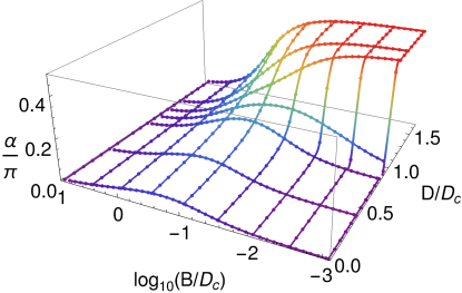
Figure 7: Non-topological parameter. Phase shift $\alpha(D,B)$ for the auxiliary Anderson model as a function of magnetic anisotropy $D$ and magnetic field $B$. The color encodes the value of $\alpha$.

Discussion

The ability to flip the differential conductance between low and high values by tuning some external parameter is of tremendous practical importance in molecular electronics for switching device applications. Recently a topological quantum phase transition has been found in a spin-1 Kondo model with two degenerate channels and single-ion magnetic anisotropy, in which the zero-bias differential conductance and the spectral density at zero temperature jump from their maximum possible values to zero as the longitudinal single-ion anisotropy $D$ is increased beyond a threshold value $D_{c}$ [11, 12]. By generalizing the theory of such topological transitions to nonequivalent channels and finite magnetic field, we have for the first time conclusively identified FePc/Au(111) as an experimental realization of this phenomenon, since our approach provides a unified description of the totality of experimental observations. The main difficulty in this identification is that for $D>D_{c}$ the system is an unconventional Fermi liquid that cannot be adiabatically connected to a non-interacting system by turning off the interactions [11, 12, 13, 14]. The corresponding concept of a non-Landau Fermi liquid (NLFL) remains largely unfamiliar to most of the physics community. In the NLFL, the Friedel sum rule has to be generalized by introducing a topological quantity that has been previously overseen, even though it leads to a dramatic drop in spectral density and differential conductance for $D>D_{c}$.

By formulating a general theory of the topological aspects of the Friedel sum rule that incorporates the effects of broken channel and spin symmetries, fully corroborated by numerical calculations for a model Hamiltonian, we reliably established that FePc on Au(111) behaves as a NLFL. With a single set of parameters we explained three key experiments on the differential conductance of this system [4, 3, 17]. The sole assumption (i.e., that the scanning tunneling microscope senses mainly the 3d orbital of Fe with $3d^{2}-r^{2}$ symmetry) is simple, physically realistic, and consistent with ab initio calculations [64]

The same model also explains the recent experiments for MnPc on Au(111) [38], which exhibit a dependence on magnetic field with qualitative features similar to those in FePc on Au(111). Alternative explanations proposed for these experiments are questionable or contradict well established facts, like the role of Hund rules in defining ground-state multiplets.

While a moderate magnetic field $B$ of the order of 10 T leads to a continuous transition from very small to very high zero-bias conductance, we predict an abrupt transition for $B=0$ if the tip is pressed against the molecule changing the regime of the system from the tunneling to the contact one, thereby increasing the Kondo temperatures [67, 68, 69].

Methods

The numerical calculations were performed with the NRG Ljubljana [73, 74] implementation of the numerical renormalization group method [66, 75] using the separate conservation of the isospin (axial charge) in each channel $\tau$, as well as the conservation of the $z$-component of the total spin, i.e., $SU(2)\times SU(2)\times U(1)$ symmetry. The calculations for the Kondo model were performed with the discretization parameter $\Lambda=4$ with the broadening parameter $\alpha=0.8$ for Figs. 3 and 4. For Fig. 2 the values of $\alpha$ used were 0.1 for $f\leq 0.1$, 0.2 for $f=0.6$ and 0.7, 0.4 for $f=0.8$ and 0.9 and 0.6 for $f=1$. The calculations for the Anderson model have been performed using $\Lambda=3$ with the broadening parameter $\alpha=0.3$. We kept up to 10000 multiplets (or up to cutoff 10 in energy units) in the truncation, averaging over $N_{z}=4$ different discretization meshes. The spectral functions were computed using the complete Fock space algorithm [76], and the resolution for the Anderson model was improved using the “self-energy trick” [77].

For large interaction $U$, the value of $D_{c}$ calculated with the Anderson model Eq. (2) coincides with that obtained from the corresponding Kondo model, However, for example for $U=4$, we obtain that the phase shift modulo $\pi$ calculated directly from the NRG spectrum and that obtained the using the generalized Friedel sum rule Eqs. (4) deviate by up to $0.1\pi$ for large $B$. This is due to the fact that Eqs. (4) were simplified for the case in which the conduction band width (which we have taken as $2W=2$) is much larger than all other energies involved (the “wide-band limit”), in such a way that the number of conduction electrons per channel is not modified by the addition of the impurity [9]. To avoid this difficulty, we have used $U=0.4$ in the calculations with the Anderson model. In this case the maximum deviation between both phase shifts is below $0.02\pi$ and the critical anisotropy is reduced by a factor of the order of 6. However, the physical properties are very similar for the same $D/D_{c}$ and $B/D_{c}$.

Data availability

The datasets generated during the current study are available in the Zenodo repository under accession code 10.5281/zenodo.5506654. The data includes figure sources and model definition files for the NRG solver.

Code availability

The NRG calculations presented in this work have been performed with the NRG Ljubljana code. The source code is available from GitHub, https://github.com/rokzitko/nrgljubljana. A snapshot of the specific version used (8f90ac4) has been posted on Zenodo, http://doi.org/10.5281/zenodo.4841076.

Author contributions

A. A. A. and L. O. M. conceived the project, R. Ž. and G. G. B. performed the NRG calculations. A. A. A., R. Ž. and L. O. M. wrote the paper.

Competing Interests

The authors declare no competing interests.

Supplementary Note 1: Auxiliary multiorbital two-channel Anderson model

In order to analyze the topological features of the $S=1$ Kondo model (1) with two non-equivalent channels, encoded in the generalized Friedel sum rules that we will deduce in Supplementary Note 2, it is better to work with the auxiliary multiorbital two-channel Anderson Hamiltonian,

$$H_{A}=H_{0}+H_{\rm int}.$$ (9)

$H_{0}$ contains the one-body terms:

$$H_{0}=H_{\rm cond}+H_{\rm hyb}+H_{d}.$$ (10)

$H_{\rm cond}$ corresponds to two conduction bands (channels): one with symmetry $3z^{2}-r^{2}$ ($\tau=1$) and another that takes into account the degenerate $\pi$-manifold $xz,yz$ ($\tau=-1$) [3]:

$$H_{\rm cond}=\sum_{k\tau\sigma}\varepsilon_{k\tau}{c}^{\dagger}_{k\tau\sigma}{c}_{k\tau\sigma};$$ (11)

we consider conduction electron energy dispersions such that both bands have the same constant density of states (DOS) and we work in the wide-band limit, such that the half-bandwidth $W$ is the largest energy scale in the problem.

$H_{\rm hyb}$ contains the hybridization between the conduction and impurity states with the same $\tau$ symmetry:

$$H_{\rm hyb}=\sum_{k\tau}\left(V_{\tau}{c}^{\dagger}_{k\tau\sigma}{d}_{\tau\sigma}+{\rm H.c.}\right).$$ (12)

For correct description of FePc on Au(111), it is essential to allow for very different coupling strenghts $V_{\tau}$ of each localized orbital with the substrate, giving rise to a multiorbital Anderson model with non-equivalent orbitals. Due to its spatial dependence, the $\tau=1$ localized orbital hybridizes stronger with the gold surface than the $\tau=-1$ orbital. As a consequence, $V_{1}>V_{-1}$.

$H_{d}$ includes the impurity single-orbital (hole) energies and the Zeeman term:

$$H_{d}=\sum_{\tau\sigma}\epsilon_{\tau}n_{\tau\sigma}-BS_{z}\equiv\sum_{\tau\sigma}\epsilon_{\tau\sigma}n_{\tau\sigma},\;\;{\rm with}\;\;\epsilon_{\tau\sigma}\equiv\epsilon_{\tau}-\sigma\frac{B}{2}.$$ (13)

We consider a Zeeman term only at the impurity site because for constant conduction-band DOS in the wide-band limit, the magnetic field has no effect on the conduction band (i.e., it can be eliminated through a simple energy shift).

The interaction terms act on the impurity states:

$$H_{\rm int}=\sum_{\tau}U_{\tau}n_{\tau\uparrow}n_{\tau\downarrow}-J_{H}{\bm{S}}_{1}\cdot{\bm{S}}_{-1}+D\left(\sum_{\tau}{S}_{z\tau}\right)^{2}.$$ (14)

We study this model in the particle-hole symmetric case, corresponding to $\epsilon_{\tau}=-\frac{U_{\tau}}{2}$ and symmetric conduction bands relative to the $\omega=0$ Fermi level) in order to have exactly one hole in each impurity orbital. In the Kondo regime, $-\epsilon_{\tau}\gg V^{2}_{\tau}/W$, these two holes are ferromagnetically coupled by the first Hund’s rule, $J_{H}>0$, yielding an effective $S=1$ at the impurity site. Due to symmetry considerations of the involved 3d orbitals, we take the same Hubbard repulsion $U$ for each impurity orbital. This implies that both single-orbital energies $\epsilon_{\tau}$ should be degenerate in the particle-hole symmetric case, while ab initio calculations [4] give an energy difference of the order of 1 eV. In the Kondo regime this difference is irrelevant.

Among the interactions of a generic multiorbital Anderson Hamiltonian for 3d impurities [5], we are neglecting the inter-orbital Hubbard repulsion $U^{\prime}n_{1}n_{-1}$, as this term is almost constant in the (particle-hole symmetric) Kondo regime. We also neglect the pair hopping interaction $J_{H}({d}^{\dagger}_{1\uparrow}{d}^{\dagger}_{1\downarrow}{d}_{-1\downarrow}{d}_{-1\uparrow}+{\rm H.c.})$, as, for FePc on Au(111), the two-electron low energy sector contains only the triplet states due to the strong Hund’s coupling [4]. While the inter-orbital Hubbard repulsion $U^{\prime}$ could be easily included in the NRG computation, the pair hopping interaction breaks the separate conservation of the isospin in each channel $\tau$, resulting in a very demanding computational effort.

By means of the equation of motion method, it can be shown [6] that all the conduction band information needed for the computation of impurity observables is encoded in the hybridization functions

$$\Delta_{\tau}(\omega)=\pi\sum_{k}V_{\tau}^{2}\delta(\omega-\varepsilon_{k\tau}).$$ (15)

As we assume equal constant conduction-band DOS for boths channels and energy-independent $V_{\tau}$, the hybridisation functions $\Delta_{\tau}$ are likewise constant functions. This is a very reliable assumption for normal conduction bands with a finite DOS at the Fermi level, as in this case the Kondo physics depend only marginally on the exact form of the DOS. It should be stressed that, if we were interested in substrate observables like STM spectra far from the impurity, there would be a need for a more thorough modeling of the conduction bands and the tunneling parameters $V_{\tau}$.

It is worth to mention that, in the Kondo regime, the Anderson Hamiltonian (9) can be exactly mapped to the Kondo Hamiltonian (1) by means of the Schrieffer-Wolff transformation [6], with Kondo exchange interactions given by $J_{\tau}=4V_{\tau}^{2}/U$. Potential scattering is absent due to the particle-hole symmetry. We have numerically verified the agreement between the predictions for both Hamiltonians. Although the Kondo model is simpler because of its reduced local Hilbert space, it is better to work with the auxiliar Hamiltonian (9) in order to clearly interpret the Friedel sum rules, which involves the computation of the localized spin-orbital occupancies $\langle n_{\tau\sigma}\rangle$.

Conservation laws for the Anderson Hamiltonian

The Hamiltonian $H_{A}$ commutes with the total electron number per orbital

$$N_{\tau}=\sum_{k\sigma}{n}_{k\tau\sigma}+\sum_{\sigma}{n}_{\tau\sigma}$$ (16)

($n_{k\tau\sigma}\equiv c^{\dagger}_{k\tau\sigma}c_{k\tau\sigma}$) and with the total electron number per spin

$${N}_{\sigma}=\sum_{k\tau}{n}_{k\tau\sigma}+\sum_{\tau}{n}_{\tau\sigma}.$$ (17)

Consequently, the system conserves the total electron number,

$$N=\sum_{\tau\sigma}{N}_{\tau\sigma},$$ (18)

the total spin projection along the $z$ direction,

$${S}^{\rm tot}_{z}=\frac{1}{2}\sum_{\tau\sigma}\sigma{N}_{\tau\sigma},$$ (19)

and the total orbital isospin

$${T}_{z}=\sum_{\tau\sigma}\tau N_{\tau\sigma}.$$ (20)

As there are no spin-orbit couplings and the magnetic field $B$ is along the single-ion anisotropy axis $z$, the Hamiltonian $H_{A}$ also commutes with the total spin

$${\bm{S}}^{2}=\frac{1}{2}\left({S}_{+}{S}_{-}+{S}_{-}{S}_{+}\right)+\left({S}_{z}\right)^{2},$$ (21)

where $S_{+}=\sum_{\tau}\left(\sum_{k}c^{\dagger}_{k\tau\uparrow}c_{k\tau\downarrow}+d^{\dagger}_{\tau\uparrow}d_{\tau\downarrow}\right),$ $S_{-}=(S_{+})^{\dagger}$. It is worth to mention that if the single-particle energies $\varepsilon_{k\tau\sigma}$ and $\epsilon_{\tau\sigma}$ in $H_{0}$ were arbitrary, the total spin ${\bm{S}}^{2}$ would commute with $H_{A}$ only if the relations $\varepsilon_{\mu\tau\uparrow}-\varepsilon_{\mu\tau\downarrow}=\varepsilon_{\mu^{\prime}\tau^{\prime}\uparrow}-\varepsilon_{\mu^{\prime}\tau^{\prime}\downarrow}$ hold for all $\mu,\mu^{\prime}=k,d;\tau,\tau^{\prime}=1,-1$.

Supplementary Note 2: Generalized Friedel sum rules

Green’s functions and electron occupation numbers

Under the conservation laws (19), (20), it can be shown by means of the Lehmann representation that all the single-particle Green’s functions (GF) of $H_{A}$ ,

$$G^{kk^{\prime}}_{\tau\sigma\tau^{\prime}\sigma^{\prime}}\equiv<\!\!\!<c_{k\tau\sigma}|c^{\dagger}_{k^{\prime}\tau^{\prime}\sigma^{\prime}}>\!\!\!>,\;\;G^{kd}_{\tau\sigma\tau^{\prime}\sigma^{\prime}}\equiv<\!\!\!<c_{k\tau\sigma}|d^{\dagger}_{\tau^{\prime}\sigma^{\prime}}>\!\!\!>,\;\;$$

$$G^{dk^{\prime}}_{\tau\sigma\tau^{\prime}\sigma^{\prime}}\equiv<\!\!\!<d_{\tau\sigma}|c^{\dagger}_{k^{\prime}\tau^{\prime}\sigma^{\prime}}>\!\!\!>,\;\;G^{d}_{\tau\sigma\tau^{\prime}\sigma^{\prime}}\equiv<\!\!\!<d_{\tau\sigma}|d^{\dagger}_{\tau^{\prime}\sigma^{\prime}}>\!\!\!>,$$

are diagonal in spin and orbital indices. Thus, the GF matrix is block diagonal:

$$\bm{\mathbb{G}}=\left(\begin{array}[]{cccc}\bm{\mathbb{G}}_{1\uparrow}&0&0&0\\ 0&\bm{\mathbb{G}}_{1\downarrow}&0&0\\ 0&0&\bm{\mathbb{G}}_{-1\uparrow}&0\\ 0&0&0&\bm{\mathbb{G}}_{-1\downarrow}\end{array}\right),$$ (22)

where the block indices run over the conduction electron momenta and the impurity, that is, over the set $I\equiv\left\{k_{1},k_{2},\cdots,d\right\}$.

As the interaction terms involve only the impurity degrees of freedom, we can express the conduction-band and mixed Green’s functions in terms of the impurity GF $G^{d}$ using the equations of motion. We have

$$G^{kk^{\prime}}_{\tau\sigma} = g_{k\tau}+|V_{\tau}|^{2}g_{k\tau}G^{d}_{\tau\sigma}g_{k^{\prime}\tau},$$

$$G^{kd}_{\tau\sigma} = V_{\tau}g_{k\tau}G^{d}_{\tau\sigma},$$ (23)

$$G^{dk^{\prime}}_{\tau\sigma} = V^{*}_{\tau}g_{k^{\prime}\tau}G^{d}_{\tau\sigma},$$

where

$$g_{k\tau}=\frac{1}{z-\varepsilon_{k\tau}}.$$ (24)

The total electron numbers per spin and per orbital can be expressed as the complex-plane contour integrals [7]

$$\langle{N}_{\tau\sigma}\rangle=\oint_{\Gamma}\frac{dz}{2\pi i}n_{F}(z){\rm Tr}\;{\bm{\mathbb{G}}}_{\tau\sigma}(z),$$ (25)

where $n_{F}$ is the Fermi function and the contour $\Gamma$, shown in Supplementary Fig. S1, encloses all the poles of the GF matrix (along the real axis) and none of the poles of $n_{F}$ (along the imaginary axis).

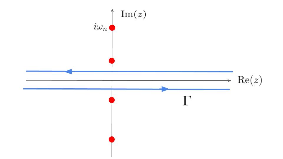
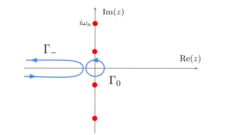
Figure S1: Integration contours in the complex plane. a) $\Gamma$ encloses all the real axis; b) $\Gamma_{0}$, the origin of the complex plane, and $\Gamma_{-}$, the negative real axis. The dots represent the fermionic Matsubara frequencies $i\omega_{n}=i\frac{(2n+1)\pi}{\beta}$.

Using (22) and (23), we get

$${\rm Tr}\;{\bm{\mathbb{G}}}_{\tau\sigma}(z)=\sum_{k}G^{kk}_{\tau\sigma}(z)+G^{d}_{\tau\sigma}(z)=\sum_{k}g_{k\tau}+\sum_{k}\frac{\left|V_{\tau}\right|^{2}}{(z-\varepsilon_{k\tau})^{2}}G^{d}_{\tau\sigma}(z)+G^{d}_{\tau\sigma}(z).$$ (26)

If we define the complex hybridization function

$$\Gamma_{\tau}(z)\equiv\sum_{k}\frac{\left|V_{\tau}\right|^{2}}{z-\varepsilon_{k\tau}},$$ (27)

then

$${\rm Tr}\;{\bm{\mathbb{G}}}_{\tau\sigma}(z)=\sum_{k}\frac{1}{z-\varepsilon_{k\tau}}+\left(1-\frac{\partial\Gamma_{\tau}(z)}{\partial z}\right)G^{d}_{\tau\sigma}(z).$$ (28)

Now we re-express the trace of the GF matrix in terms only of impurity functions (GF and self-energy). Using the formula 

$$\det{\mathbb{G}}_{\tau\sigma}=\left(\prod_{k}g_{k\tau}\right)G^{d}_{\tau\sigma},$$ (29)

and the impurity Dyson equation

$$(G^{d}_{\tau\sigma})^{-1}=z-\epsilon_{\tau\sigma}-\Gamma_{\tau}(z)-\Sigma^{d}_{\tau\sigma}(z),$$ (30)

where $\Sigma^{d}_{\tau\sigma}$ is the impurity self-energy due to the interaction terms (14), we obtain

$$\frac{\partial\ln\det{\bm{\mathbb{G}}}^{-1}_{\tau\sigma}}{\partial z}=\sum_{k}\frac{\partial\ln g^{-1}_{k\tau}}{\partial z}+\frac{\partial\ln(G^{d}_{\tau\sigma})^{-1}}{\partial z}=\sum_{k}g_{k\tau}+\left(1-\frac{\partial\Gamma_{\tau}}{\partial z}-\frac{\partial\Sigma^{d}_{\tau\sigma}}{\partial z}\right)G^{d}_{\tau\sigma}.$$ (31)

Therefore,

$${\rm Tr}\;{\mathbb{G}}_{\tau\sigma}=\frac{\partial\ln\det{\mathbb{G}}^{-1}_{\tau\sigma}}{\partial z}+G^{d}_{\tau\sigma}(z)\frac{\partial\Sigma^{d}_{\tau\sigma}(z)}{\partial z},$$ (32)

and the electron numbers are given by

$$\langle{N}_{\tau\sigma}\rangle=\oint_{\Gamma}\frac{dz}{2\pi i}n_{F}(z)\frac{\partial\ln\det{\mathbb{G}}^{-1}_{\tau\sigma}}{\partial z}+\oint_{\Gamma}\frac{dz}{2\pi i}n_{F}(z)G^{d}_{\tau\sigma}(z)\frac{\partial\Sigma^{d}_{\tau\sigma}(z)}{\partial z}.$$ (33)

Generalized Friedel sum rules and Luttinger integrals

Here, we generalize the Friedel sum rules for multiorbital models using the conservation laws studied by Yoshimori and Zawadowski [8]. The first integral in the Supplementary Eq. (33) for the electron numbers can be rewritten, using (31), as

$$\sum_{k}\oint_{\Gamma}\frac{dz}{2\pi i}n_{F}(z)g_{k\tau}(z)+\oint_{\Gamma}\frac{dz}{2\pi i}n_{F}(z)\frac{\partial\ln(G^{d}_{\tau\sigma})^{-1}}{\partial z}\equiv\langle N_{\rm\tau\sigma}^{{\rm c}(0)}\rangle+\oint_{\Gamma}\frac{dz}{2\pi i}n_{F}(z)\frac{\partial\ln(G^{d}_{\tau\sigma})^{-1}}{\partial z},$$ (34)

where $\langle N_{\rm\tau\sigma}^{{\rm c}(0)}\rangle$ are the conduction electron numbers in the absence of the impurity. In the wide-band limit, the number of conduction electrons remains unaltered when the impurity is introduced. As a consequence $\langle N_{\rm\tau\sigma}\rangle-\langle N_{\rm\tau\sigma}^{{\rm c}(0)}\rangle=\langle n_{\tau\sigma}\rangle$. On the other hand, the last integral in (34), in the zero temperature limit, is

$$\lim_{T\to 0}\oint_{\Gamma}\frac{dz}{2\pi i}n_{F}(z)\frac{\partial\ln(G^{d}_{\tau\sigma})^{-1}}{\partial z}=-\frac{1}{\pi}{\rm Im}\;\int_{-\infty}^{0}\frac{\partial\ln(G^{d}_{\tau\sigma})^{-1}}{\partial\omega}d\omega=\frac{1}{\pi}{\rm Im}\ln G^{d}_{\tau\sigma}(0)-\frac{1}{\pi}{\rm Im}\ln G^{d}_{\tau\sigma}(-\infty)=\frac{\delta_{\tau\sigma}}{\pi},$$ (35)

where we have defined the (Fermi level) phase shift $\delta_{\tau\sigma}$ [9] through

$$G^{d}_{\tau\sigma}(0)=-|G^{d}_{\tau\sigma}(0)|e^{i\delta_{\tau\sigma}}.$$

Putting all these ingredients together we obtain the generalized Friedel sum rules, that relate the quasiparticle phase shifts and the impurity occupancies at zero $T$,

$$\delta_{\tau\sigma}=\pi\langle n_{\tau\sigma}\rangle+I_{\tau\sigma},$$ (36)

with the Luttinger integrals $I_{\tau\sigma}$ [10] defined as

$$I_{\tau\sigma}={\rm Im}\int_{-\infty}^{0}G^{d}_{\tau\sigma}\frac{\partial\Sigma^{d}_{\tau\sigma}}{\partial\omega}d\omega.$$ (37)

Until very recently, it had been considered that the vanishing of the Luttinger integrals represents one of the hallmarks of Fermi liquid phases [10, 9]. In this way, the (ordinary) Friedel sum rules state that the quasiparticle phase shifts are simply the impurity occupancies divided by $\pi,$ as it was known from the fifties. However, in the last two years, it was shown that, for certain single-impurity [11, 12] and two-impurity [13, 14] models, the Luttinger integrals can take the discrete values $\pm\pi/2$ in the so-called non-Landau Fermi liquids (NLFL), that is, Fermi liquid phases that are not adiabatically connected with their non-interacting counterparts [11]. In this work we have found that an iron phthalocyanine molecule on Au(111) behaves as a NLFL in the absence of an applied magnetic field, while for $B\neq 0$ it is an “ordinary” Fermi liquid, but with non-zero Luttinger integrals that change continuosly with $B$. So, we have shown that there are Fermi liquids in which the Friedel sum rules (36) holds only in its generalized version with non-zero (continuous) Luttinger integrals.

As the impurity spectral function at the Fermi level is

$$\rho_{\tau\sigma}(0)=-\frac{1}{\pi}{\rm Im}G^{d}_{\tau\sigma}(0)=\frac{1}{\pi}|G^{d}_{\tau\sigma}(0)|\sin(\delta_{\tau\sigma}),$$ (38)

for a Fermi liquid whose low (but finite) energy behavior is characterized by ${\rm Im}\Sigma^{d}_{\tau\sigma}\propto-a\omega^{2}$ ($a>0$). This results in $|G^{d}_{\tau\sigma}(\omega\to 0)|=\sin\delta_{\tau\sigma}/\Delta_{\tau}$. Consequently, the Friedel sum rule for spectral functions, valid for Fermi liquids, is given by

$$\rho_{\tau\sigma}(0)=\frac{1}{\pi\Delta_{\tau}}\sin^{2}\delta_{\tau\sigma}.$$ (39)

The above argument remains valid if the imaginary part of the self-energy has a Dirac $\delta$ centered exactly at the Fermi level, as it happens in the NLFL [11] where ${\rm Im}\Sigma^{d}_{\tau\sigma}=-a\omega^{2}-b\delta(\omega)$. The generalized Friedel sum rule for the spectral funcion $\rho_{\tau\sigma}(\omega\to 0)$ (39) therefore holds even for the NLFL.

Topological interpretation of the Luttinger integrals

Here, we demonstrate that for certain Anderson impurity models (single-orbital, degenerate two-orbital with an arbitrary magnetic field, non-equivalent two-orbital model without magnetic field), the Luttinger integrals have a topological nature. For this purpose, we turn off the interactions of the Anderson Hamiltonian $H_{A}$. The total electron numbers can change as the interactions are turned off. Using (33) the electron numbers in the non-interacting case are

$$\langle{N}_{\tau\sigma}\rangle^{0}=\oint_{\Gamma}\frac{dz}{2\pi i}n_{F}(z)\frac{\partial\ln\det({\mathbb{G}^{(0)}}_{\tau\sigma})^{-1}}{\partial z},$$ (40)

where ${\mathbb{G}^{(0)}}_{\tau\sigma}$ are the non-interacting GF block matrices. One should not confound these electron numbers, corresponding to the non-interacting Anderson model ($H=H_{0}$, i.e. setting $H_{\mathrm{int}}=0$) with the impurity still hybridized with the conduction channels, with the previously defined $\langle N_{\tau\sigma}^{{\rm c}(0)}\rangle$ (Supplementary Eq. 34) that correspond to the conduction electron numbers for the case of decoupled impurity (i.e., setting $H_{\rm hyb}=0$).

From (33) and (40), we obtain

$$\langle{N}_{\tau\sigma}\rangle-\langle{N}_{\tau\sigma}\rangle^{0}=\oint_{\Gamma}\frac{dz}{2\pi i}n_{F}(z)\frac{\partial\ln D_{\tau\sigma}}{\partial z}+\oint_{\Gamma}\frac{dz}{2\pi i}n_{F}(z)G^{d}_{\tau\sigma}(z)\frac{\partial\Sigma^{d}_{\tau\sigma}(z)}{\partial z},$$ (41)

where we have defined the scalar function

$$D_{\tau\sigma}(z)=\frac{\det{\mathbb{G}^{(0)}}_{\tau\sigma}}{\det{\mathbb{G}}_{\tau\sigma}}.$$ (42)

Taking into account (29), its expression is simplied to

$$D_{\tau\sigma}(z)=\frac{G^{d(0)}_{\tau\sigma}(z)}{G^{d}_{\tau\sigma}(z)}.$$ (43)

For $T\to 0$, it can be shown [15] that the integral

$$n_{D}({\Gamma})\equiv\oint_{\Gamma}\frac{dz}{2\pi i}n_{F}(z)\frac{\partial\ln D_{\tau\sigma}}{\partial z}$$ (44)

is a winding number. When $T\to 0$, the vanishing of the Fermi function for ${\rm Re}\;z>0$ turns ${\Gamma}$ into the curve ${\Gamma}_{-}\cup{\Gamma}_{0}$ that encircle only the negative real axis and the origin (see Supplementary Fig. S1), and

$$n_{D}({\Gamma}) \to n_{D}(\Gamma_{-})+\frac{1}{2}n_{D}(\Gamma_{0})=$$

$$= \oint_{\Gamma_{-}}\frac{dz}{2\pi i}\frac{\partial\ln D_{\tau\sigma}(z)}{\partial z}+\frac{1}{2}\oint_{{\Gamma_{0}}}\frac{dz}{2\pi i}\frac{\partial\ln D_{\tau\sigma}(z)}{\partial z}=$$

$$= \frac{1}{2\pi i}\oint_{{\cal D}_{\Gamma_{-}}}\frac{dD_{\tau\sigma}}{D_{\tau\sigma}}+\frac{1}{2}\times\frac{1}{2\pi i}\oint_{{\cal D}_{\Gamma_{0}}}\frac{dD_{\tau\sigma}}{D_{\tau\sigma}},$$

where ${\cal D}_{\Gamma_{-}}$ (${\cal D}_{\Gamma_{0}}$) is the closed curve that describes $D(z),$ as $z$ goes along ${\Gamma}_{-}$ ($\Gamma_{0}$) in the complex plane $({\rm Re}\;D,{\rm Im}\;D)$. $n_{D}({\Gamma_{-}}),n_{D}(\Gamma_{0})$ are the winding numbers of $D$ around the origin for paths $\Gamma_{-}$ and $\Gamma_{0}$, respectively. These numbers are integer (positive if $D$ winds counterclockwise around the origin, negative in the other direction). The $1/2$ factor that multiply $n_{D}(\Gamma_{0})$ comes from $n_{F}(z=0)=\frac{1}{2}$.

In the $T\to 0$ limit we can use the relations [7]

$$\lim_{T\to 0}\oint_{\Gamma}\frac{dz}{2\pi i}n_{F}(z)F(z)=-\frac{1}{\pi}{\rm Im}\;\int_{-\infty}^{0}F(\omega)d\omega$$ (46)

to get, from (41),

$$\langle{N}_{\tau\sigma}\rangle-\langle{N}_{\tau\sigma}\rangle^{0}=-\frac{1}{\pi}{\rm Im}\;\int_{-\infty}^{0}\frac{\partial\ln D_{\tau\sigma}}{\partial\omega}d\omega-\frac{1}{\pi}I_{\tau\sigma}.$$ (47)

The integral can be expressed in terms of winding numbers (Topological interpretation of the Luttinger integrals), that is,

$$\langle{N}_{\tau\sigma}\rangle-\langle{N}_{\tau\sigma}\rangle^{0}=n_{D}(\Gamma_{-})+\frac{1}{2}n_{D}(\Gamma_{0})-\frac{1}{\pi}I_{\tau\sigma}.$$ (48)

From this we deduce that if the total electron numbers do not change when the interactions are turned off, the Luttinger integrals only take discrete values that are multiples of $\pi/2$:

$$I_{\tau\sigma}=\pi n_{D}(\Gamma_{-})+\frac{\pi}{2}n_{D}(\Gamma_{0}).$$ (49)

Note that $n_{D}(\Gamma_{0})$ is different from zero if $D(z)$ has a zero or a pole at $z=0$. For example, if $D(z)=z$ or $1/z$ and we take $\Gamma_{0}$ as a circle of radius $R$ centered in the origin, then

$$n_{D}(\Gamma_{0})=\frac{1}{2\pi i}\lim_{R\to 0}\oint_{\Gamma_{0}(R)}\frac{dD}{D}=\frac{1}{2\pi i}\int_{0}^{2\pi}\frac{(\pm i)Re^{\pm i\theta}d\theta}{Re^{\pm i\theta}}=\pm 1.$$ (50)

Effective one-body Hamiltonian

If, as it can in general be expected, $\langle{N}_{\tau\sigma}\rangle\neq\langle{N}_{\tau\sigma}\rangle^{0},$ we can try to tune the effective impurity one-body energies (chemical potential, magnetic field, crystal-field) in order to force the same interacting and non-interacting electron numbers. If this is possible, we will show that the Luttinger integrals keep their topological nature. We define an effective one-body impurity Hamiltonian $\tilde{H}_{d}$

$$\tilde{H}_{d}=\sum_{\tau\sigma}\left(\tilde{\epsilon}-\frac{\sigma}{2}\tilde{B}+\tau\tilde{C}\right)n_{\tau\sigma}\equiv\sum_{\tau\sigma}\tilde{\epsilon}_{\tau\sigma}{n}_{\tau\sigma}.$$ (51)

The dependence of the single-particle energy $\tilde{\epsilon}_{\tau\sigma}$ on $\sigma$ and $\tau$ is dictated by the requirement that the effective Hamiltonian obey the same conservation laws (see Supplementary Note 1) as the original Anderson Hamiltonian.

To go further we re-arrange the non-interacting and interacting terms of the impurity Hamiltonian:

$${H}_{\rm imp}={H}_{d}+{H}_{\rm int}=\tilde{H}_{d}+\tilde{H}_{\rm int},$$ (52)

with

$$\tilde{H}_{d}=\sum_{\tau\sigma}\tilde{\epsilon}_{\tau\sigma}{n}_{\tau\sigma}={H}_{d}+\sum_{\tau\sigma}\left(\tilde{\epsilon}_{\tau\sigma}-\epsilon_{\tau\sigma}\right){n}_{\tau\sigma},$$ (53)

while

$$\tilde{H}_{\rm int}={H}_{\rm int}+\sum_{\tau\sigma}\left(\epsilon_{\tau\sigma}-\tilde{\epsilon}_{d\tau\sigma}\right){n}_{\tau\sigma}.$$ (54)

As the Hamiltonian remains unaltered, the impurity Green function does not change. However, there is a rearrangement of its “non-interacting” and “interacting” contributions:

$$(G^{d}_{\tau\sigma})^{-1}=(G^{d(0)}_{\tau\sigma})^{-1}-\Sigma^{d}_{\tau\sigma}=z-\epsilon_{\tau\sigma}-\Gamma_{\tau}-\Sigma^{d}_{\tau\sigma}=$$ (55)

$$=z-\tilde{\epsilon}_{\tau\sigma}-\Gamma_{\tau}-\Sigma^{d}_{\tau\sigma}+(\tilde{\epsilon}_{\tau\sigma}-{\epsilon}_{\tau\sigma})=(\tilde{G}^{d(0)}_{\tau\sigma})^{-1}-\tilde{\Sigma}^{d}_{\tau\sigma},$$ (56)

where the renormalized self-energy is defined as the original one shifted by a constant real number (a Hartree contribution to the self-energy):

$$\tilde{\Sigma}^{d}_{\tau\sigma}=\Sigma^{d}_{\tau\sigma}+(\tilde{\epsilon}_{\tau\sigma}-{\epsilon}_{\tau\sigma}).$$ (57)

We can see that the renormalization does not change the Luttinger integrals

$$\tilde{I}_{\tau\sigma}={\rm Im}\;\int_{-\infty}^{0}G^{d}_{\tau\sigma}\frac{\partial\tilde{\Sigma}^{d}_{\tau\sigma}}{\partial\omega}d\omega=I_{\tau\sigma},$$ (58)

as the constant shift of the self-energy is irrelevant due to the derivative.

Therefore, if we are able to tune the effective parameters so that all the “effective non-interacting” electron numbers coincide with the interacting ones, that is

$$\langle{N}_{\tau\sigma}\rangle={\langle\tilde{N}_{\tau\sigma}\rangle}^{0},$$ (59)

then, the topological relation between the Luttinger integrals and the winding numbers

$$I_{\tau\sigma}=-{\rm Im}\;\int^{0}_{-\infty}\frac{\partial\ln\tilde{D}_{\tau\sigma}}{\partial\omega}d\omega=\pi n_{\tilde{D}}(\Gamma_{-})+\frac{\pi}{2}n_{\tilde{D}}(\Gamma_{0}),$$ (60)

is still valid, with

$$\tilde{D}_{\tau\sigma}=\frac{\tilde{G}^{d(0)}_{\tau\sigma}}{G^{d}_{\tau\sigma}}.$$ (61)

The possibility to satisfy the electron number conditions $\langle{N}_{\tau\sigma}\rangle=\langle{\tilde{N}}_{\tau\sigma}\rangle^{0}$ for an Anderson Hamiltonian by tuning the effective non-interacting parameters, depends in how many conditions we must enforce, and how many effective parameters we have at our disposal for this purpose. For a single orbital Anderson model under a magnetic field, there are only two electron conduction numbers conditions, i.e. Summplementary Eq. (59) for $\sigma=\uparrow$ and $\sigma=\downarrow$, to satisfy and we can use two effective parameters ($\tilde{\epsilon},\tilde{B}$). Therefore, the conditions can be satisfied and the Luttinger integrals have a topological nature. For a degenerate two-orbital Anderson model, even under a magnetic field, $\langle N_{1\sigma}\rangle=\langle N_{-1\sigma}\rangle$ always holds due to the degeneracy. As a consequence, there are again two electron conduction numbers conditions, and both can be satisfied by tuning the effective parameters. Finally, for the Anderson model corresponding to FePc on Au(111), there are two non-equivalent orbitals. If $B=0$, the spin symmetry $\langle N_{\tau\uparrow}\rangle=\langle N_{\tau\downarrow}\rangle$ reduces the electron number conditions to two, and, hence, they can be satisfied. However, in the presence of a finite magnetic field, there are four different electron number conditions $\langle{N}_{\tau\sigma}\rangle=\langle{\tilde{N}}_{\tau\sigma}\rangle^{0}$ with only three parameters at our disposal ($\tilde{\epsilon},\tilde{B},\tilde{C}$). Therefore, it would be impossible to make this fit for all the electron numbers. In this last case, the individual Luttinger integrals may not have a topological (discrete) nature. In fact, numerically we have found that $I_{\tau\sigma}$ change continuosly with $B$, and that this behavior is essential to understand the experimental STM spectra of FePc on Au(111) under a magnetic field.

Even though each individual Luttinger integral loses its topological nature for the non-equivalent two-channel Anderson Hamiltonian (9), in the next section, we will demonstrate that, due to the conservation laws, certain linear combinations of Luttinger integrals do have a topological character.

Conservation laws and topological numbers

As already mentioned, for the non-degenerate two-orbital Anderson model, it is impossible to match the interacting and non-interacting electron number for each spin-orbital separately. However, with the help of the three effective parameters: chemical potencial $\tilde{\epsilon}$, magnetic field $\tilde{B},$ and crystal field $\tilde{C}$, using the non-interacting GF’s corresponding to the effective non-interacting Anderson Hamiltonian

$$\tilde{G}_{\tau\sigma}^{d(0)}=\frac{1}{\omega+i0^{+}-\tilde{\epsilon}-\sigma\frac{\tilde{B}}{2}+\tau\tilde{C}-\Gamma_{\tau}(\omega)},$$

we can match, between the interacting and non-interacting models, the three conserved quantities (see Supplementary Note 1):

i) the total electron number $N$

$$N-\sum_{\tau\sigma}\langle N^{{\rm c}(0)}_{\tau\sigma}\rangle\equiv\sum_{\tau\sigma}\langle n_{\tau\sigma}\rangle=\sum_{\tau\sigma}\langle\tilde{n}_{\tau\sigma}\rangle^{0}=-\frac{1}{\pi}\sum_{\tau\sigma}\arctan\left(\frac{\Delta_{\tau}}{\tilde{\epsilon}-\sigma\frac{\tilde{B}}{2}+\tau\tilde{C}}\right).$$ (62)

ii) the total $S^{\rm tot}_{z}$

$$S_{z}^{\rm tot}=\frac{1}{2}\sum_{\tau\sigma}\sigma\langle n_{\tau\sigma}\rangle=\frac{1}{2}\sum_{\tau\sigma}\sigma\langle\tilde{n}_{\tau\sigma}\rangle^{0}=-\frac{1}{2\pi}\sum_{\tau\sigma}\sigma\arctan\left(\frac{\Delta_{\tau}}{\tilde{\epsilon}-\sigma\frac{\tilde{B}}{2}+\tau\tilde{C}}\right),$$ (63)

and, iii) the total orbital isospin $T_{z}$

$$T_{z}\equiv N_{1}-N_{-1}\equiv\sum_{\tau\sigma}\tau\langle n_{\tau\sigma}\rangle=\sum_{\tau\sigma}\tau\langle\tilde{n}_{\tau\sigma}\rangle^{0}=-\frac{1}{\pi}\sum_{\tau\sigma}\tau\arctan\left(\frac{\Delta_{\tau}}{\tilde{\epsilon}-\sigma\frac{\tilde{B}}{2}+\tau\tilde{C}}\right).$$ (64)

In this way, we can show that the following linear combination of Luttinger integrals

$$T \equiv \sum_{\tau\sigma}I_{\tau\sigma}=-\sum_{\tau\sigma}{\rm Im}\;\int^{0}_{-\infty}\frac{\partial\ln\tilde{D}_{\tau\sigma}}{\partial\omega}d\omega,$$ (65)

$$T_{\sigma} \equiv \sum_{\tau\sigma}\sigma I_{\tau\sigma}=-\sum_{\tau\sigma}\sigma\;{\rm Im}\;\int^{0}_{-\infty}\frac{\partial\ln\tilde{D}_{\tau\sigma}}{\partial\omega}d\omega,$$ (66)

$$T_{\tau} \equiv \sum_{\tau\sigma}\tau I_{\tau\sigma}=-\sum_{\tau\sigma}\tau\;{\rm Im}\;\int^{0}_{-\infty}\frac{\partial\ln\tilde{D}_{\tau\sigma}}{\partial\omega}d\omega,$$ (67)

are topological numbers, as the left hand integrals can be expressed in terms of winding numbers. By the numerical NRG computation of the Luttinger integrals, we have found that, for the model describing FePc on Au(111), $T_{\sigma}=T_{\tau}=0$. Meanwhile $T$ takes the non-trivial topological value $2\pi$ for $D>D_{c}$ and $B=0$ and goes to zero when the magnetic field is turned on, signalling a topological transition from a NLFL to an OFL (with non-zero Luttinger integral) as a function of the applied magnetic field.

Supplementary Note 3: Magnetic field dependence of the impurity self-energy

Taking into account that $T_{\tau}=T_{\sigma}=0$, the Luttinger integrals can be expressed as

$$I_{1\uparrow}=I_{-1\downarrow}=I_{0}-\alpha(D,B),\;\;I_{1\downarrow}=I_{-1\uparrow}=I_{0}+\alpha(D,B),$$ (69)

where $I_{0}=T/4$ has a topological (discrete) nature, while $\alpha(D,B)$ is the non-topological component of the Luttinger integrals. For $B=0$ ($D>D_{c}$) all the Luttinger integrals are equal, $I_{\tau\sigma}=\pi/2$. When a small positive $B$ is turned on, $I_{-1\uparrow}(=I_{1\downarrow})$ changes continuosly from $\pi/2$ while $I_{1\uparrow}(=I_{-1\downarrow})$ has a jump to $-\pi/2$. For $B<0$ these behaviors are reversed. The abrupt change in the Luttinger integrals can be ascribed to the shift of the $B=0$ Fermi level pole of the imaginary part of the self-energies: for $\Sigma^{d}_{1\uparrow},\Sigma^{d}_{-1\downarrow}$ a small positive $B$ shifts (and broadens) the pole to negative energies of the order of $-B/2$, giving rise to a $\pi$ change in the Luttinger integral. On the other hand, for $\Sigma^{d}_{1\downarrow},\Sigma^{d}_{-1\uparrow}$, due to the symmetry ${\rm Im}\Sigma^{d}_{\tau\sigma}(\omega)={\rm Im}\Sigma^{d}_{\tau-\sigma}(-\omega)$, the poles go to positive energies. These behaviors for ${\rm Im}\Sigma^{d}_{1\uparrow},{\rm Im}\Sigma^{d}_{-1\downarrow}$ are displayed in Supplementary Fig. S2.

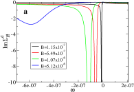
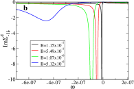
Figure S2: Imaginary part of the self-energies. a) $\Sigma^{d}_{1\uparrow}$ and b) $\Sigma^{d}_{-1\downarrow}$, close to the Fermi level, for different magnetic fields. The Anderson Hamiltonian parameters are the same as in the main text, except for $D=1.08D_{c}$.

Supplementary Note 4: Detailed comparison with experiment

In this note, we compare side by side experimental results and our theory for three sets of experiments.

Dependence of the differential conductance as the molecule is separated from the surface

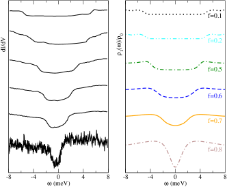
Figure S3: Raising molecule from surface. Left: experimental differential conductance as a function of voltage (taken from Fig. 2 (b) of Ref. [3]). Right: theoretical spectral density of level 1 as a function of energy, as the molecule is raised from the surface. The spectral densities plotted are the same as in Fig. 2 of the main text, where a rescaling along the vertical axis was made for a direct comparison with experimental data.

In Supplementary Fig. S3 we represent a set of experimental curves for the differential conductance $dI/dV$ taken from Ref. [3] as the molecule is raised from the surface and compare them with the corresponding spectral density of the localized states of symmetry $3z^{2}-r^{2}$ in our model. Since the experimental results are affected by a factor that decays exponentially with the distance between the tip and the surface, which is not included in our model, we have multiplied them by an arbitrary factor $f$.

In general, the shapes of experimental and theoretical curves are very similar, except for large separations (top) for which the theoretical curves are affected by the resolution of the NRG calculations and for small separations (bottom) for which some admixture of conduction states is expected to influence the conductance and is taken into account by the factor $q$ in Eq. (8) of the main text. In particular, the comparison when the molecule is on the surface is discussed below including this factor.

Differential conductance for different temperatures

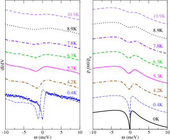
Figure S4: Temperature dependence. Left: experimental differential conductance as a function of voltage for several temperatures. Curves with different type of lines are taken from Fig. 2 (b) of Ref. [17] and data in dots ($T=0.4\,K$) is taken with permission from Fig. 1 (c) of Ref. [4]. Right: temperature dependence of the differential conductance as a function of voltage as in Fig. 3 of the main text with a vertical displacement for a better comparison with the left panel.

In Supplementary Fig. S4 we compare experiment (taken mainly from Ref. [17]) and theory for the differential conductance $dI/dV$ at different temperatures. The trend of experimental and theoretical curves is very similar. The theoretical curves have a steeper downwards slope for positive voltage, and in the experiment the maximum in $dI/dV$ for positive voltage is larger than the relative maximum for negative voltage. Both features might be related with the effect of subtraction of a background or other features of a particular experiment. At the lowest experimental temperature (0.4 K) we also show the experimental curve taken from Fig. 1 (c) of Ref. [4]. This allows the reader to grasp some experimental uncertainties.

Differential conductance for different magnetic fields

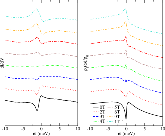
Figure S5: Magnetic field dependence. Left: experimental differential conductance as a function of voltage for several values of the magnetic field (taken from Fig. 2 (c) of Ref. [17]). Right: magnetic field dependence of the differential conductance as a function of voltage as in Fig. 4 of the main text with a vertical displacement for a better comparison with the left panel.

In Supplementary Fig. S5 we compare the experimental results for $dI/dV$ (also taken from Ref. [17]) and theory for different magnetic fields, assuming a gyromagnetic factor $g=2$, inside the range of uncertainty of values reported in the supplemental material of Refs. [3], [17]. Taking into account the features mentioned above related with experimental uncertainties, and the absence of alternative physical explanations, the agreement is very good.

Supplementary References

R. Hiraoka, E. Minamitani, R. Arafune, N. Tsukahara, S. Watanabe, M. Kawai, and N. Takagi, Single-molecule quantum dot as a Kondo simulator, Nature Commun. 8, 16012 (2017).

E. Minamitani, N. Tsukahara, D. Matsunaka, Y. Kim, N. Takagi, and M. Kawai, Symmetry-Driven Novel Kondo Effect in a Molecule, Phys. Rev. Lett. 109, 086602 (2012).

A. M. Oleš, Antiferromagnetism and correlation of electrons in transition metals, Phys. Rev. B 28, 327 (1983).

A. C. Hewson, The Kondo Problem to Heavy Fermions(Cambridge University Press, Cambridge, UK, 1997).

G. Mahan, Many-Particle Physics, Physics of Solids and Liquids (Plenum, New York, 1990).

A. Yoshimori and A. Zawadowski, Restricted Friedel sum rules and Korringa relations as consequences of conservation laws, Phys. C 15, 5241 (1982).

D. C. Langreth, Friedel Sum Rule for Anderson’s Model of Localized Impurity States, Phys. Rev. 150, 516 (1966).

J. M. Luttinger, Fermi Surface and Some Simple Equilibrium Properties of a System of Interacting Fermions, Phys. Rev. 119, 1153 (1960).

G. G. Blesio, L. O. Manuel, P. Roura-Bas, and A. A. Aligia, Topological quantum phase transition between Fermi liquid phases in an Anderson impurity model, Phys. Rev. B 98, 195435 (2018).

G. G. Blesio, L. O. Manuel, P. Roura-Bas, and A. A. Aligia, Fully compensated Kondo effect for a two-channel spin $S=1$ impurity, Phys. Rev. B 100, 075434 (2019).

O. J. Curtin, Y. Nishikawa, A. C. Hewson, and D. J. G. Crow, Fermi liquids and the Luttinger theorem, J. Phys. Commun. 2, 031001 (2018).

Y. Nishikawa, O. J. Curtin, A. C. Hewson, and D. J. G. Crow, Magnetic field induced quantum criticality and the Luttinger sum rule, Phys. Rev. B 98, 104419 (2018).

K. Seki and S. Yunoki, Topological interpretation of the Luttinger theorem, Phys. Rev. B 96, 085124 (2017).

R. A. Horn and C. R. Johnson, Matrix Analysis (Cambridge University Press, Cambridge, 2012).

K. Yang, H. Chen, Th. Pope, Y. Hu, L. Liu, D. Wang, L. Tao, W. Xiao, X. Fei, Y-Y. Zhang, H-G Luo, S. Du, T. Xiang, W. A. Hofer, and H-J. Gao, Tunable giant magnetoresistance in a single-molecule junction, Nature Commun. 10, 1038 (2019).

References

- [1] S. V. Aradhya and L. Venkataraman, Single-molecule junctions beyond electronic transport, Nature Nanotechnology 8 399 (2013).
- [2] J. C. Cuevas and E. Scheer, Molecular Electronics: An Introduction to Theory and Experiment (World Scientific, Singapore, 2010).
- [3] F. Evers, R. Korytár, S. Tewari, and J. van Ruitenbeek, Advances and challenges in single-molecule electron transport, Rev. Mod. Phys. 92, 035001 (2020).
- [4] W. Liang, M. P. Shores, M. Bockrath, J. R. Long, and H. Park, Kondo resonance in a single-molecule transistor, Nature 417, 725 (2002).
- [5] L. H. Yu, Z. K. Keane, J. W. Ciszek, L. Cheng, J. M. Tour, T. Baruah, M. R. Pederson, and D. Natelson, Kondo Resonances and Anomalous Gate Dependence in the Electrical Conductivity of Single-Molecule Transistors, Phys. Rev. Lett. 95, 256803 (2005).
- [6] M. N. Leuenberger and E. R. Mucciolo, Berry-Phase Oscillations of the Kondo Effect in Single-Molecule Magnets, Phys. Rev. Lett. 97, 126601 (2006).
- [7] E. A. Osorio, K. O’Neill, M. Wegewijs, N. Stuhr-Hansen, J. Paaske, T. Thomas Bjørnholm, and H. S. J. van der Zant, Electronic Excitations of a Single Molecule Contacted in a Three-Terminal Configuration, Nano. Lett. 7, 3336 (2007).
- [8] J. J. Parks, A. R. Champagne, G. R. Hutchison, S. Flores-Torres, H. D. Abruña, and D. C. Ralph, Tuning the Kondo Effect with a Mechanically Controllable Break Junction, Phys. Rev. Lett. 99, 026601 (2007).
- [9] N. Roch, S. Florens, V. Bouchiat, W. Wernsdorfer, and F. Balestro, Quantum phase transition in a single-molecule quantum dot, Nature 453, 633 (2008).
- [10] N. Roch, S. Florens, T. A. Costi, W. Wernsdorfer, and F. Balestro, Observation of the Underscreened Kondo Effect in a Molecular Transistor, Phys. Rev. Lett. 103, 197202 (2009).
- [11] E. A. Osorio, K. Moth-Poulsen, H. S. J. van der Zant, J. Paaske, P. Hedegård, K. Flensberg, J. Bendix, and T. Thomas Bjørnholm, Electrical Manipulation of Spin States in a Single Electrostatically Gated Transition-Metal Complex, Nano. Lett. 10, 105 (2010).
- [12] J. J. Parks, A. R. Champagne, T. A. Costi, W. W. Shum, A. N. Pasupathy, E. Neuscamman, S. Flores-Torres, P. S. Cornaglia, A. A. Aligia, C. A. Balseiro, G. K.-L. Chan, H. D. Abruña, and D. C. Ralph, Mechanical Control of Spin States in Spin-1 Molecules and the Underscreened Kondo Effect, Science 328, 1370 (2010).
- [13] S. Florens, A, Freyn, N. Roch, W. Wernsdorfer, F. Balestro, P. Roura-Bas, and A. A. Aligia, Universal transport signatures in two-electron molecular quantum dots: gate-tunable Hund’s rule, underscreened Kondo effect and quantum phase transitions, J. Phys. Condens. Matter 23, 243202 (2011), and references therein.
- [14] R. Vincent, S. Klyatskaya, M. Ruben, W. Wernsdorfer, and F. Balestro, Electronic read-out of a single nuclear spin using a molecular spin transistor, Nature (London) 488, 357 (2012).
- [15] E. Minamitani, N. Tsukahara, D. Matsunaka, Y. Kim, N. Takagi, and M. Kawai, Symmetry-Driven Novel Kondo Effect in a Molecule, Phys. Rev. Lett. 109, 086602 (2012).
- [16] B. W. Heinrich, L. Braun, J. I. Pascual, and K. J. Franke, Tuning the magnetic anisotropy of single molecules, Nano. Lett. 15, 4024 (2015).
- [17] M. Ormaza, P. Abufager, B. Verlhac, N. Bachellier, M.-L. Bocquet, N. Lorente, and L. Limot, Controlled spin switching in a metallocene molecular junction, Nature Commun. 8, 1974 (2017).
- [18] R. Hiraoka, E. Minamitani, R. Arafune, N. Tsukahara, S. Watanabe, M. Kawai, and N. Takagi, Single-molecule quantum dot as a Kondo simulator, Nature Commun. 8, 16012 (2017).
- [19] K. Yang, H. Chen, Th. Pope, Y. Hu, L. Liu, D. Wang, L. Tao, W. Xiao, X. Fei, Y-Y. Zhang, H-G Luo, S. Du, T. Xiang, W. A. Hofer, and H-J. Gao, Tunable giant magnetoresistance in a single-molecule junction, Nature Commun. 10, 1038 (2019).
- [20] Ph. Nozières and A. Blandin, Kondo effect in real metals, J. Physique 41 193 (1980).
- [21] P. Mehta, N. Andrei, P. Coleman, L. Borda, and G. Zaránd, Regular and singular Fermi-liquid fixed points in quantum impurity models, Phys. Rev. B 72, 014430 (2005).
- [22] D. E. Logan, C. J. Wright, and M. R. Galpin, Correlated electron physics in two-level quantum dots: Phase transitions, transport, and experiment, Phys. Rev. B 80, 125177 (2009).
- [23] P. S. Cornaglia, P. Roura-Bas, A. A. Aligia and C. A. Balseiro, Quantum transport through a stretched spin-1 molecule, Europhys. Lett. 93, 47005 (2011).
- [24] R. M. Potok, I. G. Rau, H. Shtrikman, Y. Oreg, and D. Goldhaber-Gordon, Observation of the two-channel Kondo effect, Nature 446, 167 (2007).
- [25] Z. Iftikhar, S. Jezouin, A. Anthore, U. Gennser, F.D. Parmentier, A. Cavanna, F. Pierre, Two-channel Kondo effect and renormalization flow with macroscopic quantum charge states, Nature 526, 233, (2015).
- [26] L. J. Zhu, S.H. Nie, P. Xiong, P. Schlottmann, and J.H. Zha, Orbital two-channel Kondo effect in epitaxial ferromagnetic L10-MnAl films, Nature Commun. 7, 10817 (2016).
- [27] G. G. Blesio, L. O. Manuel, P. Roura-Bas, and A. A. Aligia, Topological quantum phase transition between Fermi liquid phases in an Anderson impurity model, Phys. Rev. B 98, 195435 (2018).
- [28] G. G. Blesio, L. O. Manuel, P. Roura-Bas, and A. A. Aligia, Fully compensated Kondo effect for a two-channel spin impurity, Phys. Rev. B 100, 075434 (2019).
- [29] A. F. Otte, M. Ternes, K. von Bergmann, S. Loth, H. Brune, C. P. Lutz, C. F. Hirjibehedin, and A. J. Heinrich, The role of magnetic anisotropy in the Kondo effect, Nat. Phys. 4, 847 (2008).
- [30] R. Žitko, R. Peters, and T. Pruschke, Properties of anisotropic magnetic impurities on surfaces, Phys. Rev. B 78, 224404 (2008).
- [31] R. Žitko and Th. Pruschke, Many-particle effects in adsorbed magnetic atomswith easy-axis anisotropy: the case of Fe on theCuN/Cu(100) surface, New J. Phys. 12, 063040 (2010).
- [32] S. Di Napoli, A. Weichselbaum, P. Roura-Bas, A. A. Aligia, Y. Mokrousov, and S. Blügel, Non-Fermi liquid behaviour in transport through Co-doped Au chains, Phys. Rev. Lett. 110, 196402 (2013).
- [33] J. C. Oberg, M. R. Calvo, F. Delgado, M. Moro-Lagares, D. Serrate, D. Jacob, J. Fernandez-Rossier, and C. F. Hirjibehedin, Control of single-spin magnetic anisotropy by exchange coupling, Nat. Nanotechnol. 9, 64 (2013).
- [34] D. C. Langreth, Friedel Sum Rule for Anderson’s Model of Localized Impurity States, Phys. Rev. 150, 516 (1966).
- [35] A Yoshimori and A Zawadowski, Restricted Friedel sum rules and Korringa relations as consequences of conservation laws, J. Phys. C 15, 5241 (1982).
- [36] O. J. Curtin, Y. Nishikawa, A. C. Hewson, and D. J. G. Crow, Fermi liquids and the Luttinger theorem, J. Phys. Commun. 2, 031001 (2018).
- [37] Y. Nishikawa, O. J. Curtin, A. C. Hewson, and D. J. G. Crow, Magnetic field induced quantum criticality and the Luttinger sum rule, Phys. Rev. B 98, 104419 (2018).
- [38] X. Guo, Q. Zhu, L. Zhou, W. Yu, W. Lu, and W. Lian, Gate tuning and universality of Two-stage Kondo effect in single molecule transistors, Nature Commun. 12, 1566 (2021)
- [39] J. Fernández, P. Roura-Bas, A. Camjayi, and A. A. Aligia, Two-stage three-channel Kondo physics for an FePc molecule on the Au(111) surface, J. Phys.: Condens. Matter 30, 374003 (2018); Corrigendum J. Phys. Condens. Matter 31, 029501 (2018).
- [40] O. Újsághy, J. Kroha, L. Szunyogh, and A. Zawadowski, Theory of the Fano Resonance in the STM Tunneling Density of States due to a Single Kondo Impurity, Phys. Rev. Lett. 85, 2557 (2000).
- [41] A. A. Aligia and A. M. Lobos, Mirages and many-body effects in quantum corrals, J. Phys.: Condens. Matter 17, S1095 (2005).
- [42] A. Allerdt, H. Hafiz, B. Barbiellini, A. Bansil, and A. E. Feiguin, Many-body effects in porphyrin-like transition metal complexes embedded in graphene, Appl. Sci. 10, 2542 (2020).
- [43] A. C. Hewson, The Kondo Problem to Heavy Fermions (Cambridge University Press, Cambridge, UK, 1997).
- [44] R. Allub and A. A. Aligia, Ground state and magnetic susceptibility of intermediate-valence Tm impurities, Phys. Rev. B 52, 7987 (1995).
- [45] W. Hofstetter and H. Schoeller, Quantum Phase Transition in a Multilevel Dot, Phys. Rev. Lett. 88, 016803 (2001).
- [46] J. Paaske, A. Rosch, P. Wölfle, N. Mason, C. M. Markus, and J. Nygard, Nat. Phys. 2, 460 (2006).
- [47] P. Roura-Bas and A. A. Aligia, Nonequilibrium transport through a singlet-triplet Anderson impurity, Phys. Rev. B 80, 035308 (2009).
- [48] P. Roura-Bas and A. A. Aligia, Nonequilibrium dynamics of a singlet-triplet Anderson impurity near the quantum phase transition, J. Phys.: Condens. Matter 22, 025602 (2010).
- [49] While three channels participate in FePc [39] including all of them in an NRG calculation would lead to a too fast increase in the Hilbert space as a function of the iteration rendering impossible to obtain precise results.
- [50] M. Mabrouk, R. Hayn, and R. B Chaabane, Adsorption of Iron Phthalocyanine on a Au(111) Surface, Russ. J. Phys. Chem. 94, 1704 (2020).
- [51] S. Stepanow, P. S. Miedema, A. Mugarza, G. Ceballos, P. Moras, J. C. Cezar, C. Carbone, F. M. F. de Groot, and P. Gambardella, Mixed-valence behavior and strong correlation effects of metal phthalocyanines adsorbed on metals, Phys. Rev. B 83, 220401(R) (2011).
- [52] S. Kezilebieke, A. Amokrane, M. Abel, and J-P. Bucher, Hierachy of Chemical Bonding in the Synthesis of Fe-Phthalocyanine on Metal Surfaces: A Local Spectroscopy Approach, J. Phys. Chem. Lett. 5, 3175 (2014).
- [53] L. Gao, W. Ji, Y. B. Hu, Z. H. Cheng, Z. T. Deng, Q. Liu, N. Jiang, X. Lin, W. Guo, S. X. Du, W. A. Hofer, X. C. Xie, and H.-J. Gao, Site-Specific Kondo Effect at Ambient Temperatures in Iron-Based Molecules, Phys. Rev. Lett. 99, 106402 (2007).
- [54] A. Mugarza, R. Robles, C. Krull, R. Korytár, N. Lorente, and P. Gambardella, Electronic and magnetic properties of molecule-metal interfaces: Transition-metal phthalocyanines adsorbed on Ag(100) Phys. Rev. B 85, 155437 (2012).
- [55] D. Jacob, M. Soriano, and J. J. Palacios, Kondo effect and spin quenching in high-spin molecules on metal substrates, Phys. Rev. B 88, 134417 (2013).
- [56] J. Kügel, M. Karolak, J. Senkpiel, P-J. Hsu, G. Sangiovanni, and M. Bode, Relevance of Hybridization and Filling of 3d Orbitals for the Kondo Effect in Transition Metal Phthalocyanines, Nano Lett. 14, 3895 (2014).
- [57] J. Kügel, M. Karolak, A. Krönlein, J. Senkpiel, P. Hsu, G. Sangiovanni, and M. Bode, State identification and tunable Kondo effect of MnPc on Ag(001), Phys. Rev. B 91, 235130 (2015).
- [58] A. Valli, M. Bahlke, A. Kowalski, M. Karolak, C. Herrmann, and G. Sangiovanni, Kondo screening in Co adatoms with full Coulomb interaction, Phys. Rev. Research 2, 033432 (2020).
- [59] J. R. Taylor, Scattering Theory, John Wiley & Sons, New York, 1972.
- [60] J. Friedel, XIV. The distribution of electrons round impurities in monovalent metals, Philos. Mag. 43, 153 (1952).
- [61] J. M. Luttinger, Fermi Surface and Some Simple Equilibrium Properties of a System of Interacting Fermions, Phys. Rev. 119, 1153 (1960).
- [62] J. S. Langer and V. Ambegaokar, Friedel Sum Rule for a System of Interacting Electrons, Phys. Rev. 121, 1090 (1961).
- [63] H. Shiba, The Korringa Relation for the Impurity Nuclear Spin-Lattice Relaxation in Dilute Kondo Alloys, Progress of Theoretical Physics, 54, 967 (1975).
- [64] M. S. Tacca, T. Jacob, and E. C. Goldberg, Surface states influence in the conductance spectra of Co adsorbed on Cu(111), Phys. Rev. B 103, 245419 (2021).
- [65] W. A. Harrison, Electron Structure and the Properties of Solids (Freeman, San Francisco, 1980).
- [66] R. Bulla, T. Costi and T. Pruschke, The numerical renormalization group method for quantum impurity systems, Rev. Mod. Phys. 80, 395 (2008).
- [67] D.-J. Choi, S. Guissart, M. Ormaza, N. Bachellier, O. Bengone, P. Simon, and L. Limot, Kondo Resonance of a Co Atom Exchange Coupled to a Ferromagnetic Tip, Nano Lett. 16, 6298 (2016).
- [68] D.-J. Choi, P. Abufager, L. Limot, and N. Lorente, From tunneling to contact in a magnetic atom: The non-equilibrium Kondo effect, J. Phys. Chem. 146, 092309 (2017).
- [69] D. Pérez Daroca, P. Roura-Bas, and A. A. Aligia, Relation between width of zero-bias anomaly and Kondo temperature in transport measurements through correlated quantum dots: Effect of asymmetric coupling to the leads, Phys. Rev. B 98, 245406 (2018).
- [70] J. Fernández, P. Roura-Bas, and A. A. Aligia, Theory of Differential Conductance of Co on Cu(111) Including Co s and d Orbitals, and Surface and Bulk Cu States Phys. Rev. Lett. 126, 046801 (2021).
- [71] R. Žitko, Kondo resonance lineshape of magnetic adatoms on decoupling layers, Phys. Rev. B 84, 195116 (2011).
- [72] N. Tsukahara, S. Shiraki, S. Itou, N. Ohta, N. Takagi, and M. Kawai, Evolution of Kondo Resonance from a Single Impurity Molecule to the Two-Dimensional Lattice, Phys. Rev. Lett. 106, 187201 (2011).
- [73] R. Žitko and T. Pruschke, Energy resolution and discretization artifacts in the numerical renormalization group, Phys. Rev. B 79, 085106 (2009).
- [74] NRG Ljubljana, https://github.com/rokzitko/nrgljubljana and http://nrgljubljana.ijs.si/.
- [75] K. G. Wilson, The renormalization group: Critical phenomena and the Kondo problem, Rev. Mod. Phys. 47, 773 (1975).
- [76] R. Peters, Th. Pruschke, and F. B. Anders, A numerical renormalization group approach to Green’s functions for quantum impurity models, Phys. Rev. B 74, 245114 (2006).
- [77] R. Bulla, A. C. Hewson, and Th. Pruschke, Numerical renormalization group calculations for the self-energy of the impurity Anderson model, J. Phys.: Condens. Matter 10, 8365 (1998).