Bayesian Optimisation for Constrained Problems

Abstract

Many real-world optimisation problems such as hyperparameter tuning in machine learning or simulation-based optimisation can be formulated as expensive-to-evaluate black-box functions. A popular approach to tackle such problems is Bayesian optimisation (BO), which builds a response surface model based on the data collected so far, and uses the mean and uncertainty predicted by the model to decide what information to collect next. In this paper, we propose a novel variant of the well-known Knowledge Gradient acquisition function that allows it to handle constraints. We empirically compare the new algorithm with four other state-of-the-art constrained Bayesian optimisation algorithms and demonstrate its superior performance. We also prove theoretical convergence in the infinite budget limit.

1 Introduction

Expensive black-box constrained optimisation problems appear in many fields where the possible number of evaluations is limited. Examples include hyperparameter tuning, where the objective is to minimise the validation error of a machine learning algorithm (Hernández-Lobato et al., 2016), the optimisation of the control policy of a robot under performance and safety constraints (Berkenkamp et al., 2016), or engineering design optimisation (Forrester et al., 2008).

For such applications, Bayesian optimisation (BO) has shown to be a powerful and efficient tool. After collecting some initial data, BO constructs a surrogate model, usually a Gaussian process (GP). Then it iteratively uses an acquisition function to decide what data should be collected next. The Gaussian process model is updated with the new sample information and the process is repeated until the available budget of evaluations has been consumed. Most BO approaches assume unconstrained or box-constrained problems.

In this paper, we make the following contributions.

1. We develop a new variant of the Knowledge Gradient acquisition function, called constrained Knowledge Gradient (cKG), capable of handling constraints.

2. We show how cKG can be efficiently computed.

3. We prove that cKG converges to the optimal solution in the limit.

4. We apply our proposed approach to a variety of test problems and show that cKG outperforms other available BO approaches for constrained problems.

We start with an overview of related work in Section 2, followed by a formal definition of the problem in Section 3. Section 4 explains the statistical models, shows the suggested sampling procedure, outlines its theoretical properties and computation. We perform numerical experiments in Section 5. Finally, the paper concludes with a summary and some suggestions for future work in Section 6.

2 Literature Review

Bayesian optimisation (BO) has gained wide popularity, especially for problems involving expensive black-box functions, for a comprehensive introduction see Frazier (2018) and Shahriari et al. (2016). Although most work has focused on unconstrained problems, some extensions to constrained optimisation problems exist.

Many of the approaches are based on the famous Expected Improvement (EI) acquisition function (Jones et al., 1998). Schonlau et al. (1998) and Gardner et al. (2014) extended EI to constrained EI (cEI) by computing the expected improvement of a point $x$ over the best feasible point and multiplying it by its probability of being feasible. This relies on the assumption that the objective function and constraints are independent, and that the decision maker is risk neutral. Bagheri et al. (2017) proposed a modified combination of probability of feasibility with EI that makes it easier to find solutions on the feasibility boundary.

Several extensions to EI have also been proposed for noisy problems. Letham et al. (2017) extended Expected Improvement to noisy observations (NEI) and noisy constraints by iterating the expectation over possible posterior distributions. For noise-free observations, their approach reduces to the original cEI. Other methods rely on relaxing the constraints instead of modifying the infill criteria, Gramacy et al. (2016) proposed an augmented Lagrangian approach that includes constraints as penalties in the objective function. Picheny et al. (2016) refined the previous approach by introducing slack variables and achieve better performance on equality constraints.

The Knowledge Gradient (KG) policy (Scott et al. (2011)) is another myopic acquisition function that aims to maximise the new predicted optimal performance after one new sample, and can be directly applied to either deterministic or noisy functions. Chen et al. (2021) recently proposed an extension of KG to constraints by multiplying any new sampling location by its probability of feasibility. These approaches consider noise in the observations and constraints but they only use the current feasibility information. In contrast, Lam and Willcox (2017) consider deterministic problems and proposed a lookahead approach for the value of feasibility information, selecting the next evaluation in order to maximise the long-term feasible increase of the objective function. This was formulated using dynamic programming where each simulated step gives a reward following cEI.

Other acquisition functions not based on EI have also been considered to tackle constraints. Hernandez-Lobato et al. (2016) extended Predictive Entropy Search (Henrnandez-Lobato et al., 2014) to constraints. This acquisition criterion involves computing the expected entropy reduction of the global solution to the constrained optimization problem. Eriksson et al. (2019) extended Thompson sampling for constrained optimisation and also proposed a trust region to limit the search to locations close to the global optimum. Picheny (2014) proposed an optimisation strategy where the benefit of a new sample is measured by the reduction of the expected volume of the excursion set which provides a measure of uncertainty on the minimiser location where constraints can be incorporated in the formulation by a solution’s probability of being feasible. However this can only be computed approximately using numerical integration. Antonio (2019) proposed a two-stage approach where the feasible region is estimated during the first stage by a support-vector classifier, then the second stage uses the estimated boundaries and maximises the objective function value using the Upper Confidence Bound (UCB) as acquisition function.

3 Problem Definition

We want to find the optimizer $x^{*}$ of a black-box function $f:\mathbb{X}\rightarrow\mathbb{R}$ with constraints $c_{k}:\mathbb{X}\rightarrow\mathbb{R}$, i.e.,

$$\begin{split}x^{*}=\operatorname*{arg\,max}_{x\in\mathbb{X}}f(x)\end{split}$$ (1)

$$\begin{split}\mbox{s.t.}\text{ }&c_{k}(x)\leq 0\text{ },k=1,\dots,K\end{split}$$ (2)

The objective function $f$ takes as arguments a design vector $x\in\mathbb{X}\subset\mathbb{R}^{d}$ and returns an observation corrupted by noise $y=f(x)+\epsilon$, where $\epsilon\sim N(0,\sigma^{2}_{\epsilon})$, and a vector of constraint values $\mathbf{c}=[c_{1}(x),\dots,c_{K}(x)]$.

There is a total budget of $B$ samples that can be spent. After consuming the budget, a recommended design, $x_{r}$, is returned to the user and its quality is determined by the difference in objective function to the best solution $x^{*}$ given that $x_{r}$ is feasible, i.e. $x\in F=\{x|c_{k}(x)\leq 0\quad\forall k\in[1\ldots K]\}$. If $x_{r}$ is not feasible then there is a penalty $M$ for not having a feasible solution. Therefore, the quality of a solution may be measured as an Opportunity Cost (OC) to be minimised,

$$OC(x_{r})=\begin{cases}f(x^{*})-f(x_{r})&\text{if $x_{r}\in F$}\\ f(x^{*})-M&\text{otherwise}\end{cases}$$ (3)

Without loss of generality we assume a penalty $M=0$. However, $M$ may be set by using the minimum GP estimate of the objective function in the design space (Letham et al., 2017).

4 The cKG Algorithm

4.1 Statistical Model

Let us denote all $n$ design vectors sampled so far as $X=\{x_{i}\}_{i=1}^{n}$ and the training data from the collection of objective function observations , $\mathscr{D}_{f}=\{(x,y)\}_{i=1}^{n}$, and constraints,$\mathscr{D}_{c}=\{(x,\mathbf{c})\}_{i=1}^{n}$. We model the objective function observations as a Gaussian process (GP) which is fully specified by a mean function $\mu_{y}^{n}(x)=\mathbb{E}[y(x)|\mathscr{D}_{f}]$ and its covariance $\text{Cov}\,[y(x),y(x^{\prime})|\mathscr{D}_{f}]$,

$$\begin{split}\mathbb{E}[y(x)|\mathscr{D}_{f}]&=\mu_{y}^{n}(x)\\ &=\mu_{y}^{0}(x)-k_{y}^{0}(x,X)(k_{y}^{0}(X,X)+I\sigma^{2}_{\epsilon})^{-1}(Y-\mu_{y}^{0}(X))\end{split}$$ (4)

$$\begin{split}\text{Cov}\,[y(x),y(x^{\prime})|\mathscr{D}_{f}]&=k_{y}^{n}(x,x^{\prime})\\ &=k_{y}^{0}(x,x^{\prime})-k_{y}^{0}(x,X)(k_{y}^{0}(X^{n},X^{n})+I\sigma^{2}_{\epsilon})^{-1}k_{y}^{0}(X,x^{\prime})).\end{split}$$ (5)

Similarly, each constraint is modelled as an independent GP over the training data $\mathscr{D}_{c}$ defined by a constraint mean function $\mu_{k}^{n}(x)=\mathbb{E}[c_{k}(x)|\mathscr{D}_{c}]$ and covariance $\text{Cov}\,[c_{k}(x),c_{k}(x^{\prime})|\mathscr{D}_{c}]$. The prior mean is typically set to zero and the kernel allows the user to encode known properties such as smoothness and periodicity. We use the popular squared exponential kernel that assumes $f$ and $\mathbf{c}$ are smooth functions, i.e., nearby $x$ have similar outputs while widely separated points have unrelated outputs. Further details can be found in Rasmussen and Williams (2006).

4.2 Recommended Solution

At the end of the algorithm we must recommend a final feasible design vector, $x_{r}$. Assuming a risk-neutral user, the utility of a design vector is the expected objective performance , $\mu_{y}^{n}(x)$, if feasible, and zero $(M)$ if infeasible. Therefore, if the constraints and objective are independent, a recommended solution $x_{r}$ may be obtained by

$$x_{r}=\operatorname*{arg\,max}_{x\in\mathbb{X}}{\mu_{y}^{B}(x)\mathbb{P}[\mathbf{c}^{B}(x)\leq 0]},$$ (6)

where $\mathbb{P}[\mathbf{c}^{B}(x)\leq 0]$ is the probability of feasibility of a design $x$. Following Gardner et al. (2014), we assume independent constraints, such that $\mathbb{P}[\mathbf{c}^{B}(x)\leq 0|\mathscr{D}_{c}]=\prod_{k=1}^{K}\mathbb{P}[c^{B}_{k}(x)\leq 0|\mathscr{D}_{c}]$. Each term $\mathbb{P}[c_{k}(x)\leq 0|\mathscr{D}_{c}]$ can be evaluated by a univariate Gaussian cumulative distribution. In the remainder of this work we denote the probability of feasibility as $\text{PF}^{n}(x)$.

4.3 Acquisition Function

We aim for an acquisition function that quantifies the value of the objective function and constraint information we would gain from a given sampling decision. Note that obtaining feasibility information does not immediately translate to better expected objective performance but rather more accurate feasibility information where more updated feasibility information may change our current beliefs about where $x_{r}$ is located. Therefore, to quantify the benefit of a design vector, we first find the recommended design given by the sampled trained data $\mathscr{D}_{c}$ and $\mathscr{D}_{f}$ as,

$$\begin{split}x^{n}_{r}=\operatorname*{arg\,max}_{x\in\mathbb{X}}{\mu_{y}^{n}(x)\text{PF}^{n}(x)}.\end{split}$$ (7)

A sensible compromise between the current step $n$ and the one-step lookahead estimated performance is offered by augmenting the training data by the sampling decision $x^{n+1}$ with its respective constraint and objective observations as $\mathscr{D}_{c}\cup\{x^{n+1},\mathbf{c}^{n+1}\}$ and $\mathscr{D}_{f}\cup\{x^{n+1},y^{n+1}\}$. The difference in performance between the current recommended design and the new best performance presents an acquisition function for a design $x$,

$$\begin{split}\text{cKG}(x)&=\mathbb{E}[\max_{x^{\prime}\in\mathbb{X}}\big{\{}\mu_{y}^{n+1}(x^{\prime})\text{PF}^{n+1}(x^{\prime})\big{\}}-\mu_{y}^{n+1}(x^{n}_{r})\text{PF}^{n+1}(x^{n}_{r})|x^{n+1}=x].\end{split}$$ (8)

Eqn. 8 is positive for all the design space and $\mu_{y}^{n+1}(x^{n}_{r})$ may be marginalised over $y^{n+1}$, such that

$$\begin{split}\text{cKG}(x)&=\mathbb{E}[\max_{x^{\prime}\in\mathbb{X}}\big{\{}\mu_{y}^{n+1}(x^{\prime})\text{PF}^{n+1}(x^{\prime})\big{\}}-\mu_{y}^{n}(x^{n}_{r})\text{PF}^{n+1}(x^{n}_{r})|x^{n+1}=x].\end{split}$$ (9)

This acquisition function quantifies the benefit of a design vector and takes into account the change in the current performance value when more feasibility information is available. Also, when constraints are not considered, the formulation reduces to standard KG (Scott et al., 2011). Theoretical guarantees can be proven for cKG. This policy ensures in a finite search space $\mathbb{X}$, with an infinite sampling budget all points will be sampled infinitely often which ensures learning the true expected observation (Theorem 1). Also, in the limit, cKG will find the true optimal solution $x^{*}$ (Theorem 2).

4.4 Efficient Acquisition Function Computation

Obtaining a closed-form expression for cKG is not possible but as we show below, it can still be computed efficiently. Pearce et al. (2020) proposed an efficient one-step-lookahead computation that consists of obtaining high value points for different realisations of the posterior GP mean given a sample design vector . Those discrete design vectors can then be used as a discretisation in the design space for which a closed-form solution exists. This approach is both computationally efficient and scalable with the number of design vector dimensions, thus we adapt this method to our constrained problem.

We first convert $\mu_{y}^{n+1}(x)$ to quantities that can be computed in the current step $n$ through the parametrisation trick (Scott et al., 2011) as $\mu_{y}^{n+1}(x)=\mu_{y}^{n}(x)+\tilde{\sigma_{y}}(x,x^{n+1})Z_{y}$ where $Z_{y}\sim N(0,1)$. The deterministic function $\tilde{\sigma}^{n}(x,x^{n+1})$ represents the standard deviation of $\mu_{y}^{n+1}(x)$ parametrised by $x^{n+1}$ and given by, $\tilde{\sigma}^{n}(x,x^{n+1})=\frac{k^{n}(x,x^{n+1})}{\sqrt{k^{n}(x^{n+1},x^{n+1})+\sigma^{2}_{\epsilon}}}$.

Similarly, we may apply the parametrisation trick to the posterior means and variances of the constraints, i.e, $\mu_{k}^{n+1}(x)=\mu_{k}^{n}(x)+\tilde{\sigma_{k}}(x,x^{n+1})Z_{k}$ and $k^{n+1}_{k}(x,x)=k^{n}_{k}(x,x)-\tilde{\sigma_{k}}^{2}(x,x^{n+1})$, where $Z_{k}\sim N(0,1)$ for $k=1,\dots,K$. Now, the probability of feasibility is also parametrised by $x^{n+1}$ and all the stochasticity is determined by $\mathbf{Z}_{c}=[Z_{1},\dots,Z_{K}]$. By plugging these parametrisations into Eqn. 9, we change our initial problem to variables that can be estimated in the current step where the stochasticity is given by standard normally distributed random variables for both constraints and the objective,

$$\begin{split}\text{cKG}(x)&=\mathbb{E}\Bigg{[}\overbrace{\max_{x^{\prime}\in\mathbb{X}}\big{\{}\big{[}\mu_{y}^{n}(x^{\prime})+\tilde{\sigma}_{y}(x^{\prime},x^{n+1})Z_{y}\big{]}\text{PF}^{n+1}(x^{\prime};x^{n+1},\mathbf{Z}_{c})}^{\text{Inner Optimisation $n+1$}}\big{\}}\end{split}$$

$$\begin{split}&-\mu_{y}^{n}(x_{r})\text{PF}^{n+1}(x^{n}_{r};x^{n+1},\mathbf{Z}_{c})|x^{n+1}=x\Bigg{]}.\end{split}$$ (10)

To solve the above expectation we first find $x^{n}_{r}$ according to Eqn. 7 using a continuous numerical optimiser. Then, given a design $x^{n+1}$, we generate $n_{y}$ values from $Z_{y}$ and $n_{c}$ values from $\mathbf{Z_{c}}$ where the inner optimisation problems in Eqn. 10 is solved by a continuous numerical optimiser for all $n_{z}=n_{c}*n_{y}$ values. Each solution found by the optimiser, $x_{j}^{*}$, represents a peak location, and together they determine a discretisation $X_{d}=\{x_{1}^{*},\dots,x_{n_{z}}^{*}\}$. Finally, Eqn. 10 can be solved in closed-form where now the inner optimisation problems are computed over the discrete set $X_{d}$. Conditioned on $\mathbf{Z}_{c}$, the above expectation can be seen as marginalising the standard discrete KG (Scott et al., 2011) over the constraint uncertainty where $\mu_{y}^{n}(x)$ and $\tilde{\sigma_{y}}(x,x^{n+1})$ is penalised by the (deterministic) function $\text{PF}^{n+1}(x;x^{n+1},\mathbf{Z}_{c})$. Therefore, if we denote each standard KG computation as $\text{KG}_{d}(x^{n+1}=x;\mathbf{Z}_{c})$ we may compute the overall expectation by a Monte-Carlo approximation,

$$\begin{split}\text{cKG}(x)&=\frac{1}{n_{c}}\sum_{m=1}^{n_{c}}\text{KG}_{d}(x^{n+1}=x;\mathbf{Z}^{m}_{c}).\end{split}$$ (11)

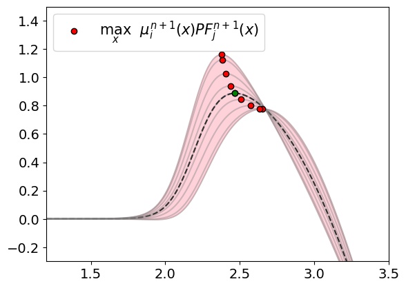
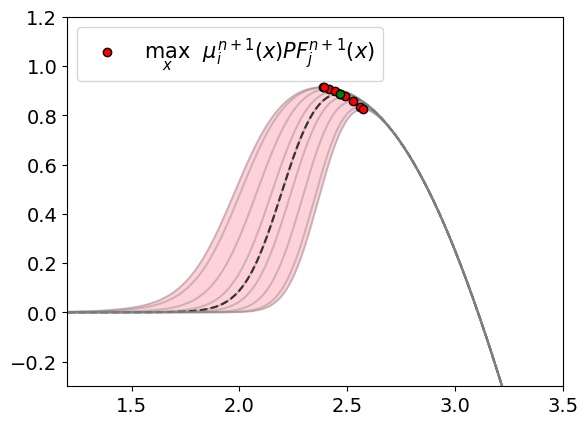
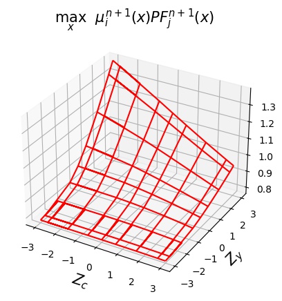
(a)	(b)	(c)

Figure 1: (a) Given $\mathbf{Z_{c}}=0$, current GP mean (dotted grey) and maximum (green dot) where changing $Z_{y}$ produces a different realisation and a new maximum (red dots). (b) Given $Z_{y}=0$, different values of $\mathbf{Z}_{c}$ produces a new maximum according to the probability of feasibility. (c) shows the surface of the maximum posterior over the discrete set for all combinations of $\mathbf{Z}_{c}$ and $Z_{y}$.

Fig. 1 shows the influence of a sample $x^{n+1}$ on computing the expectation at $n+1$ in Eqn. 10. More specifically, if we fix $\mathbf{Z}_{c}$, Fig. 1 (a) shows how the current GP mean (dotted grey) and maximum (green dot) could change according to $Z_{y}$ where each different realisation presents a new maximum (red dots). However, if we fix $Z_{y}$, Fig. 1 (b) shows how the maximum of the GP mean may change according to the probability of feasibility. Fig. 1 (c) shows the surface of the maximum locations for all combinations of $\mathbf{Z}_{c}$ and $Z_{y}$.

4.5 Overall Algorithm

Fig. 2 shows iterations of cKG. Fig. 2 (a) shows an objective function (blue) and a constraint (purple) with negative constraint values representing feasible solutions. The aim is to find the best feasible solution at $x^{*}=6.25$, see also Fig. 2 (b). Then, GPs are built based on initial samples, and (c) shows the posterior utility (dotted line, posterior $y$ times probability of feasibility). Then, the next design vector is obtained my maximising cKG. Finally, after the budget of $B$ samples has been allocated sequentially, a final recommendation $x_{r}$ is selected according to Eqn. 7 where $x_{r}$ (orange dot) ends up being very close to the true best $x^{*}$ (green dot). Notice that cKG aims at improving the maximal posterior mean, not the quality at the sampled solution, and thus often tends to sample the neighborhood of $x^{*}$ instead of the actual best design vector location.

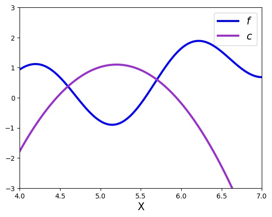
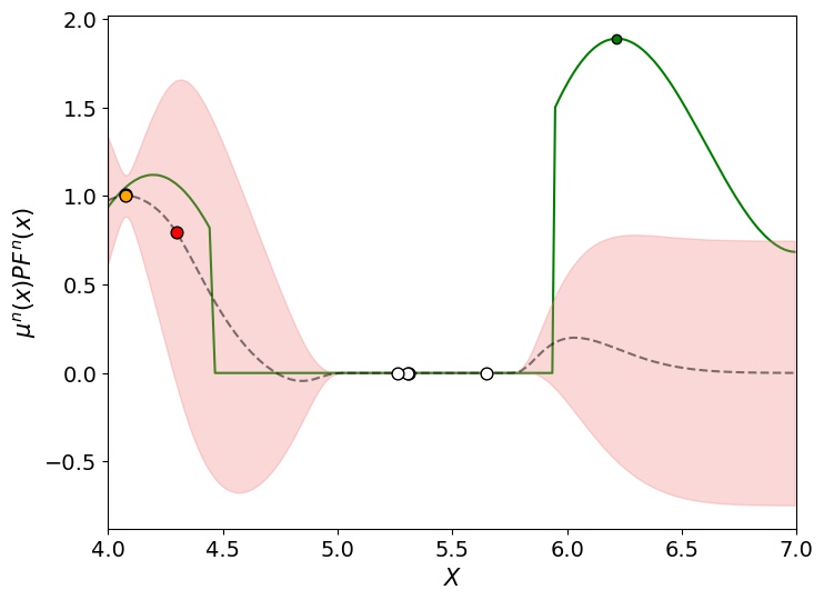
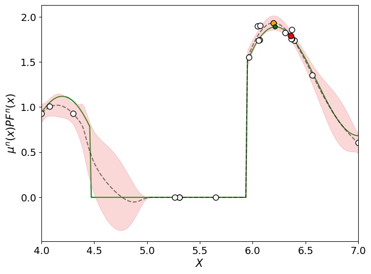
(a)	(c)	(e)
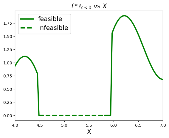
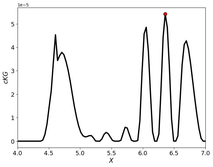
(b)	(d)	(f)

Figure 2: (a) objective function and constraint where constraint values less than zero are feasible. (b) Feasible and infeasible regions with its corresponding values. (c) Initial design allocation where a model is built using a GP for the objective function penalised by the probability of feasibility using a GP for the constraints. (d) and (f) show the next sample decision (red dot) according to cKG using the fitted models. (e) shows the samples taken during the entire optimisation run (white dots) with the recommended design (orange dot) coinciding with the true best design vector (green dot).

cKG is outlined in Algorithm 2. On Line 1, the algorithm begins by fitting a Gaussian process model to the initial training data $\mathscr{D}_{f}$ and $\mathscr{D}_{c}$ obtained using a Latin hypercube (LHS) ‘space-filling’ experimental design. After initialisation, the algorithm continues in an optimisation loop until the budget $B$ has been consumed. In each iteration, we sample a new design vector $x^{n+1}$ according to cKG, as defined in Algorithm 1 (Line 2). The design vector that maximises cKG determines the sample $(x,y)^{n+1}$ and $(x,\mathbf{c})^{n+1}$. The point is added to the training data $\mathscr{D}_{f}$ and $\mathscr{D}_{c}$ and each Gaussian process model is updated (Line 5). Finally, cKG recommends a design vector according to Eqn. 4.2 (Line 7). More implementation details may be found in Appendix D.

Input: Sample $x^{n+1}$, size of Monte-Carlo discretisations $n_{c}$ and $n_{y}$

0. Initialise discretisation $X^{0}_{d}=\{\}$ and set $n_{z}=n_{c}n_{y}$

1. Compute $x^{n}_{r}=\operatorname*{arg\,max}_{x\in\mathbb{X}}{\mu_{y}^{n}(x)\text{PF}^{n}(x)}$

2. for j in [1, …, $n_{z}$] :

3.     Generate $Z^{j}_{y},Z^{j}_{1},\dots,Z^{j}_{K}\sim N(0,1)$

4.     Compute $x_{j}^{*}=\max_{x\in X_{d}}\big{\{}\big{[}\mu_{y}^{n}(x)+\tilde{\sigma_{y}}(x,x^{n+1})Z^{j}_{y}\big{]}\text{PF}^{n+1}(x;x^{n+1},\mathbf{Z}^{j}_{c})\big{\}}$

5.     Update discretisation $X^{j}_{d}=X^{j-1}_{d}\cup\{x_{j}^{*}\}$

6. for m in [1, …, $n_{c}$] :

7.     Compute $\text{KG}_{d}(x^{n+1}=x;\mathbf{Z}^{m}_{c})$ using $X_{d}$

8. Compute Monte-Carlo estimation $\frac{1}{n_{c}}\sum_{m=1}^{n_{c}}\text{KG}_{d}(x^{n+1};\mathbf{Z}^{m}_{c})$

9. Return: $\text{cKG}(x^{n+1})$

Algorithm 1 cKG computation.

Input: black-box function $f:X\to\mathbb{R}$, constraints $c_{k}:X\to\mathbb{R}$, size of Monte-Carlo $n_{c}$ and $n_{y}$

0. Collect initial simulation data, $\mathscr{D}_{f}$,$\mathscr{D}_{c}$, and fit an independent Gaussian process for each constraint and the black-box function.

1. While $b$ < B do:

2.      Compute $x^{n+1}=\arg\max_{x\in X}\text{cKG}(x,n_{z},M)$.

3.      Update $\mathscr{D}_{f}$, with sample $\{(x,y)^{n+1}\}$

4.      Update $\mathscr{D}_{c}$, with sample $\{(x,\mathbf{c})^{n+1}\}$

5.      Fit a Gaussian process to $\mathscr{D}_{f}$ and $\mathscr{D}_{c}$

6.      Update budget consumed, $b\leftarrow b+1$

7. Return: Recommend solution, $x_{r}=\arg\max_{x\in\mathbb{X}}\{\mu_{y}^{B}(x)\text{PF}^{B}(x)\}$

Algorithm 2 cKG Overall Algorithm. The algorithm starts with an initialization phase to collect preliminary data, then, proceeds to a sequential phase.

5 Experiments

In this section, we compare cKG against a variety of well-known acquisition functions that can deal with constraints, including: constrained Expected Improvement (cEI) by Gardner et al. (2014), expected improvement to noisy observations (NEI) by Letham et al. (2017), Predictive Entropy Search with constraints (PESC) by Hernandez-Lobato et al. (2016), Thompson sampling for constrained optimisation (cTS) by Eriksson et al. (2019) and a recently proposed constrained KG algorithm (Chen et al., 2021) which we call penalised KG (pKG) to distinguish it from our proposed formulation (further details on the benchmark algorithms can be found in Appendix C).

We used implementations of cEI and NEI available in BoTorch (Balandat et al., 2020). For PESC, only the Spearmint optimisation package provided an available implementation of the algorithm that included constraints. The remaining algorithms have been re-implemented from scratch and can be accessed through github.

For all test problems, we fit an independent Gaussian process for each constraint $c_{k}$ and the black-box objective function $y$ with an initial design of size $10$ for the synthetic test functions and $20$ for the MNIST experiment, both chosen by Latin Hypercube Sampling. Also, for each Gaussian process, an RBF kernel is assumed with hyperparameters tuned by maximum likelihood, including the noise $\sigma^{2}_{\epsilon}$ in case of noisy problems.

5.1 Synthetic Tests

We test the algorithms on three different constrained synthetic problems: Mistery function, Test function 2, and New Branin from Sasena (2002). Each function was tested with and without a noise level $\sigma_{\epsilon}^{2}=1$ for the objective value (the constraint values were assumed to be deterministic). All synthetic test results were averaged over 30 replications and generated using a computing cluster. Further details of each function can be found in Appendix A.

Fig. 3 shows the results of these experiments. Fig. 3 (top row) depicts a contour plot of each objective function over its feasible area. The location of the optimum is highlighted by a green cross. Mistery and New Branin both have a single non-linear constraint whereas the infeasible area in Test function 2 is the result of a combination of 3 different constraints. Fig. 3 (middle row) shows the convergence of the opportunity cost over the number of iterations, for the case without noise. As can be seen, cKG outperforms all benchmark approaches on the Branin and Mistery function, with cEI second best. On Test Function 2, pKG converges to the same quality as cKG, with the other methods performing much worse. Overall cKG is the only method that consistently yields superior performance across all three test problems. Fig. 3 (bottom row) shows the performance when observations are corrupted by noise. Since cEI was designed for deterministic problems, it was replaced by the more general NEI for the noisy problems. Not surprisingly, in all cases the performance of the different considered approaches deteriorated compared to the deterministic setting. The difference between cKG and the other methods is even more apparent, with no method coming close to cKG’s performance on any of the benchmarks. This shows that cKG is particularly capable of handling noisy constrained optimisation problems.

Branin	Mistery	Test Function 2

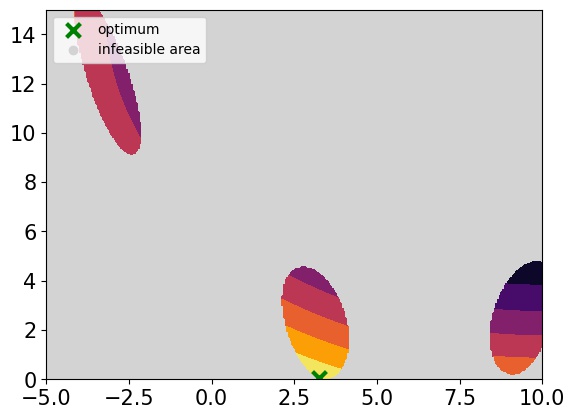
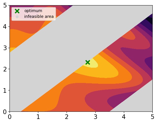
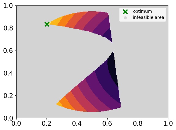
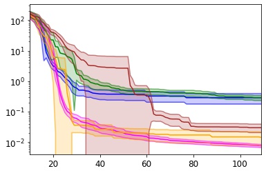
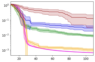
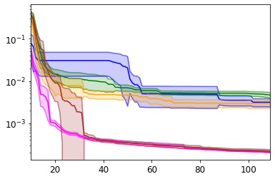
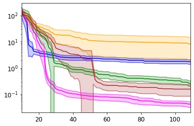
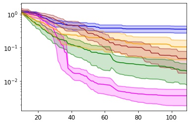
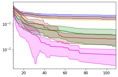
Figure 3: (top row) shows the feasible and infeasible regions of the considered synthetic functions. (middle row) and (bottom row) show the mean and 95% CI for the OC over iterations for $\sigma_{\epsilon}^{2}=0$ and $\sigma_{\epsilon}^{2}=1$, respectively.

5.2 Tuning a Fast Fully Connected Neural Network

For this experiment we aim to tune the hyperparameters of a fully connected neural network subject to a limit on the prediction time of 1 ms. The design space consists of 9 dimensions comprising the optimiser parameters and the number of neurons on each level, details of the neural network architecture may be found in Appendix B. The prediction time is computed as the average time of 3000 predictions for minibatches of size 250. The network is trained on the MNIST digit classification task using tensorflow and the objective to be minimised is the classification error rate on a validation set. Each recommended design is evaluated 20 times to compute a "ground-truth" validation error. All results were averaged over 20 replications and generated using a 20-core Intel(R) Xeon(R) Gold 6230 processor.

Fig. 4 shows that cKG yields the highest validation accuracy compared to the other considered benchmark methods. TS and pKG also perform well, which is consistent with the synthetic experiments.

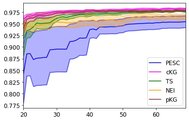
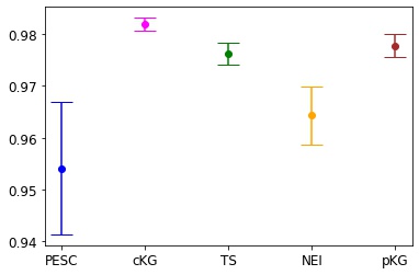
(a)	(b)

Figure 4: (a) Mean and 95% CI for the "ground-truth" validation accuracy over iterations. (b) Mean and 95% CI for the "ground-truth score" after 50 iterations.

6 Conclusion

For the problem of constrained Bayesian optimisation, we proposed a new variant of the well-known Knowledge Gradient acquisition function, constrained Knowledge Gradient (cKG), that is capable of handling constraints and noise. We show that cKG can be efficiently computed by adapting an approach proposed in Pearce et al. (2020) which is a hybrid between discretisation and Monte-Carlo approximation that allows to leverage the benefits of fast computations of the discrete design space and the scalability of continuous Monte-Carlo sampling. We prove that the algorithm will find the true optimum in the limit. Finally, we empirically demonstrate the effectiveness of the proposed approach on several test problems. cKG consistently and significantly outperformed all benchmark algorithms on all test problems, with a particularly large improvement under noisy problem settings.

Despite the excellent results, the study has some limitations that should be addressed in future work. First, while cKG should also work well with stochastic constraints, all the test problems considered here had a deterministic constraint function. Second, we have set the reward for an infeasible solution ($M$) to zero. A further study on the influence of this value may be interesting. Third, as most Bayesian optimisation algorithms, we assume the noise in the quality measure to be homoscedastic. Perhaps ideas from Stochastic Kriging can be used to relax this. Finally, we assume that an evaluation of a solution returns simultaneously its quality as well as its constraint value. In practice, it may be possible to evaluate quality and feasibility independently.

Appendix A Synthetic Test Functions

The following subsections describe the synthetic test functions used for the empirical comparison (Sasena, 2002).

A.1 Mystery Function

$$\min f(x)=2+0.01(x_{2}-x_{1}^{2})^{2}+(1-x_{1})^{2}+2*(2-x_{2})^{2}+7\text{sin}(0.5x_{1})\text{sin}(0.7x_{1}x_{2})$$

subject to

$$-\text{sin}(x_{1}-x_{2}-\frac{\pi}{8})\leq 0$$

$$x_{i}\in[0,5],\forall i=1,2$$

A.2 New Branin Function

$$\min f(x)=-(x_{1}-10)^{2}-(x_{2}-15)^{2}$$

subject to

$$\bigg{(}x_{2}-\frac{5.1}{4\pi^{2}}x_{1}^{2}+\frac{5}{\pi}x_{1}-6\bigg{)}^{2}+10\bigg{(}1-\frac{1}{8\pi}\bigg{)}\text{cos}(x_{1})+5\leq 0$$

$$x_{1}\in[-5,10]$$

$$x_{2}\in[0,15]$$

A.3 Test Function 2

$$\min f(x)=-(x_{1}-1)^{2}-(x_{2}-0.5)^{2}$$

subject to

$$(x_{1}-3)^{2}+(x_{2}+2)^{2}-12\leq 0$$

$$10x_{1}+x_{2}-7\leq 0$$

$$(x_{1}-0.5)^{2}+(x_{2}-0.5)^{2}-0.2\leq 0$$

$$x_{i}\in[0,1]\forall i=1,2$$

Appendix B MNIST Hyperparameter Experiment

Design Space:

• learning_rate $\in[0.0001,0.01]$, log scaled.

• beta_1 $\in[0.7,0.99]$, log scale.

• beta_2 $\in[0.9,0.99]$, log scale.

• dropout_rate_1 $\in[0,0.8]$, linear scale.

• dropout_rate_2 $\in[0,0.8]$, linear scale.

• dropout_rate_3 $\in[0,0.8]$, linear scale.

• n_neurons_1 $\in[3,12]$, no scaling.

• n_neurons_2 $\in[3,12]$, no scaling.

• n_neurons_3 $\in[3,12]$, no scaling.

Neural Network Architecture:

model = Sequential()

model = Dense(units = int(power(2,n_neurons_1)), input_shape=(784,))
model = Dropout(dropout_rate_1)
model = activation(’relu’)

model = Dense(units = int(power(2, n_neurons_2)))
model = Dropout(dropout_rate_2)
model = activation(’relu’)

model = Dense(units = int(power(2, n_neurons_3)))
model = Dropout(dropout_rate_3)
model = activation(’relu’)

model = Dense(units = 10)
model = activation(’softmax’)

Optimiser and Compilation:

adam = Adam(learning_rate=learning_rate,
            beta_1=beta_1,
            beta_2=beta_2)


model.compile(loss=’categorical_crossentropy’,
              optimizer=adam,
              metrics=[’accuracy’])

Appendix C Related Algorithms

C.1 Constrained Expected Improvement (cEI)

Schonlau et al. (1998) extends EI to deterministic constrained problems by multiplying it with the probability of feasibility in the acquisition function:

$$\text{cEI}(x|f^{*})=\text{EI}(x|f^{*})\text{PF}^{n}(x)$$

where $\text{PF}^{n}(x)$ is the probability of feasibility of $x$ and $\text{EI}(x|f^{*})$ is the expected improvement over the best feasible sampled observation, $f^{*}$, i.e.,

$$\text{EI}(x|f^{*})=\mathbb{E}[\max(y-f^{*},0)].$$

The posterior Gaussian distribution with mean $\mu^{n}_{y}(x)$ and variance $k_{y}^{n}(x,x)$ offers a closed form solution to EI where the terms only depend on Gaussian densities and cumulative distributions,

$$\text{EI}(x|f^{*})=(\mu^{n}_{y}(x)-f^{*})\Phi(z)+k_{y}^{n}(x,x)\phi(z)\text{, where }z=\frac{\mu^{n}_{y}(x)-f^{*}}{k^{n}(x,x)}$$

C.2 Noisy Expected Improvement (NEI)

Letham et al. (2017) further extend cEI to include a noisy objective function and noisy constraints. If we denote the objective and constraint values at observed design vector locations as $\tilde{\mathbf{f}}^{n}=[f^{n}(x_{1}),\dots,f^{n}(x_{n})]$ and $\tilde{\mathbf{c}}^{n}=[\mathbf{c}^{n}(x_{1}),\dots,\mathbf{c}^{n}(x_{n})]$, then samples from the GP posteriors for the noiseless values of the objective and constraints at the observed points provide different estimations of $f^{*}$. Finally, NEI may be found by marginalising the possible $f^{*}$ at the sampled locations as,

$$\text{NEI}(x)=\int_{y^{n},c^{n}}\text{cEI}(x|\tilde{\mathbf{f}}^{n},\tilde{\mathbf{c}}^{n})p(\tilde{\mathbf{f}}^{n}|\mathscr{D}_{f})p(\tilde{\mathbf{c}}^{n}|\mathscr{D}_{c})\text{d}\tilde{\mathbf{f}}^{n}\text{d}\tilde{\mathbf{c}}^{n}$$

Actual computations of the expectation requires a Monte-Carlo approximation, which can be computed efficiently using quasi-Monte Carlo integration.

C.3 Knowledge Gradient KG

Scott et al. (2011) propose the knowledge-gradient with correlated beliefs (KG) acquisition function, which measures the design vector that attains the maximum of,

$$\begin{split}\text{KG}(x)=\mathbb{E}[\max_{x\in\mathbb{X}}\big{\{}\mu_{y}^{n+1}(x)\big{\}}-\max_{x\in\mathbb{X}}\big{\{}\mu_{y}^{n}(x)\big{\}}|x^{n+1}=x]\end{split}$$ (12)

Different approaches have been developed to solve Equ. 12. Scott et al. (2011) propose discretising the design space and solve a series of linear problems. However, increasing the number of dimensions requires more discretisation points and thus renders this approach computationally expensive. A more recent approach involves Monte-Carlo sampling (Wu and Frazier, 2017) where the design space is not discretised. Using Monte-Carlo samples improves the scalability of the algorithm but at the same time increases the computational complexity. (Pearce et al., 2020) consider a hybrid between between both approaches that consists of obtaining high value points from the predictive posterior GP mean that would serve as a discretisation. Combining both approaches allows to leverage the scalability of the Monte-Carlo based acquisition function and the computational performance of discretising the design space .

C.4 Thompson Sampling with constraints (TS)

Eriksson et al. (2019) extend Thompson sampling to constraints. Let $x_{1},\dots,x_{r}$ be candidate points. Then a realization is taken at the candidate points location $(\hat{f}(x_{i}),\hat{c}_{1}(x_{i}),\dots,\hat{c}_{m}(x_{i}))$ for all $x_{i}$ with 1 $\leq i\leq r$ from the respective posterior distributions. Therefore, if $\hat{F}=\{x_{i}|\hat{c}_{l}(x_{i})\leq 0\text{ for }1\leq l\leq m\}$ is not empty, then the next design vector is selected by $\operatorname*{arg\,max}_{x\in\hat{F}}\hat{f}(x)$. Otherwise a point is selected according to the minimum total violation $\sum_{l=1}^{m}\max\{\hat{c}_{l}(x),0\}$.

Eriksson et al. (2019) further implements a strategy for high-dimensional design space problems based on the trust region that confines samples locally and study the effect of different transformations on the objective and constraints. However, for comparison purposes, we only implement the selection criteria.

C.5 Constrained Predicted Entropy search (PESC)

Hernandez-Lobato et al. (2016) seek to maximise the information about the optimal location $x^{*}$, the constrained global minimum by the acquisition function as the mutual information between y and x? given the collected data, as,

$$\text{PESC}(x)=\text{H}(y|\mathscr{D}_{f},\mathscr{D}_{c})-\mathbb{E}_{x^{*}}[\text{H}[y|\mathscr{D}_{f},\mathscr{D}_{c},x,x^{*}]]$$

The first term on the right-hand side of is computed as the entropy of a product of independent Gaussians. However, the second term in the right-hand side of has to be approximated. The expectation is approximated by averaging over samples of $\hat{x}^{*}\sim\text{p}(x^{*}|\mathscr{D}_{f},\mathscr{D}_{c})$. To sample $x^{*}$, first, samples from $f$ and $c_{1},\dots,c_{K}$ are drawn from their GP posteriors. Then, a constrained optimisation problem is solved using the sampled functions to yield a sample $\hat{x}^{*}$.

C.6 Penalised Knowledge Gradient (pKG)

Chen et al. (2021) extend KG to constrained problems by penalising any new sample by the probability of feasibility, i.e.,

$$\begin{split}\text{pKG}(x)=\mathbb{E}\left[\max_{x\in\mathbb{X}}\big{\{}\mu_{y}^{n+1}(x)\big{\}}-\max_{x\in\mathbb{X}}\big{\{}\mu_{y}^{n}(x)\big{\}}|x^{n+1}=x\right]\text{PF}^{n}(x^{n+1}=x).\end{split}$$ (13)

This acquisition function immediately discourages exploration in regions of low probability of feasibility and the one-step-lookahead is only on the unpenalised objective function. In their work, they extend their formulation to batches and propose a discretisation-free Monte-Carlo approach based on Wu and Frazier (2017).

Appendix D Implementation Details of cKG

Implementing cKG first requires to generate $Z_{y}$ and $\mathbf{Z}_{\mathbf{c}}$ for a candidate sample $x$. This may be done by randomly generating values from a standard normal distribution, or taking Quasi-Monte samples which provides more sparse samples and faster convergence properties (Letham et al., 2017). However, we choose to adopt the method proposed by Pearce et al. (2020) where they use different Gaussian quantiles for the objective $Z_{y}=\{\Phi^{-1}(0.1),\dots,\Phi^{-1}(0.9)\}$. We further extend this method by also generating Gaussian quantiles for each constraint $k=1,\dots,K$ and produce the $n_{z}$ samples using the Cartesian product between the z-samples for $y$ and $k=1,\dots,K$. Once a set of $n_{z}$ samples has been produced, we may find each sample in $X_{d}$ by a L-BFGS optimiser, or any continuous deterministic optimisation algorithm. Finally, $KG_{d}$ in Alg. 1 may be computed using the algorithm described in Alg. 3 by Scott et al. (2011).

To optimise cKG we first select an initial set of candidates according to a Latin-hypercube design and compute their values. We then select the best subset according to their cKG value and proceed to fine optimise each selected candidate design vector. We have noticed that discretisations, $X_{d}$, achieved by this subset of candidates do not change considerably during the fine optimisation, therefore we fix the discretisation found for each candidate and then fine optimise. A fixed discretisation allows to use a deterministic and continuous optimiser where approximate gradients may also be computed.

Input: $\mu$, $\tilde{\sigma}$, and best current performance $\mu^{*}$

0. $O\leftarrow\text{order}(\tilde{\sigma})$                            (get sorting indices of increasing $\tilde{\sigma}$)

1. $\mu\leftarrow\mu[O]$, $\tilde{\sigma}\leftarrow\tilde{\sigma}[O]$                   (arrange elements)

2. $I\leftarrow[0,1]$                                 (indices of elements in the epigraph)

3. $\tilde{Z}\leftarrow[-\infty,\frac{\mu_{0}-\mu_{1}}{\tilde{\sigma}_{1}-\tilde{\sigma}_{0}}]$                      (z-scores of intersections on the epigraph)

4. for j in [2, …, $n_{z}-1$] :

5.         $j\leftarrow\text{last}(I)$

6.         $z\leftarrow[-\infty,\frac{\mu_{i}-\mu_{j}}{\tilde{\sigma}_{j}-\tilde{\sigma}_{i}}]$

7.         if $z<\text{last}(\tilde{Z})$:

8.             Delete last element of $I$ and $\tilde{Z}$.

9.             Return to Line 5.

10.        Add i to the end of $I$ and $z$ to $\tilde{Z}$

11. $\tilde{Z}\leftarrow[\tilde{Z},\infty]$

12. $A\leftarrow\phi(\tilde{Z}[1:])-\phi(\tilde{Z}[:-1])$

13. $B\leftarrow\Phi(\tilde{Z}[1:])-\Phi(\tilde{Z}[:-1])$

14. $\text{KG}\leftarrow B^{T}\mu[I]-A^{T}\tilde{\sigma}[I]-\mu^{*}$

15. Return: KG

Algorithm 3 Knowledge Gradient by discretisation. This algorithm takes as input a set of linear functions parameterised by a vector of intercepts $\mu$ and a vector $\tilde{\sigma}$

Appendix E Theoretical Results

In this section we further develop the statements in the main paper. In Theorem 1 we show that in a discrete domain $X$ all design vectors are sampled infinitely often. This ensures that the algorithm learns the true expected reward for all design vectors. In Theorem 2 we show how cKG will find the true optimal solution $x^{*}$ as well in the limit.

To prove Theorem 1, we rely on Lemma 1, Lemma 2, and Lemma 3. These ensure that design vectors that are infinitely visited would not be further visited therefore visiting other states with positive cKG value.

Lemma 1.

Let $x\in\mathbb{X}$, then $cKG(x)\geq 0$

Proof:

If we take the recommended design according to $x^{n}_{r}=\operatorname*{arg\,max}_{x\in\mathbb{X}}{\mu_{y}^{n}(x)\text{PF}^{n}(x)}$ to compute the proposed formulation,

$$\begin{split}\text{cKG}(x)&=\mathbb{E}[\max_{x^{\prime}\in\mathbb{X}}\big{\{}\mu_{y}^{n+1}(x^{\prime})\text{PF}^{n+1}(x^{\prime})\big{\}}-\mu_{y}^{n+1}(x^{n}_{r})\text{PF}^{n+1}(x^{n}_{r})|x^{n+1}=x].\end{split}$$

Then, it results straightforward to observe that the first term in the left-hand-side has a value greater or equal to the second term given by the inner optimisation operation.∎

Then, Lemma 2 shows that if we infinitely sample a design vector $x$ then the cKG value reduces to zero for that particular design vector.

Lemma 2.

Let $x\in\mathbb{X}$ and denote the number of samples taken in $x$ as $N(x)$, then $N(x)=\infty$ implies that $cKG(x)=0$

Proof:

If the observation is deterministic ($\sigma^{2}_{\epsilon}=0$) then sampling $x^{n+1}$ at any sampled design vector $x$ produces $\sigma_{y}(x,x^{\prime})=0$ for the following iterations (see Lemma 2 in Poloczek et al. (2017b)). Therefore, cKG becomes zero for those sampled locations.

When $\sigma^{2}_{\epsilon}>0$, and given infinitely many observations at $x$, we have that $k_{y}^{\infty}(x,x)=0$ and $k_{y}^{\infty}(x,x^{\prime})=0$ for all $x\in X$ by the positive definiteness of the kernel (see Pearce and Branke (2016) Lemma 3). Then it easily follows that $\tilde{\sigma_{y}}(x,x^{\prime})=0$ and $\tilde{\sigma_{k}}(x,x^{\prime})=0$ for all $x\in X$ and $k=1,\dots K$. Therefore, $\text{PF}^{n+1}(x;x^{n+1},\mathbf{Z}_{c})=\text{PF}^{n}(x)$, and,

$$\begin{split}\text{cKG}(x^{n+1})&=\mathbb{E}_{\mathbf{Z}_{c}}[\mathbb{E}_{Z_{y}}[\max_{x\in X_{d}}\big{\{}\big{[}\mu_{y}^{n}(x)+0\cdot Z_{y}\big{]}\text{PF}^{n}(x)\big{\}}\end{split}$$

$$\begin{split}&-\mu_{y}^{n}(x_{r})\text{PF}^{n}(x_{r})|x^{n+1},\mathbf{Z}_{c}]]\end{split}$$

$$\begin{split}&=0\end{split}$$

where the bottom line comes from obtaining the recommended design as $x_{r}=\operatorname*{arg\,max}\{\mu_{y}^{n}(x)\text{PF}^{n}(x)\}$.∎

Lemma 3.

Let $x^{n+1}\in\mathbb{X}$ be a design vector for which $cKG(x^{n+1})>0$ then $N(x^{n+1})<\infty$

Proof:

$\text{cKG}(x^{n+1})>0$ implies that $\tilde{\sigma_{y}}(x,x^{n+1})>0$ and $\text{PF}^{n+1}(x;x^{n+1},\mathbf{Z}_{c})>0$ for some $x$. By Lemma 3 in Poloczek et al. (2017a), if $\tilde{\sigma_{y}}(x,x^{n+1})>0$ then $k^{n}(x,x^{n+1})$ is not a constant function of $x^{\prime}$. Therefore, only if $x^{n+1}$ is infinitely sampled, $k^{n}(x,x^{n+1})$ becomes a constant function and the maximiser value $x^{*}$ is perfectly known. Thus $x^{n+1}$ is not infinitely sampled.∎

Theorem 1.

Let $X$ be a finite set and $B$ the budget to be sequentially allocated by cKG. Let $N(x,B)$ be the number of samples allocated to point $x$ within budget $B$. Then for all $x\in X$ we have that $\lim_{B\rightarrow{\infty}}N(x,B)=\infty$.

Proof:

Lemma 1 and Lemma 3 imply that any point $x$ that is infinitely sampled will reach a lower bound. Since cKG recommends samples according to argmax, any design vector $x$ that has been infinitely sampled will not be visited until all other design vectors $x^{\prime}\in X$ have $\text{cKG}(x^{\prime})=0$. Therefore, $N(x,B)=\infty$ for all points. ∎

To prove Theorem 2 we rely on Lemma 4. Complete derivation may be found in Cinlar(2011), in Proposition 2.8, however, the proposition states that any sequence of conditional expectations of an integrable random variable under an increasing convex function is a uniformly integrable martingale.

Lemma 4.

Let $x,x^{\prime}\in X$ and $n\in\mathbb{N}$. The limits of the series $(\mu^{n}(x)$ and $(V^{n}(x,x^{\prime})$ (shown below) exist.

$$\begin{split}\mu^{n}(x)&=\mathbb{E}_{n}[f(x)]\end{split}$$ (14)

$$\begin{split}V^{n}(x,x^{\prime})&=\mathbb{E}_{n}[f(x,a)\cdot f(x^{\prime})]\end{split}$$ (15)

$$\begin{split}&=k^{n}(x,x^{\prime})+\mu^{n}(x,a)\cdot\mu^{n}(x^{\prime})\end{split}$$ (16)

Denote their limits by $\mu^{\infty}(x,a)$ and $V^{\infty}=((x,a),(x^{\prime},a^{\prime}))$ respectively.

$$\begin{split}\lim_{n\rightarrow\infty}\mu^{n}(x)&=\mu^{\infty}(x)\end{split}$$ (17)

$$\begin{split}\lim_{n\rightarrow\infty}V^{n}(x,,x^{\prime})&=V^{\infty}(x,x^{\prime})\end{split}$$ (18)

If $x^{\prime}$ is sampled infinitely often, then $\lim_{n\rightarrow\infty}V^{n}(x,x^{\prime})=\mu^{\infty}(x)\cdot\mu^{\infty}(x^{\prime})$ holds almost surely.

Theorem 2.

Let’s consider that the set of feasible design vector $F=\{x|c_{k}(x)\leq 0\text{ for }1\leq k\leq K\}$ is not empty. If $\text{cKG}(x)=0$ for all $x$ then $\operatorname*{arg\,max}_{x\in X}\mu_{y}^{\infty}(x)\text{PF}^{\infty}(x)=\operatorname*{arg\,max}_{x\in X}f(x)\mathbb{I}_{x\in F}$.

Proof:

By Proposition 4, $\lim_{n\rightarrow\infty}\tilde{k}_{j}^{n}(x,x^{\prime})=\tilde{k}^{\infty}(x,x^{\prime})$ a.s for all $x,x^{\prime}\in X$ for $j=y,1,\dots,K$. If the posterior variance $\tilde{k}_{j}^{\infty}(x,x)=0$ for all $x\in X$ then we know the global optimiser. Therefore, let’s consider the case of design vectors such that $\hat{x}\in\hat{X}=\{x\in X|\tilde{k}^{\infty}(x,x)>0;c_{k}(x)\leq 0\}$, then,

$$\tilde{\sigma}_{y}^{\infty}(x,\hat{x})=\frac{k_{y}^{\infty}(x,\hat{x})}{\sqrt{k_{y}^{\infty}(\hat{x},\hat{x})+\sigma_{\epsilon}^{2}}}>0$$

If we assume $\tilde{\sigma}_{y}^{\infty}(x_{1},\hat{x})\neq\tilde{\sigma}_{y}^{\infty}(x_{2},\hat{x})$ for $x_{1},x_{2}\in X$, then $cKG(x)$ must be strictly positive since for a value of $Z_{0}\in Z$, $\mu^{\infty}_{y}(x_{1})+\tilde{\sigma}_{y}^{\infty}(x_{1},\hat{x})>\mu_{y}^{\infty}(x_{2})+\tilde{\sigma}_{y}^{\infty}(x_{2},\hat{x})$ for $Z>Z_{0}$ and vice versa. Therefore, $\tilde{\sigma}_{y}^{\infty}(x^{\prime\prime\prime},\hat{x})=\tilde{\sigma}_{y}^{\infty}(x^{\prime\prime},\hat{x})$ must hold for any $x^{\prime\prime\prime},x^{\prime\prime}\in X$ in order for $cKG(x)=0$, which results in,

$$\frac{k^{\infty}(x^{\prime\prime\prime},\hat{x})}{\sqrt{k^{\infty}(\hat{x},\hat{x})+\sigma_{\epsilon}^{2}}}=\frac{k^{\infty}(x^{\prime\prime},\hat{x})}{\sqrt{k^{\infty}(\hat{x},\hat{x})+\sigma_{\epsilon}^{2}}}$$

Since $\sigma_{\epsilon}^{2}>0$, $k_{y}^{\infty}((x^{\prime\prime\prime},a),(\hat{x},\hat{a}))-k^{\infty}((x^{\prime\prime},a),(\hat{x},\hat{a}))=0$ and $\tilde{\sigma}_{y}^{\infty}(x,\hat{x})$ does not change for all $x\in X$. It must follow that $\tilde{\sigma}_{y}^{\infty}(x,\hat{x})=0$. Theorem 1 also states that all $x$ locations will be visited which implies that $\text{PF}^{\infty}(x)=\{0,1\}$. Therefore, the optimiser is known $\operatorname*{arg\,max}_{x\in X}\mu_{y}^{\infty}(x)\text{PF}^{\infty}(x)=\operatorname*{arg\,max}_{x\in X}f(x)\mathbb{I}_{x\in F}$.∎

References

- Antonio (2019) C. Antonio. Sequential model based optimization of partially defined functions under unknown constraints. Journal of Global Optimization, pages 1–23, 2019.
- Bagheri et al. (2017) S. Bagheri, W. Konen, R. Allmendinger, J. Branke, K. Deb, J. Fieldsend, D. Quagliarella, and K. Sndhya. Constraint handing in evvicient global optimization. In Genetic and Evolutionary Computation Conference, pages 673–680. ACM, 2017.
- Balandat et al. (2020) M. Balandat, B. Karrer, D. R. Jiang, S. Daulton, B. Letham, A. G. Wilson, and E. Bakshy. BoTorch: A Framework for Efficient Monte-Carlo Bayesian Optimization. In Advances in Neural Information Processing Systems 33, 2020. URL http://arxiv.org/abs/1910.06403.
- Berkenkamp et al. (2016) F. Berkenkamp, A. Krause, and A. P. Schoellig. Bayesian optimization with safety constraints: Safe and automatic parameter tuning in robotics. ArXiv, abs/1602.04450, 2016.
- Chen et al. (2021) W. Chen, S. Liu, and K. Tang. A new knowledge gradient-based method for constrained bayesian optimization, 2021.
- Cinlar (2011) E. Cinlar. Probability and Stochastics, volume Graduate Texts in Mathematics 261. Springer, 2011.
- Eriksson et al. (2019) D. Eriksson, M. Pearce, J. Gardner, R. D. Turner, and M. Poloczek. Scalable global optimization via local bayesian optimization. In H. Wallach, H. Larochelle, A. Beygelzimer, F. d'Alché-Buc, E. Fox, and R. Garnett, editors, Advances in Neural Information Processing Systems 32, pages 5496–5507. Curran Associates, Inc., 2019. URL http://papers.nips.cc/paper/8788-scalable-global-optimization-via-local-bayesian-optimization.pdf.
- Forrester et al. (2008) A. I. J. Forrester, A. Sobester, and A. J. Keane. Engineering Design via Surrogate Modelling. 2008.
- Frazier (2018) P. I. Frazier. A tutorial on bayesian optimization, 2018.
- Gardner et al. (2014) J. Gardner, M. Kusner, E. Xu, K. Weinberger, and J. Cunningham. Bayesian optimization with inequality constraints. volume 3, 06 2014.
- Gramacy et al. (2016) R. B. Gramacy, G. A. Gray, S. L. Digabel, H. K. H. Lee, P. Ranjan, G. Wells, and S. M. Wild. Modeling an augmented lagrangian for blackbox constrained optimization. Technometrics, 58(1):1–11, 2016. doi: 10.1080/00401706.2015.1014065. URL https://doi.org/10.1080/00401706.2015.1014065.
- Henrnandez-Lobato et al. (2014) J. M. Henrnandez-Lobato, M. W. Hoffman, and Z. Ghahramani. Predictive entropy search for efficient global optimization of black-box functions. In Proceedings of the 27th International Conference on Neural Information Processing Systems - Volume 1, NIPS’14, page 918–926, Cambridge, MA, USA, 2014. MIT Press.