Noether’s Theorem in Statistical Mechanics

Abstract

Noether’s calculus of invariant variations yields exact identities from functional symmetries. The standard application to an action integral allows to identify conservation laws. Here we rather consider generating functionals, such as the free energy and the power functional, for equilibrium and driven many-body systems. Translational and rotational symmetry operations yield mechanical laws. These global identities express vanishing of total internal and total external forces and torques. We show that functional differentiation then leads to hierarchies of local sum rules that interrelate density correlators as well as static and time direct correlation functions, including memory. For anisotropic particles, orbital and spin motion become systematically coupled. The theory allows us to shed new light on the spatio-temporal coupling of correlations in complex systems. As applications we consider active Brownian particles, where the theory clarifies the role of interfacial forces in motility-induced phase separation. For active sedimentation, the center-of-mass motion is constrained by an internal Noether sum rule.

Introduction

Emmy Noether’s 1918 Theorems for Invariant Variation Problems noether1918 ; neuenschwander2011 , as applied to action functionals both in particle-based and field-theoretic contexts, form a staple of our fundamental description of nature. The formulation of energy conservation in general relativity had been the then open and vexing problem, that triggered Hilbert and Klein to draw Noether into their circle, and she ultimately solved the problem byers1998 . Her deep insights into the relationship of the emergence and validity of conservation laws with the underlying local and global symmetries of the system has been exploited for over a century.

While Noether’s work has been motivated by the then ongoing developments in general relativity, being a mathematician, she has formulated her theory in a much broader setting than given by the specific structure of the action as a space-time integral over a Lagrangian density, as formulated by Hilbert in 1916 for Einstein’s field equations. Her work rather applies to functionals of a much more general nature, with only mild assumptions of analyticity and careful treatment of boundary conditions of integration domains.

In Statistical Physics, the use of Noether’s Theorems is significantly more scarce, as opposed to both classical mechanics and high energy physics. Notable exceptions include the square-gradient treatment of the free gas-liquid interface, cf. Rowlinson and Widom’s enlightening description rowlinson2002 of van der Waals’ prototypical solution vanderwaals1893 . In a striking analogy, the square gradient contribution to the free energy is mapped onto kinetic energy of an effective particle that traverses in time between two potential energy maxima of equal height. Exploiting energy conservation in the effective system yields a first integral, which constitutes a nontrivial identity in the statistical problem. This reasoning has been generalized to the delicate problem of the three-phase contact line that occurs at a triple point of a fluid mixture kerins1983 ; bukman2003 . While these treatments strongly rely on the square-gradient approximation, Boiteux and Kerins also developed a method that they refer to as variation under extension, which permitted them to treat more general cases boiteux1983 .

Evans has derived a number of exact sum rules for inhomogeneous fluids in his pivotal treatment of the field evans1979 . While not spelling out any connection to Noether’s work, he carefully examines the effects of spatial displacements on distribution functions. This shifting enables him, as well as Lovett et al. lovett1976 and Wertheim wertheim1976 in earlier work, to identify systematically the effects that result from the displacement and formulate these as highly nontrivial interrelations (“sum rules”) between correlation functions. This approach was subsequently generalized to higher than two-body direct kayser1980 and density baus1984 correlation functions and the relationship to integral equation theory was addressed lovett1991 ; baus1992 . Considering also rotations Tarazona and Evans tarazona1983 have addressed the case of anisotropic particles, where their sum rules correct earlier results by Gubbins gubbins1980 . The exploitation of the fundamental spatial symmetries lovett1976 ; wertheim1976 ; evans1979 ; kayser1980 ; tarazona1983 ; baus1984 ; lovett1991 ; baus1992 appears to be intimately related to Noether’s thinking. This is no coincidence, as Evans’ classical density functional approach (DFT) is variational as is the general problem that she addresses.

DFT constitutes a powerful modern framework for the description of a broad range of interfacial, adsorption, solvation, and phase phenomenology in complex systems evans1979 ; hansen2013 ; evans2016specialIssue ; roth2010review . Examples of recent pivotal applications include the treatments of hydrophobicity levesque2012jcp ; jeanmairet2013jcp ; evans2015prl ; evans2019pnas ; rensing2019pnas ; evans2016prl ; chacko2017 and of drying evans2019pnas ; evans2015prl ; evans2016prl , electrolytes near surfaces martinjimenez2017natCom , dense fluid structuring as revealed in atomic force microscopy hernandez-munoz2019 , thermal resistance of liquid-vapor interfaces muscatello2017 , and layered freezing in confined colloids xu2008 . Xu and Rice xu2008 have used the sum rules of Lovett, Mou, and Buff lovett1976 and Wertheim wertheim1976 (LMBW) to carry out a bifurcation analysis of the confined fluid state. The sum rules were instrumental for investigating a range of topics, such as precursors to freezing brader2008precursor , nonideal walz2010 and cluster crystals haering2015 , liquid crystal deformations haering2020phd , and –prominently– interfaces of liquids bryk1997 ; henderson1984 ; tejero1985 ; iatsevitch1997 ; kasch1993 . A range of further techniques besides DFT was used in this context, including integral equation theory bryk1997 ; brader2008precursor ; iatsevitch1997 , mode-coupling theory mandal2017 , and Mori-Zwanzig equations walz2010 ; haering2020phd .

Much of very current attention in Statistical Physics is devoted to nonequilibrium and active systems that are driven in a controlled way out of equilibrium, such as e.g. active Brownian particles farage2015 ; paliwal2018 ; paliwal2017activeLJ and magnetically controlled topological transport of colloids loehr2018natComm ; loehr2018commsPhys ; rossi2019 . The power functional (variational) theory schmidt2013pft (PFT) offers to obtain a unifying perspective on nonequilibrium problems such as the above. In PFT the (time-dependent) density distribution is complemented by the (time-dependent) current distribution as a further variational field. A rigorous extremal principle determines the motion of the system, on the one-body level of correlation functions. The concept enabled to obtain a fundamental understanding and quantitative description of a significant array of nonequilibrium phenomena, such as the identification of superadiabatic forces fortini2014prl , the treatment of active Brownian particles krinninger2016prl ; hermann2019prl ; hermann2019pre ; hermann2020polarization , of viscous delasheras2018velocityGradient , structural stuhlmueller2018prl ; delasheras2020prl and flow forces delasheras2020prl . Crucially, the DFT remains relevant for the description of nonequilibrium situations, via the adiabatic construction schmidt2013pft ; fortini2014prl , which captures those parts of the dynamics that functionally depend on the density distribution alone, and do so instantaneously. Both equilibrium DFT and nonequilibrium PFT provide formally exact variational descriptions of their respective realm of Statistical Physics. While action integrals feature in neither formulation, the relevant functionals do fall into the general class of functionals that Noether considered in her work.

Here we apply Noether’s Theorem to Statistical Physics. We first introduce the basic concepts via treating spatial translations for both the partition sum and for the free energy density functional. Crucially, considering the symmetries of the partition sum does not require to engage with density functional concepts; the elementary definition suffices. We demonstrate that this approach is consistent with the earlier work in equilibrium lovett1976 ; wertheim1976 ; evans1979 ; kayser1980 ; tarazona1983 ; baus1984 ; lovett1991 ; baus1992 , and that it enables one to go, with relative ease, beyond the sum rules that these authors formulated. In nonequilibrium, we apply the same symmetry operations to the time-dependent case and obtain novel exact and nontrivial identities that apply for driven and active fluids. The three different types of time-dependent shifting are illustrated in Fig. 1. The resulting sum rules are different from the nonequilibrium Ornstein-Zernike (NOZ) relations brader2013noz ; brader2014noz , but they possess an equally fundamental status. We also consider the more general case of anisotropic interparticle interactions and treat rotational invariance both in and out of equilibrium. To illustrate the theory we apply it to both passive and active phase coexistence as well as to active sedimentation under gravity.

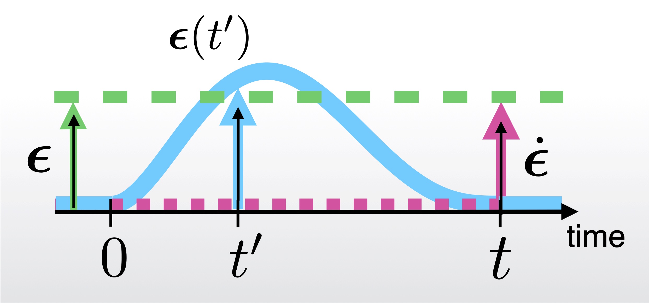
Figure 1: Illustration of the three types of dynamical transformations considered. The system is spatially displaced by ${\bm{\epsilon}}=\rm const$ at all times (green dashed), analogously to the operation in equilibrium. The system is dynamically displaced by ${\bm{\epsilon}}(t^{\prime})$, such that the spatial displacement vanishes at the boundaries of the considered time interval, ${\bm{\epsilon}}(0)={\bm{\epsilon}}(t)=0$ (cyan solid). The system is displaced instantaneously only at the latest time $t$, such that the differential displacement is $\dot{\bm{\epsilon}}dt$ (purple dotted).

Results and Discussion

Adiabatic state

We start with an initial illustration of Noether’s concept as applied to the grand potential $\Omega$. We consider spatial translations of the position coordinate r at fixed chemical potential $\mu$ and fixed temperature $T$. The system is under the influence of a one-body external potential $V_{\rm ext}({\bf r})$, cf. Fig. 2(a). We take $V_{\rm ext}({\bf r})$ to also describe container walls, such that there is no need for the system volume as a further thermodynamic variable. For the moment we only examine systems completely bounded by external walls. Systems with open boundaries are considered below. Clearly the value of the grand potential $\Omega$ is independent of the global location of a system. Hence spatial shifting by a (global) displacement vector ${\bm{\epsilon}}$ leaves the value of $\Omega$ invariant. To exploit this symmetry in a variational setting, note that the value of $\Omega$ depends on the function $V_{\rm ext}({\bf r})$, hence $V_{\rm ext}({\bf r})\to\Omega$ constitutes a functional map, at given $\mu$ and $T$. Here the grand potential is defined by its elementary Statistical Mechanics form $\Omega[V_{\rm ext}]=-k_{\text{B}}T\ln\Xi$, with the grand partition sum $\Xi$ depending functionally via the Boltzmann factor on $V_{\rm ext}({\bf r})$. The spatial displacement amounts to the operation $V_{\rm ext}({\bf r})\to V_{\rm ext}({\bf r}+{\bm{\epsilon}})$, cf. Fig. 2(b). For small ${\bm{\epsilon}}$ we can Taylor expand to linear order: $V_{\rm ext}({\bf r}+{\bm{\epsilon}})=V_{\rm ext}({\bf r})+\delta V_{\rm ext}({\bf r})$, where $\delta V_{\rm ext}({\bf r})={\bm{\epsilon}}\cdot\nabla V_{\rm ext}({\bf r})$ indicates the local change of the external potential that is induced by the shift. As $\Omega[V_{\rm ext}]$ is invariant under the shift (which can be shown by translating all particle coordinates in $\Xi$ accordingly), we have

$$\Omega[V_{\rm ext}] =\Omega[V_{\rm ext}+\delta V_{\rm ext}]$$

$$=\Omega[V_{\rm ext}]+\int d{\bf r}\frac{\delta\Omega[V_{\rm ext}]}{\delta V_{\rm ext}({\bf r})}{\bm{\epsilon}}\cdot\nabla V_{\rm ext}({\bf r}).$$ (1)

Here the second equality constitutes a functional Taylor expansion in $\delta V_{\rm ext}({\bf r})$ to linear order, and $\delta\Omega[V_{\rm ext}]/\delta V_{\rm ext}({\bf r})$ indicates the functional derivative of $\Omega[V_{\rm ext}]$ with respect to its argument, evaluated here at the unshifted function $V_{\rm ext}({\bf r})$, i.e. ${\bm{\epsilon}}=0$. It is a straightforward elementary exercise evans1979 ; hansen2013 to show via explicit calculation that $\delta\Omega[V_{\rm ext}]/\delta V_{\rm ext}({\bf r})=\rho({\bf r})$, where $\rho({\bf r})=\langle\sum_{i}\delta({\bf r}-{\bf r}_{i})\rangle_{\rm eq}$ is the microscopically resolved one-body density profile. Here ${\bf r}_{i}$ indicates the position of particle $i=1\ldots N$, with $N$ being the total number of particles, $\delta(\cdot)$ indicates the Dirac distribution, and the average is over the equilibrium distribution at fixed $\mu$ and $T$; the sum runs over all particles $i=1\ldots N$.

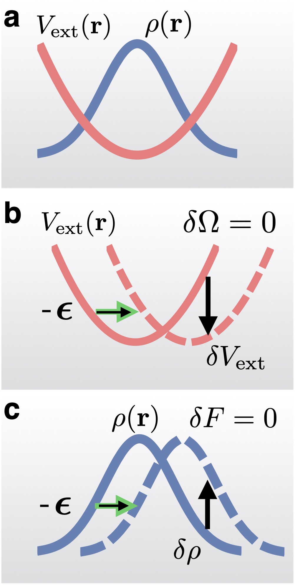
Figure 2: Illustrations of the effects induced by shifting in equilibrium. a In the presence of external potential $V_{\rm ext}({\bf r})$, the system develops an inhomogeneous density profile $\rho({\bf r})$, where r denotes the position coordinate. b Shifting the external potential by a displacement vector $-{\bm{\epsilon}}$ (green arrow) induces a local change in external potential $\delta V_{\rm ext}({\bf r})$ (black arrow) between the original (solid line) and the shifted external potential (dashed line); the grand potential is invariant, $\delta\Omega=0$. c The displaced density profile (dashed line) implies a local change $\delta\rho({\bf r})$ (black arrow) in comparison to the initial density profile (solid line), which leaves the intrinsic free energy unchanged, $\delta F=0$.

Comparing the left and right hand sides of (1) and noticing that ${\bm{\epsilon}}$ is arbitrary, we conclude

$${\bf F}_{\rm ext}^{\rm tot} =-\int d{\bf r}\rho({\bf r})\nabla V_{\rm ext}({\bf r})=0,$$ (2)

where we have defined the total external force ${\bf F}_{\rm ext}^{\rm tot}$ using the one-body fields $\rho({\bf r})$ and $V_{\rm ext}({\bf r})$. It is straightforward to show the equivalence with the more elementary form ${\bf F}_{\rm ext}^{\rm tot}=-\langle\sum_{i}\nabla_{i}V_{\rm ext}({\bf r}_{i})\rangle_{\rm eq}$, where $\nabla_{i}$ indicates the derivative with respect to ${\bf r}_{i}$. Clearly, (2) expresses the vanishing of the total external force. (Consider e.g. the gravitational weight of an equilibrium colloidal sediment being balanced by the force that the lower container wall exerts on the particles.)

Equation (2) was previously obtained by Baus baus1984 . Here we have identified it as a Noether sum rule for the case of spatial displacement of $\Omega[V_{\rm ext}]$. We can generate local sum rules by observing that (2) holds for any form of $V_{\rm ext}({\bf r})$ and that hence $V_{\rm ext}({\bf r})\to\rho({\bf r})$ constitutes a functional map (defined by the grand canonical average $\langle\hat{\rho}({\bf r})\rangle_{\rm eq}$, which features $V_{\rm ext}({\bf r})$ in the equilibrium many-body probability distribution). We hence functionally differentiate (2) by $V_{\rm ext}({\bf r}^{\prime})$, where ${\bf r}^{\prime}$ is a new position variable. The first and the $n$th functional derivatives yield, respectively, the identities

$$\nabla\rho({\bf r}) =-\int d{\bf r}^{\prime}\beta H_{2}({\bf r},{\bf r}^{\prime})\nabla^{\prime}V_{\rm ext}({\bf r}^{\prime}),$$ (3)

$$\sum_{\alpha=1}^{n}\nabla_{\alpha}H_{n} =-\int d{\bf r}_{n+1}\beta V_{\rm ext}({\bf r}_{n+1})\nabla_{n+1}H_{n+1},$$ (4)

where $\beta=1/(k_{\text{B}}T)$, with $k_{\text{B}}$ indicating the Boltzmann constant, $H_{2}({\bf r},{\bf r}^{\prime})=-\delta\rho({\bf r})/\delta\beta V_{\rm ext}({\bf r}^{\prime})$ is the two-body correlation function of density fluctuations, and $H_{n}=\delta H_{n-1}/\delta\beta V_{\rm ext}({\bf r}_{n})$ is its $n$-body version evans1979 ; hansen2013 . Here position arguments have been omitted for clarity: $H_{n}\equiv H_{n}({\bf r}_{1}\ldots{\bf r}_{n})$, and $\nabla_{\alpha}$ indicates the derivative with respect to ${\bf r}_{\alpha}$. The variable names ${\bf r}$ and ${\bf r}^{\prime}$ have been interchanged in (3) and $\nabla^{\prime}$ indicates the derivative with respect to ${\bf r}^{\prime}$. The derivation of (3) and (4) requires spatial integration by parts. Recall that boundary terms vanish as we only consider systems with impenetrable bounding walls.

The sum rule (3) has been obtained by LMBW lovett1976 ; wertheim1976 and by Evans evans1979 on the basis of shifting considerations. The present formulation based on Noether’s more general perspective allows to reproduce (3) with great ease and to generalize to the hierarchy (4), as previously obtained by Baus baus1984 . Equation (3) has the interpretation of the density gradient $\nabla\rho({\bf r})$ being stabilized by the action of the external force field, $-\nabla V_{\rm ext}({\bf r})$. The effect is mediated by $\beta H_{2}({\bf r},{\bf r}^{\prime})$, where the correlation of the density fluctuations is due to the coupled nature of the interparticle interactions. Equation (4) is the multi-body generalization of this mechanism. Via multiplying (3) by $V_{\rm ext}({\bf r})$, integrating over ${\bf r}$, and using (2), and iteratively repeating this process for all orders, one obtains a multi-body analogue of the vanishing external force (2):

$$\int d{\bf r}_{1}V_{\rm ext}({\bf r}_{1})\ldots\int d{\bf r}_{n}V_{\rm ext}({\bf r}_{n})\nabla_{\alpha}H_{n}=0,$$ (5)

for $\alpha=1\ldots n$.

We turn to intrinsic contributions. As Noether’s Theorem poses no restriction on the type of physical functional, we consider the intrinsic Helmholtz free energy $F[\rho]$ as a functional of the density profile as its natural argument. Here a functional Legendre transform hansen2013 ; evans1979 yields $F[\rho]=\Omega[V_{\rm ext}]-\int d{\bf r}(V_{\rm ext}({\bf r})-\mu)\rho({\bf r})$. Crucially, $F[\rho]$ is independent of $V_{\rm ext}({\bf r})$, and its excess (over ideal gas) contribution $F_{\rm exc}[\rho]$ is specific to the form of the interparticle interaction potential $u({\bf r}^{N})$; here we use the shorthand ${\bf r}_{1}\ldots{\bf r}_{N}\equiv{\bf r}^{N}$. The full intrinsic free energy functional consists of a sum of ideal gas and excess contributions, i.e. $F[\rho]=k_{\text{B}}T\int d{\bf r}\rho({\bf r})[\ln(\rho({\bf r})\Lambda^{D})-1]+F_{\rm exc}[\rho]$, where $\Lambda$ is the (irrelevant) thermal de Broglie wavelength and $D$ is the dimensionality of space.

As $u({\bf r}^{N})$ is globally translationally invariant, $F_{\rm exc}[\rho]$ will not change its value when evaluated at a spatially displaced density, $\rho({\bf r}+{\bm{\epsilon}})=\rho({\bf r})+\delta\rho({\bf r})$, where $\delta\rho({\bf r})={\bm{\epsilon}}\cdot\nabla\rho({\bf r})$, cf. Fig. 2(c). Hence in analogy to (1), we obtain $F_{\rm exc}[\rho]=F_{\rm exc}[\rho+\delta\rho]=F_{\rm exc}[\rho]+\int d{\bf r}(\delta F_{\rm exc}[\rho]/\delta\rho({\bf r})){\bm{\epsilon}}\cdot\nabla\rho({\bf r})$. Again ${\bm{\epsilon}}$ is arbitrary. As boundary terms vanish in the considered systems, integration by parts yields

$${\bf F}_{\rm ad}^{\rm tot} =-\int d{\bf r}\rho({\bf r})\nabla\frac{\delta F_{\rm exc}[\rho]}{\delta\rho({\bf r})}=\int d{\bf r}\rho({\bf r}){\bf f}_{\rm ad}({\bf r})=0,$$ (6)

where the first equality expresses the total internal force ${\bf F}_{\rm ad}^{\rm tot}=-\langle\sum_{i}\nabla_{i}u({\bf r}^{N})\rangle_{\rm eq}$ in DFT language. Hence (6) expresses the fact that the total internal force vanishes in equilibrium; the more general time-dependent case is treated below. The functional derivatives of $F_{\rm exc}[\rho]$ constitute direct correlation functions ornstein1914 ; hansen2013 ; evans1979 , with the lowest order being the one-body direct correlation function $c_{1}({\bf r})=-\delta\beta F_{\rm exc}[\rho]/\delta\rho({\bf r})$. The equilibrium (“adiabatic”) force field is simply ${\bf f}_{\rm ad}({\bf r})=k_{\text{B}}T\nabla c_{1}({\bf r})$. This one-body force field arises from the interparticle forces that all other particles exert on the particle that resides at position ${\bf r}$.

From the global internal Noether sum rule (6), we can obtain local sum rules by observing that (6) holds for all $\rho({\bf r})$ and hence that its functional derivative with respect to $\rho({\bf r})$ vanishes identically, i.e.,

$$\nabla c_{1}({\bf r}) =\int d{\bf r}^{\prime}c_{2}({\bf r},{\bf r}^{\prime})\nabla^{\prime}\rho({\bf r}^{\prime}),$$ (7)

$$\sum_{\alpha=1}^{n}\nabla_{\alpha}c_{n} =-\int d{\bf r}_{n+1}\rho({\bf r}_{n+1})\nabla_{n+1}c_{n+1},$$ (8)

where $c_{2}({\bf r},{\bf r}^{\prime})$ is the (inhomogeneous) two-body direct correlation function of liquid state theory hansen2013 ; $c_{n}\equiv c_{n}({\bf r}_{1}\ldots{\bf r}_{n})$ is the $n$-body direct correlation function, defined recursively via $c_{n+1}=\delta c_{n}/\delta\rho({\bf r}_{n+1})$. As identified by LMBW lovett1976 ; wertheim1976 and Evans evans1979 , (7) expresses the conversion of the density gradient, via the two-body direct correlations, to the locally resolved intrinsic force field; recall that ${\bf f}_{\rm ad}({\bf r})=k_{\text{B}}T\nabla c_{1}({\bf r})$. Via the Noether formalism the corresponding hierarchy (8) is obtained straightforwardly from repeated functional differentiation kayser1980 ; baus1984 ; lovett1991 with respect to $\rho({\bf r})$. Note that similar to the structure of (4), only consecutive terms of order $n$ and $n+1$ are directly coupled in (8). A multi-body version of (6) is obtained by multiplying (7) with $\rho({\bf r})$, integrating over ${\bf r}$, exploiting (6), and iterating for all orders. The result is:

$$\int d{\bf r}_{1}\rho({\bf r}_{1})\ldots\int d{\bf r}_{n}\rho({\bf r}_{n})\nabla_{\alpha}c_{n}=0,$$ (9)

for $\alpha=1\ldots n$. In the case $\alpha=n=1$ we recover (6).

The global sum rule (6) of vanishing total internal force can be straightforwardly obtained by more elementary analysis. We exploit translation invariance in this non-functional setting: $u({\bf r}^{N})\equiv u({\bf r}_{1}+{\bm{\epsilon}}\ldots{\bf r}_{N}+{\bm{\epsilon}})$. Then the derivative with respect to ${\bm{\epsilon}}$ vanishes, $0=\partial u({\bf r}_{1}+{\bm{\epsilon}}\ldots{\bf r}_{N}+{\bm{\epsilon}})/\partial{\bm{\epsilon}}=\sum_{i}\nabla_{i}u({\bf r}^{N})$. The latter expression follows from the chain rule and constitutes the total internal force (up to a minus sign), which hence vanishes for each microstate ${\bf r}^{N}$. The connection to (the many-body version of) Newton’s third law actio equals reactio becomes apparent in the rewritten form $-\nabla_{\alpha}u({\bf r}^{N})=\sum_{i\neq\alpha}\nabla_{i}u({\bf r}^{N})$, for $\alpha=1\ldots N$. The thermal equilibrium average is then trivial and on average ${\bf F}_{\rm ad}^{\rm tot}=0$. This argument is very general and it remains true if the average is taken over a nonequilibrium many-body distribution function. The total internal force in such a general situation is

$${\bf F}_{\rm int}^{\rm tot}=-\Big{\langle}\sum_{i}\nabla_{i}u({\bf r}^{N})\Big{\rangle}=0,$$ (10)

where the average is taken over the nonequilibrium many-body probability distribution at time $t$. We have hence proven that the total internal force vanishes for all times $t$. In addition, the particles can possess additional degrees of freedom ${\bm{\omega}}_{i}$, $i=1\ldots N$, as is the case for the orientation vectors of active Brownian particles, to which we return after first laying out the setup in nonequilibrium.

Nonequilibrium states

To be specific, we consider overdamped Brownian motion, at constant temperature $T$ and with no hydrodynamic interactions present hansen2013 , as described by the Smoluchowski (Fokker-Planck) equation. The microscopically resolved local internal force field is ${\bf f}_{\rm int}({\bf r},t)=-\langle\sum_{i}\delta({\bf r}-{\bf r}_{i})\nabla_{i}u({\bf r}^{N})\rangle/\rho({\bf r},t)$, where the average is over the nonequilibrium distribution (which evolves in time according to the Smoluchowski equation) at time $t$. The total internal force is then the spatial integral ${\bf F}_{\rm int}^{\rm tot}=\int d{\bf r}\rho({\bf r},t){\bf f}_{\rm int}({\bf r},t)$. Applying Noether’s Theorem to the nonequilibrium case requires to have a variational description, as is provided by PFT schmidt2013pft . Here the variational fields are the time-dependent density profile $\rho({\bf r},t)$ and the time-dependence one-body current ${\bf J}({\bf r},t)=\langle\sum_{i}\delta({\bf r}-{\bf r}_{i}){\bf v}_{i}\rangle$, where ${\bf v}_{i}({\bf r}^{N},t)$ is the configurational velocity of particle $i$. The microscopically resolved average velocity profile is ${\bf v}({\bf r},t)={\bf J}({\bf r},t)/\rho({\bf r},t)$. PFT ascertains the splitting ${\bf f}_{\rm int}({\bf r},t)={\bf f}_{\rm ad}({\bf r},t)+{\bf f}_{\rm sup}({\bf r},t)$, where the adiabatic force field is that in a corresponding equilibrium (“adiabatic”) system with identical instantaneous density profile, ${\bf f}_{\rm ad}({\bf r},t)=-\nabla\delta F_{\rm exc}[\rho]/\delta\rho({\bf r},t)$ and ${\bf f}_{\rm sup}({\bf r},t)$ is the superadiabatic internal force field, obtained as ${\bf f}_{\rm sup}({\bf r},t)=-\delta P_{t}^{\rm exc}[\rho,{\bf J}]/\delta{\bf J}({\bf r},t)$, where $P_{t}^{\rm exc}[\rho,{\bf J}]$ is the superadiabatic excess free power functional schmidt2013pft .

Crucially, ${\bf f}_{\rm ad}({\bf r},t)$ is a density functional, independent of the flow in the system, while ${\bf f}_{\rm sup}({\bf r},t)$ is a kinematic functional, i.e. with dependence on both $\rho({\bf r},t)$ and ${\bf J}({\bf r},t)$, including memory, i.e. dependence on the value of the fields at times $<t$. As the local force fields split into adiabatic and superadiabatic contributions, so do the total forces: ${\bf F}_{\rm int}^{\rm tot}=\int d{\bf r}\rho{\bf f}_{\rm int}=\int d{\bf r}\rho{\bf f}_{\rm ad}+\int d{\bf r}\rho{\bf f}_{\rm sup}\equiv{\bf F}_{\rm ad}^{\rm tot}+{\bf F}_{\rm sup}^{\rm tot}$. We have seen above that ${\bf F}_{\rm int}^{\rm tot}={\bf F}_{\rm ad}^{\rm tot}=0$. Hence also

$${\bf F}_{\rm sup}^{\rm tot} =-\int d{\bf r}\rho({\bf r},t)\frac{\delta P_{t}^{\rm exc}[\rho,{\bf J}]}{\delta{\bf J}({\bf r},t)}\equiv\int d{\bf r}\rho{\bf f}_{\rm sup}=0.$$ (11)

While the above reasoning required to rely on the many-body level, the same result (11) can be straightforwardly obtained in a pure Noetherian way, by considering an instantaneous shift of coordinates at time $t$, i.e. ${\bf J}({\bf r},t)\to{\bf J}({\bf r},t)-\dot{\bm{\epsilon}}\rho({\bf r},t)$, cf. Fig. 3(a). (Fig. 3 gives an overview of the three different types of shifting.) Here $\dot{\bm{\epsilon}}$ is the corresponding instantaneous change in velocity with ${\bf v}({\bf r},t)\to{\bf v}({\bf r},t)-\dot{\bm{\epsilon}}$, as obtained by dividing the current by the density profile. Due to the overdamped nature of the Smoluchowski dynamics, the internal interactions are unaffected and the shift constitutes a symmetry operation for the generator of the superadiabatic forces, $P_{t}^{\rm exc}[\rho,{\bf J}]$. Hence the instantaneous current perturbation $\delta{\bf J}({\bf r},t)=-\dot{\bm{\epsilon}}\rho({\bf r},t)$ that is generated by the invariance transformation leads to $P_{t}^{\rm exc}[\rho,{\bf J}]=P_{t}^{\rm exc}[\rho,{\bf J}+\delta{\bf J}]=P_{t}^{\rm exc}[\rho,{\bf J}]-\int d{\bf r}(\delta P_{t}^{\rm exc}[\rho,{\bf J}]/\delta{\bf J}({\bf r},t))\cdot\dot{\bm{\epsilon}}\rho({\bf r},t)$. As $\dot{\bm{\epsilon}}$ is arbitrary, we obtain (11). Treating the dynamical adiabatic contribution $\dot{F}[\rho]=\int d{\bf r}{\bf J}({\bf r},t)\cdot\nabla\delta F_{\rm exc}[\rho]/\delta\rho({\bf r},t)$ in the same way, we re-obtain (6). As Noether’s theorem is converse, it allows for alternative reasoning: the invariance of $P_{t}^{\rm exc}[\rho,{\bf J}]$ to the instantaneous shift of the current (or analogously of the velocity) can hence be derived from (11) by simply reversing the above chain of arguments.

We can generate nonequilibrium sum rules by differentiating the Noether identity (11) with respect to ${\bf J}({\bf r},t)$, which yields

$$\int d{\bf r}^{\prime}{\sf M}_{2}({\bf r},{\bf r}^{\prime},t)\rho({\bf r}^{\prime},t) =0,$$ (12)

where ${\sf M}_{2}({\bf r},{\bf r}^{\prime},t)=-\beta\delta^{2}P_{t}^{\rm exc}[\rho,{\bf J}]/\delta{\bf J}({\bf r},t)\delta{\bf J}({\bf r}^{\prime},t)$ is the tensorial two-body equal-time direct correlation function brader2013noz ; brader2014noz . Its $n$-body version is obtained from ${\sf M}_{n+1}({\bf r}_{1}\ldots{\bf r}_{n+1},t)=\delta{\sf M}_{n}({\bf r}_{1}\ldots{\bf r}_{n},t)/\delta{\bf J}({\bf r}_{n+1},t)$, and it satisfies the hierarchy

$$\int d{\bf r}_{n+1}{\sf M}_{n+1}\rho({\bf r}_{n+1},t)=0,$$ (13)

as obtained by differentiating (12) repeatedly with respect to the current.

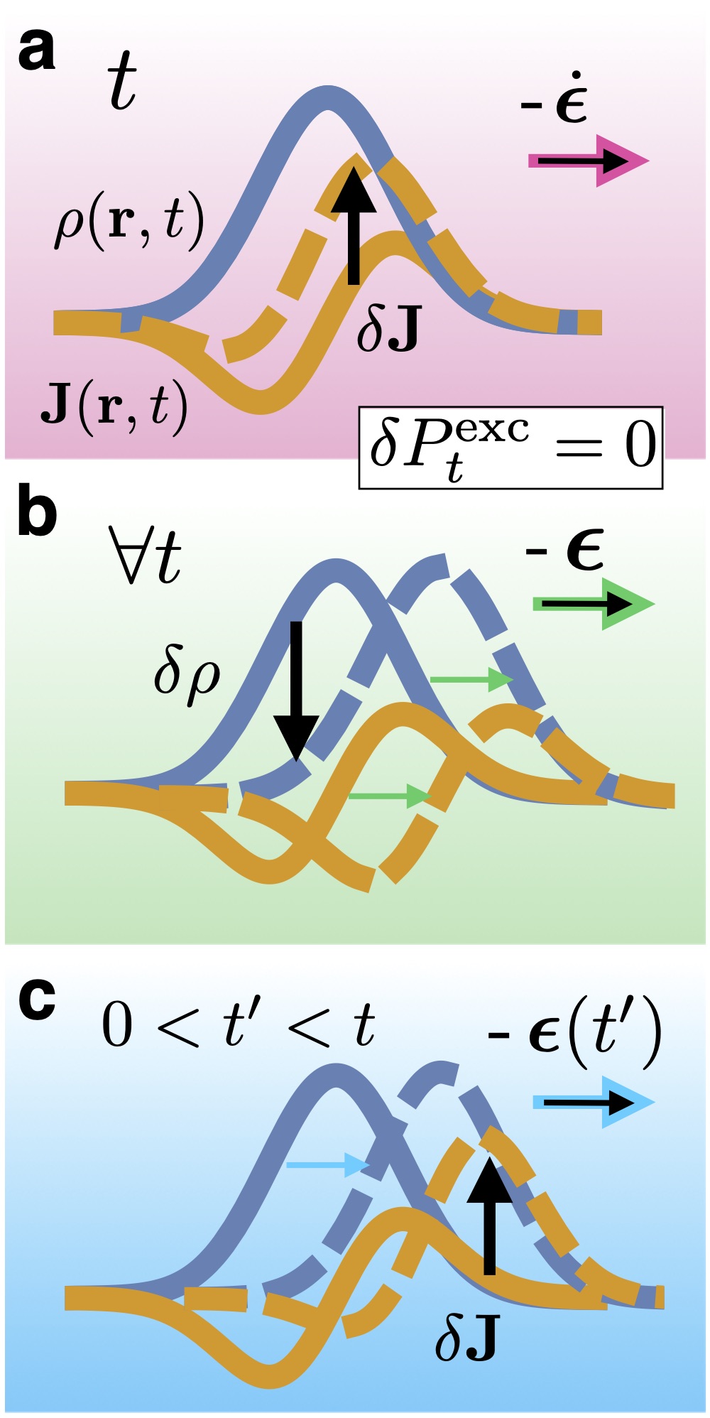
Figure 3: Illustrations of the effects induced by shifting in nonequilibrium. All transformations affect both the density profile $\rho({\bf r},t)$ (blue) and the current profile ${\bf J}({\bf r},t)$ (yellow), while the superadiabatic excess power functional is invariant, $\delta P_{t}^{\rm exc}=0$. Here $t$ indicates the time and r is the position coordinate. a An instantaneous spatial shift by $\dot{\bm{\epsilon}}$ at time $t$ induces a current change $\delta{\bf J}=-\dot{\bm{\epsilon}}\rho$. b A static shift by ${\bm{\epsilon}}=\rm const$ is applied at all times $t$. c A time-dependent shift ${\bm{\epsilon}}(t^{\prime})$ is applied between inital time 0 and final time $t$ of the considered time interval.

Open boundaries

All our considerations have been based on applying the symmetry operation to the entire system confined by external walls. The effects of these system walls are modelled by a suitable form of $V_{\text{ext}}({\bf r})$. The position integrals formally run over all space, with the cutoff provided by hard (or steeply rising) external wall potentials. In many practical and relevant situations, it is more useful to consider a system with open boundaries. Alternatively one can consider only a subvolume $V$ of the entire system, and restrict the accounting of force contributions to those particles that reside inside of $V$ at a given time. In doing so, one needs to take account of boundary effects requardt1988 , as the boundaries of $V$ are open, such that interparticle forces can be transmitted, and flow can occur.

In case that there are no net boundary contributions, all previous derived sum rules still hold. This includes e.g. an effectively one-dimensional system in planar geometry that evolves to the same bulk state at the left and right boundaries or if the boundary conditions are periodic. In both cases left and right boundary terms are equal up to a minus sign and hence cancel each other. This example can be generalized straightforwardly to more complex geometries.

For non-vanishing net boundary terms additional contributions arise in the above sum rules. These contributions occur if the system develops different (bulk) states, e.g. for $x\to\pm\infty$ as is relevant for bulk phase separation (see the section below). We demonstrate that such cases can be systematically treated in the current framework, by exemplary considering the total internal force. Then boundary force contributions arise due to an imbalance of “outside” particles that exert forces on “inside” particles. The outside particles are per definition excluded from the accounting of the total internal force exerted by all particles inside of $V$. The sum of all interactions between inside particles vanishes due to the global internal Noether sum rule (10). For simplicity we restrict ourselves to systems that interact via short-ranged pairwise central forces, where $\textbf{F}_{ij}$ indicates the force on particle $i$ exerted by particle $j$. So only forces exerted from an inside to an outside particle contribute. The total internal force that acts on $V$ is hence $\textbf{F}_{\text{int}}^{\text{tot}}=\langle\sum_{ij}^{\prime}\textbf{F}_{ij}\rangle$, where the restricted sum (prime) runs only over those $i\in V$ and $j\in\bar{V}$, where $\bar{V}$ indicates the complement of $V$. The total internal force between particles inside of $V$, i.e. $i\in V$ and $j\in V$, vanishes due to (10). We then rewrite $\textbf{F}_{\text{int}}^{\text{tot}}$ via inserting the identity $\int d{\bf r}\delta({\bf r})=1$ twice into the average. Then the restrictions of the sums can be transferred to restrictions on the spatial integration domains. As a result the total internal force acting on $V$ can be expressed via correlation functions as

$${\bf F}_{\text{int}}^{\text{tot}} =\int_{V}d{\bf r}\int_{\bar{V}}d{\bf r}^{\prime}\Big{\langle}\sum_{i,j\neq i}\delta({\bf r}-{\bf r}_{i})\delta({\bf r}^{\prime}-{\bf r}_{j})\textbf{F}_{ij}\Big{\rangle}$$ (14)

$$=-\int_{V}d{\bf r}\int_{\bar{V}}d{\bf r}^{\prime}\rho({\bf r})\rho({\bf r}^{\prime})g({\bf r},{\bf r}^{\prime})\nabla\phi(|{\bf r}-{\bf r}^{\prime}|),$$ (15)

where $\phi(r)$ indicates the interparticle pair potential as a function of interparticle distance $r$. In order to obtain the form (15) we have identified the many-body definition of the radial distribution function $g({\bf r},{\bf r}^{\prime})=\big{\langle}\sum_{i,j\neq i}\delta({\bf r}-{\bf r}_{i})\delta({\bf r}^{\prime}-{\bf r}_{j})\big{\rangle}/(\rho({\bf r})\rho({\bf r}^{\prime}))$. Recall that the pair distribution function $g$ and the density-density correlation function $H_{2}$, as used in (3)-(5), are related via $H_{2}({\bf r},{\bf r}^{\prime})=(g({\bf r},{\bf r}^{\prime})-1)\rho({\bf r})\rho({\bf r}^{\prime})+\delta({\bf r}-{\bf r}^{\prime})\rho({\bf r})$. Equation (15) still holds for non-conservative interparticle forces, when $-\nabla\phi(|{\bf r}-{\bf r}^{\prime}|)$ is replaced by the (nongradient) interparticle force field. We demonstrate in the following section the practical relevance of these considerations.

Phase coexistence

We turn to situations of phase coexistence. As we demonstrate, considering a large, but finite subvolume $V$ of the entire system is useful but it also requires to take boundary terms into account. Here we take $V$ to be cuboidal and to contain the free (planar) interface between two coexisting phases, see Fig. 4(a) for a graphical illustration. The volume boundaries parallel to the interface are taken to be seated deep inside either bulk phase. The internal force contributions on those faces of $V$ that “cut through” the interface, i.e. have a normal that is perpendicular to the interface normal, vanish by symmetry. It remains to evaluate (15) over each of the two faces in the respective bulk region. Therefore the position dependences simplify to $\rho(\textbf{r})=\rho_{b}=\text{const}$, where $\rho_{b}$ indicates the bulk number density, and the inhomogeneous pair distribution function simplifies as $g(\textbf{r},\textbf{r}^{\prime})=g(|\textbf{r}-\textbf{r}^{\prime}|)$. Furthermore only force contributions collinear with ${\bf e}$, the outer interface normal of the considered bulk phase $b$, contribute. For a single face in bulk phase $b$, it is straightforward to show that the result is the virial pressure multiplied by the interface area $A$, i.e. the force $Ap^{b}_{\text{int}}\textbf{e}$, where the internal interaction pressure $p^{b}_{\text{int}}$ in phase $b$ is e.g. given via the Clausius virial hansen2013 , $p^{b}_{\text{int}}=-\frac{\pi}{2}\rho^{2}_{b}\int\limits_{0}^{r_{0}}dr\,r^{2}g(r)\frac{d\phi}{dr}$ in two spatial dimensions. (The argument remains general.) The constant $r_{0}$ denotes the range of the interparticle interactions.

The total force density balance for equilibrium phase separation contains thermal diffusion and the internal force density, which cancel each other,

$$0=-k_{\text{B}}T\nabla\rho(\textbf{r})+\rho(\textbf{r})\textbf{f}_{\text{int}}(\textbf{r}).$$ (16)

Integration over the volume $V$ yields the total force which is proportional to the pressure. Hence the total internal force $\textbf{F}^{\text{tot}}_{\text{int}}=\int_{V}d\textbf{r}\,\rho\textbf{f}_{\text{int}}$ on $V$, cf. (15), amounts to the pressure difference $(p_{\rm int}^{g}-p_{\rm int}^{l})A{\bf e}$, where ${\bf e}$ is the (unit vector) normal of the interface, pointing from, say, the gas (index $g$) to the liquid phase (index $l$). The total diffusive force is $(p_{\rm id}^{g}-p_{\rm id}^{l})A{\bf e}$ with the pressure of the ideal gas $p_{\rm id}=k_{\text{B}}T\rho$, evaluated at the gas ($\rho_{g}$) and liquid bulk density ($\rho_{l}$). As there are no external forces ($V_{\rm ext}\equiv 0$) then requesting the volume $V$ to be forcefree amounts to $p_{\rm tot}^{g}=p_{\rm tot}^{l}$, where the total pressure is the sum $p_{\rm tot}=p_{\rm id}+p_{\rm int}$. Hence the boundary consideration yields the mechanical equilibrium condition of equality of pressure in the coexisting phases.

We conclude that the internal interactions that occur across the free interface do not influence the (bulk) balance of the pressure at phase coexistence, as the net effect of these interactions vanishes. At the heart of this argument lies Noether’s theorem for invariance against spatial displacements.

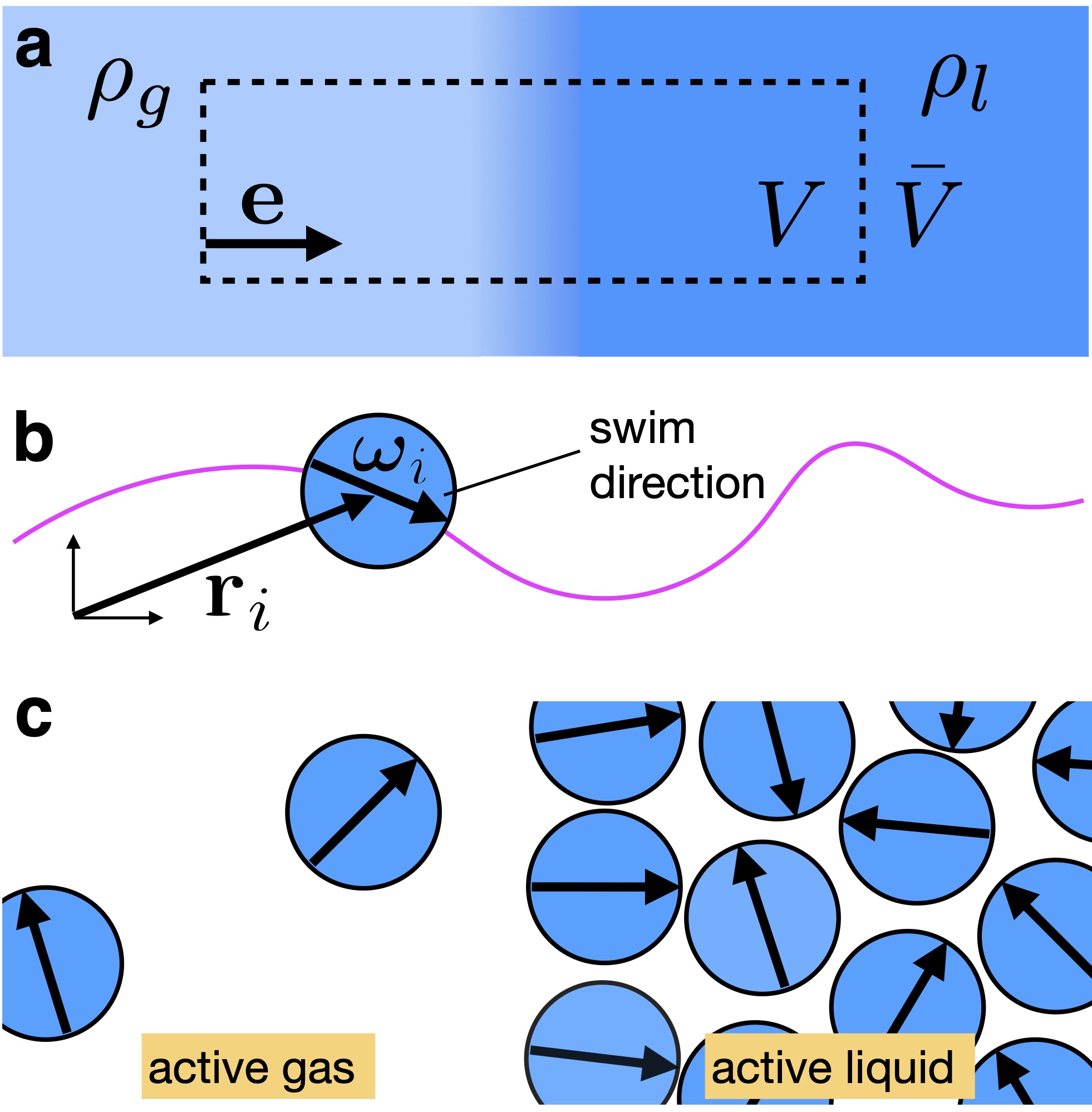
Figure 4: Phase separation into macroscopically distinct phases. a Illustration of the geometry of phase separation of passive or active particles. Shown are the gaseous $\rho_{g}$ and liquid $\rho_{l}$ plateau values of the density profile (indicated by the colour gradient) and the direction vector $\bf e$ normal to the interface. The total system volume $V+\bar{V}$ consists of the subvolume $V$ and its complement $\bar{V}$. b Illustration of an active Brownian particle (blue disc) with position $\textbf{r}_{i}$ and orientation $\bm{\omega}_{i}$ undergoing translational and rotational diffusion. The self propulsion along $\bm{\omega}_{i}$ creates directed motion as indicated by the trajectory (magenta line). c Schematics of motility-induced phase separation into active gas (left) and active liquid phases (right). The arrows indicate the orientations $\bm{\omega}_{i}$ of the active particles. The interface is polarized.

Anisotropic particles

We turn to anisotropic interparticle interactions, where ${\bm{\omega}}_{i}$, $\bm{\varpi}_{i}$ are two perpendicular unit vectors that describes the particle orientation in space. Such systems are described by an interparticle interaction potential $u({\bf r}^{N},{\bm{\omega}}^{N},\bm{\varpi}^{N})$, which is assumed a priori to be invariant under spatial translations. Similarly one-body fields in general depend on position ${\bf r}$ and orientations ${\bm{\omega}}$ and $\bm{\varpi}$ of the particles, e.g. $V_{\text{ext}}({\bf r},{\bm{\omega}},\bm{\varpi})$ for the external field. The fully resolved one-body density distribution is $\rho({\bf r},{\bm{\omega}},\bm{\varpi},t)=\langle\sum_{i}\delta({\bf r}-{\bf r}_{i})\delta({\bm{\omega}}-{\bm{\omega}}_{i})\delta(\bm{\varpi}-\bm{\varpi}_{i})\rangle$.

It is straightforward to ascertain that all the above (force) sum rules for translation remain valid, as the orientations are unaffected by translations, upon trivially generalizing from position-only to position-orientation integration, $\int d{\bf r}\to\int d{\bf r}d{\bm{\omega}}d\bm{\varpi}$ etc.

In the following for simplicity of notation we first consider uniaxial particles. Uniaxial particles depend only on one single orientation ${\bm{\omega}}_{i}$, as the particles are rotationally invariant around this vector. Hence the $\bm{\varpi}$-dependence of both the one- and many-body quantities vanish and the total integral simplifies to $\int d{\bf r}d{\bm{\omega}}$.

Motility induced phase separation

We use active Brownian particles as an example for uniaxial particles. For simplicity we consider spherical particles (discs) in two dimensions. The particles repel each other and they undergo self-propelled motion along their orientation vector ${\bm{\omega}}$. Hence an additional one-body force $\gamma s{\bm{\omega}}$ acts on each swimmer, with $\gamma$ the friction constant and $s$ the speed of free swimming. This self-propulsion creates characteristic trajectories (see Fig. 4(b) for a schematic) which are also affected by thermal diffusion (omitted in the schematic) of the particle position $\textbf{r}_{i}$ and orientation ${\bm{\omega}}_{i}$. Experimental realizations of active Brownian particles include e.g. Janus colloids driven by photon nudging nudge1 ; nudge2 ; nudge3 ; nudge4 ; nudge5 . If the density is high enough, motility induced phase separation (MIPS) into an active gas and active liquid phase occurs for high enough values of the swim speed $s$, cf. Fig. 4(c).

The force density balance (see e.g. the work of Hermann et al. hermann2019pre ) of such a system in steady state (no time dependence) is

$$\gamma\textbf{J}(\textbf{r},{\bm{\omega}})= -k_{\text{B}}T\nabla\rho(\textbf{r},{\bm{\omega}})+\rho(\textbf{r},{\bm{\omega}})\textbf{f}_{\text{int}}(\textbf{r},{\bm{\omega}})$$

$$+\gamma s\rho(\textbf{r},{\bm{\omega}}){\bm{\omega}}+\rho(\textbf{r},{\bm{\omega}})\textbf{f}_{\text{ext}}(\textbf{r},{\bm{\omega}}).$$ (17)

The (negative) frictional force density on the left hand side is balanced with the ideal gas contribution (first term), the interparticle interactions (second term), the self-propulsion (third term) and the external contribution (fourth term) on the right hand side. As in case of the equilibrium phase separation we integrate (17) over the volume $V$ (see Fig. 4(a) for an illustration) and over all orientations ${\bm{\omega}}$. In the following we discuss each term separately. For simplicity we assume planar geometry of the system and we assume a vanishing external force, $\textbf{f}_{\text{ext}}(\textbf{r},{\bm{\omega}})=0$. Here, the interaction contribution $p_{\rm int}A{\bf e}$ is obtained as above in equilibrium via (15), but the virial is averaged over the nonequilibrium steady state many-body probability distribution. The integral over the current $\int d\textbf{r}d{\bm{\omega}}\textbf{J}$ is assumed to vanish in steady state.

The total swim force that acts on $V$ contributes to the total force. In the considered situation, the swim force is entirely due to the polarization $\textbf{M}_{\text{tot}}=\int d\textbf{r}d{\bm{\omega}}\,{\bm{\omega}}\rho$ of the free interface in MIPS. Particles at the interface tend to align against the dense phase paliwal2018 if they interact purely repulsively (cf. Fig. 4(c)), and they align against the dilute phase if interparticle attraction is present paliwal2017activeLJ . No such spontaneous polarization occurs in bulk. The interface polarization is a state function of the coexisting phases hermann2020polarization as verified both experimentally leipzig1 and numerically leipzig2 . The total swim force that acts on $V$ is $(p_{\rm swim}^{g}-p_{\rm swim}^{l})A{\bf e}$, where $p_{\rm swim}^{b}=\gamma sJ_{b}/(2D_{\rm rot})$, with $J_{b}$ the bulk current in the forward direction ${\bm{\omega}}$ and $D_{\rm rot}$ indicating the rotational diffusion constant. Apart from the ideal term no further forces act, cf. the force density balance (17). The integral over the ideal term is similar to the total equilibrium ideal contribution, $(p^{g}_{\text{id}}-p^{l}_{\text{id}})A{\bf e}$. Combination of all results from integration yields the total force balance.

As the negative integral over the force density defines the nonequilibrium pressure, the volume $V$ being force free amounts to $p_{\rm tot}^{g}=p_{\rm tot}^{l}$, where $p_{\rm tot}=p_{\rm id}+p_{\rm int}+p_{\rm swim}$. Hermann et al. hermann2019pre demonstrates the splitting of $p_{\rm int}$ into adiabatic and superadiabatic contributions and presents results for the phase diagram based on approximate forms for the interparticle interaction contributions. The pressure, especially its swim contribution is defined in various different ways in the literature pressure1 ; pressure2 ; pressure3 ; pressure4 ; pressure5 ; pressure6 .

We conclude that the internal interactions that occur across the free interface do not influence the (bulk) balance of the pressure at phase coexistence, as the net effect of these interactions vanishes. In essence this argument follows from Noether’s theorem for invariance against spatial displacements.

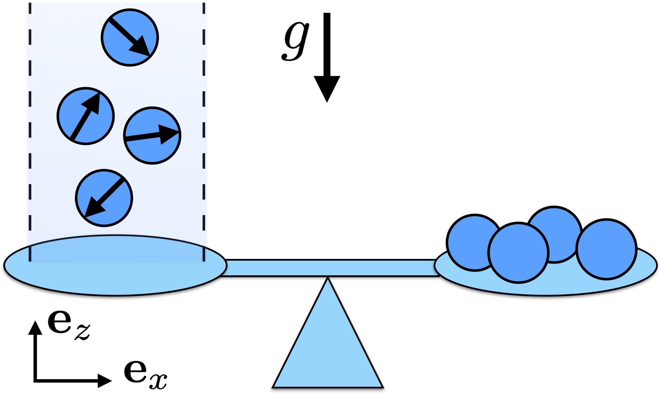
Figure 5: Illustration of sedimentation of active Brownian particles under gravity $g$. The active particles with orientation $\bm{\omega}$ (black arrows) are confined by a lower wall and periodic boundary conditions on the sides (dashed lines). The total force that the swimming particles exert on the bottom wall (left scale pan) is equal to their weight (right scale pan) in steady states of the system.

Active sedimentation

Sedimentation under the influence of gravity is a ubiquitous phenomenon in soft matter that has attracted considerable interest, e.g. for colloidal mixtures dani1 ; dani2 ; dani3 ; dani4 and for active systems sedi1 ; sedi2 ; sedi3 ; sedi4 . As sedimentation is a force driven phenomenon the Noether sum rules apply directly, as we show in the following.

We assume that the system is translationally invariant in the $x$-direction and that an impenetrable wall at $z=0$ acts as a lower boundary of the system lee2013 (cf. Fig. 5). We assume the wall-particle interaction potential to be short-ranged. Its precise form is irrelevant for the following considerations. The force density balance for such a system is (17) with the external force field chosen as

$$\textbf{f}_{\text{ext}}(\textbf{r},{\bm{\omega}})=-mg\textbf{e}_{z}+\textbf{f}_{\text{wall}}(\textbf{r},{\bm{\omega}}),$$ (18)

where $m$ denotes the mass of a particle, $g$ is the gravitational acceleration and $\textbf{e}_{z}$ indicates the unit vector in $z$-direction. Hence the external force field $\textbf{f}_{\text{ext}}$ consists of gravity and the wall contribution $\textbf{f}_{\text{wall}}$.

To proceed we integrate the force density balance over all positions r in the volume $V$ and over all orientations ${\bm{\omega}}$. The total integral of the density distribution (per radiant) $\int d\textbf{r}d{\bm{\omega}}\rho$, as appears in the gravitational term, gives the total number of particles $N$. The integral over the total current $\int d\textbf{r}d{\bm{\omega}}\,\textbf{J}$ is proportional to the center of mass velocity $\textbf{v}_{\text{cm}}(t)=\int d\textbf{r}d{\bm{\omega}}\,\rho\textbf{v}/\int d\textbf{r}d{\bm{\omega}}\,\rho=\frac{1}{N}\int d\textbf{r}d{\bm{\omega}}\,\textbf{J}$. Here $\textbf{v}_{\text{cm}}(t)$ is a global quantity and hence it is independent of both position and orientation. We first only consider steady states, so the center of mass velocity $\textbf{v}_{\text{cm}}(t)=0$ and hence the total current vanishes. The total thermal diffusion term vanishes because $\int_{V}d\textbf{r}\,\nabla\rho=\int_{\delta V}d\textbf{S}\,\rho=0$ as there is no contribution of $\rho$ from the boundaries $\partial V$ of the integration volume $V$. At the upper and lower boundary the density is zero as it vanishes in the wall and also for $z\to\infty$. The left and the right boundary contributions cancel each other as the density is independent of $x$ due to translational invariance. The total internal interaction force density vanishes, $\textbf{F}_{\text{int}}^{\text{tot}}=\int d\textbf{r}d{\bm{\omega}}\,\rho\textbf{f}_{\text{int}}=0$, using the global internal Noether sum rule (10). The integrated swim force density is proportional to the total polarization $\textbf{M}_{\text{tot}}=\int d\textbf{r}d{\bm{\omega}}\,{\bm{\omega}}\rho$. This quantity vanishes, $\textbf{M}_{\text{tot}}=0$, as there is no net flux through the boundaries in steady state (see Eq. (10) by Hermann et al. hermann2020polarization ). Combination of all integrals yields the relation

$$\textbf{F}^{\text{tot}}_{\text{wall}}=\int d\textbf{r}d{\bm{\omega}}\,\rho\textbf{f}_{\text{wall}}=mgN\textbf{e}_{z}.$$ (19)

Hence the $z$-component of the total force on the wall $F^{\text{tot}}_{\text{wall}}$ is equal to the total gravitational force acting on all particles (see Fig. 5 for a graphical representation). Equation (19) of course also holds for passive colloids ($s=0$).

Keeping the translational invariance in the $x$-direction, we next turn to time dependent systems. Therefore all one-body field in (17) additionally depend on the time $t$. Integration of the force density balance (17) gives identical results for the thermal diffusion, the internal force density and for the gravitational contribution as in the above case of steady state. Even for the time-dependent dynamics these integrals are independent of time $t$. The total wall force density is given as $\textbf{F}_{\text{wall,tot}}=F^{\text{tot}}_{\text{wall}}\textbf{e}_{z}$ and it only acts along the unit vector in the $z$-direction $\textbf{e}_{z}$, due to the symmetry of the system. The integral of the self-propulsion term is still proportional to the total polarisation. However, the total polarization does not vanish in general but decays exponentially (see Eq. (21) by Hermann et al. hermann2020polarization ),

$$\textbf{M}_{\text{tot}}(t)=\textbf{M}_{\text{tot}}(0)e^{-D_{\text{rot}}t},$$ (20)

where $\textbf{M}_{\text{tot}}(0)$ indicates the initial polarization at time $t=0$ and the time constant $1/D_{\text{rot}}$ is the inverse rotational diffusion constant. Similarly, integration of the current still gives the (time-dependent) center of mass velocity $\textbf{v}_{\text{cm}}(t)$.

Insertion of these results into the spatial and orientational integration of (17) leads to the total friction force

$$\gamma N\textbf{v}_{\text{cm}}(t)=s\gamma\textbf{M}_{\text{tot}}(0)\,e^{-D_{\text{rot}}t}+F^{\text{tot}}_{\text{wall}}(t)\,\textbf{e}_{z}-mgN\textbf{e}_{z},$$ (21)

which is hence a direct consequence of the Noether sum rule (10). We find that the $x$-component of the center of mass velocity decays simultaneously with the total polarization, cf. the first term on the right hand side of (21). The $z$-component of $\textbf{v}_{\text{cm}}(t)$ depends on $\textbf{M}_{\text{tot}}(t)$ and additionally on the time-dependent total force exerted by the wall and the total graviational force. Hence measuring the total force on the wall (i.e. by weighing, cf. Fig. 5) and knowledge of the total initial polarization and the total particle number allows one to determine the center of mass velocity. Note that in the limit of long times, $t\to\infty$, the total polarization vanishes and this system evolves to a steady state. Hence the center of mass velocity vanishes and (19) is recovered. As we have demonstrated both statements (19) and (21) ultimately follow from the global Noether identity (10).

Rotational invariance

We return to the general case and initially consider spatial rotations in systems of spheres, i.e. systems where $u({\bf r}^{N})$ depends solely on (relative) particle positions, and where it is invariant under global rotation of all ${\bf r}^{N}$ around the origin. We parameterize the rotation by a vector ${\bf n}$. The direction of ${\bf n}$ indicates the rotation axis and the modulus $|{\bf n}|$ is the angle of rotation. To lowest nonvanishing order, the rotation amounts to ${\bf r}\to{\bf r}+{\bf n}\times{\bf r}$. One-body functions change accordingly: the external potential undergoes $V_{\rm ext}({\bf r})\to V_{\rm ext}({\bf r})+\delta V_{\rm ext}({\bf r})$, with $\delta V_{\rm ext}({\bf r})=({\bf n}\times{\bf r})\cdot\nabla V_{\rm ext}({\bf r})$ and the density profile $\rho({\bf r})\to\rho({\bf r})+\delta\rho({\bf r})$ with $\delta\rho({\bf r})=({\bf n}\times{\bf r})\cdot\nabla\rho({\bf r})$. Much of the reasoning of the above case of spatial displacement can be applied readily: $\Omega[V_{\rm ext}]$ is invariant under the rotation, and $\delta\Omega=\int d{\bf r}(\delta\Omega/\delta V_{\rm ext}({\bf r}))\delta V_{\rm ext}({\bf r})=\int d{\bf r}\rho({\bf r})({\bf n}\times{\bf r})\cdot\nabla V_{\rm ext}({\bf r})=0$. As the rotation vector ${\bf n}$ is arbitrary, we can conclude that the total external torque ${\bm{\mathcal{T}}}_{\rm ext}^{\rm tot}$ vanishes in equilibrium baus1984 ,

$${\bm{\mathcal{T}}}_{\rm ext}^{\rm tot}\equiv-\int d{\bf r}\rho({\bf r})({\bf r}\times\nabla V_{\rm ext}({\bf r}))=0.$$ (22)

As this holds true for any form of the applied $V_{\rm ext}({\bf r})$, we can differentiate with respect to $V_{\rm ext}({\bf r}^{\prime})$, and obtain baus1984

$${\bf r}\times\nabla\rho({\bf r})=-\int d{\bf r}^{\prime}\beta H_{2}({\bf r},{\bf r}^{\prime})({\bf r}^{\prime}\times\nabla^{\prime}V_{\rm ext}({\bf r}^{\prime})),$$ (23)

$$\sum_{\alpha=1}^{n}({\bf r}_{\alpha}\times\nabla_{\alpha}H_{n})=$$

$$\quad-\int d{\bf r}_{n+1}\beta V_{\rm ext}({\bf r}_{n+1})({\bf r}_{n+1}\times\nabla_{n+1}H_{n+1}).$$ (24)

The excess free energy density functional $F_{\rm exc}[\rho]$ can be treated accordingly. It is invariant under rotation, as its sole dependence is on $u({\bf r}^{N})$, which by assumption is rotationally invariant. Analogous to this reasoning, we obtain the result that the total interparticle adiabatic torque ${\bm{\mathcal{T}}}_{\rm ad}^{\rm tot}$ vanishes,

$${\bm{\mathcal{T}}}_{\rm ad}^{\rm tot}=\int d{\bf r}\rho({\bf r})({\bf r}\times{\bf f}_{\rm ad}({\bf r}))=0.$$ (25)

Differentiation with respect to the independent field $\rho({\bf r})$ once and $n$ times yields the respective identities baus1984 ; lovett1991 :

$${\bf r}\times\nabla c_{1}({\bf r}) =\int d{\bf r}^{\prime}c_{2}({\bf r},{\bf r}^{\prime})({\bf r}^{\prime}\times\nabla^{\prime}\rho({\bf r}^{\prime})),$$ (26)

$$\sum_{\alpha=1}^{n}({\bf r}_{\alpha}\times\nabla_{\alpha}c_{n}) =-\int d{\bf r}_{n+1}\rho({\bf r}_{n+1})({\bf r}_{n+1}\times\nabla_{n+1}c_{n+1}).$$ (27)

The multi-body versions of the theorems of vanishing total external (22) and adiabatic internal (25) torques are, respectively,

$$\int d{\bf r}_{1}V_{\text{ext}}({\bf r}_{1})\dotsc\int d{\bf r}_{n}V_{\text{ext}}({\bf r}_{n})({\bf r}_{\alpha}\times\nabla_{\alpha}H_{n})=0,$$ (28)

and

$$\int d{\bf r}_{1}\rho({\bf r}_{1})\dotsc\int d{\bf r}_{n}\rho({\bf r}_{n})({\bf r}_{\alpha}\times\bm{\nabla}_{\alpha}c_{n})=0,$$ (29)

for $\alpha=1\dotsc n$. These identities are respectively derived from (23) by multiplying with $V_{\text{ext}}({\bf r})$, integrating over r and exploiting (22), and from (26) by multiplying with $\rho({\bf r})$, integrating over r and exploiting (25), and iteratively repeating for each order $n$.

On the many-body level, it is straightforward to see that the total internal torque $-\sum_{i}({\bf r}_{i}\times\nabla_{i}u({\bf r}^{N}))=0$. Hence, as this identity holds for each microstate, its general, nonequilibrium average vanishes, ${\bm{\mathcal{T}}}_{\rm int}^{\rm tot}=0$. The force field splitting ${\bf f}_{\rm int}={\bf f}_{\rm ad}+{\bf f}_{\rm sup}$ induces corresponding additive structure for the internal total torque: ${\bm{\mathcal{T}}}_{\rm int}^{\rm tot}={\bm{\mathcal{T}}}_{\rm ad}^{\rm tot}+{\bm{\mathcal{T}}}_{\rm sup}^{\rm tot}$, with the total superadiabatic (internal) torque ${\bm{\mathcal{T}}}_{\rm sup}^{\rm tot}=\int d{\bf r}\rho({\bf r})[{\bf r}\times{\bf f}_{\rm sup}({\bf r},t)]$. As ${\bm{\mathcal{T}}}_{\rm int}^{\rm tot}={\bm{\mathcal{T}}}_{\rm ad}^{\rm tot}=0$, we conclude ${\bm{\mathcal{T}}}_{\rm sup}^{\rm tot}=0$, $\forall t$.

To apply Noether’s Theorem to the power functional, we consider an instantaneous rotation, with infinitesimal angular velocity $\dot{\bf n}$ at time $t$. The effect is a change in current ${\bf J}\to{\bf J}+\delta{\bf J}$ with $\delta{\bf J}=(\dot{\bf n}\times{\bf r})\rho({\bf r})$. Correspondingly, the velocity field acquires an instantaneous global rotational contribution, according to ${\bf v}({\bf r},t)\to{\bf v}({\bf r},t)+\dot{\bf n}\times{\bf r}$. The superadiabatic excess power functional is invariant under this operation and hence $P_{t}^{\rm exc}[\rho,{\bf J}]=P_{t}^{\rm exc}[\rho,{\bf J}+\delta{\bf J}]=P_{t}^{\rm exc}[\rho,{\bf J}]+\int d{\bf r}(\delta P_{t}^{\rm exc}[\rho,{\bf J}]/\delta{\bf J}({\bf r},t))\cdot(\dot{\bf n}\times{\bf r})\rho({\bf r},t)$. As $\dot{\bf n}$ is arbitrary, we can conclude

$${\bm{\mathcal{T}}}_{\rm sup}^{\rm tot} =\int d{\bf r}\rho({\bf r},t)({\bf r}\times{\bf f}_{\rm sup}({\bf r},t))=0,\quad\forall t,$$ (30)

as is consistent with the result of the above many-body derivation. As (30) holds for any (trial) ${\bf J}({\bf r},t)$, the derivative of (30) with respect to ${\bf J}({\bf r},t)$ vanishes. Hence

$$\int d{\bf r}\rho({\bf r},t)({\bf r}\times{\sf M}_{2}({\bf r},{\bf r}^{\prime},t))=0,$$ (31)

where the cross product with a tensor is defined via contraction with the Levi-Civita tensor. At $n$-th order we obtain

$$\int d{\bf r}_{n}\rho({\bf r}_{n},t)({\bf r}_{n}\times{\sf M}_{n})=0.$$ (32)

This identity and (31) express the vanishing of the total superadiabatic torque, when resolved on the $n$-body level of (time direct) correlation functions.

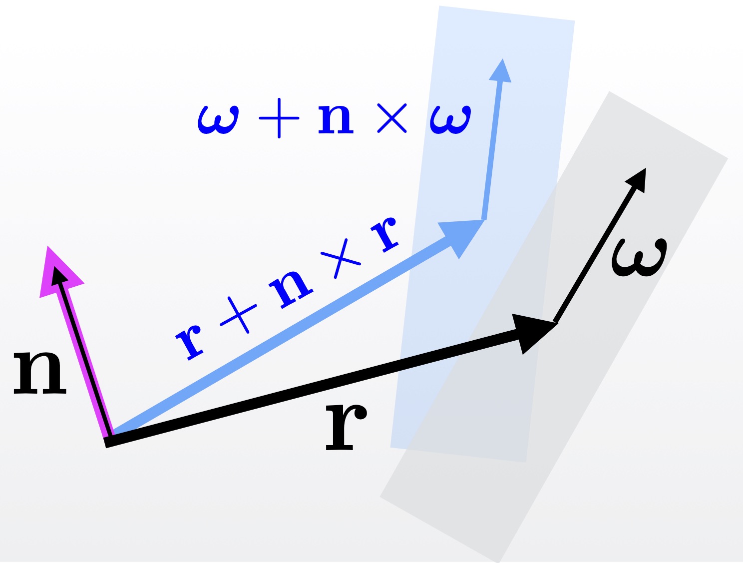
Figure 6: Illustration of the rotation operation of uniaxial particles. The particles (rectangular shapes) at position ${\bf r}$ and with orientation ${\bm{\omega}}$ are shown in original (black) and rotated (blue) configuration, where ${\bf n}$ indicates the rotation axis (direction) and angle (length).

Orbital and spin coupling

The case of rotational symmetry of uniaxial particles is clearly more complex, as both particle coordinates and particle orientations are affected by a global (“rigid”) operation on the entire system, i.e. both positions and orientations are rotated consistently. Noether’s Theorem ensures though that this operation is indeed the fundamental one, and that the physically expected coupling of orbital and spinning effects will naturally and systematically emerge. Here we use (common) terminology for referring to spin as orientation vector rotation (i.e. particle rotation around its center), as opposed to orbital rotation (of position vector) around the origin of position space. Hence all the above considered torques that already occur in systems of spheres are of orbital nature. These of course remain relevant for anisotropic particles, but the nontrivial orientational behaviour of the latter will generate additional spin torques. The global rotation consists of an orbital part, ${\bf r}\to{\bf r}+{\bf n}\times{\bf r}$, and a spin part, ${\bm{\omega}}\to{\bm{\omega}}+{\bf n}\times{\bm{\omega}}$; see Fig. 6 for a graphical representation.

For anisotropic systems the external field naturally acquires dependence on position ${\bf r}$ and orientation ${\bm{\omega}}$, i.e. $V_{\rm ext}({\bf r},{\bm{\omega}})$, where $-\nabla V_{\rm ext}({\bf r},{\bm{\omega}})$ is the external force field as before, and $-{\bm{\omega}}\times\nabla^{\omega}V_{\rm ext}({\bf r},{\bm{\omega}})$ is the external torque field, where $\nabla^{\omega}$ is the derivative with respect to ${\bm{\omega}}$ in orientation space. Hence the induced change of external potential is $\delta V_{\rm ext}({\bf r},{\bm{\omega}})=({\bf n}\times{\bf r})\cdot\nabla V_{\rm ext}+({\bf n}\times{\bm{\omega}})\cdot\nabla^{\omega}V_{\rm ext}$. This change leaves the grand potential $\Omega[V_{\rm ext}]$ invariant, hence $\delta\Omega=\int d{\bf r}d{\bm{\omega}}(\delta\Omega/\delta V_{\rm ext}({\bf r},{\bm{\omega}})){\bf n}\cdot({\bf r}\times\nabla V_{\rm ext}+{\bm{\omega}}\times\nabla^{\omega}V_{\rm ext})=0$, from which we identify the rotational Noether Theorem for the total external torque of anisotropic particles:

$${\bm{\mathcal{T}}}_{\rm ext}^{\rm tot}=-\int d{\bf r}d{\bm{\omega}}\rho({\bf r},{\bm{\omega}})({\bf r}\times\nabla V_{\rm ext}+{\bm{\omega}}\times\nabla^{\omega}V_{\rm ext}) =0.$$ (33)

Differentiation with respect to $V_{\rm ext}({\bf r},{\bm{\omega}})$ yields

$${\bf r}\times\nabla\rho+{\bm{\omega}}\times\nabla^{\omega}\rho=$$ (34)

$$-\negthinspace\int\negthinspace\negthinspace d{\bf r}^{\prime}d{\bm{\omega}}^{\prime}\beta H_{2}({\bf r},{\bm{\omega}},{\bf r}^{\prime},{\bm{\omega}}^{\prime})({\bf r}^{\prime}\times\nabla^{\prime}V_{\rm ext}^{\prime}+{\bm{\omega}}^{\prime}\times\nabla^{\prime\omega}V_{\rm ext}^{\prime}),$$

$$\sum_{\alpha=1}^{n}({\bf r}_{\alpha}\times\nabla_{\alpha}H_{n}+{\bm{\omega}}_{\alpha}\times\nabla^{\omega}_{\alpha}H_{n})=$$

$$-\int d{\bf r}^{\prime}d{\bm{\omega}}^{\prime}\beta V_{\rm ext}^{\prime}({\bf r}^{\prime}\times\nabla^{\prime}H_{n+1}+{\bm{\omega}}^{\prime}\times\nabla^{\prime\omega}H_{n+1}),$$ (35)

where we have used $V_{\rm ext}^{\prime}=V_{\rm ext}({\bf r}^{\prime},{\bm{\omega}}^{\prime})$ as a shorthand, $H_{2}({\bf r},{\bm{\omega}},{\bf r}^{\prime},{\bm{\omega}}^{\prime})=-\delta\rho({\bf r},{\bm{\omega}})/\delta\beta V_{\rm ext}({\bf r}^{\prime},{\bm{\omega}}^{\prime})$ is the density-density correlation function, and its $n$-body version $H_{n}=H_{n}({\bf r}_{1},{\bm{\omega}}_{1}\ldots{\bf r}_{n},{\bm{\omega}}_{n})$ with $H_{n+1}=\delta H_{n}/\delta\beta V_{\rm ext}({\bf r}_{n+1},{\bm{\omega}}_{n+1})$; in (35) the prime refers to the $n+1$th degrees of freedom. Crucially, on all levels of $n$-body correlation functions, the spin and orbital torques remain coupled.

Turning to internal torques, the change of density upon global rotation is $\delta\rho({\bf r},{\bm{\omega}})={\bf n}\cdot({\bf r}\times\nabla\rho+{\bm{\omega}}\times\nabla^{\omega}\rho)$ and the net effect on the excess free energy is $\delta F_{\rm exc}=\int d{\bf r}d{\bm{\omega}}(\delta F_{\rm exc}[\rho]/\delta\rho({\bf r},{\bm{\omega}})){\bf n}\cdot({\bf r}\times\nabla\rho+{\bm{\omega}}\times\nabla^{\omega}\rho)=0$. We hence obtain

$${\bm{\mathcal{T}}}_{\rm ad}^{\rm tot} =\int d{\bf r}d{\bm{\omega}}\rho({\bf r},{\bm{\omega}})({\bf r}\times{\bf f}_{\rm ad}+{\bm{\tau}}_{\rm ad})=0,$$ (36)

where the adiabatic spin torque field is ${\bm{\tau}}_{\rm ad}({\bf r},{\bm{\omega}})=-{\bm{\omega}}\times\nabla^{\omega}\delta F_{\rm exc}[\rho]/\delta\rho({\bf r},{\bm{\omega}})$. From differentiation with respect to $\rho({\bf r},{\bm{\omega}})$ we obtain

$${\bf r}\times{\bf f}_{\rm ad}+{\bm{\tau}}_{\rm ad}=$$

$$\int d{\bf r}^{\prime}d{\bm{\omega}}^{\prime}c_{2}({\bf r},{\bm{\omega}},{\bf r}^{\prime},{\bm{\omega}}^{\prime})({\bf r}^{\prime}\times\nabla^{\prime}\rho^{\prime}+{\bm{\omega}}^{\prime}\times\nabla^{\prime\omega}\rho^{\prime}),$$ (37)

$$\sum_{\alpha=1}^{n}({\bf r}_{\alpha}\times\nabla_{\alpha}c_{n}+{\bm{\omega}}_{\alpha}\times\nabla_{\alpha}^{\omega}c_{n})=$$

$$-\int d{\bf r}^{\prime}d{\bm{\omega}}^{\prime}\rho^{\prime}({\bf r}^{\prime}\times\nabla^{\prime}c_{n+1}+{\bm{\omega}}^{\prime}\times\nabla^{\prime\omega}c_{n+1}),$$ (38)

where $\rho^{\prime}=\rho({\bf r}^{\prime},{\bm{\omega}}^{\prime})$. Multi-body versions of (33) and (36) read as

$$\int d1V_{\text{ext}}(1)\dotsc\int dnV_{\text{ext}}(n)({\bf r}_{\alpha}\times\nabla_{\alpha}+{\bm{\omega}}_{\alpha}\times\nabla_{\alpha}^{\omega})H_{n}=0$$ (39)

and

$$\int d1\rho(1)\dotsc\int dn\rho(n)({\bf r}_{\alpha}\times\nabla_{\alpha}+{\bm{\omega}}_{\alpha}\times\nabla_{\alpha}^{\omega})c_{n}=0.$$ (40)

Here we have used the shorthand notation $1\equiv\textbf{r}_{1},\bm{\omega}_{1}$ etc., and the derivation is analogous to the above rotational case of spherical particles.

The two-body sum rules (34) and (37) are identical to those obtained by Tarazona and Evans tarazona1983 using rotational invariance arguments applied directly to correlation functions. Our methodology not only allows to naturally re-derive their results, but also to identify the full gamut of adiabatic rotatational sum rules, from the global statements (33) and (36) to the infinite hierarchies (35) and (38). (We use notational convention different from Tarazona and Evans tarazona1983 : our $\nabla^{\omega}$ is (only) a partial derivative with respect to ${\bm{\omega}}$, i.e. $\nabla^{\omega}\equiv\partial/\partial{\bm{\omega}}$, whereas their $\nabla_{\omega}\equiv{\bm{\omega}}\times\partial/\partial{\bm{\omega}}$. The modulus is fixed, $|{\bm{\omega}}|=1$, in both versions. Tarazona and Evans tarazona1983 notate $H_{2}$ as $G$ in their (18) and (19).)

Again for each microstate $\sum_{i}({\bf r}_{i}\times\nabla_{i}u+{\bm{\omega}}_{i}\times\nabla_{i}^{\omega}u)=0$ and hence on average ${\bm{\mathcal{T}}}_{\rm int}^{\rm tot}=0$. From the splitting ${\bm{\mathcal{T}}}_{\rm int}^{\rm tot}={\bm{\mathcal{T}}}_{\rm ad}^{\rm tot}+{\bm{\mathcal{T}}}_{\rm sup}^{\rm tot}$, we conclude ${\bm{\mathcal{T}}}_{\rm sup}^{\rm tot}=0$. From rotational invariance of $P_{t}^{\rm exc}[\rho,{\bf J},{\bf J}^{\omega}]$, where ${\bf J}^{\omega}({\bf r},{\bm{\omega}},t)$ is the rotational current krinninger2016prl , against an instantaneous angular “kick” $\delta{\bf J}=(\dot{\bf n}\times{\bf r})\rho$ and $\delta{\bf J}^{\omega}=(\dot{\bf n}\times{\bm{\omega}})\rho$, we find

$${\bm{\mathcal{T}}}_{\rm sup}^{\rm tot}=-\int d{\bf r}d{\bm{\omega}}\rho({\bf r},{\bm{\omega}},t)({\bf r}\times\frac{\delta P_{t}^{\rm exc}}{\delta{\bf J}}+{\bm{\omega}}\times\frac{\delta P_{t}^{\rm exc}}{\delta{\bf J}^{\omega}})=0.$$ (41)

Local sum rules can be obtained straightforwardly by building derivatives with respect to ${\bf J}({\bf r},{\bm{\omega}},t)$ and ${\bf J}^{\omega}({\bf r},{\bm{\omega}},t)$. The result is:

$$\int d{\bf r}_{1}d{\bm{\omega}}_{1}\rho(1)[{\bf r}_{1}\times\delta/\delta{\bf J}(1)+{\bm{\omega}}_{1}\times\delta/\delta{\bf J}^{\omega}(1)]{\sf M}_{n,m}=0.$$ (42)

Here the tensorial equal-time direct correlation functions are defined as ${\sf M}_{n,m}=-\beta\delta^{n+m}P_{t}^{\rm exc}/\delta{\bf J}(1)\ldots\delta{\bf J}(n)\delta{\bf J}^{\omega}(n+1)\ldots{\bf J}^{\omega}(n+m)$, where the roman numerals refer to position, orientation and time $t$ (no index), e.g. $1\equiv{\bf r}_{1},{\bm{\omega}}_{1},t$. We have assumed that all functional derivatives commute.

So far we have restricted ourselves to uniaxial particles. The derived rotational sum rules can be analogously determined for general anisotropic particles with an additional orientation vector $\bm{\varpi}$. This can be done by simply replacing ${\bm{\omega}}\times\nabla^{\omega}\to{\bm{\omega}}\times\nabla^{\omega}+\bm{\varpi}\times\nabla^{\varpi}$, ${\bm{\omega}}\times\frac{\partial}{\partial\textbf{J}^{\omega}}\to{\bm{\omega}}\times\frac{\partial}{\partial\textbf{J}^{\omega}}+\bm{\varpi}\times\frac{\partial}{\partial\textbf{J}^{\varpi}}$ and $\int d\textbf{r}d{\bm{\omega}}\to\int d\textbf{r}d{\bm{\omega}}d\bm{\varpi}$ in (33)-(42). This replacement also affects the adiabatic spin torque field $\tau_{\text{ad}}$ and all one-body field depend additionally to r and ${\bm{\omega}}$ on the orientation $\bm{\varpi}$. For anisotropic particles there exists a more general version of (42) by exchange of ${\sf M}_{n,m}\to{\sf M}_{n,m,l}$, where $l$ denotes the number of functional derivations with respect to the rotational current $\textbf{J}^{\varpi}$. The indices $n$ and $m$ belong to the number of functional derivatives with respect to J and $\textbf{J}^{\omega}$ as before.

Memory invariance

In the above treatment of nonequilibrium situtations we have exploited invariance against an instantaneous transformation applied to the system. As we have shown, the corresponding Noether identities carry imminent physical meaning. These sum rules hold for the nonequilibrium effects that arise from the interparticle interaction, i.e. they constrain superadiabatic forces and torques, as obtained from translation and rotation, respectively. Here we exploit that the corresponding nonequilibrium functional generator $P_{t}^{\rm exc}$ carries further invariances, once one allows the transformation to act also on the history of the system. As we demonstrate in the following, the resulting identities constitute exact constraints on the memory structure that are induced by the coupled interparticle interactions. Recall that a reduced one-body description of a many-body system is generically non-Markovian (i.e. nonlocal in time) zwanzig2001 . The study of memory kernels, often carried out in the framework of generalized Langevin equations, is a topic of significant current research activity lesnicki2016 ; lesnicki2017 ; jung2016 ; jung2017 ; jung2018 ; yeomansreyna2000 ; chavezrojo2006 ; lazarolazaro2017 .

Our approach differs from these efforts in that no a priori generic form of a reduced equation of motion is assumed. Rather our considerations are formally exact and interrelate (and hence constrain) time correlation functions, which are generated from the central nonequilibrium object $P_{t}^{\rm exc}$ via functional differentiation. Very little is known about the memory structure of superadiabatic forces, with exceptions being the NOZ framework brader2013noz ; brader2014noz and the demonstration of the relevance of memory for the observed viscoelasticity of hard sphere liquids treffenstaedt2020shear . Both the Ornstein-Zernike (OZ) and NOZ relations are different from the Noether identities. The former relations are a direct consequence of the generality of the variational principle. Per se, neither the OZ nor the NOZ relations reflect the Noether symmetries.

Recalling the illustrated overview of the different types of shifting in Fig. 1, in the following we treat two further types of invariance transformations: One is the static transformation. This operation is formally analogous to the above equilibrium treatment of the adiabatic state, but it is here carried out in the same way at all times. This static transformation contrasts (and complements) the instantaneous transformation used above for the time-dependent case. The corresponding changes to density and current are graphically illustrated in Fig. 3(b). The second invariance operation is that of memory shifting, where the transformation parameter is taken to be time-dependent, cf. Fig. 3(c) for a graphical representation. For simplicity we restrict ourselves to cases where at both ends of the considered time interval, no shifting occurs (i.e. such that the transformation is the identity at the limiting times).

The static spatial shift consists of $\rho({\bf r},t^{\prime})\to\rho({\bf r}+{\bm{\epsilon}},t^{\prime})$ and ${\bf J}({\bf r},t^{\prime})\to{\bf J}({\bf r}+{\bm{\epsilon}},t^{\prime})$, where the time argument $t^{\prime}$ is arbitrary, and ${\bm{\epsilon}}=\rm const$ characterizes magnitude and direction of the translation, see the illustration in Fig. 3(b). Hence the time derivative $\dot{\bm{\epsilon}}=0$ such that the current does not acquire any displacement contribution, as also $-\dot{\bm{\epsilon}}\rho=0$ at all times. The spatial shift applies to all times $t^{\prime}$ considered, and we can restrict ourselves to $0\leq t^{\prime}\leq t$. Hence the changes in kinematic fields are to first order given by $\delta\rho({\bf r},t^{\prime})={\bm{\epsilon}}\cdot\nabla\rho({\bf r},t^{\prime})$ and $\delta{\bf J}({\bf r},t^{\prime})={\bm{\epsilon}}\cdot\nabla{\bf J}({\bf r},t^{\prime})$. As $P_{t}^{\rm exc}$ originates solely from the interparticle interaction potential, the invariance of $u({\bf r}^{N})$ against the global displacement at all times induces invariance of $P_{t}^{\rm exc}$. Hence $P_{t}^{\rm exc}[\rho,{\bf J}]=P_{t}^{\rm exc}[\rho+\delta\rho,{\bf J}+\delta{\bf J}]=P_{t}^{\rm exc}[\rho,{\bf J}]+\delta P_{t}^{\rm exc}$. Here $\delta P_{t}^{\rm exc}$ indicates the change in superadiabatic free power and due to the invariance $\delta P_{t}^{\rm exc}=0$. On the other hand we can express $\delta P_{t}^{\rm exc}$ via the functional Taylor expansion. To linear order the result consists of two integrals. One integral comes from the time-slice functional derivative at fixed (end) time $t$ and is given by $\int d{\bf r}[(\delta P_{t}^{\rm exc}/\delta\rho)\delta\rho+(\delta P_{t}^{\rm exc}/\delta{\bf J})\cdot\delta{\bf J}]$. The second integral is from a functional derivative at (variable) time $t^{\prime}$, given by $\int_{0}^{t}dt^{\prime}\int d{\bf r}^{\prime}[(\delta P_{t}^{\rm exc}/\delta\rho^{\prime})\delta\rho^{\prime}+(\delta P_{t}^{\rm exc}/\delta{\bf J}^{\prime})\cdot\delta{\bf J}^{\prime}]$, where the prime indicates dependence on arguments ${\bf r}^{\prime}$ and $t^{\prime}$. We then exploit that the displacement ${\bm{\epsilon}}$ of the static shift (which parametrizes the changes in density and in current) is arbitrary. The result is a global nonequilibrium Noether Theorem, given by

$$\int d{\bf r}\Big{(}\frac{\delta P_{t}^{\rm exc}}{\delta\rho}\nabla\rho-{\bf f}_{\rm sup}\cdot\nabla{\bf J}^{\sf T}\Big{)}$$ (43)

$$\quad+\int_{0}^{t}dt^{\prime}\int d{\bf r}^{\prime}\Big{(}\frac{\delta P_{t}^{\rm exc}}{\delta\rho^{\prime}}\nabla^{\prime}\rho^{\prime}+\frac{\delta P_{t}^{\rm exc}}{\delta{\bf J}^{\prime}}\cdot\nabla^{\prime}{\bf J}^{\prime\sf T}\Big{)}=0,$$

where we have used the relationship of the superadiabatic force field to its generator, ${\bf f}_{\rm sup}({\bf r},t)=-\delta P_{t}^{\rm exc}[\rho,{\bf J}]/\delta{\bf J}({\bf r},t)$, the primed symbol $\nabla^{\prime}$ indicates the derivative with respect to ${\bf r}^{\prime}$, and the superscript $\sf T$ denotes the matrix transpose. (In index notation the $k$-component of the vector ${\bf a}\cdot\nabla{\bf b}^{\sf T}$ is $\sum_{k^{\prime}}a_{k^{\prime}}\nabla_{k}b_{k^{\prime}}$.)

Equation (43) constitutes a global identity that links density, current, and superadiabatic force field in a nontrivial spatial and temporal form. As the central variation principle schmidt2013pft allows to vary ${\bf J}({\bf r},t)$ freely, (43) remains true upon building the functional derivative with respect to ${\bf J}({\bf r},t)$. The result is a local identity

$$\beta\nabla{\bf f}_{\rm sup}=$$

$$\int d{\bf r}^{\prime}\big{(}{\bf m}_{2}({\bf r},{\bf r}^{\prime},t)\nabla^{\prime}\rho({\bf r}^{\prime},t)+{\sf M}_{2}({\bf r},{\bf r}^{\prime},t)\cdot\nabla^{\prime}{\bf J}^{\sf T}({\bf r}^{\prime},t)\big{)}$$

$$\quad+\int_{0}^{t}dt^{\prime}\int d{\bf r}^{\prime}\big{(}{\bf m}_{2}({\bf r},t,{\bf r}^{\prime},t^{\prime})\nabla^{\prime}\rho^{\prime}$$ (44)

$$\qquad\qquad\qquad\qquad+{\sf M}_{2}({\bf r},t,{\bf r}^{\prime},t^{\prime})\cdot\nabla^{\prime}{\bf J}^{\prime\sf T}\big{)},$$

where two-body time direct correlation functions occur in vectorial form: ${\bf m}_{2}({\bf r},{\bf r}^{\prime},t)=-\beta\delta^{2}P_{t}^{\rm exc}/\delta{\bf J}({\bf r},t)\delta\rho({\bf r}^{\prime},t)$, ${\bf m}_{2}({\bf r},t,{\bf r}^{\prime},t^{\prime})=-\beta\delta^{2}P_{t}^{\rm exc}/\delta{\bf J}({\bf r},t)\delta\rho({\bf r}^{\prime},t^{\prime})$, as well as in tensorial form: ${\sf M}_{2}({\bf r},{\bf r}^{\prime},t)=-\beta\delta^{2}P_{t}^{\rm exc}/\delta{\bf J}({\bf r},t)\delta{\bf J}({\bf r}^{\prime},t)$, ${\sf M}_{2}({\bf r},t,{\bf r}^{\prime},t^{\prime})=-\beta\delta^{2}P_{t}^{\rm exc}/\delta{\bf J}({\bf r},t)\delta{\bf J}({\bf r}^{\prime},t^{\prime})$. Here we have made the (common) assumption that the second derivatives can be interchanged.

Repeated differentiation of (44) with respect to ${\bf J}({\bf r},t)$ generates a hierarchy,

$$\sum_{\alpha=1}^{n-1}\nabla_{\alpha}{\sf M}_{n-1}({\bf r}^{n-1},t)=$$ (45)

$$\quad\int d{\bf r}_{n}\Big{(}{\bf m}_{n}({\bf r}^{n},t)\nabla_{n}\rho({\bf r}_{n},t)+{\sf M}_{n}({\bf r}^{n},t)\cdot\nabla_{n}{\bf J}({\bf r}_{n},t)^{\sf T}\Big{)}$$

$$\quad+\int_{0}^{t}dt^{\prime}\int d{\bf r}_{n}\Big{(}{\bf m}_{n}({\bf r}^{n-1},t,{\bf r}_{n},t^{\prime})\nabla_{n}\rho({\bf r}_{n},t^{\prime})$$

$$\qquad\qquad\qquad\qquad+{\sf M}_{n}({\bf r}^{n-1},t,{\bf r}_{n},t^{\prime})\cdot\nabla_{n}{\bf J}({\bf r}_{n},t^{\prime})^{\sf T}\Big{)},$$

where the $n$-body equal-time direct correlation functions of rank $n$ are ${\sf M}_{n}({\bf r}^{n},t)=-\beta\delta^{n}P_{t}^{\rm exc}/\delta{\bf J}({\bf r}_{1},t)\ldots\delta{\bf J}({\bf r}_{n},t)$ and ${\bf m}_{n}({\bf r}^{n},t)=-\beta\delta^{n}P_{t}^{\rm exc}/\delta{\bf J}({\bf r}_{1},t)\ldots\delta{\bf J}({\bf r}_{n-1},t)\delta\rho({\bf r}_{n},t)$, where we have used the shorthand ${\bf r}^{n}={\bf r}_{1}\ldots{\bf r}_{n}$. Furthermore at unequal times we have: ${\sf M}_{n}({\bf r}^{n-1},t,{\bf r}_{n},t^{\prime})=-\beta\delta^{n}P_{t}^{\rm exc}/\delta{\bf J}({\bf r}_{1},t)\ldots\delta{\bf J}({\bf r}_{n-1},t)\delta{\bf J}({\bf r}_{n},t^{\prime})$ as a rank $n$ tensor, and also a rank $n-1$ tensor ${\bf m}_{n}({\bf r}^{n-1},t,{\bf r}_{n},t^{\prime})=-\beta\delta^{n}P_{t}^{\rm exc}/\delta{\bf J}({\bf r}_{1},t)\ldots\delta{\bf J}({\bf r}_{n-1},t)\delta\rho({\bf r}_{n},t^{\prime})$.

In the second case, we consider a more general invariance transformation that is obtained by letting the transformation parameter be time-dependent. In this case of time-dependent shifting, we prescribe a displacement vector ${\bm{\epsilon}}(t^{\prime})$ for times $0\leq t^{\prime}\leq t$, i.e. between the intial time, throughout the past and up to the “current” time $t$. We restrict ourselves to vanishing shift at the boundaries of the considered time interval, i.e. ${\bm{\epsilon}}(0)={\bm{\epsilon}}(t)=0$. Due to the overdamped character of the dynamics, its interparticle contributions are unaffected by this transformation, and hence $P_{t}^{\rm exc}$ is invariant. The induced changes that the density and the current acquire arise from shifting their position argument, but the current also acquires an additive shifting current contribution. The latter contribution is analogous to the (sole) effect that is present in the instantaneous shifting, but here applicable at all times (in the considered time interval).

Hence the time-dependent shifting, as illustrated in Fig. 3(c), induces the following changes to the density and the current: $\delta\rho({\bf r}^{\prime},t^{\prime})={\bm{\epsilon}}(t^{\prime})\cdot\nabla^{\prime}\rho({\bf r}^{\prime},t^{\prime})$ and $\delta{\bf J}({\bf r}^{\prime},t^{\prime})={\bm{\epsilon}}(t^{\prime})\cdot\nabla{\bf J}({\bf r}^{\prime},t^{\prime})-\dot{\bm{\epsilon}}(t^{\prime})\rho({\bf r}^{\prime},t^{\prime})$, where $\dot{\bm{\epsilon}}(t^{\prime})=d{\bm{\epsilon}}(t^{\prime})/dt^{\prime}$. Next we can regard $P_{t}^{\rm exc}[\rho+\delta\rho,{\bf J}+\delta{\bf J}]$ as a functional of ${\bm{\epsilon}}(t^{\prime})$ and $\dot{\bm{\epsilon}}(t^{\prime})$. Its invariance amounts to stationarity, i.e. vanishing first functional derivative, with respect to the displacement. This problem, in particular for the present case of fixed boundary values, amounts to one of the most basic problems in the calculus of variations. It is realized, e.g., in the determination of catenary curves and indeed, in Hamilton’s principle of classical mechanics. Exploiting the corresponding Euler-Lagrange equation leads to

$$\frac{d}{dt^{\prime}}\int d{\bf r}^{\prime}{\bf m}^{\prime}_{1}\rho^{\prime}+\int d{\bf r}^{\prime}{\bf m}_{1}^{\prime}\cdot\nabla^{\prime}{\bf J}^{\prime\sf T}+\int d{\bf r}^{\prime}m_{1}^{\prime}\nabla^{\prime}\rho^{\prime} =0,$$ (46)

where the one-body time direct correlation functions are ${\bf m}^{\prime}_{1}({\bf r}^{\prime},t^{\prime},t)=-\beta\delta P_{t}^{\rm exc}/\delta{\bf J}({\bf r}^{\prime},t^{\prime})$ and $m^{\prime}_{1}({\bf r}^{\prime},t^{\prime},t)=-\beta\delta P_{t}^{\rm exc}/\delta\rho({\bf r}^{\prime},t^{\prime})$. Differentiation with respect to ${\bf J}({\bf r},t)$ yields again a local memory identity.

Conclusions

We have demonstrated that Noether’s Theorem for exploiting symmetry in a variational context has profound implications for Statistical Physics. Known sum rules can be derived with ease and powerfully generalized to full infinite hierarchies, to the rotational case, and to time-dependence in nonequilibrium. Recall the selected applications xu2008 ; brader2008precursor ; walz2010 ; haering2015 ; haering2020phd ; bryk1997 ; tejero1985 ; iatsevitch1997 ; kasch1993 ; henderson1984 ; mandal2017 of the equilibrium sum rules, as we have laid out in the introduction. For the time-dependent case, we envisage similar insights from using the newly formulated nonequilibrium sum rules in investigations of e.g the dynamics of freezing, of liquid crystal flow, and of driven fluid interfaces. On the conceptual level, Noether’s Theorem assigns a clear meaning and physical interpretation to all resulting identities, as being generated from an invariance property of an underlying functional generator. Although the symmetry operation that we considered are simplistic, and only their lowest order in a power series expansion needs to be taken into account, a significantly complex body of sum rules naturally emerges. Hence the application of Noether’s Theorem is significantly deeper than mere exploiting of symmetries of arguments of correlation functions, i.e. that the direct correlation function $c_{2}({\bf r},{\bf r}^{\prime})$ in bulk fluids depends solely on $|{\bf r}-{\bf r}^{\prime}|$. Rather, as governed by functional calculus, coupling of different levels of correlation functions occurs.

Crucially, the Noether sum rules are different from the variational principle, as embodied in the Euler-Lagrange equation. On the formal level, the difference is that the Euler-Lagrange equation (both of DFT and of PFT) is a formally closed equation on the one-body level. In contrast, the Noether rules couple $n$- and $(n+1)$-body correlation functions, hence they are of genuine hierarchical nature. They also describe different physics, as the Euler-Lagrange equation expresses a chemical potential equilibrium in DFT and the local force balance relationship in PFT. In contrast, the Noether identities stem from the symmetry properties of the respective underlying physical system.

The standard DFT approximations, ranging from simple local, square-gradient, and mean-field functional to more sophisticated weighted-density-schemes including fundamental measure theory satisfy the internal force relationships. This can be seen straightforwardly by observing that these functionals do satisfy global translation invariance. (The value of the free energy is independent of the choice of coordinate origin.) All higher-order Noether identities are then automatically satisfied, as these inherit the correct symmetry properties from the generating (excess free energy) functional. Our formalism hence provides a concrete reason, over mere empirical experience, why the practitioners’ choices for approximate functionals are sound. The situation for more complex DFT schemes could potentially be different though. As soon as, say, self-consistency of some form is imposed, or coupling to auxiliary field comes into play, it is easy to imagine that the Noether identities help in restricting choices in the construction of such approximation schemes.

The sum rules imposed by the three types of dynamical displacements are satisfied within the velocity gradient form of the power functional delasheras2018velocityGradient ; delasheras2020prl . It is straightforward to see that the functional is independent of the coordinate origin (static shifting). For the cases of dynamical shifting, the invariance of the functional stems from invariance of the velocity field against shifting. For both instantaneous and memory shifting, the velocity gradient remains invariant under the displacement.

We envisage that the higher than two-body Noether identities can facilitate the construction of advanced liquid state/density functional approximations. Such work should surely be highly challenging. In the context of fundamental measure theory (see e.g. the work by Roth roth2010review for an enlightening review) it is worth recalling that in Rosenfeld’s original 1989 paper rosenfeld1989 , he calculated the three-body direct correlation function from his then newly proposed functional. The result for the corresponding three-body pair correlations compared favourably against simulation data. Furthermore, the recent insights into two-body correlations in inhomogeneous liquids tschopp2021 and crystals oettel2021 demonstrates that working with higher-body correlation functions is feasible.

In future work it would be very beneficial to bring together the Noether identities with the nonequilibrium Ornstein-Zernike relations brader2013noz ; brader2014noz , in order to aid construction of new dynamical approximations. One could exploit the rotational invariance of the superadiabatic excess power functional $P_{t}^{\rm exc}$ to gain deeper insights in its memory structure and also generalize the translational memory relations (43)-(46) to anisotropic particles. It would be highly interesting to apply (49) to the recently obtained direct correlation function of the hard sphere crystal. This would allow to investigate whether Triezenberg and Zwanzig’s concept that they originally developed for the free gas-liquid interface applies to the also self-sustained density inhomogeneity in a solid. Furthermore, addressing further cases of self motility farage2015 ; paliwal2018 ; paliwal2017activeLJ , including active freezing turci2020 ; geissler2021 , as well as further types of time evolution, such as molecular dynamics or quantum mechanics should be interesting. This is feasible, as the Noether considerations are not restricted to overdamped classical systems, as (formal) power functional generators exist for quantum schmidt2015qm and classical Hamiltonian schmidt2018md many-body systems. On the methodological side, besides power functional theory, our framework could be complemented by e.g. mode-coupling theory and Mori-Zwanzig techniques janssen2018 , as well as approaches beyond that fuchs2020. Given that the equilibrium force sum rules are crucial in the description of crystal walz2010 ; haering2015 and liquid crystal haering2020phd excitations, the study of such systems under drive is a further exciting prospect.

Methods

Relationship to classical results

We give an overview of how the Noether sum rules relate to previously known results. The famous LMBW-equation was derived independently by Lovett, Mou, and Buff lovett1976 and by Wertheim wertheim1976 and reads

$$\nabla\ln\rho(\textbf{r})+\beta\nabla V_{\text{ext}}(\textbf{r})=\int d\textbf{r}^{\prime}c_{2}(\textbf{r},\textbf{r}^{\prime})\nabla^{\prime}\rho(\textbf{r}^{\prime}).$$ (47)

We can conclude that (47) is a combination of the local internal Noether sum rule (7) for translational symmetry and the equilibrium Euler-Lagrange equation $c_{1}(\textbf{r})=\ln\rho(\textbf{r})+\beta\nabla V_{\text{ext}}(\textbf{r})-\beta\mu$, where $\mu$ indicates the chemical potential. LMBW also derived a lesser known external relation, which is equivalent to (47) and reads

$$\nabla\rho(\textbf{r})+\beta\rho(\textbf{r})\nabla V_{\text{ext}}(\textbf{r})=$$

$$\qquad\int d\textbf{r}^{\prime}(g(\textbf{r},\textbf{r}^{\prime})-1)\rho(\textbf{r})\rho(\textbf{r}^{\prime})\nabla^{\prime}V_{\text{ext}}(\textbf{r}^{\prime}).$$ (48)

We find that (48) contains the local external Noether sum rule (3) along with the relation $H_{2}(\textbf{r},\textbf{r}^{\prime})=(g(\textbf{r},\textbf{r}^{\prime})-1)\rho(\textbf{r})\rho^{\prime}(\textbf{r}^{\prime})+\rho(\textbf{r})\delta(\textbf{r}-\textbf{r}^{\prime})$ hansen2013 .

The Triezenberg-Zwanzig equation TZ1972 holds for vanishing external potential $V_{\text{ext}}(\textbf{r})=0$ and is given by

$$\nabla\ln\rho(\textbf{r})=\int d\textbf{r}^{\prime}c_{2}(\textbf{r},\textbf{r}^{\prime})\nabla^{\prime}\rho(\textbf{r}^{\prime}).$$ (49)

Originally (49) was derived for the free liquid-vapour interface in a parallel geometry. We find that the relation consists of the local internal Noether sum rule (7) and the equilibrium Euler-Lagrange equation. The LMBW equation (48) reduces to the Triezenberg-Zwanzig equation (49) for cases of $V_{\text{ext}}(\textbf{r})=0$.

Another related equation is the first member of the Yvon-Born-Green (YBG) hierarchy yvon; borngreen,

$$\rho(\nabla\ln\rho(\textbf{r})+\beta\nabla V_{\text{ext}}(\textbf{r}))=$$

$$\qquad-\beta\int d\textbf{r}^{\prime}g(\textbf{r},\textbf{r}^{\prime})\rho(\textbf{r})\rho(\textbf{r}^{\prime})\nabla\phi(|\textbf{r}-\textbf{r}^{\prime}|),$$ (50)

where $\phi(r)$ denotes the interparticle pair potential as before. Although (50) has a similar structure as the LMBW equation, it is not based on symmetry or Noether arguments but arises from integration out of degrees of freedom. If one would like to include the translational symmetry one can simply replace the left hand side of (50) with the right hand side of the LMBW equation (47), which leads to

$$\int d\textbf{r}^{\prime}c_{2}(\textbf{r},\textbf{r}^{\prime})\nabla^{\prime}\rho(\textbf{r}^{\prime})=-\beta\int d\textbf{r}^{\prime}g(\textbf{r},\textbf{r}^{\prime})\rho(\textbf{r}^{\prime})\nabla\phi(|\textbf{r}-\textbf{r}^{\prime}|).$$ (51)

Some of the here derived sum rules are rederivations of known relations. We reiterate the relationships. In his overview Baus baus1984 showed that in equilibrium the total external (2) and internal (6) force vanish and derived the corresponding local hierarchies (3), (4) and (7), (8). Similar sum rules baus1984 hold for the external (22) and internal (25) total torques and their corresponding hierarchies (23), (24) and (26), (27). Tarazona and Evans tarazona1983 generalized these equations for uniaxial particles and derived the first order of the external (34) and internal (37) hierarchies due to rotations.

To the best of our knowledge the hierarchies of global Noether sum rules, such as (5), (9), (28), and (29), have not been determined previously. Furthermore the global external (33) and internal (36) Noether sum rules for uniaxial colloids and their corresponding hierarchies (35) and (38) (with exception of the first order) are reported here for the first time. As the considerations in the literature focused on equilibrium, all our nonequilibrium relations, as e.g. (11)-(13) and especially the ones including memory (43)-(46) have not been found before.

References

Invariante Variationsprobleme. E. Noether, Nachr. d. König. Gesellsch. d. Wiss. zu Göttingen, Math.-Phys. Klasse, 235 (1918). English translation by M. A. Tavel: Invariant variation problems. Transp. Theo. Stat. Phys. 1, 186 (1971); for a version in modern typesetting see: Frank Y. Wang, arXiv:physics/0503066v3 (2018).

For a description of many insightful and pedagogical examples and applications, see: D. E. Neuenschwander, Emmy Noether’s Wonderful Theorem (Johns Hopkins University Press, Baltimore, 2011).

E. Noether’s discovery of the deep connection between symmetries and conservation laws. N. Byers, arXiv:physics/9807044 (1998).

J. S. Rowlison and B. Widom, Molecular Theory of Capillarity (Dover, New York, 2002).

The thermodynamic theory of capillarity under the hypothesis of a continuous variation of density. J. D. van der Waals, Z. Phys. Chem. 13, 657 (1894); English translation by J. S. Rowlinson, J. Stat. Phys. 20, 197 (1979).

Applications of noether’s theorem to inhomogeneous fluids. J. Kerins and M. Boiteux, Physica A 117, 575 (1983).

Torque balance at a line of contact. D. J. Bukman, Physica A 319, 151 (2003).

Thermodynamic properties of inhomogeneous fluids. M. Boiteux and J. Kerins, Physica A 121, 399 (1983).

The nature of the liquid-vapour interface and other topics in the statistical mechanics of non-uniform, classical fluids. R. Evans, Adv. Phys. 28, 143 (1979).

The structure of the liquid–vapor interface. R. A. Lovett, C. Y. Mou, and F. P. Buff, J. Chem. Phys. 65, 570 (1976).

Correlations in the liquid–vapor interface. M. S. Wertheim, J. Chem. Phys. 65, 2377 (1976).

Emergence of periodic density patterns. R. F. Kayser and H. J. Raveché, Phys. Rev. B 22, 424 (1980).

Broken symmetry and invariance properties of classical fluids. M. Baus, Mol. Phys. 51, 211 (1984).

Examples of the construction of integral equations in equilibrium statistical mechanics from invariance principles. R. Lovett and F. P. Buff, Physica A 172, 147 (1991).

A direct derivation of the profile equations of Buff-Lovett-Mou-Wertheim from the Born-Green-Yvon equations for a non-uniform equilibrium fluid. M. Baus and R. Lovett, Physica A 181, 329 (1992).

On the validity of certain integro-differential equations for the density-orientation profile of molecular fluid interfaces. P. Tarazona and R. Evans, Chem. Phys. Lett. 97, 279 (1983).

Structure of nonuniform molecular fluids – integrodifferential equations for the density-orientation profile. K. E. Gubbins, Chem. Phys. Lett. 76, 329 (1980).

J. P. Hansen and I. R. McDonald, Theory of Simple Liquids, 4th ed. (Academic Press, London, 2013).

New developments in classical density functional theory. R. Evans, M. Oettel, R. Roth, and G. Kahl, J. Phys.: Condens. Matter 28, 240401 (2016).

Fundamental measure theory for hard-sphere mixtures: a review. R. Roth, J. Phys.: Condens. Matt. 22, 063102 (2010).

Scalar fundamental measure theory for hard spheres in three dimensions: Application to hydrophobic solvation. M. Levesque, R. Vuilleumier, and D. Borgis, J. Chem. Phys. 137, 034115 (2012).

Molecular density functional theory of water describing hydrophobicity at short and long length scales. G. Jeanmairet, M. Levesque, and D. Borgis, J. Chem. Phys. 139, 154101 (2013).

Commentary: Playing the long game wins the cohesion–adhesion rivalry. R. C. Remsing, Proc. Nat. Acad. Sci. 116, 23874 (2019).

A unified description of hydrophilic and superhydrophobic surfaces in terms of the wetting and drying transitions of liquids. R. Evans, M. C. Stewart, and N. B. Wilding, Proc. Nat. Acad. Sci. 116, 23901 (2019).

Quantifying density fluctuations in water at a hydrophobic surface: evidence for critical drying. R. Evans and N. B. Wilding, Phys. Rev. Lett. 115, 016103 (2015).

Critical drying of liquids. R. Evans, M. C. Stewart, and N. B. Wilding, Phys. Rev. Lett. 117, 176102 (2016).

Solvent fluctuations around solvophobic, solvophilic, and patchy nanostructures and the accompanying solvent mediated interactions. B. Chacko, R. Evans, and A. J. Archer, J. Chem. Phys. 146, 124703 (2017).

Atomically resolved three-dimensional structures of electrolyte aqueous solutions near a solid surface. D. Martin-Jimenez, E. Chacón, P. Tarazona, and R. Garcia, Nat. Comms. 7, 12164 (2016).

Density functional analysis of atomic force microscopy in a dense fluid. J. Hernández-Muñoz, E. Chacón, and P. Tarazona, J. Chem. Phys. 151, 034701 (2019).

Deconstructing temperature gradients across fluid interfaces: the structural origin of the thermal resistance of liquid-vapor interfaces. J. Muscatello, E. Chacón, P. Tarazona, and F. Bresme, Phys. Rev. Lett. 119, 045901 (2017).

A density functional theory of one- and two-layer freezing in a confined colloid system. X. Xu and S. A. Rice, Proc. R. Soc. A 464, 65 (2008).

Structural precursor to freezing: An integral equation study. J. M. Brader, J. Chem. Phys. 128, 104503 (2008).

Displacement field and elastic constants in nonideal crystals. C. Walz and M. Fuchs, Phys. Rev. B 81, 134110 (2010).

Coarse-grained density and compressibility of nonideal crystals: General theory and an application to cluster crystals. J. M. Häring, C. Walz, G. Szamel, and M. Fuchs, Phys. Rev. B 92, 184103 (2015).

Microscopically founded elasticity theory for defect-rich systems of anisotropic particles. J. M. Häring, Ph.D. Thesis, Universität Konstanz (2020).

A fluid in contact with a semipermeable surface: Second-order integral equation approach. P. Bryk, D. Henderson, and S. Sokolowski, J. Chem. Phys. 107, 3333 (1997).

Viscoelastic surface waves and the surface structure of liquids. C. F. Tejero and M. Baus, Mol. Phys. 54, 1307 (1985).

Density profiles at liquid-vapor and liquid-liquid interfaces: An integral equation study. S. Iatsevitch and F. Forstmann, J. Chem. Phys. 107, 6925 (1997).

An orientational instability and the liquid-vapor interface of a dipolar hard sphere fluid. M. Kasch and F. Forstmann, J. Chem. Phys. 99, 3037 (1993).

On the interface between a fluid and a planar wall. J. R. Henderson and F. van Swol, Mol. Phys. 51, 991 (1984).

Nonergodicity parameters of confined hard-sphere glasses. S. Mandal, S. Lang, V. Botan, and T. Franosch, Soft Matter 13, 6167 (2017).

Effective interactions in active Brownian suspensions, T. F. F. Farage, P. Krinninger, and J. M. Brader, Phys. Rev. E 91, 042310 (2015).

Chemical potential in active systems: predicting phase equilibrium from bulk equations of state? S. Paliwal, J. Rodenburg, R. van Roij, and M. Dijkstra, New J. Phys. 20 015003 (2018).

Non-equilibrium surface tension of the vapour-liquid interface of active Lennard- Jones particles. S. Paliwal, V. Prymidis, L. Filion, and M. Dijkstra, J. Chem. Phys. 147, 084902 (2017).

Topological protection of multiparticle dissipative transport. J. Loehr, M. Loenne, A. Ernst, D. de las Heras, and T. M. Fischer, Nat. Commun. 7, 11745 (2016).

Colloidal topological insulators. J. Loehr, D. de las Heras, A. Jarosz, M. Urbaniak, F. Stobiecki, A. Tomita, R. Huhnstock, I. Koch, A. Ehresmann, D. Holzinger, and T. M. Fischer, Comms. Phys. 1, 4 (2018).

Hard topological versus soft geometrical magnetic particle transport. A. M. E. B. Rossi, J. Bugase, T. Lachner, A. Ernst, D. de las Heras, and T. M. Fischer, Soft Matter 15, 8543 (2019).

Power functional theory for Brownian dynamics. M. Schmidt and J. M. Brader, J. Chem. Phys. 138, 214101 (2013).

Superadiabatic forces in Brownian many-body dynamics. A. Fortini, D. de las Heras, J. M. Brader, and M. Schmidt, Phys. Rev. Lett. 113, 167801 (2014).

Nonequilibrium phase behaviour from minimization of free power dissipation. P. Krinninger, M. Schmidt, and J. M. Brader, Phys. Rev. Lett. 117, 208003 (2016).

Non-negative interfacial tension in phase-separated active Brownian particles. S. Hermann, D. de las Heras, and M. Schmidt, Phys. Rev. Lett. 123, 268002 (2019).

Phase coexistence of active Brownian particles. S. Hermann, P. Krinninger, D. de las Heras, and M. Schmidt, Phys. Rev. E 100, 052604 (2019).

Active interface polarization as a state function. S. Hermann and M. Schmidt, Phys. Rev. Research 2, 022003(R) (2020).

Velocity gradient power functional for Brownian dynamics. D. de las Heras and M. Schmidt, Phys. Rev. Lett. 120, 028001 (2018).

Structural nonequilibrium forces in driven colloidal systems. N. C. X. Stuhlmüller, T. Eckert, D. de las Heras, and M. Schmidt, Phys. Rev. Lett. 121, 098002 (2018).

Flow and structure in nonequilibrium Brownian many-body systems. D. de las Heras and M. Schmidt, Phys. Rev. Lett. 125, 018001 (2020).

Nonequilibrium Ornstein-Zernike relation for Brownian many-body dynamics. J. M. Brader and M. Schmidt, J. Chem. Phys. 139, 104108 (2013).

Dynamic correlations in Brownian many-body systems. J. M. Brader and M. Schmidt, J. Chem. Phys. 140, 034104 (2014).

The influence of accidental deviations of density on the equation of state. L. S. Ornstein and F. Zernike, Proc. Acad. Sci. Amsterdam 17, 793 (1914); this article is reprinted in H. Frisch and J. L. Lebowitz, The Equilibrium Theory of Classical Fluids (Benjamin, New York, 1964).

(Infinite) Boundary corrections for the LMBW-Equations and the TZ-Formula of surface tension in the presence of spontaneous symmetry breaking. M. Requardt and H. J. Wagner, Physica A 154, 183 (1988).

Active particles bound by information flows. U. Khadka, V. Holubec, H. Yang, F. Cichos, Nat. Commun. 9, 3864 (2018).

Theory for controlling individual self-propelled micro-swimmers by photon nudging I: directed transport. M. Selmke, U. Khadka, A. P. Bregulla, F. Cichos, and H. Yang, Phys. Chem. Chem. Phys. 20, 10502 (2018).

Theory for controlling individual self-propelled micro-swimmers by photon nudging II: confinement. M. Selmke, U. Khadka, A. P. Bregulla, F. Cichos, and H. Yang, Phys. Chem. Chem. Phys. 20, 10521 (2018).

Stochastic localization of microswimmers by photon nudging. A. P. Bregulla, H. Yang, and F. Cichos, ACS Nano 8, 6542 (2014).

Harnessing thermal fluctuations for purposeful activities: the manipulation of single micro-swimmers by adaptive photon nudging. B. Qian, D. Montiel, A. Bregulla, F. Cichos, and H. Yang, Chem. Sci. 4, 1420 (2013).

How Activity Landscapes Polarize Microswimmers without Alignment Forces. N. A. Söker, S. Auschra, V. Holubec, K. Kroy, and F. Cichos, Phys. Rev. Lett.126, 228001 (2021).

Polarization-density patterns of active particles in motility gradients. S. Auschra, V. Holubec, N. A. Söker, F. Cichos, and K. Kroy, Phys. Rev. E 103, 062601 (2021).

Ideal bulk pressure of active Brownian particles. T. Speck and R. L. Jack, Phys. Rev. E 93, 062605 (2016).

Swim pressure: stress generation in active matter. S. C. Takatori, W. Yan, and J. F. Brady, Phys. Rev. Lett. 113, 028103 (2014).

Aggregation and segregation of confined active particles. X. Yang, M. L. Manning, and M. C. Marchetti, Soft Matter 10, 6477 (2014).

Virial pressure in systems of spherical active Brownian particles. R. G. Winkler, A. Wysocki, and G. Gompper, Soft Matter 11, 6680 (2015).

Pressure and Phase Equilibria in Interacting Active Brownian Spheres. A. P. Solon, J. Stenhammar, R. Wittkowski, M. Kardar, Y. Kafri, M. E. Cates, and J. Tailleur, Phys. Rev. Lett. 114, 198301 (2015).

Chemical potential in active systems: predicting phase equilibrium from bulk equations of state? S. Paliwal, J. Rodenburg, René van Roij, and M. Dijkstra, New J. Phys. 20, 015003 (2018).

Floating nematic phase in colloidal platelet-sphere mixtures. D. de las Heras, N. Doshi, T. Cosgrove, J. Phipps, D. I. Gittins, J. S. van Duijneveldt, and M. Schmidt, Sci. Rep. 2, 789 (2012).

The phase stacking diagram of colloidal mixtures under gravity. D. de las Heras and M. Schmidt, Soft Matter 9, 98636 (2013).

Sedimentation stacking diagram of binary colloidal mixtures and bulk phases in the plane of chemical potentials. D. de las Heras and M. Schmidt, J. Phys.: Condens. Matter 27, 194115 (2015).

The role of sample height in the stacking diagram of colloidal mixtures under gravity. T. Geigenfeind and D. de las Heras, J. Phys.: Condens. Matter 29, 064006 (2017).

Active colloidal suspensions exhibit polar order under gravity. M. Enculescu and H. Stark, Phys. Rev. Lett. 107, 058301 (2011).

Active ideal sedimentation: exact two-dimensional steady states. S. Hermann and M. Schmidt, Soft Matter 14, 1614 (2018).

Dynamics of sedimenting active Brownian particles. J. Vachier and M. G. Mazza, Eur. Phys. J. E 42, 11 (2019).

Active Brownian particles and run-and-tumble particles: A comparative study. A. P. Solon, M. E. Cates, and J. Tailleur, Eur. Phys. J. Spec. Top. 224, 1231 (2015).

Active particles under confinement: aggregation at the wall and gradient formation inside a channel. C. F. Lee, New J. Phys. 15, 055007 (2013).

R. Zwanzig, Nonequilibrium Statistical Mechanics (Oxford University Press, Oxford, 2001).

Molecular hydrodynamics from memory kernels. D. Lesnicki, R. Vuilleumier, A. Carof, and B. Rotenberg, Phys. Rev. Lett. 116, 147804 (2016).

Microscopic flow around a diffusing particle. D. Lesnicki and R. Vuilleumier, J. Chem. Phys. 147, 094502 (2017).

Computing bulk and shear viscosities from simulations of fluids with dissipative and stochastic interactions. G. Jung and F. Schmid, J. Chem. Phys. 144, 204104 (2016).

Iterative reconstruction of memory kernels. G. Jung, M. Hanke, and F. Schmid, J. Chem. Theo. Comput. 13, 2481 (2017).

Generalized Langevin dynamics: construction and numerical integration of non-Markovian particle-based models. G. Jung, M. Hanke, and F. Schmid, Soft Matter 14, 9368 (2018).

Overdamped van Hove function of colloidal suspensions. L. Yeomans-Reyna, and M. Medina-Noyola, Phys. Rev. E 62, 3382 (2000).

Van Hove function of colloidal mixtures: Exact results. M. A. Chávez-Rojo, and M. Medina-Noyola, Physica A 366, 55 (2006).

Self-consistent generalized Langevin equation theory of the dynamics of multicomponent atomic liquids. E. Lázaro-Lázaro, P. Mendoza-Méndez, L. F. Elizondo-Aguilera, J. A. Perera-Burgos, P. E. Ramirez-González, G. Pérez-Angel, R. Castaneda-Priego, and M. Medina-Noyola, J. Chem. Phys. 146, 184506 (2017).

Memory-induced motion reversal in Brownian liquids. L. L. Treffenstädt and M. Schmidt, Soft Matter 16, 1518 (2020).

Free-energy model for the inhomogeneous hard-sphere fluid mixture and density-functional theory of freezing. Y. Rosenfeld, Phys. Rev. Lett. 63, 9 (1989).

Fundamental measure theory of inhomogeneous two-body correlation functions. S. M. Tschopp and J. M. Brader, Phys. Rev. E 103, 042103 (2021).

The direct correlation function of a crystalline solid. S.-C. Lin, M. Oettel, J. M. Häring, R. Haussmann, M. Fuchs, and G. Kahl, Phys. Rev. Lett. (to appear), arXiv:2104.11558 (2021).

Phase separation and multibody effects in three-dimensional active Brownian particles. F. Turci and N. B. Wilding, Phys. Rev. Lett. 126, 038002 (2021).

Phase diagram of active Brownian spheres: crystallization and the metastability of motility-induced phase separation. A. K. Omar, K. Klymko, T. GrandPre, and P. L. Geissler, Phys. Rev. Lett. 126, 188002 (2021).

Quantum power functional theory for many-body dynamics. M. Schmidt, J. Chem. Phys. 143, 174108 (2015).

Power functional theory for Newtonian many-body dynamics. M. Schmidt, J. Chem. Phys. 148, 044502 (2018).

Mode-coupling theory of the glass transition: A primer. L. M. C. Janssen, Front. Phys. 6, 97 (2018).