On the spatial extent of localized eigenfunctions for random Schrödinger operators

Abstract.

The present paper is devoted to new, improved bounds for the eigenfunctions of random operators in the localized regime. We prove that, in the localized regime with good probability, each eigenfunction is exponentially decaying outside a ball of a certain radius, which we call the “localization onset length”. For $\ell>0$ large, we count the number of eigenfunctions having onset length larger than $\ell$ and find it to be smaller than $\exp(-C\ell)$ times the total number of eigenfunctions in the system. Thus, most eigenfunctions localize on finite size balls independent of the system size.

1. Introduction

Single particle Anderson localization is extremely well studied in both the physics and mathematics literature. The phenomenon was first identified by Anderson in 1958, who argued that for tight-binding models with sufficiently strong on-site disorder the eigenstates corresponding to a spectral band may be exponentially localized in space [4]. As was later clarified in the mathematics literature [14, 10, 9, 21], this can be understood as almost-sure pure-point spectrum for the corresponding Hamiltonians along with exponential decay of the corresponding eigenfunctions.

Extensive random systems, with sufficient decorrelation between distant regions, are characterized by the dictum “anything that can happen does happen, infinitely often.” In particular, there are arbitrarily large regions exhibiting atypical local behavior. As a consequence, among the eigenfunctions of a random Hamiltonian exhibiting Anderson localization, one expects to find examples which fail to decay over arbitrarily large scales. For instance an eigenfunction may have a majority of its mass in a region where the Hamiltonian is extremely close to a periodic operator over a box of size $\ell$. Over this box, the eigenfunction will be close to an eigenfunction of the corresponding periodic operator, which is extended over the whole box. Although the eigenfunction will eventually decay exponentially, we may need to look far from its center of localization to observe that decay.

In [7], del Rio, Jitomirskaya, Last and Simon observed that dynamical localization is related to spectral localization through a quantitative bound allowing for the rare a-typical behavior described in the previous paragraph. They noted that, for various models for which localization had been proved, the eigenfunctions were shown to have the following strong property, which they dubbed Semi-Uniformly Localized Eigenfunctions or SULE. An operator has a SULE basis if there is a basis $\varphi_{j},$ $j=1,\ldots,\infty$, of eigenfunctions such that for some $\mu>0$ it holds that

(1.1) $$|\varphi_{j}(x)|\ \leq\ C_{\epsilon}e^{\epsilon|x_{j}|}e^{-\mu|x-x^{(j)}|}$$

where $x^{(j)}$ is a localization center for $\psi_{j}$ and $C_{\epsilon}$ is finite for any $\epsilon>0$. In the random context, the decay constant $\mu$ is assumed not to depend on the realization of the disorder, but the constants $C_{\epsilon}$ may be disorder dependent (although finite almost surely). In subsequent work, it was observed that in many cases one may obtain the sharper bound

(1.2) $$|\varphi_{j}(x)|\ \leq\ C_{\nu}(1+|x^{(j)}|)^{\nu}e^{-\mu|x-x^{(j)}|}$$

for $\nu>\nicefrac{{d}}{{2}}$, with $C_{\nu}$ finite almost surely.

The exponentially growing prefactor in (1.1) is relevant only if $|x-x^{(j)}|>\frac{\epsilon}{\mu}|x^{(j)}|+\log C_{\omega;\epsilon}$; for $x$ closer to $x^{(j)}$, we may replace (1.1) by the simple bound $|\psi_{j}(x)|\leq 1$ valid for any $\ell^{2}$-normalized lattice function. Thus the presence of the prefactor $e^{\epsilon|x^{(j)}|}$ accounts for the possibility, at large scales, that some eigenfunctions may be extended over a large region outside of which exponential decay sets in. However, this possibility is dealt with coarsely in eq. (1.1), since all eigenfunctions with localization centers far from the origin are painted with the same brush. In fact, one expects many of these eigenfunctions to satisfy a better bound, without the prefactor $e^{\epsilon|x^{(j)}|}$.

Our main goal here is to present a refinement of SULE that manifests the fact that most eigenfunctions, wherever they may be localized, are well localized on a region of size $O(1)$. Roughly, we accomplish this by associating to each eigenfunction a “localization volume”, which informally is the size of the smallest lattice box outside of which the eigenfunction exhibits exponential decay. Our main result is the following improvement of (1.1), which we prove holds throughout the localization regime of the Anderson model:

there is $\mu>0$ such that, with probability one, the eigenfunctions of the Anderson model satisfy

(1.3) $$|\varphi_{j}(x)|\ \leq\|\varphi_{j}\|_{\infty}\ e^{-\mu(|x-x^{(j)}|-\ell_{j})_{+}},$$

where $x^{(j)}\in{\mathbb{Z}}^{d}$, $\ell_{j}\geq 0$, $(a)_{+}=\nicefrac{{(|a|+a)}}{{2}}$ denotes the positive part and $\displaystyle\|\varphi_{j}\|_{\infty}=\max_{x\in{\mathbb{Z}}^{d}}|\varphi_{j}(x)|$; furthermore, there are $C>0$ and $\ell_{0}>0$, such that, for $\ell>\ell_{0}$, one has

(1.4) $$\limsup_{L\rightarrow\infty}\frac{\#\left\{j\ \middle|\ |x^{(j)}|\leq L\quad\text{and}\quad\ell_{j}\geq\ell\right\}}{(2L+1)^{d}}\ \leq\ e^{-C\ell}.$$

The key point here is (1.4), which bounds the number of eigenfunctions $\psi_{j}$ for which the length $\ell_{j}$ is large. We emphasize that $\ell_{j}$ is not the “localization length” of $\phi_{j}$. Indeed, the localization length is a disorder independent function of the energy of the eigenfunction. It is the scale over which exponential decay occurs in the tail of the eigenfunction, and is bounded by $\nicefrac{{1}}{{\mu}}$ for all functions in a SULE basis. Rather, $\ell_{j}$ is the length scale at which localization phenomenon sets in for the particular eigenfunction $\phi_{j}$. For this reason, we refer to $\ell_{j}$ as the localization onset length, or onset length, of $\phi_{j}$. As will be clear from the proof, eigenfunctions $\phi_{j}$ with large onset lengths $\ell_{j}$ are associate to rare behavior over the region $|x-x_{E}|\leq\ell_{j}$, which can be controlled by large deviation estimates. Thus we expect the local behavior observed at scales below the onset length to be stochastic and highly dependent on the local environment.

Note that eq. (1.3) is useful only if $|x-x_{j}|\ >\ \ell_{j},$ since for smaller $|x-x_{j}|$ the bound saturates to become $|\varphi_{j}(x)|\leq\|\varphi_{j}\|_{\infty}$. Thus eq. (1.3) implies that the localization volume of $\varphi_{j}$ is smaller than $C\ell_{j}^{d}$, and the quantity on the left-hand side of eq. (1.4) is roughly the “density of states with localization volume larger than $C\ell^{d}$.” Bu eq. (1.4), the density of states with localization volume larger than $V$ is therefore bounded above by $\exp(-CV^{\nicefrac{{1}}{{d}}}).$ Below we formulate the above notions in a way that is local in energy, allowing for operators that have localization only in part of their spectrum.

Finally, let us note that the present result provides a structural description of the eigenfunction of a random system in the localization phase that is akin (though quite different for obvious reasons) to the one found for one dimensional quasi-periodic models in [15].

1.1. Outline of the paper

We formulate precise statements of our main results for the discrete Anderson model (Thms. 2.1 and 2.2) and their extension to continuum Schrödinger operators and more general tight-binding models (Thm. 2.3) in §2. A brief overview of the proof of Thm. 2.1 is given in §2.4. In §3 we present the results of numerical calculation of the onset length for the 1D Anderson model on finite intervals. The proofs of Thm. 2.1 and Thm. 2.3 are in §4 and the proof of Thm. 2.2 is in §5. In two appendices we present: 1) a derivation of the SULE estimate from known bounds on eigenfunction correlators (§A) and 2) a large deviation estimate that is at the heart of the proof of Thm. 2.1 (§B).

2. Formal statement of results

2.1. Assumptions

We focus on the lattice Anderson model, the Hamiltonian $H_{\omega}=-\Delta+V_{\omega}$ on $\ell^{2}({\mathbb{Z}}^{d})$, where

(2.1) $$-\Delta\psi(x)\ =\ \sum_{|x-y|=1}\psi(y)$$

is the discrete Laplacian and

$$V_{\omega}\psi(x)\ =\ \omega_{x}\psi(x)$$

with $\omega=(\omega_{\gamma})_{\gamma\in{\mathbb{Z}}^{d}}$ a collection of i.i.d. random variables. We formulate our results in terms of the restrictions of $H_{\omega}$ to regions $\Omega\subset{\mathbb{Z}}^{d}$. For simplicity we take Dirichlet boundary conditions

$$(H_{\omega})_{\Omega}\ =\ I_{\Omega}^{T}H_{\omega}I_{\Omega}$$

where $I_{\Omega}$ denotes the injection $I_{\Omega}:\ell^{2}(\Omega)\rightarrow\ell^{2}({\mathbb{Z}}^{d}).$ Boundary conditions play little role in our analysis; the proofs given below could easily be adapted to other standard conditions, e.g., Neumann or periodic.

Given a region $\Omega\subset{\mathbb{Z}}^{d}$, let

(2.2) $${\mathcal{E}}((H_{\omega})_{\Omega})\ :=\ \left\{\text{the set of eigenvalues of $(H_{\omega})_{\Omega}$}\right\}\ .$$

Of course, for finite $\Omega$ we have ${\mathcal{E}}((H_{\omega})_{\Omega})=\sigma((H_{\omega})_{\Omega})$, the spectrum of $(H_{\omega})_{\Omega}$. For infinite $\Omega$, ${\mathcal{E}}((H_{\omega})_{\Omega})$ is a countable dense subset of the point spectrum $\sigma_{p}((H_{\omega})_{\Omega})$. It is well known (see e.g. [3, Chapter 3]) that,

1. There exist closed sets $\Sigma_{p}\subset\Sigma\subset{\mathbb{R}}$ such the spectrum $\sigma(H_{\omega})=\Sigma$ almost surely and the point spectrum $\sigma_{p}(H_{\omega})=\Sigma_{p}$ almost surely.

2. For any $E\in{\mathbb{R}}$, $\omega$-a.s., the integrated density of states

   (2.3) $$N(E)\ :=\ \lim_{\begin{subarray}{c}\Omega\uparrow{\mathbb{Z}}^{d}\\ \Omega\text{ finite}\end{subarray}}\,\frac{\#{\mathcal{E}}((H_{\omega})_{\Omega})\cap(-\infty,E]}{\#\Omega}$$

   exists and is almost surely independent of $\omega$; it is the cumulative distribution function of a probability measure supported on $\Sigma$.

Remark 2.1.

The notation $\lim_{\Omega\uparrow{\mathbb{Z}}^{d}}$ in (2.3) denotes convergence along the net of finite subsets partially ordered by inclusion. To compute the limit, it suffices to take a sequence of centered cubes. We denote the density of states measure also by $N$, taking $N(I)=\int_{I}dN(E)$.

We require a version of the SULE estimates for the random operators under consideration. These are conveniently expressed in terms of weighted norms of eigenfunctions with “localization center” in a given region. To make the notion of “localization center” precise, to any function $\varphi\in\ell^{2}(\Omega)$, with $\Omega\subset{\mathbb{Z}}^{d}$, we associate the set of localization centers:

(2.4) $$\mathcal{C}(\varphi)\ :=\ \left\{x\in\Omega\ :\ |\varphi(x)|=\|\varphi\|_{\infty}\right\}.$$

Note that this is a non-empty, finite set for any $\varphi\in\ell^{2}(\Omega)$. We have:

1. There exists $I_{\mathrm{AL}}\subseteq\Sigma$, a union of finitely many open intervals of positive length, such that for any region $\Omega$, with probability one $(H_{\omega})_{\Omega}$ has pure point spectrum on $I_{\mathrm{AL}}$. Furthermore, there are constants $A_{\mathrm{AL}}<\infty$, $\mu>0$ such that if $\Omega\subset{\mathbb{Z}}^{d}$ is a region, $S\subset\Omega$ is a finite set, and $0<\varepsilon<1$, then, with probability larger than $1-\varepsilon$, any $\ell^{2}$-normalized eigenfunction $\varphi_{E}$ of $(H_{\omega})_{\Omega}$ with eigenvalue $E\in I_{\mathrm{AL}}\cap{\mathcal{E}}((H_{\omega})_{\Omega})$ and $\mathcal{C}(\varphi_{E})\cap S\neq\emptyset$ satisfies

   (2.5) $$\max_{y\in\mathcal{C}(\varphi_{E})\cap S}\left(\sum_{x\in\Omega}e^{2\mu|x-y|}|\varphi_{E}(x)|^{2}\right)^{\frac{1}{2}}\ \leq\ A_{\mathrm{AL}}\,\left(\tfrac{\#S}{\varepsilon}\right)^{\nicefrac{{1}}{{2}}}\ .$$

Remark 2.2.

1) This result follows from well known estimates on eigenfunction correlators (see [3, Chapter 7]). For completeness we recall the proof in the appendix. 2) The $\ell^{2}$-estimate (2.5) directly implies the pointwise bound $|\varphi_{E}(x)|\leq A_{\mathrm{AL}}\bigl{(}\frac{\#S}{\varepsilon}\bigr{)}^{\nicefrac{{1}}{{2}}}e^{-\mu|x-x_{E}|}$ for $x_{E}\in\mathcal{C}(\varphi_{E})\cap S$. Since the statement is restricted to eigenfunctions with centers in a finite region $S$, we have the uniform bound $\bigl{(}\frac{\#S}{\varepsilon}\bigr{)}^{\nicefrac{{1}}{{2}}}$ in place of the growing prefactor $(1+|x|)^{\nu}$ in (1.2). 3) We use the max-norm on ${\mathbb{Z}}^{d}$:

$$|x|\ =\ \max_{m=1,\ldots,d}|x_{m}|.$$

Finally, we need the well known Minami estimate for the Anderson model (see [3, Chapter 17]):

1. There is a constant $A_{M}>0$, such that for any finite region $\Omega\subset{\mathbb{Z}}^{d}$, one has

   (2.6) $$\sup_{E\in I_{\mathrm{AL}}}{\mathbb{P}}\left(\left\{{\rm tr}\,(\mathbf{1}_{[E-\varepsilon,E+\varepsilon]}((H_{\omega})_{\Omega}))\geq 2\right\}\right)\ \leq\ A_{M}\,|\Omega|^{2}\varepsilon^{2}\$$

   for any $\epsilon>0$.

Remark 2.3.

A weaker version would be sufficient to derive our results (see §4 and §2.3).

2.2. Main Results

We begin by reformulating (A3) in terms of the onset lengths for the eigenfunctions, based on some general notions for functions in $\ell^{2}(\Omega)$. Given $\mu>0$, define a family of weighted $\ell^{2}$ norms by

(2.7) $$M_{\ell}^{\mu}(\varphi;y)\ :=\ \left(\sum_{x\in\Omega}e^{2\mu(|x-y|-\ell)_{+}}|\varphi(x)|^{2}\right)^{\frac{1}{2}},$$

where $\ell=0,1,2,\ldots$. If $M^{\mu}_{\ell}(\varphi;y)$ is finite, then $\displaystyle\lim_{\ell\rightarrow\infty}M^{\mu}_{\ell}(\varphi;y)=\|\varphi\|_{\ell^{2}}$, by dominated convergence. Thus it makes sense to define

$$\ell_{\mu}(\varphi;y)\ :=\ \min\{\ell\ :\ M_{\ell}^{\mu}(\varphi;y)\leq 2\|\varphi\|_{2}\},$$

where the threshold $2$ could be replaced by any fixed number $>1$.

Applying these notions to the SULE estimate in Assumption (A3), we obtain the following

Proposition 2.1.

Let $I_{\mathrm{AL}}$, $\mu$, and $A_{\mathrm{AL}}$ be as in (A3) and let $\Omega\subset{\mathbb{Z}}^{d}$ be region and $S\subset\Omega$ a finite set. If $0<\varepsilon<1$, then, with probability larger than $1-\varepsilon$, any $\ell^{2}$-normalized eigenfunction $\varphi_{E}$ of $(H_{\omega})_{\Omega}$ with eigenvalue $E\in I_{\mathrm{AL}}\cap{\mathcal{E}}((H_{\omega})_{\Omega})$ and $\mathcal{C}(\varphi_{E})\cap S\neq\emptyset$ satisfies

(2.8) $$\left(\sum_{x\in\Omega}e^{2\mu(|x-x_{E}|-\ell_{E})_{+}}|\varphi_{E}(x)|^{2}\right)^{\frac{1}{2}}\ \leq\ \ 2,$$

for any $x_{E}\in\mathcal{C}(\varphi_{E})\cap S$ with $\ell_{E}=\ell_{\mu}(\varphi_{E};x_{E})<\tfrac{1}{\mu}\left(\log A_{\mathrm{AL}}+\tfrac{1}{2}\log\#S-\tfrac{1}{2}\log 3\varepsilon\right)+1$.

Proof.

Note that

$$\sum_{x\in\Omega}e^{2\mu(|x-x_{E}|-\ell)_{+}}|\varphi_{E}(x)|^{2}\ \leq\ \sum_{|x-x_{E}|\leq\ell}|\varphi_{E}(x)|^{2}+e^{-2\mu\ell}\sum_{|x-x_{E}|>\ell}e^{2\mu|x-x_{E}|}|\varphi_{E}(x)|^{2}\ \leq 1+e^{-2\mu\ell}A_{\mathrm{AL}}^{2}\,\tfrac{\#S}{\varepsilon}$$

Thus $M_{\ell}^{\mu}(\varphi_{E};x_{E})\leq 2$ provided $2\log A_{\mathrm{AL}}+\log\#S-\log\varepsilon-2\mu\ell\leq\log 3$. The result follows from the definition of $\ell_{\mu}(\varphi_{E};x_{E})$. ∎

Although an eigenfunction $\varphi_{E}$ may have more than one localization center, given two localization centers $x_{E},x^{\prime}_{E}\in\mathcal{C}(\varphi_{E})$ one has

(2.9) $$|\ell_{\mu}(\varphi_{E};x_{E})-\ell_{\mu}(\varphi_{E};x^{\prime}_{E})|\leq|x_{E}-x^{\prime}_{E}|$$

This follows immediately from the definition of the onset length and the bound

$$\sum_{x\in\Omega}e^{2\mu(|x-x_{E}|-(\ell_{\mu}(\varphi_{E};x^{\prime}_{E})+|x_{E}-x^{\prime}_{E}|))_{+}}|\varphi_{E}(x)|^{2}\ \leq\ \sum_{x\in\Omega}e^{2\mu(|x-x^{\prime}_{E}|-\ell_{\mu}(\varphi_{E};x^{\prime}_{E}))_{+}}|\varphi_{E}(x)|^{2}\ \leq\ 4.$$

We note that the onset length $\ell_{\mu}(\phi_{E};x_{E})$ also gives an upper bound on the diameter of $\mathcal{C}(\varphi_{E})$, namely,

Proposition 2.2.

Pick $\kappa>0$ such that $8e^{-\mu\kappa}=1$. If $(x_{E},x^{\prime}_{E})\in\mathcal{C}(\varphi_{E})^{2}$ then

(2.10) $$|x_{E}-x^{\prime}_{E}|\leq\ell_{\mu}(\varphi_{E};x_{E})+\frac{d}{2\mu}\log\left(2\ell_{\mu}(\varphi_{E};x_{E})+2\kappa+1\right)+\frac{3\log 2}{2\mu}$$

Proof.

By the definition of $\ell_{\mu}(\varphi_{E};x_{E})$, if $(x_{E},x^{\prime}_{E})\in\mathcal{C}(\varphi_{E})^{2}$ with $|x_{E}-x^{\prime}_{E}|\geq\ell_{\mu}(\varphi_{E};x_{E})$, then

$$\frac{1}{(2\ell_{\mu}(\varphi_{E};x_{E})+2\kappa+1)^{d/2}}\ \leq\ \sqrt{2}\|\varphi_{E}\|_{\infty}\ =\ \sqrt{2}|\varphi_{E}(x^{\prime}_{E})|\ \leq\ 2^{\nicefrac{{3}}{{2}}}e^{-\mu(|x^{\prime}_{E}-x_{E}|-\ell_{\mu}(\varphi_{E};x_{E}))}\ ,$$

with the first inequality coming from Lemma 5.1 below. Taking the logarithm, we get (2.10). ∎

The bounds (2.9) and (2.10) show that, when the localization center is not unique, the onset lengths for two distinct localization centers differ at most by a universal constant factor. Moreover, one obtains the pointwise bound

(2.11) $$|\varphi_{E}(x)|\ \leq\ \|\varphi_{E}\|_{\infty}e^{-\mu(|x-x_{E}|-\tilde{\ell}_{\mu,E})_{+}}\ ,\quad\text{ where }\tilde{\ell}_{\mu,E}=\ell_{\mu}(\varphi_{E};x_{E})+\frac{d}{2}\log(2\ell_{\mu}(\varphi_{E};x_{E})+2\kappa+1)\ ,$$

corresponding to eq. (1.3).

Our main result quantifies the distribution of onset lengths for eigenfunctions with localization centers in a given bounded region. It is convenient to take these bounded regions to be lattice cubes:

(2.12) $$\Lambda_{L}(x_{0})\ =\ \left(x_{0}+\left]-\tfrac{L}{2},\tfrac{L}{2}\right]^{d}\right)\cap{\mathbb{Z}}^{d}\ ,$$

for $L=1,2,3,\ldots$. We note that these cubes have diameter $\operatorname{diam}\Lambda_{L}(x_{0})=L$ (in the max-norm metric) and volume $\#\Lambda_{L}(x_{0})=L^{d}$. We call $x_{0}$ the center of the cube $\Lambda_{L}(x_{0})$; for odd $L$ it is the geometric center, but for even $L$ it is integer part of the geometric center. Our main result quantifies the eigenvalues associated to eigenfunctions with onset length larger than a given number.

Theorem 2.1.

Let $\mu$ and $I_{\mathrm{AL}}$ be as in (A3) and let $[a,b]\subset I_{\mathrm{AL}}$. Then, for any $\nu<\mu$ and any $p>0$ there exist $\ell_{0}>0$, and $L_{0}>0$ such that if $\Omega\subset{\mathbb{Z}}^{d}$ is a region with $\Lambda=\Lambda_{L}(x_{0})\subset\Omega$ with $L\geq L_{0}$, then with probability larger than $1-L^{-p}$, for all $\ell\geq\ell_{0}$, one has

(2.13) $$\#\bigl{\{}E\in{\mathcal{E}}((H_{\omega})_{\Omega})\cap[a,b]\ :\ \mathcal{C}(\varphi_{E})\cap\Lambda\neq\emptyset\text{ and }\ell_{\nu}(\varphi_{E};x_{E})\geq\ell\text{ for }x_{E}\in\mathcal{C}(\varphi_{E})\cap\Lambda\bigr{\}}\\ \leq\ L^{d}e^{-C_{\nu}\ell}$$

where $\displaystyle C_{\nu}=\frac{1}{3}\min\left(1,\frac{\mu-\nu}{\nu}\right)$.

Theorem 2.1 is proved in §4 below. As an immediate consequence of this result and the ergodic properties of the Hamiltonian $H_{\omega}$, we have the following:

Corollary 2.1.

For $\nu<\mu$, $a<b$ real such that $[a,b]\subset I_{\mathrm{AL}}$, and $\ell>0$, the limit

$$N_{\nu}([a,b],\ell)\ :=\\ \lim_{L\to+\infty}\frac{\#\{E\in{\mathcal{E}}(H_{\omega})\cap[a,b]\ :\ \mathcal{C}(\varphi_{E})\cap\Lambda\neq\emptyset\text{ and }\ell_{\nu}(\varphi_{E};x_{E})\geq\ell\text{ for some }x_{E}\in\mathcal{C}(\varphi_{E})\cap\Lambda\}}{N(I)\cdot L^{d}}$$

exists almost surely and is a.s. independent of $\omega$. Moreover there is a Borel probability measure $P_{\nu}$ on $I\times{\mathbb{N}}$ such that

$$N_{\nu}([a,b],\ell)\ =\ P_{\nu}([a,b]\times[\ell,\infty)),$$

and there exists $\ell_{0}>0$ such that, for $\ell\geq\ell_{0}$ and $a<b$ real such that $[a,b]\subset I$

(2.14) $$N_{\nu}([a,b],\ell)\leq\frac{N([a,b])}{N(I)}e^{-C_{\nu}\ell}$$

Remark 2.4.

Here we take $\Omega={\mathbb{Z}}^{d}$ and recall that $N$ is the integrated density of states of $H_{\omega}$.

Let us now turn to the question of finding a lower bound for the left hand side of (2.13). To find such a bound, we must construct sufficiently many states with large onset length. Recalling the classical heuristics of Lifshits tails, the states that immediately spring to mind are those located near the edges of the almost sure spectrum. It is well known that the parts of the spectrum close to its boundary, in particular to the infimum of the spectrum, belong to the localization region $I_{\mathrm{AL}}$. We have the following

Theorem 2.2.

Let $\mu$ and $I_{\mathrm{AL}}$ be as in (A3). Let $E_{-}$ be the infimum of $\Sigma$ the almost sure spectrum of $H_{\omega}$ and assume $E_{-}>-\infty$. Then, there exist $\ell_{0}>0$ and $L_{0}>0$ such that, for any $\nu<\mu$, for $\Lambda=\Lambda_{L}$ with $L\geq L_{0}$, and all $\ell\geq\ell_{0}$, with probability 1, one has

(2.15) $$\#\{E\in{\mathcal{E}}(H_{\omega})\ :\mathcal{C}(\varphi_{E})\cap\Lambda\neq\emptyset\text{ and }\ell_{\nu}(\varphi_{E};x_{E})\geq\ell\text{ for some }x_{E}\in\mathcal{C}(\varphi_{E})\cap\Lambda\}\ \\ \geq\ \#\{E\in{\mathcal{E}}(H_{\omega})\cap[E_{-},E_{-}+c\ell^{-d-1}]\ :\ \mathcal{C}(\varphi_{E})\cap\Lambda\neq\emptyset\}$$

where $c$ can be taken such that $5(4d)^{\frac{2}{d}}c^{\frac{2}{d+1}}=1$.

Remark 2.5.

Here we take $\Omega={\mathbb{Z}}^{d}$.

The proof of Theorem 2.2 can be found in §5. As will be clear from the proof, the estimate (2.15) is deterministic. Estimating the right hand side of (2.15), that is the number of eigenvalues of our random operator inside $[E_{-},E_{-}+ct^{-d-1}]$ having at least one localization center in $\Lambda$ in terms of the volume of $\Lambda$ and the integrated density of states, will yield a random estimate. Such bounds are akin to Lifshitz tail estimates for which it is usually the operator that is restricted to a finite volume rather than the localization centers (both approaches are equivalent in the localization regime; see e.g. [13]).

One also has the corresponding infinite volume estimate, namely,

Corollary 2.2.

Let $E_{-}$ be the infimum of $\Sigma$ the almost sure spectrum of $H_{\omega}$ and assume $E_{-}>-\infty$. Then there exists $\ell_{0}>0$ such that, for any $\nu<\mu$ and $\ell\geq\ell_{0}$, one has

(2.16) $$N_{\nu}(\Sigma,\ell)\geq N(E_{-}+c\ell^{-d-1})$$

where $c$ is taken as in Theorem 2.2.

The asymptotic behavior of the integrated density of states $N$ near $E_{-}$ is a classical topic of study of random media and is known for many models. For example, for the Anderson model it is well known that, for $\lambda>0$ small, $N(E_{-}+\lambda)\geq e^{-f(\lambda)\lambda^{-d/2}}$ where $f:[0,\infty|\to[0,+\infty[$ is a decreasing function that depends on the tail of the common distribution of the random variables $(\omega_{x})_{x\in{\mathbb{Z}}^{d}}$ near their almost sure minimum; in particular, $f$ diverges at most logarithmically at $0$ if this tail does not fall off faster than polynomially (see e.g. [3, 16]). Using this lower bound, in dimension 1, the bound (2.16) becomes

$$\#\{E\in{\mathcal{E}}(H_{\omega})\ :\ \mathcal{C}(\varphi_{E})\cap\Lambda\neq\emptyset\text{ and }\ell_{\nu}(\varphi_{E};x_{E})\geq\ell\text{ for some }x_{E}\in\mathcal{C}(\varphi_{E})\cap\Lambda\}\ \geq\ L^{d}e^{-f(\ell^{-2})\ell}\ .$$

In particular, we see that in dimension $1$ the upper bound (2.13) is matched by a lower bound of the same magnitude, up to the prefactor $f(\ell^{-2})$ that is of lower order. Nevertheless, the lower bound given only by the “Lifshitz tail states” should not be optimal, as these eigenvalues live energetically in very tiny regions at the edges of the spectrum. It seems reasonable to expect the upper bound (2.14) to be optimal.

2.3. A more general setting

The results of the previous section can be extended in a straightforward way to more general random Schrödinger operators. We turn to this now. To avoid certain technicalities, we only consider random Schrödinger operators $H_{\omega}=-\Delta+V_{\omega}$ on ${\mathbb{R}}^{d}$ or ${\mathbb{Z}}^{d}$ that are ${\mathbb{Z}}^{d}$-ergodic and such that the sup-norm of $V_{\omega}$ is almost surely bounded by a fixed finite constant. In particular, there exists a closed set $\Sigma\subset{\mathbb{R}}$, bounded from below for operators on ${\mathbb{R}}^{d}$ and bounded for operators on ${\mathbb{Z}}^{d}$, such that $\sigma(H_{\omega})=\Sigma$ almost surely. To avoid unnecessary complications due to possible singularities, we will not give pointwise bounds for the eigenfunction of operators on the continuum, but rather bounds on local $L^{2}$-norms. Therefore, for $x\in{\mathbb{Z}}^{d}$, we set

• $\displaystyle\|\varphi\|_{2}(x)=\|\varphi\|_{L^{2}(x+]-\nicefrac{{1}}{{2}},\nicefrac{{1}}{{2}}]^{d})}$ in the case of an operator on ${\mathbb{R}}^{d}$, for $\varphi\in L^{2}({\mathbb{R}}^{d})$.

• $\|\varphi\|_{2}(x)=|\varphi(x)|$ in the case of an operator on ${\mathbb{Z}}^{d}$, for $\varphi\in\ell^{2}({\mathbb{Z}}^{d})$,

For the sake of simplicity, we also restrict ourselves to the region $\Omega={\mathbb{R}}^{d}$ or ${\mathbb{Z}}^{d}$ (see section 2) and the finite regions $S$ we deal with will only be cubes that are centered at points of ${\mathbb{Z}}^{d}$ and have integer side length. Depending on the context, they will be cubes in ${\mathbb{R}}^{d}$ or their restrictions to ${\mathbb{Z}}^{d}$. As above, $(H_{\omega})_{\Lambda}$ denotes the restriction of $H_{\omega}$ to $\Lambda$ with Dirichlet boundary conditions. As will follow from the proofs, by their very nature (i.e. the use of localization), the arguments are valid for other self-adjoint boundary conditions.

As before, we define the set of localization centers of a normalized square integrable function $\varphi$ on $\Lambda$ (where $\Lambda$ is a cube centered at a point in ${\mathbb{Z}}^{d}$ having integer or infinite side length)

(2.17) $$\mathcal{C}(\varphi)\ :=\ \left\{x\in\Lambda\ :\ \|\varphi\|(x)=\|\varphi\|_{2,\infty}\right\}\quad\text{where}\quad\|\varphi\|_{2,\infty}=\max_{x\in\Lambda}\|\varphi\|_{2}(x).$$

Our assumptions are:

1. There exists $r>0$ such that, if $\Lambda$ and $\Lambda^{\prime}$ are cubes such that $d(\Lambda,\Lambda^{\prime})>r$ then, the finite volume operators $(H_{\omega})_{\Lambda}$ and $(H_{\omega})_{\Lambda^{\prime}}$ are stochastically independent.

2. There exists a compact non empty interval $I\subset\Sigma$ such that $H_{\omega}$ has pure point spectrum on $I$ almost surely; and there exists positive real numbers $\xi\in(0,1)$, $p>0$, $q>0$, $L_{\mathrm{fin}}>0$ such that for $L\geq L_{\mathrm{fin}}$, with probability at least $1-L^{-p}$, for every eigenvalue $E\in I\cap{\mathcal{E}}(H_{\omega})$ with associated normalized eigenvector $\varphi_{E}$ such that $\mathcal{C}(\varphi_{E})\cap\Lambda_{L}\neq\emptyset$, one has

   (2.18) $$\max_{y\in\mathcal{C}(\varphi_{E})\cap\Lambda_{L}}\left(\sum_{x\in{\mathbb{Z}}^{d}}e^{2|x-y|^{\xi}}\|\varphi_{E}\|^{2}_{2}(x)\right)^{\frac{1}{2}}\leq L^{q}$$

3. For $K>1$, there exists $C_{K}>0$ such that, for $\delta\in(0,1]$, one has the following spacing estimate

   (2.19) $${\mathbb{P}}\left\{\exists E\in I;\ {\rm tr}\,(\mathbf{1}_{[E-\delta,E+\delta]}((H_{\omega})_{\Lambda_{L}}))\geq 2\right\}\leq C_{K}L^{2d}|\log\delta|^{-K}.$$

Remark 2.6.

1) Assumption (Loc) has been proved for various models in various energy regimes (that depend on the model) e.g. the continuous Anderson model at the bottom of the spectrum and at internal band edges (see e.g. [11, 1]), or the displacement model at the bottom of the spectrum (see [19]). One could also allow for magnetic fields, etc.

2) We chose here to allow for sub-exponential decay in place of the exponential decay considered above, as there are certain models where, to our knowledge, no better decay estimate has been obtained to date (see e.g. [11]). As we shall see, it will essentially not affect our analysis. In (2.18), at no expense, we could have replaced $H_{\omega}$ by $(H_{\omega})_{\Lambda_{L}}$ and the sum over ${\mathbb{Z}}^{d}$ by a sum over $\Lambda_{L}$ (see e.g. [13]).

3) Except in dimension 1 (see [18]), the spacing estimate (SE) is known for very few models. For the (discrete) Anderson model (and more generally models involving independent rank one perturbations), it follows from the Minami estimate ([20]) with a better bound: the $|\log\delta|^{-K}$ term is replaced with $\delta^{2}$ as in (A4) above. For continuous Anderson models with suitable assumptions on the random potentials, it was proved recently in [8].

Following the example of section 2, for $\varphi_{E}$ satisfying (2.18) we let

(2.20) $$M_{\ell}^{\xi}(\varphi_{E};y)\ :=\ \left(\sum_{x\in{\mathbb{Z}}^{d}}e^{2(|x-y|-\ell)^{\xi}_{+}}\|\varphi\|_{2}^{2}(x)\right)^{\frac{1}{2}},$$

where $\ell=0,1,2,\ldots$. As previously, we define

$$\ell_{\xi}(\varphi;y)\ :=\ \min\{\ell\ :\ M_{\ell}^{\xi}(\varphi;y)\leq 2\|\varphi\|_{2}\}.$$

Under assumption (Loc), applying these notions to the estimate (2.18), we see that there exists $\kappa>0$ such that, for $L\geq L_{\text{fin}}$, with probability at least $1-L^{-p}$, for every $E\in I\cap{\mathcal{E}}(H_{\omega})$, $\varphi_{E}$ normalized eigenvector of $H_{\omega}$ associated to $E$ and $x_{E}\in\mathcal{C}(\varphi_{E})$, one has $\ell_{\xi}(\varphi;x_{E})\leq\kappa(\log L)^{1/\xi}$. Moreover, a straightforward modification of the proof of Proposition 2.2 yields that, for $\kappa>0$ sufficiently large (depending on $\xi$ only), for $(x_{E},x^{\prime}_{E})\in\mathcal{C}(\varphi_{E})^{2}$, one has

(2.21) $$|x_{E}-x^{\prime}_{E}|\leq\ell_{\mu}(\varphi_{E};x_{E})+\kappa\left(\log\left(2\ell_{\mu}(\varphi_{E};x_{E})+2\kappa+1\right)\right)^{1/\xi}.$$

Our main result for the more general models considered here is the following

Theorem 2.3.

Assume (IAD), (Loc) and (SE). Then, for any $0<\tilde{\xi}<\xi$, there exists $C>0$, $L_{\mathrm{fin}}>0$ and $\ell_{0}>0$ such that, for any $L\geq L_{\mathrm{fin}}$, with probability larger than $1-L^{-p}\log L$ (where $p$ is given in assumption (Loc)),

• For $\varphi_{E}$ any normalized eigenfunction of $H_{\omega}$ associated to the eigenvalue $E\in I\cap{\mathcal{E}}(H_{\omega})$ such that $\mathcal{C}(\varphi_{E})\cap\Lambda_{L}\not=\emptyset$, there exists $x_{E}\in\mathcal{C}(\varphi_{E})\cap\Lambda_{L}$ such that

  (2.22) $$\forall x\in{\mathbb{Z}}^{d},\quad\|\varphi_{E}\|_{2}(x)\leq\|\varphi_{E}\|_{2,\infty}e^{-(|x-x_{E}|-\tilde{\ell}_{E})^{\tilde{\xi}}}$$

  where $\displaystyle\tilde{\ell}_{E}=\ell_{\xi^{\prime}}(\varphi_{E};x_{E})+C\max(\log\ell_{\xi^{\prime}}(\varphi_{E};x_{E}),1)^{1/\xi^{\prime}}$;

• moreover, for $\ell\geq\ell_{0}$, one has

  (2.23) $$\frac{\#\{E\in{\mathcal{E}}(H_{\omega})\cap I\text{ associated to }\varphi_{E}\text{ s.t. }\exists x_{E}\in\mathcal{C}(\varphi_{E})\cap\Lambda_{L}\text{ and }\ell_{\xi^{\prime}}(\varphi_{E};x_{E})\geq\ell\}}{|\Lambda_{L}|}\leq e^{-C\ell}.$$

Only minor modifications of the proof of Theorem 2.1 yield Theorem 2.3. We state the necessary modifications in § 4.1 below.
Our assumptions guarantee the existence of a density of states; hence, one also recovers the analogue of Corollary 2.1 in this setting. As for lower bounds, the proof of Theorem 2.2 and its corollary 2.2 was based on the fact that low lying states have large onset length; this is still correct in the more general model under certain assumptions. For example, if $H_{\omega}=-\Delta+V_{\omega}$ where $V_{\omega}$ is an alloy type potential that is almost surely lower bounded, then the scheme of proof of Theorem 2.2 also works and, mutatis mutandi, one gets the same result.

2.4. Outline of the proof

The basic technical lemma leading to the proof of Thm. 2.1 goes as follows: pick two length scales $L>\ell$; if one knows that

1. the operator $(H_{\omega})_{\Lambda}$ exhibits localization at an eigenvalue $E$ in a cube $\Lambda$ of side length $L$ (in the sense that the weighted sum in the left hand side of (2.5) (for $S=\Lambda$) is bounded by $e^{\mu\ell}$), and

2. if $\varphi_{E}$, the associated eigenfunction, has a localization center in $Q$, a cube of side length $\ell$, such that, when enlarging $Q$ somewhat into $\tilde{Q}$, $(H_{\omega})_{\tilde{Q}}$ has at most one eigenvalue at distance $e^{-\mu\ell}$ to $E$,

then, $(H_{\omega})_{\tilde{Q}}$ admits an eigenvalue, say, $\tilde{E}$ exponentially close to $E$ such that the associated eigenvector is just $\varphi_{E}$ restricted to $\tilde{Q}$, up to an error of size $e^{-\mu\ell/2}$. See Lemma 4.1 below for a precise statement.

The strategy to obtain Thm. 2.1 from the lemma is the following. For a large side length $L$, we define a decreasing finite sequence of scales (side lengths) $L_{n}$ by $L_{1}=\lfloor\beta\log L\rfloor$ and $L_{n}=\lfloor\tfrac{1}{4}L_{n-1}\rfloor$ for $n=1,\ldots,m=m(L)$ such that $L_{m}$ is sufficiently large but independent of $L$. For each generation $n$, we roughly partition our initial cube $\Lambda$ of side length $L$ into smaller cubes of side length $L_{n}$. For each eigenfunction of $H_{\omega}$ having a localization center in $\Lambda$, we consider the sequence of the cubes of the different generations that contain this center of localization. For $n_{0}\geq 1$, we say that the localization center is good from generation 1 to generation $n_{0}-1$ if, for $1\leq n\leq n_{0}-1$, both assumptions (1) and (2) in the basic technical lemma hold for the cubes of generations $n$ and $n+1$ (i.e. we take $L=L_{n}$ and $\ell=L_{n+1}$ in assumptions (1) and (2) above) containing said localization center. Applying the basic technical lemma inductively to the eigenfunction associated to a good localization center from generation $1$ to $n_{0}$, we see that the associated onset length is at most $L_{n_{0}}$ and that the associated eigenfunction decays exponentially outside a cube of generation $n_{0}$ containing said localization center. Using the independence properties of the Hamiltonian on the cubes within each generation and estimates of the probability that either (1) or (2) fail (provided by assumptions (A3) and (A4)), we can bound the number of localization centers that fail to be good for generations larger than $n_{0}$ using a large deviation principle (see Prop. B.1). We, thus, bound the number of eigenfunctions having onset length larger than $L_{n_{0}}$.

3. Numerical results

In this section we present numerical results for the onset lengths of eigenfunctions of the $1D$ Anderson model $H_{\omega}$ with random potential $\lambda\omega_{x}$ with $\omega_{x}$ uniform in the interval $[-1,1]$. The spectrum of $H_{\omega}$ on the full line is the interval $[-2-\lambda,2+\lambda]$. As $H_{\omega}$ is a $1D$ Schrödinger operator, it is well known that localization holds throughout the spectrum (see, [6, Chapter 9] and [3, Chapter 12]). The eigenfunctions of $H_{\omega}$ decay as $|x|\rightarrow\infty$ at a rate given by the Lyapunov exponent, which can be computed using products of transfer matrices. Specifically, for each energy $E$ and $n\in{\mathbb{Z}}$ we define the transfer matrix:

$$T_{n}(E;\omega)\ :=\ \begin{pmatrix}\lambda\omega_{n}-E&1\\ 1&0\end{pmatrix}\ .$$

The Lyapunov exponent is the limit

(3.1) $$L(E)\ :=\ \lim_{n\rightarrow\infty}\frac{1}{n}\log\|T_{n}(E,\omega)\cdots T_{1}(E,\omega)\|\ .$$

The limit is known to exist and be independent of $\omega$ for almost every $\omega$ (see [6, Chapter 9]).

In Fig. 1(a), numerical estimates of the Lyapunov exponent $L(E)$ and density of states $n(E)$ for $H_{\omega}$ with $\lambda=1$ are shown. As both $L(E)$ and $n(E)$ are symmetric functions of the energy $E$, these were computed only for $E\geq 0$ (values shown on the plot for $E<0$ correspond to those computed for $|E|$). The Lyapunov exponents were estimated at $101$ evenly spaced energy points, $E_{0}=0$, $E_{1}=0.03$, $\ldots$, $E_{100}=3$, by averaging $100$ samples of $\frac{1}{n}\log\|T_{n}(E_{j},\omega)\cdots T_{1}(E_{j},\omega)\|$ with $n=10^{6}$. The density of states was estimated by counting the proportion of eigenvalues falling in each energy interval $[E_{j-1},E_{j}]$, $j=1,\ldots,100$ for the exact diagonalization of $240$ samples of $(H_{\omega})_{\Lambda}$ with $\Lambda=[1,2000]$ ($480,000$ total eigenvalues).

(a) Lyapunov exponent and density of states versus energy.

(b) Normalized eigenfunction correlators $\nicefrac{{C_{2}(\mu,I,\Lambda)}}{{C_{2}(\mu,I,\Lambda)}}$ vs. exponent $\mu$ for the energy intervals shown. The Lyapunov exponent $L(I)$ for each interval is indicated as a vertical line.

Figure 1. Lyapunov Exponent, Density of States, and Correlators for an interval of length 2000 for the 1D Anderson model with disorder $\lambda=1$.

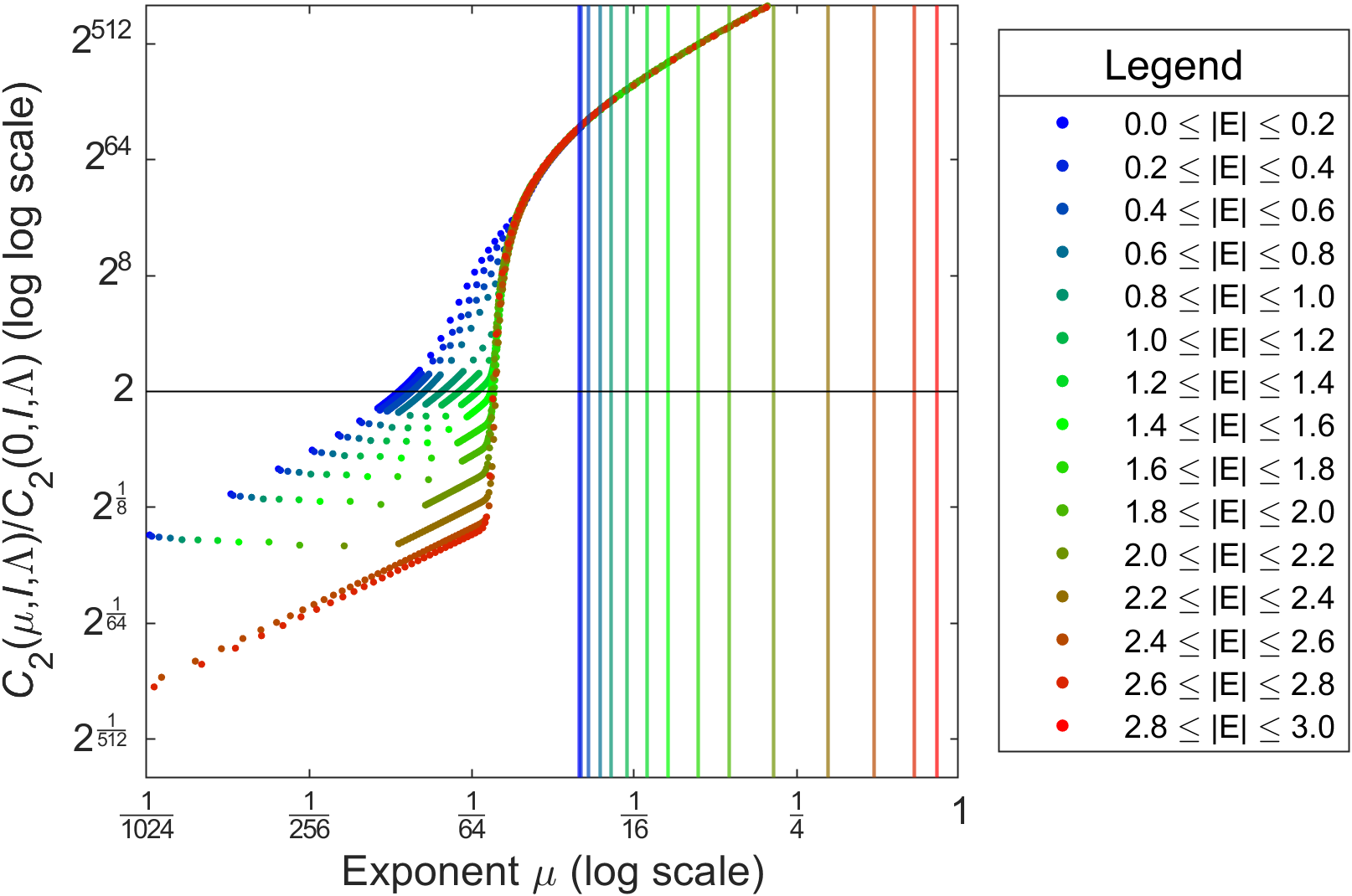
As recalled in §A below, the localization property (A3) is a consequence of an exponentially weighted bound on averaged eigenfunction correlators:

(3.2) $$C_{1}(\nu,I,\Lambda)\ :=\ \frac{1}{\#\Lambda}\sum_{x,y\in\Lambda}e^{\nu|x-y|}{\mathbb{E}}\left(\sum_{E\in I\cap{\mathcal{E}}((H_{\omega})_{\Lambda})}|\varphi_{E}(x)||\varphi_{E}(y)|\right)\ \leq\ A_{\nu}\ ,$$

with $\nu>0$ and $A_{\nu}<\infty$ that may depend on the choice of the energy interval $I$ but are independent of the region $\Lambda$. Because the Lyapunov exponent describes the almost certain tail behavior of eigenfunctions, one is tempted to suppose that $A_{\nu}<\infty$ for $\displaystyle\nu=L(I):=\textstyle{\inf_{E\in I}}L(E)$. However, on closer inspection this seems unlikely. Indeed, for $\nu=L(I)$ we should have $\sup_{\Lambda}C_{1}(\nu,I,\Lambda)=\infty$, since for any sufficiently large finite volume $\Lambda$ a certain fraction of the eigenfunctions will exhibit decay with an exponent smaller than $\nu$, allowing the exponential weight in (3.2) to dominate for large $\Lambda$. Indeed, known proofs of localization yield a correlator bound of the form (3.2) with an exponent $\nu$ that is strictly less than $L(I)$, e.g., $\nu<\frac{1}{2}L(I)$ in [3, Chapter 12]. We are not aware of an estimation in the literature of the exact exponent $\nu_{c}$ at which $C_{1}(\nu_{c},I)$ diverges, nor of a precise estimate of the divergence as $\nu\uparrow\nu_{c}$.

To compute onset lengths, one must choose a particular value of the exponent $\mu$. As shown in §A, the constant $A_{\mathrm{AL}}$ appearing in (A3), and thus in the a priori bound on onset lengths in Prop. 2.1, is bounded by the correlator $C_{1}(2\mu,I,\Lambda)$. In a concrete context, it is important to choose the exponent $\mu$ so that $C_{1}(2\mu,I,\Lambda)$, or some other quantity giving an a priori bound on the onset lengths, is not too large. For the purposes of the numerical investigations reported here, we found it convenient to work with the following $\ell^{2}$, or density-density, correlator:

(3.3) $$C_{2}(\mu,I,\Lambda)\ =\ \frac{1}{\#\Lambda}\sum_{x,y\in\Lambda}e^{2\mu|x-y|}{\mathbb{E}}\left(\sum_{E\in I\cap{\mathcal{E}}((H_{\omega})_{\Lambda})}|\varphi_{E}(x)|^{2}|\varphi_{E}(y)|^{2}\right)\ .$$

Since all eigenfunctions are pointwise bounded by $1$, we have the trivial bound $C_{2}(\mu,I,\Lambda)\leq C_{1}(2\mu,I,\Lambda)$. In the limit $\mu\rightarrow 0$, we have

(3.4) $$C_{2}(0,I,\Lambda)\ =\ \frac{{\mathbb{E}}\left(\#(I\cap{\mathcal{E}}((H_{\omega})_{\Lambda}))\right)}{\#\Lambda}\ ,$$

which is the finite volume integrated density of states on $I$.

(a) On each energy interval with observed eigenvalues (see Fig. 1(b)), the exponent $\mu$ at which $\nicefrac{{C_{2}(\mu,I,\Lambda)}}{{C_{2}(0,I,\Lambda)}}=2$ is shown in blue and the ratio $\nicefrac{{\mu}}{{L(I)}}$ is plotted in red, where $L(I)$ is the minimal Lyapunov exponent on $I$.

(b) Onset length $\ell_{E}$ versus energy $E$ for the eigenfunctions from $240$ samples ($480,000$ eigenfunctions in total). Only $6,313$ (1.3% of the total) eigenfunctions have $\ell_{E}>0$.

Figure 2. Exponents and onset length for eigenfunctions of the 1D Anderson model on an interval of 2000 with disorder $\lambda=1$..

In Fig. 1(b), numerical estimates of the normalized correlators $\nicefrac{{C_{2}(\mu,I,\Lambda)}}{{C_{2}(0,I,\Lambda)}}$ for $(H_{\omega})_{\Lambda}$ with $\lambda=1$ and $\Lambda=[1,2000]$ are shown for 14 energy intervals and various values of $\mu$. These computations were obtained by averaging results from 240 samples of direct diagonalization of $(H_{\omega})_{\Lambda}$. Note that the correlator blows up to extremely large values ($2^{256}\approx 10^{77}$) well before $\mu$ approaches the Lyapunov exponent — observe the $\log\log$ scale on the ordinate of the plot!

(a) $\ell^{\infty}$ norm versus energy for the eigenfunctions from $240$ samples ($480,000$ eigenfunctions in total).

(b) $\ell^{\infty}$ norm versus $\ell_{E}$ for the eigenfunctions from $240$ samples ($480,000$ eigenfunctions in total).

Figure 3. $\ell^{\infty}$ norms versus energy and onset length for eigenfunctions of the 1D Anderson model on an interval of 2000 with disorder $\lambda=1$.

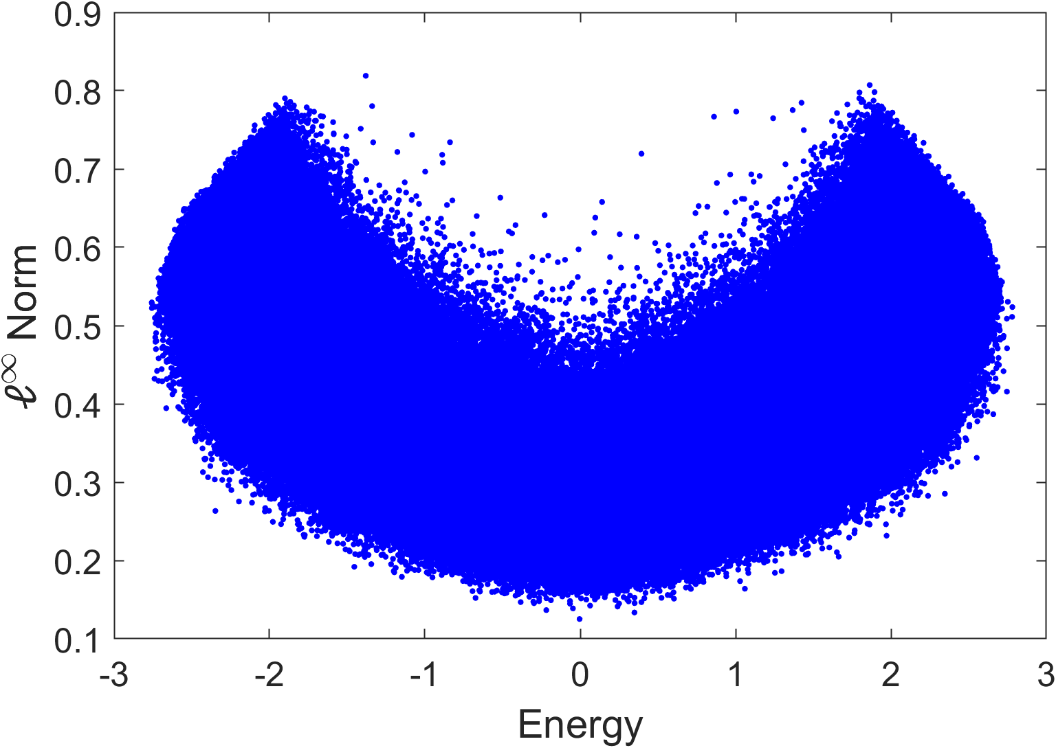
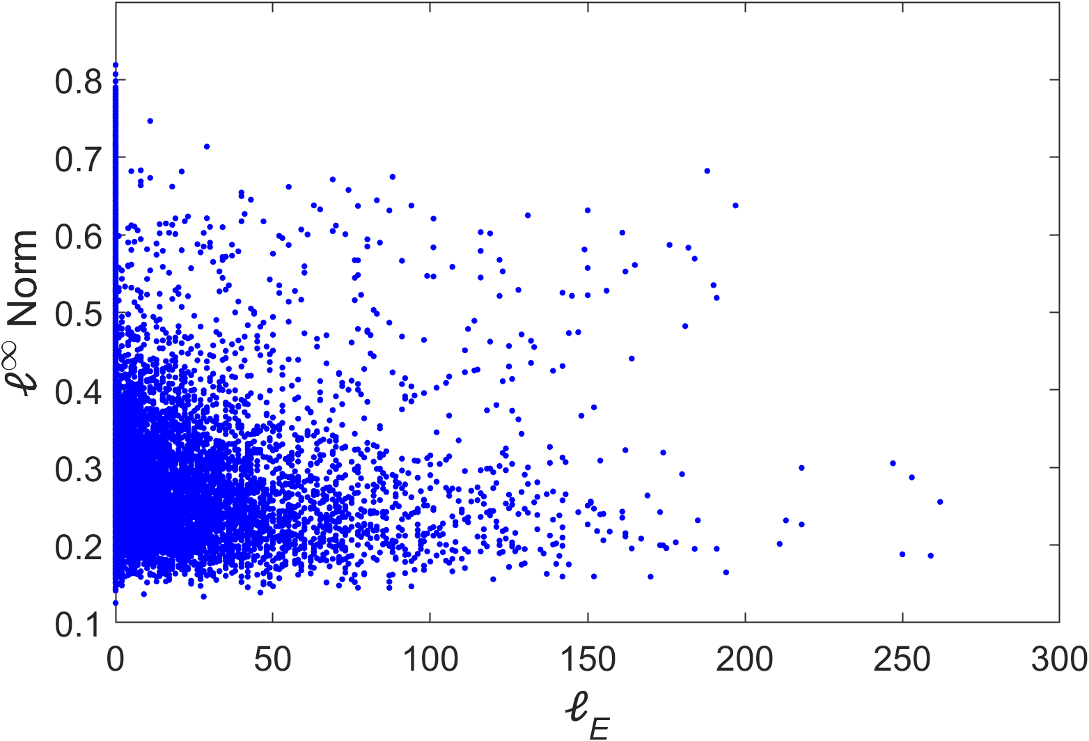
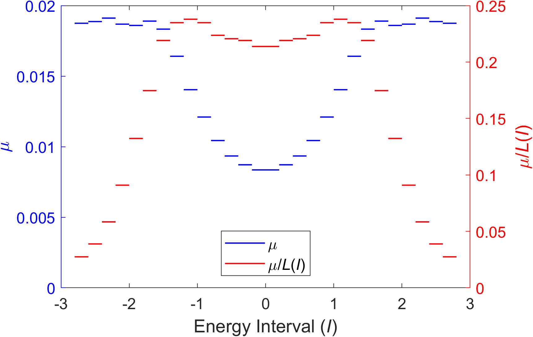
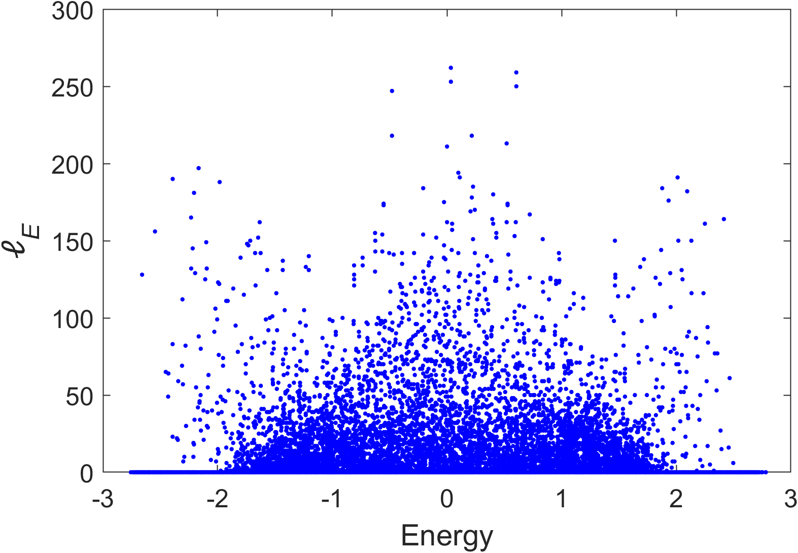
To compute onset lengths for each energy interval, we chose an exponent $\mu=\mu_{I}$ such that the correlator $\nicefrac{{C_{2}(\mu,I,\Lambda)}}{{C_{2}(0,I,\Lambda)}}\approx 2$ (for reference the horizontal cutoff at $2$ is shown in Fig. 1(b)). These exponents are plotted for each of the fourteen energy intervals from $0$ to $2.8$ in Fig. 2(a), along with the ratio $\mu/L(I)$ for each interval. In Fig. 2(b), the onset length $\ell_{E}$ for each of the $480,000$ eigenfunctions is plotted against the corresponding eigenvalue. Only $6,313$ eigenfunctions (1.3% of the total) were found to have positive onset length, and the maximum onset length observed was 262. For comparison, the $\ell^{\infty}$ norms of the eigenfunctions are plotted in Fig. 3, versus energy and versus onset length. Within the range of attained $\ell^{\infty}$ norms, there is little correlation with the onset length.

It is natural to wonder whether the observation of onset lengths as large as 262 is consistent with the estimation that these numbers should be “of order $\log\#\Lambda\approx 7.6$.” However, the correlator bound $C_{2}(\mu,I,\Lambda)\leq 2*C_{2}(0,I,\lambda)$ provides an a priori bound on localization lengths that is consistent with this observation, as follows. From the Markov inequality, we have with probability at least $1-\epsilon$ that

$$\frac{1}{\#\Lambda}\sum_{x,y\in\Lambda}e^{2\mu|x-y|}\sum_{E\in I\cap{\mathcal{E}}((H_{\omega})_{\Lambda})}|\varphi_{E}(x)|^{2}|\varphi_{E}(y)|^{2}\ \leq\ \frac{2*C_{2}(0,I,\lambda)}{\epsilon}.$$

Fixing a particular energy $E$ and taking $y=x_{E}$, we see that each eigenfunction satisfies

$$\sum_{x}e^{2\mu|x-x_{E}|}|\varphi_{E}(x)|^{2}\ \leq\ \frac{2*C_{2}(0,I,\Lambda)\#\Lambda}{\epsilon\|\varphi_{E}\|_{\infty}^{2}}\ .$$

Following the proof of Prop. 2.1, we find that

$$\ell_{E}\ \leq\ \frac{1}{2\mu}(\log 2C_{2}(0,I,\Lambda)+\log\#\Lambda-\log 3\epsilon-2\log\|\varphi_{E}\|_{\infty})+1.$$

In the current context, we take $\epsilon=1/240$, as this is the smallest probability we can resolve with 240 samples. The key point is that we expect onset lengths to be no larger than $\frac{1}{2\mu}(\log\#\Lambda-\log 3\epsilon)$, where we have neglected the relatively smaller terms coming from the $\|\varphi_{E}\|_{\infty}$ norm and $C_{2}(0,I,\Lambda)$. For $\#\Lambda=2000$, $\epsilon=1/240$, and $\mu\approx 0.01$, we obtain a rough bound of order $600$. So we should not be surprised to see onset lengths of the size seen here.

(a) Cumulative distribution of onset lengths for $240$ samples with $\lambda=1$ on an interval of length $2000$.

(b) Cumulative distribution of onset lengths for $390$ samples with $\lambda=2$, $4$, $8$ and $16$ on an interval of length $1000$.

Figure 4. Cumulative distribution of onset lengths for eigenfunctions of the 1D Anderson model.

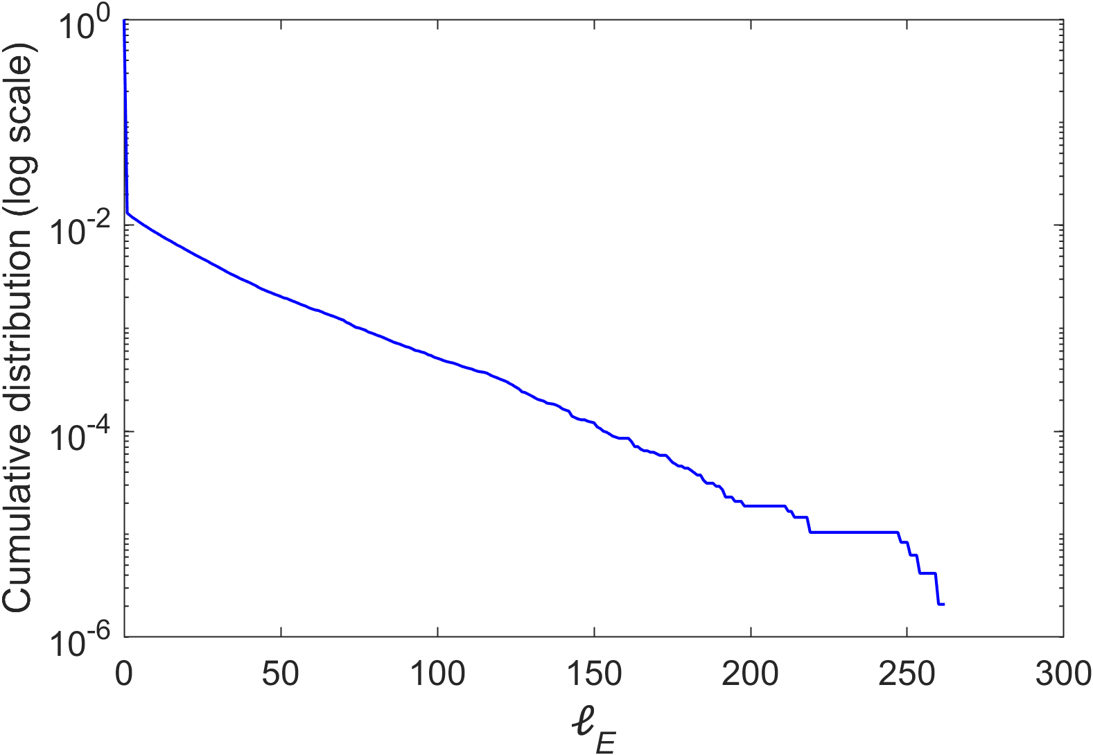
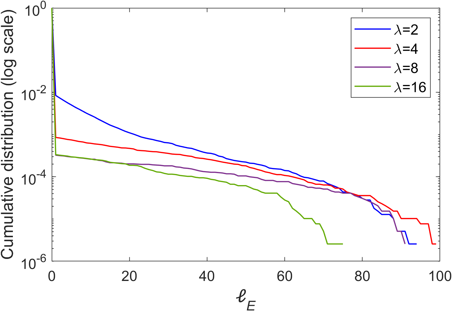
The cumulative distributions of onset lengths for various disorder strengths are shown in Fig. 4. On the left, we have plotted the results for the $\lambda=1$ and $\Lambda=[1,2000]$. On the right, one finds results for $\lambda=2$, $4$, $8$ and $16$ on the interval $[1,1000]$, computed by the same methods indicated above. Notably, for each disorder strength after a sharp drop off from $\ell_{E}=0$ to $\ell_{E}=1$, the cumulative distribution exhibits exponential decay over a range of lengths before dropping off at the maximum attained onset length within the geometry and number of simulations.

Figure 5. Three digenfunctions for the 1D Anderson model on $\Lambda=[1,2000]$ with $\lambda=1$.

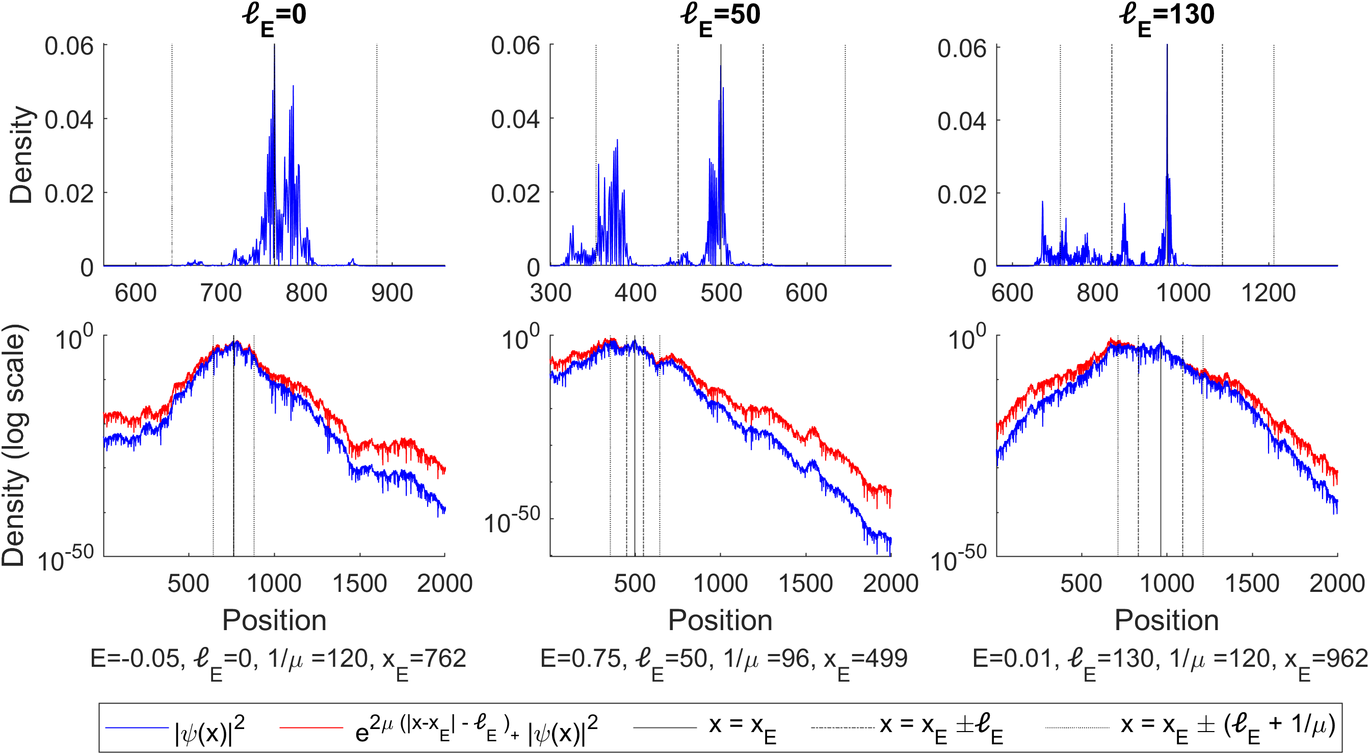
As the proof of Thm. 2.1 will show, an eigenfunction can have a large onset length due to a large deviation of the random environment in a neighborhood of the localization center. As such, although all eigenfunctions share the same exponential decay in their tails, the behavior of an eigenfunction over the localization volume $x_{E}\pm\ell_{E}$ is, by definition, atypical. To paraphrase Tolstoy, all eigenfunctions with small onset length are alike, each eigenfunction with large onset length is extended in its own way. To illustrate the variety of behaviors possible within the localization volume, we have have plotted the density $|\psi_{E}(x)|^{2}$ for three different eigenfunctions in Fig. 5. In the upper plots, the density of each eigenfunction is shown in a neighborhood of the localization center. In the lower plots, the logarithm of the density and of the exponentially weighted density $e^{2\mu(|x-x_{E}|-\ell_{E})_{+}}|\psi_{E}(x)|^{2}$ are shown for the entire chain $[1,2000]$. The first eigenfunction, with onset length $\ell_{E}=0$, has the majority of its mass within one localization length ($\nicefrac{{1}}{{\mu}}$) of the localization center. The second eigenfunction, with onset length $\ell_{E}=50$, shows two distinct peaks at roughly distance $\ell_{E}+\nicefrac{{1}}{{\mu}}$ from each other. This sort of resonant superposition of two or more localization centers is one mechanism for the development of a substantial onset length. Although rare, such eigenfunctions will appear with positive frequency in large systems. Finally, the third eigenfunction, with onset length $\ell_{E}=130$, is extended over an interval of size roughly $\ell_{E}+1/\mu$. On mechanism for the occurrence of such eigenfunctions is for the potential over the interval $[x_{E}-\ell_{E},x_{E}+\ell_{E}]$ to closely mimic a potential having extended states (e.g., a periodic potential) or a long localization length at energy $E$. This is the behavior one finds for the eigenfunctions from the Lifshitz tail regime (see Thm. 2.2), although this particular eigenfunction comes from the center of the band ($E=0.01$).

4. The proofs of Theorem 2.1 and Theorem 2.3

We now turn to the proof of Theorem 2.1 for the discrete Anderson model. Let $\alpha\in\frac{1}{2}{\mathbb{N}}$, $\alpha\geq 1$; this parameter is arbitrary but will be fixed throughout our analysis. Given a lattice cube $Q=\Lambda_{\ell}(x_{0})$ of center $x_{0}\in{\mathbb{Z}}^{d}$ and side length $\ell\in{\mathbb{N}}$, we let $\widetilde{Q}:=\Lambda_{(2\alpha+1)\ell}(x_{0})$ denote the expanded cube with the same center but side length $(2\alpha+1)\ell$ (see Figure 6). Our first result shows how to approximate an eigenfunction $\varphi_{E}$ on a region $\Omega$ with localization center $x_{E}\in Q$ by an eigenfunction $\psi_{E^{\prime}}\in\ell^{2}(\widetilde{Q})$ of the Hamiltonian $(H_{\omega})_{\widetilde{Q}}$ on the expanded cube.

Lemma 4.1.

Let $\Omega\subset{\mathbb{Z}}^{d}$ be a region and let $S=\Omega\cap Q$, where $Q=\Lambda_{\ell}(x_{0})$ is a cube of side length $\ell\geq 2$ such that $Q\cap\Omega\neq\emptyset$. Let $\widetilde{S}=\widetilde{Q}\cap\Omega$, let $0<\delta<1$ and fix a disorder configuration $\omega$ such that

(4.1) $$\max_{E\in\sigma\left((H_{\omega})_{\widetilde{S}}\right)}{\rm tr}\,\mathbf{1}_{E+[-\delta,\delta]}[(H_{\omega})_{\widetilde{S}}]\ \leq\ 1\ .$$

If there is an eigenvalue $E\in{\mathcal{E}}((H_{\omega})_{\Omega})$ of $(H_{\omega})_{\Omega}$ with normalized eigenvector $\varphi_{E}$ such that $x_{E}\in S$ and

(4.2) $$M\ :=\ \left(\sum_{x}e^{2\mu|x-x_{E}|}|\varphi_{E}(x)|^{2}\right)^{\frac{1}{2}}\ \leq\frac{\delta e^{\alpha\mu\ell}}{2\sqrt{d}}\ ,$$

then there exists a unique eigenvalue $E^{\prime}\in{\mathcal{E}}((H_{\omega})_{\widetilde{S}})$ of $(H_{\omega})_{\widetilde{S}}$ with normalized eigenvector $\psi_{E^{\prime}}$ such that

(4.3) $$|E-E^{\prime}|\ \leq\ 2\sqrt{d}Me^{-\alpha\mu\ell}\ ,$$

and

(4.4) $$\left\|\mathbf{1}_{\widetilde{S}}\varphi_{E}-\psi_{E^{\prime}}\right\|_{\ell^{2}(\widetilde{S})}\ \leq\ 3\sqrt{d}\frac{M}{\delta}e^{-\alpha\mu\ell}\ .$$

Figure 6. The setup of Lemma 4.1, showing a cube $Q$ and its expansion $\widetilde{Q}$ intersected with a region $\Omega$.

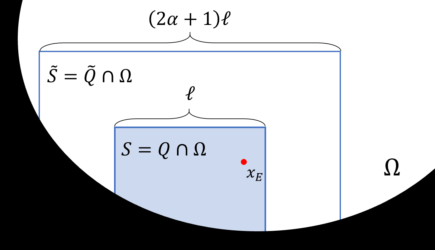
Proof.

Since $x_{E}\in S$, we have

(4.5) $$\|\varphi_{E}\|_{\ell^{2}(\Omega\setminus\widetilde{S})}\ =\ \left(\sum_{x\in\Omega\setminus\widetilde{S}}|\phi_{E}(x)|^{2}\right)^{\frac{1}{2}}\ \leq\ \ e^{-\alpha\mu\ell}\left(\sum_{x\in\Omega}e^{2\mu|x-x_{E}|}|\phi_{E}(x)|^{2}\right)^{\frac{1}{2}}\ =\ Me^{-\alpha\mu\ell}\ .$$

Thus by (4.2),

(4.6) $$\|\mathbf{1}_{\widetilde{S}}\varphi_{E}\|_{\ell^{2}(\widetilde{S})}\ \geq\ 1-Me^{-\alpha\mu\ell}\ \geq\ 1-\frac{\delta}{2\sqrt{d}}\ >\ \frac{1}{2}\ .$$

Since $(H_{\omega})_{\widetilde{S}}$ is the restriction of $(H_{\omega})_{\Omega}$ to $\widetilde{S}$ and $\varphi_{E}$ is an eigenvector of $(H_{\omega})_{\Omega}$, we see that

$$\left[(H_{\omega})_{\widetilde{S}}-E\right]\mathbf{1}_{\widetilde{S}}\varphi_{E}(x)=\begin{cases}0&\text{if }x\in\widetilde{S}\text{ and }{\rm dist}\,(x,\Omega\setminus\widetilde{S})\geq 2\ ,\text{ and}\\ {\displaystyle\sum_{\begin{subarray}{c}y\in\Omega\setminus\widetilde{S}\\ |y-x|=1\end{subarray}}}\varphi_{E}(y)&\text{if }x\in\widetilde{S}\text{ and }{\rm dist}\,(x,\Omega\setminus\widetilde{S})=1\ .\end{cases}$$

Because each $x\in\widetilde{S}$ has at most $d$ neighbors in $\Omega\setminus\widetilde{S}$,

(4.7) $$\left\|\left[(H_{\omega})_{\widetilde{S}}-E\right]\mathbf{1}_{\widetilde{S}}\varphi_{E}\right\|\ \leq\ \left(d\sum_{y\in\Omega\setminus\widetilde{S}}|\varphi_{E}(y)|^{2}\right)^{\frac{1}{2}}\ \leq\ \sqrt{d}Me^{-\alpha\mu\ell}.$$

Since $(H_{\omega})_{\widetilde{S}}$ is self adjoint, (4.7) and (4.6) together imply that one of the eigenvalues of $(H_{\omega})_{\widetilde{S}}$, call it $E^{\prime}$, satisfies (4.3).

Let $\psi_{E^{\prime}}$ be the normalized eigenvector associated to $E^{\prime}$; we fix its phase by requiring $\langle\psi_{E^{\prime}}\,,\,\mathbf{1}_{\widetilde{S}}\varphi_{E}\rangle>0$. To estimate $\left\|\mathbf{1}_{\widetilde{S}}\varphi_{E}-\psi_{E^{\prime}}\right\|_{\ell^{2}(\widetilde{S})}$, note that

(4.8) $$\left\|\mathbf{1}_{\widetilde{S}}\varphi_{E}-\psi_{E^{\prime}}\right\|_{\ell^{2}(\widetilde{S})}\ \leq\ \|\mathbf{1}_{\widetilde{S}}\varphi_{E}-\langle\psi_{E^{\prime}}\,,\,\mathbf{1}_{\widetilde{S}}\varphi_{E}\rangle\psi_{E^{\prime}}\|_{\ell^{2}(\widetilde{S})}+1-\langle\psi_{E^{\prime}}\,,\,\mathbf{1}_{\widetilde{S}}\varphi_{E}\rangle\\ \leq\ 2\|\mathbf{1}_{\widetilde{S}}\varphi_{E}-\langle\psi_{E^{\prime}}\ ,\ \mathbf{1}_{\widetilde{S}}\varphi_{E}\rangle\psi_{E^{\prime}}\|_{\ell^{2}(\widetilde{S})}+\|\varphi_{E}\|_{\ell^{2}(\Omega\setminus\widetilde{S})},$$

since $\langle\psi_{E^{\prime}}\,,\,\mathbf{1}_{\widetilde{S}}\varphi_{E}\rangle\geq\|\mathbf{1}_{\widetilde{S}}\varphi_{E}\|_{\ell^{2}(\widetilde{S})}-\|\mathbf{1}_{\widetilde{S}}\varphi_{E}-\langle\psi_{E^{\prime}}\,,\,\mathbf{1}_{\widetilde{S}}\varphi_{E}\rangle\psi_{E^{\prime}}\|_{\ell^{2}(\widetilde{S})}$. By (4.1), $E^{\prime}$ is non-degenerate and at least distance $2\delta$ from every other eigenvalue of $(H_{\omega})_{\widetilde{S}}$. Thus it follows from (4.7) and (4.3) that

(4.9) $$\|\mathbf{1}_{\widetilde{S}}\varphi_{E}-\langle\psi_{E^{\prime}}\,,\,\mathbf{1}_{\widetilde{S}}\varphi_{E}\rangle\psi_{E^{\prime}}\|\ \leq\ \frac{\sqrt{d}Me^{-\alpha\mu\ell}}{2\delta-2\sqrt{d}Me^{-\alpha\mu\ell}}\ \leq\ \ \sqrt{d}\frac{M}{\delta}e^{-\alpha\mu\ell}\ ,$$

where we have used (4.2) in the last step. Equation (4.4) follows from (4.8), (4.9), and (4.5). ∎

For a given sufficiently large length scale $L$ and a region $\Omega$ containing a cube $\Lambda_{L}(x_{0})$ of size $L$, we will consider partitions of $\Omega$ into smaller cubes along a decreasing sequence of scales, depending on $L$:

(4.10) $$L_{1}=\lfloor\beta\log L\rfloor\quad\text{and}\quad L_{n}=\lfloor\tfrac{1}{4}L_{n-1}\rfloor\quad\text{for }2\leq n\leq n_{\mathrm{fin}}\ .$$

Here $\beta>0$ is a constant to be chosen below and $n_{\mathrm{fin}}=n_{\mathrm{fin}}(L)$ is the largest value of $n$ such that $L_{n}\geq L_{\mathrm{fin}}$, where $L_{\mathrm{fin}}>1$ is an (integer) length scale which we take sufficiently large, but fixed independent of $\Omega$ and $L$. In particular, we require that $L_{\mathrm{fin}}\geq e$ and $L_{\mathrm{fin}}>\beta\log L_{\mathrm{fin}}$, so that $L_{1}=\beta\log L<L$ for $L>L_{\mathrm{fin}}$. Without loss of generality, we suppose that $L\geq\exp(\nicefrac{{L_{\mathrm{fin}}}}{{\beta}})$ so that $L>L_{1}\geq L_{\mathrm{fin}}$ and $n_{\mathrm{fin}}\geq 1$. Note that $L_{\mathrm{fin}}\leq L_{n_{\mathrm{fin}}}<4L_{\mathrm{fin}}$ and

(4.11) $$(\tfrac{1}{4})^{n-1}\beta\log L-\frac{4}{3}\ <\ L_{n}\ \leq\ (\tfrac{1}{4})^{n-1}\beta\log L.$$

As a result, we have the estimate

(4.12) $$\frac{1}{\log 4}\log\log L+\frac{\log\beta-\log(L_{\mathrm{fin}}+\frac{1}{3})}{\log 4}\ <n_{\mathrm{fin}}(L)\ \leq\ \frac{1}{\log 4}\log\log L+\frac{\log\beta-\log L_{\mathrm{fin}}}{\log 4}+1\ .$$

In particular $n_{\mathrm{fin}}(L)=O(\log\log L)$ as $L\rightarrow\infty$. For future reference we note the following

Proposition 4.1.

For every $\nu>0$ and $1\leq n\leq n_{\mathrm{fin}}$,

(4.13) $$e^{-\nu L_{n}}\ <\ \sum_{j=1}^{n}e^{-\nu L_{j}}\ <\ \frac{e^{-\nu L_{n}}}{1-e^{-\nu L_{n}}}\ <\ \left(1+\frac{1}{e^{\nu L_{\mathrm{fin}}}-1}\right)e^{-\nu L_{n}}\ .$$

Proof.

Since $L_{j}\geq 4L_{j+1}$, we see that $L_{j}\geq 4^{n-j}L_{n}$ for $1\leq j\leq n$. Thus

$$\sum_{j=1}^{n}e^{-\nu L_{j}}\ \leq\ \sum_{j=0}^{n-1}e^{-\nu 4^{j}L_{n}}\ <\ \sum_{j=0}^{\infty}e^{-\nu 4^{j}L_{n}}\ <\ e^{-\nu L_{n}}\sum_{j=0}^{\infty}e^{-3j\nu L_{n}}\ <\ e^{-\nu L_{n}}\sum_{j=0}^{\infty}e^{-j\nu L_{n}}\ ,$$

from which the upper bounds follow. The lower bound is clear. ∎

We now fix a region $\Omega\subset{\mathbb{Z}}^{d}$ and a length scale $L$. For each generation $1\leq n\leq n_{\mathrm{fin}}$, let

$$\mathcal{G}^{n}\ :=\ \left\{\Lambda_{L_{n}}(L_{n}\mathbf{k})\cap\Omega\ :\ \mathbf{k}\in{\mathbb{Z}}^{d}\text{ and }\Lambda_{L_{n}}(L_{n}\mathbf{k})\cap\Omega\neq\emptyset\right\}\ ,$$

Figure 7. Cubes of generation $n$ and $n+1$. Note that the neighboring cubes $Q_{1}^{n}$ and $Q_{2}^{n}$ do not overlap, but the extended cubes $\widetilde{Q}_{1}^{n}$ and $\widetilde{Q}_{2}^{n}$ do.

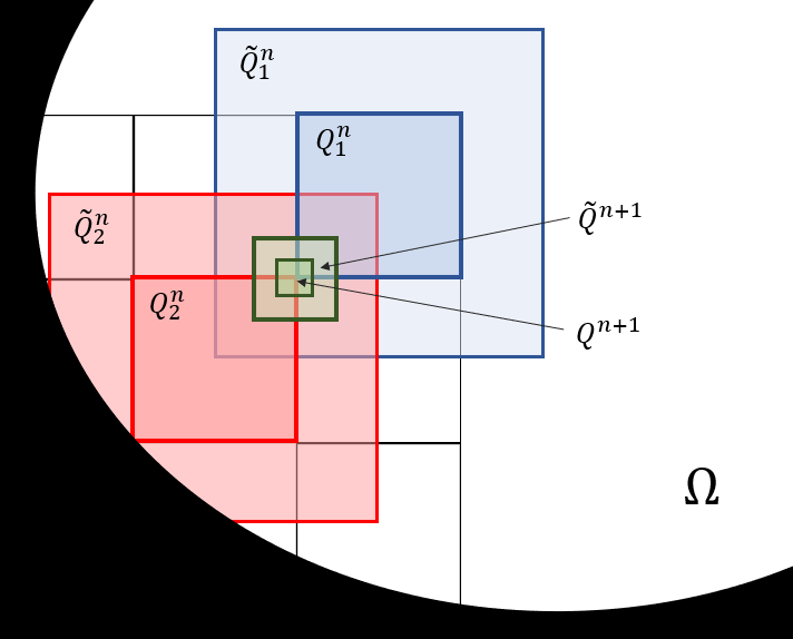
which is the set of cubes centered on $L_{n}{\mathbb{Z}}^{d}$ of side length $L_{n}$ which overlap $\Omega$ (see Figure 7). (We shall refer to the elements of $\mathcal{G}^{n}$ as “cubes,” although those that intersect the boundary of $\Omega$ consist only of a portion of a cube.) Note that a cube $Q\in{\mathcal{G}}^{n}$ and its expansion $\widetilde{Q}$ have volumes

(4.14) $$\hskip-199.16928pt\#Q\ \leq\ L_{n}^{d}\quad\text{ and }\quad\#\widetilde{Q}\ \leq\ (2\alpha+1)^{d}L_{n}^{d}\ ,$$

with equality unless the cube $Q$ or its expansion $\widetilde{Q}$ intersect the boundary of $\Omega$. With these definitions, we see that

1. If $Q,Q^{\prime}\in{\mathcal{G}}^{n}$ and $Q\neq Q^{\prime}$, then $Q\cap Q^{\prime}=\emptyset$.

2. $\displaystyle\Omega\ =\ \bigcup_{Q\in{\mathcal{G}}^{n}}Q$.

Given a region $S\subset\Omega$, let

$$\hskip-199.16928pt{\mathcal{G}}^{n}(S)\ :=\ \left\{Q\in{\mathcal{G}}^{n}\ :\ Q\cap S\neq\emptyset\right\}.$$

We note that if $S=\Lambda_{L}(x)\subset\Omega$ is a cube then we have the bounds:

(4.15) $$\hskip-227.62204pt\left(\frac{L}{L_{n}}\right)^{d}\ \leq\ \#\mathcal{G}^{n}(\Lambda_{L}(x))\ \leq\ \left(\frac{L}{L_{n}}+2\right)^{d}$$

Given a cube $Q\in{\mathcal{G}}^{n}$ of generation $n$ and a realization $\omega$ of the random potential, let

$$M_{\omega}(Q)\ =\ \max_{E\in\Sigma(\widetilde{Q})}\max_{y\in\mathcal{C}(\varphi_{E})}\left(\sum_{x\in\widetilde{Q}}|\varphi_{E}(x)|^{2}e^{2\mu|x-y|}\right)^{\frac{1}{2}}\ ,$$

where $\Sigma(\widetilde{Q})={\mathcal{E}}((H_{\omega})_{\widetilde{Q}})\cap I_{\text{AL}}$ and $\varphi_{E}$ is the $\ell^{2}$-normalized eigenvector of of $(H_{\omega})_{\widetilde{Q}}$ corresponding to the eigenvalue $E\in\Sigma(\widetilde{Q})$. For $n\geq 1$, we say that $Q\in{\mathcal{G}}^{n}$ is $\epsilon$-good (for a given realization $\omega$) if the following conditions are satisfied:

1. $M_{\omega}(Q)\leq e^{\epsilon\lfloor\frac{1}{4}L_{n}\rfloor}$;

2. Eq. (4.1) holds for $\widetilde{Q}$ with $\delta=e^{-\frac{\epsilon}{2}L_{n}}$, i.e.,

   (4.16) $$\max_{E\in\sigma\left((H_{\omega})_{\widetilde{Q}}\right)\cap I_{\mathrm{AL}}}{\rm tr}\,\mathbf{1}_{E+[-e^{-\frac{\epsilon}{2}L_{n}},e^{-\frac{\epsilon}{2}L_{n}}]}[(H_{\omega})_{\widetilde{Q}}]\ \leq\ 1.$$

Note that the exponent in (1) involves $\lfloor\frac{1}{4}L_{n}\rfloor=L_{n+1}$, which is the next length scale. By a bound similar to (4.5), if $Q\in{\mathcal{G}}^{n}$ is an $\epsilon$-good cube and $\ell>0$, then

(4.17) $$\|\mathbf{1}_{\{x:|x-x_{E}|\geq\ell\}}\varphi_{E}\|_{\ell^{2}(\widetilde{Q})}\ \leq\ e^{-\mu\ell+\epsilon\lfloor\frac{1}{4}L_{n}\rfloor}$$

for any $E\in\Sigma(\widetilde{Q})$ and $x_{E}\in\mathcal{C}(\varphi_{E})$. The cube $\widetilde{Q}$ is called $\epsilon$-bad (for a given realization $\omega$) if it is not $\epsilon$-good.

By iterating Lemma 4.1, we can obtain the following:

Lemma 4.2.

Let $0<\epsilon\leq\frac{\alpha}{8}\mu$, let $p>0$, and let $\beta\geq\frac{4}{\alpha\mu}(p+d)$. Let $[a,b]\subset I_{\mathrm{AL}}$ be a compact interval with $r={\rm dist}\,([a,b],I_{\mathrm{AL}}^{c})>0$, let $L_{\mathrm{fin}}$ be such that $L_{\mathrm{fin}}>\beta\log L_{\mathrm{fin}}$,

(4.18a) $$L_{\mathrm{fin}}\ \geq\ \max\left(4,\ \frac{8}{5\alpha\mu}\log 2,\ \frac{8}{7\alpha\mu}\log\tfrac{4\sqrt{d}}{r}\right)\,$$

and

(4.18b) $$\sup_{L\geq\frac{1}{32}L_{\mathrm{fin}}}(4L+1)^{\frac{d}{2}}e^{-\mu L}\ \leq\ \frac{1}{8\sqrt{d}},$$

and let $L\geq\exp(\nicefrac{{L_{\mathrm{fin}}}}{{\beta}})$. If $\Omega\subset{\mathbb{Z}}^{d}$ is a region and $\Lambda_{L}(x_{0})\cap\Omega\neq\emptyset$ for some $x_{0}$, then, with probability at least $1-(e^{\frac{\alpha\mu}{8}}A_{\mathrm{AL}})^{2}L^{-p}$, to each eigenvalue

$$E\ \in\ \Sigma(\Lambda_{L}(x_{0}))\ :=\ \{E\in{\mathcal{E}}((H_{\omega})_{\Omega})\cap[a,b]\ :\ \mathcal{C}(\varphi_{E})\cap\Lambda_{L}(x_{0})\neq\emptyset\}$$

are associated finite sequences $(Q_{E}^{j})_{j=1}^{m_{E}}$, $(\psi_{E}^{j})_{j=0}^{m_{E}}$, and $(\lambda_{E}^{j})_{j=0}^{m_{E}}$ where:

1. $\psi_{E}^{0}=\varphi_{E}$ and $\lambda_{E}^{0}=E$;

2. if $m_{E}\geq 1$, then, for $j=1,\ldots,m_{E}$,

   1. the cube $Q_{E}^{j}$ is $\epsilon$-good and $\mathcal{C}(\psi_{E}^{j-1})\cap Q_{E}^{j}\neq\emptyset$;

   2. if $j\geq 2$, then $\widetilde{Q}_{E}^{j}\subset\widetilde{Q}_{E}^{j-1}$;

   3. $\psi_{E}^{j}$ is an eigenfunction of $(H_{\omega})_{\widetilde{Q}_{E}^{j}}$ with eigenvalue $\lambda_{E}^{j}$;

   4. we have

      (4.19) $$|\lambda_{E}^{j}-\lambda_{E}^{j-1}|\ \leq\ 2\sqrt{d}\,e^{-(\alpha\mu-\epsilon)L_{j}},$$

      and

      (4.20) $$\|\psi_{E}^{j}-\mathbf{1}_{\widetilde{Q}_{E}^{j}}\psi_{E}^{j-1}\|_{\ell^{2}(\widetilde{Q}_{E}^{j})}\ \leq\ 3\sqrt{d}\,e^{-(\alpha\mu-3\epsilon)L_{j}}\ ;$$

3. either $m_{E}=n_{\mathrm{fin}}$ or every cube $Q\in{\mathcal{G}}^{m_{E}+1}$ with $Q\cap\mathcal{C}(\psi_{E}^{j})\neq\emptyset$ and $\widetilde{Q}\subset\widetilde{Q}_{E}^{m_{E}}$ is $\epsilon$-bad.

Furthermore, taking $Q_{E}^{0}=\widetilde{Q}_{E}^{0}=\Omega$ and $L_{0}=L$, we have

1. given integers $0\leq j_{E}\leq m_{E}$ for each $E\in\Sigma(\Lambda_{L}(x_{0}))$, the map $E\mapsto(Q_{j_{E}},\psi_{E}^{j_{E}},\lambda_{j_{E}})$ is one-to-one,

2. for any $y\in\mathcal{C}(\psi_{E}^{m_{E}})$,

   (4.21) $$\mathcal{C}(\psi_{E}^{j})\subset\{x:|x-y|<\frac{\alpha}{16}L_{m_{E}}\}\subset\widetilde{Q}_{E}^{m_{E}}\ ,$$

   for each $j=0,\ldots,m_{E}$, and

3. if $(1+\alpha)\nu<\alpha\mu-4\epsilon$, then

   (4.22) $$\left(\sum_{x\in\widetilde{Q}_{E}^{j}}e^{2\nu|x-y|}|\psi_{E}^{j}(x)|^{2}\right)^{\frac{1}{2}}\ \leq\ \left(1+\frac{1+3\sqrt{d}}{e^{\epsilon L_{m_{E}}}-1}\right)e^{(\frac{\alpha}{8}+\frac{\epsilon}{4})\nu L_{m_{E}}}$$

   for any $y\in\mathcal{C}(\psi_{E}^{j})$.

Remark 4.1.

1) Since $L_{\mathrm{fin}}\geq\frac{8}{5\alpha\mu}\log 2$, Proposition 4.1 implies that

(4.23) $$\sum_{j=1}^{n}e^{-\nu L_{j}}\ <2e^{-\nu L_{n}}\ ,$$

whenever $\nu>\frac{5\alpha}{8}\mu$. 2) Using eqs. (4.19) and (4.23), we see that, for $j=1,\ldots,m_{E}$,

(4.24) $$|\lambda_{E}^{j}-E|\ \leq\ \sum_{k=1}^{j}|\lambda_{E}^{k}-\lambda_{E}^{k-1}|\ \leq\ 4\sqrt{d}e^{-\frac{7\alpha}{8}\mu L_{j}}\ <\ r\ ,$$

since $L_{j}\geq L_{\mathrm{fin}}>\frac{8}{7\mu}\log\tfrac{4\sqrt{d}}{r}$. Thus each eigenvalue is in the localization regime, $\lambda_{E}^{j}\in I_{\mathrm{AL}}$.

Proof.

Let $\Lambda=\Lambda_{L}(x_{0})$ and $\Sigma=\Sigma(\Lambda_{L}(x_{0})).$ By (A3), with probability at least $1-A_{\mathrm{AL}}^{2}e^{\frac{\alpha\mu}{4}}L^{-p}$, we have

(4.25) $$\max_{E\in\Sigma}\max_{y\in\mathcal{C}(\varphi_{E})\cap\Lambda}\left(\sum_{x\in\Omega}|\varphi_{E}(x)|^{2}e^{2\mu|x-y|}\right)^{\frac{1}{2}}\ \leq\ L^{\frac{d+p}{2}}e^{-\frac{\alpha}{8}\mu}\ \leq\ e^{\frac{\alpha}{8}\mu L_{1}}.$$

On the event that eq. (4.25) holds, for each $E\in\Sigma$ we will construct sequences $(Q_{E}^{j})_{j=1}^{m_{E}}$ ,$(\psi_{E}^{j})_{j=0}^{m_{E}}$, $(\lambda_{E}^{j})_{j=0}^{m_{E}}$ satisfying (1)-(4) as well as localization centers $x_{E}^{j}\in\mathcal{C}(\psi_{E}^{j})$, for $j=0,\ldots,m_{E}$, such that $x_{E}^{j}\in Q_{E}^{j+1}$ and

(4.26) $$\mathcal{C}(\psi_{E}^{j+1})\ \subset\ \left\{x:|x-x_{E}^{j}|<\tfrac{\alpha}{4}L_{j+1}\right\}\ ,$$

for $j=0,\ldots,m_{E}-1$.

Fix $E\in\Sigma$ and let $\psi_{E}^{0}=\varphi_{E}$, $\lambda_{E}^{0}=E$. For ease of notation, we take $Q_{E}^{0}=\widetilde{Q}_{E}^{0}=\Omega$. We define the remainder of the sequence recursively. Let $n\geq 0$ and suppose we have already found $(Q_{E}^{j})_{j=0}^{n}$ ,$(\psi_{E}^{j})_{j=0}^{n}$, $(\lambda_{E}^{j})_{j=0}^{n}$ and $(x_{E}^{j})_{j=0}^{n-1}$ with the desired properties. We note that

(4.27) $$M_{n}\ :=\ \left(\sum_{x\in\widetilde{Q}_{E}^{n}}|\psi_{E}^{n}(x)|^{2}e^{2\mu|x-x_{E}^{n}|}\right)^{\frac{1}{2}}\ \leq\ e^{\frac{\alpha}{8}\mu L_{n+1}}\ ;$$

for $n=0$ this follows from (4.25), while, for $n\geq 1$, this holds since $Q_{E}^{n}$ is $\epsilon$-good and $\epsilon\leq\frac{\alpha}{8}\mu$. If $n=n_{\mathrm{fin}}$ or every cube $Q\in{\mathcal{G}}^{n+1}$ with $\mathcal{C}(\psi_{E}^{n})\cap Q\neq\emptyset$ is $\epsilon$-bad, then we choose $x_{E}^{n}$ to be an arbitrary element of $\mathcal{C}(\psi_{E}^{n})$, set $m_{E}=n$, and there is nothing further to show. Otherwise, pick an $\epsilon$-good cube $Q_{E}^{n+1}\in{\mathcal{G}}^{n+1}$ with $Q_{E}^{n+1}\cap\mathcal{C}(\psi_{E}^{n})\neq\emptyset$ and pick $x_{E}^{n}\in Q_{E}^{n+1}\cap\mathcal{C}(\psi_{E}^{n})$. Since $Q_{E}^{n+1}$ is $\epsilon$-good, eq. (4.1) holds with $\delta=e^{-\epsilon L_{n+1}}$. Furthermore, eq. (4.2) follows from eqs. (4.27), since

$$M_{n}\ \leq\ e^{\frac{\alpha}{8}\mu L_{n+1}}\ \leq\ \frac{e^{\frac{5\alpha}{8}\mu L_{n+1}}}{8\sqrt{d}(\frac{5\alpha}{2}L_{n+1})^{\nicefrac{{d}}{{2}}}}\delta e^{\frac{3\alpha}{8}\mu L_{n+1}}\ \leq\ \frac{\delta e^{\alpha\mu L_{n+1}}}{8\sqrt{5}}\ <\ \frac{\delta e^{\alpha\mu L_{n+1}}}{2\sqrt{d}}\ ,$$

where we have used (4.18) and the fact that $\alpha\geq\frac{1}{2}$. Hence by Lemma 4.1, there is an eigenfunction $\psi_{E}^{n+1}$ on $\widetilde{Q}_{E}^{n+1}$ with eigenvalue $\lambda_{E}^{n+1}$ such that (4.19) and (4.20) hold for $j=n+1$.

It remains to show that $\widetilde{Q}_{E}^{n+1}\subset\widetilde{Q}_{E}^{n}$ and that eq. (4.26) holds for $j=n$. In fact eq. (4.26) (with $j=n$) directly implies that $\widetilde{Q}_{E}^{n+1}\subset\widetilde{Q}_{E}^{n}$. Indeed, since $x_{E}^{n}\in Q_{E}^{n+1}$ and $x_{E}^{n-1}\in Q_{E}^{n}$, we have

$$\widetilde{Q}_{E}^{n+1}\ \subset\ \{x:|x-x_{E}^{n}|\leq(1+\alpha)L_{n+1}\}\ \subset\ \{x:|x-x_{E}^{n}|\leq(\tfrac{1}{4}+\tfrac{\alpha}{4})L_{n}\}\\ \subset\ \{x:|x-x_{E}^{n-1}|<(\tfrac{1}{4}+\tfrac{\alpha}{2})L_{n}\}\ \subset\ \{x:|x-x_{E}^{n-1}|<\alpha L_{n}\}\ \subset\ \widetilde{Q}_{E}^{n}\ ,$$

where we have noted that $\alpha\geq\frac{1}{2}$ in the last step. To verify eq. (4.26) for $j=n$, consider the $\ell^{2}$-norm of $\psi^{n+1}_{E}$ on the set $S^{c}$, with $S=\{x:|x-x_{E}^{n}|<\tfrac{\alpha}{4}L_{n+1}\}$. By (4.20) and (4.17), we have

$$\|\mathbf{1}_{S^{c}}\psi_{E}^{n+1}\|_{\ell^{2}(\widetilde{Q}_{E}^{n+1})}\ \leq \ \|\psi_{E}^{n+1}-\mathbf{1}_{\widetilde{Q}_{E}^{n+1}}\psi_{E}^{n}\|_{\ell^{2}(\widetilde{Q}_{E}^{n+1})}\ +\ \|\mathbf{1}_{S^{c}}\psi_{E}^{n}\|_{\ell^{2}(\widetilde{Q}_{E}^{n})}$$

$$\leq \ 3\sqrt{d}e^{-(\alpha\mu-3\epsilon)L_{n+1}}\ +\ e^{-(\frac{\alpha}{4}\mu-\epsilon)L_{n+1}}$$

$$\leq \ (3\sqrt{d}e^{-\frac{\alpha}{2}\mu L_{\mathrm{fin}}}+1)e^{-\frac{\alpha}{8}\mu L_{n+1}}\ .$$

Thus, by (4.18) and the fact that $\alpha\geq\frac{1}{2}$,

(4.28) $$\|\mathbf{1}_{S^{c}}\psi_{E}^{n+1}\|_{\ell^{2}(\widetilde{Q}_{E}^{n+1})}\ \leq\ \frac{3\cdot 2^{-\nicefrac{{4}}{{5}}}\sqrt{d}+1}{8\sqrt{d}}\frac{1}{(\frac{\alpha}{2}L_{n+1}+1)^{\nicefrac{{d}}{{2}}}}\ <\ \frac{3}{8}\frac{1}{\sqrt{\#S}}\$$

and

(4.29) $$\|\mathbf{1}_{\{|x-x_{E}^{n}|<\frac{1}{8}L_{n+1}\}}\psi_{E}^{n+1}\|_{\ell^{2}(\widetilde{Q}_{E}^{n+1})}\ >\ 1-\frac{3}{8}\frac{1}{\sqrt{\#S}}\ \geq\ \frac{5}{8}.$$

For the $\ell^{\infty}$ norms, eqs. (4.28) and (4.29) imply

(4.30) $$\|\mathbf{1}_{S^{c}}\psi_{E}^{n+1}\|_{\ell^{\infty}(\widetilde{Q}_{E}^{n+1})}\ <\ \frac{3}{8}\frac{1}{\sqrt{\#S}}\ <\ \frac{5}{8}\frac{1}{\sqrt{\#S}}\ <\ \|\mathbf{1}_{S}\psi_{E}^{n+1}\|_{\ell^{\infty}(\widetilde{Q}_{E}^{n+1})}\ .$$

In particular $\mathcal{C}(\psi_{E}^{n+1})\subset S=\{x:|x-x_{E}^{n}|<\frac{\alpha}{4}L_{n+1}\}.$

To see that maps of the form $E\mapsto(Q_{E}^{j_{E}},\psi_{E}^{j_{E}},\lambda_{E}^{j_{E}})$ are one-to-one, we note that, by eqs. (4.28), (4.20) and (4.23),

$$\|\psi_{E}^{0}-\mathbf{1}_{\widetilde{Q}_{E}^{j_{E}}}\psi_{E}^{j_{E}}\|_{\ell^{2}(\Omega)}\ \leq \ \sum_{k=0}^{j_{E}-1}\left(\|\mathbf{1}_{(\widetilde{Q}_{E}^{k+1})^{c}}\psi_{E}^{k}\|_{\ell^{2}(\widetilde{Q}_{E}^{k})}\ +\ \|\mathbf{1}_{(\widetilde{Q}_{E}^{k+1})}\psi_{E}^{k}-\psi_{E}^{k+1}\|_{\ell^{2}(\widetilde{Q}_{E}^{k+1})}\right)$$

$$\leq \ \ \sum_{k=j}^{m_{E}-1}\left(e^{-(\alpha\mu-\epsilon)L_{j+1}}\ +\ 3\sqrt{d}e^{-(\alpha\mu-3\epsilon)L_{k+1}}\right)$$

$$\leq \ (6\sqrt{d}+2)e^{-\frac{5\alpha}{8}\mu L_{m_{E}}}\ \leq\ \frac{3\sqrt{d}+1}{4\sqrt{d}(\frac{5\alpha}{2}L_{m_{E}}+1)^{\nicefrac{{d}}{{2}}}}\ \leq\ \frac{1}{\sqrt{6}}\ <\ \frac{1}{2}\ ,$$

where we have used (4.18) and the facts that $L_{m_{E}}\geq L_{\mathrm{fin}}\geq 4$ and $\alpha\geq\frac{1}{2}$ in the last step. Since $\|\psi_{E}^{0}-\psi_{E^{\prime}}^{0}\|_{\ell^{2}(\Omega)}=\sqrt{2}$ for distinct eigenvalues $E$ and $E^{\prime}$, we conclude that each such map is one-to-one.

A similar calculation leads to eq. (4.21). Let $y\in\mathcal{C}(\psi_{E}^{m_{E}})$ and set $T=\{x:|x-y|<\frac{\alpha}{16}L_{m_{E}}\}$. By (4.26), $|y-x_{E}^{m_{E}-1}|<\frac{\alpha}{4}L_{m_{E}}$ and thus $T\ \subset\ \{x:|x-x_{E}^{m_{E}-1}|<\frac{5}{16}L_{m_{E}}\}\ \subset\ \{x:|x-x_{E}^{m_{E}-1}|<\frac{1}{2}L_{m_{E}}\}\ \subset\ \widetilde{Q}_{E}^{m_{E}}$ since $x_{E}^{m_{E}-1}\in Q_{E}^{m_{E}}$. For the $\ell^{2}$ norm of $\psi_{E}^{j}$ on $T^{c}$, we have

$$\|\mathbf{1}_{T^{c}}\psi_{E}^{j}\|_{\ell^{2}(\widetilde{Q}_{E}^{j})}\ \leq \ \sum_{k=j}^{m_{E}-1}\left(\|\mathbf{1}_{(\widetilde{Q}_{E}^{k+1})^{c}}\psi_{E}^{k}\|_{\ell^{2}(\widetilde{Q}_{E}^{k})}\ +\ \|\mathbf{1}_{(\widetilde{Q}_{E}^{k+1})}\psi_{E}^{k}-\psi_{E}^{k+1}\|_{\ell^{2}(\widetilde{Q}_{E}^{k+1})}\right)\ +\ \|\mathbf{1}_{T^{c}}\psi_{E}^{m_{E}}\|_{\ell^{2}(\widetilde{Q}_{E}^{m_{E}})}$$

$$\leq \ (6\sqrt{d}+2)e^{-\frac{5\alpha}{8}\mu L_{m_{E}}}\ +\ e^{\frac{\epsilon}{4}L_{m_{E}}}e^{-\frac{\alpha}{16}\mu L_{m_{E}}}$$

$$\leq \ \left(1+(6\sqrt{d}+2)e^{-\frac{19\alpha}{32}\mu L_{m_{E}}}\right)e^{-\frac{\alpha}{32}\mu L_{m_{E}}}$$

by eq. (4.28), eq. (4.20) and Prop. 4.1. Thus, by (4.18) and the fact that $\alpha\geq\frac{1}{2}$,

$$\|\mathbf{1}_{T^{c}}\psi_{E}^{j}\|_{\ell^{2}(\widetilde{Q}_{E}^{j})}\ \leq\ \left(1+\frac{3\sqrt{d}+1}{4\sqrt{d}(\frac{19\alpha}{8}L_{m_{E}}+1)^{\nicefrac{{d}}{{2}}}}\right)\frac{1}{8\sqrt{d}}\frac{1}{(\frac{\alpha}{8}L_{m_{E}}+1)^{\nicefrac{{d}}{{2}}}}\ <\ \frac{1}{4}\frac{1}{\sqrt{\#T}}.$$

We conclude that $\|1_{T^{c}}\psi_{E}^{j}\|_{\ell^{\infty}(\widetilde{Q}_{E}^{j})}<\|1_{T}\psi_{E}^{j}\|_{\ell^{\infty}(\widetilde{Q}_{E}^{j})}$. Thus, $\mathcal{C}(\psi_{E}^{j})\subset T$, which is eq. (4.21).

Finally, to prove (4.22), let $0\leq j\leq m_{E}$ and let $y_{j}\in\mathcal{C}(\psi_{E}^{j})$. Then, by eq. (4.21),

$$\left\|e^{\nu|\bullet-y_{j}|}\psi_{E}^{j}\right\|_{\ell^{2}(\widetilde{Q}_{E}^{k})}\ \leq \ \sum_{k=j}^{m_{E}-1}\left(\|e^{\nu|\bullet-y_{j}|}\mathbf{1}_{(\widetilde{Q}_{E}^{k+1})^{c}}\psi_{E}^{k}\|_{\ell^{2}(\widetilde{Q}_{E}^{k})}\ +\ \|e^{\nu|\bullet-y_{j}|}(\mathbf{1}_{(\widetilde{Q}_{E}^{k+1})}\psi_{E}^{k}-\psi_{E}^{k+1})\|_{\ell^{2}(\widetilde{Q}_{E}^{k+1})}\right)$$

$$\quad+\ \|e^{\nu|\bullet-y_{j}|}\psi_{E}^{m_{E}}\|_{\ell^{2}(\widetilde{Q}_{E}^{m_{E}})}$$

$$\leq \ e^{\frac{\alpha}{8}\nu L_{m_{E}}}\sum_{k=j}^{m_{E}-1}\left(\|e^{\nu|\bullet-y_{k}|}\mathbf{1}_{(\widetilde{Q}_{E}^{k+1})^{c}}\psi_{E}^{k}\|_{\ell^{2}(\widetilde{Q}_{E}^{k})}\ +\ \|e^{\nu|\bullet-y_{k}|}(\mathbf{1}_{(\widetilde{Q}_{E}^{k+1})}\psi_{E}^{k}-\psi_{E}^{k+1})\|_{\ell^{2}(\widetilde{Q}_{E}^{k+1})}\right)$$

$$\quad+\ e^{\frac{\alpha}{8}\nu L_{m_{E}}}\|e^{\nu|\bullet-y_{m_{E}}|}\psi_{E}^{m_{E}}\|_{\ell^{2}(\widetilde{Q}_{E}^{m_{E}})}\ ,$$

$y_{k}\in\mathcal{C}(\psi_{E}^{k})$ for $k=j+1,\cdots,m_{E}$. Since $y_{k}\in Q_{E}^{k+1}$, we have

$$\|e^{\nu|\bullet-y_{k}|}\mathbf{1}_{(\widetilde{Q}_{E}^{k+1})^{c}}\psi_{E}^{k}\|_{\ell^{2}(\widetilde{Q}_{E}^{k})}\ \leq\ e^{-(\mu-\nu)\alpha L_{k+1}}M_{k}\ \leq\ e^{-((\mu-\nu)\alpha-\epsilon)L_{k+1}}\ ,$$

and

$$\|e^{\nu|\bullet-y_{k}|}(\mathbf{1}_{(\widetilde{Q}_{E}^{k+1})}\psi_{E}^{k}-\psi_{E}^{k+1})\|_{\ell^{2}(\widetilde{Q}_{E}^{k+1})}\\ \leq\ e^{\nu(1+\alpha)L_{k+1}}\|(\mathbf{1}_{(\widetilde{Q}_{E}^{k+1})}\psi_{E}^{k}-\psi_{E}^{k+1})\|_{\ell^{2}(\widetilde{Q}_{E}^{k+1})}\ \leq\ 3\sqrt{d}e^{-(\mu\alpha-\nu(1+\alpha)-2\epsilon)L_{k+1}}\ ,$$

by (4.20). Also $\|e^{\nu|\bullet-y_{m_{E}}|}\psi_{E}^{m_{E}}\|_{\ell^{2}(\widetilde{Q}_{E}^{m_{E}})}\leq\|e^{\mu|\bullet-y_{m_{E}}|}\psi_{E}^{m_{E}}\|_{\ell^{2}(\widetilde{Q}_{E}^{m_{E}})}\leq e^{\frac{\epsilon}{4}L_{m_{E}}}$. It follows that

$$\left\|e^{\nu|\bullet-y_{j}|}\psi_{E}^{j}\right\|_{\ell^{2}(\widetilde{Q}_{E}^{k})}\ \leq \ e^{\frac{\alpha}{8}\nu L_{m_{E}}}\left(\sum_{k=j}^{m_{E}-1}\left(e^{-((\mu-\nu)\alpha-\epsilon)L_{k+1}}\ +\ 3\sqrt{d}e^{-(\mu\alpha-\nu(1+\alpha)-3\epsilon)L_{k+1}}\right)+e^{\frac{\epsilon}{4}L_{m_{E}}}\right)$$

$$\leq \ e^{\frac{\alpha}{8}\nu L_{m_{E}}}\left(\frac{1+3\sqrt{d}}{e^{(\mu\alpha-\nu(1+\alpha)-3\epsilon)L_{m_{E}}}-1}+e^{\frac{\epsilon}{4}L_{m_{E}}}\right)$$

$$\leq \ \left(1+\frac{1+3\sqrt{d}}{e^{\epsilon L_{m_{E}}}-1}\right)e^{(\frac{\alpha}{8}+\frac{\epsilon}{4})\nu L_{m_{E}}}\ ,$$

where we have used Prop. 4.1 and the facts that $(1+\alpha)\nu<\alpha\mu-3\epsilon$. ∎

Lemma 4.2 establishes an improved bound on eigenfunctions for which the iteration proceeds to scale $L_{m_{E}}$ with $m_{E}\geq 2$. To prove Theorem 2.1 we will estimate the number of eigenfunctions for which such an improvement is possible. This will be accomplished by using large deviation estimates to bound the number of bad boxes of a given generation. To start we need a bound on the probability that a box of generation $n$ is bad.

In the arguments below, we fix parameters $\epsilon$, $\alpha$ and $\beta$, as above. The symbol $c$ will be used for unspecified constants, depending on $\alpha$, $\beta$, $\epsilon$ and the various parameters appearing in (A1)-(A4), but independent of $L$ and the generation $n$. The notation $A\lesssim B$ (resp. $A\gtrsim B$) indicates $A\leq cB$ (resp. $A\geq cB$).

Proposition 4.2.

For $Q\in{\mathcal{G}}^{n}$, we have

(4.31) $$\Pr(\text{$Q$ is $\epsilon$-bad})\ \lesssim\ e^{-\frac{\epsilon}{3}L_{n}}\ .$$

Proof.

By (A3),

(4.32) $$\Pr(M_{\omega}(Q)>e^{\epsilon\lfloor\frac{1}{4}L_{n}\rfloor})\ \leq\ A_{AL}^{2}\#Qe^{-\frac{\epsilon}{2}L_{n}}\ \leq\ A_{AL}^{2}L_{n}^{d}e^{-\frac{\epsilon}{2}L_{n}}\ .$$

By (A4), we have

$$\Pr\left({\rm tr}\,(\mathbf{1}_{E+[-2e^{-\frac{\epsilon}{2}L_{n}},2e^{-\frac{\epsilon}{2}L_{n}}]}((H_{\omega})_{Q}))\geq 2\right)\ \leq\ 4A_{M}(\#Q)^{2}e^{-\epsilon L_{n}}\ \leq\ 4A_{M}L_{n}^{2d}e^{-\epsilon L_{n}}\ ,$$

for any $E\in I_{\mathrm{AL}}$. Since $I_{\mathrm{AL}}$ is a finite union of intervals, we can find $m\leq ce^{\frac{\epsilon}{2}L_{n}}$ points $E_{1},\ldots,E_{m}\in I_{\mathrm{AL}}$ such that for any $E\in I_{\mathrm{AL}}$ we have $|E-E_{j}|\leq e^{-\frac{\epsilon}{2}L_{n}}$ for some $j=1,\ldots,m$, and thus

$${\rm tr}\,(\mathbf{1}_{E_{j}+[-2e^{-\frac{\epsilon}{2}L_{n}},2e^{-\frac{\epsilon}{2}L_{n}}]}((H_{\omega})_{Q}))\ \geq\ {\rm tr}\,(\mathbf{1}_{E+[-e^{-\frac{\epsilon}{2}L_{n}},e^{-\frac{\epsilon}{2}L_{n}}]}((H_{\omega})_{Q}))\ .$$

Therefore

(4.33) $$\Pr\left(\text{for some }E\in I_{\mathrm{AL}}\ ,\quad{\rm tr}\,(\mathbf{1}_{E+[-e^{-\frac{\epsilon}{2}L_{n}},e^{-\frac{\epsilon}{2}L_{n}}]}((H_{\omega})_{Q}))\geq 2\right)\\ \leq\ \ \sum_{j=1}^{m}\Pr\left({\rm tr}\,(\mathbf{1}_{E_{j}+[-2e^{-\frac{\epsilon}{2}L_{n}},2e^{-\frac{\epsilon}{2}L_{n}}]}((H_{\omega})_{Q}))\geq 2\right)\ \leq\ m\cdot cL_{n}^{2d}e^{-\epsilon L_{n}}\ \leq\ cL_{n}^{2d}e^{-\frac{\epsilon}{2}L_{n}}\ .$$

Eq. (4.31) follows from eqs. (4.32) and (4.33). ∎

For a cube $Q\in{\mathcal{G}}^{n}$, with $n\geq 1$, let $\mathrm{B}(Q)$ denote the event that $Q$ is $\epsilon$-bad. The event $\mathrm{B}(Q)$ depends only on the realization of the random potential in the cube $\widetilde{Q}$. Two such cubes $\widetilde{Q}_{\mathbf{k}_{1}}^{n}$ and $\widetilde{Q}_{\mathbf{k}_{2}}^{n}$ are non-overlapping whenever $|\mathbf{k}_{1}-\mathbf{k}_{2}|\geq 2\alpha+1$. It follows that, for each $\mathbf{j}\in\{0,1,\ldots,2\alpha\}^{d}$, the events $(\mathrm{B}(Q_{\mathbf{k}}^{n}))_{\mathbf{j}+\mathbf{k}\in(2\alpha+1){\mathbb{Z}}^{d}}$ are mutually independent. By a simple extension of standard large deviation estimates for independent random variables (see Prop. B.1), we have the following

Lemma 4.3.

Let $0<\epsilon<\frac{2d}{\beta}$. Then, there are $\gamma>0$ and $L_{\mathrm{fin}}$ sufficiently large so that, for $L\geq\exp(\nicefrac{{L_{\mathrm{fin}}}}{{\beta}})$, if $\Lambda_{L}(x_{0})\subset\Omega$, then

(4.34) $${\mathbb{P}}\left(\text{For each $n=1,\ldots,n_{\mathrm{fin}}(L)$, }\#\{Q\in{\mathcal{G}}^{n}(\Lambda_{L}(x_{0})):\ Q\text{ is $\epsilon$-good}\}\ \geq\ \#{\mathcal{G}}^{n}(\Lambda_{L}(x_{0}))(1-e^{-\frac{\epsilon}{4}L_{n}})\right)\\ \geq\ 1-e^{-L^{\gamma}}\$$

Proof.

By taking $L_{\mathrm{fin}}$ large enough, we have, by Proposition 4.2,

$$\Pr(\mathrm{B}(Q))\ \leq\ \tfrac{1}{2}e^{-\frac{\epsilon}{4}L_{n}}\ ,$$

for $Q\in{\mathcal{G}}^{n}$, $n=1,\ldots,n_{\mathrm{fin}}$. By Prop. B.1, for any $\delta\in[0,1]$,

$${\mathbb{P}}\left(\#\left\{Q\in{\mathcal{G}}^{n}(\Lambda_{L}(x_{0}))\ :\ \text{$Q$ is $\epsilon$-bad}\right\}\geq\#{\mathcal{G}}^{n}(\Lambda_{L}(x_{0}))\left(\delta+{\mathbb{P}}\left(\mathrm{B}(Q)\right)\right)\right)\ \leq\ \exp\left(-\frac{\delta^{2}}{3(2\alpha+1)^{d}}\#{\mathcal{G}}^{n}(\Lambda_{L}(x_{0}))\right).$$

Taking $\delta=\frac{1}{2}e^{-\frac{\epsilon}{4}L_{n}}$ and $\mathrm{G}_{n}=\left\{\#\{Q\in{\mathcal{G}}^{n}(\Lambda_{L}(x_{0})):\ Q\text{ is $\epsilon$-good}\}\geq\#{\mathcal{G}}^{n}(\Lambda_{L}(x_{0}))(1-e^{-\frac{\epsilon}{4}L_{n}})\right\}$, we have, for $L_{\mathrm{fin}}$ large enough,

(4.35) $${\mathbb{P}}(\mathrm{G}_{n})\ \geq\ 1-\exp\left(-cL_{n}^{-d}e^{-\frac{\epsilon}{2}L_{n}}L^{d}\right)\ \geq\ 1-\exp\left(-c\left(\nicefrac{{L^{d-\frac{\beta\epsilon}{2}}}}{{(\log L)^{d}}}\right)\right)\ ,$$

where we have used (4.15) and the bound $L_{n}\leq L_{1}\leq\beta\log L$. Note that the event whose probability is estimated in (4.34) is $\mathrm{G}_{n_{\mathrm{fin}}}\cap\cdots\cap\mathrm{G}_{1}$. Using eq. (4.35) for each $n$, we see that

$$\Pr(\mathrm{G}_{n_{\mathrm{fin}}}\cap\cdots\cap\mathrm{G}_{1})\ \geq\ 1-\sum_{n=1}^{n_{\mathrm{fin}}}(1-\Pr(\mathrm{G}_{n}))\ \geq\ 1-n_{\mathrm{fin}}\exp\left(-c\left(\nicefrac{{L^{d-\frac{\beta\epsilon}{2}}}}{{(\log L)^{d}}}\right)\right)\ .$$

Since $n_{\mathrm{fin}}\lesssim\log\log L$, by (4.12), and $\epsilon<\nicefrac{{2d}}{{\beta}}$, it follows that eq. (4.34) holds with $\gamma<d-\frac{\beta\epsilon}{2}$ provided $L_{\mathrm{fin}}$ is large enough. ∎

We are now ready to prove Theorem 2.1. Given $\Omega$ and $\Lambda:=\Lambda_{L}(x_{0})\subset\Omega$, consider the event

(4.36) $$\mathrm{G}_{\Lambda}\ =\ \{\text{conclusions of Lemma \ref{le:iteration} hold}\}\cap\mathrm{G}_{n_{\mathrm{fin}}}\cap\cdots\cap\mathrm{G}_{1}\ ,$$

where $\mathrm{G}_{n}$, $n=1,\ldots,n_{\mathrm{fin}}$ are as in the proof of Lemma 4.3. By Lemmas 4.2 and 4.3, we have

$$\Pr(\mathrm{G}_{\Lambda})\ \geq\ 1-A_{\mathrm{AL}}^{2}L^{-p}-e^{-L^{\gamma}}\ \geq\ 1-cL^{-p}.$$

For the remainder of the proof, we assume that this event occurs.

Let $\Sigma=\{E\in[a,b]\cap{\mathcal{E}}((H_{\omega})_{\Omega}):\mathcal{C}(\varphi_{E})\cap\Lambda\neq\emptyset\}.$ By Lemma 4.2, there is a one-to-one map $E\mapsto(Q_{E}^{m_{E}},\psi_{E}^{m_{E}})$, for $E\in\Sigma$, such that $Q_{E}^{m_{E}}$ is a good-cube, $\mathcal{C}(\varphi_{E})\subset\widetilde{Q}_{E}^{m_{E}}$ and the inequality (4.22) holds. From (4.22), we see that

$$\left(\sum_{\Omega}e^{2\nu(|x-y|-\ell)_{+}}|\varphi_{E}(x)|^{2}\right)^{\frac{1}{2}}\ \leq\ 1+e^{-\nu\ell}\left(1+\frac{1+3\sqrt{d}}{e^{\epsilon L_{m_{E}}}-1}\right)e^{(\frac{\alpha}{8}+\frac{\epsilon}{4})\nu L_{m_{E}}}\ .$$

It follows that

(4.37) $$\ell_{\nu}(\varphi_{E})\leq(\frac{\alpha}{8}+\frac{\epsilon}{4})L_{m_{E}}+\log\left(1+\frac{1+3\sqrt{d}}{e^{\epsilon L_{\mathrm{fin}}}-1}\right)\ \leq\ \frac{\alpha+3\epsilon}{8}L_{m_{E}}\ ,$$

for $L_{\mathrm{fin}}$ large enough. Thus

$$\{E\in\Sigma\ :\ \ell_{\nu}(\varphi_{E})>\ell\}\ \subset\ \left\{E\in\Sigma:L_{m_{E}}>\frac{8}{\alpha+3\epsilon}\ell\right\}\ ,$$

for $\ell\geq\frac{\alpha+3\epsilon}{8}L_{\mathrm{fin}}$.

Consider now the case that $m_{E}=n<n_{\mathrm{fin}}$. If this holds, then by Lemma 4.2, every cube $Q\in{\mathcal{G}}^{n+1}(\Lambda)$ such that $Q\cap\mathcal{C}(\psi_{E}^{m_{E}})\neq\emptyset$ and $\widetilde{Q}\subset\widetilde{Q}_{E}^{m_{E}}$ is $\epsilon$-bad . Pick one such cube, $Q$. From eq. (4.21), it follows that $\mathcal{C}(\varphi_{E})\subset\widetilde{Q}$. Thus, we have shown that

$$\{E\in\Sigma\ :\ m_{E}=n\}\ \subset\ \{E\in\Sigma\ :\ \mathcal{C}(\varphi_{E})\subset\widetilde{Q}\subset\widetilde{Q}_{E}^{n}\text{ with $Q\in{\mathcal{G}}^{n+1}$ an $\epsilon$-bad cube.}\}.$$

For each $E$, let $n_{E}$ be the smallest integer $n$ such that $\mathcal{C}(\varphi_{E})\subset\widetilde{Q}\subset\widetilde{Q}_{E}^{n}$ with $Q\in{\mathcal{G}}^{n+1}$ an $\epsilon$-bad cube. Thus

$$\{E\in\Sigma\ :\ \ell_{\nu}(\varphi_{E})>\ell\}\ \subset\ \bigcup_{n\ :\ L_{n}>\frac{8}{\alpha+3\epsilon}\ell}\{E\in\Sigma\ :\ n_{E}=n\}.$$

Note that $0\leq n_{E}\leq m_{E}$. Thus, by Lemma 4.2, the map $E\mapsto(Q_{E}^{n_{E}},\psi_{E}^{n_{E}})$ is one-to-one. On the event $\mathrm{G}_{\Lambda}$, the number of bad cubes of generation $(n+1)$ is bounded by $\#{\mathcal{G}}^{n+1}(\Lambda_{L}(x_{0}))e^{-\frac{\epsilon}{4}L_{n+1}}$. For each such cube, there are at most $(1+2\alpha)^{d}$ cubes $Q^{\prime}\in{\mathcal{G}}^{n}$ such that $\widetilde{Q}^{\prime}\supset\widetilde{Q}$. Thus

$$\#\{E\in\Sigma\ :\ n_{E}=n\}\ \leq\ \#{\mathcal{G}}^{n+1}(\Lambda_{L}(x_{0}))e^{-\frac{\epsilon}{4}L_{n+1}}\times(1+2\alpha)^{d}\times L_{n}^{d}\ ,$$

where $L_{n}^{d}$ is the number of eigenvalues for the Hamiltonian $(H_{\omega})_{Q}$ restricted to a cube of generation $n$. By (4.15), we see that $\#\{E\in\Sigma\ :\ n_{E}=n\}\ \lesssim\ L^{d}e^{-\frac{\epsilon}{4}L_{n+1}}\ .$ Thus

$$\begin{split}\#\{E\in\Sigma\ :\ \ell_{\nu}(\varphi_{E})>\ell\}\ &\lesssim\ \sum_{L_{n}>\frac{8}{\alpha+3\epsilon}\ell}L^{d}e^{-\frac{\epsilon}{4}L_{n+1}}\ \lesssim\ L^{d}\sum_{L_{n}>\frac{8}{\alpha+3\epsilon}\ell}L^{d}e^{-\frac{\epsilon}{16}L_{n}}\\ &\lesssim\ \frac{1}{\exp(\frac{1}{2\alpha+6\epsilon}\ell)-1}L^{d}\ \lesssim\ L^{d}e^{-\frac{1}{2}\frac{1}{\alpha+3\epsilon}\ell}\,\end{split}$$

by Proposition 4.1, provided $t\geq\frac{\alpha+3\epsilon}{8}L_{\mathrm{fin}}$. Taking into account the restrictions $(1+\alpha)\nu\leq\alpha\mu+3\varepsilon$ and $\alpha\geq 1$, as $\varepsilon$ can be chosen arbitrarily small, we can pick it so that $\frac{1}{2}\frac{1}{\alpha+3\epsilon}\geq C_{\nu}$ where $C_{\nu}$ is defined in Theorem 2.1. This completes the proof of Theorem 2.1.

4.1. Sketch of the proof of Theorem 2.3

Let us now describe the modifications needed to derive Theorem 2.3 for the more general model.

The first set of modifications comes from the fact that we re dealing with PDEs rather than finite difference equations. In Lemmas 4.1 and 4.2, we use smooth cut-offs and elliptic regularity to carry over the known decay for the eigenfunctions to their gradient. Of course, the sub-exponential decay also worsens the estimate a bit but not in a crucial way. Finally, we have only independence at a distance. So to obtain the probability estimate (4.34) that is based on independence, we split our family of cubes at each generation into $2^{d}$ families of cubes such that the members of each family are independent. This works as long as $L_{n_{\mathrm{fin}}}$ is larger than $r$ (from (IAD)).

The second difference comes from the fact that we replaced the Minami estimate by the spacing estimate (SE). In the proofs of Proposition 4.2 and, thus, Lemma 4.3, this worsens a bit the estimate of the probability of (4.16) being satisfied (at generation $n$): one obtains that this probability is now larger than $1-L_{n}^{2d}(\log L_{n-1})^{K}=1-C^{K}L_{n}^{2d-K}$ where $K>0$ is arbitrary; choosing $K$ sufficiently large, the lower bound in (4.34) now becomes $1-CL_{n}^{-p}$; we, thus, recover the conclusion of (4.36).

Finally, one can notice an additional $\log L$ factor in the probability of bad events in Theorem 2.3 (when compared to Theorem 2.1). This additional factor is obtained to pass from the estimate on the number of eigenfunction of a certain sup norm for fixed $t$ to that for arbitrary $t$ (see (2.17)); in the case of Theorem 2.1, $p$ can be taken arbitrary; in Theorem 2.3, it is fixed given by the assumption (Loc).

5. The proof of Theorem 2.2

One easily relates the onset length of a eigenvector to its sup norm and proves

Lemma 5.1.

If $\|\varphi\|_{\ell^{2}(\Omega)}=1$ and $M_{\ell}^{\mu}(\varphi;y)\leq 2$, for $\mu>0$ and $\ell\geq 0$, one has

(5.1) $$\frac{1}{\sqrt{2}}\frac{1}{(2\ell+2\kappa+1)^{\nicefrac{{d}}{{2}}}}\ \leq\ \|\varphi\|_{\infty}\ :=\ \sup_{x\in\Omega}|\varphi(x)|.$$

where $\kappa>0$ is such that $8e^{-2\mu\kappa}\leq 1$

Proof.

As $\|\varphi\|_{\ell^{2}(\Omega)}=1$ and $M_{\ell}^{\mu}(\varphi;y)\leq 2$, one computes

$$\begin{split}1&=\sum_{x\in\Omega}|\varphi(x)|^{2}\leq\|\varphi\|^{2}_{\infty}\sum_{\begin{subarray}{c}x\in\Omega\\ |x-y|\leq\ell+\kappa\end{subarray}}1+\sum_{\begin{subarray}{c}x\in\Omega\\ \ell+\kappa<|x-y|\end{subarray}}e^{-2\mu(|x-y|-\ell)_{+}}e^{2\mu(|x-y|-\ell)_{+}}|\varphi(x)|^{2}\\ &\leq(2\ell+2\kappa+1)^{d}\|\varphi\|^{2}_{\infty}+4e^{-2\mu\kappa}.\end{split}$$

Thus, one has $(2\ell+2\kappa+1)^{-d}\leq 2\|\varphi\|^{2}_{\infty}$, that is, (5.1). ∎

For localized eigenfunctions, Lemma 5.1 provides a lower bound on the onset length in terms of the sup norm of the eigenfunction. Notice that there does not exist a reverse bound: the onset length of an eigenfunction may be large even though its sup norm is of order 1. Indeed, think of the two lowest eigenfunctions of a symmetric double well that is widely spaced.

One easily relates the sup norm of an eigenvector to a bound on its gradient and proves

Lemma 5.2.

Pick $\Omega={\mathbb{Z}}^{d}$. For $\varphi\in\ell^{2}({\mathbb{Z}}^{d})$, one has

(5.2) $$\|\varphi\|_{\infty}\leq 4d\|\nabla\varphi\|^{\frac{d}{d+1}}_{2}\|\varphi\|^{\frac{1}{d+1}}_{2}$$

where

$$\|\nabla\varphi\|_{2}^{2}=\sum_{x\in\Lambda}\sum_{|e|_{1}=1}|\varphi(x+e)-\varphi(x)|^{2}.$$

Proof.

Pick $x_{0}\in\Lambda$ such that $|\varphi(x_{0})|=\|\varphi\|_{\infty}$. Thus, for $v\in{\mathbb{Z}}^{d}$, one can write $\displaystyle x_{0}+v=x_{0}+\sum_{k=1}^{|v|_{1}}(x_{k}-x_{k-1})$ where $|x_{k}-x_{k-1}|_{1}=1$ and $x_{i}\not=x_{j}$ if $i\not=j$. Thus, one has

$$\varphi(x_{0}+v)=\varphi(x_{0})+\sum_{k=1}^{|v|_{1}}(\varphi(x_{k})-\varphi(x_{k-1})).$$

Using Cauchy-Schwartz, this yields

(5.3) $$|\varphi(x_{0}+v)|\geq\|\varphi\|_{\infty}-\sqrt{|v|_{1}}\|\nabla\varphi\|_{2}.$$

Either one has $\|\varphi\|_{\infty}\leq 2\|\nabla\varphi\|_{2}$; then, as $\|\nabla\varphi\|_{2}\leq 2\sqrt{d}\|\varphi\|_{2}$, one has $\|\varphi\|_{\infty}\leq 4d\|\nabla\varphi\|^{\frac{d}{d+1}}_{2}\|\varphi\|^{\frac{1}{d+1}}_{2}$. Or one has $\|\varphi\|_{\infty}\geq 2\|\nabla\varphi\|_{2}$, hence, by (5.3), for any $\displaystyle|v|_{1}\leq\left(\frac{\|\varphi\|_{\infty}}{\|\nabla\varphi\|_{2}}\right)^{2}$, one has $2|\varphi(x_{0}+v)|\geq\|\varphi\|_{\infty}$. This implies

$$4\|\varphi\|_{2}^{2}=\sum_{v\in{\mathbb{Z}}^{d}}|2\varphi(x_{0}+v)|^{2}\geq\sum_{|v|_{1}\leq\left(\frac{\|\varphi\|_{\infty}}{\|\nabla\varphi\|_{2}}\right)^{2}}\|\varphi\|^{2}_{\infty}\geq\frac{1}{d!}\|\varphi\|_{\infty}^{2}\left(\frac{\|\varphi\|_{\infty}}{\|\nabla\varphi\|_{2}}\right)^{2d}$$

Thus, one has $\displaystyle\|\varphi\|_{\infty}\leq\sqrt[d+1]{2\sqrt{d!}}\|\nabla\varphi\|^{\frac{d}{d+1}}_{2}\|\varphi\|^{\frac{1}{d+1}}_{2}\leq 4d\|\nabla\varphi\|^{\frac{d}{d+1}}_{2}\|\varphi\|^{\frac{1}{d+1}}_{2}$. ∎

Let us complete the proof of Theorem 2.2. Pick $c>0$. It is well known that for our choice of $-\Delta$, the infimum of the almost sure spectrum $E_{-}$ is given by $E_{-}=-2d+\operatorname*{ess\,inf}\omega_{0}$ (where $(\omega_{x})_{x\in{\mathbb{Z}}^{d}}$ is the random potential. Thus, if $\varphi_{E}\in\ell^{2}({\mathbb{Z}}^{d})$ is a normalized eigenfunction associated to an energy $E$ less than $E_{-}+c\ell^{-d-1}$, one has

$$\|\nabla\varphi_{E}\|^{2}\leq\|\nabla\varphi_{E}\|^{2}+\sum_{x\in{\mathbb{Z}}^{d}}(\omega_{x}-\operatorname*{ess\,inf}\omega_{x})|\varphi_{E}(x)|^{2}=\langle(H_{\omega}-E_{-})\varphi_{E},\varphi_{E}\rangle\leq c\ell^{-d-1}.$$

Applying first Lemma 5.1 and then Lemma 5.2, we get that

$$2\ell_{\nu}(\varphi_{E},x_{E})+2\kappa+1\geq\|\varphi\|^{-2/d}_{\infty}\geq(4d)^{-\frac{2}{d}}\|\nabla\varphi_{E}\|^{-\frac{2}{d+1}}_{2}\geq(4d)^{-\frac{2}{d}}c^{-\frac{2}{d+1}}\,\ell.$$

Thus, if $\ell\geq\max(\kappa,1)$, picking $c>0$ such that $(4d)^{-\frac{2}{d}}c^{-\frac{2}{d+1}}=5$, we get (2.13) and complete the proof of Theorem 2.2.

Acknowledgments

This material is based upon work supported by the National Science Foundation under Grant No. 1900015 (JS) and in part through computational resources and services provided by the Institute for Cyber-Enabled Research at Michigan State University. The authors are grateful to the Institut Mittag-Leffler in Djursholm, Sweden, where this work was started as part of the program Spectral Methods in Mathematical Physics in Spring 2019.

Appendix A SULE bound from Eigenfunction Correlators

In the literature, spectral localization is frequently expressed via a bound

(A.1) $$\sum_{x}e^{\nu|x-y|}{\mathbb{E}}\left(Q_{\Omega}(I,x,y)\right)\ \leq\ A$$

with constants $A$ and $\nu$ independent of $\Omega$, where $Q_{\Omega}(I,x,y)$ is the eigenfunction correlator of $H_{\Omega}$ on $I$ (see [3, Chapter 7]). For a finite region $\Omega$,

$$Q_{\Omega}(I,x,y)\ =\ \sum_{E\in I\cap\sigma((H_{\omega})_{\Omega})}|\varphi_{E}(x)||\varphi_{E}(y)|,$$

where $\varphi_{E}$ is the normalized eigenvector corresponding to eigenvalue $E$. For the operators considered here, the spectrum is known to be almost surely simple [22, 17]; for operators with degenerate spectrum the term $|\varphi_{E}(x)||\varphi_{E}(y)|$ should be replaced by $|\langle\delta_{x},P_{E}\delta_{y}\rangle|$, with $P_{E}$ the corresponding eigen-projection. For an infinite region, one may replace this definition with

$$Q_{\Omega}(I,x,y)\ =\ \sup_{f}\left|f((H_{\omega})_{\Omega})(x,y)\right|\ ,$$

where the supremum is taken over Borel measurable functions $f$ with support in $I$ and $|f(x)|\leq 1$ everywhere. A posteriori, one concludes from (A.1) that $(H_{\omega})_{\Omega}$ has pure point spectrum in $I$ (almost surely), and (since the spectrum is simple) that

(A.2) $$Q_{\Omega}(I,x,y)\ =\ \sum_{E\in I\cap{\mathcal{E}}((H_{\omega})_{\Omega}))}|\varphi_{E}(x)||\varphi_{E}(y)|\ .$$

We now recall the derivation of a SULE estimate of the form (A3) from spectral localization (A.1).

Proposition A.1.

Let $(H_{\omega})_{\Omega}$ be a random operator on a region $\Omega\subset{\mathbb{Z}}^{d}$ such that $(H_{\omega})_{\Omega}$ has simple, pure-point spectrum in $I$ almost surely and (A.1) holds and let $\epsilon>0$. If $S\subset\Omega$ is a finite set, then, with probability greater than $1-\epsilon$, every eigenvector $\varphi_{E}$ of $(H_{\omega})_{\Omega}$ with eigenvalue $E\in I$ and $\mathcal{C}(\varphi_{E})\cap S\neq\emptyset$ satisfies

(A.3) $$\left(\sum_{x\in\Omega}e^{\nu|x-y|}|\varphi_{E}(x)|^{2}\right)^{\frac{1}{2}}\ \leq\ A\left(\frac{\#S}{\epsilon}\right)^{\frac{1}{2}}$$

for any $y\in\mathcal{C}(\varphi_{E})\cap S$. In particular, (2.5) holds with $A_{\mathrm{AL}}=A$ and $\mu=\frac{\nu}{2}$.

Proof.

From (A.1), it follows that

$${\mathbb{E}}\left(\sum_{y\in S}\sum_{x\in\Omega}Q_{\Omega}(I,x,y)e^{\nu|x-y|}\right)\ \leq\ A\#S.$$

By Markov’s inequality, with probability $\geq 1-\epsilon$, we have

$$\sum_{y\in S}\sum_{x\in\Omega}Q_{\Omega}(I,x,y)e^{\nu|x-y|}\ \leq\ A\frac{\#S}{\epsilon}$$

from which we conclude, using (A.2), that

$$\sum_{x\in\Omega}e^{\nu|x-y|}|\varphi_{E}(x)||\varphi_{E}(y)|\ \leq\ A\frac{\#S}{\epsilon}$$

for every eigenvalue $E\in{\mathcal{E}}(H_{\Omega})$ and each $y\in S$. If $\mathcal{C}(\varphi_{E})\cap S\neq\emptyset$, then taking $y\in\mathcal{C}(\varphi_{E})\cap S$, we have

$$\sum_{x\in\Omega}e^{\nu|x-y|}|\varphi_{E}(x)|\|\varphi_{E}\|_{\infty}\ \leq\ A\frac{\#S}{\epsilon}.$$

Since $|\varphi_{E}(x)|\leq\|\varphi\|_{\infty}$ for every $x$, we conclude that

$$\sum_{x\in\Omega}e^{\nu|x-y|}|\varphi_{E}(x)|^{2}\ \leq\ A\frac{\#S}{\epsilon}.$$

Taking the square root yields (A.3). ∎

Appendix B A large deviation principle

Proposition B.1.

Let $X_{1},\ldots,X_{N}$ be identically distributed random variables with

$$\Pr[X_{j}=1]=p\quad\text{ and }\quad\Pr[X_{j}=0]=1-p.$$

Suppose there is a partition of $\{1,\ldots,N\}$ into $K$-disjoint subsets $S_{1},\ldots,S_{K}$ such that, for each $j=1,\ldots,K$, the variables $(X_{m})_{m\in S_{j}}$ are mutually independent. Then for any $\alpha\geq 1$,

(B.1) $$\Pr\left[\sum_{m=1}^{N}X_{m}>N(p+\delta)\right]\ \leq\ \exp\left(-\frac{\delta^{2}}{3K}N\right).$$

Proof.

Let $Z(t)={\mathbb{E}}[e^{t\sum_{m}X_{m}}].$ By Hölder’s inequality and the assumption that $(X_{m})_{m\in S_{j}}$ are mutually independent,

$$Z(t)={\mathbb{E}}\left[\prod_{j=1}^{K}e^{t\sum_{m\in S_{j}}X_{m}}\right]\ \leq\ \prod_{j=1}^{K}\left({\mathbb{E}}\left[e^{Kt\sum_{m\in S_{j}}X_{m}}\right]\right)^{\nicefrac{{1}}{{K}}}\ =\ \left(1+p(e^{Kt}-1)\right)^{\nicefrac{{N}}{{K}}}\ \leq\ e^{\nicefrac{{Np(e^{Kt}-1)}}{{K}}}.$$

It follows that

$$\Pr\left[\sum_{m=1}^{N}X_{m}>N(p+\delta)\right]\ \leq\ Z(t)e^{-N(p+\delta)t}\ \leq\ e^{N\left(p\frac{e^{Kt}-1}{K}-(p+\delta)t\right)}\ \leq\ e^{N\left(\frac{e^{Kt}-1}{K}-(1+\delta)t\right)},$$

where in the last step we have used that $e^{Kt}-1-Kt\geq 0$. Optimizing over $t$ yields

$$\Pr\left[\sum_{m=1}^{N}X_{m}>N(p+\delta)\right]\ \leq\\ e^{\frac{N}{K}\left(\delta-(1+\delta)\log(1+\delta)\right)}.$$

Finally, eq. (B.1) follows since $(1+\delta)\log(1+\delta)-\delta\geq\nicefrac{{\delta^{2}}}{{3}}$ for $0\leq\delta\leq 1$. ∎

References

- [1] M. Aizenman, A. Elgart, S. Naboko, J. H. Schenker, and G. Stolz. Moment analysis for localization in random Schrödinger operators. Invent. Math., 163(2):343–413, 2006.
- [2] M. Aizenman and G. M. Graf. Localization bounds for an electron gas. J. Phys. A, 31(32):6783–6806, 1998.
- [3] M. Aizenman and S. Warzel. Random operators, volume 168 of Graduate Studies in Mathematics. American Mathematical Society, Providence, RI, 2015.
- [4] P. W. Anderson. Absence of Diffusion in Certain Random Lattices. Phys. Rev., 109:1492-1505, 1958.
- [5] J.-D. Bancal (2021). GEM Library (https://github.com/gem-library/gem/releases/tag/v2.0.1), GitHub. Retrieved March 14, 2021.
- [6] H. L. Cycon, R. G. Froese, W. Kirsch, and B. Simon. Schrödinger Operators: With Application to Quantum Mechanics and Global Geometry Springer-Verlag, Berlin, 1987.
- [7] R. del Rio, S. Jitomirskaya, Y. Last, and B. Simon. Operators with singular continuous spectrum. IV. Hausdorff dimensions, rank one perturbations, and localization. J. Anal. Math., 69:153–200, 1996.
- [8] A. Dietlein and A. Elgart. Level spacing and Poisson statistics for continuum random Schrödinger operators. J. Eur. Math. Soc. (JEMS), 23(4):1257–1293, 2021.
- [9] J. Fröhlich, F. Martinelli, E. Scoppola, and T. Spencer. Constructive proof of localization in the Anderson tight binding model. Communications in Mathematical Physics, 101:21–46, 1985.
- [10] J. Fröhlich and T. Spencer. Absence of diffusion in the Anderson tight binding model. Communications in Mathematical Physics, 88:151–184, 1983.
- [11] F. Germinet and A. Klein. A comprehensive proof of localization for continuous Anderson models with singular random potentials. J. Eur. Math. Soc. (JEMS), 15(1):53–143, 2013.
- [12] F. Germinet and F. Klopp. Enhanced Wegner and Minami estimates and eigenvalue statistics of random Anderson models at spectral edges. Ann. Henri Poincaré, 14(5):1263–1285, 2013.
- [13] F. Germinet and F. Klopp. Spectral statistics for random Schrödinger operators in the localized regime. J. Eur. Math. Soc. (JEMS), 16(9):1967–2031, 2014.
- [14] I. Ja. Gol′dšeĭd, S. A. Molčanov, and L. A. Pastur. A random homogeneous Schrödinger operator has a pure point spectrum. Funkcional. Anal. i Priložen., 11(1):1–10, 96, 1977.
- [15] S. Jitomirskaya and W. Liu. Universal hierarchical structure of quasiperiodic eigenfunctions. Ann. of Math. (2), 187(3):721–776, 2018.
- [16] W. Kirsch and B. Metzger. The integrated density of states for random Schrödinger operators. In Spectral theory and mathematical physics: a Festschrift in honor of Barry Simon’s 60th birthday, volume 76 of Proc. Sympos. Pure Math., pages 649–696. Amer. Math. Soc., Providence, RI, 2007.
- [17] A. Klein and S. Molchanov. Simplicity of eigenvalues in the Anderson model. J. Stat. Phys., 122(1): 95–99, 2006.
- [18] F. Klopp. Inverse tunneling estimates and applications to the study of spectral statistics of random operators on the real line. J. Reine Angew. Math., 690: 79–113, 2014.
- [19] F. Klopp, M. Loss, S. Nakamura, and G. Stolz. Localization for the random displacement model. Duke Math. J., 161(4):578–621, 2012.
- [20] N. Minami. Local fluctuation of the spectrum of a multidimensional Anderson tight binding model. Comm. Math. Phys., 177(3):709–725, 1996.
- [21] B. Simon and T. Wolff. Singular continuous spectrum under rank one perturbations and localization for random hamiltonians. Communications on Pure and Applied Mathematics, 39:75–90, 1986.
- [22] B. Simon. Cyclic vectors in the Anderson model. Adv. Ser. Math. Phys., 20: 396-399, 1994.