On Ramanujan’s Modular Equations and Hecke Groups

Abstract.

Inspired by the work of S. Ramanujan, many people have studied generalized modular equations and the numerous identities found by Ramanujan. These identities known as modular equations can be transformed into polynomial equations. There is no developed theory about how to find the degrees of these polynomial modular equations explicitly. In this paper, we determine the degrees of the polynomial modular equations explicitly and study the relation between Hecke groups and modular equations in Ramanujan’s theories of signatures 2, 3, and 4.

1. Introduction

Let $\mathbb{D}$ denote the open unit disc $\{z\in\mathbb{C}:|z|<1\}$. For complex numbers $a,b,c$ with $c\neq 0,\,-1,\,-2,\,\dots$, and nonnegative integer $n$, the Gaussian hypergeometric function, ${}_{2}F_{1}(a,b;c;z)$, is defined as

$${}_{2}F_{1}(a,b;c;z)=\sum_{n=0}^{\infty}\frac{(a)_{n}(b)_{n}}{(c)_{n}n!}z^{n},\quad z\in\mathbb{D},$$

where $(a)_{n}$ is the Pochhammer symbol or shifted factorial function given by

$$(a)_{n}=\begin{cases}1,&\text{if $n=0$}\\ a(a+1)\cdots(a+n-1),&\text{if $n\geq 1$.}\end{cases}$$

By analytic continuation, ${}_{2}F_{1}(a,b;c;z)$ is extended to the slit plane $\mathbb{C}\setminus[1,\infty)$. For more details, see Chapter II of [6] and Chapter XIV of [22].

For $t\in(0,\,\frac{1}{2}],\,\alpha,\,\beta\in(0,1)$ and a given integer $p>1$, we say that $\beta$ has order or degree $p$ over $\alpha$ in the theory of signature $\frac{1}{t}$ if

(1.1) $$\frac{{}_{2}F_{1}(t,1-t;1;1-\beta)}{{}_{2}F_{1}(t,1-t;1;\beta)}=p\,\frac{{}_{2}F_{1}(t,1-t;1;1-\alpha)}{{}_{2}F_{1}(t,1-t;1;\alpha)}.$$

Equation (1.1) is known as the generalized modular equation. In this article, we will use the terminology order to avoid the confusion between the degree of the polynomial $P(\alpha,\beta)$ (see Theorem A) and the degree of the modulus $\beta$ over the modulus $\alpha$. The multiplier $m$ is given by

$$m=\frac{{{}_{2}F_{1}(t,1-t;1;\alpha)}}{{{}_{2}F_{1}(t,1-t;1;\beta)}}.$$

A modular equation of order $p$ in the theory of signature $\frac{1}{t}$ is an explicit relation between $\alpha$ and $\beta$ induced by (1.1) (see [9]). The great Indian mathematician S. Ramanujan extensively studied the generalized modular equation (1.1) and gave many identities involving $\alpha$ and $\beta$ for some rational values of $t$. Without original proofs, these identities were listed in Ramanujan’s unpublished notebooks (see, e.g., [7]). There were no developed theories related to Ramanujan’s modular equations before the 1980s. Some mathematicians, for example, B. C. Berndt, S. Bhargava, J. M. Borwein, P. B. Borwein, F. G. Garvan developed and organized the theories and tried to give the proofs of many identities recorded by S. Ramanujan (see [7, 9, 10]). Also, G. D. Anderson, M. K. Vamanamurthy, M. Vuorinen and others have investigated the theory of Ramanujan’s modular equations from different perspectives (see, e.g., [3, 5]).

In this paper, we will consider the modular equations in the theories of signatures $2,\,3$, and $4$. There are different forms of modular equations for the same order of $\beta$ over $\alpha$ in the theory of signature $\frac{1}{t}$. For example,

(1.2) $$(\alpha\beta)^{1/3}+\big{\{}(1-\alpha)(1-\beta)\big{\}}^{1/3}=1,$$

(1.3) $$\Big{\{}\frac{(1-\beta)^{2}}{1-\alpha}\Big{\}}^{\frac{1}{3}}-\Big{(}\frac{\beta^{2}}{\alpha}\Big{)}^{\frac{1}{3}}=m$$

and

(1.4) $$\Big{(}\frac{\alpha^{2}}{\beta}\Big{)}^{\frac{1}{3}}+\Big{\{}\frac{(1-\alpha)^{2}}{1-\beta}\Big{\}}^{\frac{1}{3}}=\frac{4}{m^{4}}$$

are the modular equations when the modulus $\beta$ has order $2$ over the modulus $\alpha$ in the theory of signature $3$ (see [9, Theorem  7.1]). Note that (1.2) can be transformed to the following polynomial equation (see [2])

$$(2\alpha-1)^{3}\beta^{3}-3\alpha(4\alpha^{2}-13\alpha+10)\beta^{2}+3\alpha(2\alpha^{2}-10\alpha+9)\beta-\alpha^{3}=0.$$

There is an intimate relation between the modular equations in Ramanujan’s theories of signatures $\frac{1}{t}=2,\,3,\,4$ and the Hecke groups. The motivation of our present study comes from this relationship. The author and T. Sugawa [2] offered a geometric approach to the proof of Ramanujan’s identities for the solutions $(\alpha,\beta)$ to the generalized modular equation (1.1). They proved that the solution $(\alpha,\beta)$ satisfies a polynomial equation $P(\alpha,\beta)=0$. In this paper, we compute the degree in each of $\alpha$ and $\beta$ of the polynomial $P(\alpha,\beta)$ explicitly based on the relation between the Hecke groups and modular equations. We prove by geometric approach that if $(\alpha,\beta)$ is a solution to the generalized modular equation (1.1), then $(1-\beta,1-\alpha)$ is also a solution to (1.1) and $P(1-\beta,1-\alpha)=0$. Note that by the degree $\mu$ of the polynomial $P(\alpha,\beta)$, we will mean that $P(\alpha,\beta)$ is a polynomial of degree $\mu$ in each of $\alpha$ and $\beta$.

For $t\in\Big{\{}\frac{1}{2},\,\frac{1}{3},\,\frac{1}{4}\Big{\}}$, let

(1.5) $$\lambda_{t}=2\cos\frac{(1-2t)\pi}{2}$$

and let $H(\lambda_{t})$ denote the Hecke group generated by

$$A=\begin{pmatrix}0&-1\\ 1&0\end{pmatrix}\quad\text{and}\quad B=\begin{pmatrix}1&\lambda_{t}\\ 0&1\end{pmatrix}.$$

If

(1.6) $$H_{e}(\lambda_{t})=\Bigg{\{}\begin{pmatrix}a&b\lambda_{t}\\ c\lambda_{t}&d\end{pmatrix}:a,b,c,d\in\mathbb{Z}\text{ and }ad-bc\lambda_{t}^{2}=1\Bigg{\}},$$

then $H_{e}(\lambda_{t})$ is a subgroup of $H(\lambda_{t})$ of index $2$ (see [12]). Note that $H_{e}(\lambda_{t})$ is called the even subgroup of $H(\lambda_{t})$ for $\lambda_{t}=\sqrt{2}$ and $\sqrt{3}$. We will consider $H_{e}(\lambda_{t})$ for $\lambda_{t}=\sqrt{2},\sqrt{3}$ and $2$. Let $\mathbb{H}$ denote the upper half-plane $\{\tau\in\mathbb{C}:\text{Im }\tau>0\}$. Then the quotient Riemann surface $H_{e}(\lambda_{t})\backslash\mathbb{H}$ is $\widehat{\mathbb{C}}\setminus\{0,1\}$ for $t\in\Big{\{}\frac{1}{3},\,\frac{1}{4}\Big{\}}$ and $\widehat{\mathbb{C}}\setminus\{0,1,\infty\}$ for $t=\frac{1}{2}$. The following theorem asserts that the solution $(\alpha,\beta)$ to the generalized modular equation (1.1) satisfies a polynomial equation in $\alpha$ and $\beta$.

Theorem A ([2, Theorem 1.8]).

For integers $p,n>1$ and $t\in(0,1/2]$, let

$$H_{e}^{\prime}(\lambda_{t})=M_{p}^{-1}H_{e}(\lambda_{t})M_{p}\quad\text{and}\quad H_{M_{p}}(\lambda_{t})=H_{e}(\lambda_{t})\cap H_{e}^{\prime}(\lambda_{t}),$$

where $M_{p}=\begin{pmatrix}p&0\\ 0&1\end{pmatrix}$. Then, the solution $(\alpha,\beta)$ to the generalized modular equation (1.1) in $H_{e}(\lambda_{t})\backslash\mathbb{H}$ satisfies the polynomial equation $P(\alpha,\beta)=0$ for an irreducible polynomial $P(x,y)$ of degree $\mu$ in each of $x$ and $y$ if and only if $H_{M_{p}}(\lambda_{t})$ is a subgroup of $H_{e}(\lambda_{t})$ of index $\mu$.

H. H. Chan and W.-C. Liaw [13] studied modular equations in the theory of signature $3$ based on the modular equations studied by R. Russell [18].

Theorem B ([13, Theorems 2.1, 3.1]).

If $p>2$ is a prime, $u=(\alpha\beta)^{l/8}$ and $v=\{(1-\alpha)(1-\beta)\}^{l/8}$, where $(p+1)/8=m/l$ in lowest terms, then $(u,v)$ satisfies a polynomial equation $Q(u,v)=0$, where $Q(x,y)$ is of degree $m$ in each of $x$ and $y$ in the theory of signature $2$. If $p>3$ is a prime, $u=(\alpha\beta)^{l/6}$ and $v=\{(1-\alpha)(1-\beta)\}^{l/6}$, where $(p+1)/3=m/l$ in lowest terms, then $(u,v)$ satisfies a polynomial equation $Q(u,v)=0$, where $Q(x,y)$ is of degree $m$ in each of $x$ and $y$ in the theory of signature $3$.

Remark 1.

In the theory of signature $3$, the degree $\mu$ of the polynomial $P(\alpha,\beta)$ in Theorem A and the degree $m$ of the polynomial $Q(u,v)$ in Theorem B are related as follows:

1. $\mu=3m$ when $p\equiv 2\,(\text{mod }3)$,

2. $\mu=m$ when $p\equiv 1\,(\text{mod }3)$.

The remainder of this article is organized as follows. In Section 2, we state our main results. Some basic facts related to modular groups and Hecke groups are discussed in Section 3. Finally, the proofs of the main results are given in Section 4.

2. Main Results

Let $\Psi(N)$ denote the Dedekind psi function given by

(2.1) $$\Psi(N)=N\prod_{\underset{q\text{ prime}}{q|N}}\Big{(}1+\frac{1}{q}\Big{)},\quad N\in\mathbb{N}$$

(see [14, p. 123]). Our first result is for determining the degree in each of $\alpha$ and $\beta$ of the polynomial $P(\alpha,\beta)$ in Theorem A explicitly in Ramanujan’s theories of signatures $\frac{1}{t}=2,\,3$ and $4$.

Theorem 1.

For an integer $p>1$, suppose $\beta$ has order $p$ over $\alpha$ in the theories of signatures $\frac{1}{t}=2$, $3$ and $4$. Let $\mu\big{(}p,\frac{1}{t}\big{)}$ be the degree in each of $\alpha$ and $\beta$ of the polynomial $P(\alpha,\beta)$, then

$$\mu(p,2)=\mu(p,4)=\frac{1}{3}\Psi(2p)$$

and

$$\mu(p,3)=\frac{1}{4}\Psi(3p).$$

Remark 2.

If $p$ is an odd prime, then $\mu(p,2)=\mu(p,4)=p+1$. If $p\neq 3$ is a prime, then $\mu(p,3)=p+1$.

We compute the degree $\mu\big{(}p,\frac{1}{t}\big{)}$ for some small values of $p$ and $t\in\Big{\{}\frac{1}{2},\,\frac{1}{3},\,\frac{1}{4}\Big{\}}$ in Table 1. Even if one does not know the corresponding Hecke subgroups, he/she can compute the degree of modular equations in the theories of signatures 2, 3, and 4 using the formulas in Theorem 1.

The following result establishes some statements related to the Hecke subgroups and the modular equations in the theories of signatures 2, 3, and 4.

Theorem 2.

For a given integer $p>1$, suppose that $\beta$ has order $p$ over $\alpha$ in the theories of signatures $\displaystyle\frac{1}{t}=2,\,3$ and $4$. If $M_{p}=\begin{pmatrix}p&0\\ 0&1\end{pmatrix}$, then

1. there exists a Hecke subgroup, say $\Gamma_{1}$, of finite index in $H(\lambda_{t})$,

2. $\big{(}M_{p}^{-1}\Gamma_{1}M_{p}\big{)}\cap\Gamma_{1}$ has finite index in $H(\lambda_{t})$,

3. the degree of the branched covering

   $$\Gamma_{2}\backslash\mathbb{H}\rightarrow\Gamma_{1}\backslash\mathbb{H}$$

   is finite, where $\Gamma_{2}=\big{(}M_{p}^{-1}\Gamma_{1}M_{p}\big{)}\cap\Gamma_{1}$,

4. there is a polynomial equation $P(\alpha,\beta)=0$, where the polynomial $P(\alpha,\beta)$ has degree $\mu=\big{|}\Gamma_{1}:\Gamma_{2}\big{|}$ in each of $\alpha$ and $\beta$.

Remark 3.

In fact, the statements in Theorem 2 are mutually equivalent.

$$p$$ and

2 2 3

3 4 3

4 4 6

5 6 6

6 8 9

7 8 8

8 8 12

9 12 9

10 12 18

11 12 12

12 16 18

13 14 14

14 16 24

15 24 18

16 16 24

17 18 18

18 24 27

19 20 20

20 24 36

Table 1. Values of $\mu\big{(}p,\frac{1}{t}\big{)}$ for some small values of $p$ and $t\in\Big{\{}\frac{1}{2},\,\frac{1}{3},\,\frac{1}{4}\Big{\}}$.

We can express the generalized modular equation (1.1) as $f_{t}(\beta)=pf_{t}(\alpha)$, where $f_{t}$ is defined by

(2.2) $$f_{t}(z)=i\,\frac{{}_{2}F_{1}(t,1-t;1;1;1-z)}{{}_{2}F_{1}(t,1-t;1;1;z)},$$

$t\in(0,1/2]$ and $p$ is an integer $>1$. Consider the canonical projection $\pi_{t}:\mathbb{H}\rightarrow H_{e}(\lambda_{t})\backslash\mathbb{H}$, where $\pi_{t}$ is the inverse of $f_{t}$ (a detailed discussion will be given in Section 3). The moduli $\alpha,\beta\in\widehat{\mathbb{C}}\setminus\{0,1\}$ satisfy (1.1) if and only if $\alpha=\pi_{t}(\tau)$ and $\beta(\tau)=\pi_{t}(p\tau)$ for $\tau\in\mathbb{H}$ (see [2]) and we have the following theorem.

Theorem 3.

For the canonical projection $\pi_{t}:\mathbb{H}\rightarrow H_{e}(\lambda_{t})\backslash\mathbb{H}$, let $\alpha=\pi_{t}(\tau)$ and $\beta=\pi_{t}(p\tau)$, where $\tau\in\mathbb{H}$ and $p$ is an integer $>1$. If the solution $(\alpha,\beta)$ to the generalized modular equation (1.1) satisfies the equation $P(x,y)=0$, then $(1-\beta,1-\alpha)$ is also a solution to (1.1) and satisfies the equation $P(x,y)=0$, where $P(x,y)$ is the polynomial in Theorem A.

Remark 4.

The equation $P(1-\beta,1-\alpha)=0$ is the reciprocal of the equation $P(\alpha,\beta)=0$ and this process is known as the method of reciprocation (see Theorem 6.3.2 in [8]). We use Lemma 3.4 of [2] in the proof of Theorem 3 and our proof is geometric.

3. Preliminaries

The group $\operatorname{SL}(2,\mathbb{R})$ is defined by

$$\operatorname{SL}(2,\mathbb{R})=\Bigg{\{}\displaystyle\begin{pmatrix}a&b\\ c&d\end{pmatrix}:a,b,c,d\in\mathbb{R},ad-bc=1\Bigg{\}}$$

and is generated by

$$\begin{pmatrix}0&-1\\ 1&0\end{pmatrix}\quad\text{and}\quad\begin{pmatrix}1&1\\ 0&1\end{pmatrix}.$$

Let $I_{2}$ denote the $2\times 2$ identity matrix, then the group $\operatorname{PSL}(2,\mathbb{R})=\operatorname{SL}(2,\mathbb{R})/\{\pm I_{2}\}$. For $a,b,c,d\in\mathbb{R}$ and $ad-bc=1$, the group $\operatorname{PSL}(2,\mathbb{R})$ acts on the upper half-plane $\mathbb{H}$ as follows

$$\tau\mapsto\frac{a\tau+b}{c\tau+d}$$

and $\operatorname{PSL}(2,\mathbb{R})$ is the group of automorphisms of the upper half-plane $\mathbb{H}$. All transformations of $\operatorname{PSL}(2,\mathbb{R})$ are conformal. Assume that $\Gamma$ is a Fuchsian group of the first kind which leaves the upper half-plane $\mathbb{H}$ or the unit disc $\mathbb{D}$ invariant. Then, $\Gamma$ is a discrete subgroup of the group of orientation-preserving isometries of $\mathbb{H}$, i.e., $\Gamma$ is a discrete subgroup of $\operatorname{PSL}(2,\mathbb{R})$ (see [16]).

If $m$ is a positive integer, then the congruence subgroup $\Gamma_{0}(m)$ is defined as

$$\Gamma_{0}(m)=\Bigg{\{}\begin{pmatrix}a&b\\ c&d\end{pmatrix}\in\operatorname{PSL}(2,\mathbb{Z}):c\equiv 0\hskip 1.42262pt(\text{mod}\hskip 2.84526ptm)\Bigg{\}}.$$

We now construct a connection between the Schwarz triangle function and the Gaussian hypergeometric function, ${}_{2}F_{1}(a,b;c;z)$. Since

$$w_{1}={{}_{2}F_{1}}(a,b;c;z)$$

and

$$w_{2}={{}_{2}F_{1}}(a,b;a+b+1-c;1-z)$$

are two linearly independent solutions of the following hypergeometric differential equation

(3.1) $$z(1-z)\frac{d^{2}w}{dz^{2}}+\{c-(a+b+1)z\}\frac{dw}{dz}-abw=0,$$

it is a well-known fact that the Schwarz triangle function defined by

$$S(z)=i\,\frac{{{}_{2}F_{1}}(a,b;a+b+1-c;1-z)}{{{}_{2}F_{1}}(a,b;c;z)}$$

maps the upper half-plane $\mathbb{H}$ conformally onto a curvilinear triangle $\Delta_{t}$, which has interior angles $(1-c)\pi$, $(c-a-b)\pi$ and $(b-a)\pi$ at the vertices $S(0)$, $S(1)$ and $S(\infty)$, respectively. For details, we recommend the readers to go through Chapter V, Section 7 of [17]. For $t\in(0,\frac{1}{2}]$, let $a=t,\,b=1-a=1-t$ and $c=1$, then $S(z)$ can be expressed as

(3.2) $$S(z)=f_{t}(z)=i\,\frac{{}_{2}F_{1}(t,1-t;1;1;1-z)}{{}_{2}F_{1}(t,1-t;1;1;z)}.$$

If $\theta_{1}=\frac{\pi}{m_{1}},\ \theta_{2}=\frac{\pi}{m_{2}}$ and $\theta_{3}=\frac{\pi}{m_{3}}$, then a curvilinear triangle with angles $\theta_{j}$ (for $j=1,\ 2,\ 3$) can be continued as a single-valued function across the sides of the triangle $\Delta_{t}$ if and only if $m_{j}$ is an integer greater than $1$ including $\infty$ (see [19, p. 416]). Therefore,

(3.3) $$\frac{1}{m_{1}}+\frac{1}{m_{2}}+\frac{1}{m_{3}}<1.$$

The following lemma is related to the above facts.

Lemma 1 ([4, Lemma 4.1]).

Let the map $f_{t}$ be defined by (3.2) for $t\in(0,\frac{1}{2}]$. Then, the upper half-plane $\mathbb{H}$ is mapped by $f_{t}$ onto the hyperbolic triangle $\Delta_{t}$ given by

$$\Delta_{t}=\Bigg{\{}\tau\in\mathbb{H}:0<Re\hskip 2.27621pt\tau<\cos\frac{\theta}{2},\Big{|}2\tau\cos\frac{\theta}{2}-1\Big{|}>1\Bigg{\}},$$

where $\theta=(1-2t)\pi$. The interior angles of $\Delta_{t}$ are $0,0,$ and $\theta=(1-2t)\pi$ at the vertices $f_{t}(0)=i\infty$, $f_{t}(1)=0$ and $f_{t}(\infty)=e^{i\frac{\theta}{2}}$, respectively.

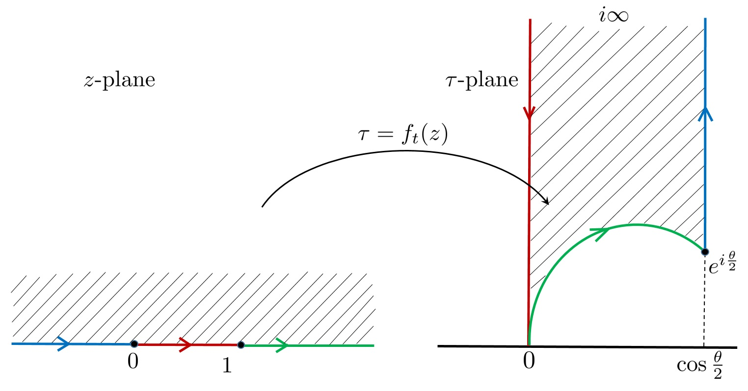
Figure 1. Mapping of the upper half-plane $\mathbb{H}$ onto $\Delta_{t}$ by $f_{t}$.

By Lemma 1, the condition (3.3) becomes $\frac{1}{m_{3}}<1$, i.e., it depends only on the third fixed point $f_{t}(\infty)=e^{i\frac{\theta}{2}}$ and $m_{3}=\frac{1}{1-2t}$ is an integer greater than $1$ including $\infty$ only for $t\in\Big{\{}\frac{1}{2},\frac{1}{3},\frac{1}{4}\Big{\}}$. If $\pi_{t}:\Delta_{t}\rightarrow\mathbb{H}$ is the inverse map of $f_{t}$, then we can extend $\pi_{t}(\tau)$ analytically to a single-valued function on $\mathbb{H}$ with the real axis as its natural boundary by applying the Schwarz reflection principle repeatedly. The covering group of $\pi_{t}$ is the Hecke subgroup $H_{e}(\lambda_{t})$. For more details, see Section 2 of [2], where $H_{e}(\lambda_{t})$ is denoted by $G_{q}$.

The subgroup $H_{e}(\lambda_{t})$ has two cusps and one elliptic point for $t\in\Big{\{}\frac{1}{3},\,\frac{1}{4}\Big{\}}$ and has three cusps for $t=\frac{1}{2}$. Thus, the quotient Riemann surface $H_{e}(\lambda_{t})\backslash\mathbb{H}$ is the two punctured Riemann sphere $\widehat{\mathbb{C}}\setminus\{0,1\}$ for $t\in\Big{\{}\frac{1}{3},\,\frac{1}{4}\Big{\}}$ and the thrice punctured Riemann sphere $\widehat{\mathbb{C}}\setminus\{0,1,\infty\}$ for $t=\frac{1}{2}$. The set of cusps of the Hecke group $H(\lambda_{t})$ is $\mathbb{Q}[\lambda_{t}]\cup\{\infty\}$. To compactify the quotient Riemann surface $H_{e}(\lambda_{t})\backslash\mathbb{H}$, let $\mathbb{H}^{*}=\mathbb{H}\cup\mathbb{Q}[\lambda_{t}]\cup\{\infty\}$. Then, $H_{e}(\lambda_{t})\backslash\mathbb{H}^{*}$ is a compact Riemann surface. For all $\begin{pmatrix}a&b\\ c&d\end{pmatrix}\in H(\lambda_{t})$ and $\tau\in\mathbb{H}$, the meromorphic function $g:\mathbb{H}\rightarrow H(\lambda_{t})\backslash\mathbb{H}^{*}$ is called an automorphic function if $g\bigg{(}\displaystyle\frac{a\tau+b}{c\tau+d}\bigg{)}=g(\tau)$ (see [11]).

4. Proofs of Main Results

Let $\Gamma=\operatorname{PSL}(2,\mathbb{Z})$. For an integer $p>1$, let $M_{p}=\begin{pmatrix}p&0\\ 0&1\end{pmatrix}$, then the transformation group of order $p$ (see Chapter VI of [20]), $\Gamma_{M_{p}}$, is given by

$$\Gamma_{M_{p}}:=\Gamma\cap\Big{(}M_{p}^{-1}\Gamma M_{p}\Big{)},$$

which can be written as the group of Möbius transformations

$$\Gamma_{M_{p}}:=\Big{\{}\gamma\in\Gamma:\hskip 2.84526ptM_{p}\gamma M_{p}^{-1}\in\Gamma\Big{\}}.$$

If $\gamma=\begin{pmatrix}a&b\\ c&d\end{pmatrix}\in\Gamma$, then $M_{p}\gamma M_{p}^{-1}=\begin{pmatrix}a&p\hskip 0.85358ptb\\ \frac{c}{p}&d\end{pmatrix}$. Hence, $M_{p}\gamma M_{p}^{-1}\in\Gamma$ only when $c\equiv 0\,(\text{mod}\,p)$, and we have $\Gamma_{M_{p}}=\Gamma_{0}(p)$. The following lemma is a well-known result, e.g., see Proposition 1.43 in [21] or [20, p. 79].

Lemma 2.

For any positive integer $N$, $\big{|}\Gamma:\Gamma_{0}(N)\big{|}=\Psi(N)$.

Proof of Theorem 1.

For $t\in\Big{\{}\frac{1}{2},\,\frac{1}{3},\,\frac{1}{4}\Big{\}}$ and $\lambda_{t}=2\cos\frac{(1-2t)\pi}{2}$, let

$$H_{M_{p}}(\lambda_{t})=\Big{\{}\gamma\in H_{e}(\lambda_{t}):M_{p}\gamma M_{p}^{-1}\in H_{e}(\lambda_{t})\Big{\}},$$

where $p$ is an integer $>1$ and $M_{p}=\begin{pmatrix}p&0\\ 0&1\end{pmatrix}$. If $\gamma=\begin{pmatrix}a&b\lambda_{t}\\ c\lambda_{t}&d\end{pmatrix}\in H_{e}(\lambda_{t})$, then

$$M_{p}\gamma M_{p}^{-1}=\begin{pmatrix}a&p\hskip 1.42262ptb\lambda_{t}\\ \frac{c}{p}\hskip 1.42262pt\lambda_{t}&d\end{pmatrix}.$$

Therefore, $M_{p}\gamma M_{p}^{-1}\in H_{e}(\lambda_{t})$ only when $c\equiv 0\,(\text{mod }p)$ and we have

(4.1) $$H_{M_{p}}(\lambda_{t})=\Bigg{\{}\begin{pmatrix}a&b\lambda_{t}\\ c\lambda_{t}&d\end{pmatrix}\in H_{e}(\lambda_{t}):c\equiv 0\,(\text{mod }p)\Bigg{\}}.$$

Consequently,

(4.2) $$H_{e}(\lambda_{t})\cap\Big{(}M_{p}^{-1}H_{e}(\lambda_{t})M_{p}\Big{)}=H_{M_{p}}(\lambda_{t})$$

and

$$H_{M_{p}}(\lambda_{t})<H_{e}(\lambda_{t})<H(\lambda_{t}).$$

Let $\pi_{t}$ and $\pi_{t}^{\prime}$ denote the canonical projections $\mathbb{H}\rightarrow H_{e}(\lambda_{t})\backslash\mathbb{H}$ and $\mathbb{H}\rightarrow H_{M_{p}}(\lambda_{t})\backslash\mathbb{H}$, respectively. From the subgroup relation $H_{M_{p}}(\lambda_{t})<H_{e}(\lambda_{t})$, we have the branched covering map $\varphi:H_{M_{p}}(\lambda_{t})\backslash\mathbb{H}\rightarrow H_{e}(\lambda_{t})\backslash\mathbb{H}$ and the following commutative diagram:

The degree of the branched covering $H_{M_{p}}(\lambda_{t})\backslash\mathbb{H}\rightarrow H_{e}(\lambda_{t})\backslash\mathbb{H}$ is $\big{|}H_{e}(\lambda_{t}):H_{M_{p}}(\lambda_{t})\big{|}$, which is the degree $\mu\big{(}p,\frac{1}{t}\big{)}$ in each of $\alpha$ and $\beta$ of the polynomial $P(\alpha,\beta)$ by Theorem A.

Also, for $\Gamma=\operatorname{PSL}(2,\mathbb{Z})$, we have

$$\Gamma\cap\Big{(}M_{p}^{-1}\Gamma M_{p}\Big{)}=\Gamma_{0}(p),$$

and

$$\Gamma_{0}(\lambda_{t}^{2}p)<\Gamma_{0}(\lambda_{t}^{2})<\Gamma.$$

Let us consider the mapping

$$\Theta:H_{e}(\lambda_{t})\rightarrow\Gamma_{0}(\lambda_{t}^{2})$$

defined by

$$\Theta(A)=M_{\lambda_{t}}^{-1}AM_{\lambda_{t}},$$

where $A=\begin{pmatrix}a&b\lambda_{t}\\ c\lambda_{t}&d\end{pmatrix}\in H_{e}(\lambda_{t})$ and $M_{\lambda_{t}}=\begin{pmatrix}\lambda_{t}&0\\ 0&1\end{pmatrix}$. Then, we have

$$\Theta(H_{e}(\lambda_{t}))=\Gamma_{0}(\lambda_{t}^{2})\quad\text{and}\quad\Theta(H_{M_{p}}(\lambda_{t}))=\Gamma_{0}(\lambda_{t}^{2}p).$$

Therefore, $H_{e}(\lambda_{t})\cong\Gamma_{0}(\lambda_{t}^{2})$, $H_{M_{p}}(\lambda_{t})\cong\Gamma_{0}(\lambda_{t}^{2}p)$, and we have

$$\big{|}H_{e}(\lambda_{t}):H_{M_{p}}(\lambda_{t})\big{|} =\big{|}\Gamma_{0}(\lambda_{t}^{2}):\Gamma_{0}(\lambda_{t}^{2}p)\big{|}=\frac{\big{|}\Gamma:\Gamma_{0}(\lambda_{t}^{2}p)\big{|}}{\big{|}\Gamma:\Gamma_{0}(\lambda_{t}^{2})\big{|}}.$$

By Lemma 2, $\big{|}\Gamma:\Gamma_{0}(\lambda_{t}^{2}p)\big{|}=\Psi(\lambda_{t}^{2}p)$ and $\big{|}\Gamma:\Gamma_{0}(\lambda_{t}^{2})\big{|}=\Psi(\lambda_{t}^{2})$. Hence

$$\mu\Big{(}p,\frac{1}{t}\Big{)}=\big{|}H_{e}(\lambda_{t}):H_{M_{p}}(\lambda_{t})\big{|}=\frac{\Psi(\lambda_{t}^{2}p)}{\Psi(\lambda_{t}^{2})},$$

which implies $\mu(p,2)=\frac{1}{6}\Psi(4p)$, $\mu(p,3)=\frac{1}{4}\Psi(3p)$ and $\mu(p,4)=\frac{1}{3}\Psi(2p)$. By (2.1), it is easy to show that $\Psi(4p)=2\Psi(2p)$. Thus, $\mu(p,2)=\mu(p,4)$ as required. $\square$

Let $X_{1}=H_{e}(\lambda_{t})\backslash\mathbb{H}$ and $X_{2}=H_{M_{p}}(\lambda_{t})\backslash\mathbb{H}$. For the canonical projections $\pi_{t}:\mathbb{H}\rightarrow X_{1}$ and $\pi_{t}^{\prime}:\mathbb{H}\rightarrow X_{2}$, consider the mappings $\varphi:X_{2}\rightarrow X_{1}$ and $\psi:X_{2}\rightarrow X_{1}$ such that $\pi_{t}=\varphi\circ\pi_{t}^{\prime}$ and $\pi_{t}\circ M_{p}=\psi\circ\pi_{t}^{\prime}$, i.e., the following diagrams commute:

            

Thus, for $z\in X_{2}$, the solution $(\alpha,\beta)$ to the generalized modular equation (1.1) is parametrized by $\alpha=\varphi(z)$ and $\beta=\psi(z)$. Before giving the proofs of Theorems 2 and 3, we recall the following two lemmas from [2].

Lemma 3 ([2, Lemma 2.3]).

For an integer $p>1$, let $t\in(0,\frac{1}{2}]$ and $M_{p}=\begin{pmatrix}p&0\\ 0&1\end{pmatrix}$. If $H_{e}^{\prime}(\lambda_{t})=M_{p}^{-1}H_{e}(\lambda_{t})M_{p}$ and $H_{M_{p}}(\lambda_{t})=H_{e}(\lambda_{t})\cap H_{e}^{\prime}(\lambda_{t})$, then

$$\big{|}H_{e}(\lambda_{t}):H_{M_{p}}(\lambda_{t})\big{|}=\big{|}H_{e}^{\prime}(\lambda_{t}):H_{M_{p}}(\lambda_{t})\big{|}.$$

Lemma 4 ([2, Lemma 3.4]).

Let $W_{p}=\begin{pmatrix}0&-1\\ p&0\end{pmatrix}$ and $\tau\in\mathbb{H}$, then $W_{p}\tau=\displaystyle-\frac{1}{p\tau}$ induces an automorphism $\omega$ on $X_{2}$ such that $\pi_{t}^{\prime}\circ W_{p}=\omega\circ\pi_{t}^{\prime}$ and $\psi=1-\varphi\circ\omega$.

Now, we are ready to prove Theorems 2 and 3.

Proof of Theorem 2.

First, recall that the covering group of the map $\pi_{t}$ is the Hecke subgroup $H_{e}(\lambda_{t})$ and it is well-known that the index of $H_{e}(\lambda_{t})$ in the Hecke group $H(\lambda_{t})$ is 2 (see [12, p. 61]). Thus, $\Gamma_{1}=H_{e}(\lambda_{t})$ and $(i)$ follows easily from this fact.

From (4.2), we have $\Gamma_{2}=\Gamma_{1}\cap\big{(}M_{p}^{-1}\Gamma_{1}M_{p}\big{)}=H_{M_{p}}(\lambda_{t})$. By virtue of the proof of Theorem 1, we have $\Gamma_{2}\cong\Gamma_{0}(\lambda_{t}^{2}p)$, and hence, $\Gamma_{2}$ is isomorphic to $\Gamma_{0}(4p)$, $\Gamma_{0}(3p)$ and $\Gamma_{0}(2p)$ for $t=\frac{1}{2},\frac{1}{3}$ and $\frac{1}{4}$, respectively. Each of $\Gamma_{0}(4p)$, $\Gamma_{0}(3p)$ and $\Gamma_{0}(2p)$ has finite index in $\Gamma=\operatorname{PSL}(2,\mathbb{Z})$. Therefore, $\Gamma_{2}$ has finite index in $H(\lambda_{t})$, which implies $(ii)$.

If $X_{1}=\Gamma_{1}\backslash\mathbb{H}$ and $X_{2}=\Gamma_{2}\backslash\mathbb{H}$, then the degree of the branched covering $\varphi:X_{2}\rightarrow X_{1}$ is equal to the index of $\Gamma_{2}$ in $\Gamma_{1}$. Since each of $\Gamma_{1}$ and $\Gamma_{2}$ has finite index in $H(\lambda_{t})$, the index of $\Gamma_{2}$ in $\Gamma_{1}$ is finite. Therefore, $(iii)$ holds.

It is not difficult to prove that $\alpha(\tau)$ and $\beta(\tau)=\alpha(p\tau)$ are automorphic functions on $\Gamma_{1}$ and $\Gamma_{1}^{\prime}:=M_{p}^{-1}\Gamma_{1}M_{p}$, respectively. Recall that the quotient Riemann surface $X_{1}=\Gamma_{1}\backslash\mathbb{H}$ is $\widehat{\mathbb{C}}\setminus\{0,1\}$ for $t\in\Big{\{}\frac{1}{3},\,\frac{1}{4}\Big{\}}$ and $\widehat{\mathbb{C}}\setminus\{0,1,\infty\}$ for $t=\frac{1}{2}$. If $\widehat{X}_{1}$ is the compactification of $X_{1}$, then $\widehat{X}_{1}$ is the Riemann sphere $\widehat{\mathbb{C}}$. Thus, the field of automorphic functions for $\Gamma_{1}$ is $\mathbb{C}(\alpha(\tau))$. If $X_{1}^{\prime}=\Gamma_{1}^{\prime}\backslash\mathbb{H}$ and $\widehat{X}_{1}^{\prime}$ is the compactification of $X_{1}^{\prime}$, then $\widehat{X}_{1}^{\prime}=\widehat{\mathbb{C}}$. The field of automorphic functions for $\Gamma_{1}^{\prime}$ is $\mathbb{C}(\beta(\tau))$. Since $\Gamma_{2}<\Gamma_{1}$ and $\Gamma_{2}<\Gamma_{1}^{\prime}$, both $\mathbb{C}(\alpha(\tau))$ and $\mathbb{C}(\beta(\tau))$ are subfields of the field of automorphic functions for $\Gamma_{2}=\Gamma_{1}\cap\Gamma_{1}^{\prime}$, i.e., $\mathbb{C}(\alpha(\tau),\beta(\tau))$. If $\mu=\big{|}\Gamma_{1}:\Gamma_{2}\big{|}$, then $\varphi:X_{2}\rightarrow X_{1}$ is a $\mu$-sheeted branched covering map. For any function $g\in\mathbb{C}(\alpha(\tau))$, we have a function $f\in\mathbb{C}(\alpha(\tau),\beta(\tau))$ by virtue of the pullback $\varphi^{*}(g)=g\circ\varphi=f$, where $\varphi^{*}:\mathbb{C}(\alpha(\tau))\rightarrow\mathbb{C}(\alpha(\tau),\beta(\tau))$ is an algebraic field extension of degree $\mu$ (see [15, Theorem 8.3]). Similarly, if $\psi$ is the branched covering map $X_{2}\rightarrow X_{1}^{\prime}$, then $\psi$ is also a $\mu$-sheeted covering map, since $|\Gamma_{1}^{\prime}:\Gamma_{2}|=\mu$ by Lemma 3. Hence, $\psi^{*}:\mathbb{C}(\beta(\tau))\rightarrow\mathbb{C}(\alpha(\tau),\beta(\tau))$ is an algebraic field extension of degree $\mu$. Consequently, there is a polynomial $P(\alpha(\tau),\beta(\tau))$ which has degree $\mu$ in each of $\alpha(\tau)$ and $\beta(\tau)$. The polynomial $P(\alpha(\tau),\beta(\tau))$ is determined up to a scalar factor so that $P(\alpha(\tau),\beta(\tau))=0$, which implies $(iv)$ and completes the proof. $\square$

Recall that the Hecke subgroup $H_{M_{p}}(\lambda_{t})$ is given by

$$H_{M_{p}}(\lambda_{t})=\Bigg{\{}\begin{pmatrix}a&b\lambda_{t}\\ c\lambda_{t}&d\end{pmatrix}\in H_{e}(\lambda_{t}):c\equiv 0\,(\text{mod }p)\Bigg{\}}.$$

Let $W_{p}=\begin{pmatrix}0&-1\\ p&0\end{pmatrix}$, then

(4.3) $$W_{p}^{-1}\begin{pmatrix}a&b\lambda_{t}\\ c\lambda_{t}&d\end{pmatrix}W_{p}=\begin{pmatrix}d&-\frac{c}{p}\lambda_{t}\\ -pb\lambda_{t}&a\end{pmatrix},$$

where $\begin{pmatrix}a&b\lambda_{t}\\ c\lambda_{t}&d\end{pmatrix}\in H_{M_{p}}(\lambda_{t})$.

Proof of Theorem 3.

Since $c\equiv 0\,(\text{mod }p)$, it follows from (4.3) that

$$W_{p}^{-1}\begin{pmatrix}a&b\lambda_{t}\\ c\lambda_{t}&d\end{pmatrix}W_{p}\in H_{M_{p}}(\lambda_{t}).$$

Thus, $H_{M_{p}}$ is normalized by $W_{p}$ in $\operatorname{PSL}(2,\mathbb{R})$. The Möbius transformation $W_{p}\tau=-\displaystyle\frac{1}{p\tau}$ induces an automorphism $\omega$ on $X_{2}=H_{M_{p}}\backslash\mathbb{H}$ such that the following diagram commutes:

Moreover, by Lemma 4, $\omega:X_{2}\rightarrow X_{2}$ satisfies the following functional equations:

$$\varphi\circ\omega=1-\psi,$$

$$\psi\circ\omega=1-\varphi.$$

Hence, for $z\in X_{2}$, we have $\varphi(\omega(z))=1-\psi(z)=1-\beta$ and $\psi(\omega(z))=1-\varphi(z)=1-\alpha$, i.e., $\omega$ interchanges $\alpha$ and $1-\beta$, and $\beta$ and $1-\alpha$. Thus, we deduce that $(1-\beta,1-\alpha)$ is also a solution to (1.1) and $P(1-\beta,1-\alpha)=0.$

$\square$

References

• [1] Md. S. Alam, A Geometric Study on Ramanujan’s Modular Equations and Hecke Groups, Ph. D. Thesis, Tohoku University, 2021.
• [2] Md. S. Alam, T. Sugawa, \sayGeometric deduction of the solutions to modular equations, The Ramanujan Journal 59(2) (2022), 459–477.
• [3] G. D. Anderson, S.-L. Qiu, M. K. Vamanamurthy, M. Vuorinen, \sayGeneralized elliptic integrals and modular equations, Pacific J. Math. 192 (2000), 1–37.
• [4] G. D. Anderson, T. Sugawa, M. K. Vamanamurthy, M. Vuorinen, \sayTwice-punctured hyperbolic sphere with a conical singularity and generalized elliptic integral, Math. Z. 266 (2010), 181–191.
• [5] G. D. Anderson, M. K. Vamanamurthy, M. K. Vuorinen, Conformal Invariants, Inequalities, and Quasiconformal Maps, Wiley-Interscience, 1997.
• [6] H. Bateman, Higher Transcendental Functions, Vol. I, McGraw-Hill, New York, 1953.
• [7] B. C. Berndt, Ramanujan’s Notebooks, Part III, Springer-Verlag, New York, 1991.
• [8] B. C. Berndt, Number Theory in the Spirit of Ramanujan, Amer. Math. Soc., Providence, RI, 2006.
• [9] B. C. Berndt, S. Bhargava, F. G. Garvan, \sayRamanujan’s theories of elliptic functions to alternative bases, Trans. Amer. Math. Soc. 347 (1995), 4163–4244.
• [10] J. M. Borwein, P. B. Borwein, Pi and the AGM, Wiley, New York, 1987.
• [11] D. Bump, Automorphic Forms and Representations, Cambridge Studies in Advanced Mathematics 55, Cambridge University Press, Cambridge, 1997.
• [12] İ. N. Cangül, D. Singerman, \sayNormal subgroups of Hecke groups and regular maps, Math. Proc. Camb. Phil. Soc. 123 (1998), 59–74.
• [13] H. H. Chan, W.-C. Liaw, \sayOn Russell-type modular equations, Can. J. Math. 52 (2000), 31–46.
• [14] L. E. Dickson, History of the Theory of Numbers, Vol. I. Divisibility and Primality, Chelsea Publishing Company, New York, 1952.
• [15] O. Forster, Lectures on Riemann Surfaces, Springer-Verlag, New York, 1981.
• [16] S. Katok, Fuchsian Groups, The University of Chicago Press, Chicago and London, 1992.
• [17] Z. Nehari, Conformal Mapping, McGraw-Hill, New York, 1952.
• [18] R. Russell, \sayOn $\kappa\lambda$-$\kappa^{\prime}\lambda^{\prime}$ modular equations, Proc. London Math. Soc. 19 (1887), 90–111.
• [19] G. Sansone, J. Gerretsen, Lectures on the Theory of Functions of a Complex Variable, Vol. II. Geometric Theory, Wolters-Noordhoff Publ., Groningen, 1969.
• [20] B. Schoeneberg, Elliptic Modular Functions, Springer-Verlag, Berlin, Heidelberg, New York, 1974.
• [21] G. Shimura, Introduction to the Arithmetic Theory of Automorphic Functions, Princeton University Press, Princeton, New Jersey, 1971.
• [22] E. T. Whittaker, G. N. Watson, A Course of Modern Analysis, 4th ed., Cambridge University Press, Cambridge, 1927.