REFINE2: A tool to evaluate real-world performance of machine-learning based effect estimators for molecular and clinical studies

Abstract

Data-adaptive (machine learning-based) effect estimators are increasingly popular to reduce bias in high-dimensional bioinformatic and clinical studies (e.g. real-world data, target trials, -omic discovery). Their relative statistical efficiency (high power) is particularly invaluable in these contexts since sample sizes are often limited due to practical and cost concerns. However, these methods are subject to technical limitations that are dataset specific and involve computational trade-offs. Thus, it is challenging for analysts to identify when such methods may offer benefits or select amongst statistical methods. We present extensive simulation studies of several cutting-edge estimators, evaluating both performance and computation time. Critically, rather than use arbitrary simulation data, we generate synthetic datasets mimicking the observed data structure (plasmode simulation) of a real molecular epidemiologic cohort. We find that machine learning approaches may not always be indicated in such data settings, but that performance is highly context dependent. We present a user-friendly Shiny app REFINE2 (Realistic Evaluations of Finite sample INference using Efficient Estimators) that enables analysts to simulate synthetic data from their own datasets and directly evaluate the performance of several cutting-edge algorithms in those settings. This tool may greatly facilitate the proper selection and implementation of machine-learning-based effect estimators in bioinformatic and clinical study contexts.

Keywords: doubly robust, crossfit, augmented inverse probability weighting (AIPW), targeted minimum loss estimation (TMLE), bioinformatics, target trial, molecular epidemiology, high-dimension, plasmode, SuperLearner, misspecification, finite samples, simulation

1 Introduction

The proper application of machine learning to infer biological effects from multiomic data presents an on-going challenge in bioinformatic and clinical studies (Libbrecht and Noble (2015), Hill et al. (2016), Li et al. (2010), Wang and Wu (2019), Larrañaga et al. (2006), Lecca (2021),Prosperi et al. (2020), Park and Kellis (2021)). Estimation of treatment effects via data-adaptive, efficient estimators such as Targeted Minimum Loss Estimation (Díaz and van der Laan (2017), Díaz (2020)) and related approaches to model and compute counterfactual quantities based on Bayesian networks have risen as state-of-the-art in both genomic (Gruber and van der Laan (2010), Ness et al. (2016), White and Vignes (2019)) and medical applications (Balzer et al. (2016), Kreif et al. (2017), Sofrygin et al. (2019), Rossides et al. (2021), Huang et al. (2021)). They may be used to augment real-world evidence "target trial" studies (Dickerman et al. (2019), Challa et al. (2020)) but are particularly beneficial in typical high dimensional setting presented by molecular and bioinformatic studies (Pang et al. (2016a), Ju et al. (2019)).

However, recent applications have also called into question the reliability of such approaches in real-world data (Yu et al. (2019)). To estimating causal effect parameters, the use of doubly-robust (DR) efficient estimators (Augmented Inverse Probability Weighting, AIPW; Targeted Minimum Loss Estimation, TMLE) coupled with ensemble learning of nuisance parameters has attracted much deserved attention (Naimi et al. (2021), Balzer and Westling (2021), Rotnitzky et al. (2019), Pang et al. (2016b)). The main features of robustness to either treatment or outcome model mis-specification and the ability to overcome slower convergence rates of data-adaptive algorithms (i.e. flexible, non-smooth, "machine learning") are key practical features recommending their uptake for observational clinical research settings, where covariate data will be abundant, but model mis-specification (e.g. functional forms and/or variable selection) is nearly assured.

Recent works have highlighted some core considerations for investigators planning to apply these methods. These include the insufficiency of singly-robust methods to achieve bias minimization Naimi et al. (2021) and the need for crossfitting, i.e., target parameter and standard error estimation on separate datasets from nuisance function estimation (Newey and Robins (2018), Zivich and Breskin (2021)) to produce valid standard errors, even when treatment or outcome models are slightly mis-specified. Technically, this occurs when algorithms that are highly data-adaptive do not fulfill Donsker conditions necessary for semi-parametric estimation, resulting in an asymptotically non-negligible empirical process bias. Since such algorithms are difficult to classify, for simplicity, we will refer (somewhat imprecisely) to algorithms that likely violate these conditions, such as random forests or boosted regression trees, as non-smooth, data-adaptive, flexible, or "machine learning," interchangeably. We will refer to algorithms that are likely to suffice, such as penalized linear regression and multivariate polynomial splines, as smooth (differentiable) algorithms.

More fundamentally, small real-world sample sizes general prevent any guarantees of appropriate coverage properties regardless of the types of estimators implemented (Benkeser et al. (2017), Rotnitzky et al. (2019), Balzer and Westling (2021)). For example, Benkeser et al. (2017) demonstrated an approach for doubly robust inference, i.e. nominal asymptotic coverage when using non-smooth estimators. However, performance in small sample ($n<500$) remained sub-optimal. Nonetheless, the implementation of double-crossfit, doubly-robust estimators with sufficiently diverse flexible estimation of nuisance parameters have appeared in these studies to have optimal bias and variance properties amongst possible alternatives even amongst small sample sizes (Balzer and Westling (2021)). As Balzer and Westling (2021) points out, however, these work have generally evaluated estimators on simple data sets that differ in critical ways from typical data and model-fitting procedures applied in clinical and other biomedical contexts. For example, in molecular epidemiologic settings measured covariates will be high-dimensional, while cohort sizes will be moderate due to cost and logistical challenges of follow-up and measurement. Assessing performance in simulated data sets as close to the target context as possible is especially critical (Morris et al. (2019), Boulesteix et al. (2017), Stokes et al. (2020)) when complex data present many identification and estimation threats, including conditions not often considered, such as inclusion of inappropriate (e.g. near-instruments) or excess covariates irrelevant to the data generating process. Given the major promise of doubly-robust methods in performance under model misspecification, particularly the optimization of nuisance models through data-adaptive ML approaches, properly modeling the target analytic context (i.e. data structure with relevant features) is key. Evaluation of these methods against standard approaches in more representative data settings will give a better sense of their potential real-world performance.

Previous simulation studies have used fairly simple confounding structures (Naimi et al. (2021)) and generally large sample sizes (Bahamyirou et al. (2019), Zivich and Breskin (2021)) to clearly demonstrate and isolate certain threats to estimators. However, such settings may be overly optimistic in terms of both data structures and model-fitting practices in clinical and molecular epidemiologic settings. In the latter settings, practical concerns such as overadjustment of high-dimension covariates (i.e. adjustment of near-instruments), practical positivity violations, small samples, and mis-specification of average treatment effects, e.g. by omission of key biological interactions, will be common. Moreover, the typical applied researcher may not be able to spend much time tuning algorithmic hyper-parameter, an important factor even in ensemble learning performance Naimi et al. (2021). One past effort by Bahamyirou et al. (2019) focusing on positivity violations in propensity score estimation also only considered large samples and few, simple covariates, and only used an approach to address propensity score fitting (collaborative-TMLE; CTMLE van der Laan and Gruber (2010)) and not cross-fitting of the overall estimator. Work by Pang, et al (Pang et al. (2016b)) utilized a covariate structure-preserving "plasmode" simulation method (e.g. Franklin et al. (2014)) to evaluate TMLE in the presence of high dimensional covariates. However, the work was conducted in the context of large administrative pharmacoepidemiologic databases (N >16,000) and did not consider non-smooth learning nuisance parameter a key value of efficient estimators. Taken together, these results present an optimistic picture of the robustness of novel estimators that may not apply to all observational health research settings.

In this paper, we demonstrate performance in closer to real-world conditions for clinical and molecular epidemiologic studies, which could greatly benefit from the efficiency and robustness properties of newer estimators. Notably, we apply efficient estimators (AIPW, TMLE) with ensemble learning of nuisance parameters to estimate average treatment effects under various scenarios of mis-specification. We fit models with and without double-crossfitting and with smooth and/or non-smooth algorithms. Covariate data were drawn from an existing longitudinal cohort study (N = 1178; 331 covariates) to simulate treatment and outcome values under user-specified models ("plasmode" simulation). We then present a tool REFINE2 (A tool to evaluate real-world performance of machine-learning based effect estimators for molecular and clinical studies) which automates this process by taking user input datasets, generating synthetic data with fixed effect sizes, and testing various machine-learning based estimators under user-specified conditions.

The organisation of the paper is as follows: In Section 2, we introduce the estimand of interest and estimators we will be comparing. Section 3 replicates a classic simulation study demonstrating the basic properties of these estimators under model mis-specification, and confirming their good asymptotic performance in basic simulated data. In Section 4, we describe the overall simulation method and the three scenarios we simulated from existing cohort data. In Section 5 we present the results of the analyses and in Section 6 discuss implications and give final recommendations.

2 Methods

2.1 The Target Parameter

We use the Rubin counterfactual framework to define the causal estimand: Suppose we observe $n$ i.i.d. data $(O_{1},O_{2},...,O_{n})$. Each observation $O_{i}$ consists of $(W_{i},A_{i},Y_{i})$, where $Y_{i}\in\mathbb{R}$ denotes the observed outcome, $A_{i}\in\{0,1\}$ is a binary random variable representing the treatment received, and $W_{i}\in\mathcal{W}\subset\mathbb{R}^{d}$ denotes the covariates of $i$th subject. Furthermore, we denote the counterfactuals as $Y(a),a=0,1$. Each counterfactual $Y(a)$ representing the outcome received has the patient received the treatment $a$.

The average treatment effect (ATE) is then defined as:

$$\psi_{0}=E[Y(1)]-E[Y(0)]$$

To identify the ATE, we also adopt the following causal assumptions:

• Exchangeability: $(Y(1),Y(0))\bot A|P(A=1|W)$, where W is the vector of all confounding variables

• Consistency: If $A=a$, then $Y(a)=Y$; that is, the observed value of Y at a is equal to potential outcome of $Y$ had $A$ been set to $a$.

• Stable Unit Treatment Values Assumption (SUTVA): No interference between units.

• Structural positivity holds: $P(X=1|W=w)>0$ and $P(X=0|W=w)>0$ for all units where $w\in\mathcal{W}$

Based on these assumptions, we can identify the ATE as

$$\psi_{0}=E[E[Y|A=1,W]-E[Y|A=1,W]]$$

2.2 Propensity Score and IPTW

A conventional approach to exchangeability is via Inverse Probability of Treatment Weighting (IPTW) to form pseudo populations where treatment status is conditionally independent of measured predictors. Based on Rosenbaum and Rubin (1983) $(Y(1),Y(0))\bot A|P(A=1|W)$ under strong exchangeability and positivity. Namely, confounding may be controlled by weighting individual observations by the inverse of their propensity score $g_{0}(W)=P(A=1|W)$: $1/g_{0}(W)$ for the treated, $1/(1-g_{0}(W))$ for the control. This is sometimes referred also as Horvitz-Thompson (HT) estimator Horvitz and Thompson (1952). It is a consistent estimator of the IP weighted mean as long as the estimated propensity score (PS) model $\hat{g}$ is correctly specified. The IPW estimator of the ATE is then given by:

$$\hat{\psi}_{n}^{IPW}=\frac{1}{n}\sum_{i=1}^{n}\frac{A_{i}Y_{i}}{\hat{g}(W_{i})}-\frac{1}{n}\sum_{i=1}^{n}\frac{(1-A_{i})Y_{i}}{1-\hat{g}(W_{i})}$$

Highly discriminating propensity scores can lead to extreme weights, so a general approach is to scale or stabilize all weights by introducing the observed treatment prevalence $P(A=1)$ to the numerator. As classification improves, so does the presence of extreme weights, particularly in high dimensional settings. Probabilities that are close to 0 or 1 may result in near violation of the positivity assumption, resulting in bias and instability in ATE and variance estimation. We adopt the standard practice of truncating extreme weights to the upper and lower 5%-iles, trading off some misspecification to improve performance. Approaches to iterative fitting of high-dimensional propensity scores with smooth or more flexible estimators are possible (e.g. Schneeweiss et al. (2009), Koch et al. (2017), Wyss et al. (2018))

2.3 g-computation

A second standard approach is the g-computation estimator, which is motivated directly by the ATE identification form known as the G-formula, $E[E[Y|A=1,W]-E[Y|A=0,W]]$. The ATE is estimated by first fitting the outcome model (OM) for the outcome $Y$ conditional on the treatment variable $A$ and covariates $W$. Then, the predicted outcome value for each observation is computed at the assigned treatment value and the treatment-specific mean computed. This is repeated for the control or comparison treatment value and the ATE is given by the difference in mean outcome for the sample population under the counterfactual treatment values (e.g. treatment and control). More specifically,

$$\hat{\psi}_{n}^{gcomp}=\frac{1}{n}\sum_{i=1}^{n}m_{1}(W_{i})-\frac{1}{n}\sum_{i=1}^{n}m_{0}(W_{i})$$

where $m_{i}(w)=\hat{E}[Y|X=i,W=w]$. As with IPTW, the OM can be fitted with smoothly or more flexible models, though the latter is not recommended (Naimi et al. (2021)). The non-parametric bootstrap is typically used to estimate percentile-based standard errors.

2.4 Doubly-robust, efficient estimators: TMLE and AIPW

Approaches combining both propensity score (PS) and outcome models (OM) such as Targeted Maximum Likelihood (or Minimum Loss) Estimation (TMLE) and Augmented Inverse Probability Weighting (AIPW) are often termed "doubly-robust" estimators. That is, estimation of counterfactual contrasts such as the ATE are consistent (asymptotically unbiased) as long as at least one of the two models (PS or OM) are correctly specified. In this context, the estimated PS (or clever covariate) or OM-based predictor (or offset) are considered to be "nuisance" parameters in that they are not the primary parameters of interest. Nuisance parameters may be fitted by one or more smooth or flexible, data-adaptive algorithms without substantial alterations to the final estimator. In theory, the latter particularly allows for more complete adjustment for confounding or compensation for model misspecification without added complexity to the final estimator. Importantly, these doubly-robust estimators are necessary to compensate for the relatively slower rates of convergence for flexible estimators (even when models are correctly specified). However, as will be discussed in this paper, these approaches may suffer additional limitations in practical application.

AIPW, also referred to as a one-step correction estimator, is developed based on g-computation with a mean-zero correction term based on the PS for the asymptotic bias arising from an inconsistent (biased) OM model. Predicted probabilities by PS model and outcome by OM are added together to generate predictions of ATE under each value of covariate. More specifically,

$$\hat{\psi}_{n}^{AIPW}=\frac{1}{n}\sum_{i=1}^{n}(\frac{A_{i}Y_{i}}{\hat{g}(W_{i})}-\frac{A_{i}-\hat{g}(W_{i})}{\hat{g}(W_{i})}m_{1}(W_{i}))-\frac{1}{n}\sum_{i=1}^{n}(\frac{(1-A_{i})Y_{i}}{1-\hat{g}(W_{i})}+\frac{A_{i}-\hat{g}(W_{i})}{1-\hat{g}(W_{i})}m_{0}(W_{i}))$$

Standard errors and confidence intervals can be estimated by from the fitted influence functions (Lunceford and Davidian (2004)) or by bootstrap (Funk et al. (2011))

TMLE targets the estimation of ATE by correcting the asymptotic bias of g-computation estimator by adjusting the distribution (Schuler and Rose (2017)) in a slightly different manner than AIPW.

First, a initial prediction of the outcome Y (scaled to [0,1] for continuous Y) is fitted by the OM ($m_{1}$ and $m_{0}$). Next, a smooth submodel with a single parameter estimated by the PS ("clever covariate") with an offset comprising the initial prediction. Specifically, we denote the clever covariate as:

$$H\left(A_{i},W_{i}\right)=\frac{A_{i}}{\hat{g}(W_{i})}-\frac{1-A_{i}}{1-\hat{g}(W_{i})}$$

The submodel indexed by $\epsilon$ is obtained by fitting the logistic regression

$$\operatorname{logit}\left(Y_{i}\right)=\operatorname{logit}\left(m_{A_{i}}(W_{i})\right)+\epsilon H\left(A_{i},W_{i}\right)$$

The fitted submodel is then used to compute predicted outcome for each treatment level, and average difference of them produces the estimated ATE.

$$\operatorname{logit}(m_{a}^{*}(W_{i}))=\operatorname{logit}(m_{a}^{*}\left(m_{a},H\left(a,W_{i}\right),\hat{\epsilon}\right))=\operatorname{logit}\left(m_{a}\left(W_{i}\right)+\hat{\epsilon}H\left(a,W_{i}\right)\right),a=0,1$$

$$\hat{\psi}_{TMLE}=\frac{1}{n}\sum_{i}^{n}(m_{1}^{*}(W_{i})-m_{0}^{*}(W_{i}))$$

Standard errors and confidence intervals can again be estimated from fitted influence functions.

2.5 Double Cross-Fit (DC)

A major challenge to doubly-robust estimators arises when flexible, non-smooth estimators are used to fit high-dimensional nuisance functions when target parameters are of low dimensions, as is often the case with applications of AIPW and TMLE. Notably, the rate of bias reduction in the empirical process term (Benkeser et al. (2017)) with increasing sample size is insufficient when non-smooth (specifically non-Donsker class) algorithms are applied, leading to asymptotic bias. To address this, cross-fitting procedures were proposed (Chernozhukov et al. (2018) Newey and Robins (2018)) wherein K-fold splits of the data are used to independently fit nuisance models and the final estimator. This approach is asymptotically unbiased if both OM and PS models are correctly specified, as demonstrated in Zivich and Breskin (2021), and can be further doubly robust to variance estimation with some modification. Regardless, even with correctly specified models, bias and under-coverage are possible in small (e.g. N < 2000) sample sizes (Benkeser et al. (2017), Balzer and Westling (2021)). Even with small samples (N = 200), it has been suggested but not extensively evaluated that efficient estimators fit with flexible algorithms may outperform smooth learners (Balzer and Westling (2021)).
In this paper, we investigate this finite-sample performance more closely in simulated data more congenial to real clinical and molecular epidemiologic settings. We apply the double cross-fit (DC) (Zivich and Breskin (2021) Newey and Robins (2018)), namely: We separate the data into three equal size random splits. We estimate the OM on split 1, PS model on split 2, then estimate the ATE using split 3. We then rotate the roles of these splits under the constraint that no split is appointed with the same role twice. This produces three different estimators and three split-specific ATE estimates, which are then summarized by a simple mean. To account for stochastic variations in sample splits, we repeat this split-and-estimate process 5 times and take the median as the final ATE estimate. We also investigate whether number of splits (or number of cross-validation folds for ensemble learners substantially influence results).

3 Simulation

3.1 Data Generation

Our primary aim was to demonstrate the relative performance of old and novel ATE estimators on more realistic data sets than those used in past simulation studies, paying particular attention to the relative improvement of flexible, non-smooth algorithms. To benchmark our estimator setup, we replicate the qualitative results of past simulation studies using a common "hard" data generating process (DGP) whose ATE is difficult to estimate with standard smooth approaches (and therefore flexible estimators are favored). Notably, to evaluate that any difference in performance is not strictly due to finite sample bias, we draw a smaller sample than most previous studies, N = 600 to be more comparable to our real data scenario. In this section, we present the set-up and results of this simulation scenario as a baseline to compare across different methods. This DGP appeared first at Kang et al. (2007) and is frequently used to test estimators for ATE because of the extreme non-linear relationship among covariates in both PS and OM (Ning et al. (2020), Benkeser et al. (2020), Funk et al. (2011), Naimi et al. (2021)).

The data generating process consists of simulating N = 600 rows/observations of: 5 confounders $W=(W_{1},W_{2},W_{3},W_{4},W_{5})$ generated as follows:

$$W_{1}\sim N(0,1),\quad W_{2}\sim N(W_{1}+2,2)$$

$$W_{3}\sim N(2,|2W_{2}|),\quad W_{4}\sim N(W_{2}^{2}+2W_{3},|W_{1}|)$$

$$W_{5}\sim N(W_{3}W_{4},|W_{2}-W_{1}|).$$

. A binary exposure variable $A$ generated by logistic regression:

$$P(A=1|W)=\text{logis}(W_{1}+W_{2}/20+W_{3}/50+W_{4}/200+W_{5}/5000)$$

A continuous counterfactual outcome $Y(a),a=0,1$ generated by the following:

$$Y(a)=6.6a+10W_{1}+0.5W_{2}^{2}+0.66W_{3}+0.25W_{4}+0.01W_{3}W_{4}+8\log(W_{5})+N(0,4^{2})$$

Thus here, the true ATE is fixed to be 6.6.

Finally, the observed outcome variable $Y$ is generated by:

$$Y=A\cdot Y(1)+(1-A)\cdot Y(0)$$

3.2 Estimation

To estimate the ATE for this dataset, we fit IPTW, g-computation, AIPW (standard and cross-fit), and TMLE (standard and cross-fit) estimators using a linear regression model for the OM $E[Y|A=a,W]=\alpha_{0}+\alpha_{1}W_{1}+...+\alpha_{5}W_{5}$ and logistic regression for the PS $\text{logit}(P(A=1|W))=\beta_{0}+\beta_{1}W_{1}+...+\beta_{5}W_{5}$ including as covariates $W_{1},...,W_{5}$. Note that absent specifications of covariate interactions and non-linearities, these models would be misspecified.

We then consider different nuisance parameter estimation methods for $E[Y|A=a,W]$ and $P(A=1|W)$ including:

• GLM only

• Cross-validated ensemble learner (SuperLearner) Van der Laan et al. (2007) with a smooth library: GLM, LASSO, multivariate polynomial splines

• Cross-validated ensemble learner (SuperLearner) with a non-smooth library: xgboost and random forest

For simplicity, for each ATE and nusiance parameter estimator combination, we apply the same estimation approach to both OM and PS (e.g. GLM for OM and GLM for PS). For each estimate, we present the absolute bias (Estimate - True), standard error (SE) and 95% confidence interval coverage. For presentation purposes, absolute bias is scaled by 100 in tables. For example, a bias of 1.0 in tables = 0.01 in absolute bias

3.3 Result

The result here, presented in table 1, re-affirms that in the case of small sample and limited covariates with non-linear relationships, using non-smooth learners to predict the treatment mechanism (PS) in a singly-robust (IPTW) setting is suboptimal, largely due to over fitting on the propensity score which induces large weights and non-positivity. Moreover, as also shown in Zivich and Breskin (2021), Naimi et al. (2021), efficient estimators fit with non-smooth algorithms suffer without cross-fitting. Despite the relative small sample size cross-fit estimators using non-smooth libraries perform relatively well and comparable to the models fit with smooth algorithms. Interestingly, standard g-computation performance was ideal potentially due to better congeniality to the simulation data generating process and instability of the PS (Robins et al. (2007), Chatton et al. (2020)). As the focus is on flexible algorithms and efficient estimators rather than of a feature of the simulation, we omit g-computation from subsequent simulation studies.

In the section below, we evaluate whether such qualitative results hold in more realistic finite sample settings with high-dimensional, correlated covariates and various degrees of model misspecification, including the presence of true biological interaction (effect modifiers). We investigate specifically whether crossfitting and non-smooth approaches, which substantially increase computational time, provide improved performance over singly-fit efficient estimators or more conventional regression-based approaches.

Table 1: Result from Plasmode simulation on bias, mean squared error (MSE) and 95% confidence interval (CI) coverage.

	IPW	TMLE		AIPW		DC-TMLE		DC-AIPW
		S	NS	S	NS	S	NS	S	NS
Bias ($\times$ 100)	-7.56	0.3	0.03	0.35	0.34	0.14	0.36	0.23	0.08
SE ($\times$ 100)	37.85	8	7.08	8.25	7.14	9.28	9.23	9.3	9.36
CI covg.	0.99	0.92	0.87	0.94	0.92	0.96	0.95	0.95	0.98
MSE	0.1	0.01	0.02	0.01	0.01	0.01	0.01	0.01	0.01
BVar	0.1	0.01	0.02	0.01	0.01	0.01	0.01	0.01	0.01

4 Plasmode

4.1 Source data and plasmode simulation approach

To generate our data generating process, we borrow covariate data from the Growing Up in Singapore Towards healthy Outcomes (GUSTO) prospective birth cohort (Soh et al. (2014)), a population-based, deeply genotyped and phenotyped mother-offspring longitudinal cohort designed to investigate genetic, environmental, and behavioral influences on child and adolescent physical and mental health. The dataset has $n=1178$ observations and covariates of dimension $p=331$ consisting of genetic and other molecular biomarkers (e.g. micronutrients), sociodemographic characteristics, behavioral measures, clinical measurements, and medical history data. Variable identities were anonymized as they were not material to the data generating process, though variables plausibly related to effect measure modification (e.g. ethnicity and sex were noted for simulation purposes). To simplify the simulation task, a single imputation set by multivariate iterated regressions (i.e. chained equations) was taken to form a complete case starting set. A simple exploratory analysis can be found in appendix.

We specified a scientific task of estimating the ATE of maternal pre-pregnancy obesity status (binary treatment) on child weight in kg (continuous outcome). In scenarios where true biological interaction exists, this ATE was defined as the subgroup-specific effects marginalized to the observed distribution of all effect modifiers. Within the set of covariates we specified five a priori demographic, genetic, and maternal comorbidity variables (ethnicity, child sex, gestational diabetes, gestational hypertension, and obesity polygenic risk score) which may plausibly be effect modifiers on the additive scale, along with highly-correlated molecular biomarkers (e.g. standarized DNA methylation values) which may be proxies for underlying health conditions as either (near-) instruments or true confounders. The former, if included in outcome models, may amplify biases from unmodelled confounders (Stokes et al. (2020)).

These covariates were then used to simulate treatment and outcome values under several PS and OM models, respectively (as specified below), such that the true effect size is know. The value of these approaches is in the ease of retaining a high-dimensional covariate structure from the source data (plasmode simulation; Franklin et al. (2014)). The covariate data are bootstrapped and treatment and outcome values assigned by the approach outlined below. Importantly, overall prevalence of treatment is fixed to that observed in the original data to maintain congeniality with the original dataset in term of covariates that are near-instruments (Stokes et al. (2020)).

The procedure to generate a single (plasmode) dataset is as follows:

1. Specify OM and PS for desired data generating mechanism (specifications for models follow in sections 4.2.1)

2. Fit the PS model using the data. Use the estimated coefficients to re-sample treatment variable, but modifying the intercept of the treatment variable to preserve observed treatment prevalence.

3. Estimate coefficients based on the OM from the whole data. Manually set the main coefficient for the treatment variable to the desired ATE (e.g. 6.6 a plausible increase in child weight due to maternal obesity status). Interaction terms, if involved, remain intact.

4. Generate the outcome using the OM with modified treatment coefficients and add error terms by randomly sampling the residuals of the OM with replacement.

This procedure was repeated on 100 bootstrap samples (for each scenario) sampled with replaced. Several bootstrap sample sizes were evaluated and 100 was chosen as there was only small between-bootstrap sample variation in estimated ATEs (< 0.05 in all cases except for non-smooth singly fit TMLE), within bootstrap variance (BVar) is generally very low ($\leq 0.2$) as shown in 2, 4, 5, and no appreciable change to estimates were observed with more bootstrapped sets. (Koehler et al. (2009))

Importantly, because the data generating process is equivalent to the g-computation method without any possibility that fluctuations introduce bias (i.e. as in AIPW and TMLE), we exclude standard parametric g-computation as a comparison approach and instead focus on comparisons between different implementations of influence function-based efficient estimators.

The R code for double cross-fit estimators is adapted and modified from (Zivich and Breskin (2021). We modified the code correspondingly to accommodate our data types. In addition, we found our simulation have stable results among different cross-fit splits (5, 10, 20). Hence, we only take the median of 5 splits as our final ATE estimate, compared to 100 splits in Zivich and Breskin (2021).

4.2 Simulation scenarios

We consider three data generating scenarios: A - interactions amongst covariates with many covariates, B - mis-specification of interactions amongst covariates with few true covariates, and C - mis-specification of true biological interactions with the treatment. Within each, we consider various degrees of estimation model mis-specification of PS and OM. For each estimation, we evaluate IPW, TMLE, AIPW, crossfit TMLE, and crossfit AIPW. Algorithm selection was identical to Section 3.2. We then apply those PS and OM to estimators introduced in Section 2. The true ATE is set as 6.6 for Scenario A and B, and due to the true distribution of effect modifiers, 1.193 for Scenario C (computed by 10000 simulated datasets).

For brevity, we present all models (both data generating models and estimation models) in R formula (R Core Team ) pseudocode instead of the full equations. This allows the reader to more easily identify the difference between modelled scenarios at the cost of fully expressing the nuisance terms. Most importantly, $(X+Y)^{2}$ denotes the inclusion of both first order terms $X$ and $Y$ as well as their product (interaction term) in the regression model. For greater than two terms, e.g. $(X+Y+Z)^{2}$, this denotes all first order terms and possible pairs of two-way interactions (e.g. $X\cdot Y$, $X\cdot Z$, $Y\cdot Z$).

4.2.1 Scenario A: Mis-specification of interactions among covariates

First, we consider the case when there are interactions among some covariates. This is a basic scenario extending the simulation in 3.1 where mis-specification of nuisance functions can occur by insufficiently rich models, a limitation that may be addressed by ensemble learning approaches. We extend this to the high-dimensional case in which there may be more or less strongly correlated variables as well as potential near-instruments that could severely bias estimates.

In this case, the true data generating mechanism (OM and PS, respectively) is given by:

$$Y\sim A+(X_{1}+X_{2}+X_{5}+X_{18}+X_{217})^{2}+X_{1}+...+X_{40}$$

$$\text{logit}(P(A=1|X))\sim(X_{1}+X_{2}+X_{5}+X_{18}+X_{217})^{2}+X_{1}+...+X_{40}$$

These variables were chosen a priori for their potential influence (and empirically verified univariate correlations) on other covariates as well as the treatment and outcome including demographic variables, clinical comorbidities, and a polygenic risk score for obesity. In scenario C, we further consider these variables and effect modifiers.

We consider three kinds of model misspecification in estimation:

1. (A.cor) Correct specification for both OM and PS. In this case, we expect all estimators to perform well.

2. (A.less.1st) Misspecification in first order terms:

   $$Y\sim A+(X_{1}+X_{2}+X_{5}+X_{18}+X_{217})^{2}+\sum_{i\in\mathcal{I}_{10}}X_{i}$$

   $$\text{logit}(P(A=1|X))\sim(X_{1}+X_{2}+X_{5}+X_{18}+X_{217})^{2}+\sum_{i\in\mathcal{I}_{10}}X_{i}$$

   where $\mathcal{I}_{10}$ is a random subset of $\{1,2,...,40\}$. This way we misspecify models only in the first order terms.

3. (A.no.int) No interaction terms: OM, PS models assume no interaction terms.

   $$Y\sim A+X_{1}+X_{2}+X_{5}+X_{18}+X_{217}+X_{1}+...+X_{40}$$

   $$\text{logit}(P(A=1|X))\sim X_{1}+X_{2}+X_{5}+X_{18}+X_{217}+X_{1}+...+X_{40}$$

4.2.2 Scenario B: Interaction among some covariates, estimation with more covariates used in data generation

Second, we investigate estimators in a reverse setting as in scenario A. Recall that for A.less.1st, we misspecify the model by considering fewer first-order covariates than necessary (residual confounding / under-identification). In scenario B, we use fewer true covariates and introduce spurious covariates unrelated to the data generating processes (potential over-identification). Again ensemble learning approaches that incorporate penalization should perform better than standard regression approaches here. Moreover, because the nusiance functions will be provided all relevant covariates (as opposed to Scenario A) there is a chance that doubly robust estimators are unbiased.

The outcome and treatment are generated by, respectively:

$$Y\sim A+(X_{1}+X_{2}+X_{5}+X_{18}+X_{217})^{2}+\sum_{i\in\mathcal{I}_{10}}X_{i}$$

$$\text{logit}(P(A=1|X))\sim(X_{1}+X_{2}+X_{5}+X_{18}+X_{217})^{2}+\sum_{i\in\mathcal{I}_{10}}X_{i}$$

The fitted OM and PS for estimation are given by, respectively:

$$Y\sim A+(X_{1}+X_{2}+X_{5}+X_{18}+X_{217})^{2}+X_{1}+...+X_{40}$$

$$\text{logit}(P(A=1|X))\sim(X_{1}+X_{2}+X_{5}+X_{18}+X_{217})^{2}+X_{1}+...+X_{40}$$

which is the same as used in A.cor

4.2.3 Scenario C: Interaction between covariate and treatment

Lastly, we consider a more complicated case, namely to include interaction between covariates and treatment, resulting in a population-specific ATE (weighted by the observed distribution of effect modifiers). This scenario is important in that different estimators may be implicitly target different populations based on how effects are marginalized, with the most obvious example being an IPTW vs. a g-computation approach. In turn, different estimators may be more or less susceptible to misspecification of effect modifiers (Conzuelo-Rodriguez et al. (2021)). As discussed, we chose five a priori covariates as true effect modifiers.

The data generating mechanism for Scenario C is given by:

$$Y\sim(A+X_{1}+X_{2}+X_{5}+X_{18}+X_{217})^{2}$$

$$\text{logit}(P(A=1|X))\sim(X_{1}+X_{2}+X_{5}+X_{18}+X_{217})^{2}$$

Note that in this case, while we still fix the coefficient for $A$ to 6.6 in the data generating process, the marginal ATE will differ due to the presence of treatment-covariate interactions and observed covariate distributions. To boost the effect of interactions we artificially inflate the coefficients for interaction terms by a factor of 5. We calculate the true ATE by g-computation within each of 10000 bootstrap samples of the same size ($n=1178$) and taking their mean. The true ATE in this case is 1.193.

Estimation model mis-specifications considered here are similar to A:

1. (C.cor) Correct specification for both OM and PS.

2. (C.part) In the partially misspecified case, we omit two of the true interaction terms. The estimation model is given by:

   $$Y\sim A+A:X_{1}+A:X_{217}+(X_{1}+X_{2}+X_{5}+X_{18}+X_{217})^{2}$$

   $$\text{logit}(P(A=1|X))\sim(X_{1}+X_{2}+X_{5}+X_{18}+X_{217})^{2}$$

3. (C.bad) In the most extreme case, we specify no interaction terms between covariate and treatment.

   Note that unlike Scenario A, the PS model is correctly specified in every case to target the same population, so at worst, each model is only singly mis-specified.

5 Result

5.1 Estimation results

5.1.1 Result on Scenario A: Interactions among some covariates

Table 2: Scenario A: Result from Plasmode simulation on bias, mean squared error (MSE) and 95% confidence interval (CI) coverage.

	IPW	TMLE		AIPW		DC-TMLE		DC-AIPW
		S	NS	S	NS	S	NS	S	NS
A.cor
Bias ($\times$ 100)	36.18	4.3	9.13	0.71	-7.79	9.96	24.23	1.67	-15.78
SE ($\times$ 100)	17.38	8.6	3.52	19.64	3.46	16.48	15.34	14.65	12.72
CI covg.	0.5	0.45	0.29	0.87	0.32	0.79	0.57	0.89	0.72
MSE	0.16	0.12	1.07	0.17	0.24	0.07	0.15	0.03	0.05
BVar	0.02	0.11	0.92	0.17	0.2	0.06	0.08	0.03	0.03
A.no.int
Bias ($\times$ 100)	34.35	5.65	14.84	2.47	-4.48	9.44	26.54	1.96	-16.31
SE	19.4	8.67	3.55	16.16	3.5	16.26	16.07	14.85	12.94
CI covg.	0.66	0.38	0.22	0.81	0.29	0.75	0.66	0.92	0.76
MSE	0.14	0.12	1.35	0.12	0.21	0.08	0.12	0.03	0.05
BVar	0.02	0.11	1.12	0.12	0.19	0.07	0.06	0.03	0.03
A.less.1st
Bias ($\times$ 100)	37.85	37.95	49.16	35.53	23.91	36.82	40.32	34.43	32.07
SE	22.71	11.96	3.89	12.26	3.81	15.04	14.99	15.63	15.1
CI covg.	0.62	0.18	0	0.28	0.08	0.34	0.35	0.4	0.44
MSE	0.17	0.2	1.18	0.13	0.19	0.14	0.17	0.13	0.12
BVar	0.02	0.05	0.65	0.02	0.17	0.02	0.02	0.02	0.02

Table 3: Result when combining all algorithms (both smooth and non-smooth) in the SuperLearner

	TMLE	AIPW	DC-TMLE	DC-AIPW
num_CV=2
Bias ($\times$ 100)	23.43	-1.54	15.98	-0.84
SE ($\times$ 100)	3.58	3.51	15.46	11.24
CI covg.	0.15	0.38	0.64	0.85
MSE	0.42	0.03	0.11	0.03
BVar	0.3	0.02	0.08	0.03
num_CV=10
Bias ($\times$ 100)	23.43	-2.14	17.5	-1.83
SE ($\times$ 100)	3.57	3.52	14.45	10.97
CI covg.	0.1	0.36	0.64	0.84
MSE	0.3	0.03	0.1	0.03
BVar	0.19	0.03	0.06	0.03

In Scenario A where we specify some interactions between predictors of treatment and outcome, even with correctly specified models, every estimator exhibited some sub-optimal performance, particularly in confidence interval coverage (Table 2). AIPW fit with smooth learners (with and without crossfitting) has minimal bias in ATE estimation but coverage did not exceed 89%. ATE bias was reasonable for TMLE fit with smooth learners regardless of crossfitting ( 1-2%), however coverage was generally poor. Use of non-smooth learners resulted in uniformly poor coverage, though in non-crossfit AIPW/TMLE this was due to overly small SE estimates, while both bias in ATE ( 3-4%) and variance estimation contributed to the doubly-crossfit estimators. Results from models omitting covariate interactions (A.no.int) had comparable performance to the correct model. When covariates were omitted, bias increased across all estimators ( 3-8%) and coverage was uniformly poor. As expected, however, singly-robust IPW had worst performance with all estimation strategies, even when the PS model was correctly specified.
We conducted sensitivity analyses adding all candidate learners (both smooth and non-smooth) to the ensemble estimation of nuisance functions in Table 3 and found in nearly all cases (even when increasing the number of cross-validation folds for the SuperLeaner) the results of this richer specification to fall in between the smooth and non-smooth strategies. Suprisingly, a non-crossfit TMLE performed worse when all learners were used versus only non-smooth learners (bias: 3.5% from 1.4%). The original model using only smooth learners performed better in bias and coverage in every instance but one. For DC-AIPW, using all learners improved bias somewhat (0.1% from 0.2%), but with a slight decrease in coverage (85% from 89%). When we modified our true data generating process to include all 331 covariates, results differed slightly: Estimators using non-smooth learners still performed worse than smooth learners in every case. However, there was a clear advantage to double-crossfitting with both DC-TMLE and DC-AIPW having reasonable bias and coverage (1.8%, 85% and 0.8%, 95%, respectively). Increasing the number of double-crossfit procedures (Table 7) from 5 to 10 or 20 did not substantially change the relative performance of any of the estimators, though of course increasing run time proportionally.

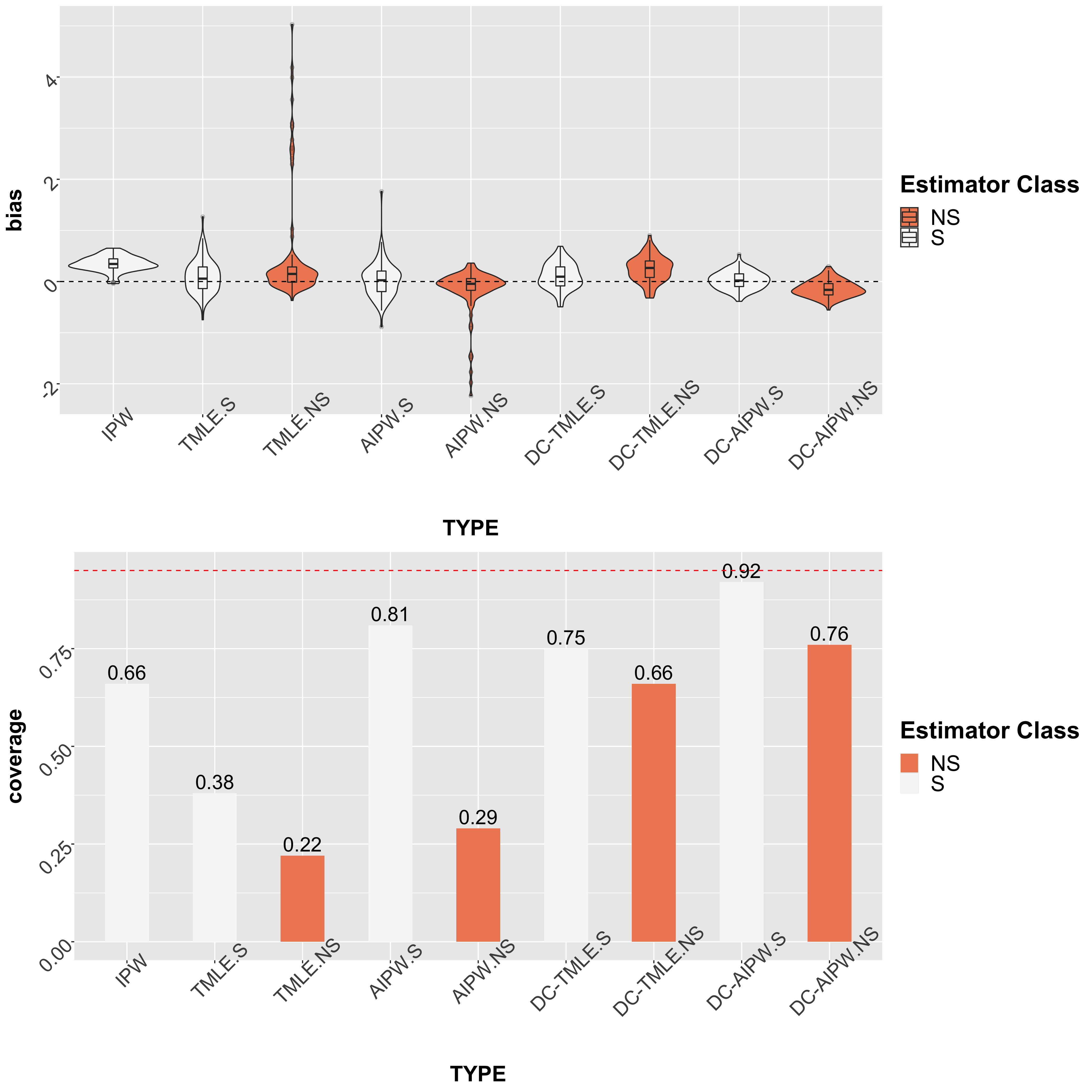
Figure 1: Bias and coverage for all estimators in scenario A.no.int

5.1.2 Result on Scenario B

In Scenario B, our true data generating process has fewer variables than our estimation models. Compared to estimators with the correctly specified models, estimators with excess covariates performed slighty worse in terms of coverage, and in the case of non-smooth learners, ATE bias as well (Table 4). Nonetheless, all estimators with smoothly estimated nuisance functions had similarly low bias and reasonable standard error estimates, with crossfit versions having >95% coverage when excess covariates were included. IPW and non-smoothly estimated TMLE exhibited the worst bias. IPW reached 98% coverage at the cost of overly large SEs and thus wide confidence intervals. In doubly-crossfit models, non-smooth learners were able to produce similar bias and SE estimates as their smooth counterparts.

Table 4: Scenario B: Result from Plasmode simulation on bias, mean squared error (MSE) and 95% confidence interval (CI) coverage. (N = 1178).

	IPW	TMLE		AIPW		DC-TMLE		DC-AIPW
		S	NS	S	NS	S	NS	S	NS
B.cor
Bias ($\times$ 100)	11.72	-0.51	4.53	1.62	-2.63	2.54	-0.97	4.13	-1.38
SE ($\times$ 100)	23.18	12.99	3.97	13.77	3.94	15.71	15.44	16.78	15.86
CI covg.	0.98	0.9	0.41	0.95	0.48	0.96	0.93	0.95	0.97
MSE	0.03	0.03	0.2	0.03	0.02	0.02	0.02	0.03	0.02
BVar	0.02	0.03	0.19	0.03	0.02	0.02	0.02	0.03	0.02
B
Bias ($\times$ 100)	11.89	0.31	9.35	-0.66	-4.95	2.63	2.34	2.51	-7.78
SE ($\times$ 100)	24.78	12.08	3.9	13.32	3.86	15.31	15.99	16.18	15.8
CI covg.	0.99	0.8	0.38	0.92	0.45	0.95	0.97	0.96	0.94
MSE	0.03	0.03	0.53	0.03	0.02	0.02	0.02	0.02	0.03
BVar	0.02	0.03	0.45	0.03	0.01	0.02	0.02	0.02	0.02

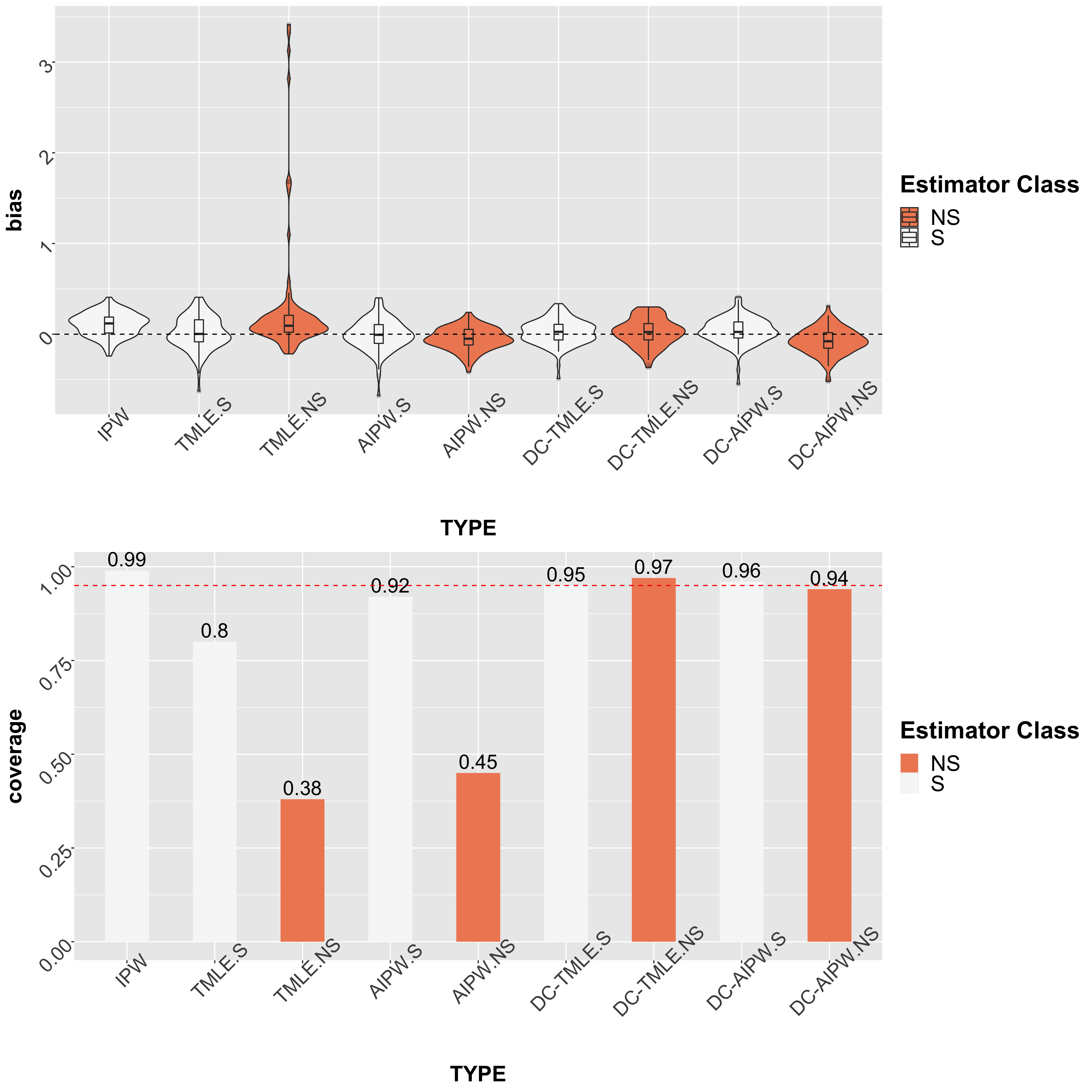
Figure 2: Bias for all 3 cases in scenario B.

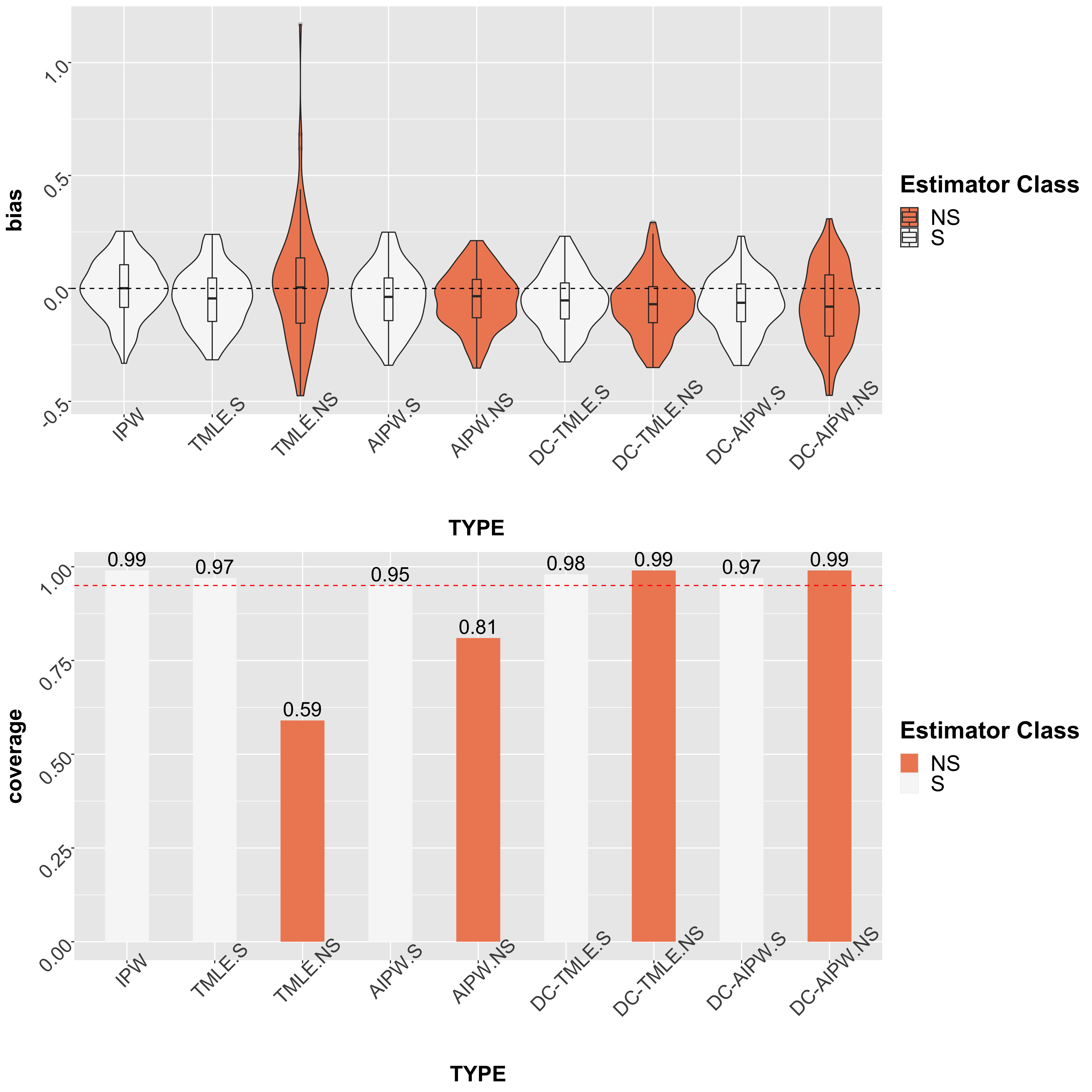
Figure 3: Bias for all 3 cases in scenario C.bad

5.1.3 Result on Scenario C

Table 5: Scenario C: Result from Plasmode simulation on bias, mean squared error (MSE) and 95% confidence interval (CI) coverage.

	TMLE		AIPW		DC-TMLE		DC-AIPW
	S	NS	S	NS	S	NS	S	NS
C.bad
Bias ($\times$ 100)	-4.43	0.45	-3.75	-3.46	-5.31	-6.99	-6.36	-8.06
SE ($\times$ 100)	13.44	8.34	13.52	8.27	15.41	20.76	16.29	21.83
CI covg.	0.97	0.59	0.95	0.81	0.98	0.99	0.97	0.99
MSE	0.02	0.06	0.02	0.02	0.02	0.02	0.02	0.03
BVar	0.02	0.06	0.02	0.02	0.02	0.02	0.02	0.03
C.part
Bias ($\times$ 100)	-2.76	4.12	-2.53	1.2	-4.28	-2.5	-3.74	-5.88
SE ($\times$ 100)	12.72	5.77	12.86	5.77	16.51	22.51	17.43	23.97
CI covg.	0.93	0.45	0.96	0.63	0.98	1	0.99	0.99
MSE	0.02	0.13	0.02	0.02	0.02	0.02	0.02	0.04
BVar	0.02	0.12	0.02	0.02	0.01	0.02	0.02	0.03
C.cor
Bias ($\times$ 100)	0.25	0.87	-0.54	-1.45	-2.65	-3.39	-2.71	-0.41
SE ($\times$ 100)	11.36	4.77	11.34	4.81	12.8	17.69	13.07	22.39
CI covg.	0.94	0.38	0.93	0.49	0.97	1	0.97	0.98
MSE	0.02	0.08	0.02	0.02	0.01	0.02	0.02	0.03
BVar	0.02	0.08	0.02	0.02	0.01	0.01	0.02	0.03

In scenario C, we fit estimators omitting some or all true interactions (effect measure modifiers) between treatment and five key covariates. Unlike other scenarios, the PS model is correctly specified for every estimator. We find that generally, most estimators performed similarly well ( 1-2% bias) with only non-smooth learner estimated, non-crossfit TMLE and AIPW have higher bias (5-6%) and poor coverage (between 38% and 75%). Smooth learner estimated, non-crossfit TMLE and AIPW had nominal coverage, whereas double-crossfit smooth and non-smooth models were overly conservative (coverage 96% to 100%).

5.2 Timing of algorithms

In this section, we present the median real time taken for 100 bootstrap samples of each estimator computed on a Lenovo SD650 NeXtScale server using an Intel 8268 “Cascade Lake”processor and 192GB RAM (table 6). As expected, simple IPW estimators take a negligible amount of time to fit. Estimators fit with non-smooth learners were took 2-3 times as long as their smooth counterparts. Crossfit efficient estimators take proportionally more time than their singly fit counterparts, between 3-6 times longer, due to multiple calls to SuperLearner and additional bootstrapping. While it would be possible to parallelize the crossfitting, the computation time for dependent calls to SuperLeaner within each step would not be able to be reduced.

Table 6: Timing of each algorithm in seconds.

	IPW	TMLE		AIPW		DC-TMLE		DC-AIPW
		Par	Non-Par	Par	Non-Par	Par	Non-Par	Par	Non-Par
A.cor	0.12	20.82	55.86	27.17	63.99	117.47	204.21	120.76	210.24
A.less.1st	0.12	10.13	26.2	13.56	35.95	55.01	149.86	54.68	146.55
A.no.int	0.11	21.49	55.58	21.4	55.69	121.29	203.76	122.34	209.85
C.bad	0.09	3.24	11.01	5.05	27.97	18.39	72.53	17.77	71.81
C.part	0.09	8.67	26.74	12.01	84.82	49.01	125.35	48.8	124.95
C.cor	0.12	3.45	11.17	12.34	89.81	18.34	72.33	18.05	69.91

6 Discussion

6.1 Review of the Findings

Doubly-robust efficient estimators such as AIPW and TMLE represent a state-of-the-art in model-based estimation of causal effects with non-randomized data. Past evaluations of such estimators have been conducted under simpler, more ideal settings e.g. low dimensionality, large sample size, appropriate covariate sets (i.e. no near-instruments), and correct model specification. As highlighted by Balzer and Westling (2021) evaluation of performance will need to be conducted in each setting they are to be applied. Here, we aimed to investigate some more challenging conditions commonly faced by clinical investigators particularly in molecular epidemiology, namely large covariate sets including the potential for weakly-correlated elements or near-instruments, small sample sizes, and substantial nuisance model misspecifiation. We find in our set-up case mirroring the data generating process posed by Kang et al. (2007), double-crossfit estimators fit with non-smooth models performed optimally, but notably there was only a drop in performance on bias and coverage by several percent with smooth models and, as expected, only poor estimation of standard errors without cross-fitting for non-smooth models. In contrast, performance in sets simulated from real data showed much poorer performance even in cases where models were correctly specified. However, in nearly every case double-crossfit AIPW/TMLE fit with smooth models were optimal amongst tested algorithms, even when smooth and non-smooth learners were combined in the SuperLearner.

In scenario A, we presented two forms of model misspecification: first, we completely omitted relevant confounders in both treatment and outcome models (A.less.1st); second, we included all covariates but failed to specify interactions among them (A.no.int). We found all models were suboptimal in parameter and variance estimation, even in the correctly specified case. However, both non-crossfit and doubly crossfit AIPW was the closest to unbiased and nominal coverage, reproducing the result of Naimi et al. (2021) in the crossfit case. In general, we found that all estimators performed poorly when covariates were omitted (A.less.1st) and less poorly when only covariate-interactions were misspecified. This is likely due to the relatively small contribution of interactions to each nuisance model, but also reflects the ability of SuperLearner to some recover some model misspecification thanks to data-adaptive algorithms. More importantly, however, the smoothly fit estimators performed better than their non-smoothly fit counterparts.

In Scenario B, we test a scenario that has not previously been evaluated with respect to these estimators, but is very common in practice – namely when models are fit with an excess of variables which are not part of the true data generating process, but which may be correlated to treatment (instrument), outcome, or both by chance. Mathematically, this over-identification should be irrelevant if all true predictors are included, but the presence of slight misspecification of either model may lead to biased estimates Chatton et al. (2020), notably if chance near-instruments are included in propensity score models Stokes et al. (2020) or non-smooth classifiers overfit either model (Balzer and Westling (2021),Bahamyirou et al. (2019)). On the other hand, penalized regression such as the LASSO are particularly suited to eliminate weakly correlated predictors. In fact, we find a conventionally fit IPW to be biased and over-cover (1.8%; 99% coverage) supporting the substantial literature on bias due to overfit propensity scores. Surprisingly however, doubly-robust estimators fit with non-smooth estimators were also biased and undercover in this scenario (TMLE 1.4% bias; 38% coverage) despite having only true confounders or random variables in models. Smooth TMLE and AIPW were nearly unbiased (<0.1%) with double-crossfit counterparts having nominal coverage at the cost of some slight additional bias ( 0.4%). This suggests all estimators may be quite sensitive to even mild model mis-specifications, in particular, non-smooth-based estimators.

In scenario C, we test the sensitivity of estimators to mis-specification of covariate-treatment interactions, as would be relevant to estimate a population-specific average causal effect (Conzuelo-Rodriguez et al. (2021)). In general, we find that most estimators are in fact relatively unbiased related to other scenarios. However, double-crossfit standard errors were excessively conservative (96% to 100%). Interestingly singly-fit TMLE and AIPW appeared to have lowest bias and nominal coverage across all scenarios while, as expected, the same estimators fit with non-smooth learners had generally poorer performance. Notably, there did not appear to be substantial difference in performance across the scenarios. This may be attributed to the fact that propensity score models were corrected specified in every scenario, highlighting the importance to evaluate realistic scenarios where both models are misspecified.

Overall, we found bias and coverage to be worse across our scenarios and estimators than most past studies, which we attribute mainly to the simulation conditions. Scenarios B and C present estimation problems that are slightly different than past studies, but the relative performance of estimators are reasonably consistent throughout all three scenarios. It is worth highlighting that the fact that bias arises from the chance inclusion of near-instruments further reinforces the need for not only the careful selection of covariates (Chatton et al. (2020)) regardless of the inclusion of penalization algorithms, but also more robust simulation of data congenial to the estimation task faced by the analyst as highlighted by many (Boulesteix et al. (2017), Morris et al. (2019), Stokes et al. (2020), Balzer and Westling (2021)). This work is mostly closely related to Bahamyirou et al. (2019) which employed a Bootstrap Diagnostic Test similar in spirit to plasmode simulation (taking the observed treatment coefficient, rather than setting its value) and Pang et al. (2016b) which employed plasmode simulation. However, in the previous cases, larger sample sizes were employed, fewer covariates (in the case of Bahamyirou, et al), and less severe misspecification. Newer doubly-crossfit estimators were also not employed. In every case, including more recent comparisons (Naimi et al. (2021),Zivich and Breskin (2021)), extent of bias and poor variance estimation appeared to be correctable by improved model specification, hyperparameter tuning, and crossfitting. Benkeser et al. (2017) and Balzer and Westling (2021) show that these challenges occur with simple data generating processes in smaller samples (N < 500), but we show them to persist even in larger datasets (N > 1000). More importantly, we show that challenges in more realistic data sets are difficult to overcome even with correctly specified models. However, in typical clinical or molecular epidemiologic applications, double-crossfit models fit with smooth learners may lead to best parameter and variance estimation among possible options.

6.2 Limitations

First, although with Plasmode we are able to retain correlation among other covariates, the treatment distribution (PS) and the outcome model are still parametrically specified. Thus, there is a major concern that models closer to the data generating process are unfairly favored, potentially explaining the slightly better performance of smoothly-fitted AIPW, as highlighted by Naimi et al. (2021), which directly employs the linear g-computation estimate rather than the scaled logistic estimator. To address this, we also omitted from comparisons the parametric g-computation results which are identical to the plasmode simulation process. The dilemma between simulating with a user specified true parameter and retaining real world data structure remains a natural challenge on simulation method design and is a subject for future development. Second, there are other important features of data generating processes and estimation strategies that we were not able to test for this study. Notably, while we allowed irrelevant covariates to be included in Scenario B, we did not specifically introduce the effects of strong or near-instruments in models, a challenge which has been demonstrated in other contexts (Stokes et al. (2020)). We also did not introduce large libraries or consider extensive hyperparameter tuning as a) this would have substantially contributed to computation time, but more importantly b) we wanted to demonstrate the performance under realistic conditions where the typical clinical science analyst will not spend excessive time on model tuning.

6.3 REFINE2 Tool

What is it? In this study, we found relative performance of efficient estimators to differ substantially from previous simulation studies and we attribute this to the structure of our specific molecular epidemiologic data at hand. As noted previously Balzer and Westling (2021) it is unlikely that universal recommendations can be made as to which estimators will best balance efficiency and robustness to finite-sample properties in every instance. Instead, estimators should be tested against the analyst’s specific data and estimation goals. To this end, we developed the Realistic Evaluations of Finite sample INference using Efficient Estimators (REFINE2) application which enables analysts to reproduce our evaluation pipeline on their own data: namely, easily input their data, generate plasmode simulations of known structure and effect size, and compare the performance of different estimators and algorithm libraries in line with the simulations we presented in this paper. The user-friendly Shiny application can be downloaded free at (https://github.com/mengeks/drml-plasmode, Meng and Huang (2022)) and run offline. All that is required is freely-available R software and the Shiny package. An example dataset and models are included, but users can and should load their own datasets.

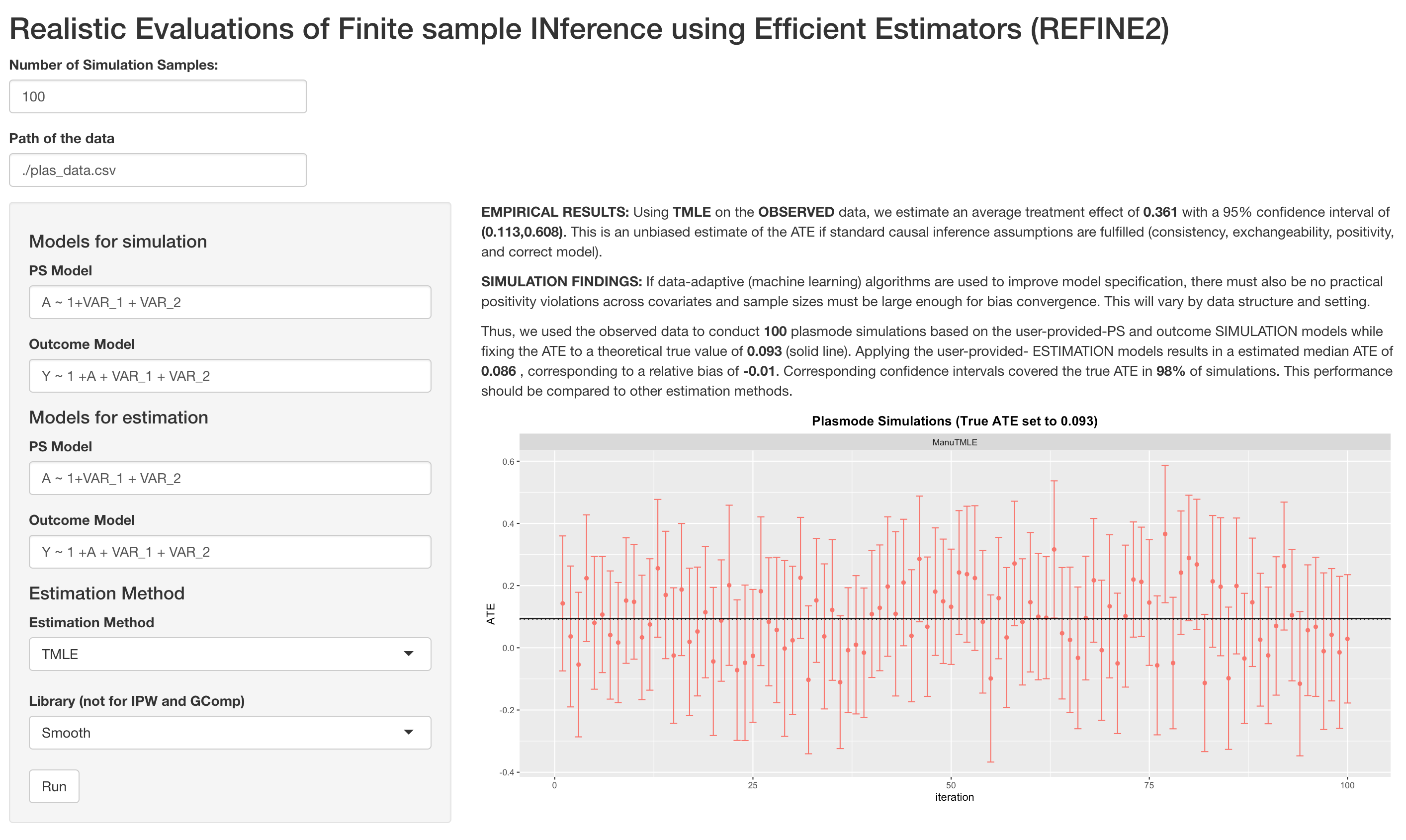
Figure 4: REFINE2: Realistic Evaluations of Finite sample INference using Efficient Estimators

What does it do? The REFINE2 tool allows the analyst to check whether the chosen effect estimation strategy, with or without the use of machine learning algorithms, will reliably estimate an unbiased average treatment effect (ATE) and appropriate confidence intervals given their specific dataset and user-provided parameters. Namely, the user provides:

• the dataset

• number of simulation draws

• Simulation models representing the "true" relationships between treatment, outcome, and covariates (in R syntax)

• Estimation models representing how the effect would be estimated

• chosen estimator (e.g. IPW, DC-TMLE)

• library used to fit the estimator (smooth, non-smooth)

Allowing the user to specify both Simulation and Estimator models ensures maximum flexibility on degree of misspecification. For example, variables could be used to simulate the truth but be omitted or mismeasured in the estimation model to test sensitivity. Using the exact same Simulation and Estimation models will test the finite sample / bias convergence properties of the algorithms on the dataset at hand.

Interpreting output The tool provides several useful outputs. First, without conducting any simulations, REFINE2 provides a fit of the Estimation model using the specified estimator and alogorithms on the observed data to computes the empirical ATE assuming the required causal identification and estimation assumptions are fulfilled. This is useful for analysts who just want to deploy the algorithms.
Second, REFINE2 simulates the specified number of datasets using the Simulation models provided while fixing the true ATE. To reduce the similarity between simulation and estimation models noted above, we use a naive estimator (Y   X) to choose a reasonable true ATE. Next, REFINE2 fits the Estimation models using the chosen estimator and algorithms on each of the simulated steps and reports summary performance measures. This can be then be repeated and compared across different combinations of estimators and algorithms. The simulated data will be stable for any given dataset and set of Simulation models.

Future versions and updates The current version of REFINE2 supports estimation of ATEs using the estimators and learning libraries implemented in this study. Future updates will include additional estimators, customizable SuperLearner libraries, additional estimands (e.g. risk / rate ratios), data generating approaches, and imputation approaches for missing data.

6.4 Conclusions

Our results reinforce the growing call for more thorough evaluation of estimators (Boulesteix et al. (2017)), particularly in settings close to those where they will be deployed Balzer and Westling (2021). Uncommonly considered characteristics such as preservation of observed total treatment and outcome variation from the source data Stokes et al. (2020) can be better assured when only simulating parts of the data generating process and drawing the rest of the covariance matrix as observed. As suggested by Bahamyirou et al. (2019), these simulation approaches can be used more routinely to understand the performance of the estimator for the given analytic context. From our initial establishing simulation, we suggest that past evaluations of these estimators, while demonstrating the potential benefit of doubly-crossfit efficient estimators, did not present sufficiently challenging conditions: differences in performance were less than 10 percent (for both bias and variance), consistent with past studies. However, when we evaluate estimators on sets simulated from real data, drops in performance were much more dramatic, particularly with respect to confidence interval coverage. In such settings, we find across numerous scenarios that crossfit efficient estimators fit with smooth models tend to be the optimal compromise – in the settings where more flexible estimators show a mild benefit, they also have conservative variance estimates at the additional cost of excessive computation time. In settings where numerous effect estimates are desired, such as in bioinformatics, molecular epidemiology, and clinical real-world evidence studies this may be prohibitive. Moreover, we found that even when joining smooth with non-smooth estimators, performance tended to be worse then when only smooth learners were used, a result hinted by Balzer and Westling (2021). Consequently, as Balzer and Westling (2021) we recommend both routine adoption of real-data-based simulation to evaluate estimator performance, and potentially blinded simulation as recommended by Boulesteix et al. (2017), as well as first considering simpler, stable, smooth models for nuisance function in crossfit estimators for typical clinical studies.

Appendix: Exploratory Analysis of the Dataset

We present the histogram of $\binom{331}{2}=54615$ pairs of correlation in Figure 5. Among them, $30$ of these pairs have absolute value greater than $0.7$, $13$ pairs greater than $0.8$, $4$ pairs greater than $0.9$.

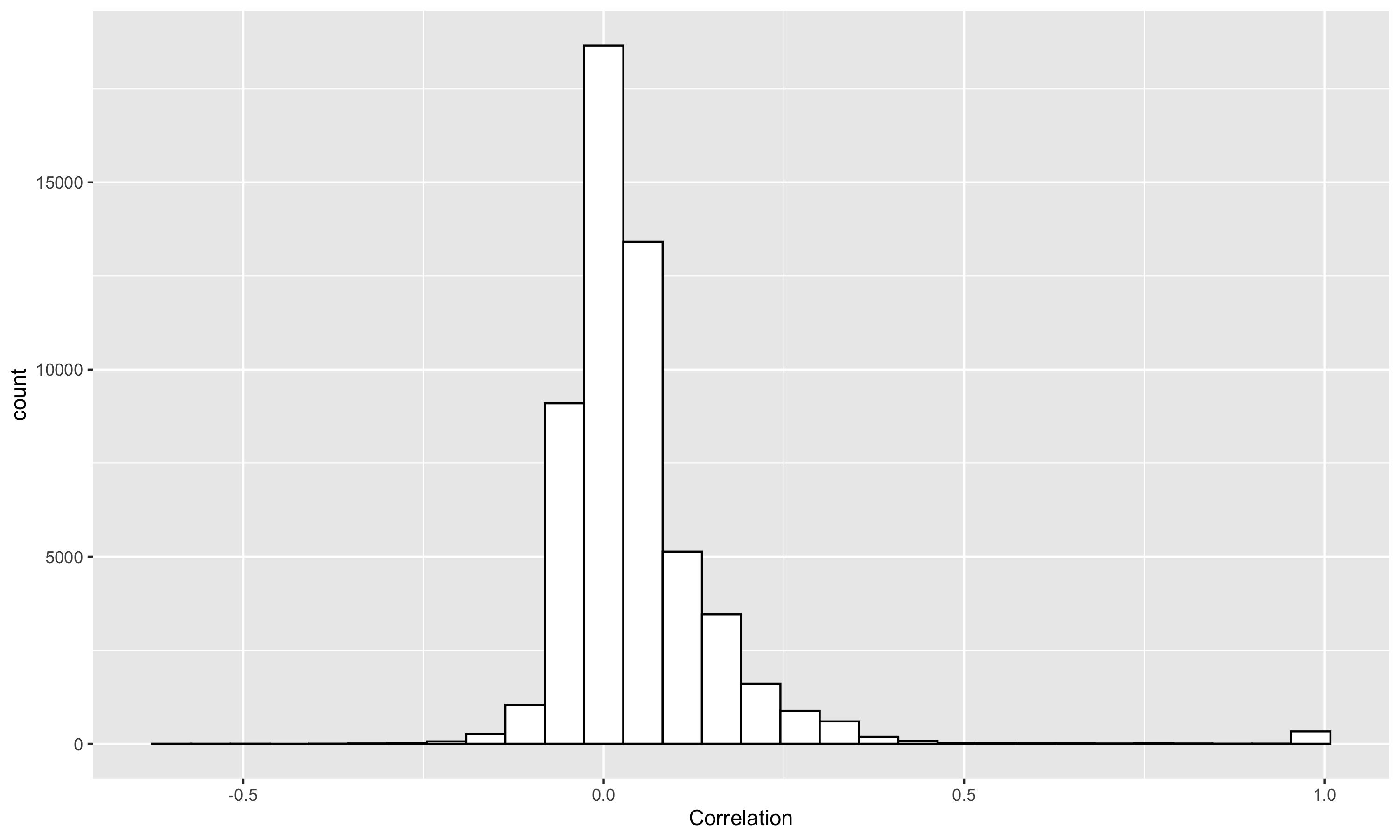
Figure 5: Histogram for Pairwise Correlations

Appendix: Result When Different Number of Double Crossfit Procedures are Used

Increasing the number of double-crossfit procedures (num_cf) (Table 7) from 5 to 10 or 20 did not substantially change the relative performance of any of the estimators, though of course increasing run time proportionally. Hence we decided to proceed with num_cf=5 for all scenarios.

Table 7: Comparison of performance and run time by number of double-crossfitting procedures.

	DC-TMLE		DC-AIPW
	S	NS	S	NS
num_cf=5
Bias ($\times$ 100)	10.96	28.49	1.91	-14.71
SE	0.17	0.16	0.15	0.12
CI covg.	0.76	0.55	0.89	0.73
BVar	0.06	0.09	0.03	0.03
Time	120.09	203.85	119.65	210.38
num_cf=10
Bias ($\times$ 100)	11.1	21.99	0.23	-15.08
SE	0.17	0.19	0.15	0.12
CI covg.	0.83	0.7	0.92	0.76
BVar	0.05	0.06	0.03	0.03
Time	239.58	405.42	237.02	419.68
num_cf=20
Bias ($\times$ 100)	7.83	25.85	-0.03	-15.69
SE	0.18	0.19	0.15	0.13
CI covg.	0.81	0.66	0.91	0.72
BVar	0.05	0.06	0.03	0.03
Time	477.01	810.81	471.6	838.44

Appendix: True Coefficients Used in Plasmode

In generating outcome (OM), there is a term specifying coefficient of exposure variable to 6.6. We present the rest coefficients in the table below. VAR_i corresponds to $X_{i}$ for all i=1,2,…

Table 8: Scenario A: A.cor uses all variables in OM and PS; A.no.int does not have the interaction terms, i.e., lower 10 terms in OM and PS; A.less.1st only includes $(VAR\_1+VAR\_2+VAR\_5+VAR\_18+VAR\_217)^{2}$ and VAR_i, $i\in\{4,7,9,16,17,27,28,31,34,39\}$

	OM Coef	PS Coef
(Intercept)	-3.66	-0.29
VAR_1	0.83	-0.61
VAR_2	0.03	0.24
VAR_5	0.10	0.06
VAR_18	0.15	0.11
VAR_217	0.29	-1.63
VAR_3	-0.03	-0.09
VAR_4	-0.00	0.04
VAR_6	-0.12	-0.42
VAR_7	0.01	0.17
VAR_8	0.02	-0.06
VAR_9	0.38	0.07
VAR_10	0.02	0.22
VAR_11	-0.01	-0.16
VAR_12	0.00	0.21
VAR_13	0.07	0.20
VAR_14	0.03	0.16
VAR_15	-0.00	-0.35
VAR_16	0.34	0.07
VAR_17	0.05	0.17
VAR_19	-0.01	0.30
VAR_20	0.01	-0.07
VAR_21	0.00	0.03
VAR_22	0.01	0.09
VAR_23	-0.00	-0.08
VAR_24	-0.00	-0.16
VAR_25	0.02	0.15
VAR_26	-0.01	-0.00
VAR_27	0.00	0.00
VAR_28	-0.01	-0.01
VAR_29	-0.00	0.01
VAR_30	-0.03	-0.59
VAR_31	0.00	0.00
VAR_32	0.06	0.27
VAR_33	0.04	-0.62
VAR_34	0.00	-0.01
VAR_35	0.01	0.16
VAR_36	0.00	-0.00
VAR_37	0.06	0.08
VAR_38	-0.00	0.00
VAR_39	-0.09	0.11
VAR_40	0.52	-0.53
VAR_1:VAR_2	-0.01	0.01
VAR_1:VAR_5	-0.18	0.08
VAR_1:VAR_18	-0.17	-0.13
VAR_1:VAR_217	0.03	0.64
VAR_2:VAR_5	0.04	0.14
VAR_2:VAR_18	-0.02	-0.19
VAR_2:VAR_217	0.03	-0.00
VAR_5:VAR_18	0.04	0.18
VAR_5:VAR_217	-0.06	0.35
VAR_18:VAR_217	0.00	-0.02

Figure 6: Plot for Parameters in Scenario. Fixed means those in all 3 simulations, i.e., first order terms for variable 1, 2,5,18,217;1st means all other first order terms in variables 1 to 40; int means interaction terms among variables 1, 2,5,18,217

Table 9: Scenario B coefficients

	OM Coef	PS Coef
(Intercept)	-3.77	-10.35
VAR_1	0.89	0.22
VAR_2	0.13	0.67
VAR_5	0.06	0.45
VAR_18	0.21	0.62
VAR_217	0.29	-1.77
VAR_34	0.00	-0.00
VAR_27	-0.00	-0.00
VAR_4	-0.01	-0.02
VAR_31	-0.00	-0.00
VAR_28	-0.01	0.00
VAR_17	0.05	0.21
VAR_16	0.34	0.09
VAR_9	0.50	0.68
VAR_7	0.05	0.04
VAR_39	-0.09	-0.01
VAR_1:VAR_2	-0.03	-0.10
VAR_1:VAR_5	-0.19	-0.10
VAR_1:VAR_18	-0.17	-0.03
VAR_1:VAR_217	0.04	0.45
VAR_2:VAR_5	0.04	0.11
VAR_2:VAR_18	-0.01	0.02
VAR_2:VAR_217	0.01	0.12
VAR_5:VAR_18	0.02	-0.13
VAR_5:VAR_217	-0.05	0.43
VAR_18:VAR_217	0.01	0.02

Table 10: Scenario C Coefficients

	OM Coef	PS Coef
(Intercept)	12.49	-4.86
VAR_1	1.16	0.38
VAR_2	-0.37	0.63
VAR_5	-0.19	0.64
VAR_18	-0.01	0.45
VAR_217	0.64	-1.64
A1:VAR_1	-1.37	0.00
A1:VAR_2	0.41	0.00
A1:VAR_5	-1.89	0.00
A1:VAR_18	0.04	0.00
A1:VAR_217	1.24	0.00
VAR_1:VAR_2	-0.08	-0.13
VAR_1:VAR_5	-0.26	-0.18
VAR_1:VAR_18	-0.19	-0.03
VAR_1:VAR_217	0.02	0.45
VAR_2:VAR_5	0.27	0.14
VAR_2:VAR_18	-0.00	0.03
VAR_2:VAR_217	0.03	0.12
VAR_5:VAR_18	0.11	-0.06
VAR_5:VAR_217	-0.17	0.37
VAR_18:VAR_217	0.08	0.03

References

- Bahamyirou et al. (2019) Asma Bahamyirou, Lucie Blais, Amélie Forget, and Mireille E Schnitzer. Understanding and diagnosing the potential for bias when using machine learning methods with doubly robust causal estimators. Statistical methods in medical research, 28(6):1637–1650, 2019.
- Balzer and Westling (2021) Laura B Balzer and Ted Westling. Demystifying statistical inference when using maching learning in causal research. American Journal of Epidemiology, 2021.
- Balzer et al. (2016) Laura B Balzer, Mark J van der Laan, Maya L Petersen, and SEARCH Collaboration. Adaptive pre-specification in randomized trials with and without pair-matching. Stat. Med., 35(25):4528–4545, November 2016.
- Benkeser et al. (2017) David Benkeser, Marco Carone, MJ Van Der Laan, and PB Gilbert. Doubly robust nonparametric inference on the average treatment effect. Biometrika, 104(4):863–880, 2017.
- Benkeser et al. (2020) David Benkeser, Weixin Cai, Mark J van der Laan, et al. A nonparametric super-efficient estimator of the average treatment effect. Statistical Science, 35(3):484–495, 2020.
- Boulesteix et al. (2017) Anne-Laure Boulesteix, Rory Wilson, and Alexander Hapfelmeier. Towards evidence-based computational statistics: lessons from clinical research on the role and design of real-data benchmark studies. BMC Medical Research Methodology, 17(1):1–12, 2017.
- Challa et al. (2020) Anup P. Challa, Robert R. Lavieri, Ethan S. Lippmann, Jeffery A. Goldstein, Lisa Bastarache, Jill M. Pulley, and David M. Aronoff. EHRs could clarify drug safety in pregnant people. Nature Medicine, 26(6):820–821, May 2020. doi: 10.1038/s41591-020-0925-1. URL https://doi.org/10.1038/s41591-020-0925-1.
- Chatton et al. (2020) Arthur Chatton, Florent Le Borgne, Clémence Leyrat, Florence Gillaizeau, Chloé Rousseau, Laetitia Barbin, David Laplaud, Maxime Léger, Bruno Giraudeau, and Yohann Foucher. G-computation, propensity score-based methods, and targeted maximum likelihood estimator for causal inference with different covariates sets: a comparative simulation study. Scientific Reports, 10:9219, 2020.
- Chernozhukov et al. (2018) Victor Chernozhukov, Denis Chetverikov, Mert Demirer, Esther Duflo, Christian Hansen, Whitney Newey, and James Robins. Double/debiased machine learning for treatment and structural parameters, 2018.
- Conzuelo-Rodriguez et al. (2021) Gabriel Conzuelo-Rodriguez, Lisa M Bodnar, Maria M Brooks, Abdus Wahed, Edward H Kennedy, Enrique Schisterman, and Ashley I Naimi. Performance evaluation of parametric and nonparametric methods when assessing effect measure modification. American Journal of Epidemiology, 2021.
- Díaz (2020) Iván Díaz. Machine learning in the estimation of causal effects: targeted minimum loss-based estimation and double/debiased machine learning. Biostatistics, 21(2):353–358, April 2020.
- Díaz and van der Laan (2017) Iván Díaz and Mark J van der Laan. Doubly robust inference for targeted minimum loss-based estimation in randomized trials with missing outcome data. Stat. Med., 36(24):3807–3819, October 2017.
- Dickerman et al. (2019) Barbra A. Dickerman, Xabier García-Albéniz, Roger W. Logan, Spiros Denaxas, and Miguel A. Hernán. Avoidable flaws in observational analyses: an application to statins and cancer. Nature Medicine, 25(10):1601–1606, October 2019. doi: 10.1038/s41591-019-0597-x. URL https://doi.org/10.1038/s41591-019-0597-x.
- Franklin et al. (2014) Jessica M Franklin, Sebastian Schneeweiss, Jennifer M Polinski, and Jeremy A Rassen. Plasmode simulation for the evaluation of pharmacoepidemiologic methods in complex healthcare databases. Computational statistics & data analysis, 72:219–226, 2014.
- Funk et al. (2011) Michele Jonsson Funk, Daniel Westreich, Chris Wiesen, Til Stürmer, M Alan Brookhart, and Marie Davidian. Doubly robust estimation of causal effects. American journal of epidemiology, 173(7):761–767, 2011.
- Gruber and van der Laan (2010) Susan Gruber and Mark J van der Laan. An application of collaborative targeted maximum likelihood estimation in causal inference and genomics. Int. J. Biostat., 6(1):Article 18, May 2010.
- Hill et al. (2016) Steven M Hill, Laura M Heiser, Thomas Cokelaer, Michael Unger, Nicole K Nesser, Daniel E Carlin, Yang Zhang, Artem Sokolov, Evan O Paull, Chris K Wong, Kiley Graim, Adrian Bivol, Haizhou Wang, Fan Zhu, Bahman Afsari, Ludmila V Danilova, Alexander V Favorov, Wai Shing Lee, Dane Taylor, Chenyue W Hu, Byron L Long, David P Noren, Alexander J Bisberg, HPN-DREAM Consortium, Gordon B Mills, Joe W Gray, Michael Kellen, Thea Norman, Stephen Friend, Amina A Qutub, Elana J Fertig, Yuanfang Guan, Mingzhou Song, Joshua M Stuart, Paul T Spellman, Heinz Koeppl, Gustavo Stolovitzky, Julio Saez-Rodriguez, and Sach Mukherjee. Inferring causal molecular networks: empirical assessment through a community-based effort. Nat. Methods, 13(4):310–318, April 2016.
- Horvitz and Thompson (1952) Daniel G Horvitz and Donovan J Thompson. A generalization of sampling without replacement from a finite universe. Journal of the American statistical Association, 47(260):663–685, 1952.
- Huang et al. (2021) Jonathan Yinhao Huang, Shirong Cai, Zhongwei Huang, Mya Thway Tint, Wen Lun Yuan, Izzuddin M Aris, Keith M Godfrey, Neerja Karnani, Yung Seng Lee, Jerry Kok Yen Chan, Yap Seng Chong, Johan Gunnar Eriksson, and Shiao-Yng Chan. Analyses of child cardiometabolic phenotype following assisted reproductive technologies using a pragmatic trial emulation approach. Nat. Commun., 12(1):5613, September 2021.
- Ju et al. (2019) Cheng Ju, Susan Gruber, Samuel D Lendle, Antoine Chambaz, Jessica M Franklin, Richard Wyss, Sebastian Schneeweiss, and Mark J van der Laan. Scalable collaborative targeted learning for high-dimensional data. Stat. Methods Med. Res., 28(2):532–554, February 2019.
- Kang et al. (2007) Joseph DY Kang, Joseph L Schafer, et al. Demystifying double robustness: A comparison of alternative strategies for estimating a population mean from incomplete data. Statistical science, 22(4):523–539, 2007.
- Koch et al. (2017) Brandon Koch Koch, David M Vock, and Julian Wolfson. Covariate selection with group lasso and doubly robust estimation of causal effects. Biometrics, 74(1):8–17, 2017.
- Koehler et al. (2009) Elizabeth Koehler, Elizabeth Brown, and Sebastien J-PA Haneuse. On the assessment of monte carlo error in simulation-based statistical analyses. The American Statistician, 63(2):155–162, 2009.
- Kreif et al. (2017) Noémi Kreif, Linh Tran, Richard Grieve, Bianca De Stavola, Robert C Tasker, and Maya Petersen. Estimating the comparative effectiveness of feeding interventions in the pediatric intensive care unit: A demonstration of longitudinal targeted maximum likelihood estimation. Am. J. Epidemiol., 186(12):1370–1379, December 2017.
- Larrañaga et al. (2006) Pedro Larrañaga, Borja Calvo, Roberto Santana, Concha Bielza, Josu Galdiano, Iñaki Inza, José A. Lozano, Rubén Armañanzas, Guzmán Santafé, Aritz Pérez, and Victor Robles. Machine learning in bioinformatics. Briefings in Bioinformatics, 7(1):86–112, 03 2006. ISSN 1467-5463. doi: 10.1093/bib/bbk007. URL https://doi.org/10.1093/bib/bbk007.
- Lecca (2021) Paola Lecca. Machine learning for causal inference in biological networks: Perspectives of this challenge. Frontiers in Bioinformatics, 1, 2021. ISSN 2673-7647. doi: 10.3389/fbinf.2021.746712. URL https://www.frontiersin.org/article/10.3389/fbinf.2021.746712.
- Li et al. (2010) Yang Li, Bruno M. Tesson, Gary A. Churchill, and Ritsert C. Jansen. Critical reasoning on causal inference in genome-wide linkage and association studies. Trends in Genetics, 26(12):493–498, 2010. ISSN 0168-9525. doi: https://doi.org/10.1016/j.tig.2010.09.002. URL https://www.sciencedirect.com/science/article/pii/S0168952510001885.
- Libbrecht and Noble (2015) Maxwell W Libbrecht and William Stafford Noble. Machine learning applications in genetics and genomics. Nat. Rev. Genet., 16(6):321–332, June 2015.
- Lunceford and Davidian (2004) Jared K Lunceford and Marie Davidian. Stratification and weighting via the propensity score in estimation of causal treatment effects: a comparative study. Statistics in medicine, 23(19):2937–2960, 2004.
- Meng and Huang (2022) Xiang Meng and Jon Huang. Code for the paper "refine2: A tool to evaluate real-world performance of machine-learning based effect estimators for molecular and clinical studies", 2022. URL https://zenodo.org/record/4930877.
- Morris et al. (2019) Tim P Morris, Ian R White, and Michael J Crowther. Using simulation studies to evaluate statistical methods. Statistics in medicine, 38(11):2074–2102, 2019.
- Naimi et al. (2021) Ashley I Naimi, Alan E Mishler, and Edward H Kennedy. Challenges in obtaining valid causal effect estimates with machine learning algorithms. American Journal of Epidemiology, 2021.
- Ness et al. (2016) Robert O Ness, Karen Sachs, and Olga Vitek. From correlation to causality: Statistical approaches to learning regulatory relationships in large-scale biomolecular investigations. J. Proteome Res., 15(3):683–690, March 2016.
- Newey and Robins (2018) Whitney K Newey and James R Robins. Cross-fitting and fast remainder rates for semiparametric estimation. arXiv preprint arXiv:1801.09138, 2018.
- Ning et al. (2020) Yang Ning, Peng Sida, and Kosuke Imai. Robust estimation of causal effects via a high-dimensional covariate balancing propensity score. Biometrika, 107(3):533–554, 2020.
- Pang et al. (2016a) Menglan Pang, Tibor Schuster, Kristian B Filion, Mireille E Schnitzer, Maria Eberg, and Robert W Platt. Effect estimation in point-exposure studies with binary outcomes and high-dimensional covariate data - a comparison of targeted maximum likelihood estimation and inverse probability of treatment weighting. Int. J. Biostat., 12(2), November 2016a.
- Pang et al. (2016b) Menglan Pang, Tibor Schuster, Kristian B Filion, Mireille E Schnitzer, Maria Eberg, and Robert W Platt. Effect estimation in point-exposure studies with binary outcomes and high-dimensional covariate data–a comparison of targeted maximum likelihood estimation and inverse probability of treatment weighting. The international journal of biostatistics, 12(2), 2016b.
- Park and Kellis (2021) Yongjin P Park and Manolis Kellis. CoCoA-diff: counterfactual inference for single-cell gene expression analysis. Genome Biol., 22(1):228, August 2021.
- Prosperi et al. (2020) Mattia Prosperi, Yi Guo, Matt Sperrin, James S. Koopman, Jae S. Min, Xing He, Shannan Rich, Mo Wang, Iain E. Buchan, and Jiang Bian. Causal inference and counterfactual prediction in machine learning for actionable healthcare. Nature Machine Intelligence, 2(7):369–375, July 2020. doi: 10.1038/s42256-020-0197-y. URL https://doi.org/10.1038/s42256-020-0197-y.
- Robins et al. (2007) James Robins, Mariela Sued, Quanhong Lei-Gomez, and Andrea Rotnitzky. Comment: Performance of double-robust estimators when "inverse probability" weights are highly variable. Statistical Science, 22(4):544–559, 2007.
- Rosenbaum and Rubin (1983) Paul R Rosenbaum and Donald B Rubin. The central role of the propensity score in observational studies for causal effects. Biometrika, 70(1):41–55, 1983.
- Rossides et al. (2021) Marios Rossides, Susanna Kullberg, Daniela Di Giuseppe, Anders Eklund, Johan Grunewald, Johan Askling, and Elizabeth V Arkema. Infection risk in sarcoidosis patients treated with methotrexate compared to azathioprine: A retrospective ’target trial’ emulated with swedish real-world data. Respirology, 26(5):452–460, May 2021.
- Rotnitzky et al. (2019) Andrea Rotnitzky, Ezequiel Smucler, and James M Robins. Characterization of parameters with a mixed bias property. arXiv preprint arXiv:1904.03725, 2019.
- Schneeweiss et al. (2009) Sebastian Schneeweiss, Jeremy A Rassen, Robert J Glynn, Jerry Avorn, Helen Mogun, and M Alan Brookhart. High-dimensional propensity score adjustment in studies of treatment effects using health care claims data. Epidemiology (Cambridge, Mass.), 20(4):512, 2009.
- Schuler and Rose (2017) Megan S Schuler and Sherri Rose. Targeted maximum likelihood estimation for causal inference in observational studies. American journal of epidemiology, 185(1):65–73, 2017.
- Sofrygin et al. (2019) Oleg Sofrygin, Zheng Zhu, Julie A Schmittdiel, Alyce S Adams, Richard W Grant, Mark J van der Laan, and Romain Neugebauer. Targeted learning with daily EHR data. Stat. Med., 38(16):3073–3090, July 2019.
- Soh et al. (2014) SE Soh, MT Tint, PD Gluckman, KM Godfrey, A Rifkin-Graboi, YH Chan, W Stünkel, JD Holbrook, K Kwek, YS Chong, and SM; GUSTO Study Group Saw. Cohort profile: Growing up in singapore towards healthy outcomes (gusto) birth cohort study. Int J Epidemiol, 43(5):1401–1409, 2014.
- Stokes et al. (2020) Tyrel Stokes, Russell Steele, and Ian Shrier. Causal simulation experiments: Lessons from bias amplification. arXiv preprint arXiv:2003.08449, 2020.
- (49) R Core Team. R model formula. URL https://stat.ethz.ch/R-manual/R-patched/library/stats/html/formula.html.
- van der Laan and Gruber (2010) Mark J van der Laan and Susan Gruber. Collaborative double robust targeted maximum likelihood estimation. The international journal of biostatistics, 6(1), 2010.
- Van der Laan et al. (2007) Mark J Van der Laan, Eric C Polley, and Alan E Hubbard. Super learner. 2007.
- Wang and Wu (2019) May D. Wang and Hang Wu. Tutorial: Causal inference in biomedical data analytics – basics and recent advances. In Proceedings of the 10th ACM International Conference on Bioinformatics, Computational Biology and Health Informatics, BCB ’19, page 558, New York, NY, USA, 2019. Association for Computing Machinery. ISBN 9781450366663. doi: 10.1145/3307339.3343177. URL https://doi.org/10.1145/3307339.3343177.
- White and Vignes (2019) Alex White and Matthieu Vignes. Causal queries from observational data in biological systems via bayesian networks: An empirical study in small networks. Methods Mol. Biol., 1883:111–142, 2019.
- Wyss et al. (2018) Richard Wyss, Sebastian Schneeweiss, Mark Van Der Laan, Samuel D Lendle, Cheng Ju, and Jessica M Franklin. Using super learner prediction modeling to improve high-dimensional propensity score estimation. Epidemiology, 29(1):96–106, 2018.
- Yu et al. (2019) Ya-Hui Yu, Lisa M Bodnar, Maria M Brooks, Katherine P Himes, and Ashley I Naimi. Comparison of parametric and nonparametric estimators for the association between incident prepregnancy obesity and stillbirth in a population-based cohort study. Am. J. Epidemiol., 188(7):1328–1336, July 2019.
- Zivich and Breskin (2021) Paul N Zivich and Alexander Breskin. Machine learning for causal inference: on the use of cross-fit estimators. Epidemiology, 2021.