Causally Constrained Data Synthesis for Private Data Release

Abstract

Making evidence based decisions requires data. However for real-world applications, the privacy of data is critical. Using synthetic data which reflects certain statistical properties of the original data preserves the privacy of the original data. To this end, prior works utilize differentially private data release mechanisms to provide formal privacy guarantees. However, such mechanisms have unacceptable privacy vs. utility trade-offs. We propose incorporating causal information into the training process to favorably modify the aforementioned trade-off. We theoretically prove that generative models trained with additional causal knowledge provide stronger differential privacy guarantees. Empirically, we evaluate our solution comparing different models based on variational auto-encoders (VAEs), and show that causal information improves resilience to membership inference, with improvements in downstream utility.

1 Introduction

Automating AI-based solutions and making evidence-based decisions both require data analyses. However, in many situations, such as healthcare (Jordon et al., 2020) or social justice (Edge et al., 2020), the data is very sensitive and cannot be published directly to protect the privacy of participants involved. Synthetic data generation, which captures certain statistical properties of the original data, is useful to resolve these issues. However, naive data creation may not work; when improperly constructed, the synthetic data can leak information about its sensitive counterpart (from which it was constructed). Several membership and attribute inference attacks have been shown to impact specific subgroups (Mukherjee et al., 2019; Stadler et al., 2020; Zhang et al., 2020b), and eliminate any privacy advantage provided by releasing synthetic data. Therefore, efficient privacy-preserving synthetic data generation methods are needed.

The de-facto mechanism used for providing privacy in synthetic data release is that of differential privacy (Dwork et al., 2006). The privacy vs. utility trade-off inherent with these solutions is further exacerbated in tabular data because of the correlations between different records, and among different attributes within a record as well. In such settings, the amount of noise required to provide meaningful privacy guarantees often destroys any discernible signal. Apart from assumptions made on the independence of records and attributes, prior works make numerous assumptions about the nature of usage of the synthetic dataset (Xiao et al., 2010; Hardt et al., 2010; Cormode et al., 2019; Dwork et al., 2009). This results in heuristic and one-off solutions that do not easily port to different settings.

To this end, we propose a mechanism to create synthetic data that is agnostic to the downstream task. Similar to prior work (Jordon et al., 2018), our solution involves training a generative model to provide formal differential privacy guarantees. Unlike prior solutions, however, we encode domain knowledge into the generation process to enable better utility. In particular, to induce favorable privacy vs. utility trade-offs, our main contribution involves incorporating causal information while training synthetic data generative models. We formally prove that generative models trained with causal knowledge of the specific dataset are more private than their non-causal counterparts. Prior work has shown the privacy benefits of causal learning in only discriminative setting (Tople et al., 2020). In comparison, our result is more generic, and applies across the spectrum (for both discriminative and generative models).

Based on our theoretical results, we present a novel practical solution, utilizing advances in deep generative models, in particular, variations autoencoder (VAE) based models (Kingma & Welling, 2013; Rezende et al., 2014). These models combine the advantage of both deep learning and probabilistic modeling, making them scale to large datasets, flexible to fit complex data in a probabilistic manner, and can be used for data generation (Ma et al., 2019; 2020a). Thus, in designing our solution, we assume structured causal graphs (SCGs) as prior knowledge and train causally consistent VAEs. Additionally, we train causally consistent differentially-private VAEs to understand the benefit of causality in conjunction to that of differential privacy.

We experimentally evaluate our solution for utility and privacy trade-off on two real world applications: (a) a medical dataset regarding neuropathetic pain (Tu et al., 2019b), and (b) a student response dataset from a real-world online education platform (Wang et al., 2020). Based on causal knowledge provided by a domain expert, we show that models that are causally consistent are more stable by design. In the absence of differentially-private noise, causal models elevate the baseline utility by $2.42$ percentage on average while non-causal models degrade it by $3.49$ percentage. Consequently, when provided the same privacy budget, causally consistent models are more utilitarian in downstream tasks than their non-causal counterparts. This demonstrates that causal models allow us to extract more of the utility from the synthetic data while maintaining theoretical privacy guarantees.

With respect to privacy evaluation, prior works solely rely on the value of the privacy budget $\varepsilon$. We take this one step further and empirically evaluate attacks. Our experimental results demonstrate the positive impact of causality in inhibiting the membership inference adversary’s advantage. Better still, we demonstrate that differentially-private models that incorporate both complete or even partial (or incomplete) causal information are more resilient to membership inference adversaries than those with purely differential privacy with the exact same $\varepsilon$-DP guarantees. These results strengthen the need for using empirical attacks as an additional measure to evaluate privacy guarantees of a given private generative model.

In summary, the contributions of our work include:

1. A deeper understanding of the advantages of causality through a theoretical result that highlights the privacy amplification induced by causal consistency (§ 3).

2. An efficient and scalable mechanism for causally-consistent and differentially private data release (§ 4).

3. Empirical results demonstrating that causally constrained (and differentially private) models are more resilient to membership inference as compared to non-causal counterparts, without significant accuracy degradation (§ 6).

2 Problem Statement & Notation

Problem Statement: We study the problem of private data release, where a data owner is in possession of a sensitive dataset which they wish to release. Formally, we define a dataset $D$ to be the set $\{\mathbf{x}_{1},\cdots\mathbf{x}_{n}\}$ of $n$ records, where each record $\mathbf{x}=(x_{1},\cdots,x_{k})$ has $k$ attributes. We refer to $n$ as the dataset size, and $d$ as the dimensionality of the data. Each record $\mathbf{x}$ belongs to the universe of records $\mathcal{X}$.

Our approach involves designing a procedure which takes in a sensitive dataset $D_{p}$ and outputs a synthetic dataset $D_{s}$ which has some formal privacy guarantee and maintains properties from original dataset for downstream decision-making tasks. Formally speaking, we wish to design $f_{\theta}:Z\rightarrow\mathcal{X}$, where $\theta$ are the parameters of the method, and $Z$ is some underlying latent representation for inputs in $\mathcal{X}$.

2.1 Preliminaries

In our work, we wish for $f_{\theta}$ to provide the guarantee of differential privacy. Below, we define useful concepts related to the same.

Differential Privacy  (Dwork et al., 2006):. Let $\varepsilon\in\mathbb{R}^{+}$ be the privacy budget, and $H$ be a randomized mechanism that takes a dataset as input. $H$ is said to provide $\varepsilon$-differential privacy if, for all datasets $D_{1}$ and $D_{2}$ that differ on a single record, and all subsets $S$ of the outcomes of running $H$: $\mathbb{P}[H(D_{1})\in S]\leq e^{\varepsilon}\cdot\mathbb{P}[H(D_{2})\in S]$, where the probability is over the randomness of $H$.

Sensitivity: Let $d\in\mathbb{Z}^{+}$, ${\mathcal{D}}$ be a collection of datasets, and define $H:\mathcal{D}\rightarrow\mathbb{R}^{d}$. The $\ell_{1}$ sensitivity of $H$, denoted $\Delta H$, is defined by $\Delta H=\max\lVert H(D_{1})-H(D_{2})\rVert_{1}$, where the maximum is over all pairs of datasets $D_{1}$ and $D_{2}$ in ${\mathcal{D}}$ differing in at most one record.

We rely on generative models to enable private data release. Formally, if the generative models are trained to provide differential privacy, then any further post-processing (such as using the generative model to obtain a synthetic dataset) is also differentially private by the post-processing property of differential privacy (Dwork et al., 2014).

Causally Consistent Models: Formally, the underlying data generating process (DGP) is characterized by a causal graph that describes the conditional independence relationships between different variables. In this work, we use the term causally consistent models to refer to those models that factorize in the causal direction. For example, the graph $X_{1}\rightarrow X_{2}$ implies that the factorization following the causal direction is $\mathbb{P}(X_{1},X_{2})=\mathbb{P}(X_{1})\cdot\mathbb{P}(X_{2}|X_{1})$.Due to the modularity property (Woodward, 2005), the mechanism to generate $x_{2}$ from $x_{1}$ is independent from the marginal distribution of $x_{1}$. This only holds in causal factorization but not in anti-causal factorization.

3 Privacy Amplification Through Causality

In this section, we present our main result: causally consistent (or causal) models are more private than their non-causal/associational counterparts. Our focus is on generative models, but our analysis is applicable to both generative and discriminative contexts.

3.1 Main Theorem

We begin by introducing notations and definitions needed for our proof. A mechanism $M$ takes in as input a dataset $D$ and outputs a parameterized model $f_{\theta}$. The model output by the mechanism $M$ belongs to a hypothesis space $\mathcal{H}$. The dataset $D$ comprises of samples, where each sample $\mathbf{x}=(x_{1},\cdots,x_{k})$ comprises of $k$ features. To learn the model, we utilize empirical risk mechanism (ERM), and assume a loss function $\mathcal{L}$ that is Lipschitz continuous and strongly convex. $\mathcal{L}_{D}$ denotes the average loss calculated over the dataset $D$ (i.e., $\mathcal{L}_{D}=\frac{1}{n}\sum_{\mathbf{x}\in D}\mathcal{L}_{\mathbf{x}}$). $\mathcal{L}_{\mathbf{x}}$ denotes the loss being calculated over sample $\mathbf{x}$ i.e., $\mathcal{L}_{\mathbf{x}}(f_{\theta})=\mathcal{L}_{\mathbf{x}}(f_{\theta}(\mathbf{x}))$. For generative models, the loss should reflect how well the model fits the data while for probabilistic models, and if we use variational inference, we can not minimize the KL divergence exactly, but one instead minimizes a function that is equal to it up to a constant, which is the evidence lower bound (ELBO).

Data Generating Process (DGP): DGP $<f^{*},\eta>$ is obtained as follows: $f^{*}=\lim_{n\to\infty}\operatorname*{arg\,min}\mathcal{L}_{D}(f_{\theta})$. Essentially $f^{\star}$ can be thought of as the infinite data limit of the ERM learner and can be viewed as the ground truth. In a causal setting, the DGP for a variable $X$ is defined as $f^{*}(X)=(f^{*}_{1}(Pa(X_{1}))+\eta_{i},\cdots,f^{*}_{n}(Pa(X_{n}))+\eta_{n})$ where $\eta_{i}$ are mutually, independently chosen noise and $Pa(X_{i})$ are the parents of $X_{i}$ in the SCG.

Loss-maximizing (LM) Adversary: Given a model $f_{\theta}$ and a loss function $\mathcal{L}$, an LM adversary chooses a point $\mathbf{x}^{\prime}$ (to be added to the dataset $D$ to obtain a neighboring dataset $D^{\prime}$) as $\mathbf{x^{\prime}}=\arg\max_{\mathbf{x}}\mathcal{L}_{\mathbf{x}}(f_{\theta})$.

Empirical Risk Minimization (ERM): For a given hypothesis class $\mathcal{H}$, and a dataset $D$, the ERM learner uses the ERM rule to choose parameters $\theta\in\mathcal{H}$, with the lowest possible error over $D$. Formally, $f_{\theta^{*}}=\operatorname*{arg\,min}_{\theta\in\mathcal{H}}\mathcal{L}_{D}(f_{\theta})$ denotes the optimal model.

Theorem 1.

Given a dataset $D$ of size $n$, and a strongly convex and Lipschitz continuous loss function $\mathcal{L}$, assume we train two models in a differentially private manner: a causal (generative) model $f_{\theta_{c}}$, and an associational (generative) model $f_{\theta_{a}}$, such that they minimize $\mathcal{L}$ on $D$. Assume that the class of hypotheses $\mathcal{H}$ is expressive enough such that the true causal function lies in $\mathcal{H}$.

1. Infinite sample case. As $n\to\infty$, the privacy budget of the causal model is lower than that of the associational model i.e., $\varepsilon_{c}\leq\varepsilon_{a}$.

2. Finite sample case. For finite $n$, assuming certain conditions on the associational models learnt, the privacy budget of the causal model is lower than that of the associational model i.e., $\varepsilon_{c}\leq\varepsilon_{a}$.

Proof Outline: The detailed proof is found in Appendix A. The main steps of our proof are as follows:

1. We show that the maximum loss of a causal model is lower than or equal to maximum loss of the corresponding associational model.

2. Using strong convexity and Lipschitz continuity of the loss function, we show how the difference in loss corresponds to the sensitivity of the learning function.

3. Finally, knowledge of sensitivity directly helps determine the privacy budget $\varepsilon$.

We present a key idea behind step 1 of the proof of our main theorem. Assume an LM adversary and a strongly-convex loss function $\mathcal{L}$. Given a causal model $f_{\theta_{c}}$ and an associational model $f_{\theta_{a}}$ trained on dataset $D$ using ERM; the LM adversary selects two points: $\mathbf{x}^{\prime}$ and $\mathbf{x}^{\prime\prime}$. We wish to show that the worst-case loss obtained on the causal ERM model $\mathcal{L}_{\mathbf{x}^{\prime}}(f_{\theta_{c}})$ is lower than the worst-case loss obtained on the associational ERM model $\mathcal{L}_{\mathbf{x}^{\prime\prime}}(f_{\theta_{a}})$, or

$$\max_{\mathbf{x}}\mathcal{L}_{\mathbf{x}}(f_{\theta_{c}})\leq\max_{\mathbf{x}}\mathcal{L}_{\mathbf{x}}(f_{\theta_{a}})$$ (1)

We provide intuition for the equation given above in the infinite data case. The case of finite data appears in Appendix A. The key idea is that in the causal model, an LM adversary is constrained by the causal structure, but does not have these constraints in the associational setting.

In the infinite data case, Peters et al. (2017) demonstrate that, for causal models $\lim_{n\to\infty}\mathcal{L}_{D}(f_{\theta_{c}})=\lim_{n\to\infty}\arg\max\mathcal{L}_{D}(f_{\theta})=f^{*}$. In other words, in the causal setting an LM adversary is constrained by the DGP $f^{\star}$. However, the same is not true for associational models (i.e., $\lim_{n\to\infty}\mathcal{L}_{D}(f_{\theta_{a}})\neq f^{*}$). In the causal world LM adversary is more constrained than in the associational world. Thus,

$$\max_{\mathbf{x}}\mathcal{L}_{\mathbf{x}}(f_{\theta_{c}})=\eta\leq\max_{\mathbf{x}}\mathcal{L}_{\mathbf{x}}(f_{\theta_{a}})$$

Once this is established in the finite data regime as well, we will utilize specific properties of the loss function to bound the sensitivity of the learned parameters $\theta_{c}$ and $\theta_{a}$ and use this information to obtain bounds on $\varepsilon_{c}$ (the privacy budget of the causal model) and $\varepsilon_{a}$ (the privacy budget of the associational model).

4 Causal Deep Generative Models

As we aim to release a privacy-preserving synthetic dataset, we require a generative model for data generation. Based on our theoretical analysis and considering the flexibility and computational efficiency requirement in large-scale real-world applications, we use causally consistent deep generative models. In particular, our solution is based on Variational Auto-Encoders (VAEs).

(a)

(b)

(c)

Figure 1: Exemplar case comparing our solution to VAE.

VAE Recap: In VAE (Kingma & Welling, 2013; Rezende et al., 2014), the data generation, $p_{\theta}(\mathbf{x}|z)$, is realized by a deep neural network (and is hence parameterized by $\theta$) known as the decoder. To approximate the posterior of the latent variable $p_{\theta}(z|\mathbf{x})$, VAEs use another neural network (the encoder) with $\mathbf{x}$ as input to produce an approximation of the posterior $q_{\phi}(z|\mathbf{x})$. VAEs are trained by maximizing an evidence lower bound (ELBO), which is equivalent to minimizing the KL divergence between $q_{\phi}(z|\mathbf{x})$ and $p_{\theta}(z|\mathbf{x})$ (Jordan et al., 1999; Wainwright & Jordan, 2008; Blei et al., 2017; Zhang et al., 2018). Naive solution involving the use of VAE for data generation would concatenate all variables as $X$, train the model, and generate data through sampling from the prior $p(Z)$. To train the model, we wish to minimize the KL divergence between the true posterior $p(z|\mathbf{x})$ and the approximated posterior $q_{\phi}(z|\mathbf{x})$. This is achieved by maximizing the ELBO defined as:

$$\text{ELBO}=\mathbb{E}_{q_{\phi}(z|\mathbf{x}))}[\log p_{\theta}(\mathbf{x}|z)]-\mathbb{K}\mathbb{L}[q_{\phi}((z|\mathbf{x})||p(z)]$$

Causal Deep Generative Models: Now that we have established the elements required to build our solution, we provide a brief overview. We wish to learn a differentially private generative model of the form $f_{\theta}(Z)=\cal{X}$. To this end, we wish to incorporate causal properties associated with the distribution of inputs. VAEs are probabilistic graphical models, and provide a way to design the data generation process for any joint probability distribution. Here, we propose to make the model generative process consistent with the given causal relationship. Figure 1 provides an example of how this is achieved. As an example, the original dataset contains variable $X_{1}$ and $X_{2}$ and the causal relationship follows Figure 1 (b). In this case, $X_{1}$ can be a medical treatment and $X_{2}$ can be a medical test, and $Z$ is the patient health status which is not observed. Instead of using VAE to generate the data, we design a generative model as shown in Figure 1 (c), where the solid line shows the model $p(x_{1},x_{2},z)=p(z)p_{\theta_{1}}(x_{1}|z)p_{\theta_{2}}(x_{2}|x_{1},z)$, and the dashed line shows the inference network $q_{\phi}(z|x_{1},x_{2})$. In this way, the model is consistent with the underlying causal graph. The modeling principle is similar to that of CAMA (Zhang et al., 2020a). However, CAMA only focuses on prediction task and ignores all variables out of the Markov Blanket of the target. In our application, we aim for data generation and need to consider the full causal graph. In this sense, our proposed solution examples generalizes CAMA.

Why does causality provide any benefit? Any dataset can be thought of as data collected from multiple distributions. In the case of causal models, we know the proper factorization of the joint probability distribution, and any model we learn to fit these factorized distributions will be more stable. Additionally, the model is well specified based on these factorizations. In the associational case, the model is capable of learning any kind of relationship between different attributes, even those that may not be stable. Due to the higher stability in the causal model, its (worst-case) loss on unseen points (or points generated by the true DGP) is lower. As we show in our theorem in § 3.1, this translates to lower sensitivity which results to better privacy.

Put another way, associational models may observe certain correlations (useful or spurious) in certain points in the dataset and learn to fit to them. These models may consequently not learn from other points in the dataset. However, this phenomenon will not happen in causal models.

Remark: In this work, we assume that the causal relationship is given. In practice, this can be obtained from domain expert or using a careful chosen causal discovery algorithm Glymour et al. (2019); Tu et al. (2019a); Spirtes et al. (2000).

5 Implementation

We describe important features related to our implementation. Refer Appendix B for more details.

5.1 Code & Datasets

As part of our experiments, we utilize datasets from two real-world applications. The first one is the EEDI dataset (Wang et al., 2020) which is one of the largest real-world education data collected from an online education platform. It contains answers by students (of various educational backgrounds) for certain diagnostic questions. The second one is the neuropathic pain (Pain) diagnosis dataset obtained from a causally grounded simulator (Tu et al., 2019b). For this dataset, we consider two variants: one with 1000 data records (or Pain1000), and another with 5000 data records (or Pain5000). More salient features of each dataset is presented in Table 1. We choose these datasets as they encompass diversity in their size, dimensionality $k$, and have some prior information on causal structures (refer Appendix C for more details). We utilize this causal information in building a causally consistent generative model. The (partial) causal graph is given utilizing domain knowledge in these two contexts.

Model	Dataset	# Records	$k$	$C$	$\varepsilon$
Causal	EEDI	2950	948	1.35	12.42
Non Causal				1.07
Causal	Pain5000	5000	222	0.17	5.62
Non Causal				0.33
Causal	Pain1000	1000	222	0.25	2.36
Non Causal				0.41
Causal	Synthetic	1000	22	0.55	3.9
Non Causal				0.65

Table 1: Salient features of our experimental setup. Parameters required for DP training are located in Appendix B.

We performed all our experiments on a server with 8 NVidia GeForce RTX GPUs, 48 vCPU cores, and 252 GB of memory. All our code was implemented in python. As the EEDI dataset has missing data-entries, we utilize the partial VAE techniques specified in the work of Ma et al. (2019) in our causal consistent model to handle such heterogeneous observations. Our code is released as part of the supplementary material.

5.2 Privacy Budget ($\varepsilon$)

For training our differentially private models, we utilize opacus v0.10.0 library that supports the DP-SGD training approach proposed by Abadi et al. (2016) of clipping the gradients and adding noise while training. We ensure that the training parameters for training both causal and non-causal models are fixed. These are described in Appendix B. For all our experiments, we perform a grid search over the space of clipping norm $C$ and noise multiplier $\sigma$. Once training is done, we calculate the privacy budget after training using the Renyi differential privacy accountant provided as part of the opacus package. The reported value of $\varepsilon$ for both causal and non-causal models is the same (and can be found in Table 1).

5.3 Membership Inference Attack

Prior solutions for private generative models often use the value of $\varepsilon$ as the sole measure for privacy (Zhang et al., 2017; Jordon et al., 2018; Zhang et al., 2020b). In addition to computing $\varepsilon$, we go a step further and use a membership inference (MI) attack specific to generative models to empirically evaluate if the models we train leak information (Stadler et al., 2020). In this attack, the adversary has access to (a) synthetic data sampled from a generative model trained with a particular record in the training data (line 11), and (b) synthetic data sampled from a generative model trained without the same record in the training data (line 5). The objective of the adversary (refer Algorithm 1) is to use this synthetic data (from both cases, as in lines 7, 13) and learn a classifier to determine if a particular record was used during training or not. Note that the notation $S\sim f^{s}$ implies that a dataset $S$ of size $s$ is sampled from the generative model. The various parameters associated with this approach include (a) $n_{T}$: the number of candidate targets considered, (b) $n$: the number of times a particular generative model is trained, (c) $t$: the size of the training data, (d) $n_{s}$: the number of samples obtained from the trained generative model, and (e) $s$: the size of the sample obtained from the trained generative model. Observe that the final data obtained for the attack is of the order $n_{T}\times n\times s$, and the number of unique generative models trained for this approach is equal to $n\times n_{T}\times 2$.

Once the adversary’s training data $D_{test}$ is obtained, the adversary can use several feature extractors to extract more information from the entries in $D_{test}$. As in the original work, we utilize a Naive feature extractor which extracts summary statistics, a Histogram feature extractor that contains marginal frequency counts of each attribute, a Correlations feature extractor that encodes pairwise attribute correlations, and an Ensemble feature extractor that encompasses the aforementioned extractors collectively. As part of our evaluation, we set $n_{T}=5$, $n=5$, $t=|D|$ for each dataset $D$, $n_{s}=100$, and $s=100$.

Algorithm 1 MI Attack (Stadler et al., 2020)

1:  Input: Training dataset $D$, generative model training mechanism $GM(.)$

2:  for $i=1\cdots n_{T}$ do

3:     Choose random target $\mathbf{t}$ from $D$

4:     for $j=1\cdots n$ do

5:        Train model $f_{out}=GM(D-\{\mathbf{t}\})$

6:        for $k=1\cdots n_{s}$ do

7:           $S_{out}\sim f_{out}^{s}$

8:           $D_{test}=D_{test}\cup S_{out}$

9:           $l_{test}=l_{test}\cup\{0\}$

10:        end for

11:        Train model $f_{in}=GM(D)$

12:        for $k=1\cdots n_{s}$ do

13:           $S_{in}\sim f_{in}^{s}$

14:           $D_{test}=D_{test}\cup S_{in}$

15:           $l_{test}=l_{test}\cup\{1\}$

16:        end for

17:     end for

18:  end for

19:  Train discriminative classifier using $D_{test},l_{test}$

5.4 Utility Metrics

Utility is preserved if the synthetic data performs equally well as the original sensitive data for any given task using any classifier. To measure the utility change with our proposed approach, we perform the following experiment: if a dataset has $k$ attributes, we utilize $k-1$ attributes to predict the $k^{th}$ attribute. We randomly choose 20 different attributes to be predicted. Furthermore, we train 5 different classifiers for this task, and compare the predictive capabilities of these classifiers when trained on (a) the original sensitive dataset, and (b) the synthetically generated private dataset. The 5 classifiers are: (a) linear SVC (or kernel), (b) svc, (c) logistic regression, (d) rf (or random forest), (e) knn.

Additionally, we draw pairplots using the features from the original and the synthetic dataset to compare their similarity visually. These pairplots are obtained by choosing 10 random attributes (out of the $k$ available attributes).

6 Evaluation

Dataset (Utility Range)	DP	Non Causal					Causal
		kernel	svc	logistic	rf	knn	kernel	svc	logistic	rf	knn
EEDI (86-92%)	$\checkmark$	6.83	7.11	6.82	6.54	5.36	-4.04	-0.22	-3.49	6.09	5.87
	$\times$	1.14	3.86	2.6	5.27	2.41	-6.83	-2.74	-6.13	-0.03	-1.96
Pain1000 (88-95%)	$\checkmark$	9.56	6.34	2.48	5.86	2.03	-1.84	4.03	-1.27	2.22	-4.64
	$\times$	5.42	5.5	1.31	6.22	-0.924	-1.73	1.56	-3.16	2.11	-6.92
Pain5000 (92-98%)	$\checkmark$	4.09	6.89	6.8	2.27	5.22	1.7	2.11	4.58	0.62	-0.82
	$\times$	3.53	5.93	5.68	0.48	4.07	-0.64	0.07	-0.24	-4.62	-5.13

Table 2: Downstream Utility Change: We report the utility change induced by synthetic data on downstream classification tasks in comparison to the original data i.e., (original data utility - synthetic data utility). Negative values indicate the percentage point improvement, while positive values indicate degradation. The performance range of the classifiers we consider is reported in parentheses next to each dataset. Observe that (a) differentially private training induces performance degradation in both causal and non-causal settings, and (b) performance degradation in the causal setting is lower than that of the non-causal setting.

Thus far, our discussion has focused om how (perfect) causal information can be used to theoretically minimize the privacy budget. We design our evaluation with the goal to answer the following questions:

1. Does the synthetic data degrade downstream utility substantially? Is this particularly true in the causal case where the privacy is amplified?

2. What is the effect of causality on MI attack accuracy when both complete and only partial causal information is available?

3. What is the effect on MI attack accuracy when a causally consitent VAE is trained both with and without differential privacy (DP)?

We summarize our key results below:

1. The downstream utility is minimally affected by incorporating causality into the training procedure. In some cases, causal information increases the utility (§ 6.1).

2. Knowledge of a complete causal graph with differential privacy consistently reduces the adversary’s advantage across different feature extractors and classifiers i.e., provides better privacy guarantees (§ 6.2.1).

3. Even partial causal information reduces the advantage of the adversary when the model is trained without DP and in majority cases with DP as well. As a surprising result, we observe the advantage to slightly increase for specific feature extractors-dataset combination for a model trained with causality and DP (§ 6.2.2).

6.1 Utility Evaluation

Downstream Classification: Table 2 shows the change in utility on different downstream tasks using the generated synthetic data when trained with and without causality as well as differential privacy. The negative values in the table indicate an improvement in utility. We only present the range of absolute utility values when trained using the original data in the table and provide individual utility for each classifier in Appendix D.

We observe an average performance degradation of 3.49 percentage points across all non-causal models trained without differential privacy, and an average increase of 2.42 percentage point in their causal counterparts. However, it is well understood that differentially private training induces a privacy vs. utility trade-off, and consequently the utility suffers (compare rows with DP and without DP). However, when causal information is incorporated into the generative model, we observe that the utility degradation is less severe (compare pairs of cells with and without causal information). These results suggest that causal information encoded into the generative process improves the privacy vs. utility trade-off i.e., for the same $\varepsilon$-DP guarantees, the utility for causal models is better than their non-causal counterparts.

These results are further supported by the pairplots presented in Appendix D. They suggest that the synthetic data generated resembles the original private data.

6.2 MI Attack Evaluation

We train 2 generative models: one that encodes information from a SCG and one that does not. For each of these models, we train them with and without differential privacy and thus have 4 models in total for each dataset. For all our datasets, we evaluate these models against the MI adversary (§ 5.3), and plot the change in the adversary’s advantage which is the difference in the attack accuracy when a method (differential privacy/causal consistency) is not used in comparison to when it is used. A positive value means that corresponding method (i.e., causality or differential privacy or both together) is effective in defending against the MI attack in that particular type of model; this consequently reduces the attacker’s advantage. Note that as part of the MI attack, we are unable to utilize the Correlation and Ensemble feature extractors for the EEDI dataset due to computational constraints in our server.

6.2.1 With Complete Causal Graph

(a)

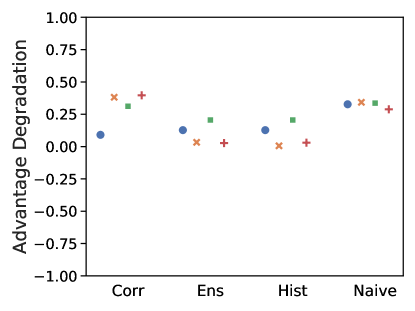
(b)

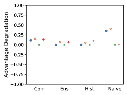
(c)

Figure 2: True SCG: Observe that both causal and non-causal models trained with DP reduce the adversary’s advantage. Causal models provide more advantage degradation on average.

We conduct a toy experiment with synthetic data where the complete (true) causal graph is known apriori. The data is generated based on the SCG defined in Appendix C. The results are presented in Figure 2. Observe that in both the causal and non-causal model, training with DP provides an advantage against the MI adversary, though to varying degrees. We also observe that causal models provide greater resilience on average in comparison to the non-causal model. It is also important to note that the reported value of $\varepsilon$ for the causal model is the same as that of the associational model. Yet, it provides better privacy guarantees. These results confirm our theoretical claim from § 3.1: perfect causal information incorporated with DP provides boosted privacy, even against against real world adversaries. Our results also demonstrate that $\varepsilon$ cannot be used as a sole measure to gauge the privacy of a generative model. The theoretical guarantees of $\varepsilon$-DP do not always translate to resilience against membership attacks in practice.

6.2.2 With Partial Causal Graph

Many real-world datasets do not come with their associated SCGs. Learning these graphs is also a computationally expensive process. To this end, we utilize information from domain experts to partially construct a causal graph. Recall that our theoretical insight implicitly assumes that the information contained by the causal graph is holisitc and accurate. Our evaluation in this subsection verifies if the theory holds when the assumptions are violated. By partial, we mean that nodes for several variables are clubbed together to reduce the overall size of the SCG. Increasing the size of the SCG increases complexity associated with training models; resolving these issues is orthogonal to our work. Note that due to space constraints, we only report results for 2 out of the 3 datasets we evaluate. The trends from Pain1000 are similar to that of Pain5000 and are omitted for brevity. These results can be found in Appendix E.

(a)

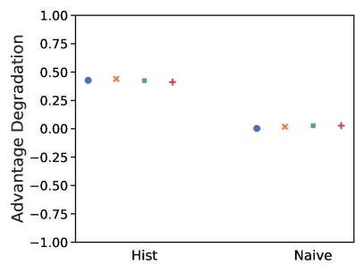
(b)

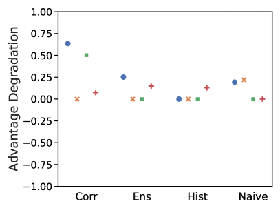
(c)

Figure 3: Effect of DP, No Causality: We plot the advantage degradation when the adversary uses a non-DP trained model and switches to its DP counterpart. Observe that DP enhances the defender’s resilience.

1. Effect of DP.

Figure 3 plots the influence of differential private training on the MI adversary. In particular, we plot how the adversary’s advantage changes when the defender switches from a model trained without DP to one that is trained with DP. A positive value indicates that DP model is more prohibitive to the adversary. We observe that the adversary’s advantage is reduced to varying degrees across both datasets. This suggests that DP training is a reliable defense against adversary’s of this nature (Mukherjee et al., 2019; Bhowmick et al., 2018), despite having a higher range of $\varepsilon$ values (as shown in Table 1). The detailed MI accuracy numbers with precision and recall are in Appendix F.

(a)

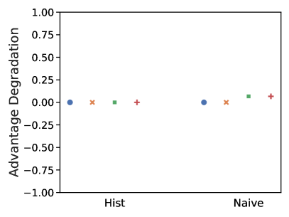
(b)

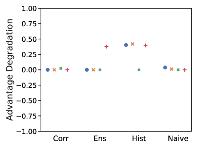
(c)

Figure 4: Partial Causal Information & No DP: We plot the advantage degradation when the adversary uses a non-causal model and switches to its causal counterpart. Observe that even in the absence of DP, causal consistency by itself provides resilience against our MI adversary.

2. Effect of only Causality.

Figure 4 shows the MI adversary’s advantage when the model incorporates causal information in the absence of any DP. Observe that across both datasets, the adversary’s advantage degrades (i.e., has values above zero). While this effect is moderate in the EEDI dataset (Figure 4(b)), this effect is more pronounced in the Pain5000 dataset (Figure 4(c)). This suggests that standalone causal information provides some privacy guarantees. We conjecture that the MI adversary uses the spurious correlation among the attributes to perform the attack. Causal learning algorithms by design eliminate any spurious correlation present in the dataset and hence, a causally consistent VAE is also able to reduce the MI adversary’s advantage.

3. Effect of Causality with DP.

Figure 5 shows the results for models trained using partial causal information with DP and we observe some interesting findings. Similar to the results with complete causal information, we observe that the combination of causality with DP is indeed effective in reducing the MI adversary’s advantage for majority of the feature extractors and classifiers (shown in Figure 5(c) and Figure 5(b) (Hist)). However, as an exception, we see that their conjunction does increase the attacker’s advantage for certain feature extractors when used with specific classifier (such as svc or svc kernel using Naive features in Figure 5(b)). Thus, in this setting, the behaviour is not well explained. We conjecture two reasons for this:

1. The membership inference adversary may exploit spurious correlations between different attributes in a record, and different records. The partial causal information provided does not entirely eliminate these correlations.

2. The information contained in the graph is counteracted by DP training.

(a)

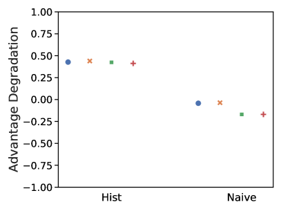
(b)

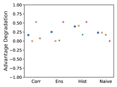
(c)

Figure 5: Partial Causal Information & DP: We plot the advantage degradation when the adversary uses a non-causal model and switches to its causal counterpart. Observe that in the presence of DP & causal consistency, the adversary’s advantage is predominantly reduced. However, there are some cases where the advantage improves by using a causally consistent DP model.

7 Future Work

Through our work, we identify several key questions that are to be analyzed in greater detail.

1. Our approach of incorporating causal information into the generative process has assumed that the SCG is provided. Future work is required to automate the SCG generation process from observed data and directly incorporating it in the VAE training process.

2. In our work, we show that in some scenarios, partial causal information can provide privacy amplification. However, for specific dataset and feature extractor combination, causal information increases attack efficiency used in addition to DP guarantees. A more detailed analysis is required to understand the interplay between partial causal information and DP training.

3. We also wish to understand the influence of incorrect causal information on the efficacy of MI.

8 Related work

Private Data Generation:

The primary issue associated with synthetic data generation in a private manner involves dealing with data scale and dimensionality. Solutions involve using Bayesian networks to add calibrated noise to the latent representations (Zhang et al., 2017; Jälkö et al., 2019), or smarter mechanisms to determine correlations (Zhang et al., 2020b). Utilizing synthetic data generated by generative adversarial networks (GANs) for various problem domains has been extensively studied, but only few solutions provide formal guarantees of privacy (Jordon et al., 2018; Wu et al., 2019; Harder et al., 2020; Torkzadehmahani et al., 2019; Ma et al., 2020b; Tantipongpipat et al., 2019; Xin et al., 2020; Long et al., 2019; Liu et al., 2019). Across the spectrum, very limited techniques are evaluated against adversaries (Mukherjee et al., 2019).

Membership Inference:

Membership Inference (MI) is the process associated with determining whether a particular sample was used in the training of an ML model. This is a more specific form of model inversion (Fredrikson et al., 2014), and was made popular by the work of Shokri et al. (2017). Yeom et al. (2018) draw the connections to MI and overfitting, and argue that differentially private training be a candidate solution. However, most work focuses on the discriminative setting. More recently, several works propose MI attacks against generative models (Stadler et al., 2020; Hayes et al., 2019; Chen et al., 2020; Hilprecht et al., 2019) but offer a limited explanation as to why they are possible.

9 Conclusions

In this work, we propose a mechanism for private data release using VAEs trained with differential privacy. Our theoretical results highlight how causal information encoded into the training procedure can potentially amplify the privacy guarantee provided by differential privacy, without degrading utility. Our results show how knowledge of the true causal graph enables resilience against strong membership inference attacks. However, partial causal knowledge sometimes enhances the adversary. Through this body of work, we wish to better understand why membership inference is possible, and conditions (imposed by causal models) where such attacks fail.

Appendix A Proof of Theorem 1

Notation: A mechanism $H$ takes in as input a dataset $D$ and outputs a parameterized model $f_{\theta}$, where $\theta$ are the parameters of the model. The model (and its parameters) belongs to a hypothesis space $\mathcal{H}$. The dataset comprises of samples, where each sample $\mathbf{x}=(x_{1},\cdots,x_{k})$ comprise of $k$ features. To learn the model, we utilize the empirical risk mechanism (ERM), and a loss function $\mathcal{L}$. The subscript of the loss function denotes what the loss is calculated over. For example $\mathcal{L}_{\mathbf{x}}$ denotes the loss being calculated over sample $\mathbf{x}$. Similarly, $\mathcal{L}_{D}$ denotes the average loss calculated over all samples in the dataset i.e. $\mathcal{L}_{D}=\frac{1}{|D|}\sum_{\mathbf{x}\in D}\mathcal{L}_{\mathbf{x}}$. Additionally, $\mathcal{L}_{\mathbf{x}}(f_{\theta})=l(f_{\theta}(\mathbf{x}),f^{*}(\mathbf{x}))$ where $f^{*}$ is the oracle (responsible for generating ground truth), and $l(.,.)$ can be any loss function (such as the cross entropy loss or reconstruction loss for a generative model).

Data Generating Process (DGP): DGP $<f^{*},\eta>$ is obtained as follows: $f^{*}=\lim_{n\to\infty}\operatorname*{arg\,min}\mathcal{L}_{D}(f_{\theta})$. Essentially $f^{\star}$ can be thought of as the infinite data limit of the ERM learner and can be viewed as the ground truth. In a causal setting, the DGP for all variables/features $\mathbf{x}$ is defined as $f^{*}(\mathbf{x})=(f^{*}_{1}(Pa(x_{1}))+\eta_{i},\cdots,f^{*}_{n}(Pa(x_{n}))+\eta_{n})$ where $\eta_{i}$ are mutually, independently chosen noise values and $Pa(x_{i})$ are the parents of $x_{i}$ in the SCG.

Distinction between Causal and Associational Worlds: For each feature $x_{i}$, we call $Pa(x_{i})$ as the causal features, and $X\setminus\{x_{i},Pa(x_{i})\}$ as the associational features for predicting $x_{i}$. Correspondingly, the model using only $Pa(x_{i})$ for each feature $x_{i}$ is known as the causal model, and the model using all features $X$ (including associational features) is known as the associational model. We denote the causal model learnt by ERM with loss $\mathcal{L}$ as $f_{\theta_{c}}$, and the associational model learnt by ERM using the same loss $\mathcal{L}$ as $f_{\theta_{a}}$. Note that the hypothesis class for the models is different: $f_{\theta_{c}}\in\mathcal{H}_{C}$ and $f_{\theta_{a}}\in\mathcal{H}_{A}$, where $\mathcal{H}_{C}\subseteq\mathcal{H}_{A}$.

Like $f_{\theta_{c}}$, the true DGP function uses only the causal features. Assuming that the true function $f^{*}$ belongs in the hypothesis class $\mathcal{H}_{C}$, we write, $f^{*}=\lim_{|D|\to\infty}\arg\min_{f\in\mathcal{H}_{C}}\mathcal{L}_{D}(f)$.

Adversary. Given a dataset $D$ and a model $f_{\theta}$, the role of an adversary is to create a neighboring dataset $D^{\prime}$ by adding a new point $\mathbf{x}^{\prime}$. We assume that the adversary does so by choosing a point $\mathbf{x}^{\prime}$ where the loss of $f_{\theta}$ is maximized. Thus, the difference of the empirical loss on $D^{\prime}$ compared to $D$ will be high, which we expect to lead to high susceptibility to membership inference attacks.

Definition: Loss-maximizing (LM) Adversary: Given a model $f_{\theta}$, dataset $D$, and a loss function $\mathcal{L}$, an LM adversary chooses a point $\mathbf{x}^{\prime}$ (to be added to $D$ to obtain $D^{\prime}$) as $\arg\max_{\mathbf{x}}\mathcal{L}_{\mathbf{x}}(f_{\theta})$. Note that $\mathcal{L}_{\mathbf{x}}(f_{\theta})=\mathcal{L}_{\mathbf{x}}(f_{\theta}(\mathbf{x}))$

The main steps of our proof are as follows:

1. We show that the maximum loss of a causal model is lower than or equal to maximum loss of the corresponding associational model.

2. Using strong convexity and Lipschitz continuity of the loss function, we show how the difference in loss corresponds to the sensitivity of the learning function.

3. Finally, the privacy budget $\varepsilon$ is a monotonic function of the sensitivity.

We show claim 1 separately for $n\to\infty$ (A.1) and finite $n$ (A.2) below. Then we prove claim 2 in A.3. The claim 3 follows from differential privacy literature  (Dwork et al., 2014).

A.1 Proof of Claim 1 ($n\to\infty$)

As $|D|=n\to\infty$, the proof argument is that the causal model becomes the same as the true DGP $f^{*}$.

P1. Given any variable $x_{t}$, the causal model learns a function based only on its parents, $Pa(x_{t})$. The adversary for causal model chooses points from the DGP $<f^{*},\eta>$ s.t.,

$$\mathbf{x}^{\prime}=\arg\max_{\mathbf{x}}\mathcal{L}_{\mathbf{x}}(f_{\theta_{c}}(\mathbf{x}))\text{ s.t. }\forall i\text{ \ }x_{i}=f_{i}^{*}(Pa(x_{i}))+\eta_{i}$$ (2)

where $f_{\theta_{c}}=\arg\min_{f\in\mathcal{H}_{C}}\mathcal{L}_{D}(f)$. Assuming that $\mathcal{H}_{C}$ is expressive enough such that $f^{*}\in\mathcal{H_{C}}$, as $n=|D|\to\infty$, we can write,

$$\lim_{|D|\to\infty}f_{\theta_{c}}=\lim_{|D|\to\infty}\arg\max_{f\in\mathcal{H}_{C}}\mathcal{L}_{D}(f)=f^{*}$$

Therefore, the causal model is equivalent to the true DGP’s function. For any target $x_{i}$ to be predicted, maximum error on any point is $\eta_{i}$ for the $\ell_{1}$ loss, and a function of $\eta_{i}$ for other losses. Intuitively, the adversary is constrained to choose points at a maximum $\eta_{i}$ distance away from the causal model.

But for associational models, we have,

$$\mathbf{x}^{\prime\prime}=\arg\max_{\mathbf{x}}\mathcal{L}_{\mathbf{x}}(f_{\theta_{a}}(\mathbf{x}))\text{ s.t. }\forall i\text{ \ }x_{i}=f_{i}^{*}(Pa(x_{i}))+\eta_{i}$$ (3)

As $n=|D|\to\infty$, $f_{\theta_{a}}\neq f^{*}$. Thus, the adversary is less constrained and can generate points for a target $x_{i}$ that are generated from a different function than the associational model. For any point, the difference in the associational model’s prediction and the true value is $|f_{\theta_{a}}(\mathbf{x}))-f^{*}(Pa(x_{i}))|+\eta_{i}$, which is equivalent to the loss under $\ell_{1}$. For a general loss function, the loss is a function of $|f_{\theta_{a}}(\mathbf{x})-f^{*}(Pa(x_{i}))|+\eta_{i}$. Therefore, we obtain,

$$\forall i\text{ \ }\eta_{i}\leq|f_{\theta_{a}}(\mathbf{x})-f^{*}(Pa(x_{i}))|+\eta_{i}\Rightarrow\max_{\mathbf{x}}\mathcal{L}_{\mathbf{x}}(f_{\theta_{c}}(\mathbf{x}))\leq\max_{\mathbf{x}}\mathcal{L}_{\mathbf{x}}(f_{\theta_{a}}(\mathbf{x}))$$ (4)

for all losses that are increasing functions of the difference between the predicted and actual value.

A.2 Proof of Claim 1 (Finite $n$)

When $n$ is finite, the proof argument remains the same but we need an additional assumption on the associational model $f_{\theta_{a}}$ learnt from $D$. From learning theory  (Shalev-Shwartz & Ben-David, 2014), we know that the loss of $f_{\theta_{c}}$ will converge to that of $f^{*}$, while loss of $f_{\theta_{a}}$ will converge to loss of $f^{\infty}_{\theta_{a}}\neq f^{*}$. Thus, with high probability, $f_{\theta_{c}}$ will have a lower loss w.r.t. $f^{*}$ than $f_{\theta_{a}}$ and a similar argument follows as for the infinite-data case. However, since this convergence is probabilistic and depends on the size of $n$, it is possible to obtain a $f_{\theta_{c}}$ that has a higher loss w.r.t. $f^{*}$ compared to $f_{\theta_{a}}$.

Therefore, rather than assuming convergence of $f_{\theta_{c}}$ to $f^{*}$, we instead rely on the property that the true DGP function $f^{*}$ does not depend on the associational features $x_{a}$. As a result, even if the loss of the associational model is lower than the causal model on a particular point $\mathbf{x}=x_{c}\cup x_{a}$, we can change the value of $x_{a}$ to obtain a higher loss for the associational model (without changing the loss of the causal model). This requires that the associational model have a non-trivial contribution from the associational (non-causal) features, sufficient to change the loss. We state the following assumption.

Assumption 1: If $f_{\theta_{c}}$ is the causal model and $f_{\theta_{a}}$ is the associational model, then we assume that the associational model has non-trivial contribution from the associational features. Specifically, denote $x_{c}$ as the causal features and $x_{a}$ as the associational features, such that $\mathbf{x}=x_{c}\cup x_{a}$. We define any two new points: $\mathbf{x^{\prime}}=x^{\prime}_{c}\cup x_{a}$ and $\mathbf{x^{\prime\prime}}=x^{\prime\prime}_{c}\cup x^{\prime\prime}_{a}$. Let us first assume a fixed value of $x_{a}$. The LHS (below) denotes the max difference in loss between $f_{\theta_{c}}$ and $f_{\theta_{a}}$ (i.e., change in loss between causal and associational models over the same causal features). The RHS (below) denotes difference in loss of $f_{\theta_{a}}$ between $x_{a}$ and another value $x^{*}_{a}$, keeping $x_{c}$ constant (i.e., effect due to the associational features).

The inequality below can be interpreted as follows: if adversary 1 aims to find the $x^{\prime}_{c}$ such that difference in loss between associational and causal features is highest for a given $x_{a}$, then there can always be another adversary 2 who can obtain a bigger difference in loss by changing the associational features (from the same $x_{a}$ to $x^{\prime\prime}_{a}$).

$$\begin{split}\exists x_{a}\text{\ \ \ }\max_{x^{\prime}_{c}}&\{\mathcal{L}_{\mathbf{x^{\prime}}}(f_{\theta_{c}}(x^{\prime}_{c}\cup x_{a}))-\mathcal{L}_{\mathbf{x^{\prime}}}(f_{\theta_{a}}(x^{\prime}_{c}\cup x_{a}))\}\\ &\leq\min_{x^{\prime\prime}_{c}}\max_{x^{\prime\prime}_{a}}\mathcal{L}_{\mathbf{x}^{\prime\prime}}(f_{\theta_{a}}(x^{\prime\prime}_{c}\cup x^{\prime\prime}_{a}))-\mathcal{L}_{x^{\prime\prime}_{c}\cup x_{a}}(f_{\theta_{a}}(x^{\prime\prime}_{c}\cup x_{a}))\end{split}$$ (5)

Intuition: Imagine that $f_{\theta_{c}}$ is trained initially, and then associational features are introduced to train $f_{\theta_{a}}$. $f_{\theta_{a}}$ can obtain a lower loss than $f_{\theta_{c}}$ by using the associational features $x_{a}$. In doing so, it might even change the model parameters related to $x_{c}$. Assumption 1 says that change in $x_{c}$’s parameters is small compared to the importance of the $x_{a}$’s parameters in $f_{\theta_{a}}$. For example, consider a $f^{*}$, $f_{\theta_{c}}$, $f_{\theta_{a}}$ to predict the value of $x_{t}$ such that $x_{c}=\{x_{1}\}$ and $x_{a}=\{x_{2}\}$, and consider $\ell_{1}$ loss.

$$f^{*}=x_{1}\text{;\ \ \ }f_{\theta_{c}}=2x_{1}\text{;\ \ \ }f_{\theta_{a}}=1.9x_{1}+\phi(x_{2})$$

where $x_{t}=f^{*}(\mathbf{x})+\eta$ and $\eta\in[-0.5,0.5]$. Note that without $\phi(x_{2})$, the loss of the associational model is lower than the loss of causal model on any point. However, if $x_{a}=x_{2}\in\mathbb{R}$, then we can always set $|x_{2}|$ to an extreme value such that $\phi(x_{2})$ overturns the reduction in loss for the associational model, without invoking Assumption 1. When $x_{a}$ is bounded (e.g., $x_{2}\in\{0,1\}$), then Assumption 1 states that the change in loss possible due to changing $\phi(x_{2})$ is higher than the loss difference (which is $0.1$ for $\ell_{1}$ loss). If $\mathcal{H}$ was the class of linear functions and we assume $\ell_{1}$ loss with all features in the same range(e.g., $[0,1]$), then Assumption 1 implies that the coefficient of the associational features in $f_{\theta_{a}}$ is higher than the change in coefficient for the causal features from $f_{\theta_{c}}$ to $f_{\theta_{a}}$.

Proof: Before we discuss the proof, let us establish a few preliminaries.

P2. Let us write $f_{\theta_{a}}(\mathbf{x})=f_{\theta_{a}}(x_{c}\cup x_{a})$ as a combination of terms due to $x_{c}$ and $x_{a}$, where $x_{c}$ and $x_{a}$ are the causal features (parents) and non-causal features respectively i.e. $x_{c}\cup x_{a}=\mathbf{x}$, and $x_{c}\cap x_{a}=\phi$. Let $\mathbf{x}^{\prime}=x^{\prime}_{c}\cup x^{\prime}_{a}$ be the point chosen by the causal adversary.

We will show that the associational adversary can always choose a point $\mathbf{x}^{\prime\prime}=x^{\prime}_{c}\cup x^{\prime\prime}_{a}$ such that loss of the adversary is higher. We write, for any value $x_{a}$,

$$\begin{split}\mathcal{L}(f_{\theta_{a}}(x^{\prime}_{c}\cup x^{\prime\prime}_{a}))&=\mathcal{L}(f_{\theta_{a}}(x^{\prime}_{c}\cup x^{\prime\prime}_{a}))-\mathcal{L}(f_{\theta_{a}}(x^{\prime}_{c}\cup x_{a}))+\mathcal{L}(f_{\theta_{a}}(x^{\prime}_{c}\cup x_{a}))\\ &=(\mathcal{L}(f_{\theta_{a}}(x^{\prime}_{c}\cup x^{\prime\prime}_{a}))-\mathcal{L}(f_{\theta_{a}}(x^{\prime}_{c}\cup x_{a})))+(\mathcal{L}(f_{\theta_{a}}(x^{\prime}_{c}\cup x_{a}))\\ &-\mathcal{L}(f_{\theta_{c}}(x^{\prime}_{c}\cup x_{a})))+\mathcal{L}(f_{\theta_{c}}(x^{\prime}_{c}\cup x_{a}))\end{split}$$ (7)

Rearranging terms, and since $\mathcal{L}(f_{\theta_{c}}(x^{\prime}_{c}\cup x^{\prime}_{a}))=\mathcal{L}(f_{\theta_{c}}(x^{\prime}_{c}\cup x_{a}))$ for any value of $x_{a}$ (causal model does not depend on associational features),

$$\begin{split}\mathcal{L}(f_{\theta_{a}}(x^{\prime}_{c}\cup x^{\prime\prime}_{a}))-\mathcal{L}(f_{\theta_{c}}(x^{\prime}_{c}\cup x^{\prime}_{a}))&=\underbrace{(\mathcal{L}(f_{\theta_{a}}(x^{\prime}_{c}\cup x^{\prime\prime}_{a}))-\mathcal{L}(f_{\theta_{a}}(x^{\prime}_{c}\cup x_{a})))}_{\text{Term 1}}\\ &-\underbrace{(\mathcal{L}(f_{\theta_{c}}(x^{\prime}_{c}\cup x_{a}))-\mathcal{L}(f_{\theta_{a}}(x^{\prime}_{c}\cup x_{a}))}_{\text{Term 2}})\end{split}$$ (8)

Now the first term is $\geq 0$ since the adversary can select $x_{a}^{\prime\prime}$ such that loss increases (or stays constant) for $f_{\theta_{a}}$. Since the true function $f^{*}$ does not depend on $x_{a}$, changing $x_{a}$ does not change the true function’s value but will change the value of the associational model (and adversary can choose it such that loss on the new point is higher). The second term can either be positive or negative. If it is negative, then we are done. Then the LHS $>0$.

If the second term is positive, then we need to show that the first term is higher in magnitude than the second term. From assumption 1, let it be satisfied for some $x^{\circ}_{a}$. We know that $\mathcal{L}(f_{\theta_{c}}(x^{\prime}_{c}\cup x^{\prime}_{a}))=\mathcal{L}(f_{\theta_{c}}(x^{\prime}_{c}\cup x^{\circ}_{a}))$ since the causal model ignores the associational features.

$$\begin{split}\mathcal{L}(f_{\theta_{c}}(x^{\prime}_{c}\cup x^{\circ}_{a}))-\mathcal{L}(f_{\theta_{a}}(x^{\prime}_{c}\cup x^{\circ}_{a}))\leq\max_{x_{c}}(\mathcal{L}(f_{\theta_{c}}(x_{c}\cup x^{\circ}_{a}))-\mathcal{L}(f_{\theta_{a}}(x_{c}\cup x^{\circ}_{a})))\\ \leq\min_{x_{c}}\max_{x^{*}_{a}}(\mathcal{L}(f_{\theta_{a}}(x_{c}\cup x^{*}_{a})-\mathcal{L}(f_{\theta_{a}}(x_{c}\cup x^{\circ}_{a}))\leq\max_{x^{*}_{a}}(\mathcal{L}(f_{\theta_{a}}(x^{\prime}_{c}\cup x^{*}_{a})-\mathcal{L}(f_{\theta_{a}}(x^{\prime}_{c}\cup x^{\circ}_{a}))\end{split}$$ (9)

Now suppose adversary chooses a point such that $x^{\prime\prime}_{a}=x_{a}^{max}$ where $x_{a}^{max}$ is the arg max of the RHS above. Then Equation 7 can be rewritten as,

$$\begin{split}\mathcal{L}(f_{\theta_{a}}(x^{\prime}_{c}\cup x^{max}_{a}))-\mathcal{L}(f_{\theta_{c}}(x^{\prime}_{c}\cup x^{\prime}_{a}))&=(\mathcal{L}(f_{\theta_{a}}(x^{\prime}_{c}\cup x^{max}_{a}))-\mathcal{L}(f_{\theta_{a}}(x^{\prime}_{c}\cup x^{\circ}_{a})))\\ &-(\mathcal{L}(f_{\theta_{c}}(x^{\prime}_{c}\cup x^{\circ}_{a}))-\mathcal{L}(f_{\theta_{a}}(x^{\prime}_{c}\cup x^{\circ}_{a})))\\ &>0\end{split}$$ (10)

where the last inequality is due to equation 8.

Thus, adversary can always select a different value of $\mathbf{x}=x^{\prime}_{c}\cup x_{a}^{max}$ such that loss is higher than the max loss in a causal model.

$$\mathcal{L}(f_{\theta_{c}}(x^{\prime}_{c}\cup x^{\prime}_{a}))=\max_{\mathbf{x}}\mathcal{L}_{\mathbf{x}}(f_{\theta_{c}})\leq\mathcal{L}(f_{\theta_{a}}(x^{\prime}_{c}\cup x^{max}_{a}))\leq\max_{\mathbf{x}}\mathcal{L}_{\mathbf{x}}(f_{\theta_{a}})$$

A.3 Proof of Claim 2

Proof: The proof uses strongly convex and Lipschitz properties of the loss function. Before we discuss the proof, let us introduce some preliminaries.

P1. Assume the existence of a dataset $D$ of size $n$. There are two generative models learnt, $f_{\theta{}_{a}}$ and $f_{\theta{}_{c}}$ using this dataset. Similarly, assume there is a neighboring dataset $D^{\prime}$ which is obtained by adding one point $\mathbf{x}^{\prime}$. Then the corresponding ERM models learnt using $D^{\prime}$ are $f_{\theta{}_{a}^{\prime}}$ and $f_{\theta{}_{c}^{\prime}}$.

We now detail the steps of the proof.

S1. Assume $\mathcal{L}$ is strongly convex. Then by the optimality of ERM predictor on $D$ and the definition of strong convexity,

$$\begin{split}&\mathcal{L}_{D}(f_{\theta})\leq\mathcal{L}_{D}(\alpha f_{\theta}+(1-\alpha)f_{\theta^{\prime}})\\ &\leq\alpha\mathcal{L}_{D}(f_{\theta})+(1-\alpha)\mathcal{L}_{D}(f_{\theta^{\prime}})-\frac{\lambda}{2}\alpha(1-\alpha)||\theta-\theta^{\prime}||^{2}\end{split}$$ (12)

Rearranging terms, and as $\alpha\to 1$,

$$\begin{split}(1-\alpha)\mathcal{L}_{D}(f_{\theta})\leq(1-\alpha)\mathcal{L}_{D}(f_{\theta^{\prime}})-\frac{\lambda}{2}\alpha(1-\alpha)||\theta-\theta^{\prime}||^{2}\\ \Rightarrow||\theta-\theta^{\prime}||^{2}\leq\frac{2}{\lambda}(\mathcal{L}_{D}(f_{\theta^{\prime}})-\mathcal{L}_{D}(f_{\theta}))\end{split}$$ (13)

S3. Further, we can write $(\mathcal{L}_{D}(f_{\theta^{\prime}})-\mathcal{L}_{D}(f_{\theta}))$ in terms of loss on $\mathbf{x}^{\prime}$.

$$\begin{split}\mathcal{L}_{D^{\prime}}(f_{\theta})&=\frac{n}{n+1}\mathcal{L}_{D}(f_{\theta})+\frac{1}{n+1}\mathcal{L}_{\mathbf{x}^{\prime}}(f_{\theta})\text{ (since $D^{\prime}=D\cup\mathbf{x^{\prime}}$)}\\ &\leq\frac{n}{n+1}\mathcal{L}_{D}(f_{\theta^{\prime}})+\frac{1}{n+1}\mathcal{L}_{\mathbf{x}^{\prime}}(f_{\theta})\text{ (from Equation~{}\ref{eq:ref}) }\\ &\leq\frac{n}{n+1}\frac{n+1}{n}\mathcal{L}_{D^{\prime}}(f_{\theta^{\prime}})-\frac{n}{n+1}\frac{1}{n}\mathcal{L}_{\mathbf{x}^{\prime}}(f_{\theta^{\prime}})+\frac{1}{n+1}\mathcal{L}_{\mathbf{x}^{\prime}}(f_{\theta})\text{ (since $D=D^{\prime}-\{\mathbf{x^{\prime}}\}$)}\\ \Rightarrow\mathcal{L}_{D^{\prime}}(f_{\theta})-\mathcal{L}_{D^{\prime}}(f_{\theta^{\prime}})&\leq\frac{1}{n+1}(\mathcal{L}_{\mathbf{x}^{\prime}}(f_{\theta})-\mathcal{L}_{\mathbf{x}^{\prime}}(f_{\theta^{\prime}}))\end{split}$$ (14)

S4. Combining the above two equations, we obtain,

$$||\theta-\theta^{\prime}||^{2}\leq\frac{2}{\lambda}(\mathcal{L}_{D}(f_{\theta^{\prime}})-\mathcal{L}_{D}(f_{\theta}))\leq\frac{2}{\lambda(n+1)}(\mathcal{L}_{\mathbf{x}^{\prime}}(f_{\theta})-\mathcal{L}_{\mathbf{x}^{\prime}}(f_{\theta^{\prime}}))$$ (15)

S5. From Claim 1 above, we know that

$$\begin{split}\max_{\mathbf{x}}\mathcal{L}_{\mathbf{x}}(f_{\theta_{c}})&\leq\max_{\mathbf{x}}\mathcal{L}_{\mathbf{x}}(f_{\theta_{a}})\\ \Rightarrow\mathcal{L}_{\mathbf{x^{\prime}}}(f_{\theta_{c}})&\leq\mathcal{L}_{\mathbf{x^{\prime\prime}}}(f_{\theta_{a}})\end{split}$$ (16)

where $\mathbf{x}^{\prime}=\arg\max_{\mathbf{x}}\mathcal{L}_{\mathbf{x}}(f_{\theta_{c}})$ and $\mathbf{x}^{\prime\prime}$ is chosen such that $\mathbf{x^{\prime}}$ and $\mathbf{x^{\prime\prime}}$ differ only in the associational features. Thus, $\mathcal{L}_{\mathbf{x}^{\prime}}(f_{\theta_{c}^{\prime}})=\mathcal{L}_{\mathbf{x}^{\prime\prime}}(f_{\theta_{c}^{\prime}})$. Also because $\mathcal{H}_{C}\subseteq\mathcal{H}_{A}$, the training loss of the ERM model for any $D^{\prime\prime}$ defined using $D$ and $\mathbf{x}^{\prime\prime}$ is higher for a causal model i.e.,

$$\mathcal{L}_{\mathbf{x}^{\prime}}(f_{\theta_{c}^{\prime}})=\mathcal{L}_{\mathbf{x}^{\prime\prime}}(f_{\theta_{c}^{\prime}})\geq\mathcal{L}_{\mathbf{x}^{\prime\prime}}(f_{\theta_{a}^{\prime}})$$ (17)

Therefore, we obtain,

$$\mathcal{L}_{\mathbf{x}^{\prime}}(f_{\theta_{c}})-\mathcal{L}_{\mathbf{x}^{\prime}}(f_{\theta_{c}^{\prime}})=\max_{\mathbf{x}}\mathcal{L}_{\mathbf{x}}(f_{\theta_{c}})-\mathcal{L}_{\mathbf{x}^{\prime}}(f_{\theta_{c}^{\prime}})\leq\mathcal{L}_{\mathbf{x}^{\prime\prime}}(f_{\theta_{a}})-\mathcal{L}_{\mathbf{x}^{\prime\prime}}(f_{\theta_{a}^{\prime}})$$ (18)

So we have now shown that the max loss difference on a point $\mathbf{x}^{\prime}$ for causal ERM models trained on neighboring datasets is lower than the corresponding loss difference over $\mathbf{x}^{\prime\prime}$ for the associational models.

S6. Now we use the Lipschitz property, to claim,

$$\mathcal{L}_{\mathbf{x}^{\prime\prime}}(f_{\theta_{a}})-\mathcal{L}_{\mathbf{x}^{\prime\prime}}(f_{\theta_{a}^{\prime}})\leq\rho||\theta_{a}-\theta_{a}^{\prime}||$$ (19)

S7. Combining Equations 15 (substituting $f_{\theta_{c}}$) and 19, and taking max on the RHS, we get,

$$\begin{split}\max_{D,D^{\prime}}||\theta_{c}-\theta_{c}^{\prime}||^{2}\leq\frac{2}{\lambda(n+1)}\max_{D,D^{\prime}}\mathcal{L}_{\mathbf{x}^{\prime}}(f_{\theta_{c}})-\mathcal{L}_{\mathbf{x}^{\prime}}(f_{\theta_{c}^{\prime}})\\ \leq\frac{2}{\lambda(n+1)}\max_{D,D^{\prime}}\mathcal{L}_{\mathbf{x}^{\prime}}(f_{\theta_{a}})-\mathcal{L}_{\mathbf{x}^{\prime}}(f_{\theta_{a}^{\prime}})\\ \leq\frac{2\rho}{\lambda(n+1)}\max_{D,D^{\prime}}||\theta_{a}-\theta_{a}^{\prime}||\end{split}$$ (20)

$$\Rightarrow\max_{D,D^{\prime}}||\theta_{c}-\theta_{c}^{\prime}||^{2}\leq\frac{2\rho}{\lambda(n+1)}\max_{D,D^{\prime}}||\theta_{a}-\theta_{a}^{\prime}||$$ (21)

For $n+1>\frac{2\rho}{\lambda}$,

$$\max_{D,D^{\prime}}||\theta_{c}-\theta_{c}^{\prime}||^{2}\leq\max_{D,D^{\prime}}||\theta_{a}-\theta_{a}^{\prime}||$$ (22)

Now if $\max_{D,D^{\prime}}||\theta_{c}-\theta_{c}^{\prime}||\geq 1$, then the result follows by taking the square root over LHS. If not, we need a sufficiently large $n$ such that $n+1>\frac{2\rho}{\lambda\max_{D,D^{\prime}}||\theta_{c}-\theta_{c}^{\prime}||}$, then we obtain,

$$\max_{D,D^{\prime}}||\theta_{c}-\theta_{c}^{\prime}||\leq\max_{D,D^{\prime}}||\theta_{a}-\theta_{a}^{\prime}||$$ (23)

Remark on Theorem 1. Theorem 1 depends on two key assumptions: 1) Assumption 1 that constrains associational model to have non-trivial contribution from associational (non-causal) features; and 2) a sufficiently large $n$ as shown above. When any of these assumptions is violated (e.g., a small-$n$ training dataset or an associational model that is negligibly dependent on the associational features), then it is possible that the causal ERM model has higher privacy budget than the associational ERM model.

Appendix B Training Details

B.1 Models

B.1.1 Pain

Encoder:

$$q_{\phi}(z,x_{1}|x_{2})=q_{\phi_{1}}(z|x_{1},x_{2})\cdot q_{\phi_{2}}(x_{1}|x_{2})$$

Decoder:

$$p_{\theta}(x_{2},x_{1},z)=p_{\theta_{1}}(x_{2}|x_{1})\cdot p_{\theta_{2}}(x_{2}|z)\cdot p_{\theta_{3}}(x_{1}|z)$$

B.1.2 EEDI

Encoder:

$$q_{\phi}(z,x_{1}|x_{2})=q_{\phi_{1}}(z|x_{2})$$

Decoder:

$$p_{\theta}(x_{2},x_{1},z)=p(z)\cdot p(x_{1})\cdot p_{\theta_{1}}(x_{2}|z)\cdot p_{\theta_{2}}(x_{2}|x_{1})$$

Note: All encoders and decoders used as part of our experiments comprised of simple feed-forward architectures. In particular, these architectures have 3 layers. All embeddings generated are of size 10. We set the learning rate to be $0.001$.

B.2 Training Parameters

Causality	Dataset	Batch Size	Epochs
$\times$	EEDI	200	1000
$\checkmark$	EEDI	200	1000
$\times$	Pain1000	100	100
$\checkmark$	Pain1000	100	100
$\times$	Pain5000	100	100
$\checkmark$	Pain5000	100	100
$\times$	Synthetic	100	50
$\checkmark$	Synthetic	100	50

Table 3: Training parameters for our experimental evaluation.

Appendix C Structured Causal Graphs

SCG-1: SCG for the Pain dataset. $X_{1}$ denotes the causes of a medical condition, and $X_{2}$ denotes the various conditions.

SCG-2: SCG used by the EEDI. $X_{2}$ denotes the answers to questions and $X_{1}$ is the student meta data such as the year group and school.

Appendix D Utility Evaluation

D.1 Accuracy on Original Data

The results are detailed in Table 4.

Dataset	Non Causal					Causal
	kernel	svc	logistic	rf	knn	kernel	svc	logistic	rf	knn
EEDI	86.93	91.24	88.53	93.8	88.22	87.38	91.46	88.95	93.44	87.92
Pain1000	92.75	94.42	91.56	94.19	88.78	92.69	94.03	91.81	94.28	89.5
Pain5000	95.37	96.53	97.47	93.03	92.14	95.48	96.5	97.39	92.74	92.19

Table 4: Baseline Accuracy calculated on the original (and not synthetic) data. Results presented in Table 2 are based on these values.

D.2 Privacy vs. Utility

In Figure 6, we plot the utility (measured by the average accuracy across the 5 downstream prediction tasks) for both causal and associational models, for varied values of $\varepsilon$ (obtained by reducing the batch size during training). Observe that for a fixed privacy budget, the causal models always have better utility than their associational counterparts.

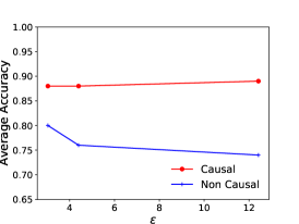
(a)

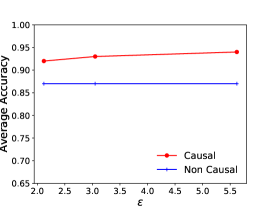
(b)

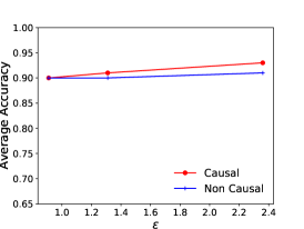
(c)

Figure 6: Utility vs. Privacy: Observe that causal models always outperform their associational counterparts, for the same reported value of $\varepsilon$.

D.3 Pairplots

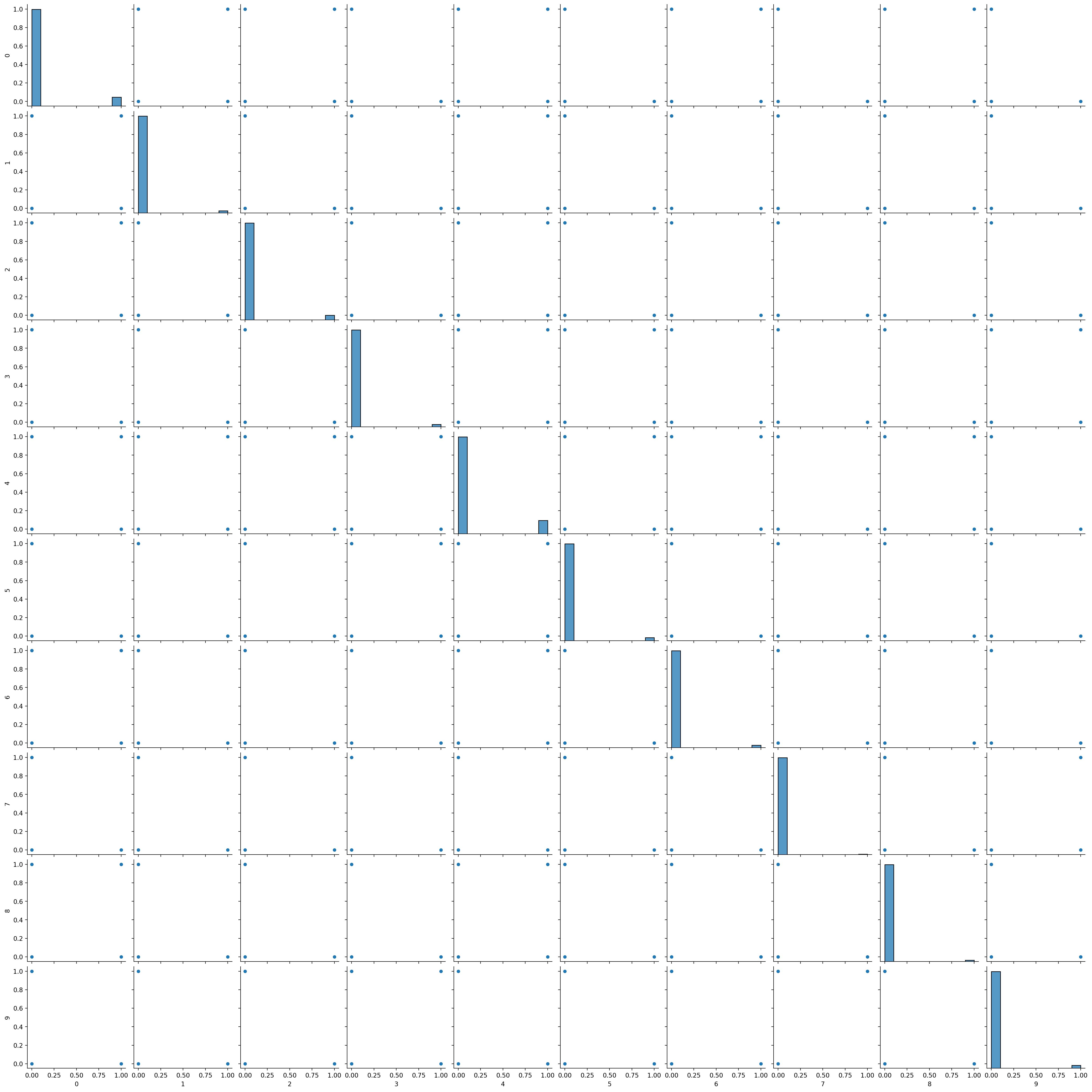
(a)

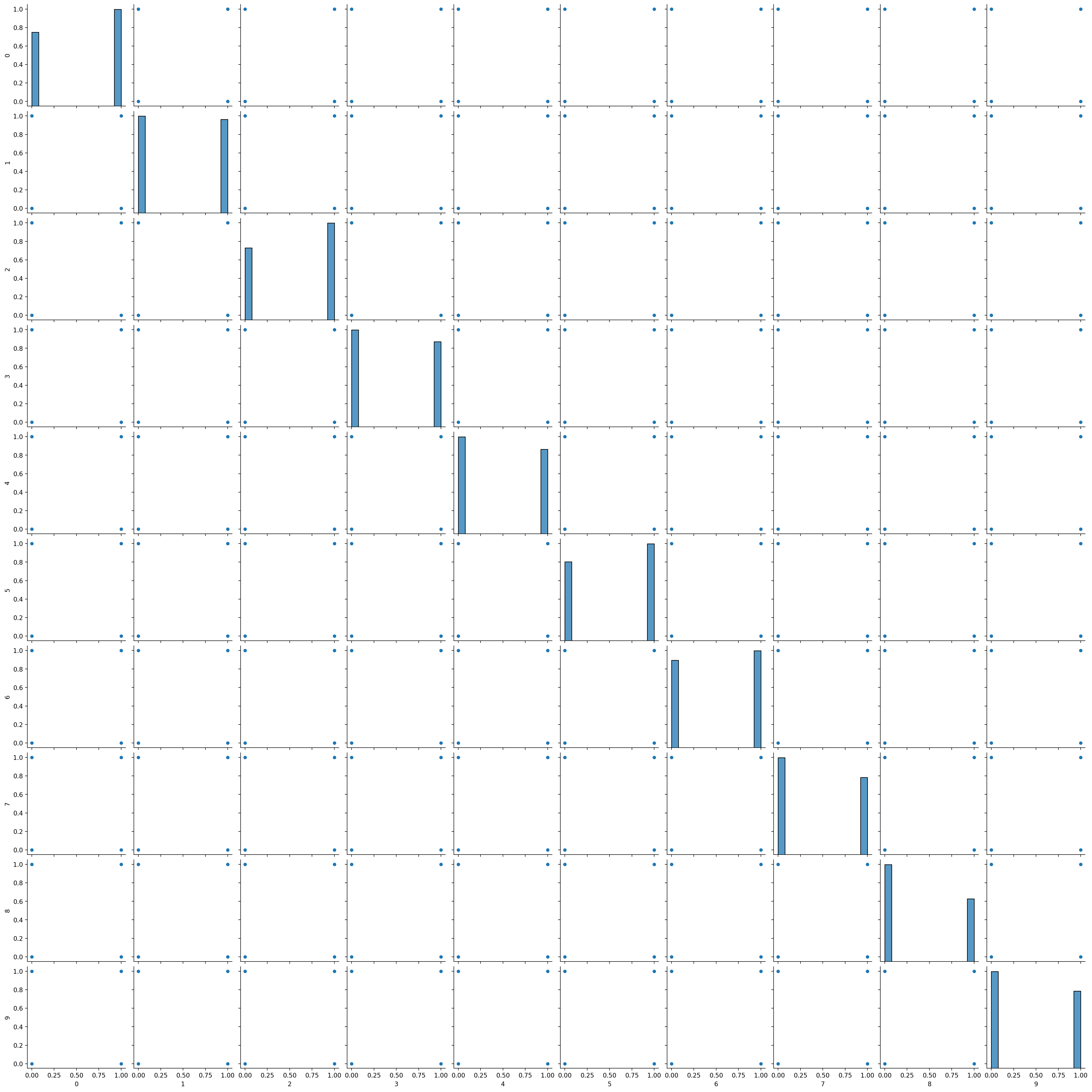
(b)

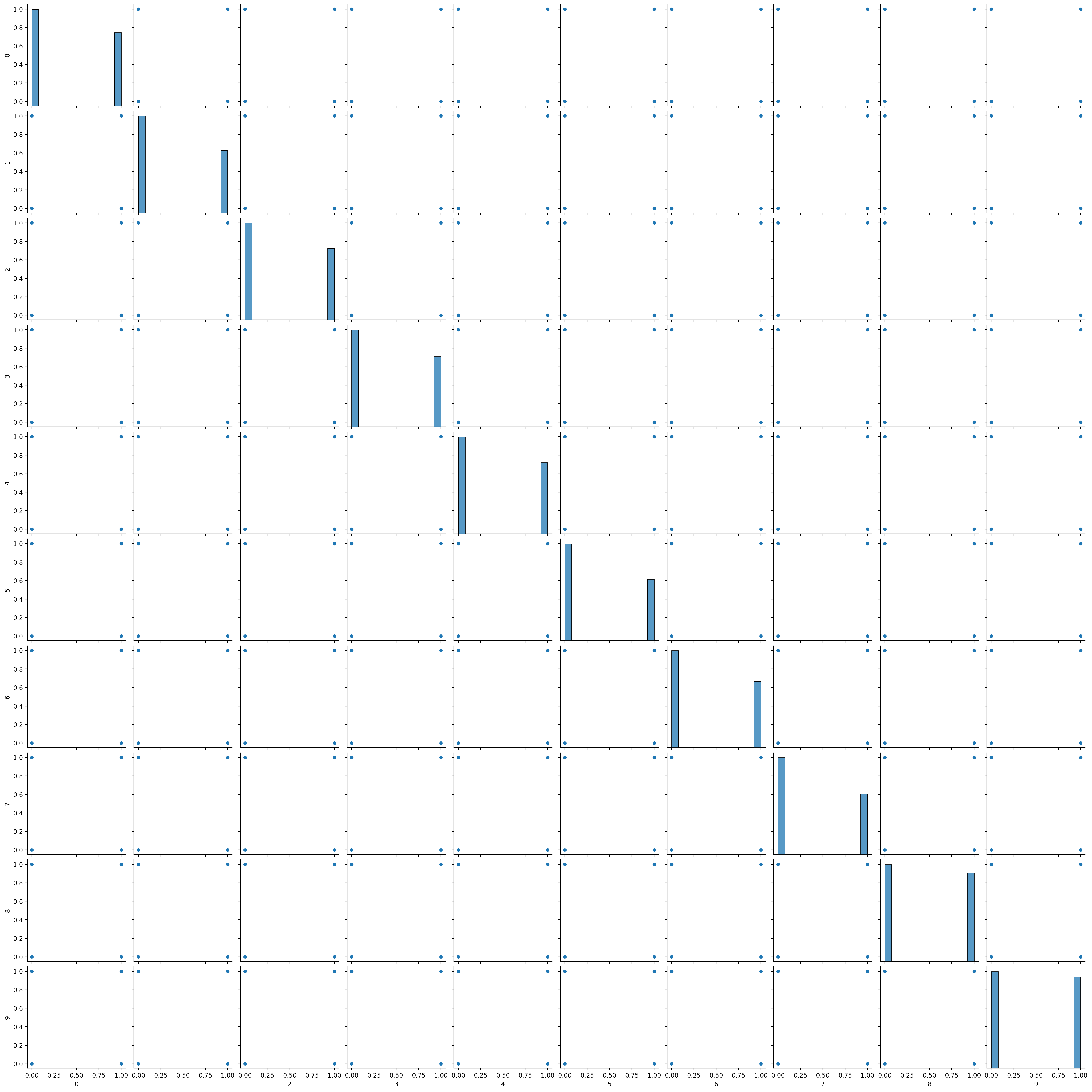
(c)

Figure 7: Pain5000 Dataset

Appendix E Results on Pain1000 Dataset

In Figure 8, we plot the advantage obtained by using only differential privacy (or DP), only causality and causality with DP. Values greater than zero implies that there is a reduction in adversary’s advantage. We observe that DP and causality individually helps mitigate the MI adversary. But the combination of DP with causality, shown in Figure 8(d) helps the adversary with certain classifier and feature extractor combination.

(a)

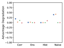
(b)

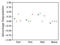
(c)

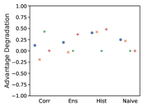
(d)

Figure 8: Impact of DP: Observe that in the causal scenario, DP combined with causal models enables more efficient attacks in some cases.

Takeaway: As discussed in § 6.2.2, partial causal information induces strange artifacts. Additionally, the limited amount of data contained in Pain1000 in comparison to Pain5000 may also contribute to some of these results.

Appendix F MI Results

PA denotes the ability of the classifier to correctly classify train samples. NA denotes the ability of the classifier to correctly classify test samples. The Accuracy is a weighted combination of PA and NA.

EEDI Non Causal:

Refer Table 5.

DP	Extractor	Attack Model	Accuracy	PA	NA
$\checkmark$	Naive	kernel	79.7	76.97	82.42
$\checkmark$	Naive	svc	79.7	76.97	82.42
$\checkmark$	Naive	random forest	98.18	96.97	99.39
$\checkmark$	Naive	knn	99.7	99.39	100.0
$\checkmark$	Histogram	kernel	58.79	100.0	17.58
$\checkmark$	Histogram	svc	57.58	60.61	54.55
$\checkmark$	Histogram	random forest	56.06	30.3	81.82
$\checkmark$	Histogram	knn	57.27	36.36	78.18
$\times$	Naive	kernel	82.42	86.67	78.18
$\times$	Naive	svc	82.42	86.67	78.18
$\times$	Naive	random forest	100.0	100.0	100.0
$\times$	Naive	knn	100.0	100.0	100.0
$\times$	Histogram	kernel	100.0	100.0	100.0
$\times$	Histogram	svc	100.0	100.0	100.0
$\times$	Histogram	random forest	100.0	100.0	100.0
$\times$	Histogram	knn	100.0	100.0	100.0

Table 5: MI Attack accuracy results for EEDI dataset when trained without causal information.

EEDI Causal:

Refer Table 6

DP	Extractor	Attack Model	Accuracy	PA	NA
$\checkmark$	Naive	kernel	62.73	69.09	56.36
$\checkmark$	Naive	svc	62.73	69.09	56.36
$\checkmark$	Naive	random forest	94.55	90.91	98.18
$\checkmark$	Naive	knn	95.45	92.12	98.79
$\checkmark$	Histogram	kernel	100.0	100.0	100.0
$\checkmark$	Histogram	svc	100.0	100.0	100.0
$\checkmark$	Histogram	random forest	100.0	100.0	100.0
$\checkmark$	Histogram	knn	100.0	100.0	100.0
$\times$	Naive	kernel	89.09	78.18	100.0
$\times$	Naive	svc	89.09	78.18	100.0
$\times$	Naive	random forest	100.0	100.0	100.0
$\times$	Naive	knn	100.0	100.0	100.0
$\times$	Histogram	kernel	100.0	100.0	100.0
$\times$	Histogram	svc	100.0	100.0	100.0
$\times$	Histogram	random forest	100.0	100.0	100.0
$\times$	Histogram	knn	100.0	100.0	100.0

Table 6: MI Attack accuracy results for EEDI dataset when trained with causal information

Pain 1000 Causal:

Refer Table 7.

DP	Extractor	Attack Model	Accuracy	PA	NA
$\checkmark$	Naive	kernel	47.33	100.0	0.0
$\checkmark$	Naive	svc	47.33	100.0	0.0
$\checkmark$	Naive	random forest	57.7	60.44	55.24
$\checkmark$	Naive	knn	55.94	60.44	51.9
$\checkmark$	Histogram	kernel	48.3	78.36	21.29
$\checkmark$	Histogram	svc	47.33	100.0	0.0
$\checkmark$	Histogram	random forest	57.82	100.0	19.91
$\checkmark$	Histogram	knn	59.7	81.82	39.82
$\checkmark$	Correlated	kernel	99.7	100.0	99.42
$\checkmark$	Correlated	svc	51.09	83.99	21.52
$\checkmark$	Correlated	random forest	97.39	95.52	99.08
$\checkmark$	Correlated	knn	41.52	42.64	40.51
$\checkmark$	Ensemble	kernel	61.76	20.49	98.85
$\checkmark$	Ensemble	svc	47.33	100.0	0.0
$\checkmark$	Ensemble	random forest	97.94	96.93	98.85
$\checkmark$	Ensemble	knn	81.09	86.3	76.41
$\times$	Naive	kernel	47.33	100.0	0.0
$\times$	Naive	svc	47.33	100.0	0.0
$\times$	Naive	random forest	99.58	99.74	99.42
$\times$	Naive	knn	96.76	96.16	95.4
$\times$	Histogram	kernel	57.82	100.0	19.91
$\times$	Histogram	svc	47.33	100.0	0.0
$\times$	Histogram	random forest	57.82	100.0	19.91
$\times$	Histogram	knn	59.7	81.82	39.82
$\times$	Correlated	kernel	98.24	99.62	97.01
$\times$	Correlated	svc	62.12	50.58	72.5
$\times$	Correlated	random forest	100.0	100.0	100.0
$\times$	Correlated	knn	60.61	60.95	60.3
$\times$	Ensemble	kernel	61.7	72.23	51.78
$\times$	Ensemble	svc	47.33	100.0	0.0
$\times$	Ensemble	random forest	100.0	100.0	100.0
$\times$	Ensemble	knn	82.12	83.99	80.44

Table 7: MI Attack accuracy results for Pain1000 dataset when trained with causal information

Pain 1000 Non Causal:

Refer Table 8.

DP	Extractor	Attack Model	Accuracy	PA	NA
$\checkmark$	Naive	kernel	47.33	100.0	0.0
$\checkmark$	Naive	svc	47.33	100.0	0.0
$\checkmark$	Naive	random forest	79.82	82.33	77.56
$\checkmark$	Naive	knn	80.85	82.71	79.17
$\checkmark$	Histogram	kernel	96.36	96.41	96.32
$\checkmark$	Histogram	svc	47.33	100.0	0.0
$\checkmark$	Histogram	random forest	100.0	100.0	100.0
$\checkmark$	Histogram	knn	100.0	100.0	100.0
$\checkmark$	Correlated	kernel	100.0	100.0	100.0
$\checkmark$	Correlated	svc	94.12	92.83	95.28
$\checkmark$	Correlated	random forest	78.0	79.0	77.1
$\checkmark$	Correlated	knn	53.82	74.9	34.87
$\checkmark$	Ensemble	kernel	98.55	98.46	98.62
$\checkmark$	Ensemble	svc	47.33	100.0	0.0
$\checkmark$	Ensemble	random forest	94.85	93.98	95.63
$\checkmark$	Ensemble	knn	100.0	100.0	100.0
$\times$	Naive	kernel	47.33	100.0	0.0
$\times$	Naive	svc	47.33	100.0	0.0
$\times$	Naive	random forest	99.7	100.0	99.42
$\times$	Naive	knn	85.76	88.6	83.2
$\times$	Histogram	kernel	86.79	90.14	83.77
$\times$	Histogram	svc	47.33	100.0	0.0
$\times$	Histogram	random forest	100.0	100.0	100.0
$\times$	Histogram	knn	94.91	94.88	94.94
$\times$	Correlated	kernel	100.0	100.0	100.0
$\times$	Correlated	svc	100.0	100.0	100.0
$\times$	Correlated	random forest	100.0	100.0	100.0
$\times$	Correlated	knn	73.88	72.73	74.91
$\times$	Ensemble	kernel	98.3	99.49	97.24
$\times$	Ensemble	svc	47.33	100.0	0.0
$\times$	Ensemble	random forest	100.0	100.0	100.0
$\times$	Ensemble	knn	88.79	90.27	87.46

Table 8: MI Attack accuracy results for Pain1000 dataset when trained without causal information

Pain 5000 Causal:

Refer Table 9.

DP	Extractor	Attack Model	Accuracy	PA	NA
$\checkmark$	Naive	kernel	47.33	100.0	0.0
$\checkmark$	Naive	svc	47.33	100.0	0.0
$\checkmark$	Naive	random forest	76.85	78.36	75.49
$\checkmark$	Naive	knn	76.79	78.36	75.37
$\checkmark$	Histogram	kernel	47.33	100.0	0.0
$\checkmark$	Histogram	svc	47.33	100.0	0.0
$\checkmark$	Histogram	random forest	57.82	100.0	19.91
$\checkmark$	Histogram	knn	58.7	81.82	39.82
$\checkmark$	Correlated	kernel	92.61	94.88	90.56
$\checkmark$	Correlated	svc	47.33	100.0	0.0
$\checkmark$	Correlated	random forest	100.0	100.0	100.0
$\checkmark$	Correlated	knn	36.48	45.07	28.77
$\checkmark$	Ensemble	kernel	47.33	100.0	0.0
$\checkmark$	Ensemble	svc	47.33	100.0	0.0
$\checkmark$	Ensemble	random forest	100.0	100.0	100.0
$\checkmark$	Ensemble	knn	74.85	81.56	68.81
$\times$	Naive	kernel	47.33	100.0	0.0
$\times$	Naive	svc	47.33	100.0	0.0
$\times$	Naive	random forest	98.85	97.7	99.88
$\times$	Naive	knn	96.12	93.98	98.04
$\times$	Histogram	kernel	60.24	38.16	80.09
$\times$	Histogram	svc	47.33	100.0	0.0
$\times$	Histogram	random forest	57.82	100.0	19.91
$\times$	Histogram	knn	59.7	81.82	39.82
$\times$	Correlated	kernel	100.0	100.0	100.0
$\times$	Correlated	svc	97.64	100.0	95.51
$\times$	Correlated	random forest	100.0	100.0	100.0
$\times$	Correlated	knn	100.0	100.0	100.0
$\times$	Ensemble	kernel	62.18	46.73	76.06
$\times$	Ensemble	svc	47.33	100.0	0.0
$\times$	Ensemble	random forest	100.0	100.0	100.0
$\times$	Ensemble	knn	100.0	100.0	100.0

Table 9: MI Attack accuracy results for Pain5000 dataset when trained with causal information

Pain 5000 Non Causal:

Refer Table 10.

DP	Extractor	Attack Model	Accuracy	PA	NA
$\checkmark$	Naive	kernel	47.33	100.0	0.0
$\checkmark$	Naive	svc	64.61	60.18	68.58
$\checkmark$	Naive	random forest	99.94	99.87	100.0
$\checkmark$	Naive	knn	100.0	100.0	100.0
$\checkmark$	Histogram	kernel	100.0	100.0	100.0
$\checkmark$	Histogram	svc	65.03	91.55	41.2
$\checkmark$	Histogram	random forest	100.0	100.0	100.0
$\checkmark$	Histogram	knn	100.0	100.0	100.0
$\checkmark$	Correlated	kernel	100.0	100.0	100.0
$\checkmark$	Correlated	svc	100.0	100.0	100.0
$\checkmark$	Correlated	random forest	99.76	99.62	99.88
$\checkmark$	Correlated	knn	53.09	80.41	28.54
$\checkmark$	Ensemble	kernel	100.0	100.0	100.0
$\checkmark$	Ensemble	svc	48.85	100.0	2.88
$\checkmark$	Ensemble	random forest	100.0	100.0	100.0
$\checkmark$	Ensemble	knn	100.0	100.0	100.0
$\times$	Naive	kernel	47.33	100.0	0.0
$\times$	Naive	svc	47.33	100.0	0.0
$\times$	Naive	random forest	100.0	100.0	100.0
$\times$	Naive	knn	99.82	99.62	100.0
$\times$	Histogram	kernel	100.0	100.0	100.0
$\times$	Histogram	svc	47.33	100.0	0.0
$\times$	Histogram	random forest	100.0	100.0	100.0
$\times$	Histogram	knn	100.0	100.0	100.0
$\times$	Correlated	kernel	100.0	100.0	100.0
$\times$	Correlated	svc	100.0	100.0	100.0
$\times$	Correlated	random forest	100.0	100.0	100.0
$\times$	Correlated	knn	100.0	100.0	100.0
$\times$	Ensemble	kernel	100.0	100.0	100.0
$\times$	Ensemble	svc	47.33	100.0	0.0
$\times$	Ensemble	random forest	100.0	100.0	100.0
$\times$	Ensemble	knn	100.0	100.0	100.0

Table 10: MI Attack accuracy results for Pain5000 dataset when trained without causal information

References

- Abadi et al. (2016) Martin Abadi, Andy Chu, Ian Goodfellow, H Brendan McMahan, Ilya Mironov, Kunal Talwar, and Li Zhang. Deep learning with differential privacy. In Proceedings of the 2016 ACM SIGSAC conference on computer and communications security, pp. 308–318, 2016.
- Bhowmick et al. (2018) Abhishek Bhowmick, John Duchi, Julien Freudiger, Gaurav Kapoor, and Ryan Rogers. Protection against reconstruction and its applications in private federated learning. arXiv preprint arXiv:1812.00984, 2018.
- Blei et al. (2017) David M Blei, Alp Kucukelbir, and Jon D McAuliffe. Variational inference: A review for statisticians. Journal of the American statistical Association, 112(518):859–877, 2017.
- Chen et al. (2020) Dingfan Chen, Ning Yu, Yang Zhang, and Mario Fritz. Gan-leaks: A taxonomy of membership inference attacks against generative models. In Proceedings of the 2020 ACM SIGSAC Conference on Computer and Communications Security, pp. 343–362, 2020.
- Cormode et al. (2019) Graham Cormode, Tejas Kulkarni, and Divesh Srivastava. Answering range queries under local differential privacy. Proceedings of the VLDB Endowment, 12(10):1126–1138, 2019.
- Dwork et al. (2006) Cynthia Dwork, Frank McSherry, Kobbi Nissim, and Adam Smith. Calibrating noise to sensitivity in private data analysis. In Theory of cryptography conference, pp. 265–284. Springer, 2006.
- Dwork et al. (2009) Cynthia Dwork, Moni Naor, Omer Reingold, Guy N Rothblum, and Salil Vadhan. On the complexity of differentially private data release: efficient algorithms and hardness results. In Proceedings of the forty-first annual ACM symposium on Theory of computing, pp. 381–390, 2009.
- Dwork et al. (2014) Cynthia Dwork, Aaron Roth, et al. The algorithmic foundations of differential privacy. Foundations and Trends in Theoretical Computer Science, 9(3-4):211–407, 2014.
- Edge et al. (2020) Darren Edge, Weiwei Yang, Harry Cook, Claire Galez-Davis, Hannah Darnton, Kate Lytvynets, and Christopher M. White. Design of a privacy-preserving data platform for collaboration against human trafficking, 2020. https://arxiv.org/abs/2005.05688.
- Fredrikson et al. (2014) Matthew Fredrikson, Eric Lantz, Somesh Jha, Simon Lin, David Page, and Thomas Ristenpart. Privacy in pharmacogenetics: An end-to-end case study of personalized warfarin dosing. In 23rd USENIX Security Symposium (USENIX Security 14), pp. 17–32, 2014.
- Glymour et al. (2019) Clark Glymour, Kun Zhang, and Peter Spirtes. Review of causal discovery methods based on graphical models. Frontiers in genetics, 10:524, 2019.
- Harder et al. (2020) Frederik Harder, Kamil Adamczewski, and Mijung Park. Differentially private mean embeddings with random features (dp-merf) for simple & practical synthetic data generation. arXiv preprint arXiv:2002.11603, 2020.
- Hardt et al. (2010) Moritz Hardt, Katrina Ligett, and Frank McSherry. A simple and practical algorithm for differentially private data release. arXiv preprint arXiv:1012.4763, 2010.
- Hayes et al. (2019) Jamie Hayes, Luca Melis, George Danezis, and Emiliano De Cristofaro. Logan: Membership inference attacks against generative models. Proceedings on Privacy Enhancing Technologies, 2019(1):133–152, 2019.
- Hilprecht et al. (2019) Benjamin Hilprecht, Martin Härterich, and Daniel Bernau. Monte carlo and reconstruction membership inference attacks against generative models. Proceedings on Privacy Enhancing Technologies, 2019(4):232–249, 2019.
- Jälkö et al. (2019) Joonas Jälkö, Eemil Lagerspetz, Jari Haukka, Sasu Tarkoma, Samuel Kaski, and Antti Honkela. Privacy-preserving data sharing via probabilistic modelling. arXiv preprint arXiv:1912.04439, 2019.
- Jordan et al. (1999) Michael I Jordan, Zoubin Ghahramani, Tommi S Jaakkola, and Lawrence K Saul. An introduction to variational methods for graphical models. Machine learning, 37(2):183–233, 1999.
- Jordon et al. (2018) James Jordon, Jinsung Yoon, and Mihaela van der Schaar. Pate-gan: Generating synthetic data with differential privacy guarantees. In International Conference on Learning Representations, 2018.
- Jordon et al. (2020) James Jordon, Daniel Jarrett, Jinsung Yoon, Tavian Barnes, Paul Elbers, Patrick Thoral, Ari Ercole, Cheng Zhang, Danielle Belgrave, and Mihaela van der Schaar. Hide-and-seek privacy challenge. arXiv preprint arXiv:2007.12087, 2020.
- Kingma & Welling (2013) Diederik P Kingma and Max Welling. Auto-encoding variational bayes. arXiv preprint arXiv:1312.6114, 2013.
- Liu et al. (2019) Yi Liu, Jialiang Peng, JQ James, and Yi Wu. Ppgan: Privacy-preserving generative adversarial network. In 2019 IEEE 25th International Conference on Parallel and Distributed Systems (ICPADS), pp. 985–989. IEEE, 2019.
- Long et al. (2019) Yunhui Long, Suxin Lin, Zhuolin Yang, Carl A Gunter, and Bo Li. Scalable differentially private generative student model via pate. arXiv preprint arXiv:1906.09338, 2019.
- Ma et al. (2019) Chao Ma, Sebastian Tschiatschek, Konstantina Palla, Jose Miguel Hernandez-Lobato, Sebastian Nowozin, and Cheng Zhang. Eddi: Efficient dynamic discovery of high-value information with partial vae. In International Conference on Machine Learning, pp. 4234–4243, 2019.
- Ma et al. (2020a) Chao Ma, Sebastian Tschiatschek, José Miguel Hernández-Lobato, Richard Turner, and Cheng Zhang. Vaem: a deep generative model for heterogeneous mixed type data. arXiv preprint arXiv:2006.11941, 2020a.
- Ma et al. (2020b) Chuan Ma, Jun Li, Ming Ding, Bo Liu, Kang Wei, Jian Weng, and H Vincent Poor. Rdp-gan: Ar’enyi-differential privacy based generative adversarial network. arXiv preprint arXiv:2007.02056, 2020b.
- Mukherjee et al. (2019) Sumit Mukherjee, Yixi Xu, Anusua Trivedi, and Juan Lavista Ferres. privgan: Protecting gans from membership inference attacks at low cost, 2019. https://arxiv.org/abs/2001.00071, https://github.com/microsoft/privGAN.
- Peters et al. (2017) Jonas Peters, Dominik Janzing, and Bernhard Schölkopf. Elements of causal inference: foundations and learning algorithms. The MIT Press, 2017.
- Rezende et al. (2014) Danilo Jimenez Rezende, Shakir Mohamed, and Daan Wierstra. Stochastic backpropagation and approximate inference in deep generative models. In International conference on machine learning, pp. 1278–1286. PMLR, 2014.
- Shalev-Shwartz & Ben-David (2014) Shai Shalev-Shwartz and Shai Ben-David. Understanding machine learning: From theory to algorithms. Cambridge university press, 2014.
- Shokri et al. (2017) Reza Shokri, Marco Stronati, Congzheng Song, and Vitaly Shmatikov. Membership inference attacks against machine learning models. In 2017 IEEE Symposium on Security and Privacy (SP), pp. 3–18. IEEE, 2017.
- Spirtes et al. (2000) Peter Spirtes, Clark N Glymour, Richard Scheines, and David Heckerman. Causation, prediction, and search. 2000.
- Stadler et al. (2020) Theresa Stadler, Bristena Oprisanu, and Carmela Troncoso. Synthetic data – a privacy mirage, 2020.
- Tantipongpipat et al. (2019) Uthaipon Tantipongpipat, Chris Waites, Digvijay Boob, Amaresh Ankit Siva, and Rachel Cummings. Differentially private mixed-type data generation for unsupervised learning. arXiv preprint arXiv:1912.03250, 2019.
- Tople et al. (2020) Shruti Tople, Amit Sharma, and Aditya Nori. Alleviating privacy attacks via causal learning. In International Conference on Machine Learning, pp. 9537–9547. PMLR, 2020.
- Torkzadehmahani et al. (2019) Reihaneh Torkzadehmahani, Peter Kairouz, and Benedict Paten. Dp-cgan: Differentially private synthetic data and label generation. In Proceedings of the IEEE Conference on Computer Vision and Pattern Recognition Workshops, pp. 0–0, 2019.
- Tu et al. (2019a) Ruibo Tu, Cheng Zhang, Paul Ackermann, Karthika Mohan, Hedvig Kjellström, and Kun Zhang. Causal discovery in the presence of missing data. In The 22nd International Conference on Artificial Intelligence and Statistics, pp. 1762–1770. PMLR, 2019a.
- Tu et al. (2019b) Ruibo Tu, Kun Zhang, Bo Christer Bertilson, Hedvig Kjellström, and Cheng Zhang. Neuropathic pain diagnosis simulator for causal discovery algorithm evaluation. arXiv preprint arXiv:1906.01732, 2019b.
- Wainwright & Jordan (2008) Martin J Wainwright and Michael Irwin Jordan. Graphical models, exponential families, and variational inference. Now Publishers Inc, 2008.
- Wang et al. (2020) Zichao Wang, Angus Lamb, Evgeny Saveliev, Pashmina Cameron, Yordan Zaykov, José Miguel Hernández-Lobato, Richard E Turner, Richard G Baraniuk, Craig Barton, Simon Peyton Jones, et al. Diagnostic questions: The neurips 2020 education challenge. arXiv preprint arXiv:2007.12061, 2020.
- Woodward (2005) James Woodward. Making things happen: A theory of causal explanation. Oxford university press, 2005.
- Wu et al. (2019) Bingzhe Wu, Shiwan Zhao, Chaochao Chen, Haoyang Xu, Li Wang, Xiaolu Zhang, Guangyu Sun, and Jun Zhou. Generalization in generative adversarial networks: A novel perspective from privacy protection. In Advances in Neural Information Processing Systems, pp. 307–317, 2019.
- Xiao et al. (2010) Yonghui Xiao, Li Xiong, and Chun Yuan. Differentially private data release through multidimensional partitioning. In Workshop on Secure Data Management, pp. 150–168. Springer, 2010.
- Xin et al. (2020) Bangzhou Xin, Wei Yang, Yangyang Geng, Sheng Chen, Shaowei Wang, and Liusheng Huang. Private fl-gan: Differential privacy synthetic data generation based on federated learning. In ICASSP 2020-2020 IEEE International Conference on Acoustics, Speech and Signal Processing (ICASSP), pp. 2927–2931. IEEE, 2020.
- Yeom et al. (2018) Samuel Yeom, Irene Giacomelli, Matt Fredrikson, and Somesh Jha. Privacy risk in machine learning: Analyzing the connection to overfitting. In 2018 IEEE 31st Computer Security Foundations Symposium (CSF), pp. 268–282. IEEE, 2018.
- Zhang et al. (2018) Cheng Zhang, Judith Bütepage, Hedvig Kjellström, and Stephan Mandt. Advances in variational inference. IEEE transactions on pattern analysis and machine intelligence, 41(8):2008–2026, 2018.
- Zhang et al. (2020a) Cheng Zhang, Kun Zhang, and Yingzhen Li. A causal view on robustness of neural networks. arXiv preprint arXiv:2005.01095, 2020a.
- Zhang et al. (2017) Jun Zhang, Graham Cormode, Cecilia M Procopiuc, Divesh Srivastava, and Xiaokui Xiao. PrivBAYES: Private data release via bayesian networks. ACM Transactions on Database Systems (TODS), 42(4):25, 2017. https://dl.acm.org/doi/pdf/10.1145/3134428.
- Zhang et al. (2020b) Zhikun Zhang, Tianhao Wang, Ninghui Li, Jean Honorio, Michael Backes, Shibo He, Jiming Chen, and Yang Zhang. Privsyn: Differentially private data synthesis. arXiv preprint arXiv:2012.15128, 2020b.