Ordered Reference Dependent Choice

Abstract

This paper studies how violations of structural assumptions like expected utility and exponential discounting can be connected to basic rationality violations, even though these assumptions are typically regarded as independent building blocks in decision theory. A reference-dependent generalization of behavioral postulates captures preference shifts in various choice domains. When reference points are fixed, canonical models hold; otherwise, reference-dependent preference parameters (e.g., CARA coefficients, discount factors) give rise to “non-standard” behavior. The framework allows us to study risk, time, and social preferences collectively, where seemingly independent anomalies are interconnected through the lens of reference-dependent choice.

Keywords: Basic rationality, structural postulates, reference dependence, context effects, risk preference, time preference, social preference
JEL: D01, D11

1 Introduction

In various branches of economics, multiple assumptions come together to form the basis of an economic model, and interesting findings often emerge from the unforeseen interplay among these assumptions. The empirical failure of these models, however, need not lie in the substance of each individual assumption but is rooted in their indiscriminate applications.

In individual decision-making, the standard model of choice faces two distinct strands of empirical challenges. First, structural assumptions like the expected utility form and exponential discounting are violated in simple choice experiments, such as the Allais paradox and present bias behavior. Second, and separately, studies show that choices are often affected by reference points, resulting in behavior that violates basic rationality assumptions like the weak axiom of revealed preferences (WARP). With few exceptions, these two classes of departures have been studied separately, and independently for each domain of choice, leading to the development of models that attempt to explain one phenomenon in isolation of the others.

This paper introduces a unified framework that studies how the two types of violations may be in part related to one another, stemming from a common source. The central approach is motivated by a simple observation: Suppose preference parameters (e.g., utility functions capturing risk attitude and discount factors representing degree of patience) are influenced by reference alternatives, then even decision makers who typically adhere to normative postulates (e.g., maximize exponentially discounted expected utility) would every so often violate rationality assumptions and structural assumptions—when reference alternatives change. On the other hand, choices made under the same reference would fully align with both postulates. Thus, while the two types of assumptions are conventionally treated as separate building blocks of a choice model—introduced as independently motivated axioms—their deviations are intrinsically connected by systematic shifts in preferences.

To illustrate, a myriad of documented anomalies, including the Allais paradox, suggests that decision makers exhibit increased risk aversion when presented with safer options (Allais, 1990; Wakker and Deneffe, 1996; Herne, 1999; Bleichrodt and Schmidt, 2002; Andreoni and Sprenger, 2011). While this behavior contradicts the expected utility theory, it aligns with the expected utility framework when coupled with context-dependent utility functions that vary in concavity. This observation motivates the model in the risk domain.

$$c\left(A\right)=\underset{p\in A}{\text{$\arg\max$}}\,\,\sum_{x}p\left(x\right)u_{r}\left(x\right)$$ (1.1)

Standard expected utility applies when the safest alternative, which acts as the reference $r$, is fixed; but when it changes, a safer reference leads to a more concave utility function $u_{r}$, reflecting a systematic increase in risk aversion.

This observation is not exclusive to expected utility. In time preferences, present bias individuals who are less patient in short-term decisions violate exponential discounting (Laibson, 1997; Frederick, Loewenstein, and O’donoghue, 2002; Benhabib, Bisin, and Schotter, 2010; Chakraborty, 2021). However, their behavior could be consistent with the exponential discounting form when paired with context-dependent discount factors that capture changing time preferences.

$$c\left(A\right)=\underset{\left(x,t\right)\in A}{\text{$\arg\max$}}\,\,\delta_{r}^{t}u\left(x\right)$$ (1.2)

When a problem offers sooner payments, it alters the reference point $r$, prompting the decision maker to use a lower discount factor $\delta_{r}$ that reflects increased impatience. Again, changes in preferences are systematic along a certain order, and behavior is otherwise standard.

For social preferences, it is well-documented in economics and psychology that the very same individuals display different degree of altruism in different choice settings, for example when a balanced split of reward is available than when it is not (Ainslie, 1992; Rabin, 1993; Nelson, 2002; Fehr and Schmidt, 2006; Sutter, 2007). These context-dependent preferences could be consistent with

$$c\left(A\right)=\underset{\left(x,y\right)\in A}{\text{$\arg\max$}}\,\,x+v_{r}\left(y\right)$$ (1.3)

where increased altruism is captured by a utility from sharing, $v_{r}\left(\cdot\right)$, that systematically increases when more-equitable splits become the reference.

This paper aims to examine these behaviors as one collective, addressing three key questions: (1) Under what conditions do non-standard behaviors across various choice domains permit such representations? (2) What do they have in common? and (3) How does their systematic departure from canonical models inform the relationship between rationality assumptions and structural assumptions?

It turns out that, although these behavioral anomalies are typically investigated in largely separate and domain-specific studies, the behavioral content of the proposed models is underpinned by a “meta” axiomatic foundation referred to as Reference Dependence (RD). RD is the key innovation of this paper, introducing a reference-dependent approach that can generalize a large class of behavioral postulates or axioms, be it “rational” or “structural”. When applied to the risk, time, and social domains, it yields three complete characterizations that resonate with one another.

To illustrate the idea, 2 applies RD only to rationality assumption by requiring that in every (finite) choice set, at least one alternative would preserve WARP among choice behavior from its subsets. Intuitively, if the failure of rationality is caused by reference dependence, then rationality should continue to hold at least for choice sets that share the same reference. It turns out that this postulate characterizes a two-step choice process: A reference order is maximized to identify the reference alternative $r\left(A\right)$ of a choice problem $A$. The reference alternative then determines a utility function that the decision maker maximizes. Intuitively, the context of a choice problem is captured by the alternative that ranks highest in the reference order and the underlying context-dependent preference is subsequently determined.

$$c\left(A\right)=\underset{z\in A}{\text{$\arg\max$}}\,\,U_{r\left(A\right)}\left(z\right)$$ (1.4)

It has not gone unnoticed that Equations 1.1, 1.2, and 1.3 are special cases of (LABEL:general), sharing two essentially components: (i) a reference order and (ii) reference-dependent preference parameters. It is also apparent that basic rationality—the assumption that one persistent utility function is being maximized—can fail, which makes the proposed explanations not particularly appealing, at least until the recent accumulation of theoretical interest and empirical evidence against basic rationality itself.

It turns out that, barring technical challenges, the axiomatic characterization of each of these behaviors requires little more than adapting RD to their domain-specific normative postulates. For risk preference, Risk-RD preserves both WARP (rationality axiom) and von Neumann-Morgenstern’s Independence (structural axiom) when the safest alternative is maintained. For time preference, Time-RD preserves normative postulates WARP (rationality axiom) and Stationarity (structural axiom) when the earliest available payment is fixed. For social preference, Social-RD calls for consistency with WARP (rationality axiom) and Quasi-linearity (structural axiom) when the most-balanced options coincide. The underlying intuition is universal: Upholding the reference point ensures the validity of all normative postulates, so that violations of structural assumptions—whatever they are and whatever the domain—are linked to reference dependent preferences manifested in basic rationality violations. A second axiom, which does not involve reference points, captures systematic changes in preferences by requiring that choices cannot become more risk loving / more patient / more selfish when a subset of the original choice set is considered.

Notwithstanding its intuitiveness, this approach does not fully align with the conventional wisdom in decision theory (and economics in general) where assumptions are weakened one at a time. Relaxing both rationality postulates and structural postulates leads to an instinctive concern about admitting too wide a range of behavior. However, the joint generalization introduced by RD exhibits greater discipline than an independent generalization, and it contributes to three interrelated insights that span all three domains, forming the core of this study.

First, the models predict how structural anomalies traditionally detected in binary comparisons (such as the Allais paradox and present bias behavior) will manifest as WARP violations when larger choice sets are considered, providing testable predictions that could bridge the two largely separate empirical literature. To illustrate, suppose Option 1 is a later payment and it is chosen over a sooner payment Option 2, but the opposite decision emerges when both options are symmetrically advanced, an anomaly known as present bias. Then, it is predicted that adding a particular unchosen alternative Option 3 to the original comparison could switch the choice to Option 2, causing a WARP violation; similar observations link the common ratio effect in risk preferences to WARP violations. They resonate with the motivation of the present framework in suggesting that deviations from standard models may arise from changing preferences rather than being a mere failure of structural assumptions. This plausible connection, however, is obscured in studies that assume basic rationality, thereby missing the opportunity to draw insights from behavior in non-binary choice sets that could offer a fundamentally different perspective on traditional anomalies.

Second, the models suggest how basic rationality and structural postulates can be inextricably linked, even though they are typically regarded as independent building blocks of individual decision-making. 1 shows that introducing just WARP or just Independence to the risk model immediately implies standard expected utility behavior, even though these postulates must be jointly imposed in a general setting. This means a decision maker who has any utility representation will also have an expected utility representation; similar results are obtained for time and social domains. The proposed models thus capture distinct non-standard behavior when contrasted with a substantial body of the literature that only generalizes structural assumptions. For example, even though many models can explain the Allais paradox and present bias behavior, choice behavior from prominent models like rank-dependent utility, quadratic utility, disappointment aversion, betweenness, cautious expected utility, hyperbolic discounting, and quasi-hyperbolic discounting overlap with mine only in the special case where behavior is fully standard. That is, for non-standard decision makers, our models provide mutually exclusive predictions.

Third, the innovation in this exercise is due crucially to an underexplored generalization of structural assumptions forbidden by traditional adherence to rationality assumptions. To see this, consider the risk domain and suppose lottery $p$ is preferred to lottery $q$. The von Neumann-Morgenstern’s Independence condition requires their common mixtures to have the same preference order, meaning that $p^{\alpha}s$ is preferred to $q^{\alpha}s$. Although a generalization of Independence loosens this requirement, WARP makes it impossible to discuss how $p^{\alpha}s$ is preferred to $q^{\alpha}s$ in some choice sets while the opposite holds in others. Relaxing WARP immediately allows for this kind of generalization and paves the way for a context-dependent implementation of structural postulates. This paper presents one of many possible demonstrations and, perhaps counter-intuitively, shows that weakening both kinds of postulates could bring us “closer” to canonical models. Similar limitations are present when a (complete) preference relation serves as the primitive, which might explain why this approach has not received much attention.

While the three observations are formulated within the scope of ordered reference, they might make a case for the comprehensive examination of conceptually different behavior that complement foundational groundwork already established by isolated investigations. Perhaps the examination of individual decision-making rightly began with a theoretical decomposition of a complex behavior into key components—encompassing conceptually distinct notions like “rationality axioms” and “structural axioms”—to focus our studies and interpretations. But the natural progression now, knowing that each of these components fails to some extent, entails a joint investigation of these theoretical constructs.

Related literature is next. 2 introduces the basic framework and RD. Sections 3-5, the main parts of this paper, take the unified framework to risk, time, and social domains; they introduce axioms, provide representation theorems, study implications, and discuss evidence. 6 concludes. Key proofs are in A. Technical results and omitted proofs are relegated to B.

1.1 Related literature

The engagement of reference alternatives relates to the extensive literature on reference-dependent preferences, originating from the seminal work of Kahneman and Tversky (1979) on loss aversion and initially explored under the assumption that reference points are directly observed. Subsequently, the scope of mechanisms involving exogenous reference points has broadened beyond the realm of gain-loss utility, e.g., general status quo bias (Masatlioglu and Ok, 2005, 2014), ambiguity aversion (Ortoleva, 2010), wishful thinking (Kovach, 2020), and categorical thinking (Ellis and Masatlioglu, 2022).

A new way to study reference points was popularized by Kőszegi and Rabin (2006) where endogenous reference points capture seemingly reference-dependent behavior even though reference points are not directly observed. These studies encompass both objective reference (Kivetz, Netzer, and Srinivasan, 2004; Orhun, 2009; Bordalo, Gennaioli, and Shleifer, 2013; Tserenjigmid, 2019) and subjective reference (Kőszegi and Rabin, 2006; Ok, Ortoleva, and Riella, 2015; Freeman, 2017). The present paper falls into this category and explores a novel use of endogenous reference to proxy for domain-specific contexts and govern domain-specific preference shifts.

Although the understudied link between rationality assumptions and structural assumptions forms the core of this paper, the framework can be applied to the generic choice domain where only rationality assumptions are considered. In this case, the model and its behavioral implications coincide with Rubinstein and Salant (2006)’s Triggered Rationality. That same model is also studied in Kıbrıs, Masatlioglu, and Suleymanov (2023) and Giarlotta, Petralia, and Watson (2023) using a different axiom that essentially says “if dropping $x$ in the presence of $y$ causes a WARP violation, then dropping $y$ in the presence of $x$ cannot”. Their axiom is an appealing alternative when applied only to rationality violations, as it cannot be extended to structural assumptions like Independence and Stationarity.

More broadly, theories that systematically apply to different domains of choice include, among others, loss aversion (Kahneman and Tversky, 1979; Kőszegi and Rabin, 2006), attraction effect (Huber, Payne, and Puto, 1982), compromise effect (Simonson, 1989), salience (Bordalo, Gennaioli, and Shleifer, 2012, 2013), and focusing (Kőszegi and Szeidl, 2013). These models consider evaluations of multi-attributes alternatives that are affected by the attributes of available alternatives, some of which later generalized as categorical thinking (Ellis and Masatlioglu, 2022). They provide valuable insights that help us understand how psychological and attention factors can influence economic decisions by affecting our perception of an alternative.

To this end, Ellis and Masatlioglu (2022)’s study may be the closest to mine, since they also consider reference points and explore applications in various choice settings. Their study focuses on the endogenous formation of categories due to exogeneously given reference points, and when two alternatives are assigned to different categories, they are evaluated differently and potentially result in a preference reversal. The key mechanism that connects reference and preference is thus categorization. In contrast, the present framework considers endogenous reference points, uses the functional forms of standard models to evaluate alternatives, and captures deviations using changes in preference parameters. Kovach (2020)’s wishful thinking lies in between the two approaches; a decision maker’s subjective belief depends on exogeneously given status quo (the reference point), but she is otherwise standard in maximizing subjective expected utility.

In terms of characterization, Reference Dependence (RD) offers new tools. First, it is known that the equivalence between canonical axioms and canonical models breaks down when data is limited or incomplete; this technical issue emerges as choice problems are partitioned into reference-dependent subsets. Instead of strengthening axioms (Houthakker, 1950; Echenique, Imai, and Saito, 2020; de Clippel and Rozen, 2021) or embracing more general models (Dubra, Maccheroni, and Ok, 2004; Manzini and Mariotti, 2008; Evren, 2014; Hara, Ok, and Riella, 2019), RD exploits reference formation to impart adequate structure to each subset of behavior so that a standard representation emerges. The method bears qualitative similarity to Ke and Chen (2022)’s weak local independence, which characterizes local expected utility using local compliance of canonical Independence. Second, systematic deviations from structural assumptions are imposed by relating small and large choice sets, achieving effects similar in spirit to Dillenberger (2010); Cerreia-Vioglio, Dillenberger, and Ortoleva (2015)’s negative certainty independence and Chakraborty (2021)’s weak present bias in more standard settings. These unexpected connections invite curiosity into the potential role of reference dependence in studies that do not explicitly consider them.

Finally, the paper aligns with a broader agenda regarding the comprehensive examination of behaviors conventionally studied in isolation, providing breadth to the already established depth. This agenda includes, among others, empirical studies of possible interrelations in behavioral traits (Falk, Becker, Dohmen, Enke, Huffman, and Sunde, 2018; Chapman, Dean, Ortoleva, Snowberg, and Camerer, 2023; Stango and Zinman, 2023), methodological development that separates preference inconsistency and parametric misspecification (Halevy, 2015; Polisson, Quah, and Renou, 2020; Echenique, Imai, and Saito, 2020, 2023; de Clippel and Rozen, 2023), experiments that assess a broad spectrum of anomalies as potential mistakes (Nielsen and Rehbeck, 2022), theoretical investigation that links non-standard risk and time preferences (Chakraborty, Halevy, and Saito, 2020), and revealed preference analyses that highlight basic rationality postulates in rich/different domains (Dembo, Kariv, Polisson, and Quah, 2021; Halevy, Walker-Jones, and Zrill, 2023; Chen, Liu, Shan, Zhong, and Zhou, 2023).

2 Basic Framework

Let $Y$ be a separable metric space, endowed with the standard Euclidean metric $d_{2}$, that represents the set of all alternatives. Let $\mathcal{A}$ be the set of all finite and nonempty subsets of $Y$, also called choice sets. The primitive of this paper is a choice correspondence $c:\mathcal{A}\rightarrow\mathcal{A}$ where $c\left(B\right)\subseteq B$ for all $B\in\mathcal{\mathcal{A}}$. I assume throughout the paper that $c$ is continuous:

Axiom (Continuity).

$c$ has a closed graph.

The risk, time, and social preferences studied in this paper share a common starting point: For any given choice set, the decision maker is seemingly standard by maximizing a single utility function. But globally, behavior is non-standard because this function depends on possibly different reference alternatives across choice sets.

Definition 1.

A choice correspondence $c$ admits an Ordered-Reference Dependent Utility (ORDU) representation if there exist a linear order $\left(R,Y\right)$ and a set of utility functions $\left\{U_{y}:Y\rightarrow\mathbb{R}\right\}_{y\in Y}$ such that

$$c\left(A\right)=\arg\max_{y\in A}U_{r\left(A\right)}\left(y\right)$$

and $r\left(A\right)=\max\left(R,A\right)$ for all $A$, where $c$ has a closed graph.

Existing theories that incorporate a reference order can be traced back to Rubinstein and Salant (2006)’s Triggered Rationality, which coincide with ORDU. Restricted to the generic choice domain, Kıbrıs, Masatlioglu, and Suleymanov (2023); Giarlotta, Petralia, and Watson (2023); Kibris, Masatlioglu, and Suleymanov (2024) expand on this trajectory by exploring different axiomatizations, stochastic choice, and connections to psychological constraints / limited consideration. The latter suggests how different kinds of rationality violations may be related, complementing the present framework that focuses on context-dependent preferences. They also capture interesting narratives in the generic choice domain. Kıbrıs, Masatlioglu, and Suleymanov (2023) suggest that the top results when consumers search for a product are conspicuous, serving as the reference and influencing their final decisions; Giarlotta, Petralia, and Watson (2023) propose that the frog’s legs dish in Luce and Raiffa’s Dinner is salient, becoming the reference and increasing a consumer’s confidence, thence preference, for steak; Kibris, Masatlioglu, and Suleymanov (2024) consider the case of marketing campaigns where a consumer is more likely to recall an advertised product and uses it as benchmark to make consumption decisions.

Despite its simplicity and intuitiveness, focusing on the generic choice domain is not without caveats. The formation of completely subjective reference points adds challenges to their identification. Compounding this issue is the lack of structure in each reference-dependent utility function and the absence of a systematic relationship between these utility functions.

Explored in Sections 3-5 (risk, time, and social preferences), a richer choice domain provides natural remedies to, and in fact benefit from, the flexibility of this model. First, it significantly expands the interpretation of a reference order, where it ranges from being partially subjective (ranking lotteries by riskiness, 3) to fully objective (Gini index, 5), so as to capture the relevant domain-specific context. In turn, the reference order serves as a natural anchor along which domain-specific preference shifts are manifested, such as increasing risk aversion or decreasing patience along the established order. The two components—reference order and reference effect—interact with each another, yielding a framework that captures a highly specific and tractable form of set-dependent preferences.

Moreover, the models in all three choice domains share a “meta” axiomatic framework that in its simplest form characterizes ORDU. To illustrate the basic idea, consider following definition that maintains the content of the weak axiom of revealed preferences (WARP) but allows for selective application.

Definition 2.

$c$ satisfies WARP over $\mathcal{S}\subseteq\mathcal{A}$ if for all $A,B\in\mathcal{S}$, if $B\subset A$ and $c\left(A\right)\cap B\neq\emptyset$, then $c\left(A\right)\cap B=c\left(B\right)$.

The classical rationality assumption on choice behavior entails imposing WARP over $\mathcal{S}=\mathcal{A}$. The following postulate imposes WARP only locally, using a reference point as the anchor.

Axiom 2.1.

For every choice set $A\in\mathcal{A}$, $c$ satisfies WARP over $\left\{B\in\mathcal{\mathcal{A}}:x\in B\subseteq A\right\}$ for some $x\in A$.

Theorem 1.

$c$ satisfies 2.1 and Continuity if and only if it admits an ORDU representation.

2.1 captures choice behavior that satisfies WARP in a reference-dependent manner and coincides with the reference point property in Rubinstein and Salant (2006). To understand this axiom, suppose choices from $A$ and its subset $B$ constitute a WARP violation. If this is caused by a change in reference point, specifically, that the reference alternative of $A$ was removed when we go to subset $B$, then a natural limitation of WARP violations would arise: Had we not removed the reference alternative of $A$, choices must satisfy WARP. To put it differently, suppose that by preserving some alternative $x$ in $A$, choices from the subsets of $A$ would comply with WARP, then $x$ is a candidate reference alternative of $A$. 2.1 demands that every choice set contains (at least) one candidate reference alternative, which makes is less demanding than the standard postulate that imposes WARP indiscriminately.

To illustrate further, consider the following choice correspondence on $Y=\left\{a,b,c,d\right\}$.

$A$	$c\left(A\right)$	$A$	$c\left(A\right)$	$A$	$c\left(A\right)$
$\left\{a,b,c,d\right\}$	$b$	$\left\{b,c,d\right\}$	$b$	$\left\{b,c\right\}$	$b$
$\left\{a,b,c\right\}$	$b$	$\left\{b,d\right\}$	$b$
$\left\{a,b,d\right\}$	$b$	$\left\{c,d\right\}$	$c$
$\left\{a,c,d\right\}$	$d$
$\left\{a,b\right\}$	$b$
$\left\{a,c\right\}$	$a$
$\left\{a,d\right\}$	$d$

Note that this choice correspondence fails to satisfy WARP globally because $d$ is chosen from $\left\{a,c,d\right\}$ but $c$ is chosen from $\left\{c,d\right\}$. To check whether it satisfies 2.1, we have to visit every choice set. Starting with $A=\left\{a,b,c,d\right\}$, note that there is no WARP violations among subsets of $A$ that contain $a$, i.e., $a$ is a reference alternative, so choice set $A$ passes the test. These subsets have been conveniently placed in the left column. Moreover, note that when we visit any of these subsets, $a$ continues to be a reference alternative, so they too pass the test. For the remaining choice sets, we begin with $A^{\prime}=\left\{b,c,d\right\}$ and note that is no WARP violations among subsets of $A^{\prime}$ that contain $d$, so $A^{\prime}$ and these subsets pass the test; they are conveniently positioned in the middle column. The only choice set left is $\left\{b,c\right\}$ where WARP is trivial because the only non-singleton subset of $\left\{b,c\right\}$ is itself. The axiom is thus satisfied. It amounts to a structured partitioning of choice sets—the left, middle, and right columns—so that within each part there is no WARP violation.

The highlight of this approach is not the rationality assumption WARP per se, but the way WARP as a behavioral postulate was generalized in an attempt to call for its compliance locally. More generally, it follows the template “for every choice set $A$, the choice correspondence $c$ satisfies $\mathcal{T}$ over $\left\{B\in\mathcal{A}:x\in B\subseteq A\right\}$ for some $x\in\Psi\left(A\right)$” where $\mathcal{T}$ can be a behavioral postulate of interest and $\Psi$ can be an objective range in which reference points lie. This general approach is referred to as Reference Dependence (RD), which is formally introduced and analyzed in B and used in Sections 3-5. Related studies like Kıbrıs, Masatlioglu, and Suleymanov (2023) propose alternative characterization designed for WARP and cannot be directly extended in this way (see 9).

3 Risk Preference

Consider a decision maker whose willingness to take risk is dynamic and dependent on how much of it is avoidable. The safest alternative in a choice set provides a natural measure for this context. Sometimes, we have the option to fully avoid risk by keeping our assets in cash or by buying an insurance policy, and so the safest option is quite safe. But in other situations, such as a carefully designed lab experiment in which all options involve risk, taking some risk becomes unavoidable. The premise of my model is a decision maker whose risk aversion systematically differs between different set-dependent contexts—greater risk aversion when risk is increasingly avoidable.

3.1 Preliminaries and axioms

Consider a finite set of prizes $X\subset\mathbb{R}$, where $|X|>2$, with the largest and smallest prizes denoted by $b$ and $w$ respectively. Let $Y=\Delta\left(X\right)$ be the set of all probability measures over $X$, called lotteries. Everything else follows 2. Per convention, $\delta$ denotes a degenerate lottery and $\delta_{x}$ denotes the degenerate lottery that gives prize $x\in X$. For $p,q\in\Delta\left(X\right)$ and $\alpha\in\left[0,1\right]$, $p^{\alpha}q$ denotes the convex combination $\alpha p\oplus\left(1-\alpha\right)q$. For $p\in\Delta\left(X\right)$, $p\left(x\right)$ denotes the probability that lottery $p$ gives prize $x$. I assume throughout that $c$ satisfies first order stochastic dominance (FOSD):

Axiom 3.1.

If $p$ first order stochastically dominates $q$ (where $p\neq q$) and $p\in A$, then $q\notin c\left(A\right)$.

Next, Reference Dependence (2) is applied to both WARP and the von Neumann-Morgenstern’s Independence condition, beginning with a definition that applies Independence selectively.

Definition 3.

$c$ satisfies Independence over $\mathcal{S}\subseteq\mathcal{A}$ if for all $A,B\in\mathcal{S}$ and $\alpha\in\left(0,1\right)$, if $p\in c\left(A\right)$, $q\in A$, $q^{\alpha}s\in c\left(B\right)$, and $p^{\alpha}s\in B$, then $p^{\alpha}s\in c\left(B\right)$ and $q\in c\left(A\right)$.

In standard expected utility, $c$ satisfies WARP and Independence over $\mathcal{S}=\mathcal{\mathcal{A}}$. I depart from standard expected utility by allowing for preferences to depend on the safest available alternatives—the reference—but demand compliance with WARP and Independence whenever a collection of choice sets share a reference. When is that? If $p$ ($\neq q$) is a mean-preserving spread of $q$ ($p\text{MPS}q$), it is clearly not the safest. Additionally, a second order partially compensates for the incomplete nature of MPS by also deeming lotteries with increased probabilities of the most extreme prizes (but keeping the relative probability of intermediate prizes the same) to be riskier. Formally, $p$ is an extreme spread of $q$ ($p\text{ES}q$) if $p=\beta q\oplus\left(1-\beta\right)\left(\text{$\alpha$}\delta_{b}\oplus\left(1-\alpha\right)\delta_{w}\right)$ for some $\beta\in[0,1)$ and $\alpha\in\left(q\left(b\right),1-q\left(w\right)\right)$.

Definition 4.

Let $\Psi\left(A\right):=\left\{p\in A:\text{for all $q\in A$, neither }p\text{MPS}q\text{ nor }p\text{ES}q\right\}$ be the set of least risky lotteries in $A$.

Axiom 3.2 (Risk Reference Dependence).

For every $A\in\mathcal{\mathcal{A}}$, $c$ satisfies WARP and Independence over $\left\{B\in\mathcal{\mathcal{A}}:p\in B\subseteq A\right\}$ for some $p\in\Psi\left(A\right)$.

The next and last axiom captures changing risk aversion when more options become available. It is standard to say that a preference relation $\succsim_{1}$ is more-risk-averse than another preference relation $\succsim_{2}$ if, for any degenerate lottery $\delta$ and lottery $p$, $\delta\succsim_{2}p$ implies $\delta\succsim_{1}p$. This definition is often studied alongside expected utility, but it is, in fact, independent of it. 3.3 extends this definition to lotteries that differ by a degenerate component: where $p^{\alpha}s$ can be obtained from $\delta^{\alpha}s$ by reallocating probabilities from one prize to one or more prizes. Then, it posits that a decision maker cannot be more-risk-loving when a choice set expands. The underlying intuition is that additional alternatives should only be able to increase the extent to which risk is avoidable, and if the avoidability of risk (weakly) increases risk aversion, then the additions must not result in increased risk tolerance. We say the pair of lotteries $\left(\delta^{*},p^{*}\right)$ is a common mixture of the pair of lotteries $\left(\delta,p\right)$ if there exist $\alpha\in\left[0,1\right]$ and $s\in\Delta\left(X\right)$ such that $\delta^{*}=\delta^{\alpha}s$ and $p^{*}=p^{\alpha}s$.

Axiom 3.3.

Suppose $B\subset A$ and $\left(\delta_{1},p_{1}\right),\left(\delta_{2},p_{2}\right)$ are common mixtures of $\left(\delta,p\right)$. If $\delta_{2}\in c\left(B\right)$ and $p_{2}\in B\backslash c\left(B\right)$, then $\delta_{1}\in A$ implies $p_{1}\notin c\left(A\right)$.

3.2 Model

Definition 5.

$c$ admits an Avoidable Risk Expected Utility (AREU) representation if it admits an ORDU representation $\left(\left\{U_{r}\right\}_{r\in Y},R\right)$ such that for some set of strictly increasing functions $\left\{u_{r}:X\rightarrow\mathbb{R}\right\}_{r\in Y}$,

• $U_{r}\left(p\right)=\sum_{x}p\left(x\right)u_{r}\left(x\right)$,

• $p\text{MPS}q$ and $p\text{ES}q$ each implies $qRp$,

• $qRp$ implies $u_{q}=f\circ u_{p}$ for some concave function $f$:$\mathbb{R}\rightarrow\mathbb{R}$.

Theorem 2.

$c$ satisfies Axioms 3.1-3.3 and Continuity if and only if it admits an AREU representation.

When choice behavior admits an AREU representation, it is as if the reference alternative $r\left(A\right)$ is first determined by $R$, which ranks safer alternatives higher, and then the decision maker maximizes expected utility using the associated context-dependent (Bernoulli) utility function $u_{r\left(A\right)}$. Moreover, a safer reference leads to a (weakly) more concave utility function. This generalizes the standard model where a decision maker maximizes expected utility using a single utility function throughout, but departure from expected utility is limited to systematic changes in risk attitude. It can be shown that (for a fixed $R$) each $u_{r}$ is unique up to positive affine transformation, except possibly when $r=b^{\alpha}w$.

Allais in WARP violations

Perhaps because the Allais paradox is a direct failure of the structural assumption Independence, many models that seek to explain this anomaly weaken Independence but maintain basic rationality. AREU considers an arguably different approach by linking the Allais paradox to a completely different class of failures, WARP violations from non-binary choice sets.

To see the intuition, consider the common ratio effect in binary comparisons: the sure prize of $\$3000$ ($p_{1}$) is preferred to a lottery that yields $\$4000$ with $80\%$ chance ($p_{2}$), but a lottery that yields $\$4000$ with $20\%$ chance ($q_{2}$) is preferred to a lottery that yields $\$3000$ with $25\%$ chance ($q_{1}$). If treated as separate decisions, the former decision entails a (Bernoulli) utility function that is more concave than the latter’s under the expected utility functional. But the expected utility theory rules out the use of different utility functions for the same decision maker. AREU builds on this observation. Given a reference order that deems $r\left(\left\{p_{1},p_{2}\right\}\right)$ safer than $r\left(\left\{q_{1},q_{2}\right\}\right)$, the utility function for the first choice set is more concave, which in consequence allows for the observed pair of choices ($p_{1}$ and $q_{2}$) but rules out the opposite pair ($p_{2}$ and $q_{1}$). The same prediction applies to the common consequence effect and the lotteries involved can be generalized.

Because different utility functions are involved, AREU predicts a novel manifestation of the common ratio effect—typically formulated in binary comparisons—as WARP violations. Consider the lotteries $p_{1}=\delta_{3000}$, $p_{2}=0.5\delta_{4000}\oplus 0.5\delta_{0}$, $q_{1}=0.2\delta_{4000}\oplus 0.7\delta_{3000}\oplus 0.1\delta_{0}$, and $q_{2}=0.4\delta_{4000}\oplus 0.3\delta_{3000}\oplus 0.3\delta_{0}$, related by common mixture. A decision maker who chooses $p_{1}$ over $p_{2}$, $q_{2}$ over $q_{1}$, and $q_{1}$ over $p_{1}$ in binary comparisons commits the common ratio effect (between the first two choices), reconciled in AREU by a reference order that ranks $p_{1}$ highest. Now, consider the choice set $\left\{p_{1},q_{1},q_{2}\right\}$, for which $p_{1}$ must be the reference. The decision maker treats this choice set as having the same context as $\left\{p_{1},p_{2}\right\}$ and use the same utility function that ranks $p_{1}$ over $p_{2}$, which, due to expected utility, requires her to choose $q_{1}$ from $\left\{p_{1},q_{1},q_{2}\right\}$. However, the decision maker chose $q_{2}$ from $\left\{q_{1},q_{2}\right\}$, so she has committed a WARP violation. This simple observation introduces a direct link between structural violations and basic rationality violations.

Other evidence

While the Allais paradox takes center stage among anomalies in the risk domain, the evidence and intuition for increased risk aversion in the presence of safer options are also found in a wide range of studies. In a setting meant to test for the compromise effect, Herne (1999) found that the presence of a safer option results in WARP violations in the direction of greater risk aversion. Wakker and Deneffe (1996) introduces the tradeoff method to elicit risk aversion without using a sure prize and found that the estimated utility functions are less concave relative to standard methods that involve sure prizes. Andreoni and Sprenger (2011) found similar effects when the safest option is close enough to certainty. Restricted to binary comparisons, Bleichrodt and Schmidt (2002) studies a model of context-dependent gambling effect where a decision maker has two utility functions and uses the more concave one whenever the binary comparison involves a riskless option.

Linking structural properties to basic rationality

It turns out that compliance with WARP or Independence would independently bring us back to standard expected utility, stated in 1.

Proposition 1.

If $c$ admits an AREU representation, then the following are equivalent:

1. $c$ satisfies WARP (over $\mathcal{A}$).

2. $c$ satisfies Independence (over $\mathcal{A}$).

3. $c$ admits an expected utility representation.

4. $c$ admits a utility representation.

This also means that if $c$ admits any utility representation, then it must also have an expected utility representation. This observation provides a formal separation between AREU and non-expected utility models that uphold basic rationality and further suggests that violation of Independence in this model is a matter of changing preferences.

It can be shown that imposing transitivity achieves the same outcome. Moreover, if transitivity is only satisfied locally, that is, applying only to a region of lotteries, then the model gives rise to betweenness behavior in that region and further implies fanning out if behavior is risk averse and fanning in when it is risk loving. These in-depth analyses are relegated to Lim (2023a).

Model specification and identification

In applications, keeping track of so many utility functions can be challenging, an issue shared in Cerreia-Vioglio, Dillenberger, and Ortoleva (2015), Chakraborty (2021), and Ellis and Masatlioglu (2022). AREU provides a middle ground: Knowing that utility functions are related by concave transformations, an analyst might reasonably assume that a decision maker’s utility functions come from a set of constant absolute risk aversion (CARA) utility functions given by a subjective range of Arrow-Pratt coefficients $\alpha\in\left[\underline{\alpha},\bar{\alpha}\right]$. More generally, it is also possible for risk attitude to progress from risk loving (convex utility functions) to risk averse (concave utility functions). The range of risk attitudes is ultimately subjective and could vary across individuals or demographics; one individual may be moderately but consistently risk averse, with a very small range of CARA coefficients, whereas another individual may be occasionally risk loving but sometimes very risk averse.

Partial subjectivity in the reference order allows for more individual differences but burdens identification. In the extreme case where behavior is consistent with standard expected utility, it is impossible to pin down $R$, although analysis can proceed with standard expected utility. Fortunately, as long as two reference points index different utility functions, identification of $R$ between them is guaranteed. First, if two choice sets differ only by $p$, and choices are inconsistent with expected utility maximization, then we identify that $p$ ranks higher in $R$ than the other alternatives in the choice set. It turns out that the converse is also true. As long as $p$ and $q$ index different utility functions, if $pRq$, then we can find choice sets $A,B$ such that $p,q\in A$ and $B=A\backslash\left\{p\right\}$ where choices from $A$ and $B$ violate WARP, meaning we revealed $pRq$.

4 Time Preference

The canonical model for time preference is Discounted Utility, where a decision maker evaluates each payment-time pair $\left(x,t\right)$ using exponential discounting, i.e., $\delta^{t}u\left(x\right)$. But the Stationarity condition within this model is routinely challenged by lab and field subjects who switch their choices between two payments when the decision is made in advance, typically favoring the later option for long-term decisions, an actively studied behavioral phenomenon termed present bias (Laibson, 1997; Frederick, Loewenstein, and O’donoghue, 2002; Benhabib, Bisin, and Schotter, 2010; Halevy, 2015; Chakraborty, 2021; Chambers, Echenique, and Miller, 2023). This section studies how present bias is related WARP-violating preference changes. The original axioms in Fishburn and Rubinstein (1982) are imposed only among choice sets that share a reference point, which in this case is the soonest available payment, as it partially captures how early in advance a decision maker is making the decision.

4.1 Preliminaries and axioms

Let $X=\left[a,b\right]\subset\mathbb{R}_{>0}$ be a non-degenerate interval of payments and let $T=\left[0,\bar{t}\right]\subset\mathbb{\mathbb{R}}_{\geq 0}$ be a non-degenerate interval of time points. Let $Y=X\times T$ be the set of all timed payments, where each option $\left(x,t\right)\in X\times T$ is a payment of $x$ that arrives at time $t$. Everything else follows 2. To simplify analysis, I assume the upper bound of payments is large enough so that some payment at time $\bar{t}$ is better than the worst payment at time $0$, specifically $\left(b,\bar{t}\right)\in c\left(\left\{\left(a,0\right),\left(b,\bar{t}\right)\right\}\right)$. The first axiom is standard; greater payments and sooner payments are better.

Axiom 4.1.

1. If $x>y$, then $c\left(\left\{\left(x,t\right),\left(y,t\right)\right\}\right)=\left\{\left(x,t\right)\right\}$.

2. If $t<s$, then $c\left(\left\{\left(x,t\right),\left(x,s\right)\right\}\right)=\left\{\left(x,t\right)\right\}$.

The well-known Stationarity condition posits that a decision maker’s preference between two future payments is consistent regardless of when the decision is made. Consider the following definition that allows for selective application.

Definition 6.

$c$ satisfies Stationarity over $\mathcal{S}\subseteq\mathcal{A}$ if for all $A,B\in\mathcal{S}$ and $a>0$, if $\left(x,t\right)\in c\left(A\right)$, $\left(y,q\right)\in A$, $\left(y,q+a\right)\in c\left(B\right)$, and $\left(x,t+a\right)\in B$, then $\left(x,t+a\right)\in c\left(B\right)$.

Whereas global compliance with Stationarity is captured by $\mathcal{S}=\mathcal{A}$, the next axiom demands local compliance. Specifically, it requires Stationarity to be satisfied between any two choice sets that share an earliest payment.

Definition 7.

Let $\Psi\left(A\right):=\left\{\left(x,t\right)\in A:t\leq q\text{ for all }\left(y,q\right)\in A\right\}$ be the set of earliest payments in $A$.

Axiom 4.2 (Time Reference Dependence).

If $\Psi\left(A\right)\cap\Psi\left(B\right)\neq\emptyset$, then $c$ satisfies WARP and Stationary over $\left\{A,B\right\}$.

It turns out that 4.2 is an application of Reference Dependence (2), formalized by 1, which assures us that the proposed approach is related to demanding compliance between certain pairs of choice sets.

Lemma 1.

$c$ satisfies 4.2 if and only if for every $A\in\mathcal{\mathcal{A}}$ and $\left(x,t\right)\in\Psi\left(A\right)$, $c$ satisfies WARP and Stationarity over $\left\{B\in\mathcal{\mathcal{A}}:\left(x,t\right)\in B\subseteq A\right\}$.

The next postulate rules out increased patience when more options become available. The intuition is that additional options can only tempt the decision maker to become more impatient, so if an impatient decision is already made from $B$, for example if $\left(x_{1},t_{1}\right)$ is (strictly) chosen over $\left(x_{2},t_{2}\right)$ where $t_{1}<t_{2}$, then there is no superset $A\supset B$ such that the decision maker becomes more patient by choosing $\left(x_{2},t_{2}+d\right)$ in the presence of $\left(x_{1},t_{1}+d\right)$.

Axiom 4.3.

Suppose $B\subset A$, $t_{1}<t_{2}$, and $d\in\mathbb{R}$. If $\left(x_{1},t_{1}\right)\in c\left(B\right)$ and $\left(x_{2},t_{2}\right)\in B\backslash c\left(B\right)$, then $\left(x_{1},t_{1}+d\right)\in A$ implies $\left(x_{2},t_{2}+d\right)\notin c\left(A\right)$.

However, this falls short of definitively capturing changes in patience. Even in a completely standard world where every individual maximizes exponentially discounted utility, behavioral differences in delay aversion (among individuals) cannot be definitively decomposed into differences in discounting and differences in consumption utility, an issue discussed in Ok and Benoît (2007). Meaning an individual who prefers the sooner alternative could have greater patience paired with lower marginal utility for money.

The last postulate addresses this issues by capturing fixed consumption utilities under varying discounting/patience: Suppose a decision maker is indifferent between all options in the choice set $\left\{\left(x_{1},t_{1}\right),\left(x_{2},t_{2}\right),\left(x_{3},t_{3}\right)\right\}$, where $x_{1}<x_{2}<x_{3}$ and $t_{1}<t_{2}<t_{3}$. Then in the choice set $\left\{\left(x_{1},\lambda t_{1}\right),\left(x_{2},\lambda t_{2}\right),\left(x_{3},\lambda t_{3}\right)\right\}$ where $0<\lambda<1$, since the delays between options have shortened, a standard exponential discounting decision maker would pick $\left(x_{3},\lambda t_{3}\right)$ as the new choice. Yet, our decision maker will face competing forces. On one hand, the possibility of sooner consumption makes her more impatient; on the other hand, shorter delays between options make later payments more attractive. Allowing her the freedom to resolve these competing forces, the next postulate requires that if she ends up choosing both $\left(x_{1},\lambda t_{1}\right)$ and $\left(x_{3},\lambda t_{3}\right)$—as if the competing forces are balanced—then she must also choose the intermediate option $\left(x_{2},\lambda t_{2}\right)$. The same requirement applies when a common delay (or advancement) $d$ is additionally imposed. Both 4.3 and 4.4 are trivially satisfied in exponential discounting.

Axiom 4.4.

Consider $A=\left\{\left(x_{1},t_{1}\right),\left(x_{2},t_{2}\right),\left(x_{3},t_{3}\right)\right\}$ such that $t_{1}<t_{2}<t_{3}$ and $A^{\prime}=\left\{\left(x_{1},\lambda t_{1}+d\right),\left(x_{2},\lambda t_{2}+d\right),\left(x_{3},\lambda t_{3}+d\right)\right\}$ such that $0<\lambda<1$ and $d\in\mathbb{R}$. If $c\left(A\right)=A$, then either $c\left(A^{\prime}\right)=\left(x_{1},\lambda t_{1}+d\right)$, $c\left(A^{\prime}\right)=\left(x_{3},\lambda t_{3}+d\right)$, or $c\left(A^{\prime}\right)=A^{\prime}$.

4.2 Model

Since we consider the standard environment where sooner is always better, discount factors are restricted to non-negative real numbers strictly less than 1, with the exception of $r=\left(x,\bar{t}\right)$ for which $\delta_{r}=1$ is possible.

Definition 8.

$c$ admits a Present-Biased Exponentially Discounted Utility (PEDU) representation if it admits an ORDU representation $\left(\left\{U_{r}\right\}_{r\in Y},R\right)$ such that for some strictly increasing function $u:X\rightarrow\mathbb{R}$ and set of discount factors $\left\{\delta_{r}\right\}_{r\in Y}$,

• $U_{r}\left(x,t\right)=\delta_{r}^{t}u\left(x\right)$,

• $t<t^{\prime}$ implies $\left(x,t\right)R\left(x^{\prime},t^{\prime}\right)$ and $\delta_{\left(x,t\right)}\leq\delta_{\left(y,t^{\prime}\right)}$,

• $t=t^{\prime}$ implies $\delta_{\left(x,t\right)}=\delta_{\left(y,t\right)}$.

Theorem 3.

$c$ satisfies Axioms 4.1-4.4 and Continuity if and only if it admits a PEDU representation.

In this model, it is as if the decision maker maximizes exponentially discounted utility, but with discount factors that depend on the timing of the earliest available payment. When it is possible to choose an early payment, the decision maker uses a lower discount factor, resulting in behavior that reflects reduced patience. The model thus delivers present bias behavior using familiar technologies—since the exponential discounting form is preserved in every instance of decision-making, changes in patience are simply captured by set-dependent discount factors. Intuitively, with the entire set of possible payments progressively postponed, the decision maker begins to treat them more akin to long-term concerns than before, resulting in increased patience.

It can be shown that $\delta_{r}$ is unique given $u$, except possibly when $r=\left(x,\bar{t}\right)$. In applications, since the reference order and the discount factors depend only on the timing of a payment, it is without loss to consider discount factors that are based on time rather than on alternatives. This is achieved by setting $\tilde{\delta}_{t}:=\delta_{\left(x,t\right)}$ for all $t\in T$ and then using the earliest available time of a payment as reference point.

Generalized single-switching

Changes in preferences are tractable due to a generalized single-switching property. In binary comparisons, a unique threshold captures the postponement beyond which the later payment will be chosen and before which the sooner payment will be chosen. In more general choice sets, this threshold no longer guarantees a choice between the two timed payments but continues to stipulate the point of postponement beyond which the sooner payment cannot be chosen (because the later payment is available) and before which the later payment cannot be chosen (because the sooner payment is available). This generalized single-switching property thus extends our understanding of present bias in binary comparisons to arbitrary choice sets—even in the absence of basic rationality assumptions—and it is closely tied to the unified framework in which references are ordered and preference shifts systematically along this established order.

Present bias in WARP violations

Although present bias is typically viewed as a structural violation, PEDU predicts a novel manifestation of present bias as WARP violations. Consider the present bias behavior where “$20 in 4 days” is chosen over “$18 in 3 days”, but “$18 today” is chosen over “$20 tomorrow”. In PEDU, this behavior is explained using a lower discount factor for the latter choice set. However, notice that under this lower discount factor, “$18 in 3 days” is preferred to “$20 in 4 days”, so the introduction of a third option that induces this discount factor but is not itself chosen, for example “$15 today”, will result in a reversal where “$18 in 3 days” is chosen over “$20 in 4 days”. This is now a WARP violation that shares the same underlying driver as present bias behavior, even though present bias is typically studied in binary comparisons. In fact, consistent with the spirit of present bias, WARP violations in PEDU are restricted to decreased patience, and only when sooner payments are added.

Linking structural properties to basic rationality

To further ascertain the aforementioned connection, 2 shows that relaxing just one of the two conditions would fully recover standard exponential discounting. Consequently, if a PEDU decision maker has any utility representation, then she must also have a standard exponential discounting utility representation. This adds to the suggestion that anomalies captured by PEDU are rooted in systematic changes in preferences.

Proposition 2.

If $c$ admits a PEDU representation, then the following are equivalent:

1. $c$ satisfies WARP (over $\mathcal{A}$).

2. $c$ satisfies Stationarity (over $\mathcal{A}$).

3. $c$ admits an exponential discounting utility representation.

4. $c$ admits a utility representation.

Hyperbolic discounting

2 separates PEDU from hyperbolic discounting, quasi-hyperbolic discounting, and related generalizations (Phelps and Pollak, 1968; Loewenstein and Prelec, 1992; Laibson, 1997; Frederick, Loewenstein, and O’donoghue, 2002; Chambers, Echenique, and Miller, 2023; Chakraborty, 2021) due to their adherence to basic rationality, but the empirically informed intuition that discount factors can vary is shared. In contrast, PEDU varies discount factors at the choice problem level whereas hyperbolic discounting does so at the alternative level. Binary comparisons hold similar behavioral implications: when two options are gradually advanced, there may be a point where the choice is switched from the sooner to the later. But for larger choice sets, unlike PEDU, hyperbolic discounting predicts that the preference ranking between any two options stays the same regardless of the presence of a third alternative.

WARP violations in other time preference settings

Beyond the conventional time preference setting, an active literature on menu preference applies Gul and Pesendorfer (2001)’s temptation model to decision makers who prefer a smaller menu in order to prevent their future selves from committing undesirable present bias behaviors (Noor, 2011; Lipman, Pesendorfer, et al., 2013; Ahn, Iijima, Le Yaouanq, and Sarver, 2019). In these models, past and future selves prefer to choose differently from the same set of alternatives, which could manifest as a reversal if played out, therefore PEDU and these models tackle dynamic inconsistency using related intuitions about long-term and short-term attitudes.

Freeman (2021)’s task completion study, which is related to the above literature and closer to PEDU’s setting, considers a time-inconsistent decision maker who exhibits choice reversals when additional opportunities for completions are introduced. In particular, a sophisticated decision maker ends up completing the task earlier, therefore choosing a sooner option when choice set expands is a common theme between our work. However, the manifestation of this behavior is different; a reversal in PEDU can only occur when an alternative earlier than any other is added, yet in Freeman (2021), adding this kind of alternatives either results in the addition chosen or the choice remains unchanged, therefore WARP will hold.

Consumption streams

Focusing on one time payment helps glean the intuition of this framework, but the approach already suggests how an extension to consumption streams can be conducted, where a decision maker maximizes $\sum_{t}\delta_{r\left(A\right)}^{t}u\left(x_{t}\right)$ (for discrete time). If $r\left(A\right)$ is the consumption stream that offers the soonest payment, then the characterization amounts to adding Koopmans (1960)’s axioms alongside WARP and Stationarity using Reference Dependence (2). B clarifies what axioms can be accommodated, and it includes common versions of separability.

5 Social Preference

Consider a decision maker whose willingness to share is greater when the situation allows for greater equality. It departs from models of other-regarding preferences that capture a fixed inequality aversion (Fehr and Schmidt, 1999; Bolton and Ockenfels, 2000; Charness and Rabin, 2002). To illustrate, suppose a decision maker is endowed with $\$10$ and is asked to share it with another individual. However, instead of choosing any split of this $\$10$, she was only given a few options. When asked to choose between giving $\$2$ and giving $\$3$, giving $\$2$ may seem like a fair decision. However, when the choice is between giving $\$2$, $\$3$, or $\$5$, she may opt for giving $\$3$ instead. The choices $c\left(\left\{\left(\$8,\$2\right),\left(\$7,\$3\right)\right\}\right)=\left\{\left(\$8,\$2\right)\right\}$ and $c\left(\left\{\left(\$8,\$2\right),\left(\$7,\$3\right),\left(\$5,\$5\right)\right\}\right)=\left\{\left(\$7,\$3\right)\right\}$ violate WARP, and hence a fixed utility function, even if it captures other-regarding preferences and inequality aversion, is incapable of explaining this behavior.

5.1 Preliminaries and axioms

Let $Y=[w,+\infty)\times[w,+\infty)$, where $w\in\mathbb{R}_{>0}$, be a set of income distributions. For each option $\left(x,y\right)\in Y$, $x$ is the dollar amount received by the decision maker and $y$ is the dollar amount given to another individual. Everything else follows 2. The first axiom assumes that an income distribution is strictly preferred when it gives someone more and no one less.

Axiom 5.1.

If $x\geq x^{\prime}$, $y\geq y^{\prime},$ and $\left(x,y\right)\neq\left(x^{\prime},y^{\prime}\right)$, then $c\left(\left\{\left(x,y\right),\left(x^{\prime},y^{\prime}\right)\right\}\right)=\left\{\left(x,y\right)\right\}$.

Reference Dependence (2) adapts to this domain and characterizes choices that conform with quasi-linear preferences when the underlying choice sets have the same level of attainable equality. Since the impending model involves reference-dependent preferences, using quasi-linear utilities as baseline (rather than using more general models of other-regarding preferences) provides meaningful restrictions.

Definition 9.

$c$ satisfies Quasi-linearity over $\mathcal{S}\subseteq\mathcal{A}$ if for all $A,B\in\mathcal{S}$ and $a\in\mathbb{R}\backslash\left\{0\right\}$, if $\left(x,y\right)\in c\left(A\right)$, $\left(x^{\prime},y^{\prime}\right)\in A$, $\left(x^{\prime}+a,y^{\prime}\right)\in c\left(B\right)$, and $\left(x+a,y\right)\in B$, then $\left(x+a,y\right)\in c\left(B\right)$.

The measure of attainable equality is based on the Gini coefficient,

$$G\left(\left(x,y\right)\right)=\frac{\left|x-y\right|+\left|y-x\right|}{4\left(x+y\right)},$$

which ranges from $0$ (most balanced) to $0.5$ (least balanced) for our 2-agents setting. Analogous to other domains, compliance with WARP and Quasi-linearity is called for when two choice sets share a Gini-minimizing income distribution.

Definition 10.

Let $\Psi\left(A\right):=\left\{\left(x,y\right)\in A:G\left(\left(x,y\right)\right)\leq G\left(\left(x^{\prime},y^{\prime}\right)\right)\text{ for all }\left(x^{\prime},y^{\prime}\right)\in A\right\}$ be the set of most-balanced income distributions in $A$.

Axiom 5.2 (Equality Reference Dependence).

For any $A\in\mathcal{\mathcal{A}}$ and any most-balanced income distribution $\left(x,y\right)\in\Psi\left(A\right)$, $c$ satisfies WARP and Quasi-linearity over $\left\{B\in\mathcal{\mathcal{A}}:\left(x,y\right)\in B\subseteq A\right\}$.

The next and last postulate regulates changes in preferences. Suppose $y>y^{\prime}$ and a decision maker chooses to share more $\left(x,y\right)$ than to share less $\left(x^{\prime},y^{\prime}\right)$. I postulate that making more options available will not cause the decision maker to switch to sharing less, since the added options can only increase attainable equality.

Axiom 5.3.

Suppose $B\subset A$ and $y>y^{\prime}$. If $\left(x,y\right)\in c\left(B\right)$ and $\left(x^{\prime},y^{\prime}\right)\in B\backslash c\left(B\right)$, then $\left(x^{\prime},y^{\prime}\right)\notin c\left(A\right)$.

5.2 Model

Definition 11.

$c$ admits a Fairness-based Social Preference Utility (FSPU) representation if it admits an ORDU representation $\left(\left\{U_{r}\right\}_{r\in Y},R\right)$ such that for some set of strictly increasing functions $\left\{v_{r}:[w,+\infty)\rightarrow\mathbb{R}\right\}_{r\in Y}$,

• $U_{r}\left(x,y\right)=x+v_{r}\left(y\right)$,

• $G\left(r\right)<G\left(r^{\prime}\right)$ implies $rRr^{\prime}$ and $v_{r}\left(y\right)-v_{r}\left(y^{\prime}\right)\geq v_{r^{\prime}}\left(y\right)-v_{r^{\prime}}\left(y^{\prime}\right)$ for all $y>y^{\prime}$,

• $G\left(r\right)=G\left(r^{\prime}\right)$ implies $v_{r}\left(y\right)=v_{r^{\prime}}\left(y\right)$.

Theorem 4.

$c$ satisfies Axioms 5.1-5.3 and Continuity if and only if it admits an FSPU representation.

FSPU combines an objective measure of equality with a subjective interpretation of fairness. Every decision maker bases her choice on the Gini-minimizing option, $r\left(A\right)$, as it captures the amount of attainable equality in a choice set. When attainable equality is higher ($G\left(r\left(A\right)\right)$ is lower), utility difference between sharing more and sharing less increases, reflecting increased willingness to share. The amount of increase depends on the decision maker’s subjective sense of fairness. A very large increase causes WARP violations, where the decision maker switches from an option that shares less to an option that shares more even though both options are always present. Like the other domains, preference parameters $\left\{v_{r}\right\}_{r\in Y}$ are unique.

For applications, it is without loss to further simplify FSPU by using Gini coefficient—rather than alternatives—to index context-dependent utility from sharing. To do so, for all $\bar{G}\in[0,0.5)$, set $\tilde{v}_{\bar{G}}:=v_{\left(x,y\right)}$ where $\bar{G}=G\left(\left(x,y\right)\right)$, and then use the lowest attainable Gini coefficients as reference points.

Menu-dependent altruism

As in the motivating example, the model explains context-dependent willingness to share when distributing a fixed pie with different splitting options. Suppose a decision maker is allocating $\$M$ between herself and another individual, and each choice set is characterized by a set of splitting fractions $D\subset\left[0,1\right]$. That is, she can allocate $\alpha\cdot\$M$ to herself and $\left(1-\alpha\right)\cdot\$M$ to other party if and only if $\alpha\in D$. Consider $D=\left\{0.6,0.7\right\}$ and $D^{\prime}=\left\{0.5,0.6,0.7\right\}$. Since attainable equality is greater in $D^{\prime}$ (it contains an equal split), a decision maker who chooses $0.7$ from $D$ may exhibit increased willingness to share that results in choosing $0.6$ from $D^{\prime}$, even if this violates WARP. But the model rules out the opposite behavior: A decision maker who chooses $0.6$ from $D$ cannot choose $0.7$ from $D^{\prime}$, since it would imply decreased willingness to share. Also, a reversal cannot happen between $D=\left\{0.6,0.7\right\}$ and $D^{\prime\prime}=\left\{0.6,0.7,0.8\right\}$ since they have the same level of attainable equality.

Equality over generosity

Willingness to share is maximized when a perfectly balanced income distribution is available. In particular, the model captures increased altruism not due to the opportunity to give more per se, but due to the opportunity to be equal. To illustrate the difference, consider the same example but with $D=\left\{0.5,0.3,0.2\right\}$ and $D^{\prime}=\left\{0.3,0.2\right\}$. Even though $D$ contains alternatives that achieve greater equality, the decision maker’s ability to give is the same across the two choice sets. Yet, since the feasible allocations are always unfavorable to her, higher attainable equality results from her ability to take more. In this example, the decision maker may be interpreted as being less altruistic when the world is unfair to her, but becomes more altruistic when more greater equality becomes possible.

Fairness over efficiency

Consider one last application where FSPU allows for willingness to forgo a greater total surplus in favor of sharing. Suppose the decision maker must choose between $\left(\$30,\$20\right)$ and $\left(\$60,\$0\right)$. The second option is appealing in that the total amount of money is greater, whereas the first option sacrifices both total surplus and payment to oneself in order to provide a share to the other individual. Suppose $\left(\$60,\$0\right)$ is chosen. In FSPU, adding $\left(\$25,\$25\right)$ as an option can cause the decision maker to switch from $\left(\$60,\$0\right)$ to $\left(\$30,\$20\right)$ due to increased altruism. While this behavior seems reasonable, it is inconsistent with any model that complies with WARP.

Empirical evidence

The vast literature on distributional preferences provides suggestive evidence for FSPU behavior. Moreover, unlike the case of risk and time domains, they do focus on basic rationality violations. In dictator games, List (2007); Bardsley (2008); Korenok, Millner, and Razzolini (2014) find that changes to a dictator’s choice set affect her willingness to give and result in WARP-violating choices. Dana, Cain, and Dawes (2006) investigate the underlying mechanism by making the dictator game an option and Dana, Weber, and Kuang (2007) do so by manipulating the visibility of the choice set. They find the audience effect, where fair behavior is the result of subjects’ desire to be perceived (by themselves and others) as fair. Rabin (1993) studies an intention-based explanation in game theoretic settings where kindness is reciprocated. Although existing studies motivate FSPU, the model does not distinguish between willingness to share that depends intrinsically on outcomes and that resulting from intentions.

In a more recent study, Cox, List, Price, Sadiraj, and Samek (2016) conduct experiments that explicitly test for basic rationality violations in dictator games and, consistent with FSPU, find that shrinking a choice set results in WARP violations in the direction of keeping more for oneself. They propose a modification to basic rationality by introducing a testable prediction based on a definition of moral reference points, which depend on the framing of the problem (e.g., “Give” and “Take”) and features of the feasible distributions. When moral reference points are fixed, rationality postulates are satisfied; otherwise, violations favor the party who benefits from the new moral reference point. Their work provides empirical support for FSPU, which in turn offers a theory that complements their findings.

Observable contexts and menu preference

The intuitions contained in FSPU resonates with other studies that, unlike FSPU, exploit a richer setting. In settings that include multiple actors, Cox, Friedman, and Sadiraj (2008) study how the generosity of a first mover affects the altruism of a second mover. Cheung (2023) focuses on a second mover who, more generally, makes different decisions from the same choice set based on how the underlying choice set was chosen by a first mover. Relatedly, van Bruggen, Heufer, and Yang (2023) consider a decision maker whose social preference depends on exogeneous contexts like “selfish” and “generous”. In a menu preference setting, Dillenberger and Sadowski (2012) study a decision maker who has shame concern and prefers a smaller menu that excludes normatively better allocations that entail lower self-payoffs, since not choosing those options can induce shame.

Linking structural properties to basic rationality

Like before, 3 shows that WARP violation and failure of standard postulate (Quasi-linearity) are linked. In this setting, it also suggests that wealth effects may be in part contributed by reference dependent preferences.

Proposition 3.

If $c$ admits a FSPU representation, then the following are equivalent:

1. $c$ satisfies WARP (over $\mathcal{A}$).

2. $c$ satisfies Quasi-linearity (over $\mathcal{A}$).

3. $c$ admits a quasi-linear utility representation.

4. $c$ admits a utility representation.

6 Conclusion

This paper presents a single, unifying, framework for reference-based context-dependent preferences. The key innovation, Reference Dependence (RD), provides a way to jointly and systematically weaken multiple postulates even if they are conceptually distinct. The method is then applied to the risk, time, and social domains where basic rationality postulates and structural postulates are jointly relaxed, upholding the core principles of normative postulates by demanding their local compliance. In each setting, behavior can be understood as the result of canonical models when reference points are fixed, and deviations from these models are accounted for by systematic changes in reference-dependent preference parameters. Reference points in this framework are determined by the maximization of a reference order, which can be viewed as an instrument that captures the relevant context of a choice problem.

Building upon decades of domain-specific research on seemingly independent structural anomalies, including but not limited to the Allais paradox and present bias behavior, this paper studies a possible link that could relate them to WARP violations. This, in turn, informs more fundamentally on the relationship between rationality postulates and structural postulates. The exercise adds to our understanding of why normative postulates fail, offers new ways to introduce assumptions, and suggests new avenues for empirical research.

Appendix A Appendix: Proofs

1, 2, 3, and 4 require a technical result, 2, that generalizes a large class of behavioral postulates called finite theories in a reference dependent manner. The result is stated now but formally introduced and proved in B. The definition of a finite theory is also given in B, it includes WARP, Independence, Stationarity, and Quasi-linearity.

A correspondence $\Psi:\mathcal{B}\rightarrow\mathcal{A}$ where $\Psi\left(A\right)\subseteq A$ is called an $\alpha-$correspondence if for all $A,B\in\mathcal{\mathcal{B}}$, if $a\in\Psi\left(A\right)$ and $a\in B\subset A$, then $a\in\Psi\left(B\right)$. Given a linear order $\left(R,Y\right)$, let $r\left(A\right)$ denote the unique element $x\in A$ such that $xRy$ for all $y\in A$. A linear order $\left(R,Y\right)$ is called $\Psi$-consistent if for all $A\in\mathcal{B}$, $r\left(A\right)\in\Psi\left(A\right)$.

Lemma 2.

Consider a choice correspondence $c$, a finite theory $\mathcal{T}$, and an $\alpha-$correspondence $\Psi$. The following are equivalent:

1. (Reference Dependence) For every choice set $A\in\mathcal{B}$, $c$ satisfies $\mathcal{T}$ over $\left\{B\in\mathcal{B}:x\in B\subseteq A\right\}$ for some $x\in\Psi\left(A\right)$.

2. There exists a $\Psi$-consistent linear order $\left(R,Y\right)$ such that for all $x\in Y$, $c$ satisfies $\mathcal{T}$ over $\left\{B\in\mathcal{B}:r\left(B\right)=x\right\}$.

A.1 Proof of Theorem 1

Lemma 3.

Suppose $Y$ is finite. A choice correspondence $c$ satisfies 2.1 if and only if it admits an ORDU representation.

Proof.

“If” is straightforward. I prove “only if”. Denote by $\Gamma\left(A\right)$ the set of alternatives $x$ in $A$ such that $c$ satisfies WARP over $\mathcal{S}=\left\{B\subseteq A:x\in B\right\}$, guaranteed to be non-empty by 2.1. Create a list in the following way: List elements of $\Gamma\left(Y\right)$ with an arbitrary order. Since $Y\backslash\Gamma\left(Y\right)$ is again finite, continue listing elements of $\Gamma\left(Y\backslash\Gamma\left(Y\right)\right)$ with an arbitrary order; continue until every $x\in Y$ is listed. Finally, let $i_{x}$ denote the position of $x$ in the list. For any $x,y\in Y$, construct $xRy$ if $i_{x}\geq i_{y}$.

For each $x\in Y$, it maximizes $R$ among alternatives in $R^{\downarrow}\left(x\right):=\left\{y:xRy\right\}$, hence by construction $c$ satisfies WARP over $\mathbb{A}_{R^{\downarrow}\left(x\right)}^{x}=\left\{A\in\mathcal{A}:r\left(A\right)=x\right\}$. Now construct $\left(\succsim_{x},Y\right)$. Set $y\succsim_{x}y$ for all $y\in Y$. For each $y\in R^{\downarrow}\left(x\right)$, since $\left\{x,y\right\}\in\mathbb{A}_{R^{\downarrow}\left(x\right)}^{x}$, we set $y\succsim_{x}x$ or $x\succsim_{x}y$ or both according to $c\left(\left\{x,y\right\}\right)$. For each $y_{1},y_{2}\in R^{\downarrow}\left(x\right)$ such that $y_{1}\succsim_{x}x$ and $y_{2}\succsim_{x}x$, since $\left\{x,y_{1},y_{2}\right\}\in\mathbb{A}_{R^{\downarrow}\left(x\right)}^{x}$, we set $y_{1}\succsim_{x}y_{2}$ or $y_{2}\succsim_{x}y_{1}$ or both according to $c\left(\left\{x,y_{1},y_{2}\right\}\right)$, this is guaranteed by the fact that $c$ satisfies WARP over $\mathbb{A}_{R^{\downarrow}\left(x\right)}^{x}$. Now, $\succsim_{x}$ is complete on the set $\mathbb{P}^{x}:=\left\{y:y\succsim_{x}x\right\}\equiv\left\{y\in R^{\downarrow}\left(x\right):y\in c\left(\left\{x,y\right\}\right)\right\}$, which we call the prediction set of $x$. Now consider $Y\backslash\mathbb{P}^{x}=\left\{y:yRx\text{ or }x\succ_{x}y\right\}$. Set $y_{1}\sim_{x}y_{2}$ for all $y_{1},y_{2}\in Y\backslash\mathbb{P}^{x}$ and set $y_{1}\succ_{x}y_{2}$ for all $y_{1}\in\mathbb{P}^{x}$, $y_{2}\in Y\backslash\mathbb{P}^{x}$. The constructed $\left(\succsim_{x},Y\right)$ is now complete. For transitivity, suppose $y_{1}\succsim_{x}y_{2}$ and $y_{2}\succsim_{x}y_{3}$, and that $y_{1},y_{2},y_{3}\in\mathbb{P}^{x}$ (if any of them is in $Y\backslash\mathbb{P}^{x}$ then the argument is straightforward by $\sim_{x}$), hence $y_{1}\in c\left(\left\{x,y_{1},y_{2}\right\}\right)$ and $y_{2}\in c\left(\left\{x,y_{2},y_{3}\right\}\right)$. Furthermore, since $y_{1},y_{2},y_{3}\in\mathbb{P}^{x}$, we have $\left\{x,y_{1},y_{2},y_{3}\right\}\in\mathbb{A}_{R^{\downarrow}\left(x\right)}^{x}$, and $c$ satisfies WARP over $\mathbb{A}_{R^{\downarrow}\left(x\right)}^{x}$ implies $y_{1}\in c\left(\left\{x,y_{1},y_{2},y_{3}\right\}\right)$, and hence $y_{1}\in c\left(\left\{x,y_{1},y_{3}\right\}\right)$, which implies $y_{1}\succsim_{x}y_{3}$. So $\left(\succsim_{x},Y\right)$ is transitive.

Finally, we show that $\left(R,Y\right)$ and $\left\{\left(\succsim_{x},Y\right)\right\}_{x\in Y}$ explain $c$. For any $A\in\mathcal{A}$, since $A$ is finite and $R$ is a linear order, there is a unique $R-$maximizer $x\in A$, hence $A\in\mathbb{A}_{R^{\downarrow}\left(x\right)}^{x}$. Suppose for contradiction $y_{1}\in c\left(A\right)$ but $y_{1}\notin\left\{y\in A:y\succsim_{x}z\,\forall z\in A\right\}$, so $y_{2}\succ_{x}y_{1}$ for some $y_{2}\in A$. Then $y_{1}\notin c\left(\left\{x,y_{1},y_{2}\right\}\right)$. Since $\left\{x,y_{1},y_{2}\right\}$ is a subset of $A$, and both are in $\mathbb{A}_{R^{\downarrow}\left(x\right)}^{x}$, this is a violation of the statement $c$ satisfies WARP on $\mathbb{A}_{R^{\downarrow}\left(x\right)}^{x}$, hence a contradiction. Suppose for contradiction $y_{2}\in\left\{y\in A:y\succsim_{x}z\,\forall z\in A\right\}$ but $y_{2}\notin c\left(A\right)$. Consider any $y_{1}\in c\left(A\right)$, since $y_{2}\succsim_{x}y_{1}$, $y_{2}\in c\left(\left\{x,y_{1},y_{2}\right\}\right)$. Since $\left\{x,y_{1},y_{2}\right\}$ is a subset of $A$, and both are in $\mathbb{A}_{R^{\downarrow}\left(x\right)}^{x}$, this is a violation of the statement $c$ satisfies WARP on $\mathbb{A}_{R^{\downarrow}\left(x\right)}^{x}$. Hence $c\left(A\right)=\left\{y\in A:y\succsim_{x}z\,\forall z\in A\right\}$. It remains to show that each $\succsim_{x}$ can be represented by a utility function, but this is standard since $Y$ is finite and $\succsim_{x}$ is complete and transitive. ∎

Now we prove the general case where $Y$ is not finite. “If” is straightforward. I prove “only if”. Using 2, let $\mathcal{T}$ be WARP and let $\Psi$ be the identify function, then there exists a linear order $\left(R,Y\right)$ such that $c$ satisfies WARP over $\mathbb{A}_{R^{\downarrow}\left(x\right)}^{x}=\left\{A\in\mathcal{A}:r\left(A\right)=x\right\}$ for every $x\in Y$. It is obviously $\Psi$-consistent. Proceed to build $\left\{\left(\succsim_{x},Y\right)\right\}_{x\in Y}$ using the method outlined in the proof of 3, which gives us a complete and transitive $\succsim_{x}$ for each $x$ such that $c\left(A\right)=\left\{y\in A:y\succsim_{r\left(A\right)}z\,\forall z\in A\right\}$.

It remains to show that each $\succsim_{x}$ can be represented by a utility function. Based on our construction, $\succsim_{x}$ is complete and transitive on $Y$. Moreover, it is continuous ($y_{n}\rightarrow y$, $z_{n}\rightarrow z$, and $y_{n}\succsim_{x}z_{n}$ for each $n$ implies $y\succsim_{x}z$) when restricted to the prediction set $\mathbb{P}^{x}$, otherwise a contradiction of Continuity would be detected in the choices from a sequence of choice problems of form $\left\{x,y_{n},z_{n}\right\}$ that converges to $\left\{x,y,z\right\}$ ($\mathbb{P}^{x}$ guarantees that $x$ will not be the only one chosen in any of these sets, so that a contradiction of, say, $z\succ_{x}y$, will be substantiated in choice: $z\in c\left(\left\{x,y,z\right\}\right)$) . Therefore, along with the fact $\mathbb{P}^{x}$ is a subset of the separable metric space $Y$, $\succsim_{x}$ admits a (continuous) utility function $U:\mathbb{P}^{x}\rightarrow\left[0,1\right]$ that represents $\succsim_{x}$ when restricted to the alternatives in $\mathbb{P}^{x}$. Now define $U\left(z\right)=-1$ for all $z\in Y\backslash\mathbb{P}^{x}$. Now $U$ also represents $y\succ_{x}z$ for all $y\in\mathbb{P}^{x}$ and $z\in Y\backslash\mathbb{P}^{x}$ and $z\sim_{x}z^{\prime}$ for all $z,z^{\prime}\in Y\backslash\mathbb{P}^{x}$. And we are done. Finally, since our system of $\left(R,Y\right)$ and $\left\{\left(\succsim_{x},Y\right)\right\}_{x\in Y}$ explains $c$, which satisfies Continuity, so $c$ has a closed graph.

A.2 Proof Outline of Theorems 2, 3, 4

The proofs for these theorems are repetitive and cannot be streamlined due to domain-specific details, I outline key ideas here and relegate complete proofs to B.

Step 1: Reference order $R$

In their respective domains, 4, 7, and 10 prescribe $\Psi$’s that are $\alpha$-correspondences. Moreover, WARP, Independence, Stationarity, and Quasi-linearity are finite theories. Therefore, Risk Reference Dependence (3.2), Time Reference Dependence (4.2), and Equality Reference Dependence (5.2) each qualifies as a special case of the “meta” axiom Reference Dependence. By invoking 2, we obtain a linear order $\left(R,Y\right)$ that is $\Psi$-consistent such that for all $r\in\Delta\left(X\right)$ (resp. $r\in X\times T$ and $r\in[w,+\infty)\times[w,+\infty)$), $c$ satisfies WARP and Independence (resp. Stationarity, Quasi-linearity) over $\mathbb{A}_{R^{\downarrow}\left(r\right)}^{r}$.

Step 2: Fixed reference, standard representation

Next is to show that for each alternative $r\in Y$, the subcorrespondence $\left(c,\mathbb{A}_{R^{\downarrow}\left(r\right)}^{r}\right)$ admits a standard representation of its respective domain (i.e., expected utility, exponential discounting, quasi-linear utility). This is not obvious; for example in the risk domain, $c$ satisfies WARP and Independence (and Continuity) over $\mathbb{A}_{R^{\downarrow}\left(r\right)}^{r}$, which is a strict subset of all choice problems, so standard postulates could be insufficient. This issue is resolved by exploiting the structure provided by a $\Psi$-consistent linear order. In each domain, it guarantees that (for each $r\in Y$) the strict prediction set $\mathbb{P}_{+}^{r}:=\left\{p\in R^{\downarrow}\left(r\right):c\left(\left\{p,r\right\}\right)=\left\{p\right\}\right\}$ is rich in a sense that behavior inconsistent with the structural properties can always be substantiated with observations from within $\left(c,\mathbb{A}_{R^{\downarrow}\left(r\right)}^{r}\right)$. For example in the risk domain, we first show that an expected utility representation, with $u_{r}$, can be obtained for subcorrespondence $\left(c,\mathbb{A}_{\mathbb{P}}^{r}\right)$ where $\mathbb{P}$ is a subset of $\mathbb{P}_{+}^{r}$ and is a linear transformation of a $|X|-1$ dimensional simplex set; the existence of $\mathbb{P}$ is given by the $\Psi$-consistent linear order, which determines which alternatives are in $R^{\downarrow}\left(r\right)$ and in turn determines which choice sets are in $\mathbb{A}_{R^{\downarrow}\left(r\right)}^{r}$. Then, for $p,q$ in $R^{\downarrow}\left(r\right)$ but possibly outside $\mathbb{P}$, if $\arg\max_{z\in\left\{p,q\right\}}\mathbb{E}_{z}u_{r}\left(x\right)=\left\{p\right\}$, it can be shown that there exist common mixtures $p^{\prime}=p^{\alpha}s$, $q^{\prime}=q^{\alpha}s$ in $\mathbb{P}$ such that $c\left(\left\{r,p^{\prime},q^{\prime}\right\}\right)=\left\{p^{\prime}\right\}$, and Independence requires $c\left(\left\{r,p,q\right\}\right)=\left\{p\right\}$ (assuming $c\left(\left\{r,p,q\right\}\right)\neq\left\{r\right\}$). Analogous methods, all derived using features of $\Psi$-consistent linear orders, guarantee the sufficiency of standard postulates in the time and social preference domains.

Step 3: Reference-dependent preferences

3.3, 4.3, and 5.3 each provides a “direction” for preference change, along the reference order, that must has been satisfied in the constructed representations. 3.3, 4.3, and 5.3 impose restrictions on behavior when a choice set expands, which necessarily imply that a reference point, if it changes, ranks higher in $R$. If the constructed representations violate the direction of preference change from reference $r$ to $r^{\prime}$ where $rRr^{\prime}$, then it can be shown that there exist choice problems $A\in\mathbb{A}_{R^{\downarrow}\left(r\right)}^{r}$ and $B\in\mathbb{A}_{R^{\downarrow}\left(r^{\prime}\right)}^{r^{\prime}}$ such that $B\subset A$ where 3.3 / 4.3 / 5.3 is violated when we compare $c\left(A\right)$ and $c\left(B\right)$. Like in Step 2, the existence of axiom-violating choice behavior in the underlying subcorrespondences $\left(c,\mathbb{A}_{R^{\downarrow}\left(r\right)}^{r}\right)$ and $\left(c,\mathbb{A}_{R^{\downarrow}\left(r^{\prime}\right)}^{r^{\prime}}\right)$ is guaranteed by $\Psi$-consistent linear orders. For the time domain, 4.4 additionally guarantees a persistent consumption utility, so that reference effect can be summarized by changes in discount factors (in general, both discount factor and consumption utility can change).

A.3 Proof of Lemma 1

Only if: Fix $A\in\mathcal{\mathcal{A}}$ and $\left(x,t\right)\in\Psi\left(A\right)$. Consider $\mathcal{S}=\left\{B\in\mathcal{\mathcal{A}}:\left(x,t\right)\in B\subseteq A\right\}$. For any $B_{1},B_{2}\in\mathcal{S}$, since $\left(x,t\right)\in\Psi\left(B_{1}\right)\cap\Psi\left(B_{2}\right)$, $c$ satisfies WARP and Stationarity over $\left\{B_{1},B_{2}\right\}$. Therefore, $c$ satisfies WARP and Stationarity over $\mathcal{S}$ (because WARP and Stationarity are restrictions on pairs of choices). If: Take any $B_{1},B_{2}$ such that $\Psi\left(B_{1}\right)\cap\Psi\left(B_{2}\right)\neq\emptyset$. Take $\left(x,t\right)\in\Psi\left(B_{1}\right)\cap\Psi\left(B_{2}\right)$. Consider $A=B_{1}\cup B_{2}$. Since $B_{1}$ and $B_{2}$ are both finite, $A$ is finite, and therefore $A\in\mathcal{A}$. Since $\left(x,t\right)\in\Psi\left(B_{1}\right)\cap\Psi\left(B_{2}\right)$, $\left(x,t\right)\in\Psi\left(A\right)$, and so $c$ satisfies WARP and Stationarity over $\left\{B\subseteq A:\left(x,t\right)\in B\right\}$, which contains $B_{1}$ and $B_{2}$ by construction and we are done.

Supplemental Materials

(Online)

Appendix B Online Appendix: Omitted Proofs and Results

Let $Y$ be an arbitrary set of alternatives and let $\mathcal{A}$ be the set of all finite and nonempty subsets of $Y$, called choice problems or choice sets. Let $\mathcal{C}$ be the set of all general choice correspondences $c:\mathcal{B}\rightarrow\mathcal{A}$ such that $\mathcal{B}\subseteq\mathcal{A}$ and $c\left(B\right)\subseteq B$ for all $B\in\mathcal{B}$. For a general choice correspondence with domain $\mathcal{A}$, we simply call it a choice correspondence. Call $\hat{c}:\mathcal{S}\rightarrow\mathcal{A}$ a subcorrespondence of $c:\mathcal{B}\rightarrow\mathcal{A}$ if $\mathcal{S}\subseteq\mathcal{B}$ and $\hat{c}\left(B\right)=c\left(B\right)$ whenever defined. If, furthermore, $\mathcal{S}$ is finite, then call $\hat{c}$ a finite subcorrespondence of $c$.

A behavioral postulate imposed on general choice correspondences can be captured using a subset $\mathcal{T}$ of $\mathcal{C}$, where some general choice correspondences are admitted and others excluded. In line with how behavioral postulates are typically introduced, I focus on postulates that are easier to satisfy when fewer observations are considered, and call them theories.

Definition 12.

1. $\mathcal{T}\subseteq\mathcal{C}$ is a theory if for all $c\in\mathcal{T}$, every subcorrespondence of $c$ is in $\mathcal{T}$.

2. $\mathcal{T}\subseteq\mathcal{C}$ is a finite theory if it is a theory and for all $c\in\mathcal{\mathcal{C}\backslash\mathcal{T}}$, there exists a finite subcorrespondence of $c$ that is not in $\mathcal{T}$.

Postulates that place restrictions on finitely many choice sets at a time are finite theories, such as the common definitions of WARP, monotonicity, transitivity, convexity, betweenness, separability, independence, stationarity, and many others. These are the cases where non-compliance can always be concluded using finitely many observations. An empirically falsifiable property need not be a finite theory, but a finite theory is empirically falsifiable unless it is trivial (i.e., $\mathcal{T}=\mathcal{C}$). Non-examples include various versions of continuity and infinite acyclicity since they require an infinite number of observations to substantiate a violation. When $Y$ is finite, every theory is trivially a finite theory.

Imposing multiple postulates, $\mathcal{T}_{1}$ and $\mathcal{T}_{2}$, is equivalent to taking the intersection $\mathcal{T}_{1}\cap\mathcal{T}_{2}\subseteq\mathcal{C}$. Because taking intersection of theories (resp. finite theories) yields a theory (resp. finite theory), this characterization can simultaneously account for multiple postulates (or, a model).

B.1 Reference-dependent $\mathcal{T}$

In general, it is possible that $c:\mathcal{B}\rightarrow\mathcal{A}$ is not in $\mathcal{T}$ but its subcorrespondence $\hat{c}:\mathcal{S}\rightarrow\mathcal{A}$ is in $\mathcal{T}$, for which I say “$c$ satisfies $\mathcal{T}$ over $\mathcal{S}$”. 2 provides the foundation for all four models in this paper. It introduces a reference-dependent generalization of a generic behavioral postulate, $\mathcal{T}$, and shows that it is equivalent to a representation in which observations are partitioned using a reference order $R$ such that $\mathcal{T}$ holds within each part.

When $\Psi$ is the identity function, the first condition in 2 is satisfied when, for each choice problem $A$, some alternative $x\in A$ serves as an anchor that guarantees compliance with finite theory $\mathcal{T}$ in subsets of $A$. In anticipation, this anchor is a potential reference alternative for $A$, so the condition can be understood as “there is a reference in every $A$”. When $\Psi$ is not the identity function, we further demand that a potential reference alternative can be found in a predetermined subset of the choice problem, $\Psi\left(A\right)\subseteq A$, making reference formation less subjective. The case of fully objective reference is captured when $\Psi\left(A\right)$ is a singleton for all $A$, since it fully pins down the reference.

Note that since every choice set $A\in\mathcal{B}$ is finite, Reference Dependence is both falsifiable (whenever $\mathcal{T}$ is) and can be written without an explicit existential quantifier. However, the current formulation may be most suitable for describing a universal template of reference-dependent generalization. Applications of this formulation without an existential quantifier are considered in 4 (time preference) and 5 (social preference).

B.2 Proof of Lemma 2

The proof for (2) implies (1) is straightforward: For every (finite) set $A\in\mathcal{A}$, the maximizer of the linear order $R$ is an “$x$” in (1). We focus on the proof for (1) implies (2). The proof for (2) implies (1) begins with an observation using Zermelo’s well-ordering theorem and transfinite recursion, and then uses it build a reference order given an arbitrary finite theory $\mathcal{T}$ (12).

Lemma 4.

Let $Z$ be a set and let $\mathbb{Z}$ be the set of all finite and nonempty subsets of $Z$. Let $\mathcal{R}$ be a self-map on $\mathbb{Z}$ such that $\mathcal{R}\left(S\right)\subseteq S$. Suppose for all $T,S\in\mathbb{Z}$ and $x\in Z$ such that $x\in T\subseteq S$, if $x\in\mathcal{R}\left(S\right)$, then $x\in\mathcal{R}\left(T\right)$ (property $\alpha$). Then, there exists a self-map $\mathcal{R}^{*}$ on $\mathbb{Z}$ such that

1. For all $S\in\mathbb{Z}$, $\mathcal{R}^{*}\left(S\right)\subseteq\mathcal{R}\left(S\right)$.

2. For all $T,S\in\mathbb{Z}$ and $x\in Z$ such that $x\in T\subseteq S$, if $x\in\mathcal{R}^{*}\left(S\right)$, then $x\in\mathcal{R}^{*}\left(T\right)$ (property $\alpha$), and

3. For all $S\in\mathbb{Z}$, $|\mathcal{R}^{*}\left(S\right)|=1$

Proof.

We prove this by construction. Assume and invoke Zermelo’s theorem (also known as the well-ordering theorem) to well-order the set of all doubletons in the domain of $\mathcal{R}$. Now we start the transfinite recursion using this order.

In the zero case, we have $\mathcal{R}_{0}=\mathcal{R}$. This correspondence satisfies $\alpha$ and is nonempty-valued ($\mathcal{R}_{0}\left(S\right)\neq\emptyset$ for all $S\in\mathbb{Z}$).

For the successor ordinal $\sigma+1$, having supposed $\mathcal{R}_{\sigma}$ satisfies $\alpha$ and is nonempty-valued, we take the corresponding doubleton $B_{\sigma+1}$ and take $x\in B_{\sigma+1}$ such that $\forall S\supset B_{\sigma+1}$, $\mathcal{R}\left(S\right)\backslash\left\{x\right\}\neq\emptyset$. Suppose such an $x$ does not exist, then for both $x,y\in B_{\sigma+1}$, there are $S_{x}\supset B_{\sigma+1}$ and $S_{y}\supset B_{\sigma+1}$ such that $\mathcal{R_{\sigma}}\left(S_{x}\right)=\left\{x\right\}$ and $\mathcal{R_{\sigma}}\left(S_{y}\right)=\left\{y\right\}$ since $\mathcal{R}_{\sigma}$ is nonempty-valued. Consider $S_{x}\cup S_{y}\in\mathbb{Z}$. Since $\mathcal{R}_{\sigma}$ is nonempty-valued, $\mathcal{R}_{\sigma}\left(S_{x}\cup S_{y}\right)\neq\emptyset$. But since $\mathcal{R}_{\sigma}$ satisfies $\alpha$, it must be that $\mathcal{R}_{\sigma}\left(S_{x}\cup S_{y}\right)\subseteq\mathcal{R}_{\sigma}\left(S_{x}\right)\cup\mathcal{R}_{\sigma}\left(S_{y}\right)$, hence $\mathcal{R}_{\sigma}\left(S_{x}\cup S_{y}\right)\subseteq\left\{x,y\right\}$. Suppose without loss $x\in\mathcal{R}_{\sigma}\left(S_{x}\cup S_{y}\right)$, then due to $\alpha$ again and that $x\in B_{\sigma+1}\subset S_{y}$, it must be that $x\in\mathcal{R}_{\sigma}\left(S_{y}\right)$, which contradicts $\mathcal{R_{\sigma}}\left(S_{y}\right)=\left\{y\right\}$. (That is, we showed that with nonempty-valuedness and $\alpha$, no two elements can each have a unique appearance in the $\mathcal{R}_{\left(\cdot\right)}$-image of a set containing those two elements.) Hence, $\exists x\in B_{\sigma+1}$ such that $\forall S\supset B_{\sigma+1}$, $\mathcal{R}\left(S\right)\backslash\left\{x\right\}\neq\emptyset$. Define $\mathcal{R}_{\sigma+1}$ from $\mathcal{R}_{\sigma}$ in the following way: $\forall S\supset B_{\sigma+1}$, $\mathcal{R}_{\sigma+1}\left(S\right):=\mathcal{R}_{\sigma}\left(S\right)\backslash\left\{x\right\}$. Note: (i) Since $x$ is deleted from $\mathcal{R}_{\sigma}\left(T\right)$ only if it is also deleted (if it is in it at all) from $\mathcal{R}_{\sigma}\left(S\right)$ $\forall S\supset T$, we are preserving $\alpha$, and (ii) since $x$ is never the unique element in $\mathcal{R}_{\sigma}\left(S\right)$ $\forall S\supset B_{\sigma+1}$, we preserve nonempty-valuedness.

For a limit ordinal $\lambda$, define $\mathcal{R}_{\lambda}=\cap_{\sigma<\lambda}\mathcal{R}_{\sigma}$. Note that since $\mathcal{R}_{\sigma^{\prime}}\subset\mathcal{R}_{\sigma^{\prime\prime}}$ $\forall\sigma^{\prime}>\sigma^{\prime\prime}$, $\cap_{\sigma\leq\bar{\sigma}}=\mathcal{R}_{\bar{\sigma}}$. Furthermore, for any $\sigma<\lambda$, $\mathcal{R}_{\sigma}$ is constructed such that $\alpha$ and nonempty-valuedness are preserved. Hence $\mathcal{R}_{\lambda}$ satisfies $\alpha$ and is nonempty-valued.

Note that this process terminates when all the doubletons have been visited, for we would otherwise have constructed an injection from the class of all ordinals to the set of all doubletons in $\mathbb{Z}$, which is impossible.

Finally, we check that $|\mathcal{R}_{\lambda}\left(S\right)|=1$ for all $S\in\mathbb{Z}$. Suppose not, hence $\exists S\in\mathbb{Z}$ such that $\left\{x,y\right\}\subseteq\mathcal{R}_{\lambda}\left(S\right)$. Then by $\alpha$ we have $\left\{x,y\right\}=\mathcal{R}_{\lambda}\left(\left\{x,y\right\}\right)$, which is not possible as the recursion process has visited $\left\{x,y\right\}$ and deleted something from $\mathcal{R}\left(\left\{x,y\right\}\right)$. Now set $\mathcal{R}_{\lambda}=\mathcal{R}^{*}$ and we are done. ∎

For notational convenience, subcorrespondence $\hat{c}:\mathcal{S}\rightarrow\mathcal{A}$ of $c:\mathcal{B}\rightarrow\mathcal{A}$ is referred to as $\left(c,\mathcal{S}\right)$, as in “$c$ restricted to $\mathcal{S}$”. Given $\mathcal{B}\subseteq\mathcal{A}$, for any $S\subseteq Y$ and $x\in S$, define

$$\mathbb{A}_{S}^{x}:=\left\{A\in\mathcal{B}:x\in A\subseteq S\right\}.$$

Given $\mathcal{T}\subseteq\mathcal{C}$ and a general choice correspondence $c:\mathcal{B}\rightarrow\mathcal{A}$, let $\Gamma\left(S\right):=\left\{x\in S:\left(c,\mathbb{A}_{S}^{x}\right)\in\mathcal{T}\right\}$ denote the set of reference alternatives of $S$ (note that $S$ need not be in $\mathcal{B}$). The following observations are obtained when $\mathcal{T}$ is a finite theory.

Lemma 5.

Let $c:\mathcal{B}\rightarrow\mathcal{A}$ be a general choice correspondence and $\mathcal{T}$ a finite theory. Consider $A,B,D\subseteq Y$.

1. If $x\in\Gamma\left(A\right)$ and $B\subset A$, then $x\in\Gamma\left(B\right)$.

2. If $x\in\Gamma\left(A\right)$ for all finite $A\subseteq D$, then $x\in\Gamma\left(D\right)$.

Proof.

Since $B\subseteq A$ implies $\mathbb{A}_{B}^{x}\subseteq\mathbb{A}_{A}^{x}$ and since $\left(c,\mathbb{A}_{A}^{x}\right)\in\mathcal{\mathcal{T}}$, $\left(c,\mathbb{A}_{B}^{x}\right)\in\mathcal{\mathcal{T}}$ is a direct consequence of the definition of a theory. For (2), suppose for contradiction $x\notin\Gamma\left(D\right)$. Because $\mathcal{T}$ is a finite theory, we can find a finite set of choice problems $\mathcal{S}=\left\{A_{1},...,A_{n}\right\}\subseteq\mathbb{A}_{D}^{x}$ such that $\left(c,\mathcal{S}\right)\notin\mathcal{T}$. Since the set $A:=\cup_{i=1}^{n}A_{i}\subseteq D$ is finite, $x\in\Gamma\left(A\right)$. Note that $\mathcal{S}\subseteq\mathbb{A}_{A}^{x}$, so the definition of a theory gives $\left(c,\mathcal{S}\right)\in\mathcal{T}$, a contradiction. ∎

Now I prove (1) implies (2) in 2. Let $\mathcal{R}^{\prime}:\mathcal{A}\rightarrow\mathcal{A}\cup\left\{\emptyset\right\}$ be a set-valued function that picks out reference alternatives, formally $\mathcal{R}^{\prime}\left(A\right):=\left\{x\in A:\left(c,\mathbb{A}_{A}^{x}\right)\in\mathcal{T}\right\}$. Since $\mathcal{T}$ is a finite theory, by point 1 of 5, $\mathcal{R}^{\prime}$ satisfies property $\alpha$ (defined in 4). Furthermore, (1) in 2 guarantees that $\mathcal{R}^{\prime}\left(A\right)\cap\Psi\left(A\right)$ is nonempty for all $A\in\mathcal{A}$. Finally, define $\mathcal{R}:\mathcal{A}\rightarrow\mathcal{A}$ by $\mathcal{R}\left(A\right):=\mathcal{R}^{\prime}\left(A\right)\cap\Psi\left(A\right)$. Since both $\mathcal{R}^{\prime}\left(A\right)$ and $\Psi\left(A\right)$ satisfy property $\alpha$, $\mathcal{R}\left(A\right)$ satisfies property $\alpha$.

Putting the $\mathcal{R}$ we just built through 4, we get a function $\mathcal{R}^{*}$ that picks one thing from every set and satisfies property $\alpha$. With this, we build the order $\left(R,Y\right)$ by setting $xRy$ if $\left\{x\right\}=\mathcal{R}^{*}\left(\left\{x,y\right\}\right)$ and $xRx$ for all $x\in Y$. It is well-known that this results in a linear order $\left(R,Y\right)$ such that $\mathcal{R}^{*}\left(A\right)=\left\{x\in A:xRy\,\forall y\in A\right\}$ for all $A\in\mathcal{A}$. Since $\mathcal{R}^{*}\left(A\right)\subseteq\mathcal{R}\left(A\right)\subseteq\Psi\left(A\right)$ for all $A\in\mathcal{A}$, this means $\left(R,Y\right)$ is also $\Psi$-consistent.

Finally, consider the set of alternatives that are “reference dominated” by $x$ according to $R$ (including $x$ itself), denoted by

$$R^{\downarrow}\left(x\right):=\left\{y\in Y:xRy\right\}.$$

For any finite subset $A\subseteq R^{\downarrow}\left(x\right)$ such that $x\in A$, we have $x$$\in\mathcal{R}^{*}\left(A\right)\subseteq\mathcal{R}\left(A\right)\subseteq\mathcal{R}^{\prime}\left(A\right)$, which by definition implies $x$ is a reference alternative of $A$. Using point 2 of 5, we conclude that $x$ is reference alternative for $R^{\downarrow}\left(x\right)$, which need not be finite.

To summarize, we have created a partition of $\mathcal{A}$ where the parts are characterized by $\left\{\mathbb{A}_{R^{\downarrow}\left(x\right)}^{x}\right\}_{x\in Y}$. To see this, take any $A\in\mathcal{A}$, since $R$ is a linear order, there is a unique $z\in A$ such that $zRy$ for all $y\in A$, and so $A\in\mathbb{A}_{R^{\downarrow}\left(z\right)}^{z}$ and $A\notin\mathbb{A}_{R^{\downarrow}\left(y\right)}^{y}$ for any $y\neq z$. Furthermore for each part $\mathbb{A}_{R^{\downarrow}\left(x\right)}^{x}$, $\left(c,\mathbb{A}_{R^{\downarrow}\left(x\right)}^{x}\right)$ is in $\mathcal{T}$. Since $\left\{B\in\mathcal{A}:r\left(B\right)=z\right\}$ is simply $\mathbb{A}_{R^{\downarrow}\left(z\right)}^{z}$, the proof is complete.

B.3 Proof of Theorem 2

“If” is straightforward. I prove “only if”. We interpret $\Delta\left(X\right)$ as a $|X|-1$ dimensional simplex, and full-dimensional means $|X|-1$ dimensional. Also, where $\text{conv}\left(\left\{\delta_{b},\delta_{w}\right\}\right)$ denotes the set of lotteries that only put non-zero probabilities on prizes $b$ and $w$, we partition $\Delta\left(X\right)$ into three parts: $I=\Delta\left(X\right)\backslash\text{conv}\left(\left\{\delta_{b},\delta_{w}\right\}\right)$, $E_{1}=\left\{r\in\text{conv}\left(\left\{\delta_{b},\delta_{w}\right\}\right):c\left(\left\{r,p\right\}\right)=\left\{p\right\}\text{ for some }p\in R^{\downarrow}\left(r\right)\cap I\right\}$, and $E_{2}=\text{conv}\left(\left\{\delta_{b},\delta_{w}\right\}\right)\backslash E_{1}$. Stage 1 builds the reference order $R$. Stage 2 provides basic results about the prediction set of each reference lottery. Stage 3 builds a (Bernoulli) utility function for each $r\in I\cup E_{1}$ and Stage 4 shows that they are related by concave transformations. Stage 5 deals with $r\in E_{2}$.

For any $r\in\Delta\left(X\right)$, let $\mathbb{P}_{+}^{r}:=\left\{p\in R^{\downarrow}\left(r\right)\backslash\left\{r\right\}:c\left(\left\{p,r\right\}\right)=\left\{p\right\}\right\}$. For any $r,p\in\Delta\left(X\right)$, let $\mathbb{P}_{+p}^{r}:=\left\{q\in R^{\downarrow}\left(r\right)\backslash\left\{r,p\right\}:c\left(\left\{r,p,q\right\}\right)=\left\{q\right\}\right\}$. We call these prediction sets. Note that if $rRp$, then the fact that $c$ satisfies WARP over $\mathbb{A}_{R^{\downarrow}\left(r\right)}^{r}$ implies $\mathbb{P}_{+p}^{r}\subseteq\mathbb{P}_{+}^{r}$. For any $\mathbb{P}\subseteq\Delta\left(X\right)$ and lotteries $p,q\in\Delta\left(X\right)$, we call $\left(p^{\prime},q^{\prime}\right)$ a $\mathbb{P}$-common mixture of $\left(p,q\right)$ if for some $s\in\Delta\left(X\right)$ and $\alpha\in\left[0,1\right]$, we have $p^{\prime}=p^{\alpha}s$, $q^{\prime}=q^{\alpha}s$, and $p^{\prime},q^{\prime}\in\mathbb{P}$.

Stage 1: Reference order $R$

A binary relation $R$ is said to be risk-consistent if $qRp$ whenever $p\text{MPS}q$ or $p\text{ES}q$. Note that $\Psi$ is an $\alpha-$correspondence. By 2, 3.2 gives a linear order $\left(R,\Delta\left(X\right)\right)$ where $c$ satisfies WARP and Independence over $\mathbb{A}_{R^{\downarrow}\left(r\right)}^{r}$ for any $r\in\Delta\left(X\right)$. Since $R$ is $\Psi$-consistent (i.e., $\max\left(A,R\right)\in\Psi\left(A\right)$) and $\Psi\left(\left\{p,q\right\}\right)=\left\{q\right\}$ if $p\text{MPS}q$ or $p\text{ES}q$, so $R$ is risk-consistent.

Stage 2: Technical Preparations

The next results guarantee that the revealed preference relation constructed using subcorrespondence $\left(c,\mathbb{A}_{R^{\downarrow}\left(r\right)}^{r}\right)$, where $r$ is given, is complete and transitive on a full-dimensional convex subset of $\Delta\left(X\right)$. This is due in large part to $R$ being risk-consistent, and because of it, choices that further satisfy Independence will have an expected utility representation.

Lemma 6.

For any $r\in I$ and any open ball $B_{r}$ that contains $r$, $B_{r}\cap R^{\downarrow}\left(r\right)$ contains a full-dimensional convex subset of $\Delta\left(X\right)$.

Proof.

Take any $r\in I$. By definition, $r\left(x\right)\neq 0$ for some $x\in X\backslash\left\{b,w\right\}$. Consider the set $\mathbb{C}\left(r\right):=\left\{r\right\}\cup ES\left(\left\{r\right\}\right)\cup MPS\left(\left\{r\right\}\cup ES\left(\left\{r\right\}\right)\right)$. It consists of $r$, all extreme spreads of $r$, and all of their mean-preserving spreads.

To see $\mathbb{C}\left(r\right)$ is convex: First note that since $ES\left(\left\{r\right\}\right)$ is a convex set and $r$ is on the boundary of $ES\left(\left\{r\right\}\right)$, so $\left\{r\right\}\cup ES\left(\left\{r\right\}\right)$ is convex. Take any two lotteries $p_{1},p_{2}\in\mathbb{C}\left(r\right)$ and consider their convex combination $\left(p_{1}\right)^{\alpha}\left(p_{2}\right)$ for some $\alpha\in\left(0,1\right)$. Since $p_{1},p_{2}\in\mathbb{C}\left(r\right)$, there exist $e_{1},e_{2}\in\left\{r\right\}\cup ES\left(\left\{r\right\}\right)$ such that either $p_{1}=e_{1}$ or $p_{1}\text{MPS}e_{1}$ and either $p_{2}=e_{2}$ or $p_{2}\text{MPS}e_{2}$. If $p_{i}=e_{i}$ for both $i=1,2$, then $\left(p_{1}\right)^{\alpha}\left(p_{2}\right)=\left(e_{1}\right)^{\alpha}\left(e_{2}\right)$ and by convexity of $\left\{r\right\}\cup ES\left(\left\{r\right\}\right)$ we are done. Suppose $p_{i}\neq e_{i}$ for some $i=1,2$, then since the mean-preserving spread relation is preserved under convex combinations, we have $\left(p_{1}\right)^{\alpha}\left(p_{2}\right)\text{MPS}\left(e_{1}\right)^{\alpha}\left(e_{2}\right)$. Then, since $\left(e_{1}\right)^{\alpha}\left(e_{2}\right)\in\left\{r\right\}\cup ES\left(\left\{r\right\}\right)$ by the convexity of $\left\{r\right\}\cup ES\left(\left\{r\right\}\right)$, we have $\left(p_{1}\right)^{\alpha}\left(p_{2}\right)\in MPS\left(\left\{r\right\}\cup ES\left(\left\{r\right\}\right)\right)\subseteq\mathbb{C}\left(r\right)$.

To see $\mathbb{C}\left(r\right)$ is full-dimensional: For any $p\in I$, $MPS\left(\left\{p\right\}\right)$ is $|X-2|$ dimensional, and it is a subset of the $|X-2|$ dimensional space defined by lotteries that have the same mean as $p$. But $ES\left(\left\{p\right\}\right)$ contains lotteries that do not have the same mean as $p$, and therefore $ES\left(\left\{p\right\}\right)\cup MPS\left(\left\{p\right\}\right)$ is full-dimensional. This means $\mathbb{C}\left(r\right)$ is full dimensional as well since it contains $ES\left(\left\{p\right\}\right)\cup MPS\left(\left\{p\right\}\right)$ for some $p\in I$.

To see $\mathbb{C}\left(r\right)\subseteq R^{\downarrow}\left(r\right)$: If $p\in ES\left(\left\{r\right\}\right)$, $rRp$ since $R$ is risk-consistent. If $q\in MPS\left(\left\{r\right\}\cup ES\left(\left\{r\right\}\right)\right)$, $qRp$ for some $p\in\left\{r\right\}\cup ES\left(\left\{r\right\}\right)$ since $R$ is risk-consistent, and by transitivity of $R$ we have $qRr$. Since $B_{r}$ is also a full-dimensional and convex set, $B_{r}\cap\mathbb{C}\left(r\right)$ is a full-dimensional convex subset of $B_{r}\cap R^{\downarrow}\left(r\right)$. ∎

Lemma 7.

For any $r\in I$, $\mathbb{P}_{+}^{r}$ contains a full-dimensional convex subset of $\Delta\left(X\right)$.

Proof.

Fix $r\in I$. Note that $\mathbb{P}_{+}^{r}$ contains an extreme spread $e$ of $r$ (else, there is a sequence of alternatives $e_{k}=\left(\delta_{w}\right)^{\alpha_{k}}\left(\delta_{b}\right)$ such that $\alpha_{k}$ converges from above to $r\left(w\right)$ such that $r\in c\left(\left\{r,e_{k}\right\}\right)$ for all $k$, which by Continuity means $r\in c\left(\left\{r,\left(\delta_{w}\right)^{r\left(w\right)}\left(\delta_{b}\right)\right\}\right)$, a violation of FOSD (3.1)). Consider $q=r^{0.5}e\in I$. Since $q\text{ES}r$, $q\in R^{\downarrow}\left(r\right)$. Since $c$ satisfies Independence over $\mathbb{A}_{R^{\downarrow}\left(r\right)}^{r}$ and $c\left(\left\{r,e\right\}\right)=\left\{e\right\}$, we establish $q\in\mathbb{P}_{+}^{r}\cap I$. By Continuity, there exists an open ball $B_{q}$ around $q$ such that $c\left(\left\{r,q^{\prime}\right\}\right)=\left\{q^{\prime}\right\}$ for all $q^{\prime}\in B_{q}$. By 6, $B_{q}\cap R^{\downarrow}\left(q\right)$ contains a full-dimensional convex subset of $\Delta\left(X\right)$. Moreover, $B_{q}\cap R^{\downarrow}\left(q\right)\subseteq B_{q}\cap R^{\downarrow}\left(r\right)\subseteq\mathbb{P}_{+}^{r}$, hence $\mathbb{P}_{+}^{r}$ contains a full-dimensional convex subset of $\Delta\left(X\right)$. ∎

Lemma 8.

Fix any $r\in\Delta\left(X\right)$. If $p\in\mathbb{P}_{+}^{r}\cap I$, then $\mathbb{P}_{+p}^{r}$ contains a full-dimensional convex subset of $\Delta\left(X\right)$. If $\mathbb{P}_{+}^{r}\cap I\neq\emptyset$, then $\mathbb{P}_{+}^{r}$ contains a full-dimensional convex subset of $\Delta\left(X\right)$.

Proof.

Fix $r\in\Delta\left(X\right)$ and $p\in\mathbb{P}_{+}^{r}\cap I$. Since $p\in I$, the set of extreme spreads of $p$, $ES\left(p\right)$, is nonempty. Also, $ES\left(p\right)\subseteq R^{\downarrow}\left(p\right)\subseteq R^{\downarrow}\left(r\right)$. Since $c$ satisfies WARP over $\mathbb{A}_{R^{\downarrow}\left(r\right)}^{r}$ and $p\in\mathbb{P}_{+}^{r}$, $r\notin c\left(\left\{r,p,s\right\}\right)$ for all $s\in R^{\downarrow}\left(r\right)$, so we can use the same technique in the proof of 7 to establish that $\mathbb{P}_{+p}^{r}$ contains an extreme spread $e$ of $p$ (else, $p\in c\left(\left\{r,p,\left(\delta_{w}\right)^{p\left(w\right)}\left(\delta_{b}\right)\right\}\right)$ by Continuity, which violates FOSD (3.1)). Consider $q=p^{0.5}e\in I$. Because $q\text{ES}p$ and $p\in R^{\downarrow}\left(r\right)$, so $q\in R^{\downarrow}\left(r\right)$. Since $c$ satisfies Independence over $\mathbb{A}_{R^{\downarrow}\left(r\right)}^{r}$ and $c\left(\left\{r,p,e\right\}\right)=\left\{e\right\}$, we establish $q\in\mathbb{P}_{+p}^{r}\cap I$. By Continuity, there exists an open ball $B_{q}$ around $q$ such that $c\left(\left\{r,p,q^{\prime}\right\}\right)=\left\{q^{\prime}\right\}$ for all $q^{\prime}\in B_{p}$. By 6, $B_{q}\cap R^{\downarrow}\left(q\right)$ contains a full-dimensional convex subset of $\Delta\left(X\right)$. Moreover, $B_{q}\cap R^{\downarrow}\left(q\right)\subseteq B_{q}\cap R^{\downarrow}\left(r\right)\subseteq$$\mathbb{P}_{+p}^{r}$, hence $\mathbb{P}_{+p}^{r}$ contains a full-dimensional convex subset of $\Delta\left(X\right)$. The second statement is given by the first statement and the observation that $c$ satisfies WARP over $\mathbb{A}_{R^{\downarrow}\left(r\right)}^{r}$ implies $\mathbb{P}_{+p}^{r}\subseteq\mathbb{P}_{+}^{r}$. ∎

Stage 3: Expected utility when $r\in I\cup E_{1}$

7 and 8 establish that when $r\in I\cup E_{1}$, $\mathbb{P}_{+}^{r}$ contains a full-dimensional convex subset of $\Delta\left(X\right)$. The next result shows that for every $r\in I\cup E_{1}$, the subcorrespondence $\left(c,\mathbb{A}_{R^{\downarrow}\left(r\right)}^{r}\right)$ admits an expected utility representation.

Lemma 9.

For any $r\in\Delta\left(X\right)$, if $\mathbb{P}_{+}^{r}$ contains a full-dimensional convex subset of $\Delta\left(X\right)$, then there exists a strictly increasing utility function $u_{r}:X\rightarrow\mathbb{R}$, unique up to a positive affine transformation, such that $c\left(A\right)=\arg\max_{p\in A}\mathbb{E}_{p}u_{r}\left(x\right)$ for all $A\in\mathbb{A}_{R^{\downarrow}\left(r\right)}^{r}$.

Proof.

Since $\mathbb{P}_{+}^{r}$ contains a full-dimensional convex subset of $\Delta\left(X\right)$, consider a subset $\mathbb{P}\subseteq\mathbb{P}_{+}^{r}$ that is a linear transformation of a $|X|-1$ dimensional simplex (hence also full-dimensional and convex). First, notice that for all $p,q\in\mathbb{P}$, we have $\left\{r,p,q\right\}\in\mathbb{A}_{R^{\downarrow}\left(r\right)}^{r}$ and $r\notin c\left(\left\{r,p,q\right\}\right)$. Recall that $c$ satisfies WARP and Independence over $\mathbb{A}_{R^{\downarrow}\left(r\right)}^{r}$. By letting $p\succsim_{r}q$ if $p\in c\left(\left\{r,p,q\right\}\right)$, we obtain a binary relation $\left(\succsim_{r},\mathbb{P}\right)$ that is complete, transitive, continuous, and satisfies the standard von Neumann-Morgenstern Independence, and it is well-known that there exists a utility function $u_{r}:X\rightarrow\mathbb{R}$, unique up to a positive affine transformation, such that $c\left(A\right)=\arg\max_{p\in A}\mathbb{E}_{p}u_{r}\left(x\right)$ for all $A\in\mathbb{A}_{\mathbb{P}}^{r}$. Since $\left(\succsim_{r},\mathbb{P}\right)$ satisfies FOSD (3.1), $u_{r}$ is strictly increasing. We normalize this function to $u_{r}:X\rightarrow\left[0,1\right]$ where $u_{r}\left(w\right)=0$ and $u_{b}\left(b\right)=1$.

We now show that this utility function can explain $\left(c,\mathbb{A}_{R^{\downarrow}\left(r\right)}^{r}\right)$. First, note that for any two lotteries $p,q\in\Delta\left(X\right)$, there exist two (possibly different) lotteries $p^{\prime},q^{\prime}\in\mathbb{P}$ such that $\left(p^{\prime},q^{\prime}\right)$ is a $\mathbb{P}$-common mixture of $\left(p,q\right)$. This can be done by taking an arbitrary $s\in\text{Int }\mathbb{P}$ and $\alpha$ large enough so that both $p^{\prime}$ and $q^{\prime}$ enter $\mathbb{P}$ (this is why we need $\mathbb{P}$ to be full-dimensional and convex). Now consider any $p\in R^{\downarrow}\left(r\right)$ and let $\left(r^{\prime},p^{\prime}\right)$ be a $\mathbb{P}$-common mixture of $\left(r,p\right)$. Since $c$ satisfies Independence over $\mathbb{A}_{R^{\downarrow}\left(r\right)}^{r}$, for $i=r,p$, $i^{\prime}\in c\left(\left\{r,r^{\prime},p^{\prime}\right\}\right)$ if and only if $i\in c\left(\left\{r,p\right\}\right)$. Now take any $p,q\in R^{\downarrow}\left(r\right)$ such that $p\in c\left(\left\{r,p\right\}\right)$ and $q\in c\left(\left\{r,q\right\}\right)$, then again by Independence over $\mathbb{A}_{R^{\downarrow}\left(r\right)}^{r}$, $p^{\prime}\in c\left(\left\{r,p^{\prime},q^{\prime}\right\}\right)$ if and only if $p\in c\left(\left\{r,p,q\right\}\right)$, where $\left(p^{\prime},q^{\prime}\right)$ is a $\mathbb{P}$-common mixture of $\left(p,q\right)$. We have thus shown that $c\left(\left\{r,p\right\}\right)=\arg\max_{s\in\left\{r,p\right\}}\mathbb{E}_{s}u_{r}\left(x\right)$ for all $\left\{r,p\right\}\in\mathbb{A}_{R^{\downarrow}\left(r\right)}^{r}$ and $c\left(\left\{r,p,q\right\}\right)=\arg\max_{s\in\left\{r,p,q\right\}}\mathbb{E}_{s}u_{r}\left(x\right)$ for all $\left\{r,p,q\right\}\in\mathbb{A}_{R^{\downarrow}\left(r\right)}^{r}$ with $p\in c\left(\left\{r,p\right\}\right)$ and $q\in c\left(\left\{r,q\right\}\right)$. Since $c$ satisfies WARP over $\mathbb{A}_{R^{\downarrow}\left(r\right)}^{r}$, showing $c\left(A\right)=\arg\max_{p\in A}\mathbb{E}_{p}u_{r}\left(x\right)$ for all $A\in\mathbb{A}_{R^{\downarrow}\left(r\right)}^{r}$ is straightforward from here. ∎

Stage 4: Concave transformations when $r_{1},r_{2}\in I\cup E_{1}$

Lemma 10.

For any $r_{1},r_{2}\in I$, if $r_{1}Rr_{2}$, then $u_{r_{1}}=f\circ u_{r_{2}}$ for some concave and strictly increasing function $f:\left[0,1\right]\rightarrow\left[0,1\right]$.

Proof.

This proof uses 3.3. Take any $r_{1},r_{2}\in I$ such that $r_{1}Rr_{2}$. Consider the function $\bar{f}$ whose domain is the set of numbers $\left\{u_{r_{2}}\left(x\right):x\in X\right\}$ such that $u_{r_{1}}\left(x\right)=\bar{f}u_{r_{2}}\left(x\right)$. Since $u_{r_{1}}$ and $u_{r_{2}}$ are strictly increasing, $\bar{f}$ is strictly increasing in its domain.

We show that if $x_{1}<x_{2}<x_{3}$, then $\bar{f}\left(\alpha u_{r_{2}}\left(x_{1}\right)+\left(1-\alpha\right)u_{r_{2}}\left(x_{3}\right)\right)\geq$ $\alpha\bar{f}\left(u_{r_{2}}\left(x_{1}\right)\right)+\left(1-\alpha\right)\bar{f}\left(u_{r_{2}}\left(x_{3}\right)\right)$ where $\alpha$ solves $\alpha u_{r_{2}}\left(x_{1}\right)+\left(1-\alpha\right)u_{r_{2}}\left(x_{3}\right)=u_{r_{2}}\left(x_{2}\right)$. Suppose not, then there exists $\beta$, strictly greater than $\alpha$, such that $\bar{f}\left(\alpha u_{r_{2}}\left(x_{1}\right)+\left(1-\alpha\right)u_{r_{2}}\left(x_{3}\right)\right)<$ $\beta\bar{f}\left(u_{r_{2}}\left(x_{1}\right)\right)+\left(1-\beta\right)\bar{f}\left(u_{r_{2}}\left(x_{3}\right)\right)<$ $\alpha\bar{f}\left(u_{r_{2}}\left(x_{1}\right)\right)+\left(1-\alpha\right)\bar{f}\left(u_{r_{2}}\left(x_{3}\right)\right)$. Consider the lotteries $\delta=\delta_{x_{2}}$ and $p=\left(\delta_{x_{1}}\right)^{\beta}\left(\delta_{x_{3}}\right)$. The above equations give $\mathbb{E}_{\delta}u_{r_{1}}\left(x\right)<\mathbb{E}_{p}u_{r_{1}}\left(x\right)$ and $\mathbb{E}_{\delta}u_{r_{2}}\left(x\right)>\mathbb{E}_{p}u_{r_{2}}\left(x\right)$. Let $\left(\delta_{1},p_{1}\right)$ be a $\mathbb{P}$-common mixture of $\left(\delta,p\right)$ where $\mathbb{P}$ is a full-dimensional convex subset of $\mathbb{P}_{+r_{2}}^{r_{1}}$ if $c\left(\left\{r_{1},r_{2}\right\}\right)=\left\{r_{2}\right\}$ and of $\mathbb{P}_{+}^{r_{1}}$ otherwise (8 guarantees the existence of $\mathbb{P}$). Let $\left(\delta_{2},p_{2}\right)$ be a $\mathbb{P}$-common mixture of $\left(\delta,p\right)$ where $\mathbb{P}$ is a full-dimensional convex subset of $\mathbb{P}_{+}^{r_{2}}$. Since $\mathbb{E}u_{r_{1}}$ explains $\left(c,\mathbb{A}_{R^{\downarrow}\left(r_{1}\right)}^{r_{1}}\right)$ and $\mathbb{E}u_{r_{2}}$ explains $\left(c,\mathbb{A}_{R^{\downarrow}\left(r_{2}\right)}^{r_{2}}\right)$, we have $c\left(\left\{r_{1},\delta_{1},p_{1}\right\}\right)=\left\{p_{1}\right\}$ and $c\left(\left\{r_{2},\delta_{2},p_{2}\right\}\right)=\left\{\delta_{2}\right\}$. Now consider $A=\left\{r_{1},r_{2},\delta_{1},\delta_{2},p_{1},p_{2}\right\}$, which is in $\mathbb{A}_{R^{\downarrow}\left(r_{1}\right)}^{r_{1}}$, and so $c\left(A\right)=\arg\max_{q\in A}\,\mathbb{E}_{q}u_{r_{1}}\left(x\right)$. Because we have established $\mathbb{E}_{r_{2}}u_{r_{1}}\left(x\right)<\mathbb{E}_{p_{1}}u_{r_{1}}\left(x\right)$, $\mathbb{E}_{r_{1}}u_{r_{1}}\left(x\right)<\mathbb{E}_{p_{1}}u_{r_{1}}\left(x\right)$, and $\mathbb{E}_{\delta_{i}}u_{r_{1}}\left(x\right)<\mathbb{E}_{p_{i}}u_{r_{1}}\left(x\right)$ for $i=1,2$ (the first two inequality are due to the way $p_{1}$ was picked), so we know $c\left(A\right)\subseteq\left\{p_{1},p_{2}\right\}$ . But $c\left(A\right)\subseteq\left\{p_{1},p_{2}\right\}$ and $c\left(\left\{r_{2},\delta_{2},p_{2}\right\}\right)=\left\{\delta_{2}\right\}$ jointly violate 3.3.

To complete the proof, extend $\bar{f}$ to a concave function $f:\left[0,1\right]\rightarrow\left[0,1\right]$ (for example by connecting points with lines). ∎

Lemma 11.

For any $r\in E_{1}\cup E_{2}$ and $p\in R^{\downarrow}\left(r\right)\backslash\left\{r\right\}$, either $p$ first-order stochastically dominates $r$ or $r$ first-order stochastically dominates $p$.

Proof.

Take $r\in E_{1}\cup E_{2}$ and $p\in R^{\downarrow}\left(r\right)$, $p\neq r$. Let $\alpha=r\left(b\right)$, then $r\left(w\right)=1-\alpha$. If $p\left(b\right)<\alpha$ and $p\left(w\right)<\left(1-\alpha\right)$, then $r$ is an extreme spread of $p$ and $pRr$, so $p\notin R^{\downarrow}\left(r\right)$. Furthermore, it is not possible that $p\left(b\right)\geq\alpha$ and $p\left(w\right)\geq\left(1-\alpha\right)$ since $p\neq r$. Hence either $p\left(b\right)\geq\alpha$ and $p\left(w\right)\leq\left(1-\alpha\right)$ with at least one strict inequality, so $p$ first-order stochastically dominates $r$, or $p\left(b\right)\leq\alpha$ and $p\left(w\right)\geq\left(1-\alpha\right)$ with at least one strict inequality, so $r$ first-order stochastically dominates $p$. ∎

Lemma 12.

For any $r_{1},r_{2}\in I\cup E_{1}$, if $r_{1}Rr_{2}$, then $u_{r_{1}}=f\circ u_{r_{2}}$ for some concave and increasing function $f:\left[0,1\right]\rightarrow\left[0,1\right]$.

Proof.

We use the proof in 10 with the following modifications. When $r_{2}\in E_{1}$, let $\left(\delta_{1},p_{1}\right)$ be a $\mathbb{P}$-common mixture of $\left(\delta,p\right)$, where $\mathbb{P}$ is a full-dimensional convex subset of $\mathbb{P}_{+}^{r_{1}}$. (Before, we let $\mathbb{P}$ be a full-dimensional convex subset of $\mathbb{P}_{+r_{2}}^{r_{1}}$ when $c\left(\left\{r_{1},r_{2}\right\}\right)=\left\{r_{2}\right\}$, but now such a subset may not exist since $r_{2}\notin I$). Since $\delta_{2},p_{2}\in\mathbb{P}_{+}^{r_{2}}$ and 11 guarantees $\delta_{2}$ and $p_{2}$ each first-order stochastically dominates $r_{2}$, we replace the argument “$\mathbb{E}_{r_{2}}u_{r_{1}}\left(x\right)<\mathbb{E}_{p_{1}}u_{r_{1}}\left(x\right)$” with “$\mathbb{E}_{r_{2}}u_{r_{1}}\left(x\right)<\mathbb{E}_{p_{2}}u_{r_{1}}\left(x\right)$”. Everything else goes through according to the proof in 10, giving the desired result. ∎

Stage 5: Expected utility when $r\in E_{2}$ and concave transformations by construction

We are left with $r\in E_{2}$, the alternatives in $\text{conv}\left(\left\{\delta_{b},\delta_{w}\right\}\right)$ that are weakly preferred to everything they reference dominate. The construction of $u_{r}$ can be partly arbitrary, where the main goal is to make sure they are related by concave transformations to other utility functions.

By definition of $E_{2}$, $\mathbb{P}_{+}^{r}\cap I=\emptyset$, so by 11 and FOSD (3.1), $r$ first-order stochastically dominates $p$ for all $p\in R^{\downarrow}\left(r\right)\cap I$. For any $p\in R^{\downarrow}\left(r\right)\cap\text{conv}\left(\left\{\delta_{b},\delta_{w}\right\}\right)$, FOSD requires the choice $c\text{$\left(\left\{r,p\right\}\right)$}$ to obey first order stochastic dominance. Together, any strictly increasing utility function $u_{r}:X\rightarrow\left[0,1\right]$ will accomplish $c\left(A\right)=\arg\max_{p\in A}\mathbb{E}_{p}u_{r}\left(x\right)$ for all $A\in\mathbb{A}_{R^{\downarrow}\left(r\right)}^{r}$.

We now construct $u_{r}$ so that it is related to other utility functions by concave transformations. For any strictly increasing utility function $u_{p}$, consider the object $\rho^{p}=\left(\rho_{2}^{p},...,\rho_{|X|-1}^{p}\right)\in\left(0,1\right)^{|X|-2}$ such that for all $i\in\left\{2,...,|X|-1\right\}$,

$$\rho_{i}^{p}=\frac{u_{p}\left(x_{i}\right)-u_{p}\left(x_{i-1}\right)}{u_{p}\left(x_{i+1}\right)-u_{p}\left(x_{i-1}\right)}$$ (B.1)

(so $\rho_{i}^{p}$ satisfies $u_{p}\left(x_{i}\right)=\rho_{i}^{p}u_{p}\left(x_{i+1}\right)+\left(1-\rho_{i}^{p}\right)u_{p}\left(x_{i-1}\right)$). There is a one-to-one relationship between $u_{p}$ and $\rho^{p}$. Also, it is an algebraic exercise to show that $u_{p}=f\circ u_{q}$ for some concave and strictly increasing $f:\left[0,1\right]\rightarrow\left[0,1\right]$ if and only if $\rho_{i}^{p}\geq\rho_{i}^{q}$ for all $i$.

Fix $r\in E_{2}$. Let $\rho^{r}=\left(\inf_{p\in K_{r}}\left(\rho_{2}^{p}\right),...,\inf_{p\in K_{r}}\left(\rho_{|X|-1}^{p}\right)\right)$, where $K_{r}:=\left(I\cup E_{1}\right)\cap\left\{p:pRr\right\}$, and subsequently construct $u_{r}$ using (LABEL:rhos), which is possible as long as $K_{r}$ is nonempty. Note that when $r\notin\left\{\delta_{b},\delta_{w}\right\}$, $r$ must be the mean preserving spread of something in $I$, so $I\cap\left\{p:pRr\right\}$ is nonempty, and so $K_{r}$ is nonempty. In the exception where $r\in\left\{\delta_{b},\delta_{w}\right\}$ and $K_{r}$ is empty, this implies $rRp$ for all $p\in\Delta\left(X\right)\backslash\left\{\delta_{b},\delta_{w}\right\}$. Then, we let

$$\rho_{i}^{r}=\frac{1}{2}\left(1\right)+\frac{1}{2}\sup_{p\in\Delta\left(X\right)\backslash\left\{\delta_{b},\delta_{w}\right\}}\rho_{i}^{p}$$

for all $i$ and construct $u_{r}$ using (LABEL:rhos). For any $p\in\Delta\left(X\right)\backslash\left\{r\right\}$, this construction results in $\rho_{i}^{r}\geq\rho_{i}^{p}$ for all $i$, with equality for $p$ that also falls into this exception (there are at most two of them, $\delta_{b}$ and $\delta_{w}$).

We now show that for any $r_{1},r_{2}\in\Delta\left(X\right)$ where $r_{1}Rr_{2}$, we have $\rho_{i}^{r_{1}}\geq\rho_{i}^{r_{2}}$ for all $i$. This is already shown for any $r_{1},r_{2}\in I\cup E_{1}$ by 12. It is also already shown for the special cases in the preceding paragraph, by careful construction. Hence, we restrict attention to the remaining cases. Suppose $\rho_{i}^{r_{1}}<\rho_{i}^{r_{2}}$ for some $i$. Then $\inf_{p\in K_{r_{1}}}\left(\rho_{i}^{p}\right)<\rho_{i}^{r_{2}}$, so $\rho_{i}^{p}<\rho_{i}^{r_{2}}$ for some $p\in K_{r_{1}}$. However, since $R$ is transitive, $p\in K_{r_{1}}$ implies $pRr_{2}$; and since $p\in I\cup E_{1}$, this contradicts 12. Say $r_{1}\in I\cup E_{1}$, $r_{2}\in E_{2}$, but $\rho_{i}^{r_{1}}<\rho_{i}^{r_{2}}$ for some $i$. Then $\rho_{i}^{r_{1}}<\inf_{p\in K_{r_{2}}}\left(\rho_{i}^{p}\right)$, so $\rho_{i}^{r_{1}}<\rho_{i}^{p}$ for all $p\in K_{r_{2}}$. But $r_{1}\in K_{r_{2}}$, a contradiction. Finally, for $r_{1},r_{2}\in E_{2}$, either $K_{r_{1}}=K_{r_{2}}$ or $K_{r_{1}}\subsetneq K_{r_{2}}$. If it is the former, it is immediate that $\rho^{r_{1}}=\rho^{r_{2}}$. If it is the later, then $\rho_{i}^{r_{1}}=\inf_{p\in K_{r_{1}}}\left(\rho_{i}^{p}\right)\geq\inf_{p\in K_{r_{2}}}\left(\rho_{i}^{p}\right)=\rho_{i}^{r_{2}}$ for all $i$, as desired.

Thus, we have now shown that for any $r_{1},r_{2}\in\Delta\left(X\right)$ such that $r_{1}Rr_{2}$, $\rho_{i}^{r_{1}}\geq\rho_{i}^{r_{2}}$ for all $i$, or equivalently $u_{r_{1}}=f\circ u_{r_{2}}$ for some concave and strictly increasing $f:\left[0,1\right]\rightarrow\left[0,1\right]$.

B.4 Proof of Theorem 3

“If” is straightforward, where compliance with 4.4 is shown in a footnote. I prove “only if”. In Stage 1, we show that with 4.1 and 4.2, for any time $\tau\in T$, the set of all choice problems such that the earliest payment arrives at time $\tau$ can be explained by a nonempty set of Discounted Utility specifications, where a typical element of this set is a utility function and a discount factor. In Stage 2, we show that at least one (consumption) utility function $u$ can be supported for all $\tau\in T$, and for each $\tau\in T$ we set as $\hat{\delta}_{\tau}$ the corresponding discount factor associated with $u$ for $\tau$; this is the more involved portion of the proof and it uses 4.4. In Stage 3, with 4.3, we show the desired relationship between $\hat{\delta}_{\tau}$ and $\hat{\delta}_{\tau^{\prime}}$ for any two $\tau,\tau^{\prime}$. Note that the representation constructed has discount factors indexed by time, not alternatives, so in Stage 4 we convert them back to alternatives.

Stage 1: DU representation for each $\tau\in T$

By 1 and 2, for any $x\in X$ and $\tau\in T$, $c$ satisfies WARP and Stationarity over $S_{\left(x,\tau\right)}:=\left\{A\in\mathcal{A}:\left(x,\tau\right)\in\Psi\left(A\right)\right\}$ (the collection of choice sets such that the earliest timed payment is $\left(x,\tau\right)$). In fact, WARP and Stationarity hold even when we consolidate the collection of choice problems where the earliest payment arrives at the same time (although the payments themselves may be different), which we now show. Let $S_{\left(\cdot,\tau\right)}:=\cup_{x\in X}S_{\left(x,\tau\right)}$.

Lemma 13.

For any $\tau\in T$, $c$ satisfies WARP and Stationarity over $S_{\left(\cdot,\tau\right)}$.

Proof.

Take any two choice sets $A,B\in S_{\left(\cdot,\tau\right)}$. Suppose it is not true that $c$ satisfies WARP or Stationarity over $\left\{A,B\right\}$. Therefore, it must be that $\Psi\left(A\right)\cap\Psi\left(B\right)=\emptyset$. Now let’s take the worse payment at $\tau$ for each set: $\left(x^{*},\tau\right)\in A$ such that $x^{*}\leq x$ for all $\left(x,\tau\right)\in A$ and $\left(y^{*},\tau\right)\in B$ such that $y^{*}\leq y$ for all $\left(y,\tau\right)\in B$. Suppose without loss of generality $x^{*}<y^{*}$ (due to $\Psi\left(A\right)\cap\Psi\left(B\right)=\emptyset$). By 4.1, adding $\left(x^{*},\tau\right)$ to $B$ would not alter the choice, i.e., $c\left(B\cup\left\{\left(x^{*},\tau\right)\right\}\right)=c\left(B\right)$. Let $B^{*}:=B\cup\left\{\left(x^{*},\tau\right)\right\}$; note that $A$ and $B^{*}$ are both in $S_{\left(x^{*},\tau\right)}$, and therefore $c$ satisfies WARP or Stationarity over $\left\{A,B^{*}\right\}$. If it is Stationarity that is violated between $A$ and $B$, then it is also violated between $A$ and $B^{*}$, a contradiction. If it is WARP that is violated between $A$ and $B$, it remains to show, due to $\left(x^{*},\tau\right)\in A$, if $A\subseteq B$ then $A\subseteq B^{*}$ and there is a contradiction, whereas if $A\supseteq B$ then $A\supseteq B^{*}$ and there is a contradiction. ∎

We just established that $c$ satisfies WARP and Stationarity over $S_{\left(\cdot,\tau\right)}$. This will give us, from the choices in $\left(c,S_{\left(\cdot,\tau\right)}\right)$, a revealed preference relation on $\left\{\left(x,t\right)\in X\times T:t\geq\tau\right\}$ that is complete, transitive, continuous, and satisfies stationarity, and then it is well-known (Fishburn and Rubinstein (1982)) that along with 4.1 we obtain (many) Discounted Utility (DU) representations, for instance by translating the time-index by $-\tau$ so that time $\tau$ is, in that instance, time $0$.

Stage 2: $u_{\tau}$ can coincide with $u_{0}$ for each $\tau\in T$

With existence guaranteed, arbitrarily pick a DU representation with parameters $\left(\hat{\delta}_{0},u_{0}\right)$ that explains $\left(c,S_{\left(\cdot,0\right)}\right)$. Define $U_{0}:X\times\mathbb{\mathbb{R}}_{\geq 0}\rightarrow\mathbb{R}$ by $U_{0}\left(x,t\right):=\hat{\delta}_{0}^{t}u_{0}\left(x\right)$. For every $\tau\in\left(0,\bar{t}\right)$, arbitrarily pick a DU representation $\left(\tilde{\delta}_{\tau},\tilde{u}_{\tau}\right)$ that explains $\left(c,S_{\left(\cdot,\tau\right)}\right)$ and define $U_{\tau}:X\times\mathbb{\mathbb{R}}_{\geq 0}\rightarrow\mathbb{R}$ by $U_{\tau}\left(x,t\right):=\tilde{\delta}_{\tau}^{t}\tilde{u}_{\tau}\left(x\right)$. We proceed to show that for every $\tau\in\left(0,\bar{t}\right)$, there exists a DU representation $\left(\hat{\delta}_{\tau},u_{\tau}\right)$ that explains $\left(c,S_{\left(\cdot,\tau\right)}\right)$ where $u_{\tau}=u_{0}$. Fix a $\tau$. This boils down to identifying a certain relationship between $U_{0}$ and $U_{\tau}$ due to the fact that they are DU representations and 4.4—indifferences are preserved under a common delay multiplier $\lambda$.

Fact 1.

For any $\tau\in[0,\bar{t})$, $t\geq 0$, and $q\geq 0$, $U_{\tau}\left(x,0\right)=U_{\tau}\left(y,t\right)$ if and only if $U_{\tau}\left(x,q\right)=U_{\tau}\left(y,q+t\right)$.

Lemma 14.

For any $x\in\left(a,b\right)$ (resp. $x=a$ and $x=b$), there exists an open interval $B=\left(x^{-},x^{+}\right)\subseteq\left(a,b\right)$ (resp. proper interval $B=[a,x_{a}^{+})$ where $x_{a}^{+}<b$ and proper interval $B=(x_{b}^{-},b]$ where $x_{b}^{-}>a$) that contains $x$ such that for some unique $\lambda\in\mathbb{R}$, $U_{0}\left(z_{1},\tilde{t}_{1}\right)=U_{0}\left(z_{2},\tilde{t}_{2}\right)$ if and only if $U_{\tau}\left(z_{1},\hat{t}_{1}\right)=U_{\tau}\left(z_{2},\hat{t}_{1}+\lambda\left(\tilde{t}_{2}-\tilde{t}_{1}\right)\right)$ for all $z_{1},z_{2}\in B$.

Proof.

Fix any $x\in\left(a,b\right)$. Consider $i\in\left\{0,\tau\right\}$. Since $U_{i}\left(\cdot,\cdot\right)$ is continuous and decreasing in it’s second argument, there exists $q\in\left(i,\bar{t}\right)$ such that $c\left(\left\{\left(a,i\right),\left(x,q\right)\right\}\right)=\left\{\left(x,q\right)\right\}$. Since there exists an open interval in $\left(i,\bar{t}\right)$ that contains $q$, by continuity of $U_{i}\left(\cdot,\cdot\right)$, there exists an open interval $O_{i}$ in $X$ that contains $x$ such that $x^{\prime}\in O_{i}$ implies $c\left(\left\{\left(a,i\right),\left(x,q\right),\left(x^{\prime},q^{\prime}\right)\right\}\right)=\left\{\left(x,q\right),\left(x^{\prime},q^{\prime}\right)\right\}$ for some $q^{\prime}\in\left(i,\bar{t}\right)$. Observation: for every $x_{1},x_{2}\in O_{i}$ such that $x_{1}<x_{2}$, since we have $c\left(\left\{\left(a,i\right),\left(x,q\right),\left(x_{1},t_{1}\right)\right\}\right)=\left\{\left(x,q\right),\left(x_{1},t_{1}\right)\right\}$ for some $t_{1}$, $c\left(\left\{\left(a,i\right),\left(x,q\right),\left(x_{2},t_{2}\right)\right\}\right)=\left\{\left(x,q\right),\left(x_{2},t_{2}\right)\right\}$ for some $t_{2}$, and 13, we have $c\left(\left\{\left(x_{1},i\right),\left(x_{2},i+t_{2}-t_{1}\right)\right\}\right)=\left\{\left(x_{1},i\right),\left(x_{2},i+t_{2}-t_{1}\right)\right\}$ in $\left(c,S_{\left(\cdot,i\right)}\right)$.

Now consider an open interval $\left(x^{-},x^{+}\right)\subseteq O_{\tau}\cap O_{0}$ that contains $x$. Consider any $x_{1},x_{2},z\in\left(x^{-},x^{+}\right)$ where $x_{1}<z<x_{2}$. We show an intermediate result that (i) $U_{0}\left(x_{1},0\right)=U_{0}\left(z,\alpha_{z}t\right)=U_{0}\left(x_{2},t\right)$ if and only if (ii) $U_{\tau}\left(x_{1},0\right)=U_{\tau}\left(z,\alpha_{z}t^{\prime}\right)=U_{\tau}\left(x_{2},t^{\prime}\right)$. Say (i) holds (for some $\alpha_{z}$). Due to the observation, $x_{1},x_{2}\in O_{0}$, and 13, we have $c\left(A\right)=A$ where $A=\left\{\left(x_{1},0\right),\left(z,\alpha_{z}t\right),\left(x_{2},t\right)\right\}$. Due to the observation and $x_{1},x_{2}\in O_{\tau}$, we have $c\left(\left\{\left(x_{1},\tau\right),\left(x_{2},\tau+t^{\prime}\right)\right\}\right)$ $=\left\{\left(x_{1},\tau\right),\left(x_{2},\tau+t^{\prime}\right)\right\}$ for some $t^{\prime}$. Consider the choice set $B=\left\{\left(x_{1},\tau\right),\left(z,\tau+\alpha_{z}t^{\prime}\right),\left(x_{2},\tau+t^{\prime}\right)\right\}$, and note that $B$ is related to $A$ by transforming the time of each timed payment in $A$ from $\hat{t}$ to $\lambda^{*}\hat{t}+d^{*}$, where $\lambda^{*}=\frac{t^{\prime}}{t}$ and $d^{*}=\tau$. Then, invoking 4.4 gives $c\left(B\right)=B$, which gives (ii) as desired. The converse, (ii) implies (i), can be shown analogously. Due to 1, we also note that $U_{0}\left(x_{1},0\right)=U_{0}\left(z,\alpha_{z}t\right)=U_{0}\left(x_{2},t\right)$ if and only if $U_{\tau}\left(x_{1},0\right)=U_{\tau}\left(z,\alpha_{z}t^{\prime}\right)=U_{\tau}\left(x_{2},t^{\prime}\right)$.

Consider any $z_{1},z_{2},z_{3},z_{4}\in\left(x^{-},x^{+}\right)$. There exist $x_{1},x_{2}\in\left(x^{-},x^{+}\right)$ such that $z_{i}\in\left(x_{1},x_{2}\right)$ for all $i$. The intermediate result gives, for all $i,j\in\left\{1,2,3,4\right\}$, $U_{0}\left(x_{1},0\right)=U_{0}\left(z_{i},\alpha_{i}t\right)=U_{0}\left(x_{2},t\right)$ if and only if $U_{\tau}\left(x_{1},0\right)=U_{\tau}\left(z_{i},\alpha_{i}t^{\prime}\right)=U_{\tau}\left(x_{2},t^{\prime}\right)$, so $U_{0}\left(z_{i},\alpha_{i}t\right)=U_{0}\left(z_{j},\alpha_{j}t\right)$ if and only if $U_{\tau}\left(z_{i},\alpha_{i}t^{\prime}\right)=U_{\tau}\left(z_{j},\alpha_{j}t^{\prime}\right)$, so by 1, $U_{0}\left(z_{i},0\right)=U_{0}\left(z_{j},\left(\alpha_{j}-\alpha_{i}\right)t\right)$ if and only if $U_{\tau}\left(z_{i},0\right)=U_{\tau}\left(z_{j},\left(\alpha_{j}-\alpha_{i}\right)t^{\prime}\right)$, which means $U_{0}\left(z_{i},0\right)=U_{0}\left(z_{j},\tilde{t}\right)$ if and only if $U_{\tau}\left(z_{i},0\right)=U_{\tau}\left(z_{j},\lambda\tilde{t}\right)$ where $\lambda=\frac{t^{\prime}}{t}$. Note that $\lambda$ is independent of $i,j$, hence the same $\lambda$ applies to relate $z_{1},z_{2}$ and to relate $z_{3},z_{4}$. Invoking 1 once more completes the proof for the existence of $\lambda$. Since $\lambda=\frac{t^{\prime}}{t}$, where $t,t^{\prime}$ are the unique solutions to $U_{0}\left(x_{1},0\right)=U_{0}\left(x_{2},t\right)$ and $U_{\tau}\left(x_{1},0\right)=U_{\tau}\left(x_{2},t^{\prime}\right)$, therefore $\lambda$ is unique (for the given $x\in\left(a,b\right)$).

For $x=a$ and $x=b$, the proof is similar other than we replace open intervals $\left(x^{+},x^{-}\right)$ with half-open intervals $[a,x_{a}^{+})$ and $(x_{b}^{-},b]$. ∎

Lemma 15.

There exists $\lambda\in\mathbb{R}$ such that for all $x^{*}\in X$, $U_{0}\left(a,0\right)=U_{0}\left(x^{*},t^{*}\right)$ if and only if $U_{\tau}\left(a,0\right)=U_{\tau}\left(x^{*},\lambda t^{*}\right)$. Moreover, $\lambda$ is unique.

Proof.

Let $\text{$\mathbb{C}:=$$\left\{[a,x_{a}^{+}),(x_{b}^{-},b]\right\}$ $\cup$}\left\{\left(x_{x}^{+},x_{x}^{-}\right):x\in\left(a,b\right)\right\}$ be the collection intervals guaranteed by 14. Note that $\mathbb{C}$ is an open cover of the closed and bounded interval $\left[a,b\right]$, so a finite subcover $\bar{\mathbb{C}}$ is guaranteed by the Heine–Borel theorem. Consider a finite sequence of intervals in $\bar{\mathbb{C}}$, $\left(B_{k}\right)_{k=1}^{K}$, such that the first interval is $B_{1}=[a,x_{a}^{+})$, last interval is $B_{K}=(x_{b}^{-},b]$, and for all $k\in\left\{1,K-1\right\}$, $B_{k}\cap B_{k+1}\neq\emptyset$. This is guaranteed by the fact that $\bar{\mathbb{C}}$ is a cover of $\left[a,b\right]$ and the intervals in $\bar{\mathbb{C}}$ are open except for $[a,x_{a}^{+})$ and $(x_{b}^{-},b]$. Then, for every two consecutive intervals $B_{k},B_{k+1}$, the unique $\lambda$’s guaranteed by 14, one for $B_{k}$ and another for $B_{k+1}$, must coincide due to the nondegenerate intersection $B_{k}\cap B_{k+1}$. Iterating through this finite sequence of intersecting consecutive intervals guarantees, for every $x^{*}\neq a$, an increasing sequence of payments $\left(x_{k}\right)_{k=1}^{M}$ such that $x_{1}=a$, $x_{M}=x^{*}$, and for some $\lambda$, $U_{0}\left(x_{k},0\right)=U_{0}\left(x_{k+1},t\right)$ if and only if $U_{\tau}\left(x_{k},0\right)=U_{\tau}\left(x_{k+1},\lambda t\right)$ for all $k\in\left\{1,...,M-1\right\}$. The rest is straightforward using 1 (for example if $M=3$, we have $U_{0}\left(a,0\right)=U_{0}\left(x_{1},t_{1}\right)=U_{0}\left(x^{*},t^{*}\right)$ if and only if $U_{\tau}\left(a,0\right)=U_{\tau}\left(x_{1},\lambda t_{1}\right)=U_{\tau}\left(x^{*},\lambda t_{1}+\lambda\left(t^{*}-t_{1}\right)\right)$, which completes the proof since $\lambda t_{1}+\lambda\left(t^{*}-t_{1}\right)=\lambda t^{*}$). ∎

To recover $\lambda$, take any $x_{1},x_{2}\in X$ such that $x_{1}<x_{2}$. For some $t$ and $t^{\prime}$, $U_{0}\left(x_{1},0\right)=U_{0}\left(x_{2},t\right)$ and $U_{\tau}\left(x_{1},0\right)=U_{\tau}\left(x_{2},t^{\prime}\right)$. Then since we must have $\lambda t=t^{\prime}$, we have $\lambda=\frac{t^{\prime}}{t}$. With 15, we conclude that $\left(\hat{\delta}_{\tau},u_{\tau}\right)$ where $u_{\tau}=u_{0}$ and $\hat{\delta}_{\tau}=\hat{\delta}_{0}^{-\lambda}$ is a DU representation for $\left(c,S_{\left(\cdot,\tau\right)}\right)$.

The analysis thus far was for $\tau\in\left(0,\bar{t}\right)$. When $\tau=\bar{t}$, since every choice problem in $S_{\left(\cdot,\bar{t}\right)}$ contains only timed payments that pay at time $\bar{t}$, a DU representation is trivially established with any positive $\hat{\delta}_{\bar{t}}$ and any strictly increasing $u_{\bar{t}}$. Therefore, we set $u_{\bar{t}}=u_{0}$ and $\hat{\delta}_{\bar{t}}=\sup_{\tau\in[0,\bar{t})}\hat{\delta}_{\tau}$ (this is why we cannot guarantee $\hat{\delta}_{\bar{t}}<1$, even if 4.1 gives us $\hat{\delta}_{\tau}\in\left(0,1\right)$ for all $\tau$). From now on, we remove subscript $\tau$ from $u_{\tau}$ and simply write $u$.

Stage 3: $\hat{\delta}_{\tau}\geq\hat{\delta}_{\tau^{\prime}}$ for all $\tau>\tau^{\prime}$

If $\tau=\bar{t}$, this is trivial from the construction of $\hat{\delta}_{\bar{t}}$. Consider any $\tau,\tau^{\prime}\in[0,\bar{t})$. Continuity of $U_{\tau}\left(x,q\right)=\hat{\delta}_{\tau}^{q}u\left(x\right)$ and $U_{\tau^{\prime}}\left(x,q\right)=\hat{\delta}_{\tau^{\prime}}^{q}u\left(x\right)$ guarantee the existence of $y>a$ such that $c\left(\left\{\left(a,\tau\right),\left(y,t\right)\right\}\right)=\left\{\left(a,\tau\right),\left(y,t\right)\right\}$ and $c\left(\left\{\left(a,\tau^{\prime}\right),\left(y,t^{\prime}\right)\right\}\right)=\left\{\left(a,\tau^{\prime}\right),\left(y,t^{\prime}\right)\right\}$ for some $t,t^{\prime}\in T$, with which we obtain $\hat{\delta}_{\tau}^{\tau}u\left(a\right)=\hat{\delta}_{\tau}^{t}u\left(y\right)$ and $\hat{\delta}_{\tau^{\prime}}^{\tau^{\prime}}u\left(a\right)=\hat{\delta}_{\tau^{\prime}}^{t^{\prime}}u\left(y\right)$. Note that by 4.1, $\hat{\delta}_{\tau},\hat{\delta}_{\tau^{\prime}}<1$, so $t-\tau>0$ and $t^{\prime}-\tau^{\prime}>0$. Suppose for contradiction $\hat{\delta}_{\tau^{\prime}}>\hat{\delta}_{\tau}$, then $t^{\prime}-\tau^{\prime}>t-\tau$, or equivalently $t^{\prime}>\tau^{\prime}+t-\tau$. Note also that $\tau^{\prime}-\tau<0$ implies $\tau^{\prime}+t-\tau<t$. So $t,t^{\prime}\in T$ implies $\left(y,\tau^{\prime}+t-\tau\right)\in X\times T$. Putting together what we established, we have $\tau^{\prime}<\tau<t$, $\tau^{\prime}<\tau^{\prime}+t-\tau$, $\hat{\delta}_{\tau^{\prime}}^{\tau}u\left(a\right)<\hat{\delta}_{\tau^{\prime}}^{\tau^{\prime}}u\left(a\right)=\hat{\delta}_{\tau^{\prime}}^{t^{\prime}}u\left(y\right)<\hat{\delta}_{\tau^{\prime}}^{\tau^{\prime}+t-\tau}u\left(y\right)$, and $\hat{\delta}_{\tau^{\prime}}^{t}u\left(y\right)<\hat{\delta}_{\tau^{\prime}}^{\tau^{\prime}+t-\tau}u\left(y\right)$, which implies $c\left(\left\{\left(a,\tau^{\prime}\right),\left(y,\tau^{\prime}+t-\tau\right),\left(a,\tau\right),\left(y,t\right)\right\}\right)=\left\{\left(y,\tau^{\prime}+t-\tau\right)\right\}$. By Continuity of $U_{\tau}\left(x,q\right)$ and $U_{\tau^{\prime}}\left(x,q\right)$, if we consider $y-\epsilon$ for some $\epsilon>0$ sufficiently small, we have $c\left(\left\{\left(a,\tau^{\prime}\right),\left(y-\epsilon,\tau^{\prime}+t-\tau\right),\left(a,\tau\right),\left(y-\epsilon,t\right)\right\}\right)=\left\{\left(y-\epsilon,\tau^{\prime}+t-\tau\right)\right\}$ and $c\left(\left\{\left(a,\tau\right),\left(y-\epsilon,t\right)\right\}\right)$$=\left\{\left(a,\tau\right)\right\}$, which jointly contradict 4.3 because $\tau^{\prime}=\tau+d$ and $\tau^{\prime}+t-\tau=t+d$ where $d=\tau^{\prime}-\tau>0$.

Stage 4: $R$ and $\delta_{\left(x,t\right)}$

Create a complete, transitive, and antisymmetric $R$ on $Y$ such that $t<t^{\prime}$ implies $\left(x,t\right)R\left(x^{\prime},t^{\prime}\right)$, which involves an arbitrary completion between when $\left(x,t\right)$ and $\left(x^{\prime},t^{\prime}\right)$ when $t=t^{\prime}$, and set, for every $\left(x,t\right)\in Y$, $\delta_{\left(x,t\right)}:=\hat{\delta}_{t}$.

B.5 Proof of Theorem 4

“If” is straightforward. I prove “only if”. Stage 1 and Stage 2 show that with 5.2 and 5.1, for each Gini coefficient $g$, the set of all choice problems where the most balanced alternative has Gini coefficient $g$ can be explained by the maximization of $\tilde{x}+\hat{v}_{g}\left(\tilde{y}\right)$ for some unique $\hat{v}_{g}:[w,+\infty)\rightarrow\mathbb{R}$. Stage 3 shows that $g<g^{\prime}$ implies $\hat{v}_{g}\left(y\right)-\hat{v}_{g}\left(y^{\prime}\right)\geq\hat{v}_{g^{\prime}}\left(y\right)-\hat{v}_{g^{\prime}}\left(y^{\prime}\right)$ for all $y>y^{\prime}$. Stage 4 builds the reference order $R$ using Gini coefficient and arbitrary completion.

Stage 1: $x+v_{\left(x,y\right)}\left(y\right)$ for each alternative $\left(x,y\right)\in Y$

Fix $\left(x,y\right)\in Y$. Like before, let $R^{\downarrow}\left(\left(x,y\right)\right):=\left\{\left(x^{\prime},y^{\prime}\right)\in Y:G\left(\left(x,y\right)\right)\leq G\left(\left(x^{\prime},y^{\prime}\right)\right)\right\}$, $\mathbb{P}^{\left(x,y\right)}:=\left\{\left(x^{\prime},y^{\prime}\right)\in R^{\downarrow}\left(\left(x,y\right)\right):\left(x^{\prime},y^{\prime}\right)\in c\left(\left\{\left(x^{\prime},y^{\prime}\right),\left(x,y\right)\right\}\right)\right\}$, and $\mathbb{A}:=\mathbb{A}_{R^{\downarrow}\left(\left(x,y\right)\right)}^{\left(x,y\right)}=\left\{A\in\mathcal{A}:\left(x,y\right)\in\arg\min_{z\in A}G\left(z\right)\right\}$.

By 5.2, $c$ satisfies WARP over $\mathbb{A}$. By 1, there exists a utility function $U:Y\rightarrow\mathbb{R}$ that explains $\left(c,\mathbb{A}\right)$.

Note that for all $\left(x^{\prime},y^{\prime}\right)\in R^{\downarrow}\left(\left(x,y\right)\right)$, $U\left(x^{\prime},y^{\prime}\right)\geq U\left(x,y\right)$ if and only if $\left(x^{\prime},y^{\prime}\right)\in\mathbb{P}^{\left(x,y\right)}$. Since $c$ satisfies Quasi-linearity over $\mathbb{A}$ (5.2), $U$ restricted to the domain $\mathbb{P}^{\left(x,y\right)}$ (which contains $\left(x,y\right)$ itself) must be a strictly increasing transformation of $\tilde{x}+v_{\left(x,y\right)}\left(\tilde{y}\right)$ for some unique $v_{\left(x,y\right)}:[w,+\infty)\rightarrow\mathbb{R}$. B.1 provides an illustration of how $v_{\left(x,y\right)}$ is constructed, and $\tilde{x}+v_{\left(x,y\right)}\left(\tilde{y}\right)$ is our target, quasi-linear, utility function. It is straightforward that for all $A\in\mathbb{A}$ such that $A\subseteq\mathbb{P}^{\left(x,y\right)}$, the maximization of $\tilde{x}+v_{\left(x,y\right)}\left(\tilde{y}\right)$ gives $c\left(A\right)$. Next, we show that this consistency applies to other $A\in\mathbb{A}$. For any $\left(x^{\prime},y^{\prime}\right)\in R^{\downarrow}\left(\left(x,y\right)\right)\backslash\mathbb{P}^{\left(x,y\right)}$, there is no $A\in\mathbb{A}$ such that $\left(x^{\prime},y^{\prime}\right)\in c\left(A\right)$, so we just need to guarantee $x^{\prime}+v_{\left(x,y\right)}\left(y^{\prime}\right)<x+v_{\left(x,y\right)}\left(y\right)$. Suppose for contradiction this inequality fails. Since for some $a$ we have $\left\{\left(x+a,y\right),\left(x^{\prime}+a,y^{\prime}\right)\right\}\subseteq\mathbb{P}^{\left(x,y\right)}$, and therefore $\left(x^{\prime}+a,y^{\prime}\right)\in c\left\{\left(x,y\right),\left(x+a,y\right),\left(x^{\prime}+a,y^{\prime}\right)\right\}$, the fact that $\left\{\left(x,y\right),\left(x+a,y\right),\left(x^{\prime}+a,y^{\prime}\right)\right\}$ and $\left\{\left(x,y\right),\left(x^{\prime},y^{\prime}\right)\right\}$ are both in $\mathbb{A}$ but $\left(x^{\prime},y^{\prime}\right)\notin c\left(\left\{\left(x,y\right),\left(x^{\prime},y^{\prime}\right)\right\}\right)$ (because $\left(x^{\prime},y^{\prime}\right)\notin\mathbb{P}^{\left(x,y\right)}$) contradicts $c$ satisfies Quasi-linearity over $\mathbb{A}$. It remains to consider the consistency of $\tilde{x}+v_{\left(x,y\right)}\left(\tilde{y}\right)$ for alternative $\left(x^{\prime},y^{\prime}\right)\notin R^{\downarrow}\left(\left(x,y\right)\right)$, but this is immediate since there is no $A\in\mathbb{A}$ such that $\left(x^{\prime},y^{\prime}\right)\in\mathbb{A}$. So $\tilde{x}+v_{\left(x,y\right)}\left(\tilde{y}\right)$ explains $\left(c,\mathbb{A}\right)$.

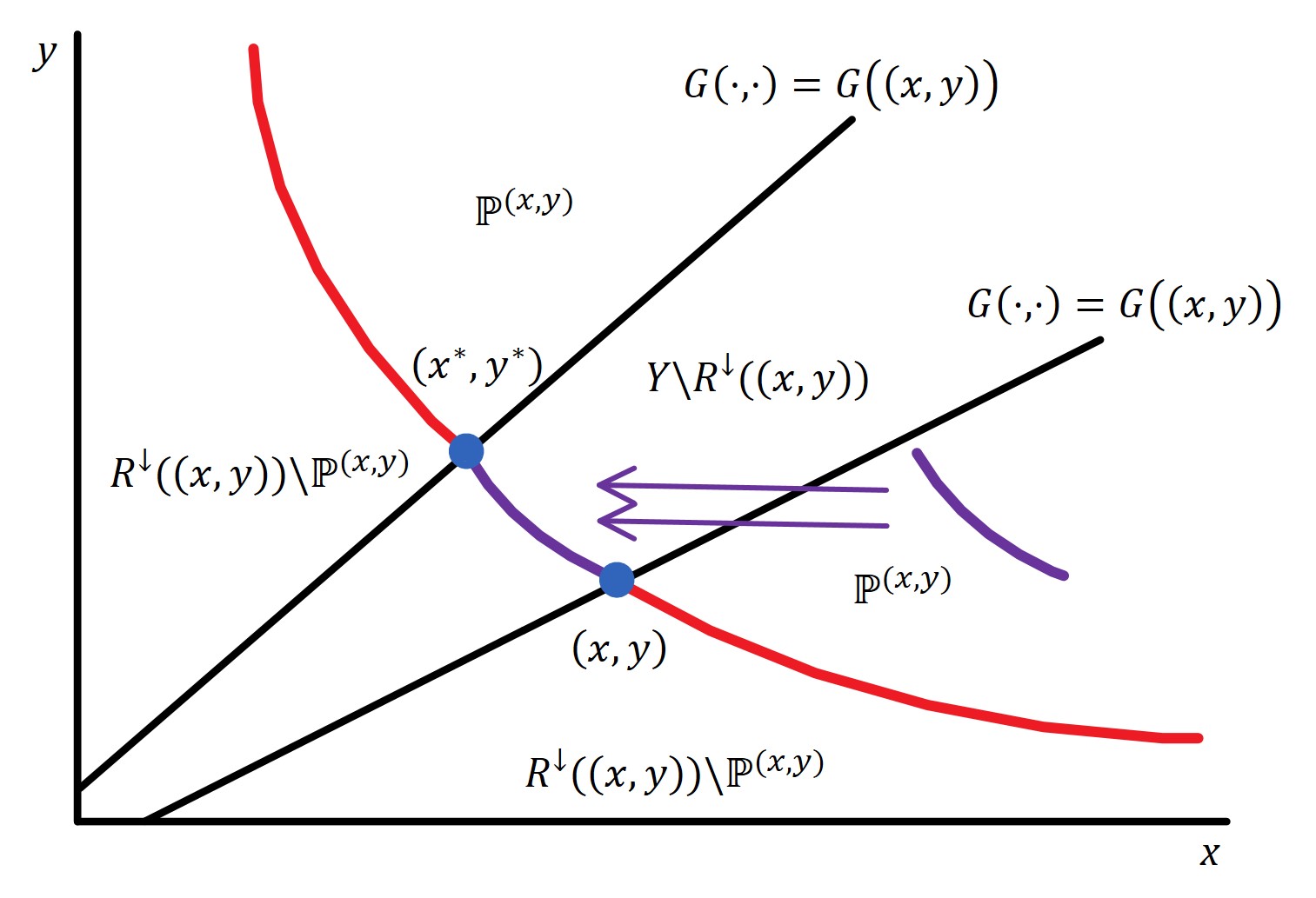
Figure B.1: This figure illustrates the construction of $v_{\left(x,y\right)}$ for a fixed $\left(x,y\right)\in Y$. The space $Y$ is divided into three regions: (1) Between the two diagonal lines are alternatives in $Y\backslash R^{\downarrow}\left(\left(x,y\right)\right)$, they have lower Gini coefficients than $\left(x,y\right)$, and therefore they appear in a choice problem where $\left(x,y\right)$ is the reference. The alternatives in $R^{\downarrow}\left(\left(x,y\right)\right)$ are then split into two groups: (2) those that are chosen when $\left(x,y\right)$ is the reference, $\mathbb{P}^{\left(x,y\right)}$, and (3) those that are not, $R^{\downarrow}\left(\left(x,y\right)\right)\backslash\mathbb{P}^{\left(x,y\right)}$. These two groups are separated by the indifference curve passing through $\left(x,y\right)$, the red curve, which partially constructs $v_{\left(x,y\right)}$ (partial because Gini coefficient truncates the space). The rest of $v_{\left(x,y\right)}$ can be constructed by using an indifference curve that connects $\left(x+a,y\right)$ and $\left(x^{*}+a,y^{*}\right)$, the purple curve, where $G\left(\left(x,y\right)\right)=G\left(\left(x^{*},y^{*}\right)\right)$, $c\left(\left\{\left(x,y\right),\left(x^{*},y^{*}\right)\right\}\right)=\left\{\left(x,y\right),\left(x^{*},y^{*}\right)\right\}$, and $\left(x+a,y\right),\left(x^{*}+a,y^{*}\right)\in\mathbb{P}^{\left(x,y\right)}$.

Stage 2: $x+\hat{v}_{g}\left(y\right)$ for each Gini coefficient $g$

Fix $g\in[0,0.5)$, we now show that $v_{\left(x,y\right)}$ must coincide for all $\left(x,y\right)$ where $G\left(\left(x,y\right)\right)=g$. Consider the collection of choice sets $\text{$\mathcal{S}$}:=\left\{A\in\mathcal{A}:\min_{z\in A}G\left(z\right)=g\right\}$. It turns out that $c$ satisfies WARP and Quasi-linearity over $\mathcal{S}$. To see this, take any two choice problems $A_{1},A_{2}$ in $\mathcal{S}$. For each $i=1,2$, there must be an alternative $\left(x_{i},y_{i}\right)\in A_{i}$ such that $G\left(\left(x_{i},y_{i}\right)\right)=g$ and $G\left(\left(x^{\prime},y^{\prime}\right)\right)\geq g$ for all other $\left(x^{\prime},y^{\prime}\right)$ in $A_{i}$. Consider an income distribution $\left(x^{*},y^{*}\right)$ such that $x^{*}\leq\min$$\left\{x_{1},x_{2}\right\}$ and $y^{*}\leq\min\left\{y_{1},y_{2}\right\}$ and $G\left(\left(x^{*},y^{*}\right)\right)=g$. Due to $\left(x_{i},y_{i}\right)\in\Psi\left(A_{i}\cup\left\{\left(x^{*},y^{*}\right)\right\}\right)$, 5.2, and 5.1, we have $c\left(A_{i}\right)=c\left(A_{i}\cup\left\{\left(x^{*},y^{*}\right)\right\}\right)$ for $i=1,2$. But $\left(x^{*},y^{*}\right)\in\Psi\left(A_{1}\cup A_{2}\cup\left\{\left(x^{*},y^{*}\right)\right\}\right)$, so by 5.2 again, between $c\left(A_{1}\cup\left\{\left(x^{*},y^{*}\right)\right\}\right)$ and $c\left(A_{2}\cup\left\{\left(x^{*},y^{*}\right)\right\}\right)$, which as established are equal to $c\left(A_{1}\right)$ and $c\left(A_{2}\right)$ respectively, WARP and Quasi-linearity must hold. Since $c$ satisfies WARP and Quasi-linearity over $\mathcal{S}$, there is a unique $\hat{v}_{g}:[w,+\infty)\rightarrow\mathbb{R}$ such that the utility function $\tilde{x}+\hat{v}_{g}\left(\tilde{y}\right)$ explains $\left(c,\mathcal{S}\right)$. But every $v_{\left(x,y\right)}$ constructed in Stage 1 is also unique, and $\mathbb{A}_{R^{\downarrow}\left(\left(x,y\right)\right)}^{\left(x,y\right)}\subseteq\mathcal{S}$ if $G\left(\left(x,y\right)\right)=g$, so $v_{\left(x,y\right)}$ must coincide for all $\left(x,y\right)$ such that $G\left(\left(x,y\right)\right)=g$.

Stage 3: $g<g^{\prime}$ implies $\hat{v}_{g}\left(y\right)-\hat{v}_{g}\left(y^{\prime}\right)\geq\hat{v}_{g^{\prime}}\left(y\right)-\hat{v}_{g^{\prime}}\left(y^{\prime}\right)$ for all $y>y^{\prime}$

Finally we show that the constructed $\hat{v}_{g}\left(y\right)^{\prime}s$ are systematically related. Consider any $g,g^{\prime}\in[0,0.5)$ such that $g<g^{\prime}$ (reminder: lower $g$ implies greater attainable equality) and any $y,y^{\prime}\in\mathbb{R}_{\geq 0}$ such that $y>y^{\prime}$. Define $\bar{v}_{g}:=\hat{v}_{g}\left(y\right)-\hat{v}_{g}\left(y^{\prime}\right)$ and $\bar{v}_{g^{\prime}}:=\hat{v}_{g^{\prime}}\left(y\right)-\hat{v}_{g^{\prime}}\left(y^{\prime}\right)$. We want to show $\bar{v}_{g}\geq\bar{v}_{g^{\prime}}$. Suppose not, our goal is to find a contradiction of 5.3 in choice behavior.

Let $z$ be a number such that $\bar{v}_{g}<z<\bar{v}_{g^{\prime}}$. Consider $\left(x_{g^{\prime}},w\right),\left(x_{g},w\right)\in Y$ such that $G\left(\left(x_{g^{\prime}},w\right)\right)=g^{\prime}$ and $G\left(\left(x_{g},w\right)\right)=g$, which exist because $G\left(\left(\tilde{x},w\right)\right)$ is continuous and increasing in $\tilde{x}$ from $G\left(\left(w,w\right)\right)=0$ to $\lim_{x\rightarrow+\infty}G\left(\left(x,w\right)\right)=0.5$ and $g,g^{\prime}\in[0,0.5)$. Consider $x:=z+\Delta$, $x^{\prime}:=2z+\Delta$ for some $\Delta>0$ such that $g^{\prime}\leq\min\left(\left\{G\left(\left(x,y\right)\right),G\left(\left(x^{\prime},y^{\prime}\right)\right)\right\}\right)$ and $x^{\prime}>x>\max\left(\left\{x_{g^{\prime}},x_{g}\right\}\right)$, where $\Delta$ exists because for any fixed $\bar{y}$, $G\left(\left(\tilde{x},\bar{y}\right)\right)$ is asymptotically increasing in $\tilde{x}$ and $\lim_{x\rightarrow+\infty}G\left(\left(x,\bar{y}\right)\right)=0.5$, and $g^{\prime}\in[0,0.5)$. Essentially, we have introduced reference points $\left(x_{g^{\prime}},w\right),\left(x_{g},w\right)$ that will not be chosen (due in part to 5.1), forcing the choice to be between $\left(x,y\right)$ and $\left(x^{\prime},y^{\prime}\right)$.

We now use the constructed alternatives, $\left(x,y\right),\left(x^{\prime},y^{\prime}\right),\left(x_{g^{\prime}},w\right),\left(x_{g},w\right)$, to demonstrate a violation of 5.3. For the choice problem $\left\{\left(x,y\right),\left(x^{\prime},y^{\prime}\right),\left(x_{g^{\prime}},w\right)\right\}$, $\left(x_{g^{\prime}},w\right)$ is the reference (so $\hat{v}_{g^{\prime}}$ is used) and cannot be chosen. Since $\bar{v}_{g^{\prime}}>z$, or equivalently $z+\hat{v}_{g^{\prime}}\left(y\right)>2z+\hat{v}_{g^{\prime}}\left(y^{\prime}\right)$, we have $x+\hat{v}_{g^{\prime}}\left(y\right)>x^{\prime}+\hat{v}_{g^{\prime}}\left(y^{\prime}\right)$, and therefore

$$c\left(\left\{\left(x,y\right),\left(x^{\prime},y^{\prime}\right),\left(x_{g^{\prime}},w\right)\right\}\right)=\left\{\left(x,y\right)\right\}.$$ (B.2)

By analogous arguments, $z>\bar{v}_{g}$ gives $c\left(\left\{\left(x,y\right),\left(x^{\prime},y^{\prime}\right),\left(x_{g},w\right)\right\}\right)=\left\{\left(x^{\prime},y^{\prime}\right)\right\}$ ($\hat{v}_{g}$ is used), which also gives

$$c\left(\left\{\left(x,y\right),\left(x^{\prime},y^{\prime}\right),\left(x_{g^{\prime}},w\right),\left(x_{g},w\right)\right\}\right)=\left\{\left(x^{\prime},y^{\prime}\right)\right\}.$$ (B.3)

due to 5.2 and $G\left(\left(x_{g},w\right)\right)=g\leq g^{\prime}=G\left(\left(x_{g^{\prime}},w\right)\right)$. Since $y>y^{\prime}$, (LABEL:fspu_increasing_v_4) and (LABEL:fspu_increasing_v_5) jointly contradict 5.3.

Stage 4: $R$ on $Y$

Create a complete, transitive, and antisymmetric $R$ on $Y$ such that $G\left(\left(x,y\right)\right)<G\left(\left(x^{\prime},y^{\prime}\right)\right)$ implies $\left(x,y\right)R\left(x^{\prime},y^{\prime}\right)$, which involves an arbitrary completion when $G\left(\left(x,y\right)\right)=G\left(\left(x^{\prime},y^{\prime}\right)\right)$.

B.6 Proof of Propositions 1, 2, 3

I focus on showing that WARP (1) and structural postulate (2) are independently sufficient for the standard model (3). The remaining statements, that WARP and structural postulates are necessary for standard models ((1) if (3) and (2) if (3)), and that WARP is sufficient and necessary for a (general) utility representation ((1) if and only if (4)), are well-known and omitted.

Proof of 1: (1) / (2) implies (3)

Suppose a choice correspondence $c$ admits an AREU representation with specification $\left(R,\left\{u_{r}\right\}_{r}\right)$. Suppose $c$ satisfies WARP or Independence (or both). We first show that $u_{r}=u_{s}$ for all $r,s\in\Delta\left(X\right)\backslash\text{conv}\left(\left\{\delta_{b},\delta_{w}\right\}\right)$. Suppose without loss of generality $rRs$. Suppose for contradiction $u_{r}\neq u_{s}$, then the fact that $u_{r}$ is a concave transformation of $u_{s}$ and that both functions are normalized to $\left[0,1\right]$ implies $u_{r}\left(x\right)>u_{s}\left(x\right)$ for all $x\in X\backslash\left\{b,w\right\}$. Consider the set $\tau_{s}:=\text{conv}\left(\left\{s,\delta_{b},\delta_{w}\right\}\right)$. The interior of this set, $\text{Int}\tau_{s}$, consists of lotteries that are extreme spreads of $s$, hence $\text{Int}\tau_{s}\subseteq R^{\downarrow}\left(s\right)\subseteq R^{\downarrow}\left(r\right)$. By 3.1, $c\left(\left\{\delta_{b},r\right\}\right)=c\left(\left\{\delta_{b},s\right\}\right)=\delta_{b}$. Then by Continuity, there exist open balls around $\delta_{b}$, $B_{r}$ and $B_{s}$, such that they contain lotteries that are chosen over $r$ and $s$ respectively. Now consider an open subset $S$ of $B_{r}\cap B_{s}\cap\text{Int}\tau_{s}$. Since $u_{r}\left(x\right)>u_{s}\left(x\right)$ for all $x\in X\backslash\left\{b,w\right\}$, we can find lotteries $p,q\in S$ such that $\mathbb{E}_{p}u_{r}\left(x\right)>\mathbb{E}_{q}u_{r}\left(x\right)$ and $\mathbb{E}_{p}u_{s}\left(x\right)<\mathbb{E}_{q}u_{s}\left(x\right)$. This means

$$c\left(\left\{r,s,p,q\right\}\right) =\left\{p\right\}\text{ and}$$ (B.4)

$$c\left(\left\{s,p,q\right\}\right) =\left\{q\right\}.$$ (B.5)

Consider $t\in S$, $p^{\prime}=\frac{1}{2}p\oplus\frac{1}{2}t$, and $q^{\prime}=\frac{1}{2}q\oplus\frac{1}{2}t$, then $p^{\prime},q^{\prime}\in S$, and therefore

$$c\left(\left\{s,p^{\prime},q^{\prime}\right\}\right)=\left\{q^{\prime}\right\}.$$ (B.6)

Finally we conclude that (LABEL:warp1_1) and (LABEL:warp1_2) jointly violate WARP, whereas (LABEL:warp1_1) and (LABEL:warp1_3) jointly violate Independence.

Next we turn to $r\in\text{conv}\left(\left\{\delta_{b},\delta_{w}\right\}\right)$ and show that $u_{r}$ is either identical, or has the freedom to be identical, to $u_{s}$ where $s\in\Delta\left(X\right)\backslash\text{conv}\left(\left\{\delta_{b},\delta_{w}\right\}\right)$. If $r=\delta_{b}$ or $r=\delta_{w}$ or $R^{\downarrow}\left(r\right)\subseteq\text{conv}\left(\left\{\delta_{b},\delta_{w}\right\}\right)$, then any strictly increasing $u_{r}$ can explain $c$ over $\mathbb{A}_{R^{\downarrow}\left(r\right)}^{r}:=\left\{A\in\mathcal{A}:A\subseteq R^{\downarrow}\left(r\right)\text{ and }r\in A\right\}$, so we can just pick one that is identical to $u_{s}$ for every $s\in\Delta\left(X\right)\backslash\text{conv}\left(\left\{\delta_{b},\delta_{w}\right\}\right)$. If $r$ doesn’t satisfy any of those conditions, then there exists $s_{2}\in\Delta\left(X\right)\backslash\text{conv}\left(\left\{\delta_{b},\delta_{w}\right\}\right)$ such that $r$ is an extreme spread of $s_{2}$ and there exists $s_{1}\in R^{\downarrow}\left(r\right)\backslash\text{conv}\left(\left\{\delta_{b},\delta_{w}\right\}\right)$. This implies $u_{s_{2}}$ is a concave transformation of $u_{r}$ (because $s_{2}Rr$) and $u_{r}$ is a concave transformation of $u_{s_{1}}$ (because $rRs_{1}$), but we already showed that $u_{s_{1}}=u_{s_{2}}$ (since $s_{1},s_{2}\in\Delta\left(X\right)\backslash\text{conv}\left(\left\{\delta_{b},\delta_{w}\right\}\right))$, so $u_{r}$ is identical to $u_{s}$ for all $s\in\Delta\left(X\right)\backslash\text{conv}\left(\left\{\delta_{b},\delta_{w}\right\}\right)$. We conclude that if either WARP or Independence (or both) holds, then $c$ admits an expected utility representation.

Proof of 2: (1) / (2) implies (3)

Suppose a choice correspondence $c$ admits a PEDU representation with specification $\left(\left\{\delta_{r}\right\}_{r},u\right)$. We show that if $\delta_{r}\neq\delta_{r^{\prime}}$ for some $r,r^{\prime}\in[0,\bar{t})$, then $c$ violates both WARP and Stationarity. ($\delta_{\bar{t}}$ only plays a role for choice problems $A\in\mathcal{A}$ where every alternative has $t=\bar{t}$, so we set it as $\delta_{\bar{t}}=\delta_{0}$.)

Suppose for contradiction $\delta_{r}\neq\delta_{r^{\prime}}$ for some $r,r^{\prime}\in[0,\bar{t})$. Say without loss of generality $r>r^{\prime}\geq 0$, then $\delta_{r}>\delta_{r^{\prime}}\geq\delta_{0}$. Recall that $X=\left[a,b\right]$. Consider alternatives $\left(b-\Delta_{x},0\right),\left(b,0+\Delta_{t}\right)\in X\times T$ such that (i) $\Delta_{x}\in\left(0,b-a\right)$, (ii) $\Delta_{t}\in\left(0,\bar{t}-r\right)$, (iii) $\delta_{r}^{0}u\left(b-\Delta_{x}\right)<\delta_{r}^{0+\Delta_{t}}u\left(b\right)$, and (iv) $\delta_{0}^{0}u\left(b-\Delta_{x}\right)>\delta_{0}^{0+\Delta_{t}}u\left(b\right)$, which is possible due in part to the assumption that $\left(b,\bar{t}\right)\in c\left(\left\{\left(a,0\right),\left(b,\bar{t}\right)\right\}\right)$. Note that (i) and (ii) guarantee $\left(b-\Delta_{x},0\right),\left(b,0+\Delta_{t}\right),\left(b-\Delta_{x},r\right),\left(b,r+\Delta_{t}\right)\in X\times T$. Then, (iii) gives

$$c\left(\left\{\left(b-\Delta_{x},r\right),\left(b,r+\Delta_{t}\right)\right\}\right)=\left\{\left(b,r+\Delta_{t}\right)\right\},$$ (B.7)

and (iv) gives

$$c\left(\left\{\left(b-\Delta_{x},0\right),\left(b,0+\Delta_{t}\right)\right\}\right) =\left\{\left(b-\Delta_{x},0\right)\right\}\text{ and}$$ (B.8)

$$c\left(\left\{\left(a,0\right),\left(b-\Delta_{x},r\right),\left(b,r+\Delta_{t}\right)\right\}\right) =\left\{\left(b-\Delta_{x},r\right)\right\},$$ (B.9)

where (LABEL:warp2_7) is due in part to the assumption that $\left(b,\bar{t}\right)\in c\left(\left\{\left(a,0\right),\left(b,\bar{t}\right)\right\}\right)$ as it excludes $\left(a,0\right)$ from being uniquely chosen. Now note that (LABEL:warp2_5) and (LABEL:warp2_6) jointly violate Stationarity, whereas (LABEL:warp2_5) and (LABEL:warp2_7) jointly violate WARP. We conclude that if either WARP or Stationarity (or both) holds, then $c$ admits an exponential discounting utility representation.

Proof of 3: (1) / (2) implies (3)

Suppose a choice correspondence $c$ admits an FSPU representation with specification $\left\{v_{r}\right\}_{r}$. We show that if $v_{r}\left(y\right)-v_{r}\left(y^{\prime}\right)\neq v_{r^{\prime}}\left(y\right)-v_{r^{\prime}}\left(y^{\prime}\right)$ for some $r,r^{\prime}$ and $y>y^{\prime}$, then $c$ violates both WARP and Quasi-linearity.

Suppose for contradiction $v_{r}\left(y\right)-v_{r}\left(y^{\prime}\right)\neq v_{r^{\prime}}\left(y\right)-v_{r^{\prime}}\left(y^{\prime}\right)$ for some $r,r^{\prime}\in[0,0.5)$ and $y>y^{\prime}$. Without loss of generality, say $r>r^{\prime}\geq 0$. Then $v_{r}\left(y\right)-v_{r}\left(y^{\prime}\right)<v_{r^{\prime}}\left(y\right)-v_{r^{\prime}}\left(y^{\prime}\right)\leq v_{0}\left(y\right)-v_{0}\left(y^{\prime}\right)$, and therefore there exist $\tilde{x},\tilde{x}^{\prime}\in[w,+\infty)$ such that $\tilde{x}^{\prime}+v_{r}\left(y^{\prime}\right)>\tilde{x}+v_{r}\left(y\right)$ and $\tilde{x}^{\prime}+v_{0}\left(y^{\prime}\right)<\tilde{x}+v_{0}\left(y\right)$. Consider $\left(x^{*},y^{*}\right)\in Y$ such that $y^{*}=w$ and $G\left(\left(x^{*},y^{*}\right)\right)=r$, which is possible since $G\left(\left(\cdot,w\right)\right)$ is continuous and increasing in it’s first argument from $G\left(\left(w,w\right)\right)=0$ to $\lim_{x\rightarrow+\infty}G\left(\left(x,w\right)\right)=0.5$. Since for any fixed $\bar{y}$, $G\left(\left(\cdot,\bar{y}\right)\right)$ is asymptotically increasing in it’s first argument, there exists $\Delta>0$ such that $\min\left(\left\{G\left(\left(\tilde{x}+\Delta,y\right)\right),G\left(\left(\tilde{x}^{\prime}+\Delta,y^{\prime}\right)\right)\right\}\right)\geq r$ and $\min\left(\left\{\tilde{x}+\Delta,\tilde{x}^{\prime}+\Delta\right\}\right)>x^{*}$. Let $x:=\tilde{x}+\Delta$ and $x^{\prime}:=\tilde{x}^{\prime}+\Delta$. We have now established that (i) $\min\left(\left\{x,x^{\prime}\right\}\right)>x^{*}\geq w,\min\left(\left\{y,y^{\prime}\right\}\right)\geq y^{*}=w$, (ii) $\min\left(\left\{G\left(\left(x,y\right)\right),G\left(\left(x^{\prime},y^{\prime}\right)\right)\right\}\right)\geq G\left(\left(x^{*},y^{*}\right)\right)=r$, (iii) $x^{\prime}+v_{r}\left(y^{\prime}\right)>x+v_{r}\left(y\right)$, and (iv) $x^{\prime}+v_{0}\left(y^{\prime}\right)<x+v_{0}\left(y\right)$.

Then, (i), (ii), and (iii) together give

$$c\left(\left\{\left(x^{*},y^{*}\right),\left(x,y\right),\left(x^{\prime},y^{\prime}\right)\right\}\right) =\left\{\left(x^{\prime},y^{\prime}\right)\right\},$$ (B.10)

whereas (i) and (iv) together give

$$c\left(\left\{\left(w,w\right),\left(x,y\right),\left(x^{\prime},y^{\prime}\right)\right\}\right) =\left\{\left(x,y\right)\right\}\text{ and}$$ (B.11)

$$c\left(\left\{\left(w,w\right),\left(x+\epsilon,y\right),\left(x^{\prime}+\epsilon,y^{\prime}\right)\right\}\right) =\left\{\left(x+\epsilon,y\right)\right\}\,\forall\epsilon>0.$$ (B.12)

Note that (LABEL:warp3_3) and (LABEL:warp3_5) jointly violate Quasi-linearity. Separately, by WARP, (LABEL:warp3_3) and (LABEL:warp3_4) imply $c\left(\left\{\left(x,y\right),\left(x^{\prime},y^{\prime}\right)\right\}\right)=\left\{\left(x^{\prime},y^{\prime}\right)\right\}$ and $c\left(\left\{\left(x,y\right),\left(x^{\prime},y^{\prime}\right)\right\}\right)=\left\{\left(x,y\right)\right\}$ respectively, which is also a contradiction. We conclude that if either WARP or Quasi-linearity (or both) holds, then $c$ admits a quasi-linear utility representation.

References

- (1)
- Ahn, Iijima, Le Yaouanq, and Sarver (2019) Ahn, D. S., R. Iijima, Y. Le Yaouanq, and T. Sarver (2019): “Behavioural Characterizations of Naivete for Time-inconsistent Preferences,” The Review of Economic Studies, 86(6), 2319–2355.
- Ainslie (1992) Ainslie, G. (1992): Picoeconomics: The Strategic Interaction of Successive Motivational States within the Person. Cambridge University Press.
- Allais (1990) Allais, M. (1990): “Allais Paradox,” in Utility and Probability, pp. 3–9. Springer.
- Andreoni and Sprenger (2011) Andreoni, J., and C. Sprenger (2011): “Uncertainty Equivalents: Testing the Limits of the Independence Axiom,” Working paper, National Bureau of Economic Research.
- Apesteguia and Ballester (2009) Apesteguia, J., and M. A. Ballester (2009): “A Theory of Reference-Dependent Behavior,” Economic Theory, 40, 427–455.
- Aumann (1962) Aumann, R. J. (1962): “Utility Theory without the Completeness Axiom,” Econometrica, pp. 445–462.
- Aumann and Serrano (2008) Aumann, R. J., and R. Serrano (2008): “An Economic Index of Riskiness,” Journal of Political Economy, 116(5), 810–836.
- Bardsley (2008) Bardsley, N. (2008): “Dictator Game Giving: Altruism or Artefact?,” Experimental Economics, 11(2), 122–133.
- Benhabib, Bisin, and Schotter (2010) Benhabib, J., A. Bisin, and A. Schotter (2010): “Present-Bias, Quasi-Hyperbolic Discounting, and Fixed Costs,” Games and Economic Behavior, 69(2), 205–223.
- Bleichrodt and Schmidt (2002) Bleichrodt, H., and U. Schmidt (2002): “A Context-Dependent Model of the Gambling Effect,” Management Science, 48(6), 802–812.
- Bolton and Ockenfels (2000) Bolton, G. E., and A. Ockenfels (2000): “ERC: A Theory of Equity, Reciprocity, and Competition,” American Economic Review, 90(1), 166–193.
- Bordalo, Gennaioli, and Shleifer (2012) Bordalo, P., N. Gennaioli, and A. Shleifer (2012): “Salience Theory of Choice under Risk,” Quarterly Journal of Economics, 127(3), 1243–1285.
- Bordalo, Gennaioli, and Shleifer (2013) (2013): “Salience and Consumer Choice,” Journal of Political Economy, 121(5), 803–843.
- Burks, Carpenter, Goette, and Rustichini (2009) Burks, S. V., J. P. Carpenter, L. Goette, and A. Rustichini (2009): “Cognitive Skills Affect Economic Preferences, Strategic Behavior, and Job Attachment,” Proceedings of the National Academy of Sciences, 106(19), 7745–7750.
- Cerreia-Vioglio, Dillenberger, and Ortoleva (2015) Cerreia-Vioglio, S., D. Dillenberger, and P. Ortoleva (2015): “Cautious Expected Utility and the Certainty Effect,” Econometrica, 83(2), 693–728.
- Chakraborty (2021) Chakraborty, A. (2021): “Present Bias,” Econometrica, 89(4), 1921–1961.
- Chakraborty, Halevy, and Saito (2020) Chakraborty, A., Y. Halevy, and K. Saito (2020): “The Relation between Behavior under Risk and over Time,” American Economic Review: Insights, 2(1), 1–16.
- Chambers, Echenique, and Miller (2023) Chambers, C. P., F. Echenique, and A. D. Miller (2023): “Decreasing Impatience,” American Economic Journal: Microeconomics, 15(3), 527–551.
- Chapman, Dean, Ortoleva, Snowberg, and Camerer (2023) Chapman, J., M. Dean, P. Ortoleva, E. Snowberg, and C. Camerer (2023): “Econographics,” Journal of Political Economy Microeconomics, 1(1), 115–161.
- Charness and Rabin (2002) Charness, G., and M. Rabin (2002): “Understanding Social Preferences with Simple Tests,” Quarterly Journal of Economics, 117(3), 817–869.
- Chen, Liu, Shan, Zhong, and Zhou (2023) Chen, M., T. X. Liu, Y. Shan, S. Zhong, and Y. Zhou (2023): “The Consistency of Rationality Measures,” Unpublished.
- Cheung (2023) Cheung, P. H. Y. (2023): “Revealed Reciprocity,” Unpublished.
- Chew (1983) Chew, S. H. (1983): “A Generalization of the Quasilinear Mean with Applications to the Measurement of Income Inequality and Decision Theory Resolving the Allais Paradox,” Econometrica, 51(4), 1065–1092.
- Cox, Friedman, and Sadiraj (2008) Cox, J. C., D. Friedman, and V. Sadiraj (2008): “Revealed Altruism,” Econometrica, 76(1), 31–69.
- Cox, List, Price, Sadiraj, and Samek (2016) Cox, J. C., J. A. List, M. Price, V. Sadiraj, and A. Samek (2016): “Moral Costs and Rational Choice: Theory and Experimental Evidence,” Working paper, National Bureau of Economic Research.
- Dana, Cain, and Dawes (2006) Dana, J., D. M. Cain, and R. M. Dawes (2006): “What You Don’t Know Won’t Hurt Me: Costly (But Quiet) Exit in Dictator Games,” Organizational Behavior and Human Decision Processes, 100(2), 193–201.
- Dana, Weber, and Kuang (2007) Dana, J., R. A. Weber, and J. X. Kuang (2007): “Exploiting Moral Wiggle Room: Experiments Demonstrating an Illusory Preference for Fairness,” Economic Theory, 33(1), 67–80.
- de Clippel and Rozen (2021) de Clippel, G., and K. Rozen (2021): “Bounded Rationality and Limited Data Sets,” Theoretical Economics, 16(2), 359–380.
- de Clippel and Rozen (2023) (2023): “Relaxed Optimization: How Close Is a Consumer to Satisfying First-Order Conditions?,” Review of Economics and Statistics, 105(4), 883–898.
- Dean, Kıbrıs, and Masatlioglu (2017) Dean, M., Ö. Kıbrıs, and Y. Masatlioglu (2017): “Limited Attention and Status Quo Bias,” Journal of Economic Theory, 169, 93–127.
- Dean and Ortoleva (2019) Dean, M., and P. Ortoleva (2019): “The Empirical Relationship between Nonstandard Economic Behaviors,” Proceedings of the National Academy of Sciences, 116(33), 16262–16267.
- Dekel (1986) Dekel, E. (1986): “An Axiomatic Characterization of Preferences under Uncertainty: Weakening the Independence Axiom,” Journal of Economic Theory, 40(2), 304–318.
- Dembo, Kariv, Polisson, and Quah (2021) Dembo, A., S. Kariv, M. Polisson, and J. Quah (2021): “Ever Since Allais,” Bristol Economics Discussion Papers, 21/745.
- Dillenberger (2010) Dillenberger, D. (2010): “Preferences for One-Shot Resolution of Uncertainty and Allais-Type Behavior,” Econometrica, 78(6), 1973–2004.
- Dillenberger and Sadowski (2012) Dillenberger, D., and P. Sadowski (2012): “Ashamed to be Selfish,” Theoretical Economics, 7(1), 99–124.
- Dubra, Maccheroni, and Ok (2004) Dubra, J., F. Maccheroni, and E. A. Ok (2004): “Expected Utility Theory Without the Completeness Axiom,” Journal of Economic Theory, 115(1), 118–133.
- Echenique, Imai, and Saito (2020) Echenique, F., T. Imai, and K. Saito (2020): “Testable Implications of Models of Intertemporal Choice: Exponential Discounting and its Generalizations,” American Economic Journal: Microeconomics, 12(4), 114–143.
- Echenique, Imai, and Saito (2023) (2023): “Approximate Expected Utility Rationalization,” Journal of the European Economic Association, p. jvad028.
- Ellis and Masatlioglu (2022) Ellis, A., and Y. Masatlioglu (2022): “Choice with Endogenous Categorization,” Review of Economic Studies, 89(1), 240–278.
- Evren (2014) Evren, Ö. (2014): “Scalarization Methods and Expected Multi-Utility Representations,” Journal of Economic Theory, 151, 30–63.
- Falk, Becker, Dohmen, Enke, Huffman, and Sunde (2018) Falk, A., A. Becker, T. Dohmen, B. Enke, D. Huffman, and U. Sunde (2018): “Global Evidence on Economic Preferences,” Quarterly Journal of Economics, 133(4), 1645–1692.
- Fehr and Schmidt (1999) Fehr, E., and K. M. Schmidt (1999): “A Theory of Fairness, Competition, and Cooperation,” Quarterly Journal of Economics, 114(3), 817–868.
- Fehr and Schmidt (2006) (2006): “The Economics of Fairness, Reciprocity and Altruism: Experimental Evidence and New Theories,” Handbook of the Economics of Giving, Altruism and Reciprocity, 1, 615–691.
- Fishburn (1983) Fishburn, P. C. (1983): “Transitive Measurable Utility,” Journal of Economic Theory, 31(2), 293–317.
- Fishburn and Rubinstein (1982) Fishburn, P. C., and A. Rubinstein (1982): “Time Preference,” International Economic Review, 23(3), 677–694.
- Frederick, Loewenstein, and O’donoghue (2002) Frederick, S., G. Loewenstein, and T. O’donoghue (2002): “Time Discounting and Time Preference: A Critical Review,” Journal of Economic Literature, 40(2), 351–401.
- Freeman (2017) Freeman, D. J. (2017): “Preferred Personal Equilibrium and Simple Choices,” Journal of Economic Behavior & Organization, 143, 165–172.
- Freeman (2021) Freeman, D. J. (2021): “Revealing Naïveté and Sophistication from Procrastination and Preproperation,” American Economic Journal: Microeconomics, 13(2), 402–38.
- Giarlotta, Petralia, and Watson (2023) Giarlotta, A., A. Petralia, and S. Watson (2023): “Context-Sensitive Rationality: Choice by Salience,” Journal of Mathematical Economics, 109, 102913.
- Gilboa and Schmeidler (1989) Gilboa, I., and D. Schmeidler (1989): “Maxmin Expected Utility with Non-Unique Prior,” Journal of Mathematical Economics, 18(2), 141–153.
- Gul (1991) Gul, F. (1991): “A Theory of Disappointment Aversion,” Econometrica, 59(3), 667–686.
- Gul and Pesendorfer (2001) Gul, F., and W. Pesendorfer (2001): “Temptation and Self-Control,” Econometrica, 69(6), 1403–1435.
- Halevy (2015) Halevy, Y. (2015): “Time Consistency: Stationarity and Time Invariance,” Econometrica, 83(1), 335–352.
- Halevy, Walker-Jones, and Zrill (2023) Halevy, Y., D. Walker-Jones, and L. Zrill (2023): “Difficult Decisions,” Working papers, University of Toronto, Department of Economics.
- Hara, Ok, and Riella (2019) Hara, K., E. A. Ok, and G. Riella (2019): “Coalitional Expected Multi-Utility Theory,” Econometrica, 87(3), 933–980.
- Herne (1999) Herne, K. (1999): “The Effects of Decoy Gambles on Individual Choice,” Experimental Economics, 2(1), 31–40.
- Houthakker (1950) Houthakker, H. S. (1950): “Revealed Preference and the Utility Function,” Economica, 17(66), 159–174.
- Huber, Payne, and Puto (1982) Huber, J., J. W. Payne, and C. Puto (1982): “Adding Asymmetrically Dominated Alternatives: Violations of Regularity and the Similarity Hypothesis,” Journal of Consumer Research, 9(1), 90–98.
- Kagel and Roth (2016) Kagel, J. H., and A. E. Roth (2016): The Handbook of Experimental Economics, vol. 1. Princeton University Press.
- Kahneman, Knetsch, and Thaler (1991) Kahneman, D., J. L. Knetsch, and R. H. Thaler (1991): “Anomalies: The Endowment Effect, Loss Aversion, and Status Quo Bias,” Journal of Economic Perspectives, 5(1), 193–206.
- Kahneman and Tversky (1979) Kahneman, D., and A. Tversky (1979): “Prospect Theory: An Analysis of Choice under Risk,” Econometrica, 47(2), 263–292.
- Ke and Chen (2022) Ke, S., and Z. Chen (2022): “From Local Utility to Neural Networks,” Unpublished.
- Kıbrıs, Masatlioglu, and Suleymanov (2023) Kıbrıs, Ö., Y. Masatlioglu, and E. Suleymanov (2023): “A Theory of Reference Point Formation,” Economic Theory, 75, 137–166.
- Kibris, Masatlioglu, and Suleymanov (2024) Kibris, Ã., Y. Masatlioglu, and E. Suleymanov (2024): “A Random Reference Model,” American Economic Journal: Microeconomics, 16(1), 155–209.
- Kivetz, Netzer, and Srinivasan (2004) Kivetz, R., O. Netzer, and V. Srinivasan (2004): “Alternative Models for Capturing the Compromise Effect,” Journal of Marketing Research, 41(3), 237–257.
- Koopmans (1960) Koopmans, T. C. (1960): “Stationary Ordinal Utility and Impatience,” Econometrica, 28(2), 287–309.
- Korenok, Millner, and Razzolini (2014) Korenok, O., E. L. Millner, and L. Razzolini (2014): “Taking, Giving, and Impure Altruism in Dictator Games,” Experimental Economics, 17(3), 488–500.
- Kőszegi and Rabin (2006) Kőszegi, B., and M. Rabin (2006): “A Model of Reference-Dependent Preferences,” Quarterly Journal of Economics, 121(4), 1133–1165.
- Kőszegi and Rabin (2007) (2007): “Reference-Dependent Risk Attitudes,” American Economic Review, 97(4), 1047–1073.
- Kőszegi and Szeidl (2013) Kőszegi, B., and A. Szeidl (2013): “A Model of Focusing in Economic Choice,” Quarterly Journal of Economics, 128(1), 53–104.
- Kovach (2020) Kovach, M. (2020): “Twisting the Truth: Foundations of Wishful Thinking,” Theoretical Economics, 15(3), 989–1022.
- Laibson (1997) Laibson, D. (1997): “Golden Eggs and Hyperbolic Discounting,” Quarterly Journal of Economics, 112(2), 443–478.
- Lanzani (2022) Lanzani, G. (2022): “Correlation Made Simple: Applications to Salience and Regret Theory,” The Quarterly Journal of Economics, 137(2), 959–987.
- Lim (2023a) Lim, X. Z. (2023a): “An Analysis of Avoidable Risk Expected Utility,” Unpublished.
- Lim (2023b) (2023b): “An Analysis of Ordered Reference Dependent Utility,” Unpublished.
- Lipman, Pesendorfer, et al. (2013) Lipman, B. L., W. Pesendorfer, et al. (2013): “Temptation,” in Advances in economics and econometrics: Tenth World Congress, vol. 1, pp. 243–288. Cambridge University Press.
- List (2007) List, J. A. (2007): “On the Interpretation of Giving in Dictator Games,” Journal of Political Economy, 115(3), 482–493.
- Loewenstein and Prelec (1992) Loewenstein, G., and D. Prelec (1992): “Anomalies in Intertemporal Choice: Evidence and an Interpretation,” Quarterly Journal of Economics, 107(2), 573–597.
- Machina (1982) Machina, M. J. (1982): “‘Expected Utility’ Analysis without the Independence Axiom,” Econometrica, 50(2), 277–323.
- Manzini and Mariotti (2008) Manzini, P., and M. Mariotti (2008): “On the Representation of Incomplete Preferences over Risky Alternatives,” Theory and Decision, 65, 303–323.
- Masatlioglu and Ok (2005) Masatlioglu, Y., and E. A. Ok (2005): “Rational Choice with Status Quo Bias,” Journal of Economic Theory, 121(1), 1–29.
- Masatlioglu and Ok (2014) (2014): “A Canonical Model of Choice with Initial Endowments,” Review of Economic Studies, 81(2), 851–883.
- Nelson (2002) Nelson, Jr., W. R. (2002): “Equity or Intention: It is the Thought that Counts,” Journal of Economic Behavior & Organization, 48(4), 423–430.
- Nielsen and Rehbeck (2022) Nielsen, K., and J. Rehbeck (2022): “When Choices are Mistakes,” American Economic Review, 112(7), 2237–2268.
- Noor (2011) Noor, J. (2011): “Temptation and Revealed Preference,” Econometrica, 79(2), 601–644.
- Noor and Takeoka (2015) Noor, J., and N. Takeoka (2015): “Menu-dependent Self-control,” Journal of Mathematical Economics, 61, 1–20.
- Ok and Benoît (2007) Ok, E. A., and J.-P. Benoît (2007): “Delay Aversion,” Theoretical Economics, 2(1), 71–113.
- Ok, Ortoleva, and Riella (2015) Ok, E. A., P. Ortoleva, and G. Riella (2015): “Revealed (P)Reference Theory,” American Economic Review, 105(1), 299–321.
- Orhun (2009) Orhun, A. Y. (2009): “Optimal Product Line Design when Consumers Exhibit Choice Set-Dependent Preferences,” Marketing Science, 28(5), 868–886.
- Ortoleva (2010) Ortoleva, P. (2010): “Status Quo Bias, Multiple Priors and Uncertainty Aversion,” Games and Economic Behavior, 69(2), 411–424.
- Phelps and Pollak (1968) Phelps, E. S., and R. A. Pollak (1968): “On Second-best National Saving and Game-equilibrium Growth,” Review of Economic Studies, 35(2), 185–199.
- Polisson, Quah, and Renou (2020) Polisson, M., J. K.-H. Quah, and L. Renou (2020): “Revealed Preferences over Risk and Uncertainty,” American Economic Review, 110(6), 1782–1820.
- Quiggin (1982) Quiggin, J. (1982): “A Theory of Anticipated Utility,” Journal of Economic Behavior & Organization, 3(4), 323–343.
- Rabin (1993) Rabin, M. (1993): “Incorporating Fairness into Game Theory and Economics,” American Economic Review, 83(5), 1281–1302.
- Ravid and Steverson (2021) Ravid, D., and K. Steverson (2021): “Bad Temptation,” Journal of Mathematical Economics, 95, 102480.
- Rubinstein and Salant (2006) Rubinstein, A., and Y. Salant (2006): “Two Comments on the Principle of Revealed Preference,” Unpublished.
- Rubinstein and Zhou (1999) Rubinstein, A., and L. Zhou (1999): “Choice Problems with a ’Reference’ Point,” Mathematical Social Sciences, 37(3), 205–209.
- Sagi (2006) Sagi, J. S. (2006): “Anchored Preference Relations,” Journal of Economic Theory, 130(1), 283–295.
- Samuelson (1948) Samuelson, P. A. (1948): “Consumption Theory in Terms of Revealed Preference,” Economica, 15(60), 243–253.
- Simonson (1989) Simonson, I. (1989): “Choice Based on Reasons: The Case of Attraction and Compromise Effects,” Journal of Consumer Research, 16(2), 158–174.
- Stango and Zinman (2023) Stango, V., and J. Zinman (2023): “We Are All Behavioural, More, or Less: A Taxonomy of Consumer Decision-Making,” Review of Economic Studies, 90(3), 1470–1498.
- Sutter (2007) Sutter, M. (2007): “Outcomes versus Intentions: On the Nature of Fair Behavior and its Development with Age,” Journal of Economic Psychology, 28(1), 69–78.
- Tserenjigmid (2019) Tserenjigmid, G. (2019): “Choosing with the Worst in Mind: A Reference-Dependent Model,” Journal of Economic Behavior & Organization, 157, 631–652.
- Tversky and Kahneman (1991) Tversky, A., and D. Kahneman (1991): “Loss Aversion in Riskless Choice: A Reference-Dependent Model,” Quarterly Journal of Economics, 106(4), 1039–1061.
- van Bruggen, Heufer, and Yang (2023) van Bruggen, P., J. Heufer, and J. Yang (2023): “Giving According to Agreement,” Unpublished.
- Wakker and Deneffe (1996) Wakker, P., and D. Deneffe (1996): “Eliciting von Neumann-Morgenstern Utilities when Probabilities are Distorted or Unknown,” Management Science, 42(8), 1131–1150.