Identification and Estimation of Partial Effects in Nonlinear Semiparametric Panel Models

Abstract

Average partial effects (APEs) are often not point identified in panel models with unrestricted unobserved heterogeneity, such as binary response panel model with fixed effects and logistic errors. This lack of point-identification occurs despite the identification of these models’ common coefficients. We provide a unified framework to establish the point identification of various partial effects in a wide class of nonlinear semiparametric models under an index sufficiency assumption on the unobserved heterogeneity, even when the error distribution is unspecified and non-stationary. This assumption does not impose parametric restrictions on the unobserved heterogeneity and idiosyncratic errors. We also present partial identification results when the support condition fails. We then propose three-step semiparametric estimators for the APE, the average structural function, and average marginal effects, and show their consistency and asymptotic normality. Finally, we illustrate our approach in a study of determinants of married women’s labor supply.

Keywords: Average partial effects, panel data, nonlinear models, semiparametric estimation, unobserved heterogeneity, binary response models

JEL classification: C13, C14, C23, C25

1 Introduction

Nonlinear panel models with unobserved individual heterogeneity are commonly used in empirical research. This paper is concerned with panels where the outcome is generated from the nonlinear semiparametric model

$$Y_{it}=g_{t}(X_{it}^{\prime}\beta_{0},C_{i},U_{it}),$$ (1.1)

for units $i=1,\ldots,N$ and time periods $t=1,\ldots,T$. Here, $X_{it}$ are covariates, $C_{i}$ is possibly multi-dimensional unobserved heterogeneity, and $U_{it}$ are possibly multi-dimensional unobserved idiosyncratic errors. The function $g_{t}$ is potentially unknown and may vary across time. We assume $N$ is large, but that $T$ is small and fixed, as is the case in many microeconomic datasets. This class of models includes fixed effects, random effects, and intermediate levels of structure on the conditional distribution of $C_{i}|\mathbf{X}_{i}$, where $\mathbf{X}_{i}=(X_{i1},\ldots,X_{iT})$. A leading example of this class of models are binary outcome panel models generated by

$$Y_{it}=\mathbbm{1}\left(X_{it}^{\prime}\beta_{0}+C_{i}-U_{it}\geq 0\right).$$ (1.2)

See Wooldridge (2010) Chapter 15.8 for an exposition of such models. We will use this binary response model to illustrate some results from the more general model in (1.1).

Identification results for the common parameters $\beta_{0}$ in (1.2) are well-known and go back to the work of Rasch (1960) in the case where $U_{it}$ is assumed to be logistic and Manski (1987) when its distribution is unspecified. Identification results for $\beta_{0}$ in many other special cases of (1.1) have been derived. However, in this paper we focus on features of the distribution of the potential outcome

$$Y_{it}(\underline{x}_{t})\equiv g_{t}(\underline{x}_{t}^{\prime}\beta_{0},C_{i},U_{it})$$ (1.3)

where $\underline{x}_{t}$ is in the support of $X_{t}$. They include the average structural function (ASF), average partial effects (APE), and average marginal effects (AME). Studied in Blundell and Powell (2003), the ASF at potential value $\underline{x}_{t}$ is the unconditional expectation of potential outcome $Y_{it}(\underline{x}_{t})$. In the binary response model, it is the conditional response probability $\mathbb{P}(Y_{it}=1|X_{it}=\underline{x}_{t},C_{i}=c)$ averaged over the marginal unobserved heterogeneity distribution $F_{C}$. It is used to assess the average impact of interventions in which the value of $X_{it}$ is manipulated. The APE is a derivative of the ASF with respect to one covariate, hence measuring the partial effect of this covariate on the conditional response probability averaged over the marginal distribution of $C_{i}$. Both the ASF and APE can be averaged over a distribution for $\underline{x}_{t}$ to evaluate their averages. The AME measures the impact on the average potential outcome of a marginal increase in a covariate across the entire population. These measures are commonly used to evaluate the causal impact of policies. See Abrevaya and Hsu (2021) for a survey of various partial effects in panels.

When $C_{i}|\mathbf{X}_{i}$ is unrestricted, i.e., under fixed effects, the ASF, APE, and AME are often not point identified. This can be the case even when the error distribution is known and when $\beta_{0}$ is point-identified: see Davezies, D’Haultfoeuille, and Laage (2022) who show their partial identification in a binary panel logit model with fixed effects, a model in which $\beta_{0}$ is point-identified.

The main contribution of this paper is to show the point identification of these features under an index sufficiency assumption on the unobserved heterogeneity. This assumption restricts this conditional distribution to depend on covariates only through $v(\mathbf{X}_{i})$, a (multiple) index of $\mathbf{X}_{i}$. It is related to an assumption of Altonji and Matzkin (2005) and Bester and Hansen (2009) that they use to show the identification of the local average response (LAR). While the APE averages partial effects over the unconditional distribution of the unobservables, the LAR differs by conditioning on the covariates: see the discussion below and in Section 2.1 for a comparison of these estimands. Here we assume that the index function is known, or known up to a finite-dimensional parameter. Under our assumption, $v(\mathbf{X}_{i})$ acts as a control function that does not require the specification of a first-stage or the existence of an instrument. As we discuss in Section 2.2.3, that $v(\mathbf{X}_{i})$ might be a suitable control variable with enough variation depends crucially on the panel structure of the data. We also allow for estimated indices of the form $v(\mathbf{X}_{i})^{\prime}\gamma_{0}$, as in multiple index models (Ichimura and Lee, 1991). As in Imbens and Newey (2009), the support of this index variable plays an important role, which we study in detail.

Note that the identification results in this paper do not rely on parametric assumptions on the conditional distribution of $C_{i}|\mathbf{X}_{i}$, nor on the distribution of $U_{it}$. While the ASF, APE, and AME depend directly on the distribution of $C_{i}$, which is not specified or identified, these partial effects are identified despite this dependence. Our approach can be viewed as a unified framework for identifying various partial effects under this assumption in a broad class of panel models.

Though the primary emphasis of this paper is on the point identification of the partial effects, we also derive the partial identification results when the support condition is not satisfied and establish sharp bounds for the ASF in Section 2.4. The identified set is relatively narrow when deviations from the support condition are small. Moreover, these partial identification results also help shed light on the impact of the index sufficiency and support condition on the identified set.

We then propose three-step semiparametric estimators for the ASF, APE, and AME. For example, we show the ASF is the partial mean of the conditional expectation of $Y_{it}$ given $(X_{it}^{\prime}\beta_{0},v(\mathbf{X}_{i}))$, integrated over the marginal distribution of $v(\mathbf{X}_{i})$. In a preliminary step, we estimate $\beta_{0}$ using one of the many available estimators in the literature. In a second step, we estimate the above conditional expectation, replacing the unobserved $X_{it}^{\prime}\beta_{0}$ by generated regressor $X_{it}^{\prime}\widehat{\beta}$. We then use local polynomial regression to recover this conditional mean. In the final step, we average this estimated conditional mean over the empirical distribution of $v(\mathbf{X}_{i})$. The APE estimator is analogous, replacing the conditional expectation estimate with an estimate of its derivative, which is obtained directly via the local polynomial regression. The AME is similarly estimated. The estimator is easy to implement, and their convergence rates are fast relative to other nonparametric estimators since, after integrating over the distribution of $v(\mathbf{X}_{i})$, the ASF and APE are functions of one-dimensional $X_{it}^{\prime}\beta_{0}$. We offer a full treatment of its asymptotic properties in Supplemental Appendix LABEL:sec:estimation2.

In our empirical illustration, we study women’s labor force participation using our semiparametric estimator and compare it with a random effects (RE) estimator and a correlated random effects (CRE) estimator. The RE and CRE estimators we consider are commonly used parametric estimators that assume $C_{i}|V_{i}$ is Gaussian and that $U_{it}$ is logistic (see the definitions in Section 4.1). Relative to their parametric RE/CRE counterparts, our APE estimates are closer to zero for lower husband’s incomes and more negative for higher ones, while their parametric counterparts vary less with respect to husband’s incomes. Additionally, the effects of the husband’s income are no longer significant once we allow for flexibility in the distributions of the unobserved heterogeneity and of the idiosyncratic errors.

In addition, we discuss an extension of our identification results to cases where sequential exogeneity of $U_{it}$ is assumed in Supplemental Appendix LABEL:sec:extensions. This includes models with lagged dependent variables, see, e.g., Honoré and Kyriazidou (2000). The associated estimators are similar under strict or sequential exogeneity. Finally, we also conduct Monte Carlo simulation experiments in Supplemental Appendix LABEL:sec:MonteCarlo. Our results show that the semiparametric estimator yields smaller biases but larger standard deviations, and the former channel may dominate when the true distribution of the unobserved heterogeneity is non-Gaussian and the true distribution of the idiosyncratic errors is non-logistic.

Related Literature

Here we primarily address literature closely related to the main text. References to related literature on estimation and dynamic panels can be found in their respective sections of the Supplemental Appendix.

First, while we focus on functionals of $Y_{t}(\underline{x}_{t})$, our work builds on an extensive literature on the identification and estimation of $\beta_{0}$ in model (1.1). This literature can be subdivided based on its distributional assumptions on $C_{i}|\mathbf{X}_{i}$ and those on $U_{it}|C_{i},\mathbf{X}_{i}$.

In the case where $g_{t}$ is known and both $C_{i}|\mathbf{X}_{i}$ and $U_{it}|C_{i},\mathbf{X}_{i}$ are parametrized, the distribution of $Y_{i}|\mathbf{X}_{i}$ is fully parametrized and $\beta_{0}$ can be estimated via integrated maximum likelihood. The binary outcome case is studied in Chamberlain (1980). This case includes random effects, where $C_{i}|\mathbf{X}_{i}\overset{d}{=}C_{i}$ and $C_{i}$ follows a parametric distribution. See Chapter 3 in Chamberlain (1984) and Chapter 15.8 in Wooldridge (2010) for a review of this approach.

Under fixed effects, the literature on the identification and estimation of $\beta_{0}$ in binary models with logistic errors goes back to the work of Rasch (Rasch, 1960, 1961). Also see Andersen (1970) and Chamberlain (1980). For general error distributions, Manski (1987) shows the identification of $\beta_{0}$ in binary panels when $X_{t}$ contains a continuous regressor with support equal to $\mathbb{R}$, and when $U_{it}|C_{i},\mathbf{X}_{i}$ is stationary. Abrevaya (1999) considers the identification of $\beta_{0}$ in the model $Y_{it}=g(X_{it}^{\prime}\beta_{0}+C_{i}+U_{it})$ when $U_{it}$ is nonparametric. The identification argument generalizes the one from Manski (1987) for binary panels. Also see Abrevaya (2000) and Botosaru, Muris, and Pendakur (2021) for identification results under weaker assumptions on the link function $g$. These papers mainly focused on the identification of $\beta_{0}$ and $g(\cdot)$, but Botosaru and Muris (2023) show a range of point and partial identification results for the distribution of $Y_{t}(\underline{x}_{t})$ under the above assumptions. In contrast, we achieve point identification even when $Y_{it}$ is binary and without assuming stationarity, but we impose restrictions on the conditional distribution of the heterogeneity.

The restriction we consider is an intermediate assumption on $F_{C_{i}|\mathbf{X}_{i}}$, where we assume it depends on $\mathbf{X}_{i}$ only through a known potentially multivariate index $v(\mathbf{X}_{i})$. We do not parametrize the distribution of $C_{i}|\mathbf{X}_{i}$ nor restrict how it depends on this index. As mentioned above, our primary focus is on aspects of the distribution of $Y_{it}(\underline{x}_{t})$, such as the ASF, APE, and AME, rather than $\beta_{0}$.

Second, due to our conditional independence assumption between the heterogeneity and covariates conditional on an index, our work is also related to a large literature on control functions. Newey, Powell, and Vella (1999) show the identification of structural functions in a triangular model, where a control variable $V_{i}$ is identified from a first stage. Blundell and Powell (2004) consider a binary response model with endogeneity and focus on the identification and estimation of the ASF. Imbens and Newey (2009) consider a nonseparable triangular model and, like us, focus on identifying functionals of the structural function, such as the ASF. The multiple index structure we obtain for the conditional expectation $\mathbb{E}[Y_{it}|\mathbf{X}_{i}]$ is related to the work of Ichimura and Lee (1991) and Escanciano, Jacho-Chávez, and Lewbel (2016) among others. For results on the ASF in binary panels, Maurer, Klein, and Vella (2011) use a semiparametric maximum likelihood approach and a control function assumption to identify and estimate the ASF. Also see Laage (2022) for a panel data model with triangular endogeneity.

Third, although they focus on a different estimand, the work of Altonji and Matzkin (2005) and Bester and Hansen (2009) is closely related to ours. In Altonji and Matzkin (2005), they consider an exchangeability assumption, where $F_{C|X_{1},\ldots,X_{T}}$ is invariant to relabeling of the time indices on the regressors. They then assume that $C_{i}|X_{it},v(\mathbf{X}_{i})\overset{d}{=}C_{i}|v(\mathbf{X}_{i})$ where $v(\mathbf{X}_{i})$ are known symmetric functions of $(X_{i1},\ldots,X_{iT})$. They consider a nonparametric outcome equation and show the identification of the LAR. The LAR averages changes in the structural function over the conditional distribution of the heterogeneity. This object differs from the APE since it integrates over the conditional distribution of $C_{i}|X_{it}$ rather than its marginal distribution. We discuss in more detail in Section 2.1 the difference in estimands, and related differences in assumptions on the support of the index are illustrated in the discussion after Theorem 2.2. Unlike Altonji and Matzkin (2005), our structural equation (1.1) depends on index $X_{it}^{\prime}\beta_{0}$, and this semiparametric structure allows for much faster rates of convergence for our APE when compared to the rates obtained for the LAR in their nonparametric outcome equation. In particular, their rate of convergence for their LAR estimator decreases with the dimension of $X_{it}$ while the rate of convergence of our APE estimator does not, since it depends on the dimension of $X_{it}^{\prime}\beta_{0}$, which is fixed. In Bester and Hansen (2009) they also consider an index sufficiency assumption where $v(\mathbf{X}_{i})=(v_{1}(\mathbf{X}_{i}^{(1)}),\ldots,v_{d_{X}}(\mathbf{X}_{i}^{(d_{X})}))$, where the indices $\{v_{j}(\cdot)\}_{j=1}^{d_{X}}$ are allowed to be unknown while our indices are assumed to be known. We also achieve point identification of the LARs: see Theorem 2.2. Because of the single-index structure of outcome equation $g_{t}(X_{it}^{\prime}\beta_{0},C_{i},U_{it})$, this identification is achieved under weaker support conditions on $\mathbf{X}_{i}$ and the indices than in their models.

Other identification approaches in these models have also been proposed. Graham and Powell (2012) consider a correlated random coefficients model and estimate averages of these coefficients, which correspond to APEs. Hoderlein and White (2012) consider the identification of the LAR for a subpopulation of stayers in a nonseparable model. Bonhomme, Lamadon, and Manresa (2022) consider a discretization of the unobserved heterogeneity as an intermediate assumption between fixed and random effects.

Finally, we also consider partial identification when the support condition fails, and our proof builds on Imbens and Newey (2009). In fixed effects binary response models, Davezies, D’Haultfoeuille, and Laage (2022) derive bounds for the AME and ASF when $U_{it}$ is assumed to be logistic. Botosaru and Muris (2023) develop partial identification results under weaker assumptions on the link function. Chernozhukov, Fernández-Val, Hahn, and Newey (2013) derive bounds on the ASF with nonparametric distributions of $C_{i}|\mathbf{X}_{i}$ and of $U_{it}$. Also see Chernozhukov, Fernández-Val, Hoderlein, Holzmann, and Newey (2015).

The remainder of this paper is organized as follows. In Section 2 we present the baseline model and provide our main identification results. Section 3 briefly describes our proposed estimators for the ASF and APE. Section 4 applies our APE estimator to an empirical illustration on female labor force participation. Finally, Section 5 concludes. Appendix A shows the identification of $\beta_{0}$ under the index condition, and Appendix B contains the proofs for all propositions and theorems. A Supplemental Appendix is also available online with theoretical results on the asymptotic properties of our proposed estimators, an extension to a dynamic panel data model, a discussion of implementation details, Monte Carlo experiments, and additional tables and figures for the empirical illustration.

2 Model and Identification

In this section, we describe the panel model of interest. Then, we show the identification of the ASF, APE, and AME under an index sufficiency assumption on the conditional distribution of the heterogeneity.

2.1 Model and Estimands

Recall the baseline model in equation (1.1)

$$Y_{it} =g_{t}(X_{it}^{\prime}\beta_{0},C_{i},U_{it}),$$

where $i=1,\ldots,N$, $t=1,\ldots,T$. Here, $X_{it}\in\mathcal{X}_{t}\subseteq\mathbb{R}^{d_{X}}$ are covariates and $\beta_{0}\in\mathcal{B}\subseteq\mathbb{R}^{d_{X}}$ are unknown parameters. Let $\mathbf{X}_{i}\in\mathcal{X}\subseteq\mathbb{R}^{T\times d_{X}}$ denote the observed covariate matrix which has $X_{it}^{\prime}$ as its $t$th row. Let $C_{i}\in\mathcal{C}\subseteq\mathbb{R}^{d_{C}}$ denote the unobserved individual-specific heterogeneity, and $U_{it}\in\mathcal{U}_{t}\subseteq\mathbb{R}^{d_{U}}$ are idiosyncratic errors. Let $Y_{i}=(Y_{i1},\ldots,Y_{iT})$ denote the vector of outcomes for unit $i$. Note that the outcome function $g_{t}$ can depend on the time period. For example, this allows for $g_{t}(X_{it}^{\prime}\beta_{0},C_{i},U_{it})=g(X_{it}^{\prime}\beta_{0}+\delta_{t},C_{i},U_{it})$, where $\delta_{t}$ is an additive time-effect, or for $g_{t}(X_{it}^{\prime}\beta_{0},C_{i},U_{it})=g(X_{it}^{\prime}\beta_{0}+\delta_{t}C_{i},U_{it})$, an interactive effect.

The $i$ subscript is suppressed in the remainder of this section and when there is no confusion. We maintain the following assumptions on the baseline model.

Assumption A3 (Model assumptions).

For each $t=1,\ldots,T$,

• $Y_{t}$ is generated according to equation (1.1);

• $U_{t}\perp\!\!\!\perp\mathbf{X}|C$;

• $\mathbb{E}[|g_{t}(\underline{x}_{t}^{\prime}\beta_{0},C,U_{t})|]<\infty$ for all $\underline{x}_{t}^{\prime}\beta_{0}\in\text{supp}(X_{t}^{\prime}\beta_{0})$.

Besides assuming model equation (1.1) holds, A1.(ii) also imposes that unobserved variables $U_{t}$ are independent of covariates given the individual-specific heterogeneity. This strict exogeneity assumption rules out the presence of lagged dependent variables in $\mathbf{X}$. We relax this assumption and consider models with lagged dependent variables in Supplemental Appendix LABEL:sec:extensions. The relationship between $C$ and $\mathbf{X}$ is unrestricted by A1, and this assumption allows for serial correlation and nonstationarity in $U_{t}$. Lastly, A1.(iii) ensures that the ASF is well defined.

Let $Y_{t}(\underline{x}_{t})\equiv g_{t}(\underline{x}_{t}^{\prime}\beta_{0},C,U_{t})$ denote the potential outcome at time $t$ evaluated at covariate value $\underline{x}_{t}\in\mathcal{X}_{t}$. We define the ASF at time $t$ evaluated at $\underline{x}_{t}$ by

$$\text{ASF}_{t}(\underline{x}_{t}) \equiv\mathbb{E}[Y_{t}(\underline{x}_{t})]=\mathbb{E}[g_{t}(\underline{x}_{t}^{\prime}\beta_{0},C,U_{t})].$$ (2.1)

It is the average outcome if $X_{t}$ were set to $\underline{x}_{t}$ in an exogenous manner. The ASF generally differs from the identified conditional expectation $\mathbb{E}[Y_{t}|X_{t}=\underline{x}_{t}]$ due to the dependence between $C$ and $X_{t}$, unless $C\perp\!\!\!\perp X_{t}$, a random effects assumption.

In the binary response model, it can alternatively be defined as a function of the conditional response probability, $\mathbb{P}(Y_{t}=1|X_{t}=\underline{x}_{t},C=c)$. The ASF is then defined as the conditional response probability integrated over the marginal distribution of the unobserved effect $C$:

$$\text{ASF}_{t}(\underline{x}_{t}) =\int_{\mathcal{C}}\mathbb{P}\left(Y_{t}=1|X_{t}=\underline{x}_{t},C=c\right)\,dF_{C}(c).$$

By Assumption A1.(ii), this definition coincides with ours.

Our second object of interest is the APE, which measures the partial effect of changing one covariate, averaged over the marginal distribution of $C$. If this covariate is continuously distributed, the APE is the derivative of the ASF with respect to this covariate, assuming that the derivative exists. Formally, define the APE of the $k$th element of $\underline{x}_{t}\in\mathcal{X}_{t}$, denoted by $\underline{x}_{t}^{(k)}$, as follows:

$$\text{APE}_{k,t}(\underline{x}_{t})\equiv\frac{\partial\mathbb{E}[Y_{t}(\underline{x}_{t})]}{\partial\underline{x}_{t}^{(k)}} =\beta_{0}^{(k)}\cdot\frac{\partial}{\partial a}\left.\mathbb{E}[g_{t}(a,C,U_{t})]\right|_{a=\underline{x}_{t}^{\prime}\beta_{0}},$$ (2.2)

where $\beta_{0}^{(k)}$ is the $k$th element of $\beta_{0}$.

In the case where $X_{t}^{(k)}$ is discretely distributed, the APE is the difference between the ASF at two values, which can be interpreted as an average treatment effect. We let

$$\text{APE}_{k,t}(\underline{x}_{t},\underline{x}_{t}^{*}) \equiv\mathbb{E}[Y_{t}(\underline{x}_{t}^{*})-Y_{t}(\underline{x}_{t})]=\text{ASF}_{t}(\underline{x}_{t}^{*})-\text{ASF}_{t}(\underline{x}_{t}),$$ (2.3)

where $\underline{x}_{t}^{*}$ is a vector that differs from $\underline{x}_{t}$ in its $k$th position.

Finally, assuming that the necessary derivatives exist, define the local average response as

$$\text{LAR}_{k,t}(\underline{\mathbb{x}}) \equiv\left.\frac{\partial\mathbb{E}[Y_{t}(\underline{x}_{t})|\mathbf{X}=\mathbf{x}]}{\partial\underline{x}_{t}^{(k)}}\right|_{\mathbf{x}=\underline{\mathbb{x}}}=\beta_{0}^{(k)}\cdot\frac{\partial}{\partial a}\left.\mathbb{E}[g_{t}(a,C,U_{t})|\mathbf{X}=\underline{\mathbb{x}}]\right|_{a=\underline{x}_{t}^{\prime}\beta_{0}},$$

and its average over the distribution of $\mathbf{X}$ as the average marginal effect,

$$\text{AME}_{k,t} \equiv\mathbb{E}[\text{LAR}_{k,t}(\mathbf{X})]=\mathbb{E}\left[\frac{\partial}{\partial X_{t}^{(k)}}\mathbb{E}[Y_{t}|X_{t},C]\right].$$

Compared to the LAR, the APE averages this response over the entire population. Thus, the APE is analogous to average treatment effects (ATE) in the causal inference literature, which averages the difference between two potential outcomes over its unconditional distribution; meanwhile, the LAR is analogous to a local treatment effect, where the averaging occurs over the conditional distribution of the heterogeneity given $\mathbf{X}=\underline{\mathbb{x}}$. Neither estimand is more general since knowledge of the LAR for all $\underline{\mathbb{x}}\in\text{supp}(\mathbf{X})$ does not imply knowledge of APEs, and vice-versa. We later show that the LAR is identified under weaker index support assumptions than the APE.

The AME averages this local response over the distribution of covariates and essentially measures the impact of a small change in covariate $X_{t}^{(k)}$ for all units on average outcomes.

Remark 2.1 (Integrated estimands).

It may also be of interest to consider averages of the ASF or APE over certain covariate values. For example, one can consider the APE’s average over the marginal distribution of $X_{t}$, or over the distribution of all covariates except for one:

$$\widetilde{\text{APE}}_{k,t} \equiv\int_{\text{supp}(X_{t})}\text{APE}_{k,t}(\underline{x}_{t})\;dF_{X_{t}}(\underline{x}_{t})$$

$$\widetilde{\text{APE}}_{k,t}(\underline{x}_{t}^{(k)}) \equiv\int_{\text{supp}(X_{t}^{(-k)})}\text{APE}_{k,t}(\underline{x}_{t})\;dF_{X_{t}^{(-k)}}(\underline{x}_{t}^{(-k)})$$

where the $(-k)$ superscript denotes removal of the $k$th entry.

2.2 Identifying Assumptions

Without further assumptions, it is generally impossible to point identify these partial effects, even under parametric assumptions on $U_{t}$. Under fixed effects, the ASF, APE, and AME are generally partially identified.

2.2.1 (Non-)Identification under Fixed Effects

To fix ideas, we illustrate this identification failure in the binary response model of equation (1.2) with scalar individual effects, a special case of our general model.

Under fixed effects, $C_{i}|\mathbf{X}_{i}$ is unrestricted. Denote by $G_{t}(\underline{x}_{t}^{\prime}\beta_{0},\mathbf{x})$ the counterfactual conditional probability

$$G_{t}(\underline{x}_{t}^{\prime}\beta_{0},\mathbf{x}) \equiv\mathbb{P}(Y_{t}(\underline{x}_{t})=1|\mathbf{X}=\mathbf{x})=\int_{\text{supp}(C|\mathbf{X}=\mathbf{x})}F_{U_{t}|C}(\underline{x}_{t}^{\prime}\beta_{0}+c|c)\,dF_{C|\mathbf{X}}(c|\mathbf{x}).$$

Note that we observe the conditional probabilities $\mathbb{P}(Y_{t}=1|\mathbf{X}=\mathbf{x})\equiv G_{t}(x_{t}^{\prime}\beta_{0},\mathbf{x})$ for all $\mathbf{x}\in\text{supp}(\mathbf{X})$ and $t\in\{1,\ldots,T\}$. By the law of total probability, the ASF for covariate value $\underline{x}_{t}$ is

$$\text{ASF}_{t}(\underline{x}_{t}) =\int_{\mathcal{C}}F_{U_{t}|C}(\underline{x}_{t}^{\prime}\beta_{0}+c|c)\,dF_{C}(c)$$

$$=\int_{\mathcal{X}}G_{t}(\underline{x}_{t}^{\prime}\beta_{0},\mathbf{x})\,dF_{\mathbf{X}}(\mathbf{x})$$ (2.4)

$$=\int_{\mathcal{X}}\underbrace{G_{t}(\underline{x}_{t}^{\prime}\beta_{0},\mathbf{x})\mathbbm{1}(x_{t}^{\prime}\beta_{0}=\underline{x}_{t}^{\prime}\beta_{0})}_{=\mathbb{P}(Y_{t}=1|\mathbf{X}=\mathbf{x})\mathbbm{1}(x_{t}^{\prime}\beta_{0}=\underline{x}_{t}^{\prime}\beta_{0})}\,dF_{\mathbf{X}}(\mathbf{x})+\int_{\mathcal{X}}\underbrace{G_{t}(\underline{x}_{t}^{\prime}\beta_{0},\mathbf{x})\mathbbm{1}(x_{t}^{\prime}\beta_{0}\neq\underline{x}_{t}^{\prime}\beta_{0})}_{\text{ not point identified}}\,dF_{\mathbf{X}}(\mathbf{x}).$$ (2.5)

We can see from equation (2.4) that the ASF is an average over the distribution of $\mathbf{X}$ of conditional probability $G_{t}(\underline{x}_{t}^{\prime}\beta_{0},\mathbf{X})$. For the ASF to be point identified, we need $G_{t}(\underline{x}_{t}^{\prime}\beta_{0},\mathbf{x})$ to be identified for $\mathbf{x}\in\text{supp}(\mathbf{X})$, but this generally fails since, given $X_{t}^{\prime}\beta_{0}=\underline{x}_{t}^{\prime}\beta_{0}$, the support of $\mathbf{X}$ does not equal its marginal support. In equation (2.5), the $G_{t}(\underline{x}_{t}^{\prime}\beta_{0},\mathbf{x})$ where $x_{t}^{\prime}\beta_{0}\neq\underline{x}_{t}^{\prime}\beta_{0}$ are counterfactual probabilities that are not point identified from the data since they do not correspond to any conditional probability of $Y_{t}$ given $\mathbf{X}=\mathbf{x}$. Unless restrictions are imposed on the distribution of $C|\mathbf{X}$ or other aspects of the model, this causes the ASF, and therefore the APE too, to be partially identified. In the logit case, see Davezies, D’Haultfoeuille, and Laage (2022) for partial identification results for the ASF and AME. Without the assumption that the error distribution is known and logistic, while retaining their other assumptions, these bounds would become weakly wider. Thus, point identification is not achieved in other binary response models. In the nonparametric case, bounds on the ASF are obtained in Chernozhukov, Fernández-Val, Hahn, and Newey (2013). For the general nonlinear semiparametric model in equation (1.1), we derive sharp bounds on the ASF in Corollary 2.1 below.

2.2.2 Identification of Common Parameters

While $\beta_{0}$ is not the object of interest, its identification facilitates the identification of partial effects. In what follows, we also take the identification of $\beta_{0}$ as given.

Assumption A6 (Identification of coefficients).

$\beta_{0}$ is point identified or point identified up to scale.

This assumption can be justified by the fact that $\beta_{0}$’s identification can be established for many special cases of models (1.1) satisfying Assumption A1. For example, when $Y_{t}$ is binary, $g_{t}(X_{t}^{\prime}\beta_{0},C,U_{t})=\mathbbm{1}(X_{t}^{\prime}\beta_{0}+C-U_{t}\geq 0)$, and $U_{t}$ follows a standard logistic distribution, Rasch (1960) showed that $\beta_{0}$ is point identified under minimal assumptions requiring variation in $X_{t}$ over time. Still in the binary outcome model, Manski (1987) showed that $\beta_{0}$ is identified up to scale when $U_{t}|C,\mathbf{X}$ is stationary and when $X_{t}$ includes a continuous regressor with support equal to $\mathbb{R}$. Unlike the previous result, this does not require knowledge that $U_{t}$ follows a logistic distribution. Zhu (2023) recently showed that this identification holds under weaker support assumptions on the regressors.

Manski’s result is generalized to non-binary outcomes in Abrevaya (1999) where he considers $g_{t}(X_{t}^{\prime}\beta_{0},C,U_{t})=h(C+X_{t}^{\prime}\beta_{0}-U_{t})$, where $h$ is weakly increasing. He assumes the existence of a regressor with large support and shows $\beta_{0}$ is point identified up to scale. Abrevaya (2000) and Botosaru, Muris, and Pendakur (2021) generalize these results to nonseparable and time-varying models. A variety of other identification approaches can also be used. These could include special regressors, as in Honoré and Lewbel (2002), but see Chen, Khan, and Tang (2019) who point out that this may not be the case for certain dynamic binary choice panel data models. Lee (1999) and Chen, Si, Zhang, and Zhou (2017) provide alternative assumptions that yield the identification of $\beta_{0}$. In Appendix A, we provide a new approach to point identify $\beta_{0}$ under the index sufficiency condition (see Assumption A3 below), where we consider both the baseline model with a known index function as well as the case where the index function is known up to finite dimensional parameters.

As mentioned above, the point-identification of $\beta_{0}$ does not imply the point-identification of any partial effect as was shown in, for example, Davezies, D’Haultfoeuille, and Laage (2022) for the binary panel logit model, and in Corollary 2.1 below for our nonlinear semiparametric model.

2.2.3 An Index Assumption

To achieve point identification of partial effects, we consider an index sufficiency restriction that imposes additional structure on the conditional distribution of the heterogeneity. In the example of equation (2.4), we assume that $G_{t}(\underline{x}_{t}^{\prime}\beta_{0},\mathbf{x})$ depends on $\mathbf{x}$ only through known index functions.

Assumption A9 (Index sufficiency).

Given $V\equiv v(\mathbf{X})$, where $v:\mathbb{R}^{T\times d_{X}}\rightarrow\mathbb{R}^{d_{V}}$ is known, let $C\mid\mathbf{X}\overset{d}{=}C\mid V$.

This assumption is a correlated random effects assumption that restricts the conditional distribution of $C|\mathbf{X}$ to depend solely on $v(\mathbf{X})$, which are indices of $\mathbf{X}$. The conditional distribution of $C|v(\mathbf{X})$ remains nonparametric though. This assumption is similar to Assumption 2.1 in Altonji and Matzkin (2005). On its own, Assumption 3 holds if $v$ is the identity function, i.e., under fixed effects. However, to identify various partial effects we will impose restrictions on the support of $V$ that are incompatible with fixed effects. These support restrictions vary with the partial effects being considered, so we introduce and discuss them separately: see Theorems 2.1 and 2.2 in Section 2.3 below.

Motivation for Assumption A3

Such an index assumption is considered in Altonji and Matzkin (2005) and Bester and Hansen (2009), and can be motivated from several perspectives.

In Altonji and Matzkin (2005), the exchangeability of $f_{C|\mathbf{X}}(c|x_{1},\ldots,x_{T})$ in $(x_{1},\ldots,x_{T})$ is assumed. They consider symmetric polynomials as candidates for the index function, e.g., $v(\mathbf{X})=\left(\sum_{t=1}^{T}X_{t},\sum_{1\leq t_{1}<t_{2}\leq T}X_{t_{1}}X_{t_{2}}\right)$ when the indices are the first two elementary symmetric functions and $X_{t}$ is scalar. Unlike us, Bester and Hansen (2009) do not assume $v(\cdot)$ is known, but they do not allow for the indices to be arbitrary functions of $\mathbf{X}$: each component on the index may only depend on one component of $\mathbf{X}_{t}$. This requires that $T\geq 3$, that covariates are continuously distributed, and that the index $v$ satisfies their separability requirement. Note that if their assumptions are met, we could build on their results to relax A3 and assume unknown index functions. The focus of these two papers is also different from ours: they identify the LAR rather than the ASF or APE, and their identification of the LAR is shown for continuous covariates. Covariate assignment models in panel data can also be used to find candidate indices. This is explored in Arkhangelsky and Imbens (2023) where they assume the distribution of $\mathbf{X}|C$ is from an exponential family with known sufficient statistic. For example, if $(X_{1},\ldots,X_{T})|C$ are assumed iid Gaussian, then $v(\mathbf{X})=(\sum_{t=1}^{T}X_{t},\sum_{t=1}^{T}X_{t}^{2})$ forms a sufficient statistic for $\mathbf{X}$ by the Fisher-Neyman factorization theorem. Therefore, we have that $\mathbf{X}|C,v(\mathbf{X})\overset{d}{=}\mathbf{X}|v(\mathbf{X})$, which implies A3 holds.

In a special case where the indices are time-averages, i.e., $v(\mathbf{X})=\frac{1}{T}\sum_{t=1}^{T}X_{t}$, the index assumption is consistent with $C=\zeta\left(\left(\frac{1}{T}\sum_{t=1}^{T}X_{t}\right)^{\prime}\gamma_{0},\eta\right)$ where $\eta\perp\!\!\!\perp\mathbf{X}$ and $\zeta(\cdot,\cdot)$ is any function. This is a relaxation of the specification of the conditional distribution of $C$ given $\mathbf{X}$ in Mundlak (1978) since we do not specify the distribution of $\eta$ nor restrict the functional form of $\zeta(\cdot,\cdot)$. In this specification for $C$, the one-dimensional index $v(\mathbf{X})=\sum_{t=1}^{T}X_{t}^{\prime}\gamma_{0}$ also satisfies A3, but is unknown due to its dependence on unknown $\gamma_{0}$. Proposition A.2 in the Appendix shows how the unknown index parameter can be identified using the work of Ichimura and Lee (1991) on the identification and estimation of multiple index models.

2.3 Identification of Partial Effects

We can now state our two main identification theorems.

Theorem 2.1.

Let $t\in\{1,\ldots,T\}$, $\underline{x}_{t}\in\text{supp}(X_{t})$, and let Assumptions A1–A3 hold. Then,

1. $\text{ASF}_{t}(\underline{x}_{t})$ is point identified from the distribution of $(Y,\mathbf{X})$ when $\text{supp}(V|X_{t}^{\prime}\beta_{0}=\underline{x}_{t}^{\prime}\beta_{0})=\text{supp}(V)$;

2. Let the partial derivative of $\text{ASF}_{t}(\underline{x}_{t})$ with respect to $\underline{x}_{t}^{(k)}$ exist. Then, $\text{APE}_{k,t}(\underline{x}_{t})$ is point identified from the distribution of $(Y,\mathbf{X})$ when $\text{supp}(V|X_{t}^{\prime}\beta_{0}=u)=\text{supp}(V)$ for all $u$ in a neighborhood of $\underline{x}_{t}^{\prime}\beta_{0}$.

The APE part of this theorem assumes that $X_{t}^{(k)}$ is continuously distributed. For discretely distributed $X_{t}^{(k)}$, the APE is a difference between two ASFs, and its identification is achieved when the two corresponding ASFs are point identified. We omit this case for brevity.

For example, the point identification of the ASF occurs because we can write it as follows:

$$\text{ASF}_{t}(\underline{x}_{t}) \equiv\mathbb{E}[Y_{t}(\underline{x}_{t})]=\int_{\text{supp}(V)}\mathbb{E}[g_{t}(\underline{x}_{t}^{\prime}\beta_{0},C,U_{t})|V=v]\,dF_{V}(v)$$

$$=\int_{\text{supp}(V|X_{t}^{\prime}\beta_{0}=\underline{x}_{t}^{\prime}\beta_{0})}\mathbb{E}[g_{t}(\underline{x}_{t}^{\prime}\beta_{0},C,U_{t})|V=v]\,dF_{V}(v)$$

$$=\int_{\text{supp}(V|X_{t}^{\prime}\beta_{0}=\underline{x}_{t}^{\prime}\beta_{0})}\mathbb{E}[g_{t}(\underline{x}_{t}^{\prime}\beta_{0},C,U_{t})|X_{t}^{\prime}\beta_{0}=\underline{x}_{t}^{\prime}\beta_{0},V=v]\,dF_{V}(v)$$

$$=\int_{\text{supp}(V|X_{t}^{\prime}\beta_{0}=\underline{x}_{t}^{\prime}\beta_{0})}\mathbb{E}[Y_{t}|X_{t}^{\prime}\beta_{0}=\underline{x}_{t}^{\prime}\beta_{0},V=v]\,dF_{V}(v)$$

$$=\mathbb{E}[\mathbb{E}[Y_{t}|X_{t}^{\prime}\beta_{0}=\underline{x}_{t}^{\prime}\beta_{0},V]].$$ (2.6)

The second equality follows from iterated expectations and the third from the support assumption in the theorem’s statement. The fourth follows from $(C,U_{t})\perp\!\!\!\perp X_{t}^{\prime}\beta_{0}|V$, which is implied by Assumptions A1.(ii) and A3. Equation (2.6) depends only on $\left\{\mathbb{E}[Y_{t}|X_{t}^{\prime}\beta_{0}=\underline{x}_{t}^{\prime}\beta_{0},V=v]:v\in\text{supp}(V)\right\}$ and on the marginal distribution of $V$, which are both identified from the data. All identification results in this subsection still hold if $V$ is replaced by $V^{\prime}\gamma_{0}$ and Assumption A4 in the Appendix holds.

Remark 2.2.

Note that Theorem 2.1 can be used to point identify $\mathbb{E}[m(Y_{t}(\underline{x}_{t}))]$ for any known function $m$ without having to modify any assumptions. In particular, one can identify $F_{Y_{t}(\underline{x}_{t})}(y)=\mathbb{E}[\mathbbm{1}(Y_{t}(\underline{x}_{t})\leq y)]$, the potential outcomes cdf, by setting $m(a)=\mathbbm{1}(a\leq y)$ under the assumptions of Theorem 2.1. Therefore, one can also identify the Quantile Structural Function (QSF), $\text{QSF}_{t}(\tau;\underline{x}_{t})\equiv F_{Y_{t}(\underline{x}_{t})}^{-1}(\tau)$, whenever the ASF is identified.

To identify the APE for a continuous regressor, we note that the support assumption implies the ASF is point identified for values of $X_{t}$ near $\underline{x}_{t}$. Since the APE is a derivative of the ASF, we can identify the APE as a limit of finite differences between identified ASFs. Formally, we can write

$$\text{APE}_{k,t}(\underline{x}_{t})=\mathbb{E}\left[\frac{\partial}{\partial\underline{x}_{t}^{(k)}}\mathbb{E}[Y_{t}|X_{t}^{\prime}\beta_{0}=\underline{x}_{t}^{\prime}\beta_{0},V]\right].$$ (2.7)

All quantities in equation (2.7) are identified, hence the APE is identified. Note that the identification of the ASF and APE bypasses the need to identify $F_{C}$, the distribution of the heterogeneity.

We now contrast these with identification results for the LAR and AME.

Theorem 2.2.

Let $t\in\{1,\ldots,T\}$, $\underline{\mathbb{x}}\in\text{supp}(\mathbf{X})$, and let Assumptions A1–A3 hold. Then,

1. $\text{LAR}_{k,t}(\underline{\mathbb{x}})$ is point identified from the distribution of $(Y,\mathbf{X})$ when $\mathbb{E}[Y_{t}(\underline{x}_{t})|\mathbf{X}=\mathbf{x}]$ is differentiable in $\underline{x}_{t}^{(k)}$ for $\mathbf{x}=\underline{\mathbb{x}}$ and when $v(\underline{\mathbb{x}})\in\text{supp}(V|X_{t}^{\prime}\beta_{0}=u)$ for all $u$ in a neighborhood of $\underline{x}_{t}^{\prime}\beta_{0}$;

2. $\text{AME}_{k,t}$ is point identified from the distribution of $(Y,\mathbf{X})$ if the above condition holds for all $\underline{\mathbb{x}}\in\text{supp}(\mathbf{X})$ up to a $\mathbb{P}_{\mathbf{X}}$-measure zero set.

These equations help explain how the LAR and AME are identified:

$$\text{LAR}_{k,t}(\underline{\mathbb{x}}) =\frac{\partial}{\partial\underline{x}_{t}^{(k)}}\mathbb{E}[Y_{t}|X_{t}^{\prime}\beta_{0}=\underline{x}_{t}^{\prime}\beta_{0},V=v]|_{v=v(\underline{\mathbb{x}})}$$ (2.8)

$$\text{AME}_{k,t} =\mathbb{E}[\text{LAR}_{k,t}(\mathbf{X})]=\mathbb{E}\left[\frac{\partial}{\partial X_{t}^{(k)}}\mathbb{E}[Y_{t}|X_{t}^{\prime}\beta_{0},V]\right].$$ (2.9)

Note that the condition for the identification of the LAR is weaker than that for the APE. The APE requires that $\text{supp}(V)=\text{supp}(V|X_{t}^{\prime}\beta_{0}=u)$ for $u$ in a neighborhood of $\underline{x}_{t}^{\prime}\beta_{0}$, while the LAR requires that $v(\underline{\mathbb{x}})\in\text{supp}(V|X_{t}^{\prime}\beta_{0}=u)$ for $u$ in a neighborhood of $\underline{x}_{t}^{\prime}\beta_{0}$. This is weaker because $v(\underline{\mathbb{x}})\in\text{supp}(V)$ by construction.

These support conditions indirectly but critically rely on the panel structure of the data and on the index structure of $X_{t}^{\prime}\beta_{0}$. We discuss these support conditions below.

Discussion of the Support Conditions in Theorems 2.1–2.2

The support condition for the APE in Theorem 2.1 requires $X_{t}^{\prime}\beta_{0}$ be continuously distributed in a neighborhood of $\underline{x}_{t}^{\prime}\beta_{0}$. This allows for some components of $X_{t}$ to be discretely distributed.

We do not require $X_{t}^{\prime}\beta_{0}$ to be supported on the entire real line, but for the APE, we do require that the support of the sufficient statistic is independent of the value of $X_{t}^{\prime}\beta_{0}$ in a neighborhood of $\underline{x}_{t}^{\prime}\beta_{0}$. This support assumption is related to the common support assumption of Imbens and Newey (2009), although we only restrict the support of $V|X_{t}^{\prime}\beta_{0}$ rather than the support of $V|X_{t}$. This is a key benefit of restricting the outcome equation to depend on index $X_{t}^{\prime}\beta_{0}$, as the support of $V|X_{t}^{\prime}\beta_{0}$ is by construction a superset of the support of $V|X_{t}$. As opposed to Imbens and Newey (2009), we do not posit the existence of a first stage or of exogenous excluded variables since our indices are functions of $\mathbf{X}$ only (see Remark 2.3 below).

Altonji and Matzkin (2005) do not consider the identification of the ASF/APE and instead focus on the LAR. To understand the difference in identifying assumptions, in their nonparametric setting, identification of the ASF or APE would require $\text{supp}(v(\mathbf{X})|X_{t}=\underline{x}_{t})=\text{supp}(v(\mathbf{X}))$. This is significantly stronger than our condition whenever more than one covariate is present. To see this, assume $d_{X}=T=2$, $X_{t}^{(1)}$ is continuously distributed on $\mathbb{R}$, and that $X_{t}^{(2)}\in\{0,1\}$ is binary. Let $v(\mathbf{X})=\sum_{t=1}^{2}X_{t}=(\sum_{t=1}^{2}X_{t}^{(1)},\sum_{t=1}^{2}X_{t}^{(2)})$. Then, under minimal assumptions, $\text{supp}(v(\mathbf{X}))=\mathbb{R}\times\{0,1,2\}$ but $\text{supp}(v(\mathbf{X})|X_{1}=\underline{x}_{1})=\mathbb{R}\times\{\underline{x}_{1}^{(2)},\underline{x}_{1}^{(2)}+1\}\neq\text{supp}(v(\mathbf{X}))$. On the other hand, the conditional support of $v(\mathbf{X})$ given $\{X_{t}^{\prime}\beta_{0}=x_{t}^{\prime}\beta_{0}\}$ equals $\text{supp}(v(\mathbf{X}))$ when $\beta_{0}^{(1)}\neq 0$. Therefore, in this example, the ASF/APE will be identified under our assumptions in the semiparametric model, but not in their nonparametric model.

This important condition also has implications on the dimension of $v(\mathbf{X})$. For example, this condition is violated when $v(\mathbf{X})=\mathbf{X}$, i.e., no index restrictions are imposed and, equivalently, we have fixed effects. This is because the support of $\mathbf{X}$ does not equal its conditional support given $X_{t}^{\prime}\beta_{0}$: $\text{supp}(\mathbf{X}|X_{t}^{\prime}\beta_{0}=\underline{x}_{t}^{\prime}\beta_{0})\neq\text{supp}(\mathbf{X})$. On the other hand, if $v(\mathbf{X})=\sum_{t=1}^{T}X_{t}\in\mathbb{R}^{d_{X}}$, this condition is written as $\text{supp}(\sum_{t=1}^{T}X_{t}|X_{t}^{\prime}\beta_{0}=u)=\text{supp}(\sum_{t=1}^{T}X_{t})$. For example, we can see that this holds in the simple case where $(X_{1},\ldots,X_{T})$ are jointly normally distributed.

Although not studied here, we note that the support conditions are potentially testable since they only depend on the observed variables $\mathbf{X}$ and identified parameter $\beta_{0}$.

Finally, in Section 2.4 below, we show that while the support condition may not always be warranted, the ASF and APE are partially identified when it fails.

Remark 2.3 (Excluded control variable).

A more general version of A3 is that we can identify a variable $V$ such that $C|\mathbf{X},V\overset{d}{=}C|V$. This is a control variable assumption, where $V$ may be an unobservable that is not functionally related to $\mathbf{X}$. For example, it could be the residual in a first-stage equation relating $\mathbf{X}$ to some excluded instruments, whose existence we do not assume in this paper. See, for example, Imbens and Newey (2009) in the nonseparable cross-sectional case or Laage (2022) for a panel model with triangular endogeneity and control functions. If this control variable satisfies the support conditions in either Theorem 2.1 or 2.2, the corresponding identification result still applies provided that $U_{t}\perp\!\!\!\perp\mathbf{X}|(C,V)$, a modification of A1.(ii). As for estimation, if $V$ is identified from a first-stage equation, we should substitute $\widehat{V}_{i}$ for $V_{i}$, where $\widehat{V}_{i}$ is a suitable estimator for the control variable. This additional generated regressor’s impact on the limiting distribution would then have to be taken into account. In this paper, we focus on the case where no such $V$ is observed or identified from a first-stage model, and instead where $V$ is an index of $\mathbf{X}$.

2.4 Relaxing Support Assumptions and Partial Identification

The validity of the support assumptions in Theorems 2.1 and 2.2 depends intricately on the support of $\mathbf{X}$, and on the considered value $\underline{x}_{t}$. For a given $\underline{x}_{t}$, these assumptions may fail. When they do, we can show the ASF, APE, LAR, and AME are partially identified instead. These partial identification results could help us better understand how the index sufficiency and support condition affect the identified set. In this section we focus on the ASF and the related APE.

Let $\mathcal{V}_{t}(u)=\text{supp}(V|X_{t}^{\prime}\beta_{0}=u)$, and assume that $\mathcal{V}_{t}(\underline{x}_{t}^{\prime}\beta_{0})\subsetneq\mathcal{V}\equiv\text{supp}(V)$. Then, the conditional expectation $\mathbb{E}[Y_{t}|X_{t}^{\prime}\beta_{0}=\underline{x}_{t}^{\prime}\beta_{0},V=v]$ is identified for all $v\in\mathcal{V}_{t}(\underline{x}_{t}^{\prime}\beta_{0})$. Therefore, building on Theorem 4 in Imbens and Newey (2009), we obtain the following sharp bounds on the ASF.

Theorem 2.3.

Let $t\in\{1,\ldots,T\}$, $\underline{x}_{t}\in\text{supp}(X_{t})$, and let Assumptions A1 and A2 hold. Also, let $g_{t}(\underline{x}_{t}^{\prime}\beta_{0},C,U_{t})\in[\underline{g},\overline{g}]$ with probability 1. Then, the identified set for $\text{ASF}_{t}(\underline{x}_{t})$ is

$$\mathcal{A}_{t}(\underline{x}_{t}) =\left[\int_{\mathcal{V}_{t}(\underline{x}_{t}^{\prime}\beta_{0})}\mathbb{E}[Y_{t}|X_{t}^{\prime}\beta_{0}=\underline{x}_{t}^{\prime}\beta_{0},V=v]\,dF_{V}(v)+\underline{g}\cdot\mathbb{P}(V\in\mathcal{V}\setminus\mathcal{V}_{t}(\underline{x}_{t}^{\prime}\beta_{0})),\right.$$

$$\left.\qquad\qquad\int_{\mathcal{V}_{t}(\underline{x}_{t}^{\prime}\beta_{0})}\mathbb{E}[Y_{t}|X_{t}^{\prime}\beta_{0}=\underline{x}_{t}^{\prime}\beta_{0},V=v]\,dF_{V}(v)+\overline{g}\cdot\mathbb{P}(V\in\mathcal{V}\setminus\mathcal{V}_{t}(\underline{x}_{t}^{\prime}\beta_{0}))\right].$$ (2.10)

In the case where $Y_{t}$ is binary, $[\underline{g},\overline{g}]=[0,1]$ and the bounds take on a simpler form. The width of these bounds depends only on $\overline{g}-\underline{g}$ and the probability $V$ lies outside of $\mathcal{V}_{t}(\underline{x}_{t}^{\prime}\beta_{0})$, which is small if $V$ is continuously distributed and the measure of $\mathcal{V}\setminus\mathcal{V}_{t}(\underline{x}_{t}^{\prime}\beta_{0})$ is close to zero. Hence, small violations of the support condition yield a narrow identified set.

For fixed effects as in Section 2.2.1, $C|\mathbf{X}$ is unrestricted, and essentially, $V=\mathbf{X}$. The support condition fails because $\mathcal{V}=\text{supp}(\mathbf{X})\neq\text{supp}(\mathbf{X}|X_{t}^{\prime}\beta_{0}=\underline{x}_{t}^{\prime}\beta_{0})=\mathcal{V}_{t}(\underline{x}_{t}^{\prime}\beta_{0}),$ and thus the ASF cannot be point identified in general. The following corollary characterizes the sharp bounds on the ASF under fixed effects.

Corollary 2.1.

Let the conditions in Theorem 2.3 hold. Under fixed effects, i.e., $V=\mathbf{X}$, the identified set for $\text{ASF}_{t}(\underline{x}_{t})$ is

$$\left[\int_{\text{supp}(\mathbf{X}|X_{t}^{\prime}\beta_{0}=\underline{x}_{t}^{\prime}\beta_{0})}\mathbb{E}[Y_{t}|\mathbf{X}=\mathbf{x}]\,dF_{\mathbf{X}}(\mathbf{x})+\underline{g}\cdot\mathbb{P}(X_{t}^{\prime}\beta_{0}\neq\underline{x}_{t}^{\prime}\beta_{0}),\right.$$

$$\left.\qquad\qquad\int_{\text{supp}(\mathbf{X}|X_{t}^{\prime}\beta_{0}=\underline{x}_{t}^{\prime}\beta_{0})}\mathbb{E}[Y_{t}|\mathbf{X}=\mathbf{x}]\,dF_{\mathbf{X}}(\mathbf{x})+\overline{g}\cdot\mathbb{P}(X_{t}^{\prime}\beta_{0}\neq\underline{x}_{t}^{\prime}\beta_{0})\right].$$ (2.11)

Comparing the bounds in Theorem 2.3 and Corollary 2.1, we see that with index sufficiency but no support conditions, the bounds are as specified in equation (2.10); when we further drop the index sufficiency condition, these bounds become even wider as in equation (2.11). For example, the identified set in (2.11) equals the trivial set $[\underline{g},\overline{g}]$ whenever $X_{t}^{\prime}\beta_{0}$ is continuously distributed: these bounds are informative only when $\mathbb{P}(X_{t}^{\prime}\beta_{0}=\underline{x}_{t}^{\prime}\beta_{0})>0$. This implies that ASF bounds under fixed effects can be uninformative even if $\beta_{0}$ is point-identified. In the end, (2.10) shows the importance of the support condition, and the difference between (2.10) and (2.11) reveals the impact of the index sufficiency condition.

The ASF bounds can be used to construct sharp bounds on the APE with discrete covariates. Let $\underline{\text{ASF}}_{t}(\underline{x}_{t})$ and $\overline{\text{ASF}}_{t}(\underline{x}_{t})$ denote the lower and upper bounds of $\mathcal{A}_{t}(\underline{x}_{t})$, we have

$$\text{APE}_{k,t}(\underline{x}_{t},\underline{x}_{t}^{*}) \in\left[\underline{\text{ASF}}_{t}(\underline{x}_{t}^{*})-\overline{\text{ASF}}_{t}(\underline{x}_{t}),\quad\overline{\text{ASF}}_{t}(\underline{x}_{t}^{*})-\underline{\text{ASF}}_{t}(\underline{x}_{t})\right].$$

To obtain bounds on the APE for a continuous covariate, bounds on $\frac{\partial}{\partial a}\mathbb{E}[g_{t}(a,C,U_{t})|C=c]$ are needed. In the case where $\frac{\partial}{\partial a}\mathbb{E}[g_{t}(a,C,U_{t})|C=c]\in[\underline{g}^{\prime},\overline{g}^{\prime}]$ and $\beta_{0}^{(k)}>0$, the APE bounds are given by

$$\text{APE}_{k,t}(\underline{x}_{t}) \in\left[\underline{\text{APE}}_{k,t}(\underline{x}_{t}),\overline{\text{APE}}_{k,t}(\underline{x}_{t})\right]$$

$$\equiv\left[\int_{\mathcal{V}_{t}(\underline{x}_{t}^{\prime}\beta_{0})}\frac{\partial}{\partial\underline{x}_{t}^{(k)}}\mathbb{E}[Y_{t}|X_{t}^{\prime}\beta_{0}=\underline{x}_{t}^{\prime}\beta_{0},V=v]\,dF_{V}(v)+\underline{g}^{\prime}\beta_{0}^{(k)}\;\mathbb{P}(V\in\mathcal{V}\setminus\mathcal{V}_{t}(\underline{x}_{t}^{\prime}\beta_{0})),\right.$$

$$\left.\qquad\qquad\int_{\mathcal{V}_{t}(\underline{x}_{t}^{\prime}\beta_{0})}\frac{\partial}{\partial\underline{x}_{t}^{(k)}}\mathbb{E}[Y_{t}|X_{t}^{\prime}\beta_{0}=\underline{x}_{t}^{\prime}\beta_{0},V=v]\,dF_{V}(v)+\overline{g}^{\prime}\beta_{0}^{(k)}\;\mathbb{P}(V\in\mathcal{V}\setminus\mathcal{V}_{t}(\underline{x}_{t}^{\prime}\beta_{0}))\right].$$

The bounds are reversed if $\beta_{0}^{(k)}<0$. With binary outcomes and under the assumption that $U_{t}\perp\!\!\!\perp C$, the partial derivative $\frac{\partial}{\partial a}\mathbb{E}[g_{t}(a,C,U_{t})|C=c]$ is the density $f_{U_{t}}$. Its lower bound is trivially 0, but it is harder to postulate an upper bound. However, in the logit case this density attains a maximal value of 1/4 at the origin. Therefore, substituting $[\underline{g}^{\prime},\overline{g}^{\prime}]=[0,1/4]$ yields bounds on the APE in binary panel logit when common support fails.

Bounds for the LAR and AME can be similarly obtained. The estimation methods we provide below for the point identified ASF, APE, or AME can be adapted to estimate these bounds under support condition violations.

3 Estimation

In this section we briefly propose estimators for the ASF, APE, LAR, and AME and delegate detailed asymptotic results to Supplemental Appendix LABEL:sec:estimation2. The estimators we construct are sample analogs of (2.6) for the ASF, and of (2.7) for the APE. We assume throughout that we have access to a random sample $\{(Y_{i},\mathbf{X}_{i})\}_{i=1}^{N}$.

All the partial effects estimators are obtained in three steps. We first obtain an estimator of the common parameters, $\widehat{\beta}$, using one of the many papers that propose consistent estimators for $\beta_{0}$. In the second step, we nonparametrically estimate the conditional expectation $h(u,v)\equiv\mathbb{E}[Y_{t}|X_{t}^{\prime}\beta_{0}=u,V=v]$ using a local polynomial regression of $Y_{t}$ on generated regressor $X_{t}^{\prime}\widehat{\beta}$ and $V$. Local polynomial regression naturally yields estimates of the derivatives of $h$, which are used in estimating the APE, LAR, and AME. In the final step, we average features of the local polynomial regression estimates over the empirical distribution of $V_{i}$, i.e., a partial mean structure.

For example, the ASF estimator is the constructed analogously to equation (2.6) above. We average this conditional mean over the empirical marginal distribution of $V_{i}$ to obtain the ASF estimator:

$$\widehat{\text{ASF}}_{t}(\underline{x}_{t}) =\frac{1}{N}\sum_{i=1}^{N}\widehat{h}(\underline{x}_{t}^{\prime}\widehat{\beta},V_{i};\widehat{\beta})\hat{\pi}_{it},$$

where $\hat{\pi}_{it}$ is a trimming function that regularizes the behavior of the estimator. See Supplemental Appendix LABEL:sec:estimation2 for more details on this function. The APE is obtained similarly, replacing the estimated $h$ function by the estimate of its partial derivative with respect to its first component, denoted as $h_{u}$:

$$\widehat{\text{APE}}_{k,t}(\underline{x}_{t}) =\widehat{\beta}^{(k)}\cdot\frac{1}{N}\sum_{i=1}^{N}\widehat{h}_{u}(\underline{x}_{t}^{\prime}\widehat{\beta},V_{i};\widehat{\beta})\hat{\pi}_{it}.$$

Finally, analogously to equations (2.8) and (2.9), we can define estimators for the LAR and AME:

$$\widehat{\text{LAR}}_{k,t}(\underline{\mathbb{x}}) =\widehat{\beta}^{(k)}\cdot\widehat{h}_{u}(\underline{x}_{t}^{\prime}\widehat{\beta},v(\underline{\mathbb{x}});\widehat{\beta})$$

$$\widehat{\text{AME}}_{k,t} =\frac{1}{N}\sum_{i=1}^{N}\widehat{\text{LAR}}_{k,t}(\mathbf{X}_{i})\hat{\pi}_{it}=\widehat{\beta}^{(k)}\cdot\frac{1}{N}\sum_{i=1}^{N}\widehat{h}_{u}(X_{it}^{\prime}\widehat{\beta},v(\mathbf{X}_{i});\widehat{\beta})\hat{\pi}_{it}.$$

In Supplemental Appendix LABEL:sec:estimation2, we provide conditions on the convergence rate of $\widehat{\beta}$ and the bandwidth, as well as on the order of the local polynomial regression that allow us to establish the consistency and asymptotic normality of the ASF and APE estimators. It is worth noting that these estimators exhibit fast convergence rates compared to other nonparametric estimators, which can be attributed to the fact that upon integrating over the distribution of $v(\mathbf{X}_{i})$, the ASF and APE are essentially functions of one-dimensional $X_{it}^{\prime}\beta_{0}$. Their convergence rates do not depend on the dimension of $\mathbf{X}_{i}$, which is $d_{X}\times T$. For example, when the index is one-dimensional, the ASF’s and APE’s rates of convergence are similar to the standard rates of convergence of univariate nonparametric kernel regression estimators, which are fast within the class of nonparametric estimators.

4 Empirical Illustration

In this section we compare the performance of our proposed estimators and commonly used alternative estimators.

4.1 Alternative Estimators

The alternative estimators we consider are a parametric random effects (RE) and a correlated random effects (CRE) estimator. See, for example, Wooldridge (2010). Both assume a standard logistic distribution for the error term $U_{t}$. They are characterized by different assumptions on the distribution of individual effects $C$. For the RE,

$$C\sim\mathcal{N}(\mu_{c},\sigma_{c}^{2})$$

and is independent of $V$. For the CRE,

$$C|V\sim\mathcal{N}(\mu_{c0}+\mu_{c1}^{\prime}V,\sigma_{c}^{2}).$$

Then, the CRE is equivalent to an augmented RE with $V$ being additional regressors. Following standard practice in the literature, we use the Maximum Likelihood Estimator (MLE) to jointly estimate $\beta_{0}$ and the distribution parameters $(\mu_{c},\sigma_{c}^{2})$ or $(\mu_{c0},\mu_{c1},\sigma_{c}^{2})$.

In the same spirit as the semiparametric estimator in Section 3, we allow the marginal distribution of $V$ to be unrestricted. The conditional expectation of the binary outcome and its derivative are calculated based on the MLE estimates, and the ASF and APE are obtained by averaging out $V$.

4.2 Background and Specification

In this empirical illustration, we examine women’s participation in the labor market using our semiparametric approach. See the handbook chapter by Killingsworth and Heckman (1986) for an extensive review of the literature on female labor supply. For illustrative purposes, our analysis is based on the static setup of Fernández-Val (2009), where covariates $X_{t}$ include numbers of children in three age categories, log husband’s income, a quadratic function of age, as well as time dummies.

The sample consists of $N=1461$ married women observed for $T=9$ years from the PSID between 1980–1988. We use the dataset kindly made available on Iván Fernández-Val’s website, originally sourced from Jesús Carro. In the Supplemental Appendix, we plot the distributions of the covariates in Figure LABEL:fig:app-dist-obs, and summarize the corresponding descriptive statistics in Table LABEL:tbl:app-descriptive-stats. Roughly 45% of the women in the sample always participated in the labor market, less than 10% never participated, and around 45% changed their status during the sample period. Movers tended to be younger and have more children in all children’s age categories. Never participants were relatively uniformly distributed between ages 30 and 50, whereas the women in other subgroups were generally younger. All subgroups exhibited heavy tails in log husband’s income.

The unobserved individual effects $C$ could be interpreted as an individual’s willingness to work. In the benchmark specification, we construct indices $V$ based on the initial values of the covariates $X_{i1}$. Women’s ages and numbers of children are discrete variables, and we consider a cell-by-cell analysis. These covariates generate over 1000 cells in this sample, and some cells do not contain sufficient observations to use a semiparametric estimator within them. Therefore, we collapse the discrete index variables as follows. First, we sum over children’s age categories and obtain the total number of children under 18 in the initial period. Then, the total number of children is collapsed into a trinary variable depending on whether it is below the 33rd quantile, between the 33rd and 67th quantiles, or above the 67th quantile, and the initial age is collapsed into a binary indicator depending on whether it is above or below the median. This coarsening scheme results in 6 cells, and the number of observations in each cell ranges from 156 to 314. Thus, we have three index variables: a trinary fertility variable, a binary age variable, and a continuously distributed average log husband’s income. The number of continuous index variables is $d_{V}=1$.

Various robustness checks regarding alternative choices of $V_{i}$ (e.g., constructed from $X_{i1}$ or $\overline{X}_{i}=\frac{1}{T}\sum_{t}X_{it}$), alternative estimators (e.g., multiple indices and local logit), and alternative coarsening schemes are explored in Supplemental Appendix LABEL:sec:appendix-app as well as the previous version of this paper (Liu, Poirier, and Shiu, 2021). The semiparametric estimator is generally robust with respect to these variations.

4.3 Results

Table 1 reports the estimated common coefficients on key covariates. We see that women are more inclined to withdraw from the labor force when they have more children, especially younger ones, and when their husbands earn a higher income. Compared to the RE and CRE, the flexible smoothed maximum score estimator provides slightly larger (in magnitude) estimates with larger standard errors.

Table 1: Estimated $\beta_{0}$ - Female Labor Force Participation

	Smoothed Max. Score		RE		CRE
	text$\widehat{\beta}\hskip 15.89948pt$	textSD	texttext$\widehat{\beta}\hskip 15.89948pt$	textSD	texttext$\widehat{\beta}\hskip 15.89948pt$	textSD
Children 0–2	-1***	0	-1***	0	-1***	0
Children 3–5	-0.83***	0.18	-0.60***	0.08	-0.60***	0.08
Children 6–17	-0.19***	0.17	-0.19***	0.06	-0.17***	0.06
Log Husband’s Income	-0.54***	0.25	-0.38***	0.08	-0.34***	0.10
Age/10	3.45***	1.88	2.34***	0.64	2.63***	0.68
$\text{(Age/10)}^{2}$	-0.51***	0.18	-0.35***	0.08	-0.37***	0.08

Notes: Standard deviations are calculated via the bootstrap. Significance levels are indicated by *: 10%, **: 5%, and ***: 1%. The first row follows from scale normalization $|\widehat{\beta}^{(1)}|=1$, and we rescale the RE and CRE estimates to allow comparisons across estimators. $\widehat{\beta}^{(1)}$ is negative in all bootstrap samples for all three estimators so, after rescaling, their bootstrap standard deviations all equal to 0. Since the support of $\widehat{\beta}^{(1)}$ is $\pm 1$, we do not put asterisks in the first row.

In our empirical example, we focus on the effects of the husband’s income, which may affect the wife’s reservation wage. We select evaluation points $\underline{x}_{t}$ such that the log husband’s income ranges from its 20th to 80th quantiles, and other variables are equal to their medians. These choices correspond to a hypothetical woman who is 35 years old, has 0 children between 0 and 2, 0 children between 3 and 5, 1 child between 6 and 17, and whose husband’s income ranges from $21K to $55K. All time dummies are set to zero in this counterfactual.

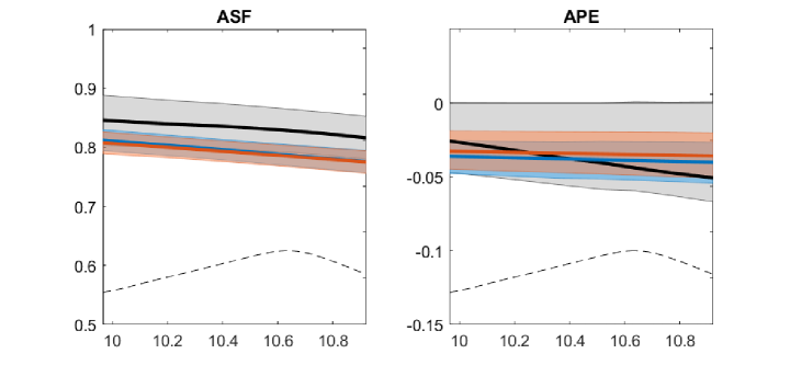
Figure 1: Estimated ASF and APE - Female Labor Force Participation

Notes: X-axes are potential values of log husband’s income. Black/blue/orange solid lines represent point estimates of the ASF and APE using the semiparametric/RE/CRE estimators. Bands with corresponding colors indicate the 90% bootstrap confidence intervals. Thin dashed lines at the bottom of both panels show the distribution of log husband’s income.

Figure 1 shows estimates of the ASF and APE across $\underline{x}_{t}$ together with the 90% bootstrap confidence intervals based on 500 bootstrap samples. For the ASF, all point estimates are downward sloping with respect to the husband’s income. The semiparametric estimator yields slightly higher participation probabilities compared to the RE and CRE.

For the APE, the semiparametric estimates are closer to zero for lower husband’s incomes and more negative for higher ones, while their RE and CRE counterparts are rather flat. Note that for continuous $\underline{x}_{t}^{(k)}$,

$$\text{APE}_{k,t}(\underline{x}_{t})=\beta_{0}^{(k)}\cdot f_{U_{t}-C}\left(\underline{x}_{t}^{\prime}\beta_{0}\right)=\beta_{0}^{(k)}\cdot\int_{\mathcal{C}}f_{U_{t}}(\underline{x}_{t}^{\prime}\beta_{0}+c)\,dF_{C}(c),$$

where $f_{U_{t}-C}$ denotes the pdf of $U_{t}-C$, i.e., a convolution of $-C$ and $U_{t}$. Thus, the slope of the APE with respect to $\underline{x}_{t}^{(k)}$ reflects the shapes of $f_{C}$ and $f_{U_{t}}$ as well as the magnitude of $\beta_{0}^{(k)}$. In this sense, the flatter APE profile with respect to the husband’s incomes in the RE and CRE could be due to the following three sources: (i) The RE and CRE feature a Gaussian $f_{C|V}$ and estimate the mean and variance of the Gaussian distribution. The estimated Gaussian variance could be fairly large to accommodate some non-Gaussian heterogeneity in $C|V$, and the resulting $\widehat{f}_{U_{t}-C}$ could be flatter (around the peak) than the true distribution. (ii) The RE and CRE assume a logistic $f_{U_{t}}$, which may deviate from the true data generating process. (iii) The smaller magnitudes of $\widehat{\beta}_{0}^{(k)}$ for RE and CRE could be due to misspecification of the distributions of $U_{t}$ and $C$ and, in turn, further lead to a milder slope of the APE profile. In contrast, the semiparametric estimator does not require the parametrization of $f_{C|V}$ or $f_{U_{t}}$, thus reducing potential biases due to misspecification.

Moreover, when using our flexible semiparametric estimator which does not constrain the distributions of $C$ or $U_{t}$, APEs with respect to the husband’s income are no longer significant. Highly significant APEs estimated via RE and CRE could partly be an artifact of their parametric restrictions. This is consistent with the empirical observation that married women’s labor supply choices became less sensitive to their husbands’ income around 1980 when baby boomers started constituting a larger portion of the labor force, and both partners contribute to housework and earnings more equally. Hence fewer married women were at the margin of labor force participation that could be nudged by temporary fluctuations in husbands’ income.

5 Conclusion

The distributions of the unobserved heterogeneity and the idiosyncratic errors play a crucial role in identifying partial effects in nonlinear panel models. In this paper, we first show the identification of the ASF, APE, and AME in a nonlinear semiparametric panel model with potentially unspecified distributions of the unobserved heterogeneity and of the idiosyncratic errors. To achieve point identification, we assume that units with the same value of the index $V$ have correspondingly similar distributions of their unobserved heterogeneity $C$. We also establish partial identification results when the support condition fails. We then develop three-step semiparametric estimators for the ASF and APE, and show their consistency and asymptotic normality in the Supplemental Appendix. Finally, we illustrate our semiparametric estimator in a study of determinants of women’s labor supply.

In Supplemental Appendix LABEL:sec:extensions we provided an identification result that applies to dynamic panel models. A generalization of our results to a broader class of dynamic models would be of interest for future work.

Appendix

This appendix is organized as follows. Appendix A provides additional identification results for $\beta_{0}$ under the index condition. Appendix B contains the proofs for the propositions and theorems in Sections 2 and Appendix A.

Appendix A Identification of $\beta_{0}$ under the Index Condition

The works cited in Section 2.2.2 do not use the index sufficiency in Assumption A3 to obtain the identification of $\beta_{0}$. However, it is possible to use A3 to show $\beta_{0}$’s identification under minimal additional assumptions on the model. Therefore, Assumption A2 may hold as a consequence of A3. In what follows, we first examine the baseline model with a known index function, and then explore the case where the index function is known up to finite-dimensional parameters.

A.1 Index = $v(\mathbf{X})$

Let us first consider the baseline scenario with a known index function $v(\mathbf{X})$.

Proposition A.1.

Let Assumptions A1 and A3 hold. Suppose there exists $s,t\in\{1,\ldots,T\}$ such that $s\neq t$, $\Psi_{s}(u,v)\equiv\mathbb{E}[Y_{s}|X_{s}^{\prime}\beta_{0}=u,V=v]$ is differentiable with $\frac{\partial}{\partial u}\Psi_{s}(u,v)\neq 0$, and that $W_{t}(\mathbf{x})\equiv\frac{\partial}{\partial x_{t}}v(\mathbf{x})^{\prime}$ has rank $d_{V}$. Normalize $\beta_{0}=(1,\tilde{\beta}_{0})$, where $\widetilde{\beta}_{0}\in\mathbb{R}^{d_{X}-1}$. Then, $\widetilde{\beta}_{0}$ is identified.

This result shows that $\beta_{0}$ can be identified (up to scale) with as few as two time periods, assuming that derivatives of $v(\mathbf{x})^{\prime}$ have rank $d_{V}$. This rank condition requires $d_{V}\leq d_{X}$, thus that the indices are of lower dimension than $\mathbf{X}$, the dimension of which is $d_{X}\times T$.

Note that we obtain $\beta_{0}$’s identification up to scale under the index sufficiency condition without assuming that $F_{U_{t}|C,\mathbf{X}}$ is stationary, or that $g_{t}(X_{t}^{\prime}\beta_{0},C,U_{t})$ has the functional form $\mathbbm{1}(X_{t}^{\prime}\beta_{0}+C+U_{t}\geq 0)$, or that $X_{t}^{\prime}\beta_{0}$ has large support. These three conditions are all required by Manski (1987) to obtain the identification of $\beta_{0}$. Therefore, one can relax a number of assumptions that lead to the identification of $\beta_{0}$ by using the index assumption $C\perp\!\!\!\perp\mathbf{X}|V$.

A.2 Index = $v(\mathbf{X})^{\prime}\gamma_{0}$

Now we investigate the scenario where the index $v(\mathbf{X})^{\prime}\gamma_{0}$ is known up to finite-dimensional parameters $\gamma_{0}$.

More specifically, suppose that there are $d_{V^{*}}$ indices, and each index is a linear combination of known functions of $\mathbf{X}$ with unknown coefficients. That is, $V^{*}=\left(v^{*}_{1}(\mathbf{X})^{\prime}\gamma^{*}_{1},\ldots,v^{*}_{d_{V^{*}}}(\mathbf{X})^{\prime}\gamma^{*}_{d_{V^{*}}}\right)\in\mathbb{R}^{1\times d_{V^{*}}}$. Note that $V^{*}$ can be multivariate with $d_{V^{*}}>1$. For notational simplicity, let $v(\mathbf{X})$ denote a collection of unique elements in $v^{*}_{1}(\mathbf{X}),\ldots,v^{*}_{d_{V^{*}}}(\mathbf{X})$ with dimension $d_{V}\times 1$, and $\gamma_{0}$ be the corresponding coefficient matrix with dimension $d_{V}\times d_{V^{*}}$ such that

$$V^{*}=\left(v^{*}_{1}(\mathbf{X})^{\prime}\gamma^{*}_{1},\ldots,v^{*}_{d_{V^{*}}}(\mathbf{X})^{\prime}\gamma^{*}_{d_{V^{*}}}\right)=v(\mathbf{X})^{\prime}\gamma_{0}.$$ (A.1)

The index structure in equation (A.1) determines the locations of zero entries in the coefficient matrix $\gamma_{0}$. Then, $\gamma^{*}_{1},\cdots,\gamma^{*}_{d_{V^{*}}}$ are the non-zero elements in each column of $\gamma_{0}$, while $v^{*}_{1}(\mathbf{X}),\ldots,v^{*}_{d_{V^{*}}}(\mathbf{X})$ correspond to the respective elements in $v(\mathbf{X}).$ Note that we only need to estimate these non-zero coefficients, which can be concatenated into a vector $\gamma^{*}=\left(\gamma^{*\prime}_{1},\cdots,\gamma^{*\prime}_{d_{V^{*}}}\right)^{\prime}\in\mathbb{R}^{d_{\gamma^{*}}}$.

Also note that the dimension of $V^{*}=V^{\prime}\gamma_{0}$ is usually lower than that of $V$. This dimension reduction facilitates the estimation of the conditional expectation of the outcomes given both $X_{t}^{\prime}\beta_{0}$ and the sufficient statistics, which is conducted via a nonparametric regression as detailed in Section 3 and Supplemental Appendix LABEL:sec:estimation2.

In this case, the index sufficiency condition can be stated as follows.

Assumption A12 (Unknown index sufficiency).

Given $V\equiv v(\mathbf{X})$, where $v:\mathbb{R}^{T\times d_{X}}\rightarrow\mathbb{R}^{d_{V}}$ is known, let $C\mid\mathbf{X}\overset{d}{=}C\mid V^{\prime}\gamma_{0}$ for a $\gamma_{0}\in\mathbb{R}^{d_{V}\times d_{V^{*}}}$.

Remark A.1.

For a given $V$, $C\perp\!\!\!\perp\mathbf{X}|V^{\prime}\gamma_{0}$ implies $C\perp\!\!\!\perp\mathbf{X}|V$, that is, A4 implies A3. See Appendix B for a formal proof. Intuitively, A4 introduces more structure on how $C$ depends on $\mathbf{X}$ through $V$, and thus helps reduce the dimensionality in estimation.

Under this Assumption A4 we can show that

$$\mathbb{E}[Y_{t}|\mathbf{X}=\underline{\mathbb{x}}] =\mathbb{E}[g_{t}(\underline{x}_{t}^{\prime}\beta_{0},C,U_{t})|V^{\prime}\gamma_{0}=v(\underline{\mathbb{x}})^{\prime}\gamma_{0}]$$

$$\equiv\Psi_{t}(\underline{x}_{t}^{\prime}\beta_{0},v(\underline{\mathbb{x}})^{\prime}\gamma_{0}),$$

an unknown function containing $d_{V^{*}}+1$ linear indices of $\underline{\mathbb{x}}$. Ichimura and Lee (1991) show that under conditions on the indices $(\underline{x}_{t}^{\prime}\beta_{0},v(\underline{\mathbb{x}})^{\prime}\gamma_{0})=(\underline{x}_{t}^{\prime}\beta_{0},v^{*}_{1}(\underline{\mathbb{x}})^{\prime}\gamma^{*}_{1},\ldots,v^{*}_{d_{V^{*}}}(\underline{\mathbb{x}})^{\prime}\gamma^{*}_{d_{V^{*}}})$, the parameters $\left(\beta_{0}^{\prime},\gamma^{*\prime}_{1},\cdots,\gamma^{*\prime}_{d_{V^{*}}}\right)^{\prime}$ are point identified up to scale and are estimable at a $\sqrt{N}$-rate. These conditions require that each index contains a continuous component, that none of the vectors $(X_{t},v^{*}_{1}(\mathbf{X}),\ldots,v^{*}_{d_{V^{*}}}(\mathbf{X}))$ are contained in one another, and the linear independence of the $1+d_{V^{*}}$ partial derivatives of $\Psi_{t}$ with respect to the indices. Considering the panel structure of the data, the indices $v(\mathbf{X})$ and $X_{t}$ generally contain different elements. This distinction arises because $v(\mathbf{X})$ can depend on $(X_{1},\ldots,X_{T})$, whereas $X_{t}$ is a single element of this vector. We now state a version of their Lemma 3 when regressors are continuous.

Proposition A.2 (Lemma 3 in Ichimura and Lee (1991)).

Assume that

1. Assumptions A1 and A4 hold;

2. Each of $(X_{t},v^{*}_{1}(\mathbf{X}),\ldots,v^{*}_{d_{V^{*}}}(\mathbf{X}))$ contains a continuous component with nonzero coefficient which is not contained in any of the other variables;

3. For some $t\in\{1,\ldots,T\}$, the function $\Psi_{t}(u,v)\equiv\mathbb{E}[Y_{t}|X_{t}^{\prime}\beta_{0}=u,V^{\prime}\gamma_{0}=v^{*}]$ is differentiable;

4. The partial derivatives $\left.\left(\frac{\partial\Psi_{t}(u,v)}{\partial u},\frac{\partial\Psi_{t}(u,v)}{\partial v^{*}_{1}},\cdots,\frac{\partial\Psi_{t}(u,v)}{\partial v^{*}_{d_{V^{*}}}}\right)\right|_{(u,v)=(X_{t}^{\prime}\beta_{0},v(\mathbf{X})^{\prime}\gamma_{0})}$ are not linearly dependent with probability 1.

Then, $\left(\beta_{0}^{\prime},\gamma^{*\prime}_{1},\cdots,\gamma^{*\prime}_{d_{V^{*}}}\right)^{\prime}$ are identified up to scale.

To summarize, we have highlighted a few identification approaches that result in the point identification (up to scale) of $\beta_{0}$. This list is not exhaustive, and it contains a new approach that uses the index sufficiency assumption.

Appendix B Proofs

B.1 Proofs for Section 2

Proof of Theorem 2.1.

We break this proof in three steps.

Step 1: We first show that $(C,U_{t})\perp\!\!\!\perp h(\mathbf{X})|V$ for any function $h$.

To see this, let $\mathcal{B}\subseteq\text{supp}(C,U_{t})$ and write

$$\mathbb{P}((C,U_{t})\in\mathcal{B}|h(\mathbf{X}),V) =\mathbb{E}[\mathbb{E}[\mathbbm{1}((C,U_{t})\in\mathcal{B})|C,h(\mathbf{X}),V]|h(\mathbf{X}),V]$$

$$=\mathbb{E}[\mathbb{E}[\mathbbm{1}((C,U_{t})\in\mathcal{B})|C,V]|h(\mathbf{X}),V]$$

$$=\mathbb{E}[\mathbb{E}[\mathbbm{1}((C,U_{t})\in\mathcal{B})|C,V]|V]$$

$$=\mathbb{P}((C,U_{t})\in\mathcal{B}|V).$$

The first and fourth equality follows from iterated expectations. The second equality follows from $U_{t}|(h(\mathbf{X}),V,C)\overset{d}{=}U_{t}|C\overset{d}{=}U_{t}|(V,C)$, which is implied by $U_{t}\perp\!\!\!\perp\mathbf{X}|C$ (Assumption A1.(ii)) and by $(h(\mathbf{X}),V)$ being functions of $\mathbf{X}$. To show the third equality holds, note that $C\perp\!\!\!\perp\mathbf{X}|V$ by A3. Since $h(\mathbf{X})$ is a function of $\mathbf{X}$, we also have that $C\perp\!\!\!\perp h(\mathbf{X})|V$. The set $\mathcal{B}$ was arbitrary thus $(C,U_{t})\perp\!\!\!\perp h(\mathbf{X})|V$.

Step 2: To show the ASF is identified, note that

$$\text{ASF}_{t}(\underline{x}_{t}) =\mathbb{E}[g_{t}(\underline{x}_{t}^{\prime}\beta_{0},C,U_{t})]$$

$$=\int_{\text{supp}(V)}\mathbb{E}[g_{t}(\underline{x}_{t}^{\prime}\beta_{0},C,U_{t})|V=v]\,dF_{V}(v)$$

$$=\int_{\text{supp}(V|X_{t}^{\prime}\beta_{0}=\underline{x}_{t}^{\prime}\beta_{0})}\mathbb{E}[g_{t}(\underline{x}_{t}^{\prime}\beta_{0},C,U_{t})|V=v]\,dF_{V}(v)$$

$$=\int_{\text{supp}(V|X_{t}^{\prime}\beta_{0}=\underline{x}_{t}^{\prime}\beta_{0})}\mathbb{E}[g_{t}(\underline{x}_{t}^{\prime}\beta_{0},C,U_{t})|X_{t}^{\prime}\beta_{0}=\underline{x}_{t}^{\prime}\beta_{0},V=v]\,dF_{V}(v)$$

$$=\int_{\text{supp}(V|X_{t}^{\prime}\beta_{0}=\underline{x}_{t}^{\prime}\beta_{0})}\mathbb{E}[Y_{t}|X_{t}^{\prime}\beta_{0}=\underline{x}_{t}^{\prime}\beta_{0},V=v]\,dF_{V}(v).$$

The second equality follows from iterated expectations, and the third from the support assumption in the theorem’s statement. The fourth follows from $(C,U_{t})\perp\!\!\!\perp X_{t}^{\prime}\beta_{0}|V$, which is shown in step 1 by setting $h(\mathbf{X})=X_{t}^{\prime}\beta_{0}$. The conditional expectations are well defined since $v\in\text{supp}(V|X_{t}^{\prime}\beta_{0}=\underline{x}_{t}^{\prime}\beta_{0})$ and $\underline{x}_{t}^{\prime}\beta_{0}\in\text{supp}(X_{t}^{\prime}\beta_{0})$.

The expression in the final equality depends on $\{\mathbb{E}[Y_{t}|X_{t}^{\prime}\beta_{0}=\underline{x}_{t}^{\prime}\beta_{0},V=v]:v\in\text{supp}(V|X_{t}^{\prime}\beta_{0}=\underline{x}_{t}^{\prime}\beta_{0})\}$, and $F_{V}$, the marginal distribution of $V$. By A2, $\beta_{0}$ is identified up to scale, thus the conditioning set $\{X_{t}^{\prime}\beta_{0}=\underline{x}_{t}^{\prime}\beta_{0}\}$ is identified since it is invariant to the scale of $\beta_{0}$. By definition, $\mathbb{E}[Y_{t}|X_{t}^{\prime}\beta_{0}=\underline{x}_{t}^{\prime}\beta_{0},V=v]$ is identified for $v\in\text{supp}(V|X_{t}^{\prime}\beta_{0}=\underline{x}_{t}^{\prime}\beta_{0})$. The marginal distribution of $V$ is also identified since $V=v(\mathbf{X})$ is a known function of observed $\mathbf{X}$. Hence, $\text{ASF}_{t}(\underline{x}_{t})$ is identified from the distribution of $(Y,\mathbf{X})$.

Step 3: For the APE, by the differentiability assumption we can write

$$\text{APE}_{k,t}(\underline{x}_{t}) =\frac{\partial}{\partial\underline{x}_{t}^{(k)}}\text{ASF}_{t}(\underline{x}_{t})=\lim_{\eta\to 0}\frac{\text{ASF}_{t}(\underline{x}_{t}+\eta e_{k})-\text{ASF}_{t}(\underline{x}_{t})}{\eta},$$ (B.1)

where $e_{k}$ is a vector of zeros with component $k$ equal to 1. Thus, $\text{APE}_{k,t}(\underline{x}_{t})$ is identified if $\text{ASF}_{t}(\underline{x}_{t}+\eta e_{k})$ is identified for all $\eta$ in a neighborhood of 0. By the above result, this is the case if $\text{supp}(V|X_{t}^{\prime}\beta_{0}=(\underline{x}_{t}+\eta e_{k})^{\prime}\beta_{0})=\text{supp}(V)$ for all $\eta$ in a neighborhood of 0. Note that $\text{supp}(V|X_{t}^{\prime}\beta_{0}=(\underline{x}_{t}+\eta e_{k})^{\prime}\beta_{0})=\text{supp}(V|X_{t}^{\prime}\beta_{0}=\underline{x}_{t}^{\prime}\beta_{0}+\eta\beta_{0}^{(k)})$, and that $\underline{x}_{t}^{\prime}\beta_{0}+\eta\beta_{0}^{(k)}$ lies in an arbitrary neighborhood of $\underline{x}_{t}^{\prime}\beta_{0}$ as $\eta\to 0$. Since we assumed that $\text{supp}(V|X_{t}^{\prime}\beta_{0}=u)=\text{supp}(V)$ for all $u$ in a neighborhood of $\underline{x}_{t}^{\prime}\beta_{0}$, $\text{ASF}_{t}(\underline{x}_{t}+\eta e_{k})$ is identified for $\eta$ sufficiently close to 0. Therefore $\text{APE}_{k,t}(\underline{x}_{t})$ is identified following the identification of the ASFs in equation (B.1). ∎

Proof of Theorem 2.2.

We can write the LAR as

$$\text{LAR}_{k,t}(\underline{\mathbb{x}}) =\left.\frac{\partial\mathbb{E}[g_{t}(\underline{x}_{t}^{\prime}\beta_{0},C,U_{t})|\mathbf{X}=\mathbf{x}]}{\partial\underline{x}_{t}^{(k)}}\right|_{\mathbf{x}=\underline{\mathbb{x}}}$$

$$=\left.\frac{\partial\mathbb{E}[g_{t}(\underline{x}_{t}^{\prime}\beta_{0},C,U_{t})|v(\mathbf{X})=v(\mathbf{x})]}{\partial\underline{x}_{t}^{(k)}}\right|_{\mathbf{x}=\underline{\mathbb{x}}}$$

$$=\lim_{\eta\to 0}\frac{\mathbb{E}[g_{t}(\underline{x}_{t}^{\prime}\beta_{0}+\eta\beta_{0}^{(k)},C,U_{t})|V=v(\underline{\mathbb{x}})]-E[g_{t}(\underline{x}_{t}^{\prime}\beta_{0},C,U_{t})|V=v(\underline{\mathbb{x}})]}{\eta}$$

$$=\lim_{\eta\to 0}\frac{1}{\eta}\left(\mathbb{E}[g_{t}(\underline{x}_{t}^{\prime}\beta_{0}+\eta\beta_{0}^{(k)},C,U_{t})|X_{t}^{\prime}\beta_{0}=\underline{x}_{t}^{\prime}\beta_{0}+\eta\beta_{0}^{(k)},V=v(\underline{\mathbb{x}})]\right.$$

$$\left.\qquad\qquad-\mathbb{E}[g_{t}(\underline{x}_{t}^{\prime}\beta_{0},C,U_{t})|X_{t}^{\prime}\beta_{0}=\underline{x}_{t}^{\prime}\beta_{0},V=v(\underline{\mathbb{x}})]\right)$$

$$=\lim_{\eta\to 0}\frac{\mathbb{E}[Y_{t}|X_{t}^{\prime}\beta_{0}=\underline{x}_{t}^{\prime}\beta_{0}+\eta\beta_{0}^{(k)},V=v(\underline{\mathbb{x}})]-\mathbb{E}[Y_{t}|X_{t}^{\prime}\beta_{0}=\underline{x}_{t}^{\prime}\beta_{0},V=v(\underline{\mathbb{x}})]}{\eta}$$

$$=\left.\frac{\partial\mathbb{E}[Y_{t}|X_{t}^{\prime}\beta_{0}=\underline{x}_{t}^{\prime}\beta_{0},V=v]}{\partial\underline{x}_{t}^{(k)}}\right|_{v=v(\underline{\mathbb{x}})}.$$

The first equality follows by the differentiability of $\mathbb{E}[Y_{t}(\underline{x}_{t})|\mathbf{X}=\mathbf{x}]$ in $\underline{x}_{t}^{(k)}$ and the definition of the LAR. The second follows $(C,U_{t})\perp\!\!\!\perp\mathbf{X}|v(\mathbf{X})$, which is shown in step 1 of the proof of Theorem 2.1. The third is by definition of partial derivatives, and the fourth follows from $v(\underline{\mathbb{x}})$ being in $\text{supp}(V|X_{t}^{\prime}\beta_{0}=\underline{x}_{t}^{\prime}\beta_{0}+\eta\beta_{0}^{(k)})$ for all sufficiently small $\eta$, which is assumed in the theorem statement. The fifth and sixth equalities follow immediately.

By A2, $\beta_{0}$ is identified up to scale, thus the conditioning set $\{X_{t}^{\prime}\beta_{0}=\underline{x}_{t}^{\prime}\beta_{0}\}$ is identified. Therefore, the conditional expectation $\mathbb{E}[Y_{t}|X_{t}^{\prime}\beta_{0}=\underline{x}_{t}^{\prime}\beta_{0}+\eta\beta_{0}^{(k)},V=v(\underline{\mathbb{x}})]$ is identified for sufficiently small $\eta$ if $v(\underline{\mathbb{x}})\in\text{supp}(V|X_{t}^{\prime}\beta_{0}=\underline{x}_{t}^{\prime}\beta_{0}+\eta\beta_{0}^{(k)})$, which is implied by $v(\underline{\mathbb{x}})\in\text{supp}(V|X_{t}^{\prime}\beta_{0}=u)$ for all $u$ in a neighborhood of $\underline{x}_{t}^{\prime}\beta_{0}$. This implies that $\text{LAR}_{k,t}(\underline{\mathbb{x}})$ is identified.

The proof of the identification of the AME follows from the identification of the LAR for all $\underline{\mathbb{x}}$ in $\text{supp}(\mathbf{X})$ (up to a $\mathbb{P}_{\mathbf{X}}$-measure zero set) and from

$$\text{AME}_{k,t} =\int_{\text{supp}(\mathbf{X})}\text{LAR}_{k,t}(\underline{\mathbb{x}})\,dF_{\mathbf{X}}(\underline{\mathbb{x}}).$$

∎

Proof of Theorem 2.3.

We first show that $\text{ASF}_{t}(\underline{x}_{t})\in\mathcal{A}_{t}(\underline{x}_{t})$ and then show the sharpness of this set.

Part 1: Bounds

By iterated expecations, we have that

$$\text{ASF}_{t}(\underline{x}_{t}) =\mathbb{E}[g_{t}(\underline{x}_{t}^{\prime}\beta_{0},C,U_{t})]$$

$$=\int_{\mathcal{V}}\mathbb{E}[g_{t}(\underline{x}_{t}^{\prime}\beta_{0},C,U_{t})|V=v]\,dF_{V}(v)$$

$$=\int_{\mathcal{V}_{t}(\underline{x}_{t}^{\prime}\beta_{0})}\mathbb{E}[g_{t}(\underline{x}_{t}^{\prime}\beta_{0},C,U_{t})|V=v]\,dF_{V}(v)+\int_{\mathcal{V}\setminus\mathcal{V}_{t}(\underline{x}_{t}^{\prime}\beta_{0})}\mathbb{E}[g_{t}(\underline{x}_{t}^{\prime}\beta_{0},C,U_{t})|V=v]\,dF_{V}(v).$$ (B.2)

The first term in (B.2) is

$$\int_{\mathcal{V}_{t}(\underline{x}_{t}^{\prime}\beta_{0})}\mathbb{E}[g_{t}(\underline{x}_{t}^{\prime}\beta_{0},C,U_{t})|V=v]\,dF_{V}(v) =\int_{\mathcal{V}_{t}(\underline{x}_{t}^{\prime}\beta_{0})}\mathbb{E}[g_{t}(\underline{x}_{t}^{\prime}\beta_{0},C,U_{t})|X_{t}^{\prime}\beta_{0}=\underline{x}_{t}^{\prime}\beta_{0},V=v]\,dF_{V}(v)$$

$$=\int_{\mathcal{V}_{t}(\underline{x}_{t}^{\prime}\beta_{0})}\mathbb{E}[Y_{t}|X_{t}^{\prime}\beta_{0}=\underline{x}_{t}^{\prime}\beta_{0},V=v]\,dF_{V}(v),$$

where the first equality is obtained by step 1 of the proof of Theorem 2.1 and by $v\in\mathcal{V}_{t}(\underline{x}_{t}^{\prime}\beta_{0})$.

The second term in (B.2) is bounded below by

$$\int_{\mathcal{V}\setminus\mathcal{V}_{t}(\underline{x}_{t}^{\prime}\beta_{0})}\mathbb{E}[g_{t}(\underline{x}_{t}^{\prime}\beta_{0},C,U_{t})|V=v]\,dF_{V}(v) \geq\int_{\mathcal{V}\setminus\mathcal{V}_{t}(\underline{x}_{t}^{\prime}\beta_{0})}\mathbb{E}[\underline{g}|V=v]\,dF_{V}(v)=\underline{g}\cdot\mathbb{P}(V\in\mathcal{V}\setminus\mathcal{V}_{t}(\underline{x}_{t}^{\prime}\beta_{0})).$$

By a similar argument, it is bounded above by $\overline{g}\cdot\mathbb{P}(V\in\mathcal{V}\setminus\mathcal{V}_{t}(\underline{x}_{t}^{\prime}\beta_{0}))$. We conclude that $\text{ASF}_{t}(\underline{x}_{t})\in\mathcal{A}_{t}(\underline{x}_{t})$.

Part 2: Sharpness

We consider the identified set for period $t=1$ without loss of generality. Let $a\in\mathcal{A}_{1}(\underline{x}_{1})$. We want to show that $a$ is in the identified set for $\text{ASF}_{1}(\underline{x}_{1})$. To achieve this, we are going to find structural functions $(\tilde{g}_{1},\ldots,\tilde{g}_{T})$ and a conditional distribution of $(\tilde{C},\tilde{U}_{1},\ldots,\tilde{U}_{T})|\mathbf{X}$ such that:

1. Assumptions A1 and A3 hold almost surely for $\left(\tilde{C},\{\tilde{U}_{t}\},\{\tilde{g}_{t}\}\right)$,

2. $\tilde{g}_{1}(\underline{x}_{1}^{\prime}\beta_{0},\tilde{C},\tilde{U}_{1})\in[\underline{g},\overline{g}]$ almost surely,

3. the distribution of $(\tilde{g}_{1}(X_{1}^{\prime}\beta_{0},\tilde{C},\tilde{U}_{1}),\ldots,\tilde{g}_{T}(X_{T}^{\prime}\beta_{0},\tilde{C},\tilde{U}_{T}))|\mathbf{X}$ equals the distribution of $Y|\mathbf{X}$,

4. $\mathbb{E}[\tilde{g}_{1}(\underline{x}_{1}^{\prime}\beta_{0},\tilde{C},\tilde{U}_{t})]=a$.

Below we first define $\left(\tilde{C},\{\tilde{U}_{t}\},\{\tilde{g}_{t}\}\right)$, and then we verify that they satisfy conditions (a)–(d).

First, we define $\tilde{U}_{t}$ based on the Skorokhod Representation Theorem. For $t=1,\ldots,T$ we can write

$$Y_{t} =Q_{Y_{t}|\mathbf{X}}(\tilde{U}_{t}|\mathbf{X})$$

where $Q_{Y_{t}|\mathbf{X}}$ is a conditional quantile function and $\tilde{U}_{t}|\mathbf{X}\sim\text{Unif}(0,1)$. We then let $\tilde{C}=V$ and

$$\tilde{g}_{1}(\underline{x}_{1}^{\prime}\beta_{0},\tilde{c},\tilde{u}_{1}) =Q_{Y_{1}|X_{1}^{\prime}\beta_{0},V}(\tilde{u}_{1}|\underline{x}_{1}^{\prime}\beta_{0},\tilde{c})\cdot\mathbbm{1}(\tilde{c}\in\mathcal{V}_{1}(\underline{x}_{1}^{\prime}\beta_{0}))+\tilde{a}\cdot\mathbbm{1}(\tilde{c}\in\mathcal{V}\setminus\mathcal{V}_{1}(\underline{x}_{1}^{\prime}\beta_{0}))$$

$$\tilde{g}_{2}(\underline{x}_{2}^{\prime}\beta_{0},\tilde{c},\tilde{u}_{2}) =Q_{Y_{2}|X_{2}^{\prime}\beta_{0},V}(\tilde{u}_{2}|\underline{x}_{2}^{\prime}\beta_{0},\tilde{c})\cdot\mathbbm{1}(\tilde{c}\in\mathcal{V}_{2}(\underline{x}_{2}^{\prime}\beta_{0}))+\underline{g}\cdot\mathbbm{1}(\tilde{c}\in\mathcal{V}\setminus\mathcal{V}_{2}(\underline{x}_{2}^{\prime}\beta_{0}))$$

$$\vdots$$

$$\tilde{g}_{T}(\underline{x}_{T}^{\prime}\beta_{0},\tilde{c},\tilde{u}_{T}) =Q_{Y_{T}|X_{T}^{\prime}\beta_{0},V}(\tilde{u}_{T}|\underline{x}_{T}^{\prime}\beta_{0},\tilde{c})\cdot\mathbbm{1}(\tilde{c}\in\mathcal{V}_{T}(\underline{x}_{T}^{\prime}\beta_{0}))+\underline{g}\cdot\mathbbm{1}(\tilde{c}\in\mathcal{V}\setminus\mathcal{V}_{T}(\underline{x}_{T}^{\prime}\beta_{0})),$$

where

$$\tilde{a} \equiv\frac{a-\int_{\mathcal{V}_{1}(\underline{x}_{1}^{\prime}\beta_{0})}\mathbb{E}[Y_{1}|X_{1}^{\prime}\beta_{0}=\underline{x}_{1}^{\prime}\beta_{0},V=v]\,dF_{V}(v)}{\mathbb{P}(V\in\mathcal{V}\setminus\mathcal{V}_{1}(\underline{x}_{1}^{\prime}\beta_{0}))}.$$ (B.3)

If $\mathbb{P}(V\in\mathcal{V}\setminus\mathcal{V}_{1}(\underline{x}_{1}^{\prime}\beta_{0}))=0$, $\text{ASF}_{1}(\underline{x}_{1})$ is point-identified by Theorem 2.1 and this proof is not needed. Thus, we assume $\mathbb{P}(V\in\mathcal{V}\setminus\mathcal{V}_{1}(\underline{x}_{1}^{\prime}\beta_{0}))>0$ for the remainder of this proof. Finally, the conditional quantiles above are well defined when $\tilde{c}\in\mathcal{V}_{t}(\underline{x}_{t}^{\prime}\beta_{0})$, so these expressions are well defined due to the indicator functions.

Then, we verify that the $\left(\tilde{C},\{\tilde{U}_{t}\},\{\tilde{g}_{t}\}\right)$ defined above satisfy conditions (a)–(d). First, we show that Assumptions A1 and A3 hold almost surely for $\left(\tilde{C},\{\tilde{U}_{t}\},\{\tilde{g}_{t}\}\right)$. We start by noting that $\mathbb{P}(V\in\mathcal{V}_{t}(X_{t}^{\prime}\beta_{0}))=\mathbb{E}[\mathbb{P}(V\in\mathcal{V}_{t}(X_{t}^{\prime}\beta_{0})|X_{t}^{\prime}\beta_{0})]=\mathbb{E}[1]=1$, therefore $\mathbbm{1}(V\in\mathcal{V}_{t}(X_{t}^{\prime}\beta_{0}))=1$ almost surely for $t=1,\ldots,T$. Also, since $Y_{t}=g_{t}(X_{t}^{\prime}\beta_{0},C,U_{t})$, we have that $Y_{t}\perp\!\!\!\perp\mathbf{X}|(X_{t}^{\prime}\beta_{0},V)$ by Assumptions A1.(ii) and A3 for the original $\left(C,\{U_{t}\},\{g_{t}\}\right)$. Therefore, $Q_{Y_{t}|\mathbf{X}}(\cdot|\mathbf{X})=Q_{Y_{t}|X_{t}^{\prime}\beta_{0},V}(\cdot|X_{t}^{\prime}\beta_{0},V)$. From these, we obtain that

$$Y_{1} =Q_{Y_{1}|\mathbf{X}}(\tilde{U}_{1}|\mathbf{X})$$

$$\overset{a.s.}{=}Q_{Y_{1}|X_{1}^{\prime}\beta_{0},V}(\tilde{U}_{1}|X_{1}^{\prime}\beta_{0},V)\cdot\mathbbm{1}(V\in\mathcal{V}_{1}(X_{1}^{\prime}\beta_{0}))+\tilde{a}\cdot\mathbbm{1}(V\in\mathcal{V}\setminus\mathcal{V}_{1}(X_{1}^{\prime}\beta_{0}))$$

$$=\tilde{g}_{1}(X_{1}^{\prime}\beta_{0},\tilde{C},\tilde{U}_{1})$$

where we used that $\mathbbm{1}(V\in\mathcal{V}_{1}(X_{1}^{\prime}\beta_{0}))=1$ a.s., and $\tilde{C}=V$. Likewise, for $t=2,\ldots,T$ we have that

$$Y_{t} =Q_{Y_{t}|\mathbf{X}}(\tilde{U}_{t}|\mathbf{X})$$

$$\overset{a.s.}{=}Q_{Y_{t}|X_{t}^{\prime}\beta_{0},V}(\tilde{U}_{t}|X_{t}^{\prime}\beta_{0},V)\cdot\mathbbm{1}(V\in\mathcal{V}_{t}(X_{t}^{\prime}\beta_{0}))+\underline{g}\cdot\mathbbm{1}(V\in\mathcal{V}\setminus\mathcal{V}_{t}(X_{t}^{\prime}\beta_{0}))$$

$$=\tilde{g}_{t}(X_{t}^{\prime}\beta_{0},\tilde{C},\tilde{U}_{t}).$$

Therefore, Assumption A1.(i) holds almost surely for $\left(\tilde{C},\{\tilde{U}_{t}\},\{\tilde{g}_{t}\}\right)$. Assumption A1.(ii) holds for $\left(\tilde{C},\{\tilde{U}_{t}\},\{\tilde{g}_{t}\}\right)$, since $\tilde{U}_{t}\perp\!\!\!\perp\mathbf{X}$ by construction and $\tilde{C}=V=v(\mathbf{X})$, a function of $\mathbf{X}$. Assumption A1.(iii) holds for $\left(\tilde{C},\{\tilde{U}_{t}\},\{\tilde{g}_{t}\}\right)$ because $[\underline{g},\overline{g}]$ is a bounded interval. Assumption A3 holds trivially for $\left(\tilde{C},\{\tilde{U}_{t}\},\{\tilde{g}_{t}\}\right)$ since $\tilde{C}\perp\!\!\!\perp\mathbf{X}|V$ when $\tilde{C}=V$, as is the case here. Therefore all model assumptions hold almost surely for $\left(\tilde{C},\{\tilde{U}_{t}\},\{\tilde{g}_{t}\}\right)$.

Second, note that $\tilde{a}\in[\underline{g},\overline{g}]$ by $a\in\mathcal{A}_{1}(\underline{x}_{1})$, so $\tilde{g}_{1}(\underline{x}_{1},\tilde{C},\tilde{U}_{1})\in[\underline{g},\overline{g}]$ almost surely.

Third, the distributions of $(\tilde{g}_{1}(X_{t}^{\prime}\beta_{0},\tilde{C},\tilde{U}_{1}),\ldots,\tilde{g}_{T}(X_{T}^{\prime}\beta_{0},\tilde{C},\tilde{U}_{T}))|\mathbf{X}$ and $Y|\mathbf{X}$ coincide because $(\tilde{g}_{1}(X_{1}^{\prime}\beta_{0},\tilde{C},\tilde{U}_{1}),\ldots,\tilde{g}_{T}(X_{T}^{\prime}\beta_{0},\tilde{C},\tilde{U}_{T}))=Y$ almost surely, as shown above.

Finally, we verify that the implied ASF, $\mathbb{E}[\tilde{g}_{1}(\underline{x}_{1}^{\prime}\beta_{0},\tilde{C},\tilde{U}_{1})]$, equals $a$:

$$\mathbb{E}[\tilde{g}_{1}(\underline{x}_{1}^{\prime}\beta_{0},\tilde{C},\tilde{U}_{1})]$$

$$=\int_{\mathcal{V}}\mathbb{E}[\tilde{g}_{1}(\underline{x}_{1}^{\prime}\beta_{0},\tilde{C},\tilde{U}_{1})|V=v]\,dF_{V}(v)$$

$$=\int_{\mathcal{V}_{1}(\underline{x}_{1}^{\prime}\beta_{0})}\mathbb{E}[Q_{Y_{1}|X_{1}^{\prime}\beta_{0},V}(\tilde{U}_{1}|\underline{x}_{1}^{\prime}\beta_{0},V)|V=v]\,dF_{V}(v)+\int_{\mathcal{V}\setminus\mathcal{V}_{1}(\underline{x}_{1}^{\prime}\beta_{0})}\mathbb{E}[\tilde{a}|V=v]\,dF_{V}(v)$$

$$=\int_{\mathcal{V}_{1}(\underline{x}_{1}^{\prime}\beta_{0})}\mathbb{E}[Q_{Y_{1}|X_{1}^{\prime}\beta_{0},V}(\tilde{U}_{1}|X_{1}^{\prime}\beta_{0},V)|X_{1}^{\prime}\beta_{0}=\underline{x}_{1}^{\prime}\beta_{0},V=v]\,dF_{V}(v)+\tilde{a}\cdot\mathbb{P}(V\in\mathcal{V}\setminus\mathcal{V}_{1}(\underline{x}_{1}^{\prime}\beta_{0})).$$ (B.4)

The first equality follows by iterated expectations, the second by substituting the expression for $\tilde{g}_{1}$, and the third from $\tilde{U}_{1}\perp\!\!\!\perp X_{1}^{\prime}\beta_{0}|V$, which is implied by $\tilde{U}_{1}\perp\!\!\!\perp\mathbf{X}$. By $\tilde{U}_{1}\perp\!\!\!\perp(X_{1}^{\prime}\beta_{0},V)$ and by properties of conditional quantiles, we have that

$$\mathbb{E}[Q_{Y_{1}|X_{1}^{\prime}\beta_{0},V}(\tilde{U}_{1}|X_{1}^{\prime}\beta_{0},V)|X_{1}^{\prime}\beta_{0}=\underline{x}_{1}^{\prime}\beta_{0},V=v] =\int_{0}^{1}Q_{Y_{1}|X_{1}^{\prime}\beta_{0},V}(\tilde{u}_{1}|\underline{x}_{1}^{\prime}\beta_{0},v)\,d\tilde{u}_{1}$$

$$=\mathbb{E}[Y_{1}|X_{1}^{\prime}\beta_{0}=\underline{x}_{1}^{\prime}\beta_{0},V=v].$$ (B.5)

Substituting the expression for $\tilde{a}$ in (B.3) and the expression for the conditional mean in (B.5) into equation (B.4), we obtain

$$\mathbb{E}[\tilde{g}_{1}(\underline{x}_{1}^{\prime}\beta_{0},\tilde{C},\tilde{U}_{1})] =\int_{\mathcal{V}_{1}(\underline{x}_{1}^{\prime}\beta_{0})}\mathbb{E}[Y_{1}|X_{1}^{\prime}\beta_{0}=\underline{x}_{1}^{\prime}\beta_{0},V=v]\,dF_{V}(v)$$

$$\qquad+\frac{a-\int_{\mathcal{V}_{1}(\underline{x}_{1}^{\prime}\beta_{0})}\mathbb{E}[Y_{1}|X_{1}^{\prime}\beta_{0}=\underline{x}_{1}^{\prime}\beta_{0},V=v]\,dF_{V}(v)}{\mathbb{P}(V\in\mathcal{V}\setminus\mathcal{V}_{1}(\underline{x}_{1}^{\prime}\beta_{0}))}\cdot\mathbb{P}(V\in\mathcal{V}\setminus\mathcal{V}_{1}(\underline{x}_{1}^{\prime}\beta_{0}))$$

$$=a,$$

which concludes the proof. ∎

Proof of Corollary 2.1.

Note that $\mathbb{E}[Y_{t}|X_{t}^{\prime}\beta_{0}=\underline{x}_{t}^{\prime}\beta_{0},\mathbf{X}=\mathbf{x}]=\mathbb{E}[Y_{t}|\mathbf{X}=\mathbf{x}]$ for all $\mathbf{x}\in\text{supp}(\mathbf{X}|X_{t}^{\prime}\beta_{0}=\underline{x}_{t}^{\prime}\beta_{0})$. Also note that $\mathbb{P}(\mathbf{X}\in\text{supp}(\mathbf{X})\setminus\text{supp}(\mathbf{X}|X_{t}^{\prime}\beta_{0}=\underline{x}_{t}^{\prime}\beta_{0}))=\mathbb{P}(X_{t}^{\prime}\beta_{0}\neq\underline{x}_{t}^{\prime}\beta_{0})$. We also have that $C\perp\!\!\!\perp\mathbf{X}|\mathbf{X}$ trivially. This corollary follows from a combination of the above results with an application of Theorem 2.3 for $V=\mathbf{X}$. ∎

B.2 Proofs for Appendix Section A

Proof of Proposition A.1.

Without loss of generality, let $s=1$ and $t=2$. We start by computing

$$\frac{\partial}{\partial x_{1}}\mathbb{E}[Y_{1}|\mathbf{X}=\mathbf{x}] =\frac{\partial}{\partial x_{1}}\Psi_{1}(x_{1}^{\prime}\beta_{0},v(\mathbf{x}))=\left.\frac{\partial}{\partial u}\Psi_{1}(u,v(\mathbf{x}))\right|_{u=x_{1}^{\prime}\beta_{0}}\begin{pmatrix}1\\ \widetilde{\beta}_{0}\end{pmatrix}+W_{1}(\mathbf{x})\frac{\partial}{\partial v}\Psi_{1}(x_{1}^{\prime}\beta_{0},v)|_{v=v(\mathbf{x})}$$

$$\frac{\partial}{\partial x_{2}}\mathbb{E}[Y_{1}|\mathbf{X}=\mathbf{x}] =\frac{\partial}{\partial x_{2}}\Psi_{1}(x_{1}^{\prime}\beta_{0},v(\mathbf{x}))=W_{2}(\mathbf{x})\frac{\partial}{\partial v}\Psi_{1}(x_{1}^{\prime}\beta_{0},v)|_{v=v(\mathbf{x})}.$$

where

$$W_{t}(\mathbf{x}) =\frac{\partial}{\partial x_{t}}v(\mathbf{x})^{\prime}\in\mathbb{R}^{d_{X}\times d_{V}}.$$

From the second equation above, we can recover

$$\frac{\partial}{\partial v}\Psi_{1}(x_{1}^{\prime}\beta_{0},v)|_{v=v(\mathbf{x})}=\left(W_{2}(\mathbf{x})^{\prime}W_{2}(\mathbf{x})\right)^{-1}W_{2}(\mathbf{x})^{\prime}\frac{\partial}{\partial x_{2}}\mathbb{E}[Y_{1}|\mathbf{X}=\mathbf{x}]$$

since $W_{2}(\mathbf{x})$ has rank $d_{V}$.

Therefore, we can identify

$$\left.\frac{\partial}{\partial u}\Psi_{1}(u,v(\mathbf{x}))\right|_{u=x_{1}^{\prime}\beta_{0}}\begin{pmatrix}1\\ \widetilde{\beta}_{0}\end{pmatrix}=\frac{\partial}{\partial x_{1}}\mathbb{E}[Y_{1}|\mathbf{X}=\mathbf{x}]-W_{1}(\mathbf{x})\left(W_{2}(\mathbf{x})^{\prime}W_{2}(\mathbf{x})\right)^{-1}W_{2}(\mathbf{x})^{\prime}\frac{\partial}{\partial x_{2}}\mathbb{E}[Y_{1}|\mathbf{X}=\mathbf{x}].$$ (B.6)

By the assumption that $\frac{\partial\Psi_{1}(u,v(\mathbf{x}))}{\partial u}\neq 0$, $\widetilde{\beta}_{0}$ is point identified as the ratio of the elements in equation (B.6). ∎

Proof of Proposition A.2.

By Assumption A1, we have that

$$\mathbb{E}[Y_{t}|\mathbf{X}] =\int_{\text{supp}(C,U_{t}|\mathbf{X})}g_{t}(X_{t}^{\prime}\beta_{0},c,u_{t})\,dF_{C,U_{t}|\mathbf{X}}(c,u_{t}|\mathbf{X})$$

$$=\int_{\text{supp}(C,U_{t}|\mathbf{X})}g_{t}(X_{t}^{\prime}\beta_{0},c,u_{t})\,dF_{C,U_{t}|V^{\prime}\gamma_{0}}(c,u_{t}|v(\mathbf{X})^{\prime}\gamma_{0})$$

$$=\Psi_{t}(X_{t}^{\prime}\beta_{0},v(\mathbf{X})^{\prime}\gamma_{0})$$

where the second equality follows from $(C,U_{t})\perp\!\!\!\perp\mathbf{X}|v(\mathbf{X})^{\prime}\gamma_{0}$, which follows from Assumption A4 and step 1 in the proof of Theorem 2.1. The result then follows immediately from Lemma 3 in Ichimura and Lee (1991) with no additive index in the outcome equation and when applied to continuous regressors only. ∎

Proof of Remark A.1.

First note that $C\perp\!\!\!\perp\mathbf{X}|V^{\prime}\gamma_{0}$ implies that $C\perp\!\!\!\perp h(\mathbf{X})|V^{\prime}\gamma_{0}$ for any function $h$. We then have that

$$C|V \overset{d}{=}C|V,V^{\prime}\gamma_{0}\overset{d}{=}C|V^{\prime}\gamma_{0}.$$

The first distributional equality is from $V^{\prime}\gamma_{0}$ being known when $V$ is known, and the second follows from $C\perp\!\!\!\perp h(\mathbf{X})|V^{\prime}\gamma_{0}$ selecting $h(\mathbf{X})=v(\mathbf{X})$. Also, $C\perp\!\!\!\perp\mathbf{X}|V^{\prime}\gamma_{0}$ implies $C|\mathbf{X}\overset{d}{=}C|V^{\prime}\gamma_{0}$. Combining these equations, we have that $C|\mathbf{X}\overset{d}{=}C|V$. ∎

References

- (1)
- Abrevaya (1999) Abrevaya, J. (1999): “Leapfrog estimation of a fixed-effects model with unknown transformation of the dependent variable,” Journal of Econometrics, 93(2), 203–228.
- Abrevaya (2000) (2000): “Rank estimation of a generalized fixed-effects regression model,” Journal of Econometrics, 95(1), 1–23.
- Abrevaya and Hsu (2021) Abrevaya, J., and Y.-C. Hsu (2021): “Partial effects in non-linear panel data models with correlated random effects,” The Econometrics Journal, 24(3), 519–535.