Optimizations for Hardware-in-the-Loop-Based V2X Validation Platforms

Abstract

Connectivity and automation are increasingly getting importance in the automotive industry, which is observing a radical change from vehicles driven by humans to fully automated and remotely controlled ones. The test and validation of all the related devices and applications is thus becoming a crucial aspect; this is raising the interest on hardware-in-the-loop (HiL) platforms which reduce the need for complicated field trials, thus limiting the costs and delay added to the process. With reference to the test and validation of vehicle-to-everything (V2X) communications aspects, and assuming either sidelink LTE/5G-V2X or IEEE 802.11p/bd technologies, in this work we focus on the real-time HiL simulation of the information exchanged by one vehicle under test and the surrounding, simulated, objects. Such exchange must be reproduced in a time-efficient manner, with elaborations done fast enough to allow testing the applications in real-time. More precisely, we discuss the simulation of non-ideal positioning and channel propagation taking into account current impairments. We also provide details on optimization solutions that allowed us to trade-off minor loss in accuracy with a significant reduction of the computation time burden, reaching up to more than one order of magnitude speed increase in our experiments.

I Introduction

By the rapid growth of urbanization worldwide, connected and autonomous vehicles will increasingly play an important role to improve safety in our cities. The promises are to reduce the number of accidents and fatalities, to improve traffic and energy efficiency [1], to enable commercial applications such as toll collection, and so on [2]. Many applications are indeed being designed and developed for the intelligent transport system (ITS), which are based on V2X communications [3, 4, 5]. These applications take advantage of information about the status and movements of nearby vehicles and objects to take prompt and smart decisions. To this aim, several messages have been defined both in Europe and in the US, including basic safety messages, cooperative awareness messages, decentralized environmental notification messages, or are under definition, such as collective perception messages or vulnerable road user awareness messages. The main wireless technologies that are currently used or expected to be used in short range to exchange these messages are IEEE 802.11p (corresponding to ITS-G5 in Europe) and cellular- (C-V2X). Safety is one of the most important aspects of such systems, and conducting extensive tests for the validation and reliability of the applications before moving to production is crucial. Noticeably, performing real-world field tests is very challenging for many reasons; first, providing a controlled environment to perform tests in the desired scenarios imposes relevant extra costs. Second, even assuming large budgets, it is technically not feasible to involve large number of nodes or to address a large number of scenarios. Finally, performing tests on the road implies a significant overhead in terms of manpower and dedicated time. . These types of challenges rise the importance of using simulations and emulations platforms as the initial stage of the validation process. In particular, simulators are often used as first step which come, however, with some level of abstractions such as modeling of radio propagation, global navigation satellite system (GNSS) accuracy, traffic flow, etc. Besides the fact that not all of the aspects are implemented with the same level of details, simulators can hardly address all the issues that are related to the use of the real hardware and software.

For these reasons, the use of the so-called hardware-in-the-loop (HiL) platforms is raising increasing importance in the validation process of modern cars [6]. Differently from standard simulators, in the design and development of a HiL platform the ability to guarantee real-time processing is a critical aspect. Focusing on wireless communications, in most works the challenges of real-world tests are addressed with simulators/emulators (e.g., [7, 8]) but the solutions do not appear to be able to work at real-time because of the high latency that is introduced. In other cases (e.g., in [9]), the focus is indeed on real-time simulations but the radio-link communication conditions, which introduce significant delay to the simulators, is not discussed. Moreover, although there are other HiL platforms implemented and introduced in the literature, they mostly rely on the traffic simulators to receive the status of the objects; it means that they lack the real effects that may happen due to the GPS inaccuracy or real communication link condition between the objects. For example, in [10, 11, 12] the HiL platforms are implemented for different use cases of CAVs. In [10], only vehicle-to-infrastructure (V2I) communications are considered and in [11], big attention is paid to the driver assistance system and communication is performed V2V only, whereas in [12], an accurate tracking of target vehicle speed and engine operating points is provided. However, none of these works target a mechanism that can guarantee the validity of the received packets by considering the various channel conditions or GNSS errors in real time.

The reason why the channel quality is normally not considered is that it adds processing delay hardly compatible with the real time nature of an HiL platform. A solution might be to use probabilistic models, such as proposed [13], which however cannot reproduce a specific environment. Even in [14], where channel quality is indeed considered based on the nodes distance, the links are either assumed all in line-of-sight (LOS) or in non-line-of-sight (NLOS). As explained, all the approaches currently proposed in literature have some limitations if used in the validation process of real hardware and software for CAVs and this motivated us to identify the new solutions proposed in this work.

The platform under design focuses on a specific vehicle with connectivity and advanced driver assistance systems (ADAS), hereafter called ego-vehicle (EGO), and this paper especially focuses on the software component within the HiL platform which aims at defining the propagation and positioning aspects affecting the perception of the surrounding at the EGO. The contribution of the paper can be summarized as follows:

first, we describe the architecture aspects of our validation platform which are relevant for connectivity; second, we introduce a method for reproducing GNSS positioning inaccuracy in a controlled environment; then, we discuss the optimization of path-loss evaluations in order to fulfil the stringent timing requirements in large scenarios. Finally, we elaborate on the accuracy of the proposed approach by showing results in a case-study scenario.

Figure 1: System Architecture

II System Architecture

HiL validation platforms are typically constituted by hardware parts such as connected road side units and on-board units, and software parts such as channel simulators or road traffic simulators; in our case, they are jointly cooperating with ADAS components to evaluate and validate the performance of CAV implementations. The system architecture of the platform under development related to connectivity is represented in Fig. 1. It is composed of three main components (from right to left in the figure): (i) the simulation of the environment and vehicle movements, performed by the scenario/traffic simulator (TRS); (ii) the generation, through the external management unit (EMU), of messages produced by the vehicles and other nodes around the device under test, i.e., the EGO; and (iii) the EGO itself, where the applications to be validated are implemented.

On the one hand, the TRS is dedicated to the simulation of the road layout, the mobility of all the vehicles and possible pedestrians or bikes, and the buildings. In the results shown later, as TRS we have adopted the open-source simulation of urban mobility (SUMO) [15] that provides outputs to both the EMU (building and device positions) and the EGO (EGO position). On the other hand, the EMU receives the position of the buildings and other static objects at the beginning of the simulation, and an updated position of the moving nodes during the simulation from the TRS. Accordingly, it evaluates the quality of the links and determines which and when messages are to be transmitted from the surrounding nodes to the EGO. The process goes through the identification of propagation conditions (further elaborated in Section IV), the calculation of the received power, the evaluation of lost messages, the addition of realistic GNSS inaccuracies (further elaborated in Section III), and the transmission through a real ITS-station (ITS-S), which can be either an OBU or an RSU. Finally, the EGO receives its own simulated positions from the TRS (possibly alters them to account the realistic GNSS inaccuracies) and the information from the neighboring devices from the EMU, through the hardware OBU. All the information is processed by the applications installed on the EGO and the correct operation is evaluated.

At the time of writing this paper, virtual OBUs and RSUs are being used, emulating both IEEE 802.11p and side-link LTE-V2X communications [16]. It is remarkable that the focus of this paper is the optimization of parts that will remain via software, as detailed in the following sections, in order to allow real-time processing, and thus the use of virtual devices do not alter the validity of the detailed solutions. Moreover, in the initial implementation of the platform, the focus is on scenarios with a limited number of vehicles around the EGO and thus a low level of channel usage. For this reason, the impact of collisions is initially neglected and will be added as a second step.

III Simulating localization inaccuracies

One aspect that needs careful consideration in the validation process of V2X applications is the impact of localization. In fact, most of the applications rely on information about the position of the EGO and other objects. In the real implementation, the latitude, longitude, and height of the EGO are derived from the on-board GNSS receiver, while the position of the other devices is embedded in the messages received from the other nodes, which are on their own generated on the basis of information obtained from GNSS receivers. In the platform, the exact position is provided by the TRS.

The positioning systems do provide the location with some degree of inaccuracy. To take into account the position inaccuracies in our platform, a random variable error is introduced to the exact position of the vehicles provided by TRS, both inside the EGO and the EMU.

The literature about localization accuracy is quite fragmented and, at the best of the authors’ knowledge, a complete and unified model to represent the error accuracy is not available [17], [18]. Hence, to evaluate the reliability of the GNSS, we performed experiments on the road with a global positioning system (GPS) device. In particular, we positioned the car in a fixed location in the city of Bologna (Italy), collected the information received by the ITS-S, and elaborated the outline. As an example of the performed elaboration, Fig. 2 shows the positioning error in time compared to the long-term average assumed as the ground-truth. As visible, the error varies significantly during the time, with peaks of more than 5 m. It is also observable that the error is highly correlated, which is an expected effect of the relative movement between the satellites and the Earth. In addition, we also performed experiments traveling several times along a given route in order to verify the validity of our conclusions also while moving on the road.

From the described measurements, we derived a positioning error with an absolute value following a Gaussian distribution with zero mean and a given standard deviation and an angle distributed uniformly between $0$ and $2\pi$. The distance root mean square error obtained in our measurements was equal to 2.32 m.

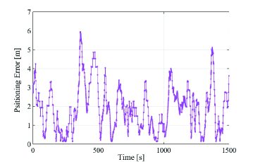
Figure 2: Positioning error vs. time variation.

In order to reproduce a correlated error, the model proposed for the shadowing in [19] was used as a reference. In particular, the correlated magnitude, denoted as $\mu$, and angle, denoted as $\theta$, are derived from the following equations

$$\mu=\ e^{-T/t_{corr}}\times\mu_{-1}+\sqrt{1-e^{-2T/t_{corr}}\ }\times N_{\mu}$$

$$\theta=\ e^{-T/t_{corr}}\times\theta_{-1}+\sqrt{1-e^{-2T/t_{corr}}\ }\times N_{\theta}$$ (1)

where $T$ is the time elapsed from the last time instant (the last instant when the error was calculated), $\mu_{-1}$ and $\theta_{-1}$ are the amplitude and phase calculated in the last time instant, respectively, and $N_{\mu}$ and $N_{\theta}$ are the new uncorrelated samples of the magnitude and angle. The parameter $t_{corr}$ is used to control the degree of correlation. A smaller $t_{corr}$ causes a quick variation of the error, whereas a larger $t_{corr}$ implies a slow variation of the error. Through our experiments, we derived a $t_{corr}=10$ s. The location known at the EGO and included in the messages sent by the EMU is thus obtained in terms of latitude, denoted as $v_{\text{lat}}$, and longitude, denoted as $v_{\text{lon}}$, by applying the following equations

$$v_{\text{lat}}=v_{\text{lat}}^{*}+\big{(}\mu\times\sin{(\theta)}\big{)}$$

$$v_{\text{lon}}=v_{\text{lon}}^{*}+\big{(}\mu\times\cos{(\theta)}\big{)}$$ (2)

where $v_{\text{lat}}^{*}$ and $v_{\text{lon}}^{*}$ are the exact latitude and longitude provided by the TRS, respectively.

Fig. 3 represents the output of a simulation using the inaccurate GNSS positioning model. Specifically, the blue line represents the exact location while the red line provides the estimated location including the positioning error.

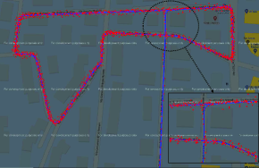
Figure 3: GNSS accuracy error.

IV Assessing the propagation conditions

Another aspect that deserved particular attention in our implementation is the derivation of propagation conditions, which means in particular identifying whether the communication link between the two ITS-Ss is in LOS or not, before computing the path-loss accordingly. There are in fact various models proposed in the literature for the calculation of the path-loss in vehicular scenarios, the last one being the one in ETSI TR 103 257-1 [20], summarized in Annex A, and all of them provide different calculations given the LOS or NLOS conditions, hereafter named propagation conditions. Whereas calculating the path loss as a function of the distance is immediate once the propagation conditions are known, identifying if the link between two nodes is obstructed or not might imply more complex calculations. Considering that such an evaluation is required continuously during the simulation due to the mobility of nodes, a huge time and processing effort might be required, possibly compromising the real-time nature of the simulations.

In this section, we describe the process adopted in our platform to identify the propagation conditions per each link between the EGO and the other vehicles moving in the scenario. The process is summarized through pseudo code in Algorithm 1.

Input: Vehicle and building positions;

Output: Propagation conditions;

1 % Init building positions

2 $buildings$ $\leftarrow$ building positions;

3 for each time step do

4       % Update vehicle positions

5       $e$ $\leftarrow$ ego-vehicle position;

6       $vehicles$ $\leftarrow$ other vehicle positions;

7      

8      % Reset conditions

9       $conditions$($\forall v\in vehicles$) = LOS;

10      % Select vehicles within $InRangeV$

11       for $v\in vehicles$ do

12             if $dist(e,v)<R_{v}$ then

13                  $InRangeV\leftarrow v$;

14            

15      

16      % Select buildings within $InRangeB$

17       for $b\in buildings$ do

18             if $dist(e,b)<R_{b}$ then

19                  $InRangeB\leftarrow b$;

20            

21      

22      % Cycle over the other vehicles

23       for $rv\in InRangeV$ do

24             % Init flag

25             $flag$ = false;

26             % Check NLOS due to buildings

27             for $rb\in InRangeB$ do

28                   if $InBtw(rb,rv,e)$ then

29                        $flag$ = true

30                         break

31                  

32            

33            if $flag$ then

34                   $conditions$(rv) = NLOSb;

35                   break

36            

37            % Check NLOS due to vehicles

38             for $sv\in InRangeV\setminus rv$ do

39                   if $InBtw(sv,rv,e)$ then

40                        $flag$=true

41                         break

42                  

43            if $flag$ then

44                  $conditions$(rv) = NLOSv;

45                   break

46            % else LOS conditions: nothing to do

47            

48      

49

Algorithm 1 Propagation conditions assessment.

At the beginning of the simulation, the TRS informs the EMU about the building positions and the static objects (e.g., traffic light or static road works) and provides updated positions of all moving nodes every time interval, hereafter denoted as step. Within each step, the simulator should be able to evaluate the quality of all links in order to maintain the real-time nature of the simulation. Hence, during each step, the link between the EGO and each of the other vehicles is categorized as either LOS, non-line-of-sight due to buildings (NLOSb), or non-line-of-sight due to vehicles (NLOSv). A building obstructs the link if any of the walls intersects the segment connecting the EGO to a target vehicle. Moreover, a third vehicle obstructs the link if its distance, $d_{\text{orth}}$, from the segment connecting the EGO and the target vehicle is below a given threshold, with $d_{\text{orth}}$ calculated as

$$d_{\text{orth}}=\frac{\left|mx_{\text{sv}}-y_{\text{sv}}-mx_{\text{e}}+y_{\text{e}}\right|}{\sqrt{m^{2}+1}}\;,$$ (3)

where $m=\frac{y_{\text{rv}}-y_{\text{e}}}{x_{\text{rv}}-x_{\text{e}}}$, $x_{\text{e}}$ and $y_{\text{e}}$ being the EGO coordinates, $x_{\text{rv}}$, $y_{\text{rv}}$ the other (target) vehicle coordinates, and $x_{\text{sv}}$, $y_{\text{sv}}$ those of the third considered vehicle.

In principle, if $N_{\text{v}}$ is the number of vehicles in the scenario and $N_{\text{b}}$ the number of buildings, this operation requires in each simulation step to evaluate $(N_{\text{v}}-1)\times N_{\text{b}}$ times if a given building obstructs a link and $(N_{\text{v}}-1)\times(N_{\text{v}}-2)$ if a third vehicle obstructs a link, which appears hardly feasible within a single step.

The first and rather obvious observation, in order to reduce the computation effort, is that as soon as NLOSb conditions are observed due to one building, there is no need to proceed with the others or with the third vehicles. Similarly, when no building obstructs the link and one of the third vehicles is found to be between the communicating nodes, NLOSv conditions are met and there is no reason to proceed with the other third vehicles. To further reduce the burden of the calculation, two scanning ranges are applied to the EGO, $R_{\text{b}}$ and $R_{\text{v}}$, which limit the considered buildings and other vehicles, respectively, to a maximum distance from the EGO. The rational for $R_{\text{b}}$ is that those buildings which are far from the EGO are expected not to relevantly impact on the assessment of NLOSb conditions and it is thus assumed that they can be neglected during the simulation. This assumption is verified through a case study in Section V. The setting of $R_{\text{v}}$ should instead consider the relevance of the information received by the EGO; the information received by far vehicles might be not relevant, for example for an intersection collision warning application. In general, $R_{\text{v}}$ will be not larger than the maximum range for the given settings and $R_{\text{b}}$ will not be larger than $R_{\text{v}}$. The buildings and vehicles obtained through this process are hereafter called relevant objects.

In summary, in each simulation step the process detailed in Algorithm 1 is performed: i) the list of relevant target vehicles $N_{\text{v}}^{\text{(r)}}$ (those within $R_{\text{v}}$) and the list of relevant buildings (those within $R_{\text{b}}$) are evaluated; ii) a cycle over the $N_{\text{v}}^{\text{(r)}}-1$ vehicles around the EGO is performed and per each of them, first the NLOSb conditions (considering the relevant buildings only) and, in case the NLOSv conditions (considering only the relevant vehicles) are verified.

Once the propagation conditions are evaluated, the calculation of the path-loss, the addition of correlated shadowing, and the definition of lost messages are done with marginal addition of computation effort. At the output of this process, the messages that are evaluated to be correctly received by the EGO (CAMs in our case study) are obtained; they are then passed to the function in charge to introduce the positioning inaccuracy (described in Section III) and then transmitted through the real ITS-S.

V Performance evaluation

To verify the performance of the solutions described in the previous sections, and especially by the proposed propagation conditions evaluation, we considered a portion of the city of Bologna with a maximum point-to-point distance of 3.2 km as shown in Fig. 4. Vehicles, simulated with SUMO, periodically transmit CAMs using IEEE 802.11p, which exploits a 10 MHz channel in the 5.9 GHz frequency band; transmission power $P_{\text{t}}=23$ dBm and sensitivity $P_{\text{r}}=-82$ dBm are assumed. The urban channel model described in ETSI TR 103 257-1 [20], reported in Annex A, is adopted with log-normal correlated shadowing characterized by 3 dB standard deviation and 10 m decorrelation distance (as suggested in 3GPP TR 36.885 [19]). A laptop equipped with a core-i7 processor with 2.59 GHz CPU frequency was used to run the simulation.

Figure 4: Map of the simulated area.

Fig. 5 illustrates the average number of vehicles at each simulation step in the three different channel conditions (LOS, NLOSb, and NLOSv) as well as the total traffic when the scanning ranges ($R_{\text{b}}$ and $R_{\text{v}}$) are set to the 3.2 km, which is the maximum distance of the map and thus is equivalent to infinity. The reduction of the scanning ranges, $R_{\text{b}}$ and $R_{\text{v}}$, allows to consider a smaller area of the map, thus decreasing the simulation time.

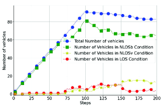
Figure 5: Distribution of traffic.

In Fig. 6, the performance of the proposed approximation is measured, with a fixed $R_{\text{v}}=3.2$ km (i.e., all vehicles in the scenario are considered). In particular, the accuracy of the proposed approximation is evaluated in Fig. 6(a) in terms of number of vehicles in NLOSb conditions varying the building scanning range $R_{b}$. The results reveal that by reducing $R_{b}$ from 3.2 km to 500 m, the number of nodes in NLOSb which are not identified as such is around 3% of the whole nodes; whereas further decreasing this range to 300 m, the same number becomes around 7%. Moreover, for any value of $R_{b}$ greater than 900 m, the loss of system accuracy (in terms of missing nodes in NLOSb condition) is almost negligible (less than 1% on average). It should also be remarked that, with $R_{b}\geq 900$ m, the few nodes not detected in NLOSb conditions are all farther than 2 km from the EGO and thus not really relevant for the performance of the tested applications.

(a) Number of vehicles found in NLOSb condition.

(b) Simulation delay.

Figure 6: Simulation performance; varying $R_{\text{b}}$, with $R_{\text{v}}=3.2$ km.

On the other hand, Fig. 6(b) illustrates the simulation delay versus simulation steps for the same buildings scanning ranges $R_{b}$, keeping $R_{\text{v}}=3.2$ km. The simulation delay is the processing delay introduced by the EMU from the instant when it receives the information from the TRS to the instant when it forwards the results to the hardware and should be as low as possible to allow the real-time integration of HiL. As observable, when $R_{b}$ decreases to 500 m and 300 m, the maximum delay decreases from around 2.2 s to 350 ms and less than 200 ms, respectively.

The simulation delay is then plotted in Fig. 7 by fixing the $R_{\text{b}}=900$ m and varying the $R_{\text{v}}$. The $R_{\text{v}}$ can be reduced depending on the application’s obligation. For example, for some safety applications such as intersection collision warning (ICW) that do not need to cover the nodes in a wide area, reducing the $R_{v}$ to 300 m, the maximum simulation delay would be around 50 ms. In this case, it is not significant to evaluate the accuracy as the range of 900 m for $R_{\text{b}}$ almost guarantees it.

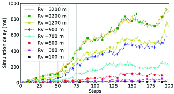
Figure 7: Simulation delay; varying $R_{\text{v}}$, with $R_{\text{b}}=900$ m.

The impact of the approach is finally evaluated in Fig. 8 in terms of averaged delay, over the 50 simulation steps with highest traffic, varying both $R_{\text{v}}$ and $R_{\text{b}}$. Specifically, Fig. 8 shows that the simulation delay can be reduced down to 18 ms for $R_{\text{v}}=R_{\text{b}}=100$ m and that remains lower than 1 s (i.e., the larger time interval between CAM generations [21]) for several combinations of the two scanning ranges.

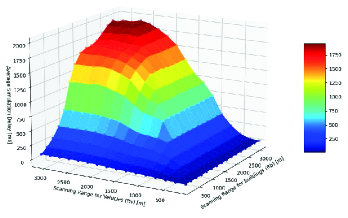
Figure 8: Average simulation delay as a function of the two scanning ranges $R_{\text{v}}$ and $R_{\text{b}}$.

VI Conclusion and future directions

In this paper, we addressed the topic of real-time HiL simulation platforms to validate V2X applications in a controlled lab environment. After illustrating the architecture of the validation platform under development, solutions to consider localization accuracy and impact of wireless channel impairments were detailed. The performance of the proposed solutions were derived with reference to a case-study in an urban environment and illustrated that our simulation platform is able to work at run-time with reasonable delay, compatible with most of the safety applications defined in ETSI TS 102 637-2. Currently, small channel load is considered and the access protocols are assumed ideal, with no losses due to collisions; as a next step, models taking into account the current conditions (vehicle density, access technology with modulation and coding scheme, message size, etc.) will be derived to overcome this limitation and still allow real-time processing required when hardware is in the loop. The detailed software will be part of a HiL platform integrating ADAS and connectivity for the validation of CAVs.

Appendix A: path loss model

The ETSI TR 103 257-1 [20] is used here as path-loss model while other channel models can be found in [22, 23, 24]. The considered model distinguishes between highway and urban scenarios, as well as LOS, NLOSb, and NLOSv conditions.

In particular, the following equations model the path loss for the urban environment in LOS and NLOSb

$${P_{\text{l}}}_{\mathrm{LOS}}=38.77+16.7\log_{10}(d_{\text{3D}})+18.2\log_{10}(f_{\text{c}})$$ (4)

$${P_{\text{l}}}_{\mathrm{NLOSb}}=36.85+30\log_{10}(d_{\text{3D}})+18.9\log_{10}(f_{\text{c}})$$ (5)

where $d_{\text{3D}}$ is the euclidean transmitter-receiver distance and $f_{\text{c}}$ is the central frequency in GHz (set to 5.9).

The attenuation for the NLOSv conditions is calculated as

$${P_{\text{l}}}_{\mathrm{NLOSv}}={{P^{\prime}}_{\text{l}}}_{\mathrm{NLOSv}}+{P_{\text{l}}}_{\mathrm{LOS}}$$ (6)

$${{P^{\prime}}_{\text{l}}}_{\mathrm{NLOSv}}=\begin{cases}6.9+20\log_{10}\sqrt{(\nu-0.1)^{2}+1}+\\ +\nu-0.1\leavevmode\nobreak\ \leavevmode\nobreak\ \leavevmode\nobreak\ \leavevmode\nobreak\ \leavevmode\nobreak\ \leavevmode\nobreak\ \leavevmode\nobreak\ \leavevmode\nobreak\ \leavevmode\nobreak\ \leavevmode\nobreak\ \leavevmode\nobreak\ \leavevmode\nobreak\ \leavevmode\nobreak\ \leavevmode\nobreak\ \leavevmode\nobreak\ \leavevmode\nobreak\ \leavevmode\nobreak\ \leavevmode\nobreak\ \leavevmode\nobreak\ \leavevmode\nobreak\ \leavevmode\nobreak\ \text{for}\leavevmode\nobreak\ \nu>0.7\\ 0\leavevmode\nobreak\ \leavevmode\nobreak\ \leavevmode\nobreak\ \leavevmode\nobreak\ \leavevmode\nobreak\ \leavevmode\nobreak\ \leavevmode\nobreak\ \leavevmode\nobreak\ \leavevmode\nobreak\ \leavevmode\nobreak\ \leavevmode\nobreak\ \leavevmode\nobreak\ \leavevmode\nobreak\ \leavevmode\nobreak\ \leavevmode\nobreak\ \leavevmode\nobreak\ \leavevmode\nobreak\ \leavevmode\nobreak\ \leavevmode\nobreak\ \leavevmode\nobreak\ \leavevmode\nobreak\ \leavevmode\nobreak\ \leavevmode\nobreak\ \leavevmode\nobreak\ \leavevmode\nobreak\ \leavevmode\nobreak\ \leavevmode\nobreak\ \leavevmode\nobreak\ \leavevmode\nobreak\ \leavevmode\nobreak\ \text{otherwise.}\end{cases}\;,$$

$\nu=\sqrt{2}\ \frac{H}{r_{\text{f}}}$, $H$ is the difference in height between the obstacle and the straight link from transmitter to receiver, $r_{\text{f}}$ is the first Fresnel zone radius that can be approximated as $r_{\text{f}}=\sqrt{\frac{\lambda d_{\text{1}}d_{\text{2}}}{d_{\text{1}}+d_{\text{2}}}}$, $d_{\text{1}}$ and $d_{\text{2}}$ are the distances from the blocking vehicle to the transmitter and receiver, respectively, and $\lambda$ is the wavelength.

References

- [1] M. Wegener, T. Plum, M. Eisenbarth, and J. Andert, “Energy Saving Potentials of Modern Powertrains Utilizing Predictive Driving Algorithms in Different Traffic Scenarios,” Part D: Journal of Automobile Engineering, vol. 234, no. 4, pp. 992–1005, 2020.
- [2] H. Zhou, W. Xu, J. Chen, and W. Wang, “Evolutionary V2X Technologies Toward the Internet of Vehicles: Challenges and Opportunities,” Proceedings of the IEEE, vol. 108, no. 2, pp. 308–323, 2020.
- [3] M. Menarini, P. Marrancone, G. Cecchini, A. Bazzi, B. M. Masini, and A. Zanella, “TRUDI: Testing Environment for Vehicular Applications Running with Devices in the Loop,” in proc. of ICCVE. IEEE, 2019.
- [4] L. Chen and C. Englund, “Cooperative Intersection Management: A Survey,” IEEE Transactions on Intelligent Transportation Systems, vol. 17, no. 2, pp. 570–586, 2015.
- [5] M. Di Vaio, P. Falcone, R. Hult, A. Petrillo, A. Salvi, and S. Santini, “Design and Experimental Validation of a Distributed Interaction Protocol for Connected Autonomous Vehicles at a Road Intersection,” IEEE Transactions on Vehicular Technology, vol. 68, no. 10, 2019.
- [6] M. Eisenbarth, M. Wegener, R. Scheer, J. Andert, D. S. Buse, F. Klingler, C. Sommer, F. Dressler, P. Reinold, and R. Gries, “Toward Smart Vehicle-to-Everything Connected Powertrains: Driving Real Component Test Benches in a Fully Interactive Virtual Smart City,” IEEE Vehicular Technology Magazine, 2020.
- [7] S. D. Gupta, C.-C. Lin, and C.-Y. Chan, “BSM Emulator-Advanced Vehicle Safety Application Testbed,” in proc. of ITSC. IEEE, 2012.
- [8] Y. P. Fallah and S. O. Gani, “Efficient and High Fidelity DSRC Simulation,” in Connected Vehicles. Springer, 2019, pp. 217–243.
- [9] G. Shah, R. Valiente, N. Gupta, S. O. Gani, B. Toghi, Y. P. Fallah, and S. D. Gupta, “Real-time Hardware-in-the-Loop Emulation Framework for DSRC-Based Connected Vehicle Applications,” in proc. of CAVS. IEEE, 2019.
- [10] J. Ma, F. Zhou, Z. Huang, C. L. Melson, R. James, and X. Zhang, “Hardware-in-the-Loop Testing of Connected and Automated Vehicle Applications: A Use Case for Queue-Aware Signalized Intersection Approach and Departure,” Transportation Research Record, vol. 2672, no. 22, pp. 36–46, 2018.
- [11] J. Ma, F. Zhou, Z. Huang, and R. James, “Hardware-in-the-Loop Testing of Connected and Automated Vehicle Applications: A Use Case for Cooperative Adaptive Cruise Control,” in proc. of ITSC. IEEE, 2018.
- [12] M. A. M. Zulkefli, P. Mukherjee, Z. Sun, J. Zheng, H. X. Liu, and P. Huang, “Hardware-in-the-Loop Testbed For Evaluating Connected Vehicle Applications,” Transportation Research Part C: Emerging Technologies, vol. 78, pp. 50–62, 2017.
- [13] M. Boban, X. Gong, and W. Xu, “Modeling the Evolution of Line-Of-Sight Blockage for V2V Channels,” in proc. of VTC. IEEE, 2016.
- [14] A. Bazzi, T. Blazek, M. Menarini, B. M. Masini, A. Zanella, C. Mecklenbräuker, and G. Ghiaasi, “A Hardware-in-the-Loop Evaluation of the Impact of the V2X Channel on the Traffic-Safety Versus Efficiency Trade-offs,” in Proc. of EuCAP, 2020.
- [15] P. A. Lopez, M. Behrisch, L. Bieker-Walz, J. Erdmann, Y.-P. Flötteröd, R. Hilbrich, L. Lücken, J. Rummel, P. Wagner, and E. Wießner, “Microscopic Traffic Simulation Using SUMO,” in proc. of ITSC. IEEE, 2018.
- [16] A. Bazzi, C. Campolo, A. Molinaro, A. O. Berthet, B. M. Masini, and A. Zanella, “On Wireless Blind Spots in the C-V2X Sidelink,” IEEE Transactions on Vehicular Technology, vol. 69, no. 8, 2020.
- [17] A. Bais and Y. Morgan, “Analysis of Positioning Uncertainty in Vehicular Environment,” in proc. of FIT. IEEE, 2016.
- [18] G. S. Bierman, “Error Modeling for Differential GPS.” AIR FORCE INST OF TECH WRIGHT-PATTERSON AFB OH, Tech. Rep., 1995.
- [19] “3GPP; Technical Specification Group Radio Access Network; Study on LTE-based V2X Services;(Release 14),” Sophia Antipolis Valbonne, FRANCE, 3GPP TR 36.885 V14.0.0, Tech. Rep., June, 2016.
- [20] “Intelligent Transport Systems (ITS); Access Layer; Part 1: Channel Models for the 5,9 GHz Frequency Band,” Sophia Antipolis Cedex, FRANCE, ETSI TR 103 257-1 V1.1.1, Tech. Rep., May, 2019.
- [21] “ITS; Vehicular Communications; Basic Set of Applications; Part 2: Specification of Cooperative Awareness Basic Service,” Sophia Antipolis Cedex, FRANCE, ETSI TS 102 637-2 V1.2.1, Tech. Rep., March, 2011.
- [22] J. Meinilä, P. Kyösti, T. Jämsä, and L. Hentilä, “WINNER II Channel Models,” Radio Technologies and Concepts for IMT-Advanced, 2009.
- [23] C. Schneider, M. Narandzic, M. Kaske, G. Sommerkorn, and R. S. Thoma, “Large Scale Parameter for the WINNER II Channel Model at 2.53 GHz in Urban Macro Cell,” in proc. of VTC. IEEE, 2010.
- [24] J. Meinila, P. Kyosti, L. Hentila, T. Jamsa, E. Suikkanen, E. Kunnari, and M. Narandzic, “D5. 3: WINNER+ Final Channel Models,” Wireless World Initiative New Radio WINNER, pp. 119–172, 2010.