Anomaly Detection in Predictive Maintenance: A New Evaluation Framework for Temporal Unsupervised Anomaly Detection Algorithms

Abstract

The research in anomaly detection lacks a unified definition of what represents an anomalous instance. Discrepancies in the nature itself of an anomaly lead to multiple paradigms of algorithms design and experimentation. Predictive maintenance is a special case, where the anomaly represents a failure that must be prevented. Related time series research as outlier and novelty detection or time series classification does not apply to the concept of an anomaly in this field, because they are not single points which have not been seen previously and may not be precisely annotated. Moreover, due to the lack of annotated anomalous data, many benchmarks are adapted from supervised scenarios.

To address these issues, we generalise the concept of positive and negative instances to intervals to be able to evaluate unsupervised anomaly detection algorithms. We also preserve the imbalance scheme for evaluation through the proposal of the Preceding Window ROC, a generalisation for the calculation of ROC curves for time series scenarios. We also adapt the mechanism from a established time series anomaly detection benchmark to the proposed generalisations to reward early detection. Therefore, the proposal represents a flexible evaluation framework for the different scenarios. To show the usefulness of this definition, we include a case study of Big Data algorithms with a real-world time series problem provided by the company ArcelorMittal, and compare the proposal with an evaluation method.

1 Introduction

The label of anomaly detection is assigned to a variety of problems with different natures and use cases [1]. For instance, time series anomalies in predictive maintenance or fault detection [2], process data in security [3] or graph data in social media [4]. Other names like outliers, exceptions, rare events or novelties are used with different intention or in different study fields. The disparity of scenarios itself develops into multiple evaluation schemas, that may cause confusion and proposals that are not correctly evaluated.

The variety of nomenclature to the scenarios has been addressed by other researchers [5]. Their proposed taxonomy uses rare event for supervised temporal data with a class imbalance and the task of classifying these time series into known classes [6]. The broadly used term of anomaly is reserved for the supervised classification task of non-temporal data with highly imbalanced class distribution [7]. In the semi-supervised scenarios [8], where only normal data is available during training time, some authors use the term of One-Class classification [1], [9], while others prefer Novelty detection, remarking the interest in the unseen instances [10]. Another broadly used term is outlier detection [8], usually associated with unsupervised classification and frequently in relation with the term noise, more related to the data instances that divert from normal observations but not enough to be considered to have been produced by another mechanism, which is in the ultimate instance the aim of abnormal data detection algorithms.

In the specific scenario of predictive maintenance, as a special case of anomaly detection in time series and the situation considered in this work, the events of interest are represented by singular points that require an intervention. A similar circumstance happens with time series anomaly detection algorithms: they evaluate singular points to predict an event that does not affect only an instant but a subsequent interval.

As expected, all the mentioned different scenarios use specific measures and experimentation setups to validate their results. On the one hand, most of these measures come from supervised imbalanced scenarios, as the recall of the minority or new classes, or some combination of the precision and recall, like the F-measure, or measures derived from the ROC (Receiver Operating Characteristic) Curve, such as the Area under the curve (AUC) [11]. On the other hand, for those scenarios where the main focus is the temporal component, the proposals include a measure for the earliness of the detection [12] with the aim of minimising the probability of a failure.

In summary, there are many different scenarios for abnormal behaviour that go by the name of anomaly detection and many associated measures which have associated drawbacks with respect to the addressed task of predictive maintenance:

• The benefits of the imbalance problem approach are diluted by the omission of the temporal component.

• The evaluation of the earliness in the detection is aggregated for a more understandable comprehension through more parameters, making more difficult the task of adaptation to general and real case scenarios.

To overcome these issues, we gather the different approaches to anomalous event detection, unifying the evaluation schemes and the implications of the instance and class assignation into an new evaluation framework for temporal unsupervised anomaly detection algorithms for scenarios where the events of interest have a uncertain relation with the data. The proposed evaluation framework definition starts with a temporal window that precedes the anomaly. The general consideration is that a positive instance is detected when the algorithm triggers an alarm within the window. However, this raises some logic issues: What is the upper window limit? What is the usefulness of windows so wide that they gather all the instances? Theoretically, we can consider the whole interval as the previous window. Then, we would have only a positive instance relative to the last logged event, and negative instances posterior to this last instance, which lack a relevant meaning for a study, as random detectors would benefit from these schemes. Nonetheless, the upper limit is subject to the researcher interests. The proposed framework could be outlined using the following components:

• In the first place, we define a transformation of the instances, from time-stamps to intervals, with an aggregation that provides a wider view of the event of an anomaly through the inclusion of a parameter for the length of the window that precedes each annotated event.

• Then, we describe what are the options for the aggregation and what are the implications, including an earliness-aware aggregation derived from the Numenta Anomaly Benchmark (NAB).

• The next component is the Preceding Window ROC (pw-ROC), that generalise the definition of the classic ROC curve to include the previously mentioned window length parameter. The aggregation of these pw-ROC shapes the ROC surface, as the parameter of the length of the preceding window represents the third dimension.

Therefore, the complete process generates a figure that provides the information about the quality of the algorithm, not only at all the possible levels of threshold to assign the anomaly labels but also to different levels of distance until the event of interest. Two versions of this proposal has been implemented: one classical version using python, and another version using pySpark to be capable of handling Big Data time series problems. This proposal has two implementations in python, one classic implementation and a distributed version using pySpark to be capable of handling Big Data time series problems and is available as a repository in GitHub.

To validate the usefulness of the proposal, we include the evaluation using this framework of three state-of-the-art algorithms and examine their results using a real data set provided by ArcelorMittal. We also evaluate the algorithms using a scoring system for anomalous range and compare this evaluation with our method to analyse the benefits of the proposal. The popularity of the scenario, where the use of unsupervised algorithms is desired due to the lack of certainty about the possible events that arise, although the events of interest can be annotated through observation for algorithms evaluation, shows the reliability of the proposed benchmark for such task.

In summary, the major contributions of this work are:

• Description of the distinctive features of the anomaly detection problem for time series scenarios of predictive maintenance.

• Proposal of evaluation method for the described scenarios with associated software for Big Data time series.

• Case study with a comparison between the outcome of the evaluation method proposal and an evaluation proposal for a similar scenario.

This paper is organised as follows: Section 2 presents the current state of anomaly detection evaluation systems, approaches and quality measures. In Section 3, the proposed evaluation framework is presented and justified theoretically. Section 4 includes the experiments and comparison performed to validate the applicability and validity of the proposal. Finally, Section 5 concludes the paper.

2 Background in anomaly detection evaluation

In this section, we describe four different approaches for the evaluation of anomaly detection algorithms, particularly for those situations where temporal component should be taken into account. The most used strategy is to consider the problem of anomaly detection (without a temporal component) as an imbalanced classification task. In predictive maintenance the events of interest can be transformed not into positive instance in a classification problem but into the target variable for a regression algorithms perspective. More recent works shift back to classification tasks with extra measures to reward the desired earliness in the detection. For all these methodologies, the underlying anomaly detection aim is to discern the timestamp when an anomaly occurs using the observations $x_{i},i=1,\dots,N$, i. e. to provide an accurate label $y_{i}$ for each instance that reflects the time series behaviour.

2.1 Anomaly detection evaluation for non-temporal data

For methods that provide a ranking of the instances according to their outlierness, the precision at $n$ ($P@n$) is defined as the proportion of the first ranked $n$ instances that are anomalies [13]. If $n$ is equal to the number of outliers in the dataset, the the author denominates $P@n$ as the $R$-precision. This makes the reliability of this measure compromised by the $n$ parameter, especially in unsupervised scenarios [14]. The $P@n$ measure would ignore the temporal component in predictive maintenance scenarios, considering the observations as isolated instances.

The problem of the balance is addressed in imbalance classification with the ROC curve [15]. ROC space is defined as an $[0,1]\times[0,1]$ space using True Positive Rate (TPR or sensibility, represented in $Y$ axis) and False Positive Rate (FPR or $1-$ specificity, represented in $X$ axis) [16]. For example, an algorithm with a perfect TPR and FPR would be in $(0,1)$. The extension of this concept is used generally for algorithms that provide scores or probabilities in imbalanced classification scenarios. Then, we can get different ROC points for each possible threshold and TPR (and FPR) increases as this threshold does.

2.2 Regression transformation

As described in Section 1, temporal data represents a great proportion of real-world problems. The most common task in time series problems is to model the desired time series, a scenario where the temporal component is intrinsic to the studied data, so the evaluation measure does not need to be aware of this temporal nature and they use a regression measure like the Root Mean Squared Error (RMSE) or the Error Ratio [17, 18]. However, for the specific case of anomaly detection in time series, the interest relies on the anomalous events that take place at a certain point in the time series, not the values of the time series themselves.

One approach for the evaluation of anomaly detection in time series comes from the transformation of the problem of rare event detection into a regression problem, where for each timestamp $i=1,\dots,N$, the target is the remaining time $r_{i}$ until the failure or the stop [19]. This is an interesting proposal, as in predictive maintenance we aim to maximise productivity with minimal repairs costs through the knowledge of our system. Then, reliable predictions of the available time until the failure ($R(x_{i})=\hat{r}_{i},i=1,\dots,N$) may help us in this task. The evaluation measure is the RMSE, as in many regression problems. This approach broaches the relevance of time in failure detection, and using the RMSE as the quality measure overcomes the detachment between the singular predictions and the continuous nature of the problem.

2.3 Rare event detection and earliness

In the time series classification problem scenario, the earliness is defined as the mean percentage of the length $t_{j}$ of each time series $X_{j}$ needed to provide a class label $Y_{j}$. The pertinence of taking into account the distance until the predicted event is also addressed by Zhang et al.  [20]. In this work, they transform the rare event detection problem into a classification one through the definition of a horizon window, in which the instances must be classified as anomalous. A weight is assigned to these positive instances to give more relevance to these closer to an event.

2.4 Range-Based Anomaly Detection Measures

A relevant scenario for temporal anomaly detection is the consideration of time intervals as anomalies [21, 22]. In these works, Tatbul et al. propose a range-based generalisation for the concepts of precision, recall and the $F_{1}$ measure. The expected output of the algorithm is a label for each instance, that is transformed to intervals of contiguous anomalous instance. These measures evaluate each anomalous interval ($R_{i}$ for real anomalous intervals and $P_{i}$ for predicted anomalous intervals) using the score based on the detection ($E(R_{i},P)$, the existence of at least a timestamp that belongs to $R_{i}$ and any $P_{i}\in P$), and the overlap ($O(R_{i},P)$, the proportion of detected timestamps in $R_{i}$). Therefore, the subject of interest of this method are anomalous intervals, labeled as such. Their proposal allows the modification of certain parameters to reward different behaviours, such as an early or late detection of the anomaly within the real anomalous interval.

This measure has a straightforward modification to evaluate algorithms for the studied scenario, defining the anomalous time intervals as the windows preceding the event of interest. Then, to validate our proposal we compare it with this evaluation method.

2.5 Numenta Anomaly Detection Benchmark

A vital problem for time series anomaly researches is that there are no extended benchmarks for the comparison of the performance of streaming anomaly detection algorithms. A fundamental proposal is the Numenta Anomaly Benchmark [12]. This benchmark proposes a scoring function and provides a set of manually labelled real-world time series. Here, four weights $A_{TP},A_{FP},A_{TN},A_{FN}$ are defined for true positives, false positives, etc. The absolute value of these weights are between 0 and 1, being $A_{TN}$ and $A_{TP}$ positives and $A_{FN},A_{FP}$ negatives, to penalise the errors. The default scenario described in the Numenta Anomaly Benchmark defines the weights $A_{TP}=A_{TN}=1$, and $A_{FP}=A_{FN}=-1$, although different values could be settled for different profiles. Then, a window is defined previous to each anomaly. In these windows, only the first alarm provided by the algorithm is kept, while the windows that precedes an anomaly that do not have an alarm are considered to be false negative instances, that could be denoted as missed windows. Let $y$ be the relative position of the alarm within the interval. Then, the score is defined as:

$$\sigma^{A}(y)=(A_{TP}-A_{FP})\left(\frac{1}{1+e^{5y}}\right)-1.$$ (1)

Therefore, the detections at the end of the interval ($y=0$) are evaluated as 0, and a detection just after the interval receives a smaller penalisation. Then, the raw score for each data set is defined as the sum of the scores of the detections in the positive windows ($Y_{d}$) plus the product of $A_{FN}$ and the number of missed windows, $f_{d}$:

$$\mathrm{Score}:\sum_{y\in Y_{d}}\sigma^{A}(y)+A_{FN}f_{d}.$$ (2)

This benchmark is subject to some criticisms made by Singh and Olinsky [23]. Some of these criticisms refer to the impracticality of the system in a real-world streaming scenario as the allegedly good performance of the studied algorithms is not enough for practical applications. Moreover, there are some issues concerning the scoring function, as it is not clearly defined for every situation. In their analysis, it is shown that their score over-reward avoiding false positives and allows a low recall of the anomalies. We address these issues concerning the scoring system through the combination of an imbalanced scenario metric as the AUC with the window partition of the temporal space and the weighting system for rewarding early detection.

2.6 Summary of quality measures

A summary of the different scenarios and used quality measures is included in Table 1.

Task	Description	Evaluation	Formula
time series class.	Classification of complete time series.	Accuracy	$\frac{\sum_{X\in\mathbf{X}_{test}}\mathbb{I}[c(X)=Y]}{|\mathbf{X}_{test}|}$
	Percentage of the length of the time series needed for the classification.	Earliness	$\frac{\sum_{x\in\mathbf{X}_{test}}\frac{t^{*}_{x}}{L}}{|\mathbf{X}_{test}|}$
Regression	Numeric time until stop.	RMSE	$\sqrt{\sum_{i=0}^{N}(\hat{r}_{i}-r_{i})^{2}}$
Outlier/Rare-event	Unsupervised/Supervised	AUC	Area under ROC curve
		$P@n$	$\frac{|\{\sum_{i=1}^{n}\mathbb{I}[y_{i}=O]\}|}{n}$
Range-based measures	Supervised Ranges	Precision/	$\alpha E(R_{i},P)+$
		Recall	$\quad(1-\alpha)O(R_{i},P)$
NAB	Custom scoring system. Detection within weights in windows previous to anomalies.	Custom score	$\sigma^{A}(y)=\frac{A_{TP}-A_{FP}}{1+e^{5y}}-1$
			$\sum_{y\in Y_{d}}\sigma^{A}(y)+A_{FN}f_{d}$

Table 1: Evaluation measures for abnormal behaviour detection

3 Evaluation framework for temporal unsupervised anomaly detection

This section is devoted to the description of the proposal of an evaluation framework for the time series anomaly detection scenarios found in the literature so the researchers can obtain more relevant measures according to their data. As we have mentioned in the previous section, often time series anomalies are labelled as singular points and scoring systems rewards an early detection. However, these systems lack a balance mechanism that takes into account an appropriate weight of the proportion of positive instances. Hence, they overestimate the relevance of both premature and correct detections to the detriment of a big amount of false positives or false negatives instances.

We aim to introduce the mechanism of the ROC curve, that takes into account the relation between the TPR and FPR for the possible thresholds. An additional benefit of using the ROC curve is the possibility of working with anomaly scores instead of labels for the predicted instances. This feature provides more options when designing the combination methods.

This section is structured as follows: In subsection 3.1 we include the formal definition of the proposed transformation of time-stamp instances into intervals. The aggregation component is described in subsection 3.2. subsection 3.3 is dedicated to the definition of the proposed Preceding Window ROC and the considerations of the resulting ROC surface.

3.1 First component: Transformation into interval instances

Let $\mathbf{X}=\{\mathbf{x}_{1},\dots,\mathbf{x}_{N}\}$ be a time series and $\{t_{1},\dots,t_{N}\}$ be the time-stamps for those instances. Let $\mathbf{S}=\{s_{1},\dots,s_{M}\}$ be the set of time-stamps where occur the $M$ events. According to the desired study and the scenario, the $M$ incidents could be time-stamps that represents the events or the start of time intervals. Let $W_{max}=\min_{i=1,\dots,M-1}\{s_{i+1}-s_{i}\}$ be the maximum length of the window that defines the positive intervals.

From now on, we denote $w$ as the selected length of the window used to determine the evaluation intervals and the quality measures. This parameter belongs to $\left(0,W_{max}\right]$. We could let $w$ be 0, although a classic time-stamp evaluation would be preferable for such length value.

Concerning the practical value of $w$, we could define the start of the positive interval for a supervised scenario, as a rule of thumb, as 10% of the studied period divided by the number of anomalies [12]. This value is subjected to the researchers’ and the domain experts’ interests, especially for unsupervised scenarios.

With the previous definitions, we define the set formed of the positive and negative intervals that represent the aggregated instances, which contain the original instances $\mathbf{x}_{j},j=1,\dots,N$:

$$\mathcal{I}_{w}=\{\{\mathbf{x}_{j}:s_{i-1}<t_{j};s_{i}-(k+1)w<t_{j}\leq s_{i}-kw\}:i=1,\dots,M;k\in\mathbb{N}_{0}\},$$ (3)

with $s_{0}=\min\{s_{1},t_{1}\},$ undefined otherwise for $i=1$, and $\mathbb{N}_{0}$ represents the natural numbers and the 0.

From these instances, we can define in a simpler way the positive instances as a subset of $\mathcal{I}$, which are the instances within a distance lower than $w$ from an event:

$$\mathcal{P}_{w}=\{\{\mathbf{x}_{j}:0\leq s_{i}-t_{j}<w\}:i=1,\dots,M\},$$ (4)

and the negative instances as those with a distance greater than $w$ (from the right) to an incident:

$$\mathcal{N}_{w}=\{\{\mathbf{x}_{j}:s_{i-1}<t_{j};s_{i}-(k+1)w<t_{j}\leq s_{i}-kw\}:i=1,\dots,M;k\in\mathbb{N}\}.$$ (5)

From these definitions, it is clear that $\mathcal{I}_{w}=\mathcal{P}_{w}\cup\mathcal{N}_{w},\mathcal{P}_{w}\cap\mathcal{N}_{w}=\emptyset$. For simplicity, we can denote $\mathcal{I}_{w}=\{X_{l},l=1,\dots,p\}$, where each $X_{l}$ represents an aggregation of the original instances. It is important to note that this definition allows the framework application to non-uniformly sampled time series data. In Figure 1 it is shown the partition $\mathcal{I}_{w}$ of a time series in the considered instances using the color in the background, which would represent the elements of $\mathcal{I}_{w}$. The anomalous windows instances of $\mathcal{P}_{w}$) are marked with a red line and the annotated events are marked with a red dot.

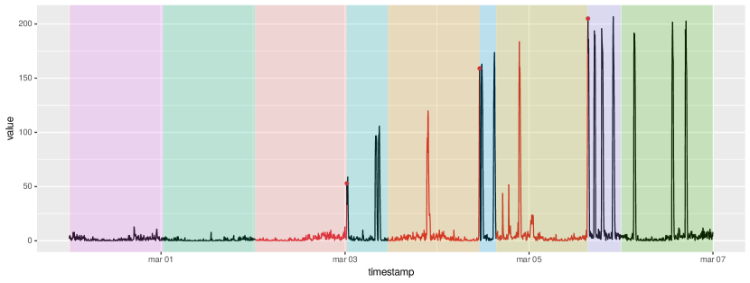
Figure 1: Interval partition of the time series based on the red-dot highlighted anomalies.

3.2 Second component: Aggregation functions and earliness-aware scoring

Once the time-stamps are aggregated into interval instances, we propose the use of a real valuated function $f$ to summarise the anomaly score provided by the algorithm $A$ for those intervals:

$$f(X_{l})=f\left(\left\{A(\mathbf{x}):\mathbf{x}\in X_{l}\right\}\right).$$ (6)

There are some suitable options for $f$, that depend on the research interest and the used algorithm. Here we include the main choices:

Average

For those algorithms that provide an anomaly score, the mean is the basic aggregator. The results are expected to be more representative for the scenarios with more instances in each interval.

CCDF

The Complementary Cumulative Density Function, with a threshold, to compute the percentage of instances with an anomaly score greater than such threshold. This aggregation function can be suitable for scenarios with less instances within each interval or for those algorithms that only provide a label instead of an anomaly score. This aggregator with a 0.5 threshold is the median aggregation function.

NAB

The Numenta weighting scheme is reformulated as another aggregation function, giving less relevance to those time-stamp instances that are too close to the event, as it is imminent and an anomaly prediction lacks use.

$$f_{NAB,w}(X_{l})=\sum_{\mathbf{x}_{j}\in X_{l}}\sigma_{w}(\operatorname{time\_until\_next\_alarm}(t_{j}))\cdot\operatorname{algorithm}(\mathbf{x_{j}}),$$

where $\sigma_{w}(t)=\frac{2}{1+e^{15t/w}}-1$. This gives a weight of near 1 for those instances further to the next event than $w$, so we can ignore the weight in the negative intervals. The 15 coefficient for the distance is derived from Numenta Anomaly Benchmark, as they use a 5 coefficient for a 3 hours window.

Filtering consideration

For those algorithms that provide an anomaly label for each instance, particularly for those situations where they provide a high rate of positive labels, the aforementioned aggregation functions may lead to a high false positive ratio. As described in the previous section, there are some options for filtering the positive instances:

Non-trigger window

A second window $w_{2}$ may be defined after each instance declared to be positive by the algorithm, within which no other positive instance is considered to the aggregation [24].

Counter

We could considered a sliding window, where only the last triggered alarm is declared as an anomaly if there were more than a certain number $K$ of alarms in such period.

The use of these functions is independent of the aggregation function and may be considered as a part of it via composition $f^{\prime}=f\circ g$, where $g$ represent a filtering function and $f$ and $f^{\prime}$ are aggregation functions.

3.3 Third component: Evaluation based in the Preceding Window ROC

ROC curve can be defined as a plot of the sensitivity versus $(1-\operatorname{specificity})$ for all possible threshold values $c$

$$\operatorname{ROC}=\left\{(P(y>c|\hat{y}=0),P(y>c|\hat{y}=1)):c\in\left(\infty,\infty\right)\right\},$$ (7)

where $y$ represents the score and $\hat{y}$ the real class. In our proposal, this definition is subject to $w$, as it determines the score $y$ through the aggregation made by $f$. The inclusion of the time as a parameter for the definition of ROC was also suggested by Heagerty et al. [25] for a different scenarios. Their work proposes an estimation for the ROC in a time-stamp posterior to a medical treatment, and the class represents the survival of the patient. This means that only the ROC computation is changed with the window length parameter, and it does not affect the label itself. Moreover, the window of study is posterior to the interest event and the class of the instance will not ever change again, unlike in our work, where the windows precedes the event and the class is negative after the event. For our evaluation framework, we propose the following definition of the pw-ROC:

Definition

Preceding Window ROC for the window length $w$:

$$\operatorname{pw-ROC}_{w}=\left\{(P(f(X)>c|X\in\mathcal{N}_{w}),P(f(X)>c|X\in\mathcal{I}_{w})):c\in\left(-\infty,\infty\right)\right\}$$ (8)

It is important to note the influence of $w$, as it affects the definition of $\mathcal{N}_{w}$ and $\mathcal{I}_{w}$. Once we have obtained the different pw-ROC curves for the desired window lengths, we can generate a ROC surface to observe the difference in the balance between precision and specificity concerning the window length. The study of this parameter allows the characterisation of the problem if the researchers do not have prior information about the possible length of the window where the anomalies can be detected in the sensors data. The AUC is expected to improve as the window length increases as there are fewer negative instances. Therefore, the window length when this performance surge happens is another element to take into account when comparing algorithmsIf there are algorithms that have a significative better AUC for shorter windows it implies that the anomalous events are detectable by these algorithms. Another option is that the surge happens in the upper limit of the range of window lengths, which may be caused if there are no negative instances, so the expert knowledge may help to avoid this issue.

The whole process is summarised in Figs. 2 to 4. From the anomaly scores or labels provided by the algorithm, depicted in Figure 2, we can filter and replicate the window partitioning according to different values of the window parameter, obtaining multiple time series partitions, illustrated by Figure 3. Then, an aggregation is performed depending on the researcher interest and a ROC surface is obtained (Figure 4).

Figure 3 also helps to explain the influence of the window length in the definition of the anomaly. For the sake of simplicity, let consider that the detection algorithm provides only $\{0,1\}$ labels and that the aggregation method is the maximum function. Then, an interval is labelled as positive if there is an anomaly predicted in such interval. As previously stated, the score is expected to increase with longer window lengths, because those undetected anomalous intervals (plotted in red and ended with a False Negative dot) could include some positive instances that were False Positives with a shorter window, as seen in the first two highlighted points in 3(a) and 3(b). Similarly, most false positives instances will be captured by true positive intervals, increasing the precision, as illustrated by the changes between 3(b) and 3(c).

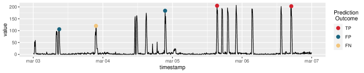
Figure 2: Anomaly scores and algorithm predictions

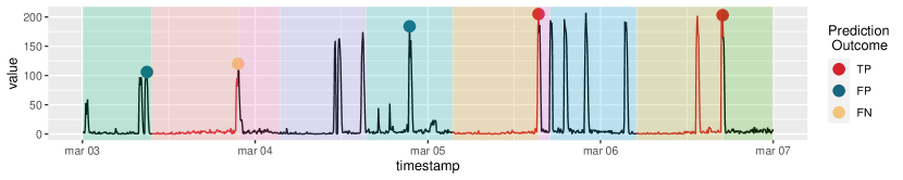
(a) 12-hours window

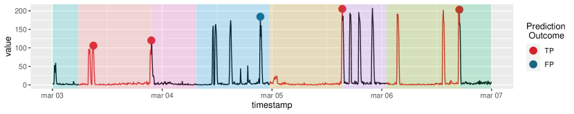
(b) 16-hours window

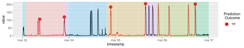
(c) 20-hours window

Figure 3: Window partitioning

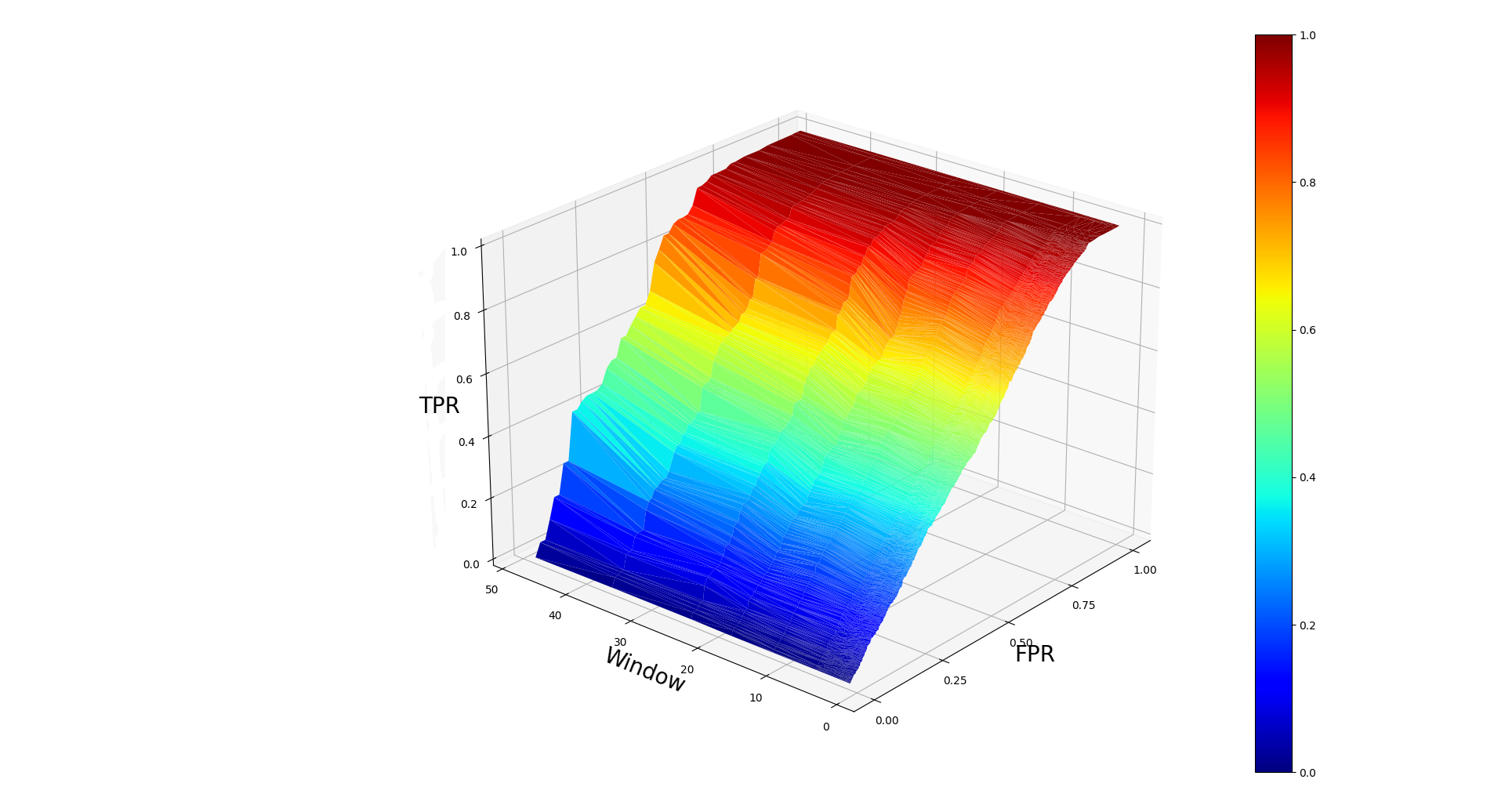
Figure 4: ROC Surface

3.4 Software

The package pwROC implements the described algorithm evaluation method. As previously stated, this package includes two versions of the method: a non distributed version, which can be installed without the Spark and pySpark dependencies, and a distributed version (the sub-module pwROCBD) for Big Data time series, which requires a working spark installation and has pySpark as python package dependency.

The package contains the functionality to preprocess the data set, filtering the instances according to the maintenances, computing a specific ROC curve for a window length or computing the ROC surface for the desired window lengths. The available aggregation functions are the mean, median, complementary cdf and the NAB weighting schema. The pwROCBD sub-module, which has the same functionality as the classic implementation, requires

By using pandas.DataFrames and pyspark.DataFrames, pwROC enables users to integrate the scoring system into their analyses. The expected data inputs are the DataFrame with the timestamp and the anomaly score, and a numpy.array with the timestamp of the start of the events of interest.

4 Case of study

In this section, we include the details of the analysis carried out with a real case of study to illustrate the appropriateness of the proposed measures and the comparison between the different modules. This analysis includes a comparison with the evaluation method for the most similar scenario found in the literature.

4.1 Description of ArcelorMittal Sensor Data

The used data have been provided by ArcelorMittal. It comes from an asset that requires permanent attention as failures occur with a high frequency. Depending on the importance of the failure, the machine can be stopped for a quick repair or need several days of reparation. The aim is to prevent these serious breakdowns through the early detection of the machine problems.

The data includes the sensor time series and some other related information (which may indicate some problem but do not imply an event of interest), e. g. failures logs, contextual information, etc. The data set consists of more than 38 million observations of 112 numeric attributes, which involve information from operational and environmental contexts.

We have preprocessed the data, scaling it to the zero-one range to prevent an artificial algorithm behaviour and discarding six features from a total of 112 due to their constant value.

4.2 Algorithms involved in the experimentation

The experimentation includes the results obtained by three unsupervised anomaly detection algorithms. These algorithms are big data redesigns of some classic anomaly detection algorithms and they are available in the AnomalyDSD Spark Package. The use of big data algorithms is derived from the volume of the used data set.

• HBOS_BD: Histogram-based Outlier Score (HBOS) anomaly detection algorithm [26]. HBOS makes a histogram for every feature of the data to assign an anomaly score according to the number of instances present in each histogram bin. Two alternatives are proposed to process the numerical features: Static, with equal-width bins, and dynamic, where the values are sorted and divided in an equal number of instances bins.

• LODA_BD: Lightweight Online Detector of Anomalies (LODA) is an ensemble-method based on the combination of random one-dimensional histograms [27]. The selection of random variables to make the histogram introduces a degree of variability, a desired feature in ensemble-based methods.

• XGBOD_BD: Extreme Gradient Boosting Outlier Detection (XGBOD)  [28] is an adaptation of XGBoost to a semi-supervised scenario. This algorithm uses unsupervised anomaly detection algorithms to obtain a representation for a supervised classifier.

In Table 2 we include the default parameters for each algorithm involved in the comparison. The best parameters for the algorithms has been determined from an hyper-parameter optimization using the Optuna Optimization Framework [29]. The used measure for the optimisation has been the proposed ROC-AUC for a 6 hours window.

Algorithm	Parameters
HBOS_BD	n_bins = 100, strategy = “static”
LODA_BD	n_bins = 100, k = 100
XGBOD_BD	detector = “LODA_BD”, n_TOS = 10, n_selected_TOS = 5, TOS_strategy = “acc”, threshold = 0.1

Table 2: Default parameter setting for the anomaly detectors

These algorithms provide anomaly scores for each instance, so the filter functions described in subsection 3.2 has not been used, although they are included in the paper to provide the mechanisms to adapt the scoring system to the researcher interests.

4.3 Results and Analysis

In Table 3 we include the AUC value for the different algorithms for some values of intervals (1, 6 and 48 hours) using the different aggregation functions. The best AUC result is highlighted in bold type. For this evaluation method, HBOS variants are in general the most effective, pointing out the general abnormality of time intervals previous to the alarms. The increasing AUC value concerning the considered period is general to all aggregation and weighting schemes. As described in Section 3, this is the expected behaviour as there are fewer windows to be considered and those previous to an incident is considered to be more abnormal. However, this increase is not guaranteed for an algorithm with random performance, and such AUCs are obtained here for certain algorithms and small windows. In this particular study case, low AUCs should not be attributed to the random performance, but to the relation between the anomalous behaviour of the machine and the timestamp where the event of interest starts.

Previous hours	Agg. function	HBOS		LODA	XGBOD
		Static	Dynamic
1	mean	0.5623	0.5760	0.5592	0.4963
	ccdf	0.4206	0.4410	0.4252	0.4510
	NAB	0.5159	0.5155	0.5155	0.4314
6	mean	0.5692	0.5886	0.5584	0.4924
	ccdf	0.4619	0.4734	0.4827	0.5092
	NAB	0.6569	0.6571	0.6557	0.6258
48	mean	0.7577	0.7334	0.6781	0.5651
	ccdf	0.5792	0.5620	0.6418	0.6094
	NAB	0.8373	0.8322	0.8332	0.8537

Table 3: AUC value for each algorithm and window length using different aggregations.

Concerning the Complementary CDF aggregation, the values show how a non-linear aggregation benefits the XGBOD algorithm. Therefore, those algorithms are more suitable for scenarios where single points may indicate an abnormal problem instead of those where the anomalies come from a general degradation of the series.

The values using the Numenta weighting mechanism are similar to the results using the mean aggregation, as we are using the same aggregation function. However, they are higher for wider windows, as the values further from the annotated event have more relative weight and we have seen that the algorithms do not perform well for narrow windows. It is important to note that XGBOD obtains the best result for the 48 hours window length with this evaluation scheme, so this algorithm also detects an abnormal general behaviour previous to the event, although only at the start of the window, which is the performance rewarded by the NAB scorer.

In 5(a), the ROC curve for the LODA algorithm with the mean aggregation for the 36 hours interval previous to an event is shown. The performance is only slightly better than a random prediction, although for this window length it could be useful in the detection of anomalies. In 5(b) we show the ROC surface of the LODA algorithm for the windows up to 48 hours previous to an incident. The aggregation method used is the mean of the score values.

In this image, the ROC surface shows that the performance is close to the random performance for windows shorter than 20 hours. We can observe that a surge in the performance when the window length is close to the upper limit, particularly in the longest window, where there is an increase in the TPR while the FPR is still low.

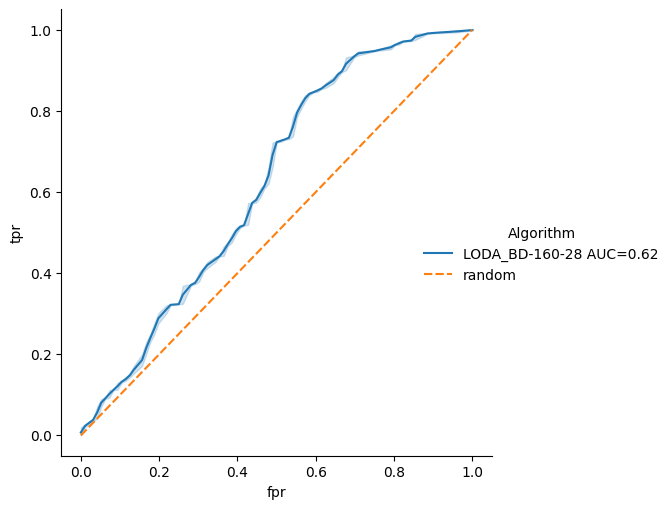
(a) Example of ROC curve for 36 hour window

(b) ROC Surface for LODA algorithm

Figure 5: ROC evaluation

We have performed statistical analysis with the results of the AUCs for the mean aggregation to compare the algorithms. This paper does not present an anomaly detection algorithm, but an evaluation framework, so the analyses are not centred on one of the algorithms. To prove that there are differences between results, we have used the Friedman test, as the results are not expected to come from Gaussian distribution due to the different window lengths [30]. The obtained $p$-value is $1.41\cdot 10^{-6}$, so we can reject the null hypothesis that represents the equivalence of the methods.

The results of a Friedman test with the Holland Post-Hoc adjust, used to search for the differences claimed by the Friedman test, are shown graphically in Figure 6. Here is shown that although HBOS variants are the algorithms with better results, we cannot discard the possibility that these differences are produced by chance. The main equivalence between the algorithms that can be discarded is between the dynamic variant of the HBOS algorithm and both LODA and XGBOD and between XGBOD and HBOS variants.

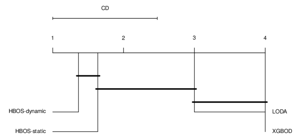
Figure 6: Critical Difference comparison plot

4.4 Comparison to Range-Based Precision and Recall

In this section, we compare our method to the range-based scoring system [21]. The goal of the comparison is to show that the concept of the preceding window ROC includes the information computed by the range-based precision and recall, with the additional benefits of the ROC curve for unsupervised scenarios. Some considerations should be made concerning this comparison:

• The range-based proposal is intended to evaluate the detection of anomalous intervals, so we have adapted the dataset, labelling as anomalous the instances previous to the events using different window lengths, similarly as in the proposed method.

• This method assumes that the outputs of the algorithm are anomaly labels, while our method works with the anomaly scores. Then, for the algorithms involved in the comparison, certain anomaly levels have been used to transform the score into dichotomic labels. For the sake of a more direct comparison, we have computed the precision, recall and $F_{1}$ at equivalent thresholds of the proposed ROC curve. It is important to note that the thresholds in the pw-ROC evaluation refer to the aggregated scores, although there is not an univocal relation between instances.

• The comparison has been made using a subset due to the computational cost of the computation of the range-based measures.

• We have used the mean aggregation for the pw-ROC measures.

• The time-based bias described in the range-based proposal has a similar goal to the NAB weights. Here we have used a flat bias in both scoring systems to focus the comparison in the evaluation of the anomaly detection.

For each algorithm, let $q_{0.05}$ and $q_{0.95}$ be the 0.05 and 0.95 quantile of the scores, respectively. Then, the labels has been assigned using a linear mapping for the thresholds:

$$\mathrm{Label}(x,\alpha)=\left\{\begin{array}[]{ll}1&\mbox{if }x\geq q_{0.05}+\alpha(q_{0.95}-q_{0.05})\\ 0&\mbox{otherwise}\end{array}\right.,$$ (9)

where $\alpha$ takes the values of $0.2,0.5$ and $0.8$. We have selected the 0.05 and 0.95 quantiles to filter the most extreme score values. Then, we have used three threshold to mimic a scenario where only an estimation of the score distribution is available.

In Table 4 we show the range-based $F_{1}$ score, using different window lengths and thresholds. With the exception of the combination of the two shortest windows and the lowest threshold, where the dynamic and static version of HBOS get the best result for the 1 and 6 hours windows, the best $F_{1}$ score is obtained in every other scenario by the XGBOD algorithm. The big differences between the scores with different anomaly thresholds imply that this scoring system rewards very positively the detection of anomalous instances without penalising the false positives, which are very likely with a low threshold. The differences with respect the pw-ROC evaluation, where XGBOD gets the worst results, can be explained by the use of a threshold, that is determinant to the detection of the anomalies. This circumstance is made clear by the following Figs. 7 to 9, which show the comparison for the precision, recall and $F_{1}$ measures between the range-based and the preceding window for each threshold and window length for both scoring methods (represented in colors).

Previous hours	Threshold	HBOS		LODA	XGBOD
		Static	Dynamic
1	0.2	0.121	0.129	0.116	0.122
	0.5	0.090	0.114	0.103	0.122
	0.8	0.089	0.071	0.075	0.122
6	0.2	0.516	0.473	0.415	0.490
	0.5	0.339	0.407	0.332	0.490
	0.8	0.188	0.168	0.175	0.490
48	0.2	0.795	0.915	0.857	0.998
	0.5	0.618	0.691	0.512	0.998
	0.8	0.245	0.274	0.289	0.998

Table 4: Range-based $F_{1}$

Figure 7 shows the precision of the algorithms for the threshold and window lengths. The results for both scoring methods are more similar for the precision measure. For the 48 window length, all the predicted anomalous intervals fall into anomalous ranges, meaning a 1 range-based precision. However, this is not the case for the pw-ROC computation of the precision, as it may be that the mean scores of some positive windows are less than the mean of instances outside the positive windows. Then, the situation here could be that positive ranges and windows contain anomalous instances, although the majority of scores are much lower.

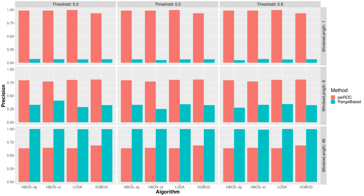
Figure 7: Preceding Window vs Range-Based Precision

The mentioned hypothesis is supported by the comparison between the range-based recall and the recall within the previous window shown in Figure 8. It is important to note that the range-based recall of the XGBOD algorithm is 1 in all the scenarios, which means that all the positive instances are labelled as anomalies for all the considered thresholds. Therefore, the determination of the anomaly threshold is for the evaluation of this algorithm, while the pw-ROC scoring system provides an evaluation more similar to the other algorithms ones. Then, for this approach, we should know the distribution of the scores and adjust the threshold accordingly, as the precision is very low for the lower window lengths. These results reinforce the hypothesis that ROC based scoring systems are fairer, as they show the effectiveness for all the possible thresholds. Another aspect that polarises the output of the ranged based evaluation for algorithms that have a narrow range of scores is the fact that the presence or absence of instances labelled as anomalies affect the evaluation of the whole interval, while the pw-ROC aggregates the information of the instances within the periods, a process that avoids the dichotomisation of the output.

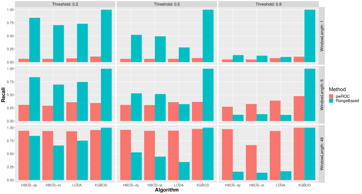
Figure 8: Preceding Window vs Range-Based Recall

The combination of the previous scores is shown in Figure 9, which depicts the comparison between the range-based $F_{1}$ score for each threshold and window length. The deepest difference here relies on the XGBOD algorithm, which performs well in terms of the pw-ROC for the lower thresholds, but obtains a near 1 range-based $F_{1}$ score for every threshold for the 48 hours window length.

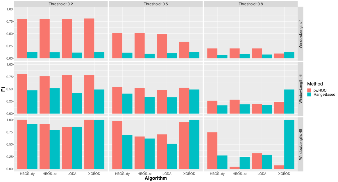
Figure 9: Preceding Window vs Range-Based F1

As mentioned before, this is a case where the good definition of the threshold is crucial, while the pw-ROC computation of the score is not affected by it, not only by being unnecessary to the computation of the curve but through the window aggregation.

Cost analysis

The alleged computational complexity of the range-based measures is $O(N_{r}\times N_{p})$, where $N_{r}$ is the number of real anomalous intervals and $N_{p}$ represents the number of predicted anomalous intervals. However, this cost omit the computation of the size of the intersection of the predicted and real anomalous intervals and the biased weight of the instances within, which could lead to a $O(n^{2})$ computational cost, where $n$ is the number of instances. The complexity of the proposed method is $O(n)$, which could be a greater number than $N_{r},N_{p}$, although our proposal is much more efficient in practice.

Table 5 shows the computational time of each evaluation method for each threshold and window length. The results included in this table are the mean computational time between the computational times for all the algorithms and it is measured in seconds. The computational cost of the range-based measure is much greater than the cost of the proposed method, especially when a larger window is considered. The increase in the computational cost needed by the range-based method for longer windows is derived from the need of computing the intersection between longer anomalous intervals. A similar circumstance happens with the 0.5 threshold, which implies a greater number of changes between normal and anomalous predicted intervals. On the contrary, the cost of the proposed method is only affected by the number of instances, as longer windows mean fewer aggregations of more instances.

WindowLength	Threshold	pwROC	RangedBased
1	0.2	0.14	146.12
	0.5	0.11	214.73
	0.8	0.09	101.24
6	0.2	0.46	233.41
	0.5	0.41	360.14
	0.8	0.29	167.15
48	0.2	0.94	17533.13
	0.5	0.88	29105.63
	0.8	0.38	12166.45

Table 5: Comparison of computational cost (sec) of evaluation methods

5 Concluding remarks

This work proposes an evaluation framework for anomaly detection for time series scenarios. This framework allows the use of AUC, an extended anomaly detection measure, for event detection regarding the uncertainty about the annotated timestamp of the event. The description of the components applied to the original time series data allows the researcher to propose new aggregation functions designed for their particular case within the proposed framework, which can lead to more appropriate conclusions. We also have adapted into the framework the well-known Numenta Anomaly Benchmark scoring system to reward the early detection of the anomalies although our definition avoids the proliferation of parameters that can obscure the meaning of the measure.

The experimentation with three different distributed algorithms for a real-world case study with the mentioned characteristics of anomaly annotation, and the comparison with a range-based scoring system, have validated the robustness of the proposal of the used metrics and methods through the description of a ROC based score instead of depending on an anomaly threshold, which could bring a more dichotomous situation. Therefore, the presented evaluation method has made viable the study of a problem of anomaly detection for time series, with both classic and Big Data implementations of the scoring method, which otherwise would have to use inappropriate or inefficient measures that could lead to wrong conclusions about the quality of the algorithms.

References

- [1] V. Chandola, A. Banerjee, V. Kumar, Anomaly detection: A survey, ACM computing surveys (CSUR) 41 (3) (2009) 15.
- [2] B. Wang, Z. Mao, Outlier detection based on a dynamic ensemble model: Applied to process monitoring, Information Fusion 51 (2019) 244–258. doi:10.1016/j.inffus.2019.02.006.
- [3] Z. Zohrevand, U. Glässer, Dynamic Attack Scoring Using Distributed Local Detectors, in: ICASSP 2020 - 2020 IEEE International Conference on Acoustics, Speech and Signal Processing (ICASSP), 2020, pp. 2892–2896. doi:10.1109/ICASSP40776.2020.9054264.
- [4] R. Noorossana, S. S. Hosseini, A. Heydarzade, An overview of dynamic anomaly detection in social networks via control charts, Quality and Reliability Engineering International 34 (4) (2018) 641–648. doi:10.1002/qre.2278.
- [5] A. Carreño, I. Inza, J. A. Lozano, Analyzing rare event, anomaly, novelty and outlier detection terms under the supervised classification framework, Artificial Intelligence Review (Oct. 2019). doi:10.1007/s10462-019-09771-y.
- [6] A. Theofilatos, G. Yannis, P. Kopelias, F. Papadimitriou, Predicting Road Accidents: A Rare-events Modeling Approach, Transportation Research Procedia 14 (2016) 3399–3405. doi:10.1016/j.trpro.2016.05.293.
- [7] R. P. Ribeiro, P. Pereira, J. Gama, Sequential anomalies: A study in the Railway Industry, Machine Learning 105 (1) (2016) 127–153. doi:10.1007/s10994-016-5584-6.
- [8] C. C. Aggarwal, Outlier Analysis, Springer-Verlag, New York, 2017.
- [9] D. Fernández-Francos, Ó. Fontenla-Romero, A. Alonso-Betanzos, One-Class Convex Hull-Based Algorithm for Classification in Distributed Environments, IEEE Transactions on Systems, Man, and Cybernetics: Systems 50 (2) (2020) 386–396. doi:10.1109/TSMC.2017.2771341.
- [10] A. L. I. Oliveira, F. R. G. Costa, C. O. S. Filho, Novelty detection with constructive probabilistic neural networks, Neurocomputing 71 (4) (2008) 1046–1053. doi:10.1016/j.neucom.2007.11.003.
- [11] M. Goldstein, S. Uchida, A Comparative Evaluation of Unsupervised Anomaly Detection Algorithms for Multivariate Data, PLOS ONE 11 (4) (2016) e0152173. doi:10.1371/journal.pone.0152173.
- [12] A. Lavin, S. Ahmad, Evaluating Real-Time Anomaly Detection Algorithms – The Numenta Anomaly Benchmark, 2015 IEEE 14th International Conference on Machine Learning and Applications (ICMLA) (Dec. 2015). doi:10.1109/icmla.2015.141.
- [13] N. Craswell, Precision at n., in: Encyclopedia of Database Systems, Springer, Berlin, Germany, 2009, pp. 2127–2128.
- [14] X. Xu, H. Liu, M. Yao, Recent Progress of Anomaly Detection, Complexity 2019 (2019) e2686378. doi:10.1155/2019/2686378.
- [15] A. Fernández, S. García, M. Galar, R. C. Prati, B. Krawczyk, F. Herrera, Learning from Imbalanced Data Sets, Springer, 2018.
- [16] J. A. Hanley, B. J. McNeil, The meaning and use of the area under a receiver operating characteristic (ROC) curve., Radiology 143 (1) (1982) 29–36. doi:10.1148/radiology.143.1.7063747.
- [17] N. Zeng, Z. Wang, Y. Li, M. Du, J. Cao, X. Liu, Time series modeling of nano-gold immunochromatographic assay via expectation maximization algorithm, IEEE Transactions on Biomedical Engineering 60 (12) (2013) 3418–3424.
- [18] N. Zeng, Z. Wang, H. Zhang, Inferring nonlinear lateral flow immunoassay state-space models via an unscented Kalman filter, Science China Information Sciences 59 (11) (2016) 112204. doi:10.1007/s11432-016-0280-9.
- [19] B. Gunay, Z. Shi, C. Yang, W. Shen, D. Darwazeh, An inquiry into the predictability of failure events in chillers and boilers, in: 2019 IEEE 15th International Conference on Automation Science and Engineering (CASE), 2019, pp. 222–227. doi:10.1109/COASE.2019.8843290.
- [20] S. Zhang, S. Bahrampour, N. Ramakrishnan, L. Schott, M. Shah, Deep learning on symbolic representations for large-scale heterogeneous time-series event prediction, in: 2017 IEEE International Conference on Acoustics, Speech and Signal Processing (ICASSP), 2017, pp. 5970–5974. doi:10.1109/ICASSP.2017.7953302.
- [21] N. Tatbul, T. J. Lee, S. Zdonik, M. Alam, J. Gottschlich, Precision and Recall for Time Series, arXiv:1803.03639 [cs]Comment: 11 pages, 32nd Conference on Neural Information Processing Systems (NeurIPS 2018), Montreal, Canada (Jan. 2019).
- [22] T. J. Lee, J. Gottschlich, N. Tatbul, E. Metcalf, S. Zdonik, Precision and Recall for Range-Based Anomaly Detection, arXiv:1801.03175 [cs] (Feb. 2018).
- [23] N. Singh, C. Olinsky, Demystifying Numenta anomaly benchmark, in: Neural Networks (IJCNN), 2017 International Joint Conference On, IEEE, 2017, pp. 1570–1577.
- [24] A. Iturria, J. Carrasco, S. Charramendieta, A. Conde, F. Herrera, Otsad: A package for online time-series anomaly detectors, Neurocomputing 374 (2020) 49–53. doi:10.1016/j.neucom.2019.09.032.
- [25] P. J. Heagerty, T. Lumley, M. S. Pepe, Time-Dependent ROC Curves for Censored Survival Data and a Diagnostic Marker, Biometrics 56 (2) (2000) 337–344. doi:10.1111/j.0006-341X.2000.00337.x.
- [26] M. Goldstein, A. Dengel, Histogram-based outlier score (hbos): A fast unsupervised anomaly detection algorithm, KI-2012: Poster and Demo Track (2012) 59–63.
- [27] T. Pevnỳ, Loda: Lightweight on-line detector of anomalies, Machine Learning 102 (2) (2016) 275–304.
- [28] Y. Zhao, M. K. Hryniewicki, XGBOD: Improving supervised outlier detection with unsupervised representation learning, in: 2018 International Joint Conference on Neural Networks (IJCNN), IEEE, 2018, pp. 1–8.
- [29] T. Akiba, S. Sano, T. Yanase, T. Ohta, M. Koyama, Optuna: A Next-generation Hyperparameter Optimization Framework, in: Proceedings of the 25th ACM SIGKDD International Conference on Knowledge Discovery & Data Mining, KDD ’19, Association for Computing Machinery, New York, NY, USA, 2019, pp. 2623–2631. doi:10.1145/3292500.3330701.
- [30] J. Carrasco, S. García, M. M. Rueda, S. Das, F. Herrera, Recent trends in the use of statistical tests for comparing swarm and evolutionary computing algorithms: Practical guidelines and a critical review, Swarm and Evolutionary Computation 54 (2020) 100665. doi:10.1016/j.swevo.2020.100665.