On the number of words
with restrictions on the number of symbols

Abstract.

We show that, in an alphabet of $\displaystyle n$ symbols, the number of words of length $\displaystyle n$ whose number of different symbols is away from $\displaystyle(1-1/e)n$, which is the value expected by the Poisson distribution, has exponential decay in $\displaystyle n$. We use Laplace’s method for sums and known bounds of Stirling numbers of the second kind. We express our result in terms of inequalities.

MSC 2020: 05A05, 05A10, 05A20

Keywords: Poisson distribution; Laplace method for sums; Stirling numbers of the second kind; Combinatorics on words.

1. Introduction and statement of results

Consider an alphabet of $\displaystyle n$ symbols and let $\displaystyle\chi^{(i)}$ be the number of symbols that appear exactly $\displaystyle i$ times in a word of length $\displaystyle m$. This can be seen as the allocation of $\displaystyle m$ balls (the positions in a word of length $\displaystyle m$) in $\displaystyle n$ bins (the $\displaystyle n$ symbols of the alphabet), which determines a total of $\displaystyle n^{m}$ allocations. When $\displaystyle m/n$ is a fixed constant $\displaystyle\lambda$,

$$\frac{1}{n}\chi^{(i)}\text{ converges in probability to }e^{-\lambda}\frac{\lambda^{i}}{i!},$$

which is the Poisson formula, the proof can be read from [6, Example III.10 and Proposition V.11].

We are interested in the case when the alphabet size $\displaystyle n$ equals the word length $\displaystyle m$, hence $\displaystyle\lambda=m/n=1$. The number of symbols that do not appear in a word of length $\displaystyle n$ is $\displaystyle\chi^{(0)}$ and its expected value is $\displaystyle n/e$. Hence, the expected number of different symbols in a word of length $\displaystyle n$ is $\displaystyle n-n/e=(1-1/e)n$. The probability that $\displaystyle\chi^{(0)}$ is equal to $\displaystyle j$ for $\displaystyle j=0,1,\ldots,n$ is expressible in terms of Stirling numbers of the second kind: the number $\displaystyle a(n,j)$ of words of length $\displaystyle n$ with exactly $\displaystyle j$ different symbols is the number of ways to choose $\displaystyle j$ out of $\displaystyle n$ elements times the number of surjective maps from a set of $\displaystyle n$ positions to a set of $\displaystyle j$ symbols. To make such a surjective map, first partition the set of $\displaystyle n$ elements into $\displaystyle j$ nonempty subsets and, in one of the $\displaystyle j!$ many ways, assign one of these subsets to each element in the set of $\displaystyle j$ elements,

$$a(n,j)=\binom{n}{j}j!\ S_{n}^{(j)},$$

where

$$S_{n}^{(j)}=\frac{1}{j!}\sum_{i=0}^{j}(-1)^{i}\binom{j}{i}(j-i)^{n}.$$

Notice that

$$\sum_{j=0}^{n}a(n,j)=n^{n}.$$

Theorem 1 is the main result of this note and shows that in an alphabet of $\displaystyle n$ symbols, the number of words of length $\displaystyle n$ with exactly $\displaystyle j$ symbols, has exponential decay in $\displaystyle n$ when $\displaystyle j$ is away from the value expected by the Poisson distribution. Precisely, Theorem 1 proves that $\displaystyle a(n,j)$, has exponential decay in $\displaystyle n$ when $\displaystyle j$ is away from $\displaystyle(1-1/e)n$. And this implies that for every positive $\displaystyle\varepsilon<1$,

$$\sum_{n\geq 1}n^{-n}\left(\sum_{j=1}^{(1-1/e-\varepsilon)n}a(n,j)+\sum_{j=(1-1/e+\varepsilon)n}^{n}a(n,j)\right)<\infty.$$

Theorem 1.

There is a function $\displaystyle\phi:(0,1)\mapsto\mathbb{R}$ such that $\displaystyle\phi(x)<1$ for every $\displaystyle x\not=1-1/e$, positive reals $\displaystyle r$ and $\displaystyle\Lambda$ both less than $\displaystyle 1$, and positive constants $\displaystyle c$ and $\displaystyle C$ satisfying the following condition: For every pair $\displaystyle n,j$ of integers with $\displaystyle 1\leq j\leq n$,

$$\displaystyle a(n,j) \displaystyle\leq\begin{cases}C\sqrt{n}\Lambda^{n}n^{n}\ \ \ &\hbox{, if }j/n\in[0,r]\cup[1-r,1]\\ C\ \phi(j/n)^{n}n^{n}\ \ \ &\hbox{, if }j/n\in[r,1-r]\\ \end{cases}$$

$$\displaystyle a(n,j) \displaystyle\geq\ (c/\sqrt{n})\,\phi(j/n)^{n}n^{n}\ \hbox{, if }j/n\in[r,1-r].$$

Precisely,

$$\displaystyle\phi:(0,1)\mapsto\mathbb{R}, \displaystyle\ \ \ \phi(x)=(e\ln(1+e^{-\delta(x)})^{-1}\varphi(x)e^{-x\delta(x)}$$

$$\displaystyle\varphi:[0,1]\mapsto\mathbb{R}, \displaystyle\ \ \ \varphi(x)=x^{-x}(1-x)^{-(1-x)},\ \varphi(0)=\varphi(1)=1$$

$$\displaystyle\delta:(0,1)\mapsto\mathbb{R}, \displaystyle\ \ \ \delta^{-1}(y)=\frac{1}{(1+e^{y})\ln(1+e^{-y})}.$$

Each of the values $\displaystyle c,C,\Lambda$ and $\displaystyle r$ in the statement of Theorem 1 can be effectively computed. Figure 1 plots the upper bound of $\displaystyle\sqrt[n]{a(n,j)}n^{-1}$ with the function $\displaystyle\phi(j/n)$ given in Theorem 1.

As a straightforward application of Theorem 1 we obtain the following.

Figure 1. On the left, the graph of $\displaystyle\phi(x)$. On the right, the points are $\displaystyle\sqrt[n]{a(n,j)}n^{-1}$ for $\displaystyle n=200$ and $\displaystyle j=0,5,10,\dots,195,200$ and the solid line is $\displaystyle\phi(j/n)$ with $\displaystyle r=0.1$ and $\displaystyle\Lambda\approx 0.701$.

Corollary 2.

For any positive real number $\displaystyle\varepsilon$ there exist positive constants $\displaystyle c$ and $\displaystyle C$ and a positive real number $\displaystyle\Lambda$ strictly less than $\displaystyle 1$ such that for every positive integers $\displaystyle n,\ell$,

$$\text{if }\ \ |\ell/n-(1-1/e)|\geq\varepsilon\ \ \text{ then }\ \ (c/\sqrt{n})\ \Lambda^{n}\leq n^{-n}\sum_{j=1}^{\ell}a(n,j)\leq Cn\sqrt{n}\ \Lambda^{n}.$$

A tail estimate is a quantification of the rate of decrease of probabilities away from the central part of a distribution. It is known that the tail of a given arbitrary discrete distribution has exponential decay if its probability generating function is analytic on a disk centered on zero and of radius greater than $\displaystyle 1$ [6, Theorem IX.3, page 627]. Theorem 1 gives, indeed, a tail estimate with exponential decay, but our methods are not analytic.

Our proof of Theorem 1 is elementary except for the estimates for Stirling numbers of the second kind that we use as a black box. We follow the principles of Laplace’s method for sums, which is useful for sums of positive terms which increase to a certain point and then decrease. For a general explanation with examples we refer to Flajolet and Sedgewick’s book [6, p.761], see [10] for a rigorous application to an hypergeometric-type series. However, we do not use the exp-log transformation to build the approximation function.

Specifically, to prove Theorem 1 we give a smooth function $\displaystyle\phi$ so that $\displaystyle\phi(j/n)^{n}$ bounds $\displaystyle a(n,j)n^{-n}$ from above and below (up to multiplicative sequences that increase or decrease slowly). We consider the ratio between $\displaystyle j$ and $\displaystyle n$. When $\displaystyle j$ is near to $\displaystyle 0$ or near to $\displaystyle n$ we use the classical upper bound of Stirling numbers of the second kind given by Rennie and Dobson [11]. When $\displaystyle j$ is not near to $\displaystyle 0$ nor near to $\displaystyle n$ we use Bender’s approximation of Stirling numbers of the second kind [2] as a black box. This approximation comes from analytic combinatorics methods and it was initially devised by Laplace, then proved by Moser and Wyman [9] and later sharpened by Bender, see also [8]. Our two choices are motivated by the comparison of bounds on Stirling numbers by Rennie-Dobson [11], Arratia and DeSalvo [1], and also a trivial bound, given in Section 2.

The approach we use in the proof of Theorem 1 was previously used by one of the authors in two different problems. In [3] it is used to estimate $\displaystyle n!\prod_{i=1}^{k}p_{i}^{j_{i}s}/j_{i}!$ where each $\displaystyle p_{i}$ is the probability of the symbol $\displaystyle i$ in an alphabet of $\displaystyle k$ elements, $\displaystyle s$ is a real number in $\displaystyle(0,1)$ and the integers $\displaystyle j_{i}$ sum up $\displaystyle n$ and $\displaystyle\sum_{i=1}^{k}ij_{i}\leq Mn$ for a fixed $\displaystyle M>1$. In [4, Remark 4.3] the same approach is used to obtain an upper bound for $\displaystyle\binom{n}{j}/j!$ when $\displaystyle n$ is fixed and $\displaystyle j$ varies. Besides, the asymptotic behavior of these quantities when $\displaystyle n$ tends to infinity was studied using a similar technique in [7].

We crossed the problem solved in the present note when studying the set $\displaystyle\mathcal{S}$ of infinite binary sequences with too many or too few, with respect to the expected by the Poisson distribution, different words of length $\displaystyle\lfloor\log n\rfloor$, counted with no overlapping in their initial segment of length $\displaystyle n\lfloor\log n\rfloor$, for infinitely many $\displaystyle n$s. Corollary 2 allows us to prove that the Lebesgue measure of this set $\displaystyle{\mathcal{S}}$ is zero, as follows. For simplicity, let $\displaystyle n$ be a power of $\displaystyle 2$ and let $\displaystyle\log$ be the logarithm in base $\displaystyle 2$. Identify the binary words of length $\displaystyle\log n$ with integers from $\displaystyle 0$ to $\displaystyle n-1$. Thus, each binary word of length $\displaystyle n\log n$ is identified with a with a word of $\displaystyle n$ integers from $\displaystyle 0$ to $\displaystyle n-1$. Notice that there are $\displaystyle 2^{n\log n}=n^{n}$ many of these binary words. Corollary 2 assumes an alphabet of $\displaystyle n$ symbols and gives an upper bound for the proportion of words of length $\displaystyle n$ having a number of different symbols away from $\displaystyle(1-1/e)n$, which is the quantity expected by the Poisson distribution. By the identification we made, this yields an upper bound of the proportion of binary words of length $\displaystyle n\log n$ having too many or too few different binary blocks with respect to what is expected by the Poisson distribution. Since this upper bound has exponential decay in $\displaystyle n$, we can apply Borel-Cantelli lemma to show that the sum, for every $\displaystyle n$, of these bounds is finite. Consequently, the Lebesgue measure of the set $\displaystyle{\mathcal{S}}$ is zero. A different proof of this result follows from the metric theorem given by Benjamin Weiss and Yuval Peres in [13] where they show that the set of Poisson generic sequences on a finite alphabet has Lebesgue measure $\displaystyle 1$. Their proof is probabilistic, with a randomized part and a concentration part.

2. On different bounds on Stirling numbers of second kind

We compare four estimates on Stirling numbers of the second kind $\displaystyle S_{n}^{(j)}$. When $\displaystyle j/n$ belongs to $\displaystyle(0,1)$, we consider a trivial bound, Rennie and Dobson’s bound [11] and Arratia and DeSalvo’s bounds [1]. When $\displaystyle j/n$ belongs to a closed interval included in $\displaystyle(0,1)$, we consider Bender’s estimate [2]. We start by giving bounds for the binomial coefficients.

2.1. Binomial coefficients

Consider the following bounds for the factorial which are consequence of the classical Stirling’s formula for the factorial, see [12],

$$n!=\sqrt{2\pi}n^{n+1/2}e^{-n+r_{n}},\ \ \ \frac{1}{12n+1}\leq r_{n}\leq\frac{1}{12n}.$$

Then, for any $\displaystyle n\geq 1$,

(1) $$\sqrt{2\pi}n^{n+1/2}e^{-n}\leq n!\leq\sqrt{2\pi}e^{1/12}n^{n+1/2}e^{-n}.$$

In the sequel we write $\displaystyle a\approx b$ to indicate that the two numbers $\displaystyle a$ and $\displaystyle b$ coincide up to the precision explicitly indicated, but they may differ in the fractional part that is not exhibited. For example, $\displaystyle\pi\approx 3.14159$. From this approximation of the factorial, we obtain bounds for the binomial coefficient that involve the following functions,

(2) $$\displaystyle\varphi:[0,1]\mapsto\mathbb{R}, \displaystyle\quad\varphi(x)=x^{-x}(1-x)^{-(1-x)},\ \varphi(0)=\varphi(1)=1;$$

$$\displaystyle\gamma:(0,1)\mapsto\mathbb{R}, \displaystyle\quad\gamma(x)=(x-x^{2})^{1/2}$$

There exist constants $\displaystyle c_{0}$ and $\displaystyle C_{0}$ such that for any pair of integers $\displaystyle n,j$ where $\displaystyle n\geq 2$ and $\displaystyle 1\leq j\leq n-1$,

$$\frac{c_{0}}{\sqrt{n}\gamma(j/n)}\varphi(j/n)^{n}\leq\binom{n}{j}\leq\frac{C_{0}}{\sqrt{n}\gamma(j/n)}\varphi(j/n)^{n}\ .$$

The constants $\displaystyle c_{0}$ and $\displaystyle C_{0}$ can be chosen as $\displaystyle c_{0}=(\sqrt{2\pi}e^{1/6})^{-1}\approx 0.33$ and $\displaystyle C_{0}=e^{1/12}(\sqrt{2\pi})^{-1}\approx 0.43$. From (1), it follows that

(3) $$\binom{n}{j}\leq e^{1/12}(\sqrt{2\pi})^{-1}\left(\frac{n}{j(n-j)}\right)^{1/2}\frac{n^{n}}{j^{j}(n-j)^{n-j}}.$$

First, notice that

$$\left(\frac{n}{j(n-j)}\right)^{1/2}=\frac{n^{1/2}}{{n}(j/n(1-j/n))^{1/2}}=\frac{1}{\sqrt{n}\gamma(j/n)}.$$

Now, we deal with the last factor of (3). The following holds:

$$\displaystyle\frac{n^{n}}{j^{j}(n-j)^{n-j}} \displaystyle=\frac{n^{n}}{n^{n}(j/n)^{j}(1-j/n)^{n-j}}$$

$$\displaystyle=\left({(j/n)^{-j/n}(1-j/n)^{-(1-j/n)}}\right)^{n}$$

$$\displaystyle=\varphi(j/n)^{n}.$$

This proves the upper bound on the binomial coefficient. The proof of the lower bound is similar, except that the factor $\displaystyle e^{1/12}$ appears twice in the denominator.

Finally, we remark that for any pair of positive integers $\displaystyle n,j$ such that $\displaystyle n\geq 2$ and $\displaystyle 1\leq j\leq n-1$, we have $\displaystyle\min\{j(n-j):1\leq j\leq n-1\}=n-1$ (this value is attained at $\displaystyle j=1$ or $\displaystyle j=n-1$). Also $\displaystyle n-1\geq n/2$ for $\displaystyle n\geq 2$. Hence,

$$\displaystyle\gamma(j/n) \displaystyle=\left(\frac{j(n-j)}{n^{2}}\right)^{1/2}\geq\left(\frac{n}{2n^{2}}\right)^{1/2}=\frac{\sqrt{2}}{2}n^{-1/2},\text{ and }$$

$$\displaystyle\gamma(j/n) \displaystyle\leq\max\{{\gamma(x):x\in[0,1]}\}=\max\{{(x-x^{2})^{1/2}:x\in[0,1]}\}\leq 1/2.$$

Thus, multiplying by $\displaystyle\sqrt{n}$,

$${\sqrt{2}}/2\leq\sqrt{n}\gamma(j/n)\leq(1/2)\sqrt{n},$$

which implies

$$\frac{2}{\sqrt{n}}\leq\frac{1}{\sqrt{n}\gamma(j/n)}\leq{\sqrt{2}}.$$

We have that $\displaystyle 2c_{0}\approx 0.67>1/2$ and $\displaystyle\sqrt{2}C_{0}\approx 0.61<1$. This shows the following inequalities, for every positive $\displaystyle n\geq 2$ and every $\displaystyle j$ such that $\displaystyle 1\leq j\leq n-1$,

(4) $$\frac{1}{{2}\sqrt{n}}\varphi(j/n)^{n}\leq\frac{2c_{0}}{\sqrt{n}}\varphi(j/n)^{n}\leq\binom{n}{j}\leq\sqrt{2}C_{0}\varphi(j/n)^{n}\leq\varphi(j/n)^{n}.$$

2.2. A trivial bound on Stirling numbers the second kind

The simplest upper bound takes just the first term of the alternating sum that defines $\displaystyle S_{n}^{(j)}$,

$$S_{n}^{(j)}\leq j^{n}/j!.$$

This upper bound appears explicitly taking just one term in Bonferroni inequalities, see [5, Section 4.7]. First remark that the upper bound given in  (1) for the factorial yields

(5) $$\frac{j^{n}}{j!}\leq\frac{j^{n}}{\sqrt{2\pi j}j^{j}e^{-j}}=\frac{1}{\sqrt{2\pi j}}\frac{n^{n-j}(j/n)^{n}e^{j}}{(j/n)^{j}}=\frac{1}{\sqrt{2\pi j}}\left(n^{1-j/n}(j/n)^{1-j/n}e^{j/n}\right)^{n}.$$

The same lines together with the lower bound for (1) give a lower bound for $\displaystyle j^{n}/j!$.

Let $\displaystyle\theta:[0,1]\mapsto\mathbb{R}$,

(6) $$\theta(x)=x^{1-x}e^{x}.$$

It follows that

$$\frac{1}{e^{1/12}\sqrt{2\pi j}}\left(n^{1-j/n}\theta(j/n)\right)^{n}\leq j^{n}/j!\leq\frac{1}{\sqrt{2\pi j}}\left(n^{1-j/n}\theta(j/n)\right)^{n}.$$

Consequently,

(7) $$S_{n}^{(j)}\leq\frac{1}{\sqrt{2\pi j}}\left(n^{1-j/n}\theta(j/n)\right)^{n}.$$

2.3. Rennie and Dobson’s bound

The following is the classsical upper bound of Stirling numbers of the second kind given by Rennie and Dobson [11], which holds for every positive $\displaystyle n$ and every $\displaystyle j$ such that $\displaystyle 1\leq j\leq n-1$,

(8) $$S_{n}^{(j)}\leq\frac{1}{2}\binom{n}{j}j^{n-j}.$$

Let $\displaystyle\eta:[0,1]\mapsto\mathbb{R}$,

(9) $$\eta(x)=x^{1-x}\varphi(x),$$

where $\displaystyle\varphi$ is defined in (2). Since $\displaystyle j^{n-j}=(n^{1-j/n}(j/n)^{1-j/n})^{n}$, the bounds on the binomial given in (4) imply

(10) $$\frac{1}{{2}\sqrt{n}}\left(n^{1-j/n}\eta(j/n)\right)^{n}\leq\binom{n}{j}j^{n-j}\leq\left(n^{1-j/n}\eta(j/n)\right)^{n}.$$

2.4. Arratia and DeSalvo’s bound

Arratia and DeSalvo [1, Theorems 5 and 6] give these bounds for $\displaystyle n\geq 3$ and $\displaystyle 1\leq j\leq n-2$,

$$\displaystyle S_{n}^{(j)}\leq \displaystyle A_{5}(n,j)$$

$$\displaystyle S_{n}^{(j)}\leq \displaystyle A_{6}(n,j)$$

where

$$\displaystyle A_{5}(n,j):= \displaystyle\binom{N}{n-j}e^{-2\mu_{5}(n,j)}\left(1+e^{2\mu_{5}(n,j)}D_{5}(n,j)\right)$$

$$\displaystyle A_{6}(n,j):= \displaystyle\frac{N^{n-j}}{(n-j)!}e^{-\mu_{6}(n,j)}\left(1+e^{\mu_{6}(n,j)}D_{6}(n,j)\right)$$

$$\displaystyle N:= \displaystyle\binom{n}{2}$$

$$\displaystyle\mu_{5}(n,j):= \displaystyle\binom{(n-j)}{2}\binom{n}{3}/\binom{N}{2}$$

$$\displaystyle\mu_{6}(n,j):= \displaystyle\binom{(n-j)}{2}\frac{n(n-1)(4n-5)}{6N^{2}}$$

$$\displaystyle d_{5}(n,j):= \displaystyle\ P+Q+(1-Q)((n-j)-2)(R+S+T)\text{ where }$$

$$\displaystyle P:=\frac{2\binom{n}{3}}{\binom{N}{2}}$$

$$\displaystyle Q:=\frac{13-12(n-j)+3(n-j)^{2}}{\binom{N}{2}}$$

$$\displaystyle R:=\frac{8\binom{n}{3}}{\binom{N}{2}}$$

$$\displaystyle S:=\frac{6\binom{n}{4}}{\binom{n}{3}(N-2)}$$

$$\displaystyle T:=\frac{1}{(N-2)}\left(\frac{5n-11}{4}\right)$$

$$\displaystyle d_{6}(n,j):= \displaystyle\ U+2(V+W+X)\text{ where }$$

$$\displaystyle U:=\frac{n(n-1)(4n-5)}{6N^{2}}$$

$$\displaystyle V:=4((n-j)-2)\frac{n(n-1)(2n-1)}{6N^{2}}$$

$$\displaystyle W:=\frac{3((n-j)-2)n(n-1)}{(4n-5)N}$$

$$\displaystyle Z:=\frac{2((n-j)-2)(2n-1)(n+1)}{(4n-5)N}$$

$$\displaystyle D_{5}(n,j):= \displaystyle\ \min\{d_{5}(n,j),2\mu_{5}(n,j)d_{5}(n,j),1\}$$

$$\displaystyle D_{6}(n,j):= \displaystyle\ \min\{(d_{6}(n,j),2\mu_{6}(n,j)d_{6}(n,j),1\}.$$

The goal of this section is to give bounds on $\displaystyle A_{5}(n,j)$ and $\displaystyle A_{6}(n,j)$ from below and above. They are displayed in Proposition 5, and the proofs of these bounds rely on Lemma 3 and Lemma 4. In the sequel when we write $\displaystyle A_{5,6}$ we denote two statements, one about $\displaystyle A_{5}$ and one about $\displaystyle A_{6}$. Similarly for $\displaystyle D_{5,6}$ and $\displaystyle\mu_{5,6}$

Lemma 3.

For any $\displaystyle n\geq 3$ and $\displaystyle 1\leq j\leq n-2$,

$$\frac{1}{{2}n^{2}}\leq e^{-\mu_{5,6}(n,j)}\left(1+e^{\mu_{5,6}(n,j)}D_{5,6}(n,j)\right)\leq 2.$$

Proof.

By definition, $\displaystyle D_{5,6}(n,j)\leq 1$, and clearly $\displaystyle\mu_{5,6}(n,j)\geq 0$, then

$$e^{-\mu_{5,6}(n,j)}\left(1+e^{\mu_{5,6}(n,j)}D_{5,6}(n,j)\right)=e^{-\mu_{5,6}(n,j)}+D_{5,6}(n,j)\leq 2.$$

To obtain a lower bound for $\displaystyle e^{-\mu_{5,6}(n,j)}+D_{5,6}(n,j)$, it suffices to bound the quantities $\displaystyle D_{5,6}(n,j)$.

Lower bound for $\displaystyle D_{5}(n,j)$. First we consider $\displaystyle\mu_{5}(n,j)$. The equality

(11) $$\binom{N}{2}=\frac{1}{2}\frac{n(n-1)}{2}\left(\frac{n(n-1)}{2}-1\right)=\frac{(n+1)n(n-1)(n-2)}{8}$$

yields

$$\mu_{5}(n,j)=\frac{2}{3}\frac{(n-j)(n-j-1)}{n+1}.$$

This quantity, $\displaystyle\mu_{5}(n,j)$, takes its minimum when $\displaystyle j=n-2$. It follows that

$$\mu_{5}(n,j)\geq\frac{1}{n}.$$

We claim that the quantity $\displaystyle d_{5}(n,j)=P+Q+(1-Q)((n-j)-2)(R+S+T)$ satisfies that

$$d_{5}(n,j)\geq P\quad\text{for any}\quad 1\leq j\leq n-2.$$

It is clear that $\displaystyle Q$ and $\displaystyle((n-j)-2)(R+S+T)$ are nonnegative. It only remains to prove that $\displaystyle 1-Q$ is nonnegative. In fact, $\displaystyle Q\leq 1/2$ for the values of $\displaystyle n$ and $\displaystyle j$ under consideration. To prove that, first, we complete squares and apply (11); then we take $\displaystyle j=1$, and finally, we maximize over over $\displaystyle n$ to obtain the last inequality,

$$Q=8\frac{3((n-j)-2)^{2}+1}{(n+1)n(n-1)(n-2)}\leq 8\frac{3(n-3)^{2}+1}{(n+1)n(n-1)(n-2)}\leq\frac{1}{2}.$$

Finally,

$$d_{5}(n,j)\geq P=2\frac{\binom{n}{3}}{\binom{N}{2}}=\frac{8}{3(n+1)}\geq\frac{1}{n}.$$

From the last lower bound and the bound $\displaystyle\mu_{5}(n,j)\geq 1/n$, we get the following:

$$D_{5}(n,j):=\min\left(d_{5}(n,j),2\mu_{5}(n,j)d_{5}(n,j),1\right)\geq\min\left(\frac{1}{n},\frac{2}{n^{2}},1\right)\geq\frac{1}{n^{2}}.$$

Lower bound for $\displaystyle D_{6}(n,j)$. First we consider $\displaystyle\mu_{6}(n,j)$. By definition, $\displaystyle N=\binom{n}{2}$.
It turns out that for every $\displaystyle n\geq 3$ and $\displaystyle j$ such that $\displaystyle 1\leq j\leq n-2$,

$$\mu_{6}(n,j)=\binom{(n-j)}{2}\frac{n(n-1)(4n-5)}{6N^{2}}=\frac{1}{3}\frac{(n-j)(n-j-1)(4n-5)}{n(n-1)}\geq\frac{1}{n}.$$

All the terms involved in the sum defining $\displaystyle d_{6}(n,j)$ are non-negative. Hence,

$$d_{6}(n,j){\geq U=}\frac{n(n-1)(4n-5)}{6N^{2}}=\frac{2}{3}\frac{4n-5}{n(n-1)}\geq\frac{2}{3n}.$$

Finally, the following holds and completes the proof of this lemma.

$$D_{6}(n,j):=\min\left(d_{6}(n,j),2\mu_{6}(n,j)d_{6}(n,j),1\right)\geq\min\left(\frac{2}{3n},\frac{4}{3n^{2}},1\right)\geq\frac{1}{2n^{2}}.$$

∎

Let $\displaystyle\kappa$ be the map from $\displaystyle[0,1]$ to $\displaystyle\mathbb{R}$ given by

(12) $$\kappa(x)=(e/2)^{1-x}(1-x)^{-(1-x)},\ \ \kappa(1)=1.$$

Lemma 4.

For any $\displaystyle n\geq 3$ and $\displaystyle j$ with $\displaystyle 1\leq j\leq n-2$, the following holds

(13) $$\displaystyle\frac{{e^{-2}}}{{2}\sqrt{n(n-1)}}\left(n^{1-j/n}\kappa(j/n)\right)^{n} \displaystyle\leq\binom{N}{n-j}\leq\left(n^{1-j/n}\kappa(j/n)\right)^{n},$$

(14) $$\displaystyle\frac{1}{4\sqrt{2\pi}\sqrt{n}}\left(n^{1-j/n}\kappa(j/n)\right)^{n} \displaystyle\leq\frac{N^{n-j}}{(n-j)!}\leq\frac{{1}}{\sqrt{2\pi}}\left(n^{1-j/n}\kappa(j/n)\right)^{n}.$$

Proof.

We start by proving Inequality (13). With the bounds given for the binomial coefficients in (4), the following holds

(15) $$\frac{1}{2\sqrt{N}}\varphi((n-j)/N)^{N}\leq\binom{N}{n-j}\leq\varphi((n-j)/N)^{N}$$

with $\displaystyle\varphi(x)=x^{-x}(1-x)^{-(1-x)}$, for any $\displaystyle n\geq 3$ and $\displaystyle 1\leq j\leq n-2$. The expression $\displaystyle\varphi((n-j)/N)^{N}$ has two factors, the first one corresponds to $\displaystyle x^{-x}$ and the second one corresponds to $\displaystyle(1-x)^{1-x}$. We replace $\displaystyle N$ by $\displaystyle n(n-1)/2$ only in the first factor. The exponent of the second factor is multiplied and divided by $\displaystyle{N}/({n-j})$. This leads to the following equality

$$\varphi\left(\frac{(n-j)}{N}\right)^{N}=n^{n-j}\left(1-\frac{1}{n}\right)^{n-j}\left(2\left(1-\frac{j}{n}\right)\right)^{-(n-j)}b(n,j)$$

with

(16) $$b(n,j)=\left(\left(1-\frac{n-j}{N}\right)^{\frac{N}{n-j}}\right)^{-(n-j)+\frac{(n-j)^{2}}{N}}.$$

Let $\displaystyle c(n,j)$ be defined as

$$c(n,j)=\left(1-\frac{1}{n}\right)^{n-j}b(n,j).$$

The right hand side of the equality before (16) is the product of four factors. We leave the first and the third as they are. We deal with the second and the fourth. The factor $\displaystyle(1-1/n)^{n-j}$ satisfies

(17) $$e^{-1}\leq\left(1-\frac{1}{n}\right)^{n-1}\leq\left(1-\frac{1}{n}\right)^{n-j}\leq 1.$$

The right hand side inequality is due to the fact that $\displaystyle 1-1/n\leq 1$. The left hand side inequality is due to the fact that $\displaystyle(1-{1}/{n})^{n-1}$ decreases towards its limit as $\displaystyle n\to\infty$.

We study $\displaystyle b(n,j)$, defined in (16). First, we use the classical inequality

$$-x-x^{2}\leq\ln(1-x)\leq-x\quad(0<x\leq 2/3).$$

After multiplying by $\displaystyle 1/x$ and taking powers, we get

(18) $$e^{-1-x}\leq(1-x)^{1/x}\leq e^{-1}\quad(0<x\leq 2/3).$$

Observe that, for $\displaystyle j\geq 1$,

$$\frac{n-j}{N}=\frac{2(n-j)}{n(n-1)}\leq\frac{2}{n}.$$

Notice that $\displaystyle 0<({n-j})/{N}\leq 2/3$ since $\displaystyle n\geq 3$. This allows us to replace $\displaystyle x$ by $\displaystyle(n-j)/N$ in (18). It turns out that

$$e^{-1-(\frac{n-j}{N})}\leq\left(1-\frac{n-j}{N}\right)^{\frac{N}{n-j}}\leq e^{-1}.$$

To obtain $\displaystyle b(n,j)$, consider the previous expressions to the power $\displaystyle-(n-j)+{(n-j)^{2}}/{N}$. With our bound on $\displaystyle(n-j)/N$, the exponent of the left hand side satisfies

$$\left(-1-\frac{n-j}{N}\right)\left(-(n-j)+\frac{(n-j)^{2}}{N}\right)=(n-j)-\frac{(n-j)^{3}}{N^{2}}\geq(n-j)-1.$$

Finally,

(19) $$e^{-1}e^{(n-j)}\leq b(n,j)\leq e^{(n-j)-\frac{(n-j)^{2}}{N}}\leq e^{(n-j)}.$$

From Inequalities (17) and (19), it follows that $\displaystyle c(n,j)e^{-(n-j)}$ takes values in $\displaystyle[e^{-2},1]$ and the following holds

$$\displaystyle\varphi\left(\frac{(n-j)}{N}\right)^{N} \displaystyle=c(n,j)n^{n-j}\left(2\left(1-\frac{j}{n}\right)\right)^{-(n-j)}$$

$$\displaystyle=c(n,j)e^{-(n-j)}\left(n^{1-j/n}\kappa(j/n)\right)^{n}.$$

To end the proof of Inequality (13) consider Inequality (15) together with the fact that $\displaystyle N=n(n-1)/2$.

Proof of Inequality (14). Approximating the factorial by (1); extracting $\displaystyle n$ as a common factor in $\displaystyle(n-j)^{n-j}$, in $\displaystyle(n-1)^{n-j}$, and in $\displaystyle(n-1)^{n-j}$; and writing the final expression as an $\displaystyle n$-th power (similarly to what it is done in (5)), we get

$$\displaystyle\frac{N^{n-j}}{(n-j)!} \displaystyle\leq\frac{n^{n-j}(n-1)^{n-j}}{2^{n-j}}\frac{e^{n-j}}{\sqrt{2\pi(n-j)}(n-j)^{n-j}}$$

$$\displaystyle=\frac{(1-1/n)^{n-j}}{\sqrt{2\pi(n-j)}}\left(n^{1-j/n}\kappa(j/n)\right)^{n}.$$

We obtain the lower bound similarly,

$$\frac{N^{n-j}}{(n-j)!}\geq e^{-1/12}\frac{(1-1/n)^{n-j}}{\sqrt{2\pi(n-j)}}\left(n^{1-j/n}\kappa(j/n)\right)^{n}.$$

Finally, with Inequality (17), and since $\displaystyle 1\leq n-j\leq n$, we obtain the bounds

$$\frac{1}{4\sqrt{2\pi n}}\leq\frac{e^{-1-1/12}}{\sqrt{2\pi n}}\leq\frac{(1-1/n)^{n-j}}{\sqrt{2\pi(n-j)}}\leq\frac{1}{\sqrt{2\pi}}$$

that prove the estimates on $\displaystyle{N^{n-j}}/(n-j)!$. ∎

The next Proposition 5 is a direct consequence of Lemmas 3 and 4. Recall that $\displaystyle\kappa:[0,1]\to\mathbb{R}$ defined in (12), $\displaystyle\kappa(x)=(e/2)^{1-x}(1-x)^{-(1-x)},\ \ \kappa(1)=1$.

Proposition 5.

For any $\displaystyle n\geq 3$ and $\displaystyle 1\leq j\leq n-2$,

(20) $$\frac{e^{-2}}{4n^{3}}\left(n^{1-j/n}\kappa(j/n)\right)^{n}\leq A_{5,6}(n,j)\leq 2\left(n^{1-j/n}\kappa(j/n)\right)^{n}.$$

Proof.

Lemma 3 proves that, for any $\displaystyle n\geq 3$ and $\displaystyle 1\leq j\leq n-2$,

$$\frac{1}{2n^{2}}\leq e^{-\mu_{5,6}(n,j)}\left(1+e^{\mu_{5,6}(n,j)}D_{5,6}(n,j)\right)\leq 2.$$

Then,

$$\displaystyle\frac{1}{{2}n^{2}}\binom{N}{n-j}\leq \displaystyle A_{5}(n,j) \displaystyle\leq 2\binom{N}{n-j},$$

$$\displaystyle\frac{1}{2n^{2}}\frac{N^{n-j}}{(n-j)!}\leq \displaystyle A_{6}(n,j) \displaystyle\leq 2\frac{N^{n-j}}{(n-j)!}.$$

Lemma 4 provides us bounds on the terms involving combinatorials and factorials and gives

$$\displaystyle\frac{e^{-2}}{2\sqrt{n(n-1)}}\left(n^{1-j/n}\kappa(j/n)\right)^{n} \displaystyle\leq\binom{N}{n-j}\leq\left(n^{1-j/n}\kappa(j/n)\right)^{n},$$

$$\displaystyle\frac{1}{4\sqrt{2\pi}\sqrt{n}}\left(n^{1-j/n}\kappa(j/n)\right)^{n} \displaystyle\leq\frac{N^{n-j}}{(n-j)!}\leq\frac{1}{\sqrt{2\pi}}\left(n^{1-j/n}\kappa(j/n)\right)^{n}.$$

Finally,

$$\displaystyle\frac{e^{-2}}{4n^{3}}\left(n^{1-j/n}\kappa(j/n)\right)^{n} \displaystyle\leq A_{5}(n,j)\leq 2\left(n^{1-j/n}\kappa(j/n)\right)^{n},$$

$$\displaystyle\frac{1}{8\sqrt{2\pi}n^{2}\sqrt{n}}\left(n^{1-j/n}\kappa(j/n)\right)^{n} \displaystyle\leq A_{6}(n,j)\leq\frac{2}{\sqrt{2\pi}}\left(n^{1-j/n}\kappa(j/n)\right)^{n}.$$

Combining both inequalities, Proposition 5 follows. ∎

2.5. Bender’s estimate

The notation $\displaystyle r_{n}\sim s_{n}$ indicates that $\displaystyle\lim_{n\to\infty}r_{n}/s_{n}=1$ when $\displaystyle n\to\infty$. Bender [2] establishes that for any real number $\displaystyle r$ such that $\displaystyle 0<r<1/2$, then

$$S_{n}^{(j)}\sim\frac{n!e^{-\alpha j}}{j!\rho^{n+1}(1+e^{\alpha})\sigma\sqrt{2\pi n}}$$

uniformly for $\displaystyle j/n\in[r,1-r]$, where $\displaystyle\alpha$ is such that

$$\displaystyle\frac{n}{j} \displaystyle=(1+e^{\alpha})\ln(1+e^{-\alpha})$$

and

$$\displaystyle\rho \displaystyle=\ln(1+e^{-\alpha}),$$

$$\displaystyle\sigma^{2} \displaystyle=\left(\frac{j}{n}\right)^{2}\big{(}1-e^{\alpha}\ln(1+e^{-\alpha})\big{)}.$$

We introduce two functions to describe the behavior of $\displaystyle S_{n}^{(j)}$ in terms of $\displaystyle j/n$ (see Fig. 2),

(21) $$\displaystyle\psi:(0,1)\mapsto\mathbb{R}, \displaystyle\psi(x)= \displaystyle\frac{e^{-((1-x)+x\delta(x))}}{x^{x}\ln(1+e^{-\delta(x)})}$$

$$\displaystyle\mu:(0,1)\mapsto\mathbb{R}, \displaystyle\mu(x)= \displaystyle\left(x(1-e^{\delta(x)}\ln(1+e^{-\delta(x)}))\right)^{1/2}$$

where $\displaystyle\delta:(0,1)\mapsto\mathbb{R}$ is defined by

(22) $$\delta^{-1}(y)=\frac{1}{(1+e^{y})\ln(1+e^{-y})}.$$

The next lemma rephrases Bender’s estimate using $\displaystyle\psi(j/n)$ and $\displaystyle\mu(j/n)$.

Lemma 6.

For any positive real number $\displaystyle r$ such that $\displaystyle 0<r<1/2$ and for any real number $\displaystyle C>1$ there exists an integer $\displaystyle n_{0}=n_{0}(r,C)\geq 2$ such that for every integer $\displaystyle n\geq n_{0}$ and for every integer $\displaystyle j$ with $\displaystyle 1\leq j\leq n-1$ and $\displaystyle j/n\in[r,1-r]$.

$$\frac{{e^{-1/12}}}{C\sqrt{2\pi n}\mu(j/n)}\left(n^{1-j/n}\psi(j/n)\right)^{n}\leq S_{n}^{(j)}\leq\frac{e^{1/12}C}{\sqrt{2\pi n}\mu(j/n)}\left(n^{1-j/n}\psi(j/n)\right)^{n}.$$

Proof.

Observe that

$$(1+e^{\alpha})\rho\sigma=\big{(}1-e^{\alpha}\ln(1+e^{-\alpha})\big{)}^{1/2}.$$

Thus, Bender’s estimate implies that for any $\displaystyle r$ with $\displaystyle 0<r<1/2$ and for any $\displaystyle C>1$ there exists $\displaystyle n_{0}=n_{0}(r,C)$ such that for any pair of positive integers $\displaystyle n,j$, with $\displaystyle n\geq n_{0}$ and $\displaystyle j/n\in[r,1-r]$,

(23) $$\frac{1}{C}T_{\alpha}(n,j)\leq S_{n}^{(j)}\leq CT_{\alpha}(n,j)$$

where

$$T_{\alpha}(n,j)=\frac{n!}{j!}\frac{e^{-\alpha j}}{\rho^{n}(1-e^{\alpha}\ln(1+e^{-\alpha}))^{1/2}\sqrt{2\pi n}}.$$

Using (1) we have

$${e^{-1/12}}e^{j-n}\frac{\sqrt{n}}{\sqrt{j}}\frac{n^{n}}{j^{j}}\leq\frac{n!}{j!}\leq e^{1/12}e^{j-n}\frac{\sqrt{n}}{\sqrt{j}}\frac{n^{n}}{j^{j}}.$$

We remark that

$$e^{j-n}\frac{n^{n}}{j^{j}}=\left(e^{-(1-j/n)}\left(j/n\right)^{-j/n}\right)^{n}.$$

Then, using the expressions for $\displaystyle\psi(n/j)$ and $\displaystyle\mu(j/n)$,

$$\frac{e^{-1/12}}{\sqrt{2\pi n}\mu(j/n)}\left(n^{\frac{(n-j)}{n}}\psi(j/n)\right)^{n}\leq T_{\alpha}(n,j)\leq\frac{e^{1/12}}{\sqrt{2\pi n}\mu(j/n)}\left(n^{\frac{(n-j)}{n}}\psi(j/n)\right)^{n}.$$

Combining these inequalities with (23) we obtain the wanted result. ∎

Figure 2. Graphs of $\displaystyle\psi(x)$ and $\displaystyle\mu(x)$.

The functions $\displaystyle\psi(x)$ and $\displaystyle\mu(x)$ are smooth and concave in the open interval $\displaystyle(0,1)$. The function $\displaystyle\delta^{-1}(y)$ is increasing and

$$\lim_{x\to 0^{+}}\delta(x)=-\infty\hbox{ and }\lim_{x\to 1^{-}}\delta(x)=+\infty.$$

From this, it is clear that $\displaystyle\lim_{x\to 0^{+}}\psi(x)=0$, $\displaystyle\lim_{x\to 1^{-}}\psi(x)=1$, and $\displaystyle\lim_{x\to 0^{+}}\mu(x)=$ $\displaystyle\lim_{x\to 1^{-}}\mu(x)=0$. Then, the bounds given in Lemma 6 become indeterminate when $\displaystyle j/n$ is near $\displaystyle 0$ or $\displaystyle 1$. This is why $\displaystyle j/n$ must be in a central interval in $\displaystyle(0,1)$.

The next corollary is a straightforward consequence of Lemma 6 and the fact that $\displaystyle\mu(x)$ is uniformly bounded on any closed interval included in $\displaystyle(0,1)$. The constants $\displaystyle c_{1}$ and $\displaystyle C_{1}$ in the statement of Corollary 7 can be chosen as the minimum and maximum values of $\displaystyle\{\mu(x):x\in[r,1-r]\}$.

Corollary 7.

For any positive real number $\displaystyle r$ such that $\displaystyle 0<r<1/2$, there exist $\displaystyle c_{1}$ and $\displaystyle C_{1}$ such that for every pair of positive integers $\displaystyle n,j$ with $\displaystyle j/n\in[r,1-r]$ we have

(24) $${e^{-1/12}}\frac{c_{1}}{\sqrt{2\pi n}}\left(n^{1-j/n}\psi(j/n)\right)^{n}\leq S_{n}^{(j)}\leq e^{1/12}\frac{C_{1}}{\sqrt{2\pi n}}\left(n^{1-j/n}\psi(j/n)\right)^{n}.$$

2.6. A plot

The four upper bounds given in (7), (10), (20) and (24) are of the form

$$S_{n}^{(j)}\leq n^{n-j}\text{\tt bound}$$

In order to visualize them we divide both sides by $\displaystyle n^{n-j}$ and we take $\displaystyle n$-th root in both sides.

$$\left(S_{n}^{(j)}/n^{n-j}\right)^{1/n}\leq\text{\tt bound}^{1/n}$$

In the four cases bound^1/n is of the form

$$\text{\tt expression}^{1/n}\left(f^{n}\right)^{1/n},$$

where expression^1/n goes to $\displaystyle 1$ as $\displaystyle n$ goes to infinity and $\displaystyle f$ is either $\displaystyle\theta$, $\displaystyle\eta$, $\displaystyle\kappa$ or $\displaystyle\psi$. Thus, we ignore expression^1/n. Figure 3 plots the following:

In dotted line, the exact value
	$\displaystyle\displaystyle\widehat{S}_{n}^{(j)}=({S}_{n}^{(j)}/n^{n-j})^{1/n}.$
The graphic of the function $\displaystyle\theta$ involved in the trivial bound
	$\displaystyle\displaystyle\widehat{S}_{n}^{(j)}\leq\frac{1}{(\sqrt{2\pi j})^{1/n}}\theta(j/n),\text{ where $\displaystyle\theta(x)$ is given in~{}\eqref{theta}.}$
The graphic of the function $\displaystyle\eta$ involved in Rennie and Dobson’s bound
	$\displaystyle\displaystyle\widehat{S}_{n}^{(j)}\leq\frac{1}{2^{1/n}}\eta(j/n),\text{ where $\displaystyle\eta(x)$ is given in~{}\eqref{eta}.}$
The graphic of the function $\displaystyle\kappa$ involved in Arratia and DeSalvo’s bound
	$\displaystyle\displaystyle\widehat{S}_{n}^{(j)}\leq{2}^{1/n}\kappa(j/n),\text{ where $\displaystyle\kappa(x)$ is given in~{}\eqref{kappa}.}$
In stroke gray line, Bender’s estimate
	$\displaystyle\displaystyle\widehat{S}_{n}^{(j)}\leq\left(e^{1/12}\frac{C_{1}}{\sqrt{2\pi n}}\right)^{1/n}\psi(j/n),$
	where $\displaystyle\psi(x)$ is given in (21) and $\displaystyle C_{1}$ in Corollary 7,
	with $\displaystyle j/n\in[r,1-r]$ for any real $\displaystyle r$ such that $\displaystyle 0<r<1/2$.
	The constant $\displaystyle C_{1}$ depends on $\displaystyle r$. In the plot of Figure 3, $\displaystyle r=0.1$.

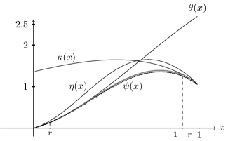
Figure 3. Comparison of the normalized Stirling numbers of the second kind $\displaystyle\widehat{S}_{n}^{(j)}=({S}_{n}^{(j)}/n^{n-j})^{1/n}$ (in dotted line), for $\displaystyle n=100$ and $\displaystyle j=1,..,100$, with the four estimates (in solid lines).

3. Application to our problem

For the proof of Theorem 1 we must give an upper bounds of $\displaystyle a(n,j)$, which is always a positive term. Since $\displaystyle a(n,j)=\binom{n}{j}j!\ S_{n}^{(j)}$, we can use upper bounds for the Stirling numbers of the second kind. We choose Rennie and Dobson’s bound in the case $\displaystyle j/n$ is near $\displaystyle 0$ or $\displaystyle 1$, and the bound originated in Bender’s estimate when $\displaystyle j/n$ is in $\displaystyle[1/r,1-1/r]$, for $\displaystyle r>0$.

3.1. When the ratio $\displaystyle j/n$ is near $\displaystyle 0$ or $\displaystyle 1$

The next lemma expresses this bound in terms of the ratio $\displaystyle j/n$ with the help of the function

(25) $$\nu:[0,1]\to\mathbb{R},\quad\nu(x)=x\ e^{-x}\varphi(x)^{2},$$

where $\displaystyle\varphi(x)$ is defined in (2).

Lemma 8.

For any pair of positive integers $\displaystyle n,j$ such that $\displaystyle n\geq 1$ and $\displaystyle 1\leq j\leq n-1$,

$$a(n,j)n^{-n}\leq\sqrt{j}\,\nu(j/n)^{n}.$$

Proof.

Recall that $\displaystyle a(n,j)=\binom{n}{j}j!\ S_{n}^{(j)}$. Rennie and Dobson’s upper bound (8) for $\displaystyle S_{n}^{(j)}$ yields

$$a(n,j)\leq\frac{1}{2}\binom{n}{j}^{2}j!j^{n-j}.$$

We apply the estimates (1) for the factorial. Then we use the upper bound for the binomial coefficient given in (4) that involves the constant $\displaystyle C_{0}=e^{1/12}(\sqrt{2\pi})^{-1}$, which yields

$$\displaystyle\frac{1}{2}\binom{n}{j}^{2}j!j^{n-j}\leq \displaystyle\frac{1}{2}(\sqrt{2}C_{0})^{2}e^{1/12}\sqrt{2\pi}\sqrt{j}\varphi(j/n)^{2}e^{-j}j^{n}$$

$$\displaystyle\leq \displaystyle\frac{e^{1/4}}{\sqrt{2\pi}}\sqrt{j}\,\nu(j/n)^{n}$$

$$\displaystyle\leq \displaystyle\sqrt{j}\,\nu(j/n)^{n}.$$

∎

The function $\displaystyle\nu(x)$ is smooth and concave, $\displaystyle\nu(0)=0$, and $\displaystyle\nu(1)=e^{-1}$. The bound given in Lemma 8 is tight when $\displaystyle j/n$ is near $\displaystyle 0$ or $\displaystyle 1$. However, it is not good when $\displaystyle j/n$ takes values in middle of the interval $\displaystyle[0,1]$. In fact, this bound satisfies $\displaystyle\sqrt{j}(\nu(1/2))^{n}\geq\sqrt{j}(1.1)^{n}>1$ but we know that $\displaystyle n^{-n}a(n,j)\leq 1$ for any choice of $\displaystyle j$ and $\displaystyle n$. This leads us to consider the only two real numbers $\displaystyle x_{0}$ and $\displaystyle x_{1}$ in $\displaystyle[0,1]$ for which $\displaystyle\nu(x_{0})=\nu(x_{1})=1$ and $\displaystyle x_{0}<x_{1}$. These numbers are $\displaystyle x_{0}\approx 0.387$ and $\displaystyle x_{1}\approx 0.790$. Figure 4 displays the graphs of $\displaystyle\nu(x)$ and $\displaystyle\varphi(x)$.

Figure 4. Graphs of functions $\displaystyle\nu(x)$ and $\displaystyle\varphi(x)$.

Lemma 9.

Let $\displaystyle x_{0}$ and $\displaystyle x_{1}$ be such that $\displaystyle 0<x_{0}<x_{1}<1$ and $\displaystyle\nu(x_{0})=\nu(x_{1})=1$. For any pair of real numbers $\displaystyle r_{0}$ and $\displaystyle r_{1}$ such that $\displaystyle 0<r_{0}<x_{0}$ and $\displaystyle x_{1}<r_{1}<1$ there exists a real number $\displaystyle\Lambda$ less than $\displaystyle 1$, such that for every positive integer $\displaystyle n$,

$$n^{-n}a(n,j)\leq\sqrt{n}\Lambda^{n}\hbox{, if }j/n\in[0,r_{0}]\cup[r_{1},1].$$

Proof.

Lemma 8 says that $\displaystyle a(n,j)n^{-n}\leq\sqrt{j}\nu(j/n)^{n}$. The function $\displaystyle\nu(x)$ is smooth and concave with $\displaystyle\nu(0)=0$, and $\displaystyle\nu(1)=e^{-1}$. This implies the existence of unique points $\displaystyle x_{0}$ and $\displaystyle x_{1}$ such that $\displaystyle 0<x_{0}<x_{1}<1$ and $\displaystyle\nu(x_{0})=\nu(x_{1})=1$. Fix $\displaystyle r_{0}$ and $\displaystyle r_{1}$ such that $\displaystyle 0<r_{0}<x_{0}$ and $\displaystyle x_{1}<r_{1}<1$. Necessarily, $\displaystyle\nu(r_{0})<1$ and $\displaystyle\nu(r_{1})<1$. Let $\displaystyle\Lambda_{0}=\nu(r_{0})$ and $\displaystyle\Lambda_{1}=\nu(r_{1})$. If $\displaystyle j/n\in[0,r_{0}]$ then

$$\nu(j/n)\leq\max\{\nu(x):x\in[0,r_{0}]\}\leq\Lambda_{0}.$$

Similarly, if $\displaystyle j/n\in[r_{1},1]$, we have $\displaystyle\nu(j/n)\leq\Lambda_{1}$. Taking $\displaystyle\Lambda=\max\{\Lambda_{0},\Lambda_{1}\}$, the lemma is proved. ∎

Example:

The choice $\displaystyle r_{0}=0.1$ yields $\displaystyle\Lambda_{0}\approx 0.173$, and $\displaystyle r_{1}=0.9$ yields $\displaystyle\Lambda_{1}\approx 0.701$. In Figure 1, the value of $\displaystyle\Lambda$ equals the maximum between the approximations of $\displaystyle\Lambda_{0}$ and $\displaystyle\Lambda_{1}$.

3.2. When the ratio $\displaystyle j/n$ is not near $\displaystyle 0$ nor $\displaystyle 1$

We introduce the function

(26) $$\phi:(0,1)\mapsto\mathbb{R},\ \ \ \ \phi(x)=(e\ln(1+e^{-\delta(x)}))^{-1}\varphi(x)e^{-x\delta(x)}$$

where $\displaystyle\varphi(x)$ is defined in (2) and $\displaystyle\delta(x)$ is defined in  (22).

Lemma 10.

Consider the constants $\displaystyle c_{1}$ and $\displaystyle C_{1}$ in Corollary 7. For any real number $\displaystyle r$ such that $\displaystyle 0<r<1/2$, and for any pair of positive integers $\displaystyle n,j$ such that $\displaystyle j/n\in[r,1-r]$

$$\frac{{e^{-1/6}}c_{1}}{\sqrt{2\pi(n-j)}}\phi(j/n)^{n}\leq n^{-n}a(n,j)\leq\frac{e^{1/6}C_{1}}{\sqrt{2\pi(n-j)}}\phi(j/n)^{n}.$$

Proof.

Write $\displaystyle a(n,j)=S_{n}^{(j)}n!/(n-j)!$, then use Stirling estimates  (1) for the factorial, apply Corollary 7 and use the definition of $\displaystyle\varphi(x)$ given in (2). ∎

The function $\displaystyle\phi(x)$ is displayed in Figure 1. It is smooth, concave, $\displaystyle\phi(0)=0$ and $\displaystyle\phi(1)=e^{-1}$. The auxiliary function $\displaystyle\delta(x)$ takes the value $\displaystyle-\ln(e-1)$ at $\displaystyle x=1-1/e$ and then, $\displaystyle\phi(1-1/e)=1$. This value is the maximum of $\displaystyle\phi(x)$ because the lower bound given in Lemma 10 implies that $\displaystyle\phi(x)\leq 1$ for $\displaystyle x\in(0,1)$.

3.3. Proofs of Theorem 1 and Corollary 2

Theorem 1 considers the ratio between $\displaystyle j$ and $\displaystyle n$. The proof combines the two cases we just studied: when $\displaystyle j/n$ is near $\displaystyle 0$ or $\displaystyle 1$, and when $\displaystyle j/n$ is in a central interval away from $\displaystyle 0$ and $\displaystyle 1$.

Proof of Theorem 1.

Consider the function $\displaystyle\nu$ given in (25). Pick numbers $\displaystyle x_{0}$ and $\displaystyle x_{1}$ such that $\displaystyle 0<x_{0}<x_{1}<1$ and $\displaystyle\nu(x_{0})=\nu(x_{1})=1$. Take any $\displaystyle r\in(0,1/2)$ so that $\displaystyle r\leq\max\{x_{0},1-x_{1}\}$. If $\displaystyle j/n\in[r,1-r]$ apply Lemma 10. Otherwise, apply Lemma 9. ∎

The proof of Corollary 2 is immediate from the statement of Theorem 1.

Proof of Corollary 2.

The result is a direct application of Theorem 1 because

$$\max\{n^{-n}a(n,j),1\leq j\leq\ell\}\leq n^{-n}\sum_{j=1}^{\ell}a(n,j)\leq n\max\{n^{-n}a(n,j),1\leq j\leq\ell\}.$$

∎

Acknowledgements. We thank an anonymous referee for noticing an error in the lower bound given in Theorem 1 in a previous version of this paper and for many valuable suggestions.

References

- [1] R. Arratia and S. DeSalvo. Completely effective error bounds for Stirling numbers of the first and second kinds via Poisson approximation. Ann. Comb., 21:1–24, 2017.
- [2] E. A. Bender. Central and local limit theorems applied to asymptotics enumeration. J. Comb. Theory A, 15:91–111, 1973.
- [3] E. Cesaratto. Dimensión de Hausdorff y esquemas de representación de números. PhD thesis, Universidad de Buenos Aires, 2006.
- [4] E. Cesaratto, G. Matera, M. Pérez, and M. Privitelli. On the value set of small families of polynomials over a finite field, I. J. Comb. Theory A, 124(4):203–227, 2014.
- [5] L. Comtet. Advanced Combinatorics: The Art of Finite and Infinite Expansions. Springer Netherlands, 1974.
- [6] P. Flajolet and R. Sedgewick. Analytic Combinatorics. Cambridge University Press, 2009.
- [7] V. Lifschitz and B. Pittel. The number of increasing subsequences of the random permutation. J. Comb. Theory A, 31(1):1 – 20, 1981.
- [8] G. Louchard. Asymptotics of the Stirling numbers of the second kind revisited: A saddle point approach. Appl. Anal. Discr. Math., 7(2):193–210, 2013.
- [9] L. Moser and M. Wyman. Stirling numbers of the second kind. Duke Math. J., 25(1):29–43, 1958.
- [10] R. B. Paris. The discrete analogue of Laplace’s method. Comput. Math. Appl., 61(10):3024 – 3034, 2011.
- [11] B. C. Rennie and A. J. Dobson. On Stirling numbers of the second kind. J. Comb. Theory, 7(2):116–121, 1969.
- [12] H. Robbins. A remark on Stirling’s formula. Am. Math. Mon., 62(1):26–29, 1955.
-
[13]
B. Weiss.
Poisson generic points, 23-27 November 2020.
Conference Diophantine Problems, Determinism and Randomness - CIRM-
organized by Joël Rivat and Robert Tichy.
https://library.cirm-math.fr/Record.htm?idlist=13&record=19287810124910050929.