Direct Detection Under Tukey Signalling
Abstract
A new direct-detection-compatible signalling scheme is proposed for fiber-optic communication over short distances. Controlled inter-symbol interference is exploited to extract phase information, thereby achieving spectral efficiencies about one bit less, per second per hertz, of those of a coherent detector.
Index Terms:
direct detection, short-haul, ISI, Tukey windowI Introduction
Direct detection or, synonymously, square-law detection, is a nonlinear waveform detection scheme based upon measuring the squared magnitude of a complex-valued waveform. It appears in various scientific fields, e.g., crystallography [1], radio astronomy [2, 3], biomedical spectroscopy [4], detection and estimation theory [5, 6, 7], etc. This paper deals with the application of square-law detection in fiber-optic communication systems[8, 9], particularly those with short transmission length, e.g., less than km. Such systems occur, e.g., in rack-to-rack data transmission within data centers.
Since square-law detectors base their decision only on the magnitude of the received complex-valued waveform—unlike coherent detectors which also access phase information—one might get the intuitive impression that the information rate of a communication channel under square-law detection should be roughly half the information rate of the same channel under coherent detection [10, 11, 12, 13]. This intuition is actually correct for intensity modulation with direct detection (IM/DD) systems, which modulate only the magnitude of the transmitted waveform. In particular, the transmitted symbol in IM/DD systems belong to a finite real set whose elements have distinct intensity, i.e., squared magnitude. Due to their simple transceiver structure, IM/DD systems have been extensively used in short-reach optical communications and have been investigated deeply in the literature [14, 15, 16, 17, 18, 19, 20]. However, the simplicity of IM/DD systems comes at the price of losing about half the degrees of freedom compared with coherent detection, which enables detection in the complex field.
Somewhat counter-intuitively, it can be shown that the capacity of waveform channels under square-law detection of bandlimited [21] and time-limited [22] signals is, in fact, at most one bit less, per second per hertz, than the capacity under coherent detection! Clearly, this is possible when the transmitted symbols may assume complex values. Thus, the price to pay for the convenience of direct detection may not be as high as intuition would suggest. Unfortunately, [21] and [22] do not present a practical scheme to achieve the lower bound on the capacity derived in those papers.
Due to the simplicity of the receiver’s optical front-end in direct detection, finding efficient communication schemes compatible with square-law detection is an active area of research. A popular recent scheme is the Kramers–Kronig receiver [23], which has been investigated thoroughly in the optical communication literature in the last few years. The Kramers–Kronig receiver enables recovery of a complex-valued waveform from its squared magnitude, which in turn enables the use of digital signal processors to mitigate dispersion, making direct detection viable for longer transmission lengths (km) than previously thought, where dispersion is a hindering factor [24, 25, 26]. These merits come with drawbacks however: a high required carrier-to-signal power ratio [27] and increased sampling rates necessitated by spectrum-broadening operations performed after the square-law device.
In this paper, a new direct-detection-compatible data transmission scheme is proposed that exploits deliberately-introduced inter-symbol interference (ISI) to extract phase information. The deliberate introduction of ISI in digital communication via so-called partial-response coding [28] dates back to the early 1960s, and allows for the design of line codes with prescribed spectral nulls and other useful properties [29, 30, 31, 32, 33, 34]. Partial-response systems arise in high-density magnetic recording systems [35, 36, 37] where the read-channel is equalized to achieve a particular response characteristic. Deliberate intersymbol interference also arises in faster-than-Nyquist signalling schemes [38, 39, 40, 41] which have been proposed for wireless and optical communications. In this paper we propose a new application of controlled ISI: namely, to extract phase information.
As a toy example to illustrate that ISI can be beneficial, let and be complex numbers. Then, from , , and (an ISI term), one can retrieve the phase difference between and , up to a sign ambiguity.
As another example, let
where and . Here represents the signal transmitted in an ideal bandlimited quadrature amplitude modulation (QAM) data transmission system with unit symbol rate. Note that , being the product of bandlimited signals, has twice the bandwidth of , and thus there is a possibility to recover from samples of at , where (i.e., samples taken at twice the symbol rate). Since
one can easily recover the magnitudes of from the samples with an even , while their phases are embedded in samples with an odd . Unfortunately, since all ’s contribute to the samples at half-integer times, recovering phase information is an intractable problem, even for moderately small values of . Therefore, while ISI is useful to extract phase information, an excessive ISI would demand complex processing. This is the rationale for claiming that “controlled ISI” is needed.
The rest of the paper is organized as follows. The system model, including the transmitter, the channel, and the receiver, is described in Sec. II. In particular, the new signalling scheme is proposed in Sec. II-B. The scheme is validated via numerical simulations, whose results are given in Sec. III. The implementation complexity of the proposed scheme (in terms of digital-to-analog and analog-to-digital conversions per symbol) is compared with those of a coherent detector and a Kramers–Kronig detector in Sec. IV. Finally, concluding remarks are provided in Sec. V.
To simplify the discussion throughout this paper, for our proposed system and for all systems with which we compare, we consider transmission of information on a single polarization only. The extension to polarization-multiplexed transmissions is, at least conceptually, straightforward.
Throughout this paper, vectors are denoted by lower-case bold letters, e.g., . For a vector of length , denotes its entry, where . The cardinality of a finite set is denoted by . The expected value and the variance of a random variable are denoted as and , respectively. Likelihood functions will always be denoted as , with arguments chosen to indicate the random variables involved; for example, the conditional probability density function of a random variable at a point given that a random variable takes value is denoted simply as rather than the more cumbersome . The notation indicates that random variable has a Gaussian distribution with mean and variance . Finally, the positive real numbers are denoted as .
II The System Model
In this section we describe the system model, shown in Fig. 1. For simplicity and without loss of generality, we assume a complex baseband model.
II-A Dispersion Precompensation & The Transmission Medium
As explained in Sec. I, the proposed scheme is aimed at short-range fiber-optic communications, e.g., over a distance km. Therefore, to avoid amplified spontaneous-emission (ASE) noise, we assume an unamplified optical link. Indeed, we assume that the only source of noise is the photodiode, as discussed in Sec. II-C.
We assume that chromatic dispersion is precompensated at the transmitter using a precoder with transfer function , where is the group-velocity dispersion parameter and is the fiber length [42, 43, 44, 45, 46]. Therefore, the transmitted complex-valued waveform over the fiber is , where is the Fourier transform of , the complex-valued input waveform of the all-pass filter, and denotes the inverse Fourier transform operator. As the precoder is an all-pass filter, and have equal energy, thus dispersion precompensation does not result in a precoding loss, which is a drawback of some partial-response coding techniques, e.g., Tomlinson-Harashima precoding [47, 48, 49].
As the optical-fiber length is relatively short, except for power loss, we dismiss other transmission impairments, e.g., polarization-mode dispersion, Kerr effect, etc. As a result, the received optical waveform is , where is the loss factor, depending on the fiber length and the operating wavelength. For simplicity in computations, we assume that , which in optical communications is known as back-to-back transmission. It should be mentioned that the BER and the mutual-information figures, discussed in Sec. III, depend on the received optical-signal power. Thus, for a given non-zero transmission length, i.e., with , the needed launch power can be computed easily. Examples with are presented in Sec. III.

II-B Tukey Signalling
In this section, we describe the “signalling” unit of Fig. 1, which is the central contribution of this paper. For a positive integer , this unit accepts complex numbers, , called the transmitted symbols, or simply the symbols, and produces the waveform , given as
| (1) |
where is the inverse of the baud rate, and is a real-valued signalling waveform. Throughout the paper, denotes the number of transmitted symbols.
In typical communication systems, is chosen to be a sinc waveform, a raised-cosine waveform, a root raised-cosine waveform, etc. However, their “ISI patterns” are complicated, i.e., at a given time when the ISI is non-zero, many, if not all, of the transmitted symbols contribute to the squared-magnitude of . As mentioned in Sec. I, this increases the detection complexity. To avoid this, we require that only a few transmitted symbols should interfere at time . One way to achieve this is to have supported over a relatively short time interval. However, this reduction in the “timewidth” of increases its bandwidth. To tackle this issue, should have a tapered edge, i.e., it should drop slowly and smoothly toward zero. A familiar function having this behaviour is the Fourier transform of the raised-cosine function. Note, however, that must possess this tapering property in the time domain, not in the frequency domain.
We propose the use of the following family of waveforms. For a , let
| (7) |
Note that has unit energy, i.e., , and is supported over a time interval of duration . This waveform is known in spectrum estimation as the cosine-tapered window or the Tukey window, named after mathematician and founder of “modern spectrum estimation” [50], John W. Tukey, who suggested them as a combination of rectangular and Hann windows [51, 52, 53]. Indeed, and are rectangular and Hann windows, respectively. To avoid introducing a new name for as a signalling waveform, we refer to it as a Tukey waveform. Fig. 2 shows Tukey waveforms for two different values.
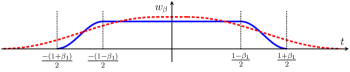
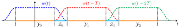
We set in (1) to be a dilated Tukey waveform; in particular, . With this choice of , at any time within the support of , either exactly one or exactly two of the transmitted symbols contribute to . This property facilitates the recovery of phase information from the induced ISI. Accordingly, we define two types of time intervals, to be used in later sections, as follows. For , depends only on whenever . Thus, we define the ISI-free interval as
| (8) |
Similarly, for , depends on both and whenever . Therefore, we define the ISI-present interval as
| (9) |
The ISI-free and ISI-present intervals are shown (for ) in Fig. 3.
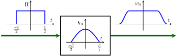
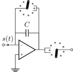
A Tukey waveform may be generated by passing a rectangular pulse
through a linear time-invariant (LTI) filter with impulse response
as shown in Fig. 4. In particular, , where denotes convolution. As will be discussed in Sec. IV, this fact can be exploited for waveform generation at the transmitter.
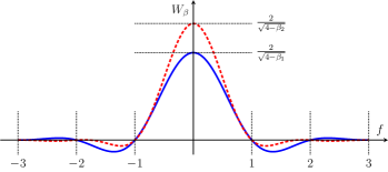
As the waveforms are strictly time-limited, they cannot be bandlimited. The Fourier transform of , denoted as , is
Fig. 5 shows for two different values. Tables I and II give the bandwidth of which contains, respectively, and of the total energy. For these energy percentiles, the out-of-band signal energy is dB and dB less than the in-band energy, respectively. One observes that, although not strictly bandlimited, the bandwidth of is close to for large values of . For example, of the energy is contained within a spectral band of length , i.e., a overhead compared to the minimum bandwidth required for Nyquist signalling. Indeed, the numerical simulations in Sec. III support the use of large values in terms of BER and mutual information.
Note that is not orthogonal to its unit-shift replica, i.e., . This lack of orthogonality must be taken into account when computing the average power of the waveform . Luckily, in the case when the symbols are independent and identically distributed (i.i.d.), Theorem 1 shows that this power is indeed given as the mean squared value of the symbol magnitudes.
Theorem 1.
For a positive integer and , let be i.i.d. zero-mean complex random variables such that and . Furthermore, let
Then,
i.e., the power of converges to in probability.
Proof:
See Appendix. ∎
We remark that finiteness of is a very mild condition which is true for all finite signal constellations and indeed most of the usual distributions over an infinite range.
| bandwidth | overhead | bandwidth | overhead | ||
| bandwidth | overhead | bandwidth | overhead | ||
II-C Photodiode, the Only Source of Noise
The received optical waveform, , is converted to an electrical signal by a photodiode. In our model, the photodiode is the only source of noise. The photodiode has a gain which, for simplicity, is assumed to be unity in this section. However, the actual gain is taken into account in the numerical simulations presented in Sec. III. The output of the photodiode is a real-valued waveform , such that
| (10) |
where and are independent zero-mean white Gaussian random processes with constant two-sided power spectral densities (PSDs) and , respectively. The and terms are known, respectively, as shot noise and thermal noise [8]. It should be mentioned that photodiodes have additional practical deficiencies, such as, e.g., dark current. However, we assume that such effects contribute negligibly compared to the noise terms in (10).
II-D Integrate & Dump
In this section, we discuss the integrate-and-dump unit in Fig 1. As noted in Sec. II-B, at any time within the support of , either exactly one or exactly two of the transmitted symbols contribute to . The integrate-and-dump unit integrates its input waveform over each and interval, producing and , respectively, where and . More precisely,
| (11) |
and
| (12) |
We expand (11) as follows. Let ; then, by using (see Sec. II-A), we get
| (13) |
where
and
Note that , for any , where .
II-E Equivalence Classes
In this section, we describe the first transmitter block in Fig. 1, i.e., choice of class representative. Let denote the function that maps a vector at the input of the signalling block to the corresponding output of the integrate-and-dump block in the absence of noise and loss (i.e., in a back-to-back configuration with ), as shown in Fig. 6. Specifically, if then , where is such that
for , and is such that
for .
We define an equivalence relation on as follows. Two vectors and are said to be square-law identical, denoted , if and only if . If and are not square-law identical, they are said to be square-law distinct, denoted . Since the relation is indeed an equivalence relation, it partitions into disjoint equivalence classes.
Example 1.
Let and . For both of these vectors we have where and . Therefore, , i.e., and are square-law identical. However, for we have where , but ; therefore, .
For any positive integer , let be a set of cardinality , whose elements are complex-valued vectors of length , called symbol blocks, which are square-law distinct. In other words, such that if . Then, the class-representative unit outputs the symbol block if its input is . Note that the entries of symbol blocks are in fact the transmitted symbols, i.e., the set forms a signal constellation in complex dimensions ( real dimensions). Furthermore, note that the spectral efficiency of this communication scheme cannot exceed bit/sec/Hz.

II-F Maximum-Likelihood Block Detection
The last block of Fig. 1 is the detector. In practice, the choice of detection rule and its algorithm will depend on hardware limitations and performance requirements. Through out this paper, maximum-likelihood (ML) block detection is chosen as the detection rule. In other words, if and are the buffered outputs of the integrate-and-dump unit, the detector chooses as the transmitted index if and only if
For any , (13) implies that, given ,
| (15) |
Furthermore, for any , (14) implies that, given and ,
| (16) |
Thus,
| (17) |
where and can be computed from (15) and (16), respectively. Fig. 7 is the factor-graph representation [54] of (17). Note that the variances of and , given in (15) and (16), are functions of the transmitted symbols; therefore, minimum Euclidean-distance detection is not equivalent to ML block detection.

III Numerical Simulation
In this section, the communication scheme proposed in Sec. II is verified by numerical simulations.
III-A The Photodiode
We assume the use of an InGaAs avalanche photodiode (APD), as among different types of APDs, these have high bandwidth. In this case, the two-sided PSD of the thermal noise, , is [8]
where is the Boltzmann constant, is the temperature, and is the external load resistance. Furthermore, for the received optical complex-valued waveform , the shot noise is , where the two-sided PSD of is
where is the unit charge, is the APD gain, is the excess noise factor, and is the responsivity of APD. Table III gives the values for these parameters used in simulations.
| Parameter | Value | |
| Temperature | K | |
| Load Resistance | ||
| APD Gain | ||
| mA/mW | ||
| factor | ||
| Excess Noise Factor |
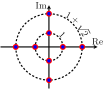
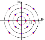
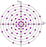
III-B The Transmitted Symbols
The transmitted symbols are chosen from a finite constellation, , five of which are shown in Fig. 8. Indeed, , and since the symbol blocks must be square-law distinct, there is a loss in the maximum achievable rate in the proposed scheme, compared to its coherent-detection counterpart. Table IV provides the number of equivalent classes of each possible size for different values of , and for -ring/-ary phase constellation (see Fig. 8b). For example, for there are equivalence classes, among which have size . As there are possible vectors of length over , the lost rate is bits per symbol. Table IV shows that the larger is , the smaller is the rate loss. However, this reduction in rate loss comes with a higher detection complexity. Specifically, the number of equivalence classes grows exponentially with , which itself increases the complexity of the ML block decoder.
It should be noted that a relatively small suffices to achieve a practical target BER. This is because the transmission scheme is usually the inner-most layer of a larger communication system, which typically also employs an outer error-correcting code.


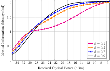
III-C Mutual Information
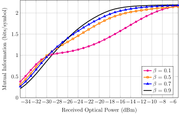
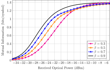
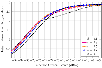
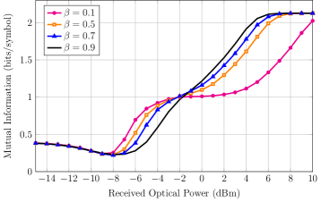
Fig. 9 shows the achievable rate per symbol in different scenarios, plotted against the received optical power (ROP), computed by a Monte Carlo method. To compute the spectral efficiency in bit/sec/Hz one must choose the measure of bandwidth, e.g., in-band energy, in-band energy, etc., that suits the application restrictions. The spectral efficiency can then be computed readily.
In Figs. 9LABEL:sub@fig:24_3–9LABEL:sub@fig:all, the transmitted symbol block is chosen independently and uniformly among all symbol blocks, i.e., class representatives. In Fig. 9LABEL:sub@fig:uniform, instead of square-law distinct symbol blocks, all possible vectors of have been chosen with uniform distribution. As equivalence classes have different cardinalities (see Table IV), a uniform distribution over induces a non-uniform distribution over equivalence-class representatives, giving rise to a huge loss in the achievable rate compared to Figs. 9LABEL:sub@fig:24_3–9LABEL:sub@fig:all. Thus it is important that the transmitted symbol blocks are chosen to be square-law distinct.
As shown in Figs. 9LABEL:sub@fig:24_3–9LABEL:sub@fig:44rate, the value of affects the minimum required power to achieve a target data rate, for a fixed constellation . We find that either outperforms other choices of at close-to-saturation data rates, or the loss is negligible compared to other values of .
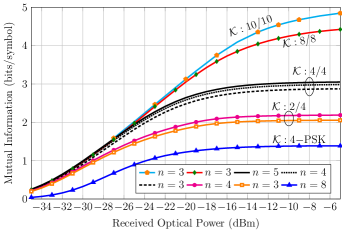
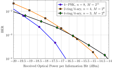
Inspired by [55], Fig. 9LABEL:sub@fig:all shows the mutual information for different constellations and with different values of , all with . This figure can be interpreted in two different ways, as follows. First, by fixing the ROP at a constant value, we can achieve a higher data rate by choosing a larger constellation. For example, at the ROP of dBm and with , a data rate of bit/sym is achievable with the -ring/-ary phase constellation, while a data rate of bit/sym is achievable with the -ring/-ary phase constellation. Secondly, by selecting a larger , a target data rate is achievable at a smaller ROP. For example, the data rate of bit/sym is achievable by the -ring/-ary phase constellation with at an ROP dBm, while by using the -ring/-ary phase constellation, with and a channel code of rate , the same data rate is achievable at the ROP of dBm, i.e., with approximately a dB gain. Note that the number of equivalence classes in the former is , while in the latter it is ; therefore, their ML block-detection complexities are roughly the same.
As discussed earlier in this section, for a fixed constellation , the achievable rate will increase with increasing . This fact can be seen from Fig. 9LABEL:sub@fig:all. For example, while the maximum achievable rate for -ring/-ary phase constellation is bit/sym for , the maximum achievable rate is and bit/sym for and , respectively. If one chooses the in-band energy as the criterion for defining the bandwidth, then the spectral efficiencies for , , and is, respectively, , , and bit/sec/Hz. Note that the maximum rate for this constellation is bit/sec/Hz under coherent detection; therefore, in the last two cases, i.e., and , the rate is within the bounds given in [21, 22]. Furthermore, although the spectral efficiency for is below the rate lower-bound i.e., bit/sec/Hz, the gap is small, i.e., about . By the same bandwidth definition, the maximum spectral efficiency for other constellations in Fig. 9LABEL:sub@fig:all are all within one bit/sec/Hz of coherent detection. However, if one chooses the in-band energy as the criterion for specifying the bandwidth then, except the -PSK constellation, the spectral-efficiency gap with coherent detection is greater than one bit/sec/Hz. For example, the maximum spectral efficiency for -ring/-ary phase constellation with becomes bit/sec/Hz which is smaller than the lower bound, i.e., bit/sec/Hz.
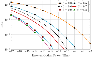
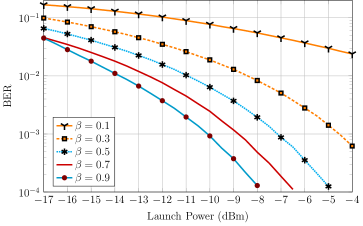
III-D Bit Error Rate
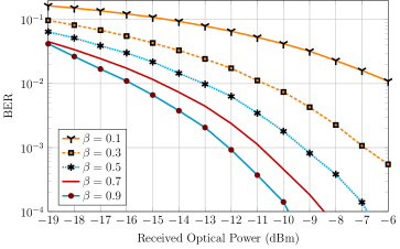
Fig. 10 shows the bit error rate of the proposed scheme in a back-to-back () configuration, for several , , and . In each scenario, is chosen to be an integer power of . For example, while there are equivalence classes for the -ring/-ary phase constellation with , only of them are chosen as the symbol blocks, i.e., members of . The length binary label associated with each of the symbols was chosen randomly, i.e., no particular labelling algorithm, e.g., Gray code, is being used.
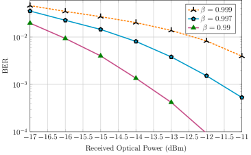
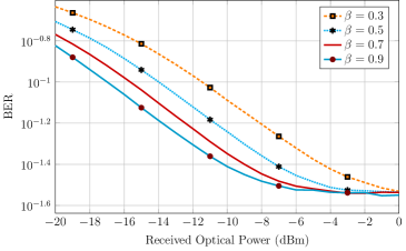
As shown in Fig. 10LABEL:sub@fig:ber_24_small, for the -ring/-ary phase constellation, the BER decreases when increasing from to . It might be perceived from this figure that a larger value of results in a better BER performance; therefore, the best BER performance is achieved for the maximum possible value for , i.e., unity. However, Fig. 10LABEL:sub@fig:ber_24_large refutes this claim. As shown in this figure, for close-to-unity values of , a small increment results in a significant performance loss, in terms of BER. In the extreme case, i.e., , there is no ISI-free sample, and the complex-valued transmitted symbols must be detected from the real-valued ISI-present received samples. Thus, there is a significant performance loss, both in terms of BER and the maximum achievable rate.
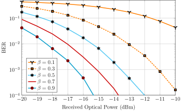
The BER performance under -PSK and -ring/-ary phase constellations are shown in Fig. 10LABEL:sub@fig:ber_4psk and Fig. 10LABEL:sub@fig:ber_44, respectively. In both cases, the performance is improved by increasing from toward .
Despite the fact that has the best BER performance in Fig. 10LABEL:sub@fig:ber_24_small for the -ring/-ary phase constellation, because of the discussed high sensitivity of performance to the value of for , is used to compare the BER of different constellations in Fig. 10LABEL:sub@fig:ber_all. For the purpose of fairness, the horizontal axis is normalized to information rate. Similar to a typical communication over an additive white Gaussian noise (AWGN) channel, for a fixed noise power and at high signal powers, using a larger constellation results in a higher BER; however, at low ROPs, the BER performance is a complicated function of the received power.
The choice of constellation has a big impact on the performance of the proposed scheme. For example, while -QAM (quadrature amplitude modulation) is a typical constellation in communication over AWGN channels, it has very poor performance in the proposed scheme, as shown in Fig. 10LABEL:sub@fig:ber_16qam.
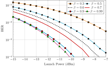
The BER performance for a nonzero fiber length, i.e., , for -ring/-ary and -ring/-ary phase constellations are shown in Figs. 11LABEL:sub@fig:ber_24_ssfm and 11LABEL:sub@fig:ber_44_ssfm, respectively. The split-step Fourier method [56] was used to approximate wave propagation through a km standard single-mode fiber (SSMF) at an operating wavelength of nm. One observes that, by using a -ring/-ary phase constellation with symbol blocks of length and , a BER of is resulted at a dBm launch power. As the power loss of SSMF at this wavelength is about ; a dBm launch power results a dBm ROP. Note that this agrees with Fig. 10LABEL:sub@fig:ber_44, i.e., a BER of resulted from same system parameters at a dBm ROP. At higher launch powers, however, there is a discrepancy between the figures, resulting from uncompensated nonlinear fiber impairments. To achieve a high data rate, one may operate in the low-to-moderate launch-power regime—where fiber nonlinearity is not a critical factor—by choosing high-order constellations. If high detection complexity rules high-order constellations out then one might use low-order constellations and operate at high launch powers by precompensating not only the chromatic dispersion but also the fiber nonlinear impairments at the transmitter. However, such nonlinear precompensation, which might be implemented by a form of digital back-propagation [57], will itself incur significant implementation complexity.
III-E Power
If the transmitted symbols are i.i.d., Theorem 1 guarantees that the average power of the transmitted waveform is equal, in probability, to the variance of those symbols. On the other hand, in Sec. III-C it was noted that uniform selection of symbol blocks from the entire results in a significant loss in achievable rate, and therefore must be avoided. Constraining symbol blocks to be square-law distinct makes the transmitted symbols dependent, and thus Theorem 1 does not apply. However, in the numerical simulations it turned out that the average power of the transmitted waveform is indeed equal to in all cases studied, where is the average power of and where denotes the -norm.
III-F Comparison With Other Schemes
Due to differences in channel models, particularly the idealization of optical fibers, a fair comparison of the proposed scheme with other existing schemes is difficult. For example, while we have assumed that there are no optical amplifiers, and, as a result, no ASE noise in the channel, many papers in the literature use erbium-doped fiber amplifiers, which are primary sources of ASE noise.
Although not exactly fair, to make a comparison, let us assume the proposed scheme is used to transmit data over a span of km of SSMF. The resulting power loss at nm is dB. Factoring in an additional dB loss due, e.g., to connector losses and code operation at some gap to the Shannon limit, let us assume the launch power is dB larger than the received power. In this case, from Fig. 9LABEL:sub@fig:all we see that an information rate of bits per symbol can be achieved with the proposed scheme, either by using the -ring/-ary phase constellation with and a channel code of rate at a launch power of dBm, or by using the -ring/-ary phase constellation with and a channel code of rate at a launch power of dBm. On the other hand, using a Kramers–Kronig receiver, the authors of [26] achieve a data rate of bits per symbol at a launch power of dBm. However, as noted, the channel model of [26] is quite different.
IV Complexity
In this section we discuss the implementation complexity of direct detection under Tukey signalling. Note that the proposed scheme aims to achieve spectral efficiencies close to those of a coherent detector. Therefore—instead of comparing with simple IM/DD schemes whose rates are roughly half the data rate under coherent detection—the complexity of the proposed scheme must be compared with schemes that modulate complex-valued waveforms, e.g., coherent and Kramers–Kronig transceivers.
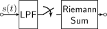
Fig. 12 shows simple examples of analog and digital integrate-and-dump circuits. Other circuit topologies, designed specifically for high baud rate fiber-optic communications, are well investigated [58]. In order to integrate the output of the photodiode over the ISI-free and ISI-present intervals, a clock with a duty cycle of and its inverse is needed. Two analog-to-digital converters (ADCs), each operating at the baud rate, are needed to convert into discrete-time output samples, i.e., ’s and ’s, where and . This number of ADCs is exactly the same as required (per polarization) in coherent detection, as shown in Fig. 13. The spectrum-broadening operations in typical Kramers–Kronig receivers necessitates even higher conversion rates, e.g., six times the baud rate. However, there are some schemes that allow sampling at twice the baud rate, but under some assumptions, e.g., high carrier-to-signal power ratio [59, 60].
Similar to coherent and Kramers–Kronig transceiver schemes, both the in-phase and the quadrature components of the transmitted waveform are modulated. In other words, the electric field itself (and not just the field intensity) is modulated. Therefore, an IQ modulator is needed at the transmitter.
As mentioned in Sec. II-B, ; this property can be exploited in implementing the Tukey waveform at the transmitter. In fact, two zero-order-hold digital-to-analog converters (DACs), one for the in-phase and one for the quadrature components, each operating at the baud rate and of hold-duration , can be used to map the discrete-time transmitted symbols into a train of rectangular waveforms which itself is then filtered by an LTI filter with impulse response , producing . Since has bounded support, the filter has a causal implementation.
Equivalence class representatives for a particular constellation and block length can be pre-computed and stored in a look-up table. Thus there is no operational complexity related to determining the set .
The naive scheme for ML block detection searches over all transmitted blocks to maximize the likelihood score. Therefore, its complexity is , where is the maximum achievable rate with . As mentioned in Sec. III-B, a small suffices to achieve a target BER; thus, the complexity of the ML block detection is a relatively small fixed constant. It may be possible to reduce this complexity, for example, via a trellis-search algorithm, but we leave the investigation of this for future work.


V Discussion
As well stated by Tukey, “the test of a good procedure is how well it works, not how well it is understood” [61]. So far the proposed scheme has been tested only with computer simulations. It would be interesting to investigate its performance in a practical experiment.
Throughout this paper, we have assumed an unamplified optical link and therefore no ASE noise in the system. It would be interesting to investigate the performance of the proposed scheme in the presence of ASE noise.
We have used maximum-likelihood block detection to detect the transmitted symbol block. It would be interesting to investigate other detection strategies. For example, we have assumed that blocks are transmitted without guard time, which means that the last symbol of one block interferes with the first symbol of the next block. While our block detection rule ignores the signal received during these intervals of overlap, a sequence-oriented detection algorithm could potentially exploit them.
Due to chromatic dispersion, polarization mode dispersion, and nonlinear interactions between signals, the optical fiber channel is not memoryless. In our proposed system we have precompensated for chromatic dispersion (a dominant cause of temporal signal broadening, and hence memory); however, we have not studied or compensated for other impairments causing memory. Although these factors may not be significant at short transmission lengths or with relatively low launch power, it would interesting to investigate the transmission regimes where these factors begin to impact performance.
As noted in Sec. II-F, unlike AWGN channels, Euclidean distance is not an appropriate metric for detecting the transmitted symbol block. It would be interesting to derive an appropriate metric for the proposed scheme. In addition to giving an insight on detection, such a metric might simplify the detector’s implementation.
We have used only five different constellations to derive the results in this paper, namely, the -ring/-ary phase, the -ring/-ary phase, and the -PSK constellations, and we have shown that -QAM gives poor performance. Constellation design is thus another interesting research topic that can be addressed in future work. In particular, given a set of performance criteria, it would be interesting to find the “best” constellation that satisfies the conditions. This question is closely related to the question about metrics, since for a given power, the performance of a constellation improves by increasing the minimum distance between its points.
We did not impose any criterion for choosing equivalence-class representatives, i.e., symbol blocks. It would be interesting to see if some particular elements are better than others for use as class representatives.
Although the numerical simulations revealed that the average transmitter power equals in the simulations, it would be interesting to generalize Theorem 1 to allow for dependent symbols. Strengthening the convergence type is another relevant problem.
No doubt many further interesting problems can be posed.
[Proof of Theorem 1] For and , let the ISI-free interval and the ISI-present interval be as given in (8) and (9), respectively. Then,
| (18) |
where , , and
One may see that and .
Let and denote, respectively, the sample average of and random variables, i.e., and . Then, (18) implies that
| (19) |
As ’s are i.i.d. for , the random variables are i.i.d. and have finite variance, where the latter is true as . As a result, by the weak law of large numbers,
| (20) |
Unlike ’s, the random variables, , are dependent. However, the dependency is only between adjacent ’s. In particular, and are dependent, thus, , only if , where and and denotes the covariance. Furthermore, as for all , it implies that . Therefore,
Therefore, , and Chebyshev’s inequality implies that
| (21) |
Furthermore, ; thus,
| (22) |
As a result, (19), (20), (21), and (22) imply that
Acknowledgment
The authors would like to thank Qun Zhang for helpful discussions regarding the split-step Fourier simulation method and an anonymous reviewer whose comments significantly improved the paper.
References
- [1] C. Giacovazzo, Phasing in Crystallography: A Modern Perspective, 1st ed. London, UK: Oxford Univ. Press, 2014.
- [2] B. F. Burke and F. Graham-Smith, An Introduction to Radio Astronomy, 3rd ed. Cambridge, UK: Cambridge Univ. Press, 2009.
- [3] J. Aparici, “A wide dynamic range square–law diode detector (for radioastronomy),” IEEE Trans. Instrum. Meas., vol. 37, no. 3, pp. 429–433, Sep. 1988.
- [4] G. E. Nilsson, T. Tenland, and P. Oberg, “A new instrument for continuous measurement of tissue blood flow by light beating spectroscopy,” IEEE Trans. Biomed. Eng., vol. BME–27, no. 1, pp. 12–19, Jan. 1980.
- [5] F. F. Digham, M. Alouini, and M. K. Simon, “On the energy detection of unknown signals over fading channels,” IEEE Trans. Commun, vol. 55, no. 1, pp. 21–24, Jan. 2007.
- [6] D. R. Hummels, C. Adams, and B. K. Harms, “Filter selection for receivers using square-law detection,” IEEE Trans. Aerosp. Electron. Syst., vol. AES-19, no. 6, pp. 871–883, Nov. 1983.
- [7] B. Xu and M. Brandt-Pearce, “Multiuser detection for square-law receiver under Gaussian channel noise with applications to fiber-optic communications,” IEEE Trans. Inf. Theory, vol. 51, no. 7, pp. 2657–2664, Jul. 2005.
- [8] G. P. Agrawal, Fiber–Optic Communication Systems, 4th ed. NJ, USA: John Wiley & Sons, 2010.
- [9] S. Kumar and M. J. Deen, Fiber Optic Communications: Fundamentals and Applications, 1st ed. UK: John Wiley & Sons, 2014.
- [10] A. Mecozzi and M. Shtaif, “On the capacity of intensity modulated systems using optical amplifiers,” IEEE Photon. Technol. Lett., vol. 13, no. 9, pp. 1029–1031, Sep. 2001.
- [11] M. I. Yousefi and F. R. Kschischang, “The per-sample capacity of zero-dispersion optical fibers,” in 12th Can. Workshop Inf. Theory, Kelowna, BC, Canada, May 2011, pp. 98–101.
- [12] K. S. Turitsyn, S. A. Derevyanko, I. V. Yurkevich, and S. K. Turitsyn, “Information capacity of optical fiber channels with zero average dispersion,” Phys. Rev. Lett., vol. 91, no. 20, p. 203901, Nov. 2003.
- [13] I. Jacobs, “Limits on the power and spectral efficiency of direct detection systems with optical amplifiers,” in 35th Asimolar Conf. Signals Syst. Comput., Pacific Grove, CA, USA, Nov. 2001, pp. 8–12.
- [14] L. Chen, B. Krongold, and J. Evans, “Performance analysis for optical OFDM transmission in short-range IM/DD systems,” J. Lightwave Techn., vol. 30, no. 7, pp. 974–983, Apr. 2012.
- [15] ——, “Theoretical characterization of nonlinear clipping effects in IM/DD optical OFDM systems,” IEEE Trans. Commun., vol. 60, no. 8, pp. 2304–2312, Aug. 2012.
- [16] S. D. Dissanayake and J. Armstrong, “Comparison of ACO-OFDM, DCO-OFDM and ADO-OFDM in IM/DD systems,” J. Lightwave Techn., vol. 31, no. 7, pp. 1063–1072, Apr. 2013.
- [17] B. Karanov et al., “End-to-end deep learning of optical fiber communications,” J. Lightwave Techn., vol. 36, no. 20, pp. 4843–4855, Oct. 2018.
- [18] K. Yonenaga and S. Kuwano, “Dispersion-tolerant optical transmission system using duobinary transmitter and binary receiver,” J. Lightwave Techn., vol. 15, no. 8, pp. 1530–1537, Aug. 1997.
- [19] A. V. T. Cartaxo, “Cross-phase modulation in intensity modulation-direct detection WDM systems with multiple optical amplifiers and dispersion compensators,” J. Lightwave Techn., vol. 17, no. 2, pp. 178–190, Feb. 1999.
- [20] X. Li, R. Mardling, and J. Armstrong, “Channel capacity of IM/DD optical communication systems and of ACO-OFDM,” in IEEE Int. Conf. Commun., Glasgow, UK, Jun. 2007, pp. 2128–2133.
- [21] A. Mecozzi and M. Shtaif, “Information capacity of direct detection optical transmission systems,” J. Lightwave Techn., vol. 36, no. 3, pp. 689–694, Feb. 2018.
- [22] A. Tasbihi and F. R. Kschischang, “On the capacity of waveform channels under square-law detection of time-limited signals,” IEEE Trans. Info. Theory, vol. 66, no. 11, pp. 6682–6687, Nov. 2020.
- [23] A. Mecozzi, C. Antonelli, and M. Shtaif, “Kramers–Kronig coherent receiver,” Optica, vol. 3, no. 11, pp. 1220–1227, 2016.
- [24] Z. Li et al., “SSBI mitigation and the Kramers–Kronig scheme in single-sideband direct-detection transmission with receiver-based electronic dispersion compensation,” J. Lightwave Techn., vol. 35, no. 10, pp. 1887–1893, May 2017.
- [25] X. Chen et al., “218-Gb/s single-wavelength, single-polarization, single-photodiode transmission over 125-km of standard singlemode fiber using Kramers–Kronig detection,” in Proc. Opt. Fiber Commun. Conf. Expo. (OFC), Los Angeles, CA, USA, Mar. 2017, pp. Th5B.6:1–3.
- [26] ——, “Kramers–Kronig receivers for 100-km datacenter interconnects,” J. Lightwave Techn., vol. 36, no. 1, pp. 79–89, Jan. 2018.
- [27] Z. Li et al., “Joint optimisation of resampling rate and carrier-to-signal power ratio in direct-detection Kramers–Kronig receivers,” in Eur. Conf. Opt. Commun. (ECOC), Gothenburg, Sweden, Sep. 2017, pp. 1–3.
- [28] A. Lender, “The duobinary technique for high-speed data transmission,” IEEE Trans. Commun. Electron., vol. 82, no. 2, pp. 214–218, May 1963.
- [29] E. Kretzmer, “Generalization of a techinque for binary data communication,” IEEE Trans. Commun. Technol., vol. 14, no. 1, pp. 67–68, Feb. 1966.
- [30] F. K. Becker, E. R. Kretzmer, and J. R. Sheehan, “A new signal format for efficient data transmisson,” Bell Syst. Tech. J., vol. 45, no. 5, pp. 755–758, May-Jun. 1966.
- [31] J. Smith, “Error control in duobinary data systems by means of null zone detection,” IEEE Trans. Commun. Technol., vol. 16, no. 6, pp. 825–830, Dec. 1968.
- [32] J. Gunn and J. Lombardi, “Error detection for partial-response systems,” IEEE Trans. Commun. Technol., vol. 17, no. 6, pp. 734–737, Dec. 1969.
- [33] H. Kobayashi and D. Tang, “On decoding of correlative level coding systems with ambiguity zone detection,” IEEE Trans. Commun. Technol., vol. 19, no. 4, pp. 467–477, Aug. 1971.
- [34] P. Kabal and S. Pasupathy, “Partial-response signalling,” IEEE Trans. Commun., vol. 23, no. 9, pp. 921–934, Sep. 1975.
- [35] H. Kobayashi and D. Tang, “Application of partial-response channel coding to magnetic recording systems,” IBM J. Res. Dev., vol. 14, no. 4, pp. 368–375, Jul. 1970.
- [36] R. Wood and D. Petersen, “Viterbi detection of class IV partial response on a magnetic recording channel,” IEEE Trans. Commun., vol. COM-34, no. 5, pp. 454–461, May 1986.
- [37] H. Thapar and A. Patel, “A class of partial response systems for increasing storage density in magnetic recording,” IEEE Trans. Magn., vol. 23, no. 5, pp. 3666–3668, Sep. 1987.
- [38] J. E. Mazo, “Faster-than-Nyquist signaling,” Bell Syst. Techn. J., vol. 54, no. 8, pp. 1451–1462, Oct. 1975.
- [39] G. Colavolpe, T. Foggi, A. Modenini, and A. Piemontese, “Faster-than-Nyquist and beyond: How to improve spectral efficiency by accepting interference,” Optics Expr., vol. 19, no. 27, pp. 26 600–26 609, Dec. 2011.
- [40] J. B. Anderson, F. Rusek, and V. Öwall, “Faster-than-Nyquist signaling,” Proc. IEEE, vol. 101, no. 8, pp. 1817–1830, Aug. 2013.
- [41] M. Jana, A. Medra, L. Lampe, and J. Mitra, “Pre-equalized faster-than-Nyquist transmission,” IEEE Trans. Commun, vol. 65, no. 10, pp. 4406–4418, Oct. 2017.
- [42] H. Bülow, F. Buchali, and A. Klekamp, “Electronic dispersion compensation,” J. Lightwave Techn., vol. 26, no. 1, pp. 158–167, Feb. 2008.
- [43] M. M. E. Said, J. Sitch, and M. I. Elmasry, “An electrically pre-equalized 10-Gb/s duobinary transmission system,” J. Lightwave Techn., vol. 23, no. 1, pp. 388–400, Jan. 2005.
- [44] R. I. Killey, P. M. Watts, V. Mikhailov, M. Glick, and P. Bayvel, “Electronic dispersion compensation by signal predistortion using digital processing and a dual-drive Mach-Zehnder modulator,” IEEE Photon. Technol. Lett., vol. 17, no. 3, pp. 714–716, Mar. 2005.
- [45] J. Zhou et al., “Transmission of 100-Gb/s DSB-DMT over 80-km SMF using 10-G class TTA and direct-detection,” in Eur. Conf. Opt. Commun. (ECOC), Dusseldorf, Germany, Sep. 2016, pp. 1–3.
- [46] D. McGhan, C. Laperle, A. Savehenko, C. Li, G. Mak, and M. O’Sullivan, “5120 km RZ-DPSK transmission over G652 fiber at 10 Gb/s with no optical dispersion compensation,” in Proc. Opt. Fiber Commun. Conf. Expo. (OFC), Anaheim, CA, USA, Mar. 2005, pp. PDP27:1–3.
- [47] M. Tomlinson, “New automatic equalizer employing modulo arithmetic,” Electron. Lett., vol. 7, pp. 138–138, Mar. 1971.
- [48] M. Miyakawa and H. Harashima, “A method of code conversion for a digital communication channel with intersymbol interference,” Trans. Inst. Electron. Commun. Eng. Japan, vol. 52-A, pp. 272–273, Jun. 1969.
- [49] W. Yu, D. P. Varodayan, and J. M. Cioffi, “Trellis and convolutional precoding for transmitter-based interference presubtraction,” IEEE Trans. Commun., vol. 53, no. 7, pp. 1220–1230, Jul. 2005.
- [50] E. A. Robinson, “A historical perspective of spectrum estimation,” Proc. IEEE, vol. 70, no. 9, pp. 885–907, Sep. 1982.
- [51] J. W. Tukey, “An introduction to the calculations of numerical spectrum analysis,” in Spectral Analysis of Time Series, B. Harris, Ed. New York, USA: John Wiley & Sons, 1967, pp. 25–46.
- [52] N. Geckinli and D. Yavuz, “Some novel windows and a concise tutorial comparison of window families,” IEEE Trans. Acoust., Speech, Signal Process., vol. 26, no. 6, pp. 501–507, Dec. 1978.
- [53] F. J. Harris, “On the use of windows for harmonic analysis with the discrete Fourier transform,” Proc. IEEE, vol. 66, no. 1, pp. 51–83, Jan. 1978.
- [54] F. R. Kschischang, B. J. Frey, and H. A. Loeliger, “Factor graphs and the sum-product algorithm,” IEEE Trans. Info. Theory, vol. 47, no. 2, pp. 498–519, Feb. 2001.
- [55] G. Ungerboeck, “Channel coding with multilevel/phase signals,” IEEE Trans. Inf. Theory, vol. 28, no. 1, pp. 55–67, Jan. 1982.
- [56] G. P. Agrawal, Nonlinear Fiber Optics, 6th ed. Academic Press, 2019.
- [57] E. Ip and J. M. Kahn, “Compensation of dispersion and nonlinear impairments using digital backpropagation,” J. Lightwave Techn., vol. 26, no. 20, pp. 3416–3425, Oct. 2008.
- [58] A. E. Stevens, “An integrate-and-dump receiver for fiber optic networks,” Ph.D. dissertation, Columbia University, New York, NY, USA, 1995.
- [59] T. Bo and H. Kim, “Kramers–Kronig receiver operable without digital upsampling,” Opt. Express, vol. 26, no. 11, pp. 13 810–13 818, May 2018.
- [60] ——, “Toward practical Kramers–Kronig receiver: Resampling, performance, and implementation,” J. Lightwave Techn., vol. 37, no. 2, pp. 461–469, Jan. 2019.
- [61] D. R. Brillinger, “John W. Tukey: his life and professional contributions,” Ann. Statist., vol. 30, no. 6, pp. 1535–1575, Dec. 2002.