Monopole-Antimonopole Pair Production
in Primordial Magnetic Fields

Takeshi Kobayashi

Kobayashi-Maskawa Institute for the Origin of Particles and the Universe,
Nagoya University, Nagoya 464-8602, Japan

E-mail: takeshi@kmi.nagoya-u.ac.jp

We show that monopoles can be pair produced by cosmological magnetic fields in the early universe. The pair production gives rise to relic monopoles, and at the same time induces a self-screening of the magnetic fields. By studying these effects we derive limits on the monopole mass, and also on the initial amplitude of primordial magnetic fields. Monopoles of GUT scale mass can even be produced if primordial magnetic fields exist at sufficiently high redshifts.

1 Introduction

The hypothesis that magnetic monopoles exist, albeit without any experimental evidence, has long been a subject of intense research. Monopoles would symmetrize Maxwell’s equations, and moreover their existence would be tied to the observed quantization of electric charge through the Dirac quantization condition $eg=2\pi n$, $n\in\mathbb{Z}$ [1]. Besides the possibility that monopoles are elementary particles, they can be realized as topological solitons in spontaneously broken gauge theories as shown by ’t Hooft and Polyakov [2, 3]. The fact that such soliton solutions are contained in any Grand Unified gauge Theory (GUT) in which the electromagnetic U(1) is embedded in a semi-simple gauge group, makes monopoles an inevitable prediction of grand unification.

Despite the strong theoretical support for their existence, monopoles remain elusive in experimental searches. One reason is that their masses are expected to be superheavy. Solitonic monopoles have masses of the order of the symmetry breaking scale, which for GUT monopoles is typically $10^{16}\,\mathrm{GeV}$ and thus is far beyond the reach of terrestrial colliders. This does depend on the model, and much lighter monopoles can also arise, for instance, in theories with several stages of symmetry breaking [4]. However even with a small mass, producing solitonic monopoles at colliders has been argued to be strongly suppressed due to their high degree of compositeness [5, 6]. It is also important to note that the computation of the production cross section of monopoles is a challenging task in itself. This is because the Dirac quantization condition demands $\lvert g\rvert\gg 1$ for $\lvert e\rvert\ll 1$, rendering monopoles strongly coupled and perturbation theory invalid.

On the other hand, a symmetry breaking phase transition in the early universe copiously produces solitonic monopoles with an abundance that would overdominate the present universe, unless the symmetry breaking scale is very low. This was one of the motivations for inflationary cosmology, which dilutes away the monopoles by a period of a rapid cosmological expansion [7, 8, 9, 10]. By solving the monopole problem, however, cosmic inflation also prohibits relic monopoles from a phase transition to be observed.

Another possible venue for monopole production is in strong magnetic fields, from which monopole-antimonopole pairs are non-perturbatively produced. This is the magnetic dual of the Schwinger process [11, 12, 13], and the rate of monopole pair production with arbitrary coupling was computed using an instanton method in [14, 15]. Monopole production from magnetic fields in magnetars (highly magnetized neutron stars with fields up to $B\sim 10^{15}\,\mathrm{G}\sim 10^{-5}\,\mathrm{GeV}^{2}$) and heavy-ion collisions ($B\sim 10^{18}\,\mathrm{G}\sim 10^{-2}\,\mathrm{GeV}^{2}$ at CERN Super Proton Synchrotron) have been studied, by further taking into account finite-temperature effects into the calculations [16, 17, 18, 19] (see [20] for a review). However even in such environments the magnetic fields are not strong enough to produce monopoles with masses much larger than a $\mathrm{GeV}$.

Magnetic fields also exist in the cosmic space on various length scales, with their origin still remaining a mystery. Spiral galaxies are known to host magnetic fields of $B\sim 10^{-5}\,\mathrm{G}$ [21]. Recent gamma ray observations suggest the presence of magnetic fields even in intergalactic voids with strength $B\gtrsim 10^{-15}\,\mathrm{G}$ coherent on Mpc scales or larger [22, 23, 24], giving strong indication that they are remnants of primordial magnetic fields produced in the early universe. Importantly, if (some parts of) the cosmological magnetic fields are actually of primordial origin, then even if their present field strengths are weak, they could have been extremely strong in the early universe.

In this paper we show that (even superheavy) monopole-antimonopole pairs can be produced by primordial magnetic fields, and explore their cosmological implications. A strong enough primordial magnetic field dissipates energy by the monopole pair production, and also by accelerating the monopoles. By evaluating these effects, we obtain consistency conditions for primordial magnetic fields to survive until today to make up the observed magnetic fields, within physical theories that contain either elementary or solitonic monopoles. We also discuss the possibility of primordial magnetic fields producing an observable abundance of monopoles in the universe, or even giving rise to a new kind of monopole problem. Based on these discussions, we derive lower bounds on the monopole mass, under the assumption that the observed cosmological magnetic fields have a primordial origin.

Our discussion regarding the dissipation of primordial magnetic fields is quite distinct from those of the so-called “Parker limit” on the monopole flux, obtained by requiring the survival of galactic magnetic fields [25, 26]. (See also [27] which studied the Parker limit for primordial magnetic fields.) While these works assume a hypothetical abundance of pre-existing monopoles, here the monopoles are produced by the primordial magnetic field itself and thus the monopole abundance is uniquely determined. This enables us to obtain a direct bound on the monopole mass, as a function of the primordial magnetic field strength.

This paper is organized as follows: In Section 2 we compute the number of monopoles produced in primordial magnetic fields. In Section 3 we evaluate the magnetic field dissipation by the monopoles, as well as the monopole relic abundance, and derive limits on the primordial magnetic field strength. In Section 4, the magnetic field limit is translated into limits on the monopole mass, and the energy scale of magnetic field generation. We then conclude in Section 5. In Appendix A we present a general formalism for analyzing the magnetic field dissipation by monopoles, and also analyze effects that are not discussed in the main text. In Appendix B we give the relations between the Hubble rate, cosmic temperature, and redshift during the reheating and radiation-dominated epochs. In Appendix C we give a lower limit on the relic abundance of solitonic monopoles produced at a symmetry breaking phase transition.

Throughout this paper we use Heaviside-Lorentz units, with $c=\hbar=k_{\mathrm{B}}=1$. $M_{\mathrm{Pl}}$ refers to the reduced Planck mass $(8\pi G)^{-1/2}$. Unless explicitly noted, our discussions cover both elementary and solitonic monopoles. The magnetic charge of the monopole is typically large (e.g. $g\approx 21n$ for $e\approx 0.30$), however most of the analyses apply even if $g$ is tiny.

2 Monopole Pair Production in Magnetic Fields

2.1 Vacuum Decay Rate

Analyses of pair production in an external field often invokes a weak coupling, as was also assumed by Schwinger [13], however this does not necessarily apply to monopoles due to the Dirac quantization condition. Using an instanton method, the authors of [14, 15] derived an expression for the vacuum decay rate due to monopole-antimonopole pair production in a static magnetic field as

$$\Gamma=\frac{(gB)^{2}}{(2\pi)^{3}}\exp\left[-\frac{\pi m^{2}}{gB}+\frac{g^{2}}{4}\right],$$ (2.1)

where $B$ is the magnetic field strength, $m$ is the monopole mass, and $g$ is the amplitude of the magnetic coupling (thus $g$ is non-negative hereafter). This result is valid for an arbitrary $g$, as long as the field is sufficiently weak such that

$$\frac{gB}{m^{2}}\lesssim 1,$$ (2.2)

$$\frac{g^{3}B}{m^{2}}\lesssim 4\pi.$$ (2.3)

The second condition suggests that the expression (2.1) is valid while its exponent is negative, and this is stricter than the first condition if $g\gg 1$. It can be understood as the requirement that, in order for the semi-classical instanton techniques used to obtain (2.1) to be valid, the loop radius of the classical instanton solution [14, 15],

$$R=\frac{m}{gB},$$ (2.4)

should be larger than the size of a monopole,

$$r\sim\frac{g^{2}}{4\pi m}.$$ (2.5)

The expression (2.1) can receive corrections also from finite-temperature effects, when the inverse of the temperature of the thermal bath is smaller than the instanton radius, $1/T<R$; such thermal corrections to the monopole production rate have been computed in [16, 18]. Gravitational effects on the monopole production are less studied, but one naively expects that the rate receives corrections when the curvature radius of the spacetime is smaller than $R$; in a Friedmann–Robertson–Walker (FRW) universe, this condition is written as $1/H<R$ where $H$ is the Hubble expansion rate. Moreover, primordial magnetic fields redshift with the expansion of the universe on a time scale of order the Hubble time; this time dependence can also modify the rate if $1/H<R$ (see e.g. [19] for discussions on pair production in spacetime-dependent fields). These corrections would enhance the pair production rate, even enabling the pair production to proceed via sphalerons, if the temperature and/or the Hubble scale are sufficiently high.

We should also note that in (2.1), $m$ and $g$ should be taken to be the renormalized quantities [15]. However we ignore their runnings, which should be good enough for the approximate calculations in this paper.

2.2 Number Density

In order to evaluate the number of monopoles produced from primordial magnetic fields, we identify the decay rate (2.1) with the rate of pair production per unit volume per unit time. Then the number density $n$ of monopole-antimonopole pairs follows

$$\dot{n}=-3Hn+\Gamma,$$ (2.6)

where an overdot denotes a derivative with respect to physical time $t$, and the Hubble rate is $H=\dot{a}/a$ in terms of the scale factor $a$. Considering the magnetic field to be effectively homogeneous, this equation is integrated to yield

$$n(t)=\frac{1}{a(t)^{3}}\int^{t}_{t_{i}}dt^{\prime}\,a(t^{\prime})^{3}\Gamma(t^{\prime}),$$ (2.7)

where $t_{i}$ denotes the time when the magnetic field is switched on. Here, $\Gamma$ depends on time through its dependence on the magnetic field which redshifts with the expansion of the universe. We parameterize the redshifting of the magnetic field strength as

$$B\propto a^{-p},$$ (2.8)

with $p$ being a positive constant of order unity. Without any source, primordial magnetic fields redshift with $p=2$, however different values of $p$ can also be realized in the presence of matter or with stronger electric fields [36]. Here, let us also introduce a dimensionless quantity

$$\epsilon\equiv\frac{gB}{\pi m^{2}},$$ (2.9)

which obeys $\epsilon\ll 1$ when the first weak field condition (2.2) is well satisfied. Since the production rate $\Gamma$ depends exponentially on $B$, it decays very quickly under weak fields on a time scale of $\Delta t_{\Gamma}=\lvert\Gamma/\dot{\Gamma}\rvert\simeq\epsilon/(pH)\ll 1/H$. Hence the integral in (2.7) is dominated by the lower limit, and we obtain an approximate expression for the pair number density valid for $t\gtrsim t_{i}+\Delta t_{\Gamma i}$ as

$$n\sim\frac{(\Delta t_{\Gamma}\,a^{3}\Gamma)_{i}}{a^{3}}=\frac{\epsilon_{i}\Gamma_{i}}{pH_{i}}\left(\frac{a_{i}}{a}\right)^{3},$$ (2.12)

where quantities measured at the initial time $t_{i}$ is denoted by the subscript $i$.

The “initial time” $t_{i}$ which we defined as the moment when the magnetic field switches on and begins to redshift as (2.8), can be understood as the time when the magnetic field generation has concluded. To keep our discussion general we do not specify the concrete mechanism of primordial magnetic field generation, but the time when the generation process completes could for instance be at the end of inflation [37, 38], after inflation when the universe is dominated by an oscillating inflaton [39], or at cosmological phase transitions [40, 41].

3 Effects of Produced Monopoles

As one can read off from the expression (2.1) for $\Gamma$, the exponential suppression factor disappears and monopole production becomes significant as the magnetic field strength approaches the value,

$$B_{\star}=4\pi\frac{m^{2}}{g^{3}}.$$ (3.1)

This is also the field strength which saturates the second weak field condition (2.3). In this section we show that primordial magnetic fields could not have been stronger than $B_{\star}$, by evaluating the backreaction of the monopoles on the magnetic field, and also the monopole relic abundance.

We will mostly consider times long before the electroweak phase transition, therefore the primordial magnetic field and the monopoles are actually those of the hypercharge U(1) gauge field. When these are converted into the magnetic fields and monopoles of the electromagnetic U(1) at the electroweak phase transition, quantities such as the magnetic field strength and magnetic charge will change by a number of order unity that depends on the Weinberg angle, however this will not be important for our discussions.

3.1 Magnetic Field Dissipation by Monopole Production

In terms of the energy density of the magnetic field,

$$\rho_{B}=\frac{B^{2}}{2},$$ (3.2)

the magnetic field scaling (2.8) is rewritten as

$$(\dot{\rho}_{B})_{\mathrm{red}}=-2pH\rho_{B},$$ (3.3)

where we have added a subscript “red” to specify that this contribution to $\dot{\rho}_{B}$ represents the redshifting of the magnetic field due to the cosmic expansion. The time scale of redshifting, $\Delta t_{\mathrm{red}}=\lvert\rho_{B}/(\dot{\rho}_{B})_{\mathrm{red}}\rvert=1/2pH$, is of order the Hubble time.

Additionally, each time the field produces a monopole-antimonopole pair it looses energy corresponding to the rest energy of the pair, $\Delta\mathcal{E}_{B}=-2m$. Thus the energy dissipation due to pair production per unit time and volume is

$$(\dot{\rho}_{B})_{\mathrm{prod}}=-2m\Gamma.$$ (3.4)

This dissipation rate is smaller than the rate of redshifting, i.e. $2m\Gamma<2pH\rho_{B}$, if

$$B<B_{\mathrm{prod}}=\frac{4\pi m^{2}}{g^{3}}\left[1+\frac{4}{g^{2}}\ln\left(\frac{g^{2}}{4\pi^{3}p}\frac{m}{H}\right)\right]^{-1}.$$ (3.5)

A magnetic field stronger than the right hand side would quickly decay through monopole production on a time scale shorter than a Hubble time, until the field falls below $B_{\mathrm{prod}}$. Hence (3.5) gives an upper bound on the primordial magnetic field strength.

The expression for $B_{\mathrm{prod}}$ becomes negative if $(4/g^{2})\ln[(g^{2}/4\pi^{3}p)(m/H)]<-1$. This implies that in such a case the dissipation becomes significant only at very strong fields where the expression (2.1) for $\Gamma$ breaks down. However, the logarithmic term is generically larger than $-1$ if $g\gg 1$: Even in the extreme case where the monopole mass saturates its lower bound $m\gtrsim 1\,\mathrm{GeV}$ derived from heavy-ion collisions [17], and the Hubble scale saturates the upper bound $H\lesssim 10^{14}\,\mathrm{GeV}$ on the inflation scale [42], we get $(4/g^{2})\ln(m/H)\gtrsim-0.5$ as long as $g\gtrsim 16$. Hence by supposing $g\gg 1$ and considering the logarithmic term to be either negligible or positive, we get $B_{\mathrm{prod}}\lesssim B_{\star}$, which guarantees that the weak field conditions (2.2) and (2.3) are satisfied at $B=B_{\mathrm{prod}}$.

One can also check that, under the weak field conditions, the ratio $B/B_{\mathrm{prod}}$ monotonically decreases in time, which indicates that the energy dissipation by the monopoles is more important at earlier times. Hence (3.5) also sets a lower limit on the time of magnetic field generation, as we will see explicitly in Section 4.

3.2 Magnetic Field Dissipation by Monopole Acceleration

After the monopoles are produced, they are accelerated by the magnetic fields and thus further deplete the magnetic field energy. We first evaluate this effect by assuming that the (anti)monopoles move with relativistic velocities $v\simeq 1$ in the (reverse) direction of the magnetic field. Then each (anti)monopole gains kinetic energy of $\Delta\mathcal{E}_{M}=gB\Delta t$, and in turn the magnetic field loses energy per unit time and volume as

$$(\dot{\rho}_{B})_{\mathrm{R}}=-2ngB.$$ (3.6)

Let us for the moment only consider pairs that are produced during an interval $\Delta t_{\Gamma}$ around the time of consideration, and substitute for the pair density (see discussions around (2.12)),

$$n\to\frac{\epsilon\Gamma}{pH}.$$ (3.7)

This amounts to ignoring energy dissipation by the accumulated abundance of monopoles produced in the past, and thus we will obtain a conservative bound on the field strength. Then one finds that the dissipation rate (3.6) due to accelerating relativistic monopoles, is smaller than the rate of redshifting (3.3), i.e. $2ngB<2pH\rho_{B}$, when

$$B<B_{\mathrm{R}}=\frac{\pi m^{2}}{2g}\frac{1}{W(x_{\mathrm{R}})}\quad\mathrm{with}\quad x_{\mathrm{R}}=e^{\frac{g^{2}}{8}}\frac{g}{4\pi p}\frac{m}{H}.$$ (3.8)

Here, $W(x)$ is the Lambert $W$-function which is a solution of $We^{W}=x$; it is non-negative and increasing for $x\geq 0$. $B_{\mathrm{R}}$ also serves as an upper limit on the magnetic field strength, beyond which the field quickly decays by accelerating the monopoles the field itself has produced.

One can obtain an approximate expression for $B_{\mathrm{R}}$ if the first weak field condition (2.2) is well satisfied, i.e. $2gB_{\mathrm{R}}/\pi m^{2}=1/W(x_{\mathrm{R}})\ll 1$. This is equivalent to $x_{\mathrm{R}}\gg 1$, for which we can use the rough approximation $W(x_{\mathrm{R}})\sim\ln x_{\mathrm{R}}$ [43] to obtain

$$B_{\mathrm{R}}\sim\frac{4\pi m^{2}}{g^{3}}\left[1+\frac{8}{g^{2}}\ln\left(\frac{g}{4\pi p}\frac{m}{H}\right)\right]^{-1}.$$ (3.9)

This now takes a form similar to the upper bound (3.5) from pair production, except for the logarithmic factor.

In the above discussions we assumed the monopoles to be relativistic, however one obtains similar results also for non-relativistic monopoles. From the equation of motion of a non-relativistic monopole/antimonopole, $m\ddot{z}=\pm gB$ where $z$ is the direction of the magnetic field, the distance the monopole/antimonopole travels is $\Delta z=\pm(gB/2m)(\Delta t)^{2}$, supposing they are initially at rest. Here we ignored the time dependence of $B$ as well as the effect of the cosmological expansion on the monopole dynamics; this is because we are interested in cases where the magnetic field is dissipated on time scales comparable to or shorter than a Hubble time, and also because we use this computation only while the magnetic field strength changes by an order-unity factor. Thus by accelerating $n$ pairs from zero initial velocity, the magnetic field looses its energy density during $\Delta t$ as

$$-\Delta\rho_{B}=2ngB\lvert\Delta z\rvert=\frac{ng^{2}B^{2}}{m}(\Delta t)^{2}.$$ (3.10)

Equating this with $\rho_{B}$, one obtains the characteristic time scale of magnetic energy dissipation,

$$\Delta t_{\mathrm{NR}}=\frac{1}{g}\sqrt{\frac{m}{2n}}.$$ (3.11)

The condition for this to be longer than the time scale of redshifting $\Delta t_{\mathrm{red}}=1/2pH$ (cf. (3.3)) is obtained by substituting (3.7) for $n$ as

$$B<B_{\mathrm{NR}}=\frac{\pi m^{2}}{3g}\frac{1}{W(x_{\mathrm{NR}})}\quad\mathrm{with}\quad x_{\mathrm{NR}}=e^{\frac{g^{2}}{12}}\frac{g^{2/3}}{6(2\pi)^{1/3}p}\frac{m}{H}.$$ (3.12)

Under the first weak field condition (2.2), this upper limit is approximated by

$$B_{\mathrm{NR}}\sim\frac{4\pi m^{2}}{g^{3}}\left[1+\frac{12}{g^{2}}\ln\left(\frac{g^{2/3}}{6(2\pi)^{1/3}p}\frac{m}{H}\right)\right]^{-1}.$$ (3.13)

Since (3.9) and (3.13) differ only by the logarithmic factor, we conclude that the order of magnitude of the magnetic field limit does not depend on whether the monopoles are relativistic or not.

We have treated the primordial magnetic field as effectively homogeneous, by supposing the coherence length of the field to be larger than the Hubble radius at the time of consideration. In fact, the observationally hinted intergalactic magnetic field typically has a coherence length of Mpc scale or larger [22, 23, 24], which, if it is of primordial origin, re-enters the horizon only at $a_{0}/a\lesssim 10^{6}$. However if the primordial magnetic field had inhomogeneous components with sub-horizon coherence lengths in the early universe, then the monopoles would not always travel in the direction of the magnetic field and thus the energy dissipation via monopole acceleration would be less effective (see [26] for similar discussions for monopoles in galactic magnetic fields).

We also remark that, in the above analyses we only included monopoles produced “on the spot,” and ignored monopoles that have already been produced in the past. Depending on the time evolution of the monopole velocity, the population of monopoles from the past may more effectively deplete the magnetic field energy, in which case the bound on the magnetic field strength becomes even tighter. Discussions on this point, as well as a general formalism for analyzing the magnetic field dissipation by both the production and acceleration of all existing monopoles, are presented in Appendix A.

3.3 Monopole Relic Abundance and Flux

Constraints on the relic density of the produced monopoles yield further limits on primordial magnetic fields. Supposing the monopoles today to be non-relativistic, their relic density is obtained as

$$\rho_{M0}=2mn_{0}\sim\frac{2m\epsilon_{i}\Gamma_{i}}{pH_{i}}\left(\frac{a_{i}}{a_{0}}\right)^{3},$$ (3.14)

where we used (2.12), and the subscript “$0$” denotes values in the present universe. Requiring the density of monopoles not to exceed that of dark matter, i.e. $\rho_{M0}<\rho_{\mathrm{dm}0}\approx 0.3\rho_{\mathrm{crit}0}$ [42], we obtain an upper limit on the initial magnetic field strength (the value when magnetic field generation concludes) as

$$B_{i}<B_{\mathrm{dm}}=\frac{\pi m^{2}}{3g}\frac{1}{W(x_{\mathrm{dm}})}\quad\mathrm{with}\quad x_{\mathrm{dm}}=e^{\frac{g^{2}}{12}}\left(\frac{1}{108\pi p}\frac{m^{5}}{H_{i}\rho_{\mathrm{dm}0}}\right)^{1/3}\frac{a_{i}}{a_{0}}.$$ (3.15)

In order to evaluate $a_{i}/a_{0}$, let us suppose that the generation of the primordial magnetic field concludes at the end of inflation or later, but before matter-radiation equality. We further assume a post-inflation history starting with an epoch dominated by an oscillating inflaton, which eventually decays away and initiates the radiation-dominated epoch. We use the subscript “end” to denote quantities at the end of inflation, “dom” at the time when radiation domination takes over, and “eq” at matter-radiation equality.

The Hubble scale during the post-inflation epochs as a function of the scale factor is given in Appendix B. Using (B.2) and (B.4) to rewrite $a_{i}$ in terms of $H_{i}$, one obtains

$$x_{\mathrm{dm}}\sim e^{\frac{g^{2}}{12}}\frac{1}{p^{1/3}}\left(\frac{m}{10^{9}\,\mathrm{GeV}}\right)^{5/6}\left(\frac{m}{H_{i}}\right)^{5/6}\mathrm{min.}\left\{1,\left(\frac{H_{\mathrm{dom}}}{H_{i}}\right)^{1/6}\right\},$$ (3.16)

where the last factor depends on whether the magnetic field generation completes during radiation domination ($H_{i}<H_{\mathrm{dom}}$), or in an earlier epoch ($H_{i}>H_{\mathrm{dom}}$). Further using the weak field condition, the magnetic field limit is thus approximately written as

$$B_{\mathrm{dm}}\sim\frac{4\pi m^{2}}{g^{3}}\left[1+\frac{12}{g^{2}}\ln\left(\frac{1}{p^{1/3}}\left(\frac{m}{10^{9}\,\mathrm{GeV}}\right)^{5/6}\left(\frac{m}{H_{i}}\right)^{5/6}\mathrm{min.}\left\{1,\left(\frac{H_{\mathrm{dom}}}{H_{i}}\right)^{1/6}\right\}\right)\right]^{-1},$$ (3.17)

which differs from the other bounds only by the logarithmic factor.

A few comments are in order. First, since the monopoles are continuously accelerated by the magnetic fields, they may withstand the Hubble damping and be moving with relativistic velocities in the current universe (cf. Appendix A.2). In such a case, the relic density is larger than (3.14), and the relativistic monopoles serve as extra radiation which is constrained by CMB observations and BBN, yielding a tighter bound on $B_{i}$. Secondly, we assumed that the annihilation of monopoles and antimonopoles does not significantly reduce their abundance. According to the analyses in [44, 45], the annihilation only becomes relevant if the monopole number density is so large as to lead to an overabundance (unless the mass is very light). The discussion may be modified in the presence of cosmological magnetic fields, which pull the monopoles and antimonopoles apart. It will be interesting to study annihilation effects in a magnetic field background.

One can further compute the average flux of monopoles, $F=2n_{0}v_{0}/4\pi$, with $v_{0}$ being the monopole velocity, and compare with various existing bounds [46, 47] including the Parker limit [25, 26, 27]. Depending on the monopole mass, the flux bounds give stronger constraints than $\rho_{M0}<\rho_{\mathrm{dm}0}$. However they do not drastically improve the limit on $B_{i}$, which depends on the bound on the monopole abundance only through the logarithmic factor.

3.4 Remarks on Solitonic Monopoles

For monopoles that are topological solitons of spontaneously broken gauge theories, the discussions above do not apply when the symmetry is unbroken, as then the monopole solution does not exist. Thus strong magnetic fields can exist without producing monopoles while the cosmic temperature and/or the Hubble rate is larger than the symmetry breaking scale, $\sigma<\mathrm{max.}\{T,H\}$. Even with a low temperature and Hubble rate, the magnetic field itself may restore the symmetry if it is stronger than $B_{\star}$ [48, 49, 50]. (The explosive production of monopole-antimonopole pairs at $B\sim B_{\star}$ may be related to this symmetry restoration.) However if the symmetry is unbroken at some time during the post-inflation era, then later at the symmetry breaking phase transition, monopoles are copiously produced and eventually overdominate the universe, unless the symmetry breaking scale is very low. It should also be noted that this monopole problem is particularly severe if the phase transition happens prior to radiation domination (see Appendix C).

Hence, although the magnetic field limits can in principle be evaded by keeping the symmetry unbroken, one has to pay the price of endangering the universe with the monopole problem. Therefore it is safe to assume also for solitonic monopoles that primordial magnetic fields beyond the aforementioned upper limits could not have existed in the post-inflation universe.

We also remark that in a phase of broken symmetry, the magnetic field strength in a radiation-dominated universe is bounded from above by the symmetry breaking scale, thus is typically well below $B_{\star}$. On the other hand, stronger fields can exist in the pre-radiation-dominated era, during which solitonic monopoles can be abundantly produced. We will see this in detail in Section 4.2.

3.5 Summary: A Conservative Bound

In the previous subsections we derived upper limits on the primordial magnetic field amplitude, beyond which the magnetic field self-screens by producing monopole-antimonopole pairs (3.5), or by accelerating the produced monopoles (3.9), (3.13). A cosmological upper limit (3.17) was also derived by the requirement that the magnetic field does not overproduce monopoles in the universe. These limits from self-screening and overproduction are all comparable to or smaller than $B_{\star}$, as one can check by following a discussion similar to that below (3.5).

Potential loopholes to the individual limits were discussed in each subsection, but let us give a few more remarks:

• Corrections to pair production rate. The expression (2.1) for $\Gamma$ used in our analyses can break down at the values of $B$ where self-screening or monopole overproduction takes place, if (a) the weak field conditions are violated, or (b) the cosmic temperature/Hubble scale are sufficiently high to induce finite-temperature/gravitational corrections. We discussed below (3.5) that (a) is unlikely for $g\gg 1$, however there can still be some corrections to $\Gamma$ since $B_{\star}$ only marginally satisfies the second weak field condition (2.3). Regarding (b), note that the radius (2.4) of the classical instanton solution at $B_{\star}$ is $R_{\star}=g^{2}/(4\pi m)$. For solitonic monopoles whose masses are related to the symmetry breaking scale typically via $m\sim g\sigma$, one finds during the symmetry broken phase, i.e. $\sigma>T,H$, that $(4\pi/g)R_{\star}\lesssim 1/T,1/H$. If $g\sim 10$ we get $R_{\star}\lesssim 1/T,1/H$, and hence we can safely use the zero-temperature and flat-space expression (2.1). The corrections, however, may become important if the actual limits such as $B_{\mathrm{prod}}$ are much smaller than $B_{\star}$, or in the late universe when $B$ is small. We also note that this discussion based on the symmetry breaking scale does not directly apply to elementary monopoles. When (2.1) breaks down, pair production tends to take place at a faster rate. Therefore we expect that corrections to $\Gamma$, if any, can only make the upper limits on the primordial magnetic field more stringent.

• Interaction with thermal plasma. We have ignored the interaction of monopoles with the thermal plasma, which can affect our discussions in the following ways: (a) The friction from the plasma may slow down the monopole (see e.g. [51]) and render the magnetic field dissipation via monopole acceleration less efficient. (b) Strong magnetic fields in the pre-radiation-dominated era (such as those generated in the magnetogenesis scenarios of [37, 38, 39]) can give away large energy to the monopoles, which in turn may raise the temperature of the plasma. If such a monopole-mediated reheating were to happen, it would modify the perturbative reheating history we assumed for evaluating the monopole relic density.

• Thermal production. Monopoles can also be thermally produced in the early universe. In particular for solitonic monopoles, according to the analysis in [28], there can be a temperature window below the symmetry breaking scale where an observable monopole abundance is thermally produced. However this analysis assumes entropy conservation after the monopole production, and thus is modified in the pre-radiation-dominated epoch. In any case, the existence of such an additional monopole population would further tighten the magnetic field limits we discussed.

• Effects on magnetic field generation. Our field limits should be applied to primordial magnetic fields after their generation process has completed. This is because during the magnetic field generation, the field can grow faster than it is dissipated by the monopoles, and/or the U(1) gauge theory itself is modified such that the magnetic energy density does not take the form $\rho_{B}=B^{2}/2$ (as is typically the case for Weyl symmetry-breaking magnetogenesis scenarios). If the monopoles are solitonic, modifications of the gauge theory can further affect the monopole solution itself. We also note that the calculation of the monopole relic density is modified if the magnetic field generation completes before the end of inflation. It would be interesting to study how monopoles affect various magnetic field generating mechanisms.

While most of the effects discussed here and in each subsection further tighten our magnetic field limits, some of them may weaken the limits. However we also note that, none of the effects seem capable of evading all limits in one go. Thus we conclude that if either elementary or solitonic monopoles are contained in the physical theory, then the amplitude of primordial magnetic fields in the post-inflation universe is always bounded from above as

$$B\lesssim B_{\star}=4\pi\frac{m^{2}}{g^{3}}.$$ (3.18)

We stress that this is a conservative upper bound, and the magnetic self-screening and/or monopole overproduction can happen with weaker fields.

4 Limits on Monopole Mass and Primordial Magnetic Field

4.1 General Limits

We now discuss the implications of the bound (3.18) for primordial magnetic field generation and monopoles. Below we suppose the magnetic field to redshift consistently as $B\propto a^{-2}$, i.e. (2.8) with $p=2$, after being generated. Then $B_{i}<B_{\star}$ imposes a lower bound on the scale factor (or equivalently an upper bound on the redshift) when the magnetic field generation completes,

$$a_{i}>a_{\star}=a_{0}\left(\frac{B_{0}}{B_{\star}}\right)^{1/2},$$ (4.1)

with the right hand side expressed in terms of the present-day magnetic field strength $B_{0}$. This in turn sets an upper bound on the Hubble scale as $H_{i}<H(a_{\star})$. (We remind the reader that $H_{i}$ is the Hubble scale at the completion of the magnetic field generation; see discussions below (2.12). For instance in inflationary magnetogenesis scenarios where the magnetic fields are excited during the inflation epoch, $H_{i}$ is equal to the Hubble scale at the end of inflation, $H_{\rm{end}}$.)

We assume the magnetic field generation was completed either at the end of inflation, or during the subsequent reheating or radiation-dominated epochs (i.e. $t_{\mathrm{end}}\leq t_{i}<t_{\mathrm{eq}}$), and adopt the usual post-inflation history based on perturbative reheating as described in Section 3.3 or Appendix B. Then calculating $H(a_{\star})$ using (B.2) and (B.4), we obtain an upper limit on $H_{i}$, whose form depends on whether $a_{\star}$ is smaller or larger than the scale factor upon radiation domination $a_{\mathrm{dom}}$,

$$\begin{split}&\quad H_{i}\lesssim H_{\mathrm{dom}}\,\,\mathrm{min.}\left\{\left(\frac{a_{\mathrm{dom}}}{a_{\star}}\right)^{2},\left(\frac{a_{\mathrm{dom}}}{a_{\star}}\right)^{3/2}\right\},\\ \frac{a_{\mathrm{dom}}}{a_{\star}}&\sim\left(\frac{H_{\mathrm{dom}}}{10^{14}\,\mathrm{GeV}}\right)^{-1/2}\left(\frac{B_{0}}{10^{-15}\,\mathrm{G}}\right)^{-1/2}\left(\frac{mg^{-3/2}}{10^{11}\,\mathrm{GeV}}\right).\end{split}$$ (4.2)

The combination $mg^{-3/2}$ derives from (3.18), which traces back to the ratio between the two terms in the exponent of $\Gamma$, cf. (2.1). This upper limit on $H_{i}$ can also be written as a lower limit on the monopole mass,

$$\frac{m}{g^{3/2}}\gtrsim 10^{11}\,\mathrm{GeV}\left(\frac{B_{0}}{10^{-15}\,\mathrm{G}}\right)^{1/2}\left(\frac{H_{i}}{10^{14}\,\mathrm{GeV}}\right)^{1/2}\mathrm{max.}\left\{1,\left(\frac{H_{i}}{H_{\mathrm{dom}}}\right)^{1/6}\right\}.$$ (4.3)

Thus we have obtained a consistency bound on monopoles ($m$, $g$) and primordial magnetic fields ($B_{0}$, $H_{i}$), for a given post-inflation history characterized by $H_{\mathrm{dom}}$.

The temperature at the onset of radiation domination, $T_{\mathrm{dom}}$, which is often referred to as the reheat temperature, is related to $H_{\mathrm{dom}}$ via (B.4). It is required to lie within the range $10^{-3}\,\mathrm{GeV}\lesssim T_{\mathrm{dom}}\lesssim 10^{16}\,\mathrm{GeV}$, where the lower bound comes from BBN and the upper bound is from the observational limit on the energy scale of inflation [42]. The reference value for the present-day magnetic field in the above expressions is taken from the claimed lower limit $B_{0}\gtrsim 10^{-15}\,\mathrm{G}$ on intergalactic magnetic fields from gamma ray observations [22, 23, 24]. (If the coherence length $\lambda$ of the magnetic field is much smaller than a Mpc, the lower limit improves as $\lambda^{-1/2}$.) We also remark that a primordial magnetic field, if homogeneous, is bounded from above as $B_{0}\lesssim 10^{-9}\,\mathrm{G}$ from CMB anisotropies [52], although it has also been claimed that this limit is relaxed in the presence of free-streaming particles like neutrinos [53].

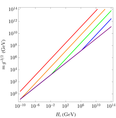
Figure 1: Lower limit on $mg^{-3/2}$ ($m$: monopole mass, $g$: magnetic charge) as a function of the Hubble scale $H_{i}$ when primordial magnetic fields are initially generated. The present-day magnetic field strength is taken as $B_{0}=10^{-15}\,\mathrm{G}$. The cosmic temperature when radiation domination takes over is varied as $T_{\mathrm{dom}}=10^{16}\,\mathrm{GeV}$ (purple), $10^{12}\,\mathrm{GeV}$ (blue), $10^{8}\,\mathrm{GeV}$ (green), $10^{4}\,\mathrm{GeV}$ (orange), and $1\,\mathrm{GeV}$ (red).

In Figure 1 we plot the lower limit (4.3) on $mg^{-3/2}$ as a function of $H_{i}$ (or equivalently the upper limit (4.2) on $H_{i}$ in terms of $mg^{-3/2}$). Here, the present-day magnetic field strength is fixed to the minimum value for intergalactic magnetic fields, $B_{0}=10^{-15}\,\mathrm{G}$, and the limits are shown for $T_{\mathrm{dom}}=10^{16}\,\mathrm{GeV}$ (purple), $10^{12}\,\mathrm{GeV}$ (blue), $10^{8}\,\mathrm{GeV}$ (green), $10^{4}\,\mathrm{GeV}$ (orange), and $1\,\mathrm{GeV}$ (red). The colored lines in the plot overlap at $H_{i}\leq H_{\mathrm{dom}}$, where the limit becomes independent of $H_{\mathrm{dom}}$; in other words, the bend in the line is at $H_{i}=H_{\mathrm{dom}}$. As one goes towards larger $H_{i}$ (magnetic field generation at earlier times), a stronger initial magnetic field is required to survive the more substantial redshifting, and therefore the lower limit on $mg^{-3/2}$ becomes more stringent. The same is true for lower $T_{\mathrm{dom}}$ when $H_{i}>H_{\mathrm{dom}}$, which can be understood from the fact that the universe expands more rapidly during an inflaton domination than radiation domination.

In the parameter regions slightly above the colored lines, an observable abundance of monopoles, but not so large as to overdominate the universe, could be produced. One sees that even monopoles of GUT scale mass ($m=10^{16}\,\mathrm{GeV}$ with, say, $g=10$ gives $mg^{-3/2}\sim 10^{14}\,\mathrm{GeV}$) are produced if magnetic field generation takes place at sufficiently high energy scales.

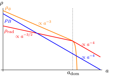
Figure 2: Schematic of the evolution of energy densities in the reheating and radiation-dominated epochs as functions of the scale factor, in log-log scale. Shown are the energy densities of an oscillating inflaton (orange), radiation (red), and primordial magnetic fields (blue). Here the magnetic field energy density is extrapolated back to the left edge of the plot (which corresponds to some time during reheating), but there is actually a cutoff corresponding to the time when the magnetic fields are generated. See the text for details.

Our bound also sets an upper limit on the scale $H_{i}$ of magnetic field generation, for a given value of $mg^{-3/2}$. Let us also comment on other bounds on $H_{i}$. Firstly, as we are assuming the magnetic field generation to conclude between the end of inflation and matter-radiation equality, the Hubble scale should lie within the range $10^{-37}\,\mathrm{GeV}\lesssim H_{i}\lesssim 10^{14}\,\mathrm{GeV}$, where the upper bound is the observational limit on the inflation scale. Secondly, we have assumed that the magnetic field only gives a subdominant contribution to the total energy density of the universe. The time evolution of the energy densities in the post-inflation era is illustrated in Figure 2. Here the orange line denotes the energy density of an oscillating inflaton $\rho_{\phi}$, and the red line denotes the radiation energy density $\rho_{\mathrm{rad}}$ which is created by the decay of the inflaton. Since the generation of primordial magnetic fields and reheating are in general different processes, we discuss the energy density of the magnetic field $\rho_{B}$ separately from $\rho_{\mathrm{rad}}$, and denote it by the blue line in the figure. By extrapolating the magnetic energy density back in time as $\rho_{B}\propto a^{-4}$, it can overtake $\rho_{\phi}$ in the reheating epoch and dominate the universe, which would signal that the cosmological expansion history was once significantly affected by the magnetic field. However the scaling $\rho_{B}\propto a^{-4}$ is actually cut off at the time $t_{i}$, and we constrain this by requiring that the magnetic energy density never dominated the universe. By using (B.2) and (B.4), the magnetic energy fraction at $t_{i}$ is written as

$$\frac{\rho_{Bi}}{3M_{\mathrm{Pl}}^{2}H_{i}^{2}}\sim 10^{-19}\left(\frac{B_{0}}{10^{-15}\,\mathrm{G}}\right)^{2}\mathrm{max.}\left\{1,\left(\frac{H_{i}}{H_{\mathrm{dom}}}\right)^{2/3}\right\},$$ (4.4)

which is smaller than unity if $H_{i}\leq H_{\mathrm{dom}}$ and $B_{0}\lesssim 10^{-6}\,\mathrm{G}$. However in cases with $H_{i}>H_{\mathrm{dom}}$, then $\rho_{Bi}<3M_{\mathrm{Pl}}^{2}H_{i}^{2}$ requires

$$H_{i}\lesssim 10^{10}\,\mathrm{GeV}\left(\frac{B_{0}}{10^{-15}\,\mathrm{G}}\right)^{-3}\left(\frac{T_{\mathrm{dom}}}{1\,\mathrm{GeV}}\right)^{2},$$ (4.5)

where we have rewritten $H_{\mathrm{dom}}$ in terms of $T_{\mathrm{dom}}$. This condition is satisfied on the limits displayed in the plot; e.g., on the red line ($T_{\mathrm{dom}}=1\,\mathrm{GeV}$), the condition is violated at $H_{i}\gtrsim 10^{10}\,\mathrm{GeV}$ which is around the upper edge and beyond. Both upper limits on $H_{i}$, (4.2) and (4.5), are tightened by a larger value of $B_{0}$; we will see this explicitly below.

4.2 Further Limits for Solitonic Monopoles

For solitonic monopoles of spontaneously broken gauge theories, the mass limit (4.3) can be evaded by keeping the symmetry unbroken when the magnetic field is generated. However in such a case the monopoles produced later at the symmetry breaking phase transition would induce a monopole problem, unless the symmetry breaking scale is very low (see also discussions in Section 3.4 and Appendix C). Thus we can combine the requirement to avoid a post-inflation symmetry breaking with the mass limit, and give further constraints for solitonic monopoles.

In the following, for concreteness, we study the vanilla ’t Hooft–Polyakov monopole of an SO(3) gauge theory spontaneously broken to U(1) [2, 3]. In this case the monopole mass is related to the vacuum expectation value of a triplet Higgs field $\sigma$, which we also refer to as the symmetry breaking scale, via $m\sim g\sigma$ (the exact value depends also on the Higgs self-coupling [29]). The magnetic charge is $g=4\pi/e$ in terms of the gauge coupling $e$.

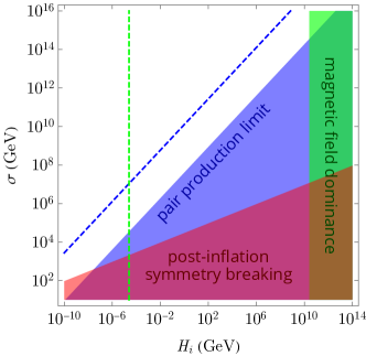
(a) $T_{\mathrm{dom}}=1\,\mathrm{GeV}$

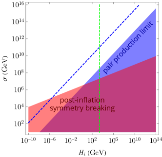
(b) $T_{\mathrm{dom}}=10^{4}\,\mathrm{GeV}$

(c) $T_{\mathrm{dom}}=10^{8}\,\mathrm{GeV}$

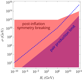
(d) $T_{\mathrm{dom}}=10^{12}\,\mathrm{GeV}$

Figure 3: Parameter space of ’t Hooft–Polyakov monopoles in the plane of the Hubble scale $H_{i}$ when primordial magnetic fields are initially generated, and the symmetry breaking scale $\sigma$. The magnetic charge is fixed to $g=10$, and the present-day magnetic field strength to $B_{0}=10^{-15}\,\mathrm{G}$. The cosmic temperature $T_{\mathrm{dom}}$ when radiation domination begins is varied in the four plots. The blue region violates the monopole mass limit (4.3) obtained by the analyses of pair production in primordial magnetic fields. The green region is excluded by magnetic field dominance in the early universe. In the red region the symmetry breaking phase transition happens after inflation. For a stronger magnetic field $B_{0}=10^{-10}\,\mathrm{G}$, the left edges of the blue and green regions shift to the positions depicted by the dashed lines.

To avoid a symmetry breaking after inflation, the symmetry breaking scale should be high enough to satisfy $\sigma>\mathrm{max.}\{T,H\}$ throughout the post-inflation universe. During radiation domination, this implies $\rho_{B}\sim B^{2}\lesssim\rho_{\mathrm{rad}}\sim T^{4}\lesssim\sigma^{4}$ (here we neglect numerical coefficients). Hence with $m\sim g\sigma$, we get $B\lesssim gB_{\star}$. Thus one sees that if, say, $g=\mathcal{O}(10)$, then unless the inequalities are close to being saturated, the magnetic field in the symmetry broken phase is well below the threshold value $B_{\star}$ for significant monopole production (although there can still be non-negligible effects below $B_{\star}$ as discussed in the previous sections). However this is no longer the case in the epoch prior to radiation domination, where $\rho_{B}$ can be larger than $\rho_{\mathrm{rad}}$, while being smaller than the dominant inflaton energy density (cf. Figure 2). This kind of situation can arise, for instance, in magnetic field generating mechanisms that invoke a violation of the Weyl invariance of the Yang–Mills action (see e.g. [37, 38]); these take place only in a cold universe such as during inflation, since otherwise electrically charged particles in the thermal plasma freeze in the magnetic flux. While such mechanisms are in operation, the energy density of the magnetic field is typically much larger than that of the radiation component.

In Figure 3 we show the parameter space of ’t Hooft–Polyakov monopoles in the $H_{i}$-$\sigma$ plane, where we took $m=g\sigma$, $g=10$, and $B_{0}=10^{-15}\,\mathrm{G}$. $T_{\mathrm{dom}}$ is varied in the four plots as $1\,\mathrm{GeV}$, $10^{4}\,\mathrm{GeV}$, $10^{8}\,\mathrm{GeV}$, and $10^{12}\,\mathrm{GeV}$. The blue region is excluded by the lower limit (4.3) on the monopole mass, and corresponds to that shown in Figure 1. The green region violates the magnetic field energy bound (4.5), which is seen only in the plot for $T_{\mathrm{dom}}=1\,\mathrm{GeV}$, since for $T_{\mathrm{dom}}\gtrsim 10^{2}\,\mathrm{GeV}$ the upper limit on $H_{i}$ from this bound exceeds the highest possible inflation scale. The red region shows where $\sigma<\mathrm{max.}\{T_{i},T_{\mathrm{dom}}\}$, indicating that the symmetry breaking takes place after inflation and thus possibly gives rise to a monopole problem. Here, $T_{i}$ is given in terms of $H_{i}$ through (B.2) and (B.3). We do not show where $\sigma<\mathrm{max.}\{H_{i},H_{\mathrm{dom}}\}$ since it only gives constraints weaker than the other conditions in the displayed parameter regions.

As we have already discussed, the requirement of $\sigma>\mathrm{max.}\{T_{i},T_{\mathrm{dom}}\}$ gives a stronger constraint than the mass limit (4.3) during radiation domination ($H_{i}<H_{\mathrm{dom}}$), and serves as the dominant constraint in the entire displayed space in the plot for $T_{\mathrm{dom}}=10^{12}\,\mathrm{GeV}$. For the other plots with lower $T_{\mathrm{dom}}$, the mass limit dominates at $H_{i}\gg H_{\mathrm{dom}}$, i.e., if the primordial magnetic field is generated long before radiation domination. The combination of $\sigma>\mathrm{max.}\{T_{i},T_{\mathrm{dom}}\}$ and the mass limit (4.3) put severe constraints on symmetry breaking at intermediate and low scales. For instance, the necessary condition for $\sigma=10^{8}\,\mathrm{GeV}$ to evade the two constraints is that $T_{\mathrm{dom}}<10^{8}\,\mathrm{GeV}$ and $H_{i}\lesssim 10^{3}\,\mathrm{GeV}$ are both satisfied.

The condition $\sigma>\mathrm{max.}\{T_{i},T_{\mathrm{dom}}\}$ is independent of $B_{0}$, while the limits (4.3) and (4.5) become stronger for a larger $B_{0}$. In the plots we also show (4.3) and (4.5) for $B_{0}=10^{-10}\,\mathrm{G}$, by the blue and green dashed lines, respectively. With this larger $B_{0}$, the monopole mass limit is tightened by about two orders of magnitude, and overtakes the constraint from $\sigma>\mathrm{max.}\{T_{i},T_{\mathrm{dom}}\}$ in a wider parameter range. The magnetic energy bound is also tightened, and is seen to constrain the high-$H_{i}$ regions in the plots with $T_{\mathrm{dom}}$ up to $10^{8}\,\mathrm{GeV}$.

Note that, to keep the discussion general, we have not specified the inflation scale. We focused on the time $t_{i}$ at the end of magnetic field generation which may coincide with the end of inflation, but can also be at some later time. Accordingly, we only imposed $\sigma>\mathrm{max.}\{T_{i},H_{i},T_{\mathrm{dom}},H_{\mathrm{dom}}\}$, i.e. the symmetry to be broken by the time when magnetic field generation completes or radiation domination begins, whichever happens earlier, instead of imposing $\sigma>\mathrm{max.}\{T,H\}$ since the end of inflation. The actual lower bound on $\sigma$ for evading a post-inflation symmetry breaking would be tighter than shown in the figure, if radiation domination and magnetic field generation take place long after the end of inflation.

5 Conclusions

We showed that the process of pair production in primordial magnetic fields provides an excellent opportunity to confront magnetic monopoles with astrophysical observations. We analyzed two major consequences of the monopole pair production: (i) Primordial magnetic fields dissipate energy by producing the monopole pairs and subsequently accelerating them. This fact that the field self-screens yields a consistency condition for primordial magnetic fields to survive until today and explain the observed magnetic fields. (ii) The pair produced monopoles can give rise to a new type of monopole problem, which gives a cosmological bound on monopoles and primordial magnetic fields. After evaluating the constraints from each effect, we used the most conservative bound on the primordial magnetic field amplitude (3.18) to derive a lower limit on the monopole mass (4.3):

$$m\gtrsim 10^{13}\,\mathrm{GeV}\left(\frac{g}{20}\right)^{3/2}\left(\frac{B_{0}}{10^{-15}\,\mathrm{G}}\right)^{1/2}\left(\frac{H_{i}}{10^{14}\,\mathrm{GeV}}\right)^{1/2}\mathrm{max.}\left\{1,\left(\frac{H_{i}}{H_{\mathrm{dom}}}\right)^{1/6}\right\}.$$ (5.1)

Here $g$ is the magnetic charge of the monopole, $B_{0}$ is the present-day magnetic field strength, $H_{i}$ is the Hubble scale when the primordial magnetic field is initially generated, and $H_{\mathrm{dom}}$ is the Hubble scale when radiation domination begins. This limit also serves as an upper bound on the scale of magnetic field generation. A primordial magnetic field that seeds the observationally suggested intergalactic magnetic fields of $B_{0}\gtrsim 10^{15}\,\mathrm{GeV}$, imposes constraints on monopoles for a wide mass range (Figure 1). This also sets a constraint on grand unified theories, which is particularly severe for models with intermediate and low scale symmetry breaking. Moreover, we showed that even superheavy monopoles of $m\sim 10^{16}\,\mathrm{GeV}$ can be abundantly produced if primordial magnetic fields exist at sufficiently high redshifts.

It is also important to know the exact abundance of monopoles produced in primordial magnetic fields, in order to make concrete predictions for monopole search experiments. Because the pair production rate depends exponentially on the magnetic field, the threshold field strengths for magnetic self-screening and monopole overabundance are typically of the same order. Moreover, this threshold value may only marginally satisfy the weak field condition invoked in the instanton calculation of the pair production rate. Therefore a precise evaluation of the monopole abundance would require solving the full system including the backreaction from the monopoles on the magnetic field, with possible corrections to the pair production rate for marginally weak fields. Additional effects that deserve careful studies are listed in Section 3.5. Taking into account all of them can be non-trivial, however there may be fortunate circumstances where some effects decouple from the rest to simplify the analysis. Alternatively, if some effects can be argued to work only in a certain direction, such as to always enhance the pair production, then one can ignore those effects to derive conservative limits, which is the strategy adopted in this paper. Despite being conservative, our constraint should be useful since it applies to monopoles with a wide mass range, including superheavy ones that are practically impossible to probe in colliders.

Magnetic field generation in the early universe can be accompanied by a simultaneous generation of electric fields, which are considered to eventually short out during the reheating process. It would be interesting to study monopole production in primordial magnetic and electric fields before the latter vanish (see e.g. [54, 55] for studies of Schwinger pair production in electric and magnetic fields). We also note that our analyses can be extended to the production of dyons [56] from primordial electromagnetic fields. Finally we note that the pair production in primordial fields works equally effective for monopoles and magnetic fields of hidden U(1) gauge fields, therefore it can provide a new production mechanism for hidden monopole dark matter [57].

Ultimately, one wishes to probe theories of monopoles and quantum vacuum instability via astrophysical measurements of cosmological magnetic fields, and in turn, to reveal the origin of cosmological magnetic fields by studying monopole pair production. This paper serves as a first step towards this goal.

Appendix A General Discussion of Magnetic Field Dissipation by Monopoles

We present a general discussion on the dissipation of cosmological magnetic fields by monopoles.

A.1 General Formalism

The physical energy density of a spatially homogeneous magnetic field in an FRW background universe obeys

$$d\left[\rho_{B}(t)a(t)^{3}\right]=-P_{B}(t)\,d\left[a(t)^{3}\right]-2m\Gamma(t)a(t)^{3}dt-2gB(t)dt\int^{t}_{-\infty}dt^{\prime}\,a(t^{\prime})^{3}\Gamma(t^{\prime})v(t^{\prime},t),$$ (A.1)

where $P_{B}$ is the pressure of the magnetic fluid, and $\Gamma$ is the rate of monopole-antimonopole pair production by the magnetic field. The second term in the right hand side denotes the magnetic field energy being depleted by $2m$ for the production of each pair, assuming the pairs to be produced at rest (this term corresponds to (3.4)). The third term represents the energy loss by accelerating the population of pairs produced from the infinite past to time $t$, where it should be noted that $a(t^{\prime})^{3}\Gamma(t^{\prime})dt^{\prime}$ gives the comoving number density of pairs produced between $t^{\prime}$ and $t^{\prime}+dt^{\prime}$. Moreover, we used $v(t^{\prime},t)$ to denote the velocity of monopoles produced at $t^{\prime}$, measured at $t$ ($\geq t^{\prime}$), in the direction of the magnetic field (antimonopoles are taken to have charge $-g$ and velocity $-v(t^{\prime},t)$). We have ignored monopole-antimonopole annihilation.

Using $\rho_{B}=B^{2}/2$, and supposing a barotropic equation of state $P_{B}/\rho_{B}=(2p/3)-1$ for the magnetic fluid, which amounts to supposing $B\propto a^{-p}$ in the absence of monopole production, then (A.1) is rewritten as

$$\frac{\dot{\rho}_{B}}{\rho_{B}}=-\Pi_{\mathrm{red}}-\Pi_{\mathrm{prod}}-\Pi_{\mathrm{acc}},$$ (A.2)

with the damping rates due to redshifting, monopole production, and monopole acceleration:

$$\Pi_{\mathrm{red}}(t)=2pH(t),\quad\Pi_{\mathrm{prod}}(t)=\frac{4m\Gamma(t)}{B(t)^{2}},\quad\Pi_{\mathrm{acc}}(t)=\frac{4g}{a(t)^{3}B(t)}\int^{t}_{-\infty}dt^{\prime}\,a(t^{\prime})^{3}\Gamma(t^{\prime})v(t^{\prime},t).$$ (A.3)

The depletion of the magnetic field energy can be studied by solving this equation, combined with the expression (A.6) for $v(t^{\prime},t)$ given below.

A.2 Monopole Velocity

The motion of a monopole with magnetic charge $g$ in a homogeneous magnetic field and an FRW background spacetime is described by the equation of motion,

$$\frac{m}{a}\frac{d}{dt}\left(a\gamma v\right)=gB,\quad\gamma=\frac{1}{\sqrt{1-v^{2}}},$$ (A.4)

where $v$ is the velocity in the direction of the magnetic field, and we neglected motion perpendicular to the magnetic field. This is integrated as

$$\gamma(t^{\prime},t)\,v(t^{\prime},t)=\frac{g}{ma(t)}\int_{t^{\prime}}^{t}dt^{\prime\prime}\,a(t^{\prime\prime})B(t^{\prime\prime}),$$ (A.5)

or equivalently,

$$v(t^{\prime},t)=\frac{\frac{g}{ma(t)}\int_{t^{\prime}}^{t}dt^{\prime\prime}\,a(t^{\prime\prime})B(t^{\prime\prime})}{\sqrt{1+\left[\frac{g}{ma(t)}\int_{t^{\prime}}^{t}dt^{\prime\prime}\,a(t^{\prime\prime})B(t^{\prime\prime})\right]^{2}}}.$$ (A.6)

Here $t$ is the time when the velocity is measured, and $t^{\prime}$ is when the monopole was initially produced at rest.

For example, if the magnetic field scales as $B\propto a^{-p}$, and the Hubble rate as $H\propto a^{-3(1+w)/2}$ with a constant equation of state $w$, the integral can be directly performed as

$$\gamma v=\frac{1}{1-\nu}\frac{gB^{\prime}}{mH^{\prime}}\left[\left(\frac{a^{\prime}}{a}\right)^{\nu}-\left(\frac{a^{\prime}}{a}\right)\right],\quad\nu=p-\frac{3(1+w)}{2},$$ (A.7)

where $a=a(t)$, $a^{\prime}=a(t^{\prime})$, etc. The behavior of $\gamma v$ in the asymptotic future is as follows: If $\nu>0$, it decays in time as either $\gamma v\propto a^{-1}$ ($\nu>1$), $\gamma v\propto a^{-1}\ln a$ ($\nu=1$), or $\gamma v\propto a^{-\nu}$ ($0<\nu<1$). If $\nu<0$, it grows as $\gamma v\propto a^{\lvert\nu\rvert}$. If $\nu=0$, i.e. the equation of state of the universe equals that of the magnetic fluid, then it asymptotes to a constant value $\gamma v\rightarrow gB^{\prime}/mH^{\prime}$.

A.3 Case Studies of Dissipation by Monopole Acceleration

Let us evaluate the dissipation rate by monopole acceleration, $\Pi_{\mathrm{acc}}$, under the simplifying assumption that the magnetic field is suddenly switched on at time $t_{i}$, then subsequently redshifts as $B\propto a^{-p}$ with a positive $p$ of order unity (while the dissipation by monopoles is negligible). Then with $\Gamma$ of the form (2.1), the integral for $\Pi_{\mathrm{acc}}$ is dominated by the contribution from $t_{i}\leq t^{\prime}\lesssim t_{i}+\Delta t_{\Gamma i}$ where $\Delta t_{\Gamma i}=\epsilon_{i}/pH_{i}$ ($\ll 1/H_{i}$, see discussions below (2.9)). Ignoring the variation of $a^{3}\Gamma$ during this period (which implicitly assumes $\Delta t_{\Gamma i}<\Pi_{\mathrm{prod}\,i}^{-1},\Pi_{\mathrm{acc}\,i}^{-1}$), we get

$$\Pi_{\mathrm{acc}}(t)\simeq\frac{4g\Gamma_{i}}{B(t)}\left(\frac{a_{i}}{a(t)}\right)^{3}\int^{t_{i}+\Delta t_{\Gamma i}}_{t_{i}}dt^{\prime}v(t^{\prime},t),$$ (A.8)

for $t\geq t_{i}+\Delta t_{\Gamma i}$. For a further evaluation, we consider some limiting cases below.

A.3.1 Monopoles Produced on the Spot

We start by considering the times $\Delta t_{\Gamma i}\ll t-t_{i}\lesssim 1/H_{i}$, which are within a Hubble time after the magnetic field is switched on. During this period the expansion of the universe can be ignored. Further supposing $B$ to be nearly constant (which amounts to ignoring the backreaction from the monopoles), then (A.8) is approximated as

$$\Pi_{\mathrm{acc}}(t)\simeq\frac{4g\Gamma_{i}}{B_{i}}\int^{t_{i}+\Delta t_{\Gamma i}}_{t_{i}}dt^{\prime}v(t^{\prime},t).$$ (A.9)

Likewise, the monopole velocity (A.6) in the integral is approximated as

$$v(t^{\prime},t)\simeq\frac{\frac{gB_{i}}{m}(t-t^{\prime})}{\sqrt{1+\left[\frac{gB_{i}}{m}(t-t^{\prime})\right]^{2}}}.$$ (A.10)

If the initial magnetic field is sufficiently strong such that the monopoles are relativistic at the time of consideration, i.e. $(gB_{i}/m)(t-t_{i})\gg 1$, then $\int dt^{\prime}v\simeq\Delta t_{\Gamma i}$ and we obtain

$$\Pi_{\mathrm{acc}}\simeq\frac{4g^{2}\Gamma_{i}}{\pi pm^{2}H_{i}}.$$ (A.11)

This matches with the dissipation rate $\lvert(\dot{\rho}_{B})_{\mathrm{R}}/\rho_{B}\rvert$ of (3.6) with the substitution of (3.7) and $t=t_{i}$.

On the other hand for non-relativistic monopoles, i.e. $(gB_{i}/m)(t-t_{i})\ll 1$, then $\int dt^{\prime}v\simeq(gB_{i}/m)\Delta t_{\Gamma i}(t-t_{i})$ and we get

$$\Pi_{\mathrm{acc}}\simeq\frac{4g^{3}B_{i}\Gamma_{i}}{\pi pm^{3}H_{i}}(t-t_{i}).$$ (A.12)

Using this to solve $\dot{\rho}_{B}/\rho_{B}=-\Pi_{\mathrm{acc}}$, one obtains $\rho_{B}=\rho_{Bi}\exp[-\{(t-t_{i})/\Delta t_{\mathrm{acc}}\}^{2}]$ with the dissipation time scale given by

$$\Delta t_{\mathrm{acc}}=\left(\frac{\pi pm^{3}H_{i}}{2g^{3}B_{i}\Gamma_{i}}\right)^{1/2}.$$ (A.13)

This matches with $\Delta t_{\mathrm{NR}}$ derived in (3.11) with the substitution of (3.7) and $t=t_{i}$.

A.3.2 Monopoles Produced in the Past

We now consider the times $t-t_{i}\gtrsim 1/H_{i}$. Here we assume for simplicity that $v(t^{\prime},t)\simeq v(t_{i},t)$ for $t_{i}\leq t^{\prime}\leq t_{i}+\Delta t_{\Gamma i}$, i.e., most monopoles have the same velocity. Then $\int dt^{\prime}v\simeq\Delta t_{\Gamma i}v(t_{i},t)$, which gives

$$\Pi_{\mathrm{acc}}\simeq\frac{4g^{2}\Gamma_{i}}{\pi pm^{2}H_{i}}\frac{B_{i}}{B(t)}\left(\frac{a_{i}}{a(t)}\right)^{3}v(t_{i},t).$$ (A.14)

This denotes the rate of magnetic field dissipation by accelerating monopoles that have been produced at around the initial time $t_{i}$, which is well separated from the time $t$ of consideration. We did not discuss this effect in the main text.

Let us focus on the time evolution of $\Pi_{\mathrm{acc}}$ with respect to the redshifting rate $\Pi_{\mathrm{red}}$,

$$\frac{\Pi_{\mathrm{acc}}}{\Pi_{\mathrm{red}}}\propto\frac{v(t_{i},t)}{B(t)a(t)^{3}H(t)}.$$ (A.15)

For $v$, we can use (A.7) when the universe has an equation of state $w$, and while the magnetic field scales as $B\propto a^{-p}$. For instance, with $p=2$ and $w=1/3$, the velocity $v$ approaches a constant value and thus the ratio grows asymptotically as $\Pi_{\mathrm{acc}}/\Pi_{\mathrm{red}}\propto a$. In this case, even if the dissipation by monopole acceleration is initially negligible, it can become important at later times. For $p=2$ and $w=0$, we get $\Pi_{\mathrm{acc}}/\Pi_{\mathrm{red}}\propto a^{1/2}$ while the monopoles are relativistic ($v\simeq 1$), and $\Pi_{\mathrm{acc}}/\Pi_{\mathrm{red}}=\mathrm{const.}$ when non-relativistic ($v\propto a^{-1/2}$). It would be interesting to perform a systematic study of the dissipation effect by monopoles produced in the past.

Appendix B Hubble Scale During and After Reheating

We give the expressions for the Hubble scale and cosmic temperature as functions of redshift during the reheating epoch and the subsequent radiation-dominated epoch. Here we assume that after inflation ends (at $t_{\mathrm{end}}$), the universe is initially dominated by an oscillating inflaton field, which undergoes perturbative decay into radiation; the radiation component eventually comes to dominate the universe ($t_{\mathrm{dom}}$), until it gives way to matter domination at matter-radiation equality ($t_{\mathrm{eq}}$). A case of an instantaneous reheating, i.e., a sudden decay of the inflaton at the end of inflation, is handled by setting $t_{\mathrm{end}}=t_{\mathrm{dom}}$ in the following discussions.

During radiation domination ($t_{\mathrm{dom}}\ll t\ll t_{\mathrm{eq}}$), we have $3M_{\mathrm{Pl}}^{2}H^{2}\simeq\rho_{\mathrm{rad}}$ where $\rho_{\mathrm{rad}}=(\pi^{2}/30)g_{*}T^{4}$ is the radiation energy density and $T$ is the radiation temperature. Combining this with the assumption that the entropy is conserved until today, namely, that the entropy density redshifts as $s=(2\pi^{2}/45)g_{*s}T^{3}\propto a^{-3}$, one obtains

$$H\simeq\left(\frac{45}{128\pi^{2}}\right)^{1/6}\frac{g_{*}^{1/2}}{g_{*s}^{2/3}}\frac{s_{0}^{2/3}}{M_{\mathrm{Pl}}}\left(\frac{a_{0}}{a}\right)^{2},\quad T\simeq\left(\frac{45}{2\pi^{2}}\frac{s_{0}}{g_{*s}}\right)^{1/3}\frac{a_{0}}{a}.$$ (B.1)

The subscript “$0$” denotes quantities in the present universe.

When the universe is dominated by an oscillating inflaton field ($t_{\mathrm{end}}\ll t\ll t_{\mathrm{dom}}$), it is effectively matter-dominated and thus $H\propto a^{-3/2}$. The radiation density during this epoch is sourced by the perturbative decay of the inflaton, and thus redshifts as $\rho_{\mathrm{rad}}\propto a^{-3/2}$ when ignoring the time dependence of $g_{*}$; this can be checked by solving the continuity equation $\dot{\rho}_{\mathrm{rad}}+4H\rho_{\mathrm{rad}}=\Gamma_{\phi}\rho_{\phi}$ with $\Gamma_{\phi}$ being the inflaton decay rate, and the energy density of the inflaton $\rho_{\phi}=\rho_{\phi\mathrm{end}}(a_{\mathrm{end}}/a)^{3}e^{-\Gamma_{\phi}(t-t_{\mathrm{end}})}$ [58]. Hence the radiation temperature redshifts as $T\propto a^{-3/8}$.

Connecting the scaling behaviors in the two epochs at $t_{\mathrm{dom}}$, the Hubble rate and radiation temperature during the radiation-dominated epoch ($t_{\mathrm{dom}}<t<t_{\mathrm{eq}}$) and reheating epoch ($t_{\mathrm{end}}<t<t_{\mathrm{dom}}$) are collectively written as:

$$H\sim H_{\mathrm{dom}}\,\mathrm{min.}\left\{\left(\frac{a_{\mathrm{dom}}}{a}\right)^{2},\left(\frac{a_{\mathrm{dom}}}{a}\right)^{3/2}\right\},$$ (B.2)

$$T\sim T_{\mathrm{dom}}\,\mathrm{min.}\left\{\left(\frac{a_{\mathrm{dom}}}{a}\right),\left(\frac{a_{\mathrm{dom}}}{a}\right)^{3/8}\right\},$$ (B.3)

where we have ignored the time variation of $g_{*(s)}$ in (B.1). The relations between $H_{\mathrm{dom}}$, $T_{\mathrm{dom}}$, and $a_{\mathrm{dom}}$ can be obtained by extrapolating (B.1) to the time $t_{\mathrm{dom}}$; after plugging in numbers for $M_{\mathrm{Pl}}$ and the cosmological parameters one gets

$$\frac{a_{0}}{a_{\mathrm{dom}}}\sim 10^{29}\left(\frac{H_{\mathrm{dom}}}{10^{14}\,\mathrm{GeV}}\right)^{1/2},\quad T_{\mathrm{dom}}\sim 10^{16}\,\mathrm{GeV}\left(\frac{H_{\mathrm{dom}}}{10^{14}\,\mathrm{GeV}}\right)^{1/2}.$$ (B.4)

We remark that these depend only weakly on $g_{*(s)}$, hence its detailed value does not affect the order-of-magnitude estimates.

Appendix C Monopole Abundance Produced at Phase Transitions

In this appendix we consider solitonic monopoles produced at a symmetry breaking phase transition that happens after inflation. Hence the critical temperature $T_{\mathrm{c}}$ at the phase transition is assumed to be lower than the maximum temperature achieved during reheating, or the inflationary Hubble scale, i.e., $T_{\mathrm{c}}<\mathrm{max.}\{T_{\mathrm{max}},H_{\mathrm{inf}}\}$. We consider a post-inflation history as discussed in Appendix B, and obtain lower limits on the monopole abundance for cases where the phase transition takes place during the reheating epoch, and during the radiation-dominated epoch.

Considering that at least one monopole or antimonopole is created within a Hubble volume after the phase transition, the monopole number density $n_{M}$ follows $n_{M\mathrm{c}}\geq H_{\mathrm{c}}^{3}$, where the subscript “c” denotes quantities at the phase transition. (Here we only compute a lower bound, but the actual density can be computed by evaluating the correlation length as discussed in [59, 60, 57].) Then supposing that monopole-antimonopole annihilation is negligible, and that the monopoles today are non-relativistic, the lower bound on the relic density is

$$\rho_{M0}=m\,n_{M0}\geq mH_{\mathrm{c}}^{3}\left(\frac{a_{\mathrm{c}}}{a_{0}}\right)^{3}.$$ (C.1)

If the phase transition happens during the radiation-dominated epoch, $t_{\mathrm{dom}}<t_{\mathrm{c}}<t_{\mathrm{eq}}$, by rewriting the Hubble rate and redshift in terms of the cosmic temperature using (B.2), (B.3), and (B.4), one finds for the relic abundance,

$$\Omega_{M}h^{2}\gtrsim 10^{-1}\left(\frac{m}{10^{13}\,\mathrm{GeV}}\right)\left(\frac{T_{\mathrm{c}}}{10^{11}\,\mathrm{GeV}}\right)^{3}.$$ (C.2)

On the other hand if the phase transition happens prior to radiation domination, $t_{\mathrm{end}}<t_{\mathrm{c}}<t_{\mathrm{dom}}$,

$$\Omega_{M}h^{2}\gtrsim 10^{-1}\left(\frac{m}{10^{13}\,\mathrm{GeV}}\right)\left(\frac{T_{\mathrm{c}}}{10^{11}\,\mathrm{GeV}}\right)^{3}\left(\frac{T_{\mathrm{c}}}{T_{\mathrm{dom}}}\right).$$ (C.3)

Compared to (C.2), this lower bound is enhanced by $T_{\mathrm{c}}/T_{\mathrm{dom}}$. This can be understood from the fact that for the same critical temperature $T_{\mathrm{c}}$, the Hubble scale at the phase transition $H_{\mathrm{c}}$ is larger during inflaton domination than during radiation domination, and thus the number of monopoles is enhanced.

References

- [1] P. A. M. Dirac, Quantised singularities in the electromagnetic field,, Proc. Roy. Soc. Lond. A 133 (1931) 60.
- [2] G. ’t Hooft, Magnetic Monopoles in Unified Gauge Theories, Nucl. Phys. B 79 (1974) 276.
- [3] A. M. Polyakov, Particle Spectrum in the Quantum Field Theory, JETP Lett. 20 (1974) 194.
- [4] G. Lazarides and Q. Shafi, The Fate of Primordial Magnetic Monopoles, Phys. Lett. B 94 (1980) 149.
- [5] E. Witten, Baryons in the 1/N Expansion, Nucl. Phys. B 160 (1979) 57.
- [6] A. K. Drukier and S. Nussinov, Monopole Pair Creation in Energetic Collisions: Is It Possible?, Phys. Rev. Lett. 49 (1982) 102.
- [7] A. H. Guth, The Inflationary Universe: A Possible Solution to the Horizon and Flatness Problems, Phys. Rev. D 23 (1981) 347.
- [8] M. B. Einhorn and K. Sato, Monopole Production in the Very Early Universe in a First Order Phase Transition, Nucl. Phys. B 180 (1981) 385.
- [9] A. D. Linde, A New Inflationary Universe Scenario: A Possible Solution of the Horizon, Flatness, Homogeneity, Isotropy and Primordial Monopole Problems, Phys. Lett. B 108 (1982) 389.
- [10] A. Albrecht and P. J. Steinhardt, Cosmology for Grand Unified Theories with Radiatively Induced Symmetry Breaking, Phys. Rev. Lett. 48 (1982) 1220.
- [11] F. Sauter, Uber das Verhalten eines Elektrons im homogenen elektrischen Feld nach der relativistischen Theorie Diracs, Z. Phys. 69 (1931) 742.
- [12] W. Heisenberg and H. Euler, Consequences of Dirac’s theory of positrons, Z. Phys. 98 (1936) 714 [physics/0605038].
- [13] J. S. Schwinger, On gauge invariance and vacuum polarization, Phys. Rev. 82 (1951) 664.
- [14] I. K. Affleck and N. S. Manton, Monopole Pair Production in a Magnetic Field, Nucl. Phys. B 194 (1982) 38.
- [15] I. K. Affleck, O. Alvarez and N. S. Manton, Pair Production at Strong Coupling in Weak External Fields, Nucl. Phys. B 197 (1982) 509.
- [16] O. Gould and A. Rajantie, Thermal Schwinger pair production at arbitrary coupling, Phys. Rev. D 96 (2017) 076002 [1704.04801].
- [17] O. Gould and A. Rajantie, Magnetic monopole mass bounds from heavy ion collisions and neutron stars, Phys. Rev. Lett. 119 (2017) 241601 [1705.07052].
- [18] O. Gould, A. Rajantie and C. Xie, Worldline sphaleron for thermal Schwinger pair production, Phys. Rev. D 98 (2018) 056022 [1806.02665].
- [19] O. Gould, D. L. J. Ho and A. Rajantie, Towards Schwinger production of magnetic monopoles in heavy-ion collisions, Phys. Rev. D 100 (2019) 015041 [1902.04388].
- [20] A. Rajantie, Monopole–antimonopole pair production by magnetic fields, Phil. Trans. Roy. Soc. Lond. A 377 (2019) 20190333 [1907.05745].
- [21] L. M. Widrow, Origin of galactic and extragalactic magnetic fields, Rev. Mod. Phys. 74 (2002) 775 [astro-ph/0207240].
- [22] F. Tavecchio, G. Ghisellini, L. Foschini, G. Bonnoli, G. Ghirlanda and P. Coppi, The intergalactic magnetic field constrained by Fermi/LAT observations of the TeV blazar 1ES 0229+200, Mon. Not. Roy. Astron. Soc. 406 (2010) L70 [1004.1329].
- [23] A. Neronov and I. Vovk, Evidence for strong extragalactic magnetic fields from Fermi observations of TeV blazars, Science 328 (2010) 73 [1006.3504].
- [24] C. D. Dermer, M. Cavadini, S. Razzaque, J. D. Finke, J. Chiang and B. Lott, Time Delay of Cascade Radiation for TeV Blazars and the Measurement of the Intergalactic Magnetic Field, Astrophys. J. Lett. 733 (2011) L21 [1011.6660].
- [25] E. N. Parker, The Origin of Magnetic Fields, Astrophys. J. 160 (1970) 383.
- [26] M. S. Turner, E. N. Parker and T. J. Bogdan, Magnetic Monopoles and the Survival of Galactic Magnetic Fields, Phys. Rev. D 26 (1982) 1296.
- [27] A. J. Long and T. Vachaspati, Implications of a Primordial Magnetic Field for Magnetic Monopoles, Axions, and Dirac Neutrinos, Phys. Rev. D 91 (2015) 103522 [1504.03319].
- [28] M. S. Turner, Thermal Production of Superheavy Magnetic Monopoles in the Early Universe, Phys. Lett. B 115 (1982) 95.
- [29] T. W. Kirkman and C. K. Zachos, Asymptotic Analysis of the Monopole Structure, Phys. Rev. D 24 (1981) 999.
- [30] L. I. Schiff, Quarks and Magnetic Poles, Phys. Rev. Lett. 17 (1966) 714.
- [31] C. J. Goebel, The spatiel extent of magnetic monopoles, in Quanta: Essays in Theoretical Physics Dedicated to Gregor Wentzel, P. G. O. Freund, C. J. Goebel and Y. Nambu, eds., pp. 338–344, University of Chicago Press, (1970).
- [32] A. S. Goldhaber, Monopoles and gauge theories, in Magnetic Monopoles, R. A. Carrigan and W. P. Trower, eds., pp. 1–15, Springer US, (1983).
- [33] T. Kobayashi and N. Afshordi, Schwinger Effect in 4D de Sitter Space and Constraints on Magnetogenesis in the Early Universe, JHEP 10 (2014) 166 [1408.4141].
- [34] T. D. Cohen and D. A. McGady, The Schwinger mechanism revisited, Phys. Rev. D 78 (2008) 036008 [0807.1117].
- [35] A. I. Nikishov, Barrier scattering in field theory removal of klein paradox, Nucl. Phys. B 21 (1970) 346.
- [36] T. Kobayashi and M. S. Sloth, Early Cosmological Evolution of Primordial Electromagnetic Fields, Phys. Rev. D 100 (2019) 023524 [1903.02561].
- [37] M. S. Turner and L. M. Widrow, Inflation Produced, Large Scale Magnetic Fields, Phys. Rev. D 37 (1988) 2743.
- [38] B. Ratra, Cosmological ’seed’ magnetic field from inflation, Astrophys. J. Lett. 391 (1992) L1.
- [39] T. Kobayashi, Primordial Magnetic Fields from the Post-Inflationary Universe, JCAP 05 (2014) 040 [1403.5168].
- [40] T. Vachaspati, Magnetic fields from cosmological phase transitions, Phys. Lett. B 265 (1991) 258.
- [41] J. M. Cornwall, Speculations on primordial magnetic helicity, Phys. Rev. D 56 (1997) 6146 [hep-th/9704022].
- [42] Planck collaboration, Planck 2018 results. VI. Cosmological parameters, Astron. Astrophys. 641 (2020) A6 [1807.06209].
- [43] F. W. J. Olver, D. W. Lozier, R. F. Boisvert and C. W. Clark, eds., NIST Handbook of Mathematical Functions. Cambridge University Press, 2010.
- [44] Y. B. Zeldovich and M. Y. Khlopov, On the Concentration of Relic Magnetic Monopoles in the Universe, Phys. Lett. B 79 (1978) 239.
- [45] J. Preskill, Cosmological Production of Superheavy Magnetic Monopoles, Phys. Rev. Lett. 43 (1979) 1365.
- [46] N. E. Mavromatos and V. A. Mitsou, Magnetic monopoles revisited: Models and searches at colliders and in the Cosmos, Int. J. Mod. Phys. A 35 (2020) 2030012 [2005.05100].
- [47] Particle Data Group collaboration, Review of Particle Physics, PTEP 2020 (2020) 083C01.
- [48] A. Salam and J. A. Strathdee, Transition Electromagnetic Fields in Particle Physics, Nucl. Phys. B 90 (1975) 203.
- [49] D. A. Kirzhnits and A. D. Linde, Symmetry Behavior in Gauge Theories, Annals Phys. 101 (1976) 195.
- [50] G. M. Shore, Symmetry Restoration and the Background Field Method in Gauge Theories, Annals Phys. 137 (1981) 262.
- [51] N. Meyer-Vernet, Energy loss by slow magnetic monopoles in a thermal plasma, Astrophys. J. 290 (1985) 21.
- [52] J. D. Barrow, P. G. Ferreira and J. Silk, Constraints on a primordial magnetic field, Phys. Rev. Lett. 78 (1997) 3610 [astro-ph/9701063].
- [53] J. Adamek, R. Durrer, E. Fenu and M. Vonlanthen, A large scale coherent magnetic field: interactions with free streaming particles and limits from the CMB, JCAP 06 (2011) 017 [1102.5235].
- [54] S. P. Kim and D. N. Page, Schwinger pair production in electric and magnetic fields, Phys. Rev. D 73 (2006) 065020 [hep-th/0301132].
- [55] N. Tanji, Dynamical view of pair creation in uniform electric and magnetic fields, Annals Phys. 324 (2009) 1691 [0810.4429].
- [56] J. S. Schwinger, A Magnetic model of matter, Science 165 (1969) 757.
- [57] H. Murayama and J. Shu, Topological Dark Matter, Phys. Lett. B 686 (2010) 162 [0905.1720].
- [58] E. W. Kolb and M. S. Turner, The Early Universe. 1990.
- [59] T. W. B. Kibble, Topology of Cosmic Domains and Strings, J. Phys. A 9 (1976) 1387.
- [60] W. H. Zurek, Cosmological Experiments in Superfluid Helium?, Nature 317 (1985) 505.