DSLR: Dynamic to Static LiDAR Scan Reconstruction Using Adversarially Trained Autoencoder

Abstract

Accurate reconstruction of static environments from LiDAR scans of scenes containing dynamic objects, which we refer to as Dynamic to Static Translation (DST), is an important area of research in Autonomous Navigation. This problem has been recently explored for visual SLAM, but to the best of our knowledge no work has been attempted to address DST for LiDAR scans. The problem is of critical importance due to wide-spread adoption of LiDAR in Autonomous Vehicles. We show that state-of the art methods developed for the visual domain when adapted for LiDAR scans perform poorly.

We develop DSLR, a deep generative model which learns a mapping between dynamic scan to its static counterpart through an adversarially trained autoencoder. Our model yields the first solution for DST on LiDAR that generates static scans without using explicit segmentation labels. DSLR cannot always be applied to real world data due to lack of paired dynamic-static scans. Using Unsupervised Domain Adaptation, we propose DSLR-UDA for transfer to real world data and experimentally show that this performs well in real world settings. Additionally, if segmentation information is available, we extend DSLR to DSLR-Seg to further improve the reconstruction quality.

DSLR gives the state of the art performance on simulated and real-world datasets and also shows at least $4\times$ improvement. We show that DSLR, unlike the existing baselines, is a practically viable model with its reconstruction quality within the tolerable limits for tasks pertaining to autonomous navigation like SLAM in dynamic environments.

1 Introduction

The problem of dynamic points occluding static structures is ubiquitous for any visual system. Throughout the paper, we define points falling on movable objects (e.g. cars on road) as dynamic points and the rest are called static points (Chen et al. 2019; Ruchti and Burgard 2018). Ideally we would like to replace the dynamic counterparts by corresponding static ones. We call this as Dynamic to Static Translation problem. Recent works attempt to solve DST for the following modalities: Images (Bescos et al. 2019), RGBD (Bešić and Valada 2020), and point-clouds (Wu et al. 2020). DST for LiDAR has also been attempted using geometric (non-learning-based) methods (Kim and Kim 2020; Biasutti et al. 2017). To the best of our knowledge, no learning-based method has been proposed to solve DST for LiDAR scans.

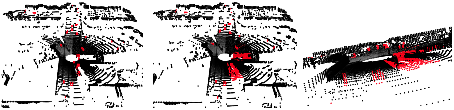
Figure 1: Static background points are shown in black. 1) Left: Dynamic LiDAR scan with occluding dynamic points in red. 2) Center: Static LiDAR scan reconstructed by DSLR. Although DSLR reconstructs complete scan only in-painted dynamic points are shown in red. 3) Right: Reconstructed static LiDAR scan shown from a different angle to highlight reconstruction quality of 3D structures like walls.

We show that existing techniques for non-LiDAR data produce sub-optimal reconstructions for LiDAR data (Caccia et al. 2018; Achlioptas et al. 2017; Groueix et al. 2018). However, downstream tasks such as SLAM in a dynamic environment require accurate and high-quality LIDAR scans.

To address these shortcomings, we propose a Dynamic to Static LiDAR Reconstruction (DSLR) algorithm. It uses an autoencoder that is adversarially trained using a discriminator to reconstruct corresponding static frames from dynamic frames. Unlike existing DST based methods, DSLR doesn’t require specific segmentation annotation to identify dynamic points. We train DSLR using a dataset that consists of corresponding dynamic and static scans of the scene. However, these pairs are hard to obtain in a simulated environment and even harder to obtain in the real world. To get around this, we also propose a new algorithm to generate appropriate dynamic and static pairs which makes DSLR the first DST based model to train on a real-world dataset.

We now summarize the contributions of our paper:

• This paper initiates a study of DST for LiDAR scans and establishes that existing methods, when adapted to this problem, yield poor reconstruction of the underlying static environments. This leads to extremely poor performance in down-stream applications such as SLAM. To address this research gap we develop DSLR, an adversarially trained autoencoder which learns a mapping from the latent space of dynamic scans to their static counterparts. This mapping is made possible due to the use of a pair-based discriminator, which is able to distinguish between corresponding static and dynamic scans. Experiments on simulated and real-world datasets show that DSLR gives at least a $4\times$ improvement over adapted baselines.

• DSLR does not require segmentation information. However, if segmentation information is available, we propose an additional variant of our model DSLR-Seg. This model leverages the segmentation information and achieve an even higher quality reconstruction. To ensure that DSLR works in scenarios where corresponding dynamic-static scan pairs might not be easily available, we utilise methods from unsupervised domain adaptation to develop DSLR-UDA.

• We show that DSLR, when compared to other baselines, is the only model to have its reconstruction quality fall within the acceptable limits for SLAM performance as shown in our experiments.

• We open-source 2 new datasets, CARLA-64, ARD-16 (Ati Realworld Dataset) consisting of corresponding static-dynamic LiDAR scan pairs for simulated and real world scenes respectively. We also release our pipeline to create such datasets from raw static and dynamic runs.

2 Related Work

Point Set Generation Network (Fan, Su, and Guibas 2017) works on 3D reconstruction using a single image, resulting in output point set coordinates that handle ambiguity in image ground truth effectively. PointNet (Qi et al. 2017) enables direct consumption of point clouds without voxelization or other transformations and provides a unified, efficient and effective architecture for a variety of down stream tasks. Deep generative models (Achlioptas et al. 2017) have attempted 3D reconstruction for point clouds and the learned representations in these models outperform existing methods on 3D recognition tasks. AtlasNet (Groueix et al. 2018) introduces an interesting method to generate shapes for 3D structures at various resolutions with improved precision and generalization capabilities.

Recent approaches also explore the problem of unpaired point cloud completion using generative models (Chen, Chen, and Mitra 2019). They demonstrate the efficacy of their method on real life scans like ShapeNet. They further extend their work to learn one-to-many mapping between an incomplete and a complete scan using generative modelling (Wu et al. 2020). Deep generative modelling for LiDAR scan reconstruction was introduced through the use of Conditional-GAN (Caccia et al. 2018). The point clouds generated in LiDAR scans are different from normal point clouds. Unlike the latter, they give a 360°view of the surrounding and are much more memory intensive, rich in detail and complex to work with. While most deep generative models for 3D data focus on 3D reconstruction, few attempts have been made to use them for DST. Empty-Cities (Bescos et al. 2018) uses a conditional GAN to convert images with dynamic content into realistic static images by in-painting the occluded part of a scene with a realistic background.

3 Methodology

Given a set of dynamic frames $D=\{d_{i}:i=1,\dots,n\}$, and their corresponding static frames $S=\{s_{i}:i=1,\dots,n\}$, our aim is to find a mapping between the latent space of dynamic frames to its corresponding static frames while preserving the static-structures in $D_{i}$ and in-painting the regions occluded by dynamic-objects with the static-background. Our model consists of 3 parts: (a) An autoencoder trained to reconstruct LiDAR point clouds (Caccia et al. 2018), (b) A pair discriminator to distinguish ($S_{i},S_{j}$) pairs from ($S_{i},D_{j}$). Inspired by (Denton et al. 2017), the discriminator is trained using latent embedding vector pairs obtained using standard autoencoder as input, (c) An adversarial model that uses the above 2 modules to learn an autoencoder that maps dynamic scans to corresponding static scans.

We also describe $2$ variants of our models for (a) unsupervised domain adaptation to new environments, (b) utilizing segmentation information if available. For all following sections, x refers to a LiDAR range image (transformed to a single column vector), $r(x)$ represent the the latent representation, $\overline{x}$ represents the reconstructed output, xⁱ refers to a component of x.

DSLR: Dynamic to Static LiDAR Scan Reconstruction

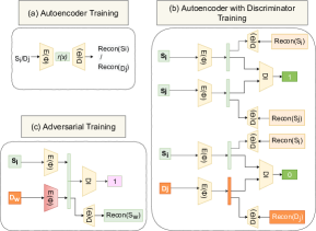
Figure 2: Model architecture. (a) Autoencoder (G) is trained to reconstruct LiDAR point clouds. (b) Discriminator (DI) is trained to discriminate $(x\in S,y\in S),(x\in S,y\in D)$ LiDAR scan pairs (c) Adversarial training using G and DI where $D_{w}$ and $S_{i}$ are corresponding dynamic-static pairs.

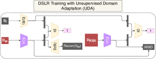
Figure 3: Adversarial training along with UDA for domain adaptation on KITTI data. Purple color indicate trainable weights. Refer Section 3.

The details of our model architecture and pipeline are illustrated in Fig. 2.

Input Preprocessing:

We use the strategy described by (Caccia et al. 2018) for converting LiDAR point clouds into range images.

Autoencoder:

The Encoder ($E_{\phi}$) and Decoder ($D_{\theta}$) are based on the discriminator and generator from DCGAN (Radford, Metz, and Chintala 2015) as adapted in (Caccia et al. 2018). However, we change the model architecture to a $40\times 512$ grid instead of a $64\times 1024$ grid. This is done to discard the outer circles in a LiDAR scan because it contains the most noise and have least information about the scene. The bottleneck dimension of our model is $160.$ We define the network G as,

$$G:x\xrightarrow[]{E_{\phi}}r(x)\xrightarrow[]{D_{\theta}}\overline{x}\quad$$ (1)

The autoencoder $G_{\phi,\theta}$ is trained with all s_i, d_j to reconstruct a given input at the decoder. We use a pixel-wise reconstruction loss for the LiDAR based range-image.

$$\operatorname{MSE}(x,\overline{x})=\|x-\overline{x}\|^{2}$$ (2)

The autoencoder tries to learns the optimal latent vector representations $r(x)$ for static and dynamic LiDAR scans for efficient reconstruction. For ease of representation in the rest of the paper we omit the usage of parameters $\phi$ and $\theta$ for encoder and decoder of $G$, and they should be considered implicitly unless specified otherwise.

Adversarial Model

Pair Discriminator

We use a feed-forward network based discriminator (DI). DI takes random scan pairs ($s_{i},s_{j}$) and ($s_{i}$, $d_{j}$) and transforms them to latent vector pairs using $G.$ It is trained to output $1$ if both latent vectors represent static LiDAR scans, else $0$.

$$DI\left(r(x_{1}),\left(r(x_{2}\right)\right)=\left\{\begin{array}[]{ll}1&x_{1}\in S,x_{2}\in S\\ 0&x_{1}\in S,x_{2}\in D\\ \end{array}\right\}$$ (3)

The discriminator is trained using Binary Cross-Entropy (BCE) Loss between $\overline{y}$ and $y$, where $\overline{y}$ denotes the discriminator output and $y$ denotes the ground truth.

Corresponding static and dynamic LiDAR frames look exactly the same except for the dynamic-objects and holes present in the latter. It is hard for the discriminator to distinguish between these two because of minimal discriminatory features present in the pairs. To overcome this, we use a dual-loss setting where we jointly train the already pre-trained autoencoder G along with discriminator. Therefore, the total loss is the sum of MSE Loss of autoencoder and BCE loss of discriminator. Using reconstruction loss not only helps in achieving training stability but also forces the encoder to output a latent vector that captures both generative and discriminative features of a LiDAR scan. We represent the loss as $L\textsubscript{DI}.$ For simplicity, we present $L\textsubscript{DI}$ for only one set of input data ($x_{1},{x}_{2},{x}_{3}$), where ${x}_{1},{x}_{2}\in S$, ${x}_{3}\in D$.

$$\begin{split}L_{DI}=&MSE({x}_{1},\overline{{x}_{1}})+MSE({x}_{2},\overline{{x}_{2}})+MSE({x}_{3},\overline{{x}_{3}})\\ &+BCE(DI(r({x}_{1}),r({x}_{2})),1)\\ &+BCE(DI(r({x}_{1}),r({x}_{3})),0)\end{split}$$ (4)

Adversarial Training:

In the adversarial training, we create two copies of the autoencoder represented as $G^{1}_{\phi_{1},\theta_{1}}$ and $G^{2}_{\phi_{2},\theta_{2}}$. We freeze $\phi_{1}$, $\theta_{1}$, $\theta_{2}$, leaving only $\phi_{2}$ of $G^{2}$ trainable. Inputs ${{x}_{1}\in S,{{x}_{2}}\in D}$ are passed through $G^{1}$ and $G^{2}$ respectively, which output $r({x}_{1})$ and $r({x}_{2})$. These outputs are the latent representations of the static and dynamic scans. We concatenate $r({x}_{1})$ and $r({x}_{2})$ and feed it to the discriminator. DI should ideally output $0$ as shown in Eq. 3. However, in an adversarial setting, we want to fool the discriminator into thinking that both the vectors belong to $S$ and hence backpropagate the BCE loss w.r.t target value $1$, instead of $0.$ As training progresses the encoder weights for $G^{2}$, i.e. $\phi_{2}$, are updated to produce a static latent vector for a given dynamic frame, learning a latent vector mapping from dynamic scan to static scan. Additionally, we also backpropagate the reconstruction loss MSE(${x}_{2}$, $\overline{{x}_{2}}$), which ensures that $G^{2}$ generates the nearest corresponding static latent representation $z$ when given dynamic frame ${x}_{2}$ as input. The corresponding static scan reconstruction obtained from $z$ using $\theta_{2}$ in such a setting is qualitatively and quantitatively better than what would have been obtained through a simple dynamic-to-static reconstruction based autoencoder, as shown in Table 1. We represent the adversarial loss as L_A. Here, M denotes the total number of latent vector pairs used to train DI.

$$\begin{split}L_{A}(s_{i},d_{j})=\sum_{i=1}^{M}\sum_{j=i+1}^{M}-\log(DI(r(s_{i}),r(d_{j})))\\ +MSE(s_{i},\overline{d_{j}})\end{split}$$ (5)

Figure 4: DSLR-Seg For a given dynamic frame, DSLR gives us static reconstruction and we use U-Net to get a static segmentation mask. We substitute dynamic points with reconstructed static points and take static points from the given dynamic frame for the final reconstruction.

DSLR-UDA

Due to the unavailability of ground truth static scans S for corresponding D, training DSLR on real-world data is often not possible. A model trained on a simulated dataset usually performs poorly on real-world datasets due to the inherent noise and domain shift.

To overcome this, we use Unsupervised Domain Adaptation (UDA) for adapting DSLR to real world datasets where paired training data is unavailable.

In UDA, we have two domains: source and target. Source domain contains the output labels while the target domain does not. We take inspiration from (Tzeng et al. 2014) that uses a shared network with a Maximum Mean Discrepancy (MMD) (Borgwardt et al. 2006) loss that minimizes the distance between the source and target domain in the latent space.

MMD loss is added to the adversarial phase of the training as shown in Fig. 3. Latent vectors from the dynamic-source and dynamic-target scans are used to calculate the MMD loss. For more details refer to Section 1.5 in Appendix. Latent representations of static-source and target-dynamic scans are also fed to the discriminator with adversarial output as $1$, instead of $0$. All weights except for the encoder in blue, in Fig. 3, are frozen. The following equation denotes adversarial loss with UDA, L_U:

$$\begin{split}L_{U}=&L_{A}({s}_{i},{d}_{j})+\lambda\sum_{i=1}^{M}\sum_{j=i+1}^{M}MMD^{2}(r({d}_{j}),r({k}_{j}))\end{split}$$ (6)

where, $\textbf{s}_{i}$ $\in$ $S$, ${d}_{j}$ $\in$ $D$ in source domain, and ${k}_{j}$ represents dynamic scan in target domain. $\lambda$ is a constant which is set to 0.01.

DSLR-Seg

Although DSLR achieves a high-quality of reconstruction without segmentation information, it can leverage the same to further improve the reconstruction quality. High-quality LiDAR reconstructions are desirable in many downstream applications (e.g SLAM) for accurate perception of the environment. While the output reconstructions of DSLR replace dynamic objects with corresponding static background accurately, it adds some noise in the reconstructed static which is undesirable.

To overcome this, we propose DSLR-Seg, which uses point-wise segmentation information to fill the dynamic occlusion points with the corresponding background static-points obtained from DSLR. To this end, we train a U-Net (Ronneberger, Fischer, and Brox 2015) to segment dynamic and static points in a given LiDAR frame. The U-Net model outputs a segmentation mask.

We consider static-points from the input dynamic-frame and dynamic-points from the reconstructed static-output and generate the reconstructed output as shown in the Figure 4. Mathematically, we can represent the above using Eq. 7.

$$Recon=Mask_{i}*\overline{s_{i}}+(1-Mask_{i})d_{i}$$ (7)

Here, $Mask_{i}$ is a segmentation mask generated by U-Net model consisting values 0 for static and 1 for dynamic points. $d_{i}$ is the input dynamic frame to the model and $\overline{s_{i}}$ is the reconstructed static frame which is given by the model.

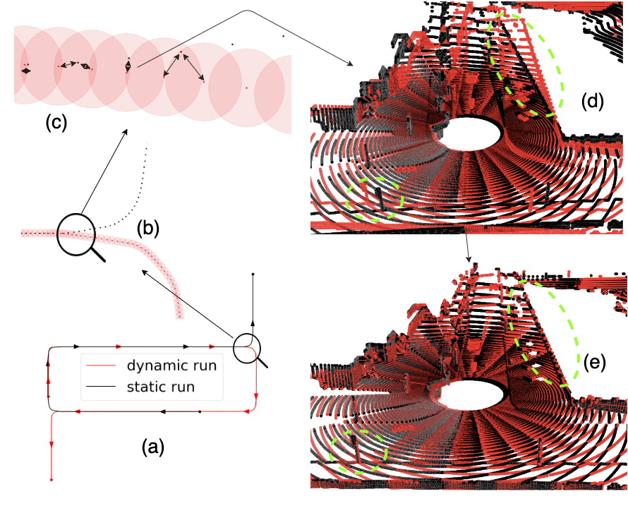
Figure 5: Dataset generation framework. Dynamic scans are shown in red, static scans in black. (a) shows a random dynamic and static run with overlap for few LiDAR poses. (b) zoomed-in portion of an overlapping region. (c) zoomed-in region showing paired correspondences using a bidirectional arrow. (d) shows a dynamic-static paired correspondence which often has significant mismatch (highlighted). (e) scan pair after applying pose transformation.

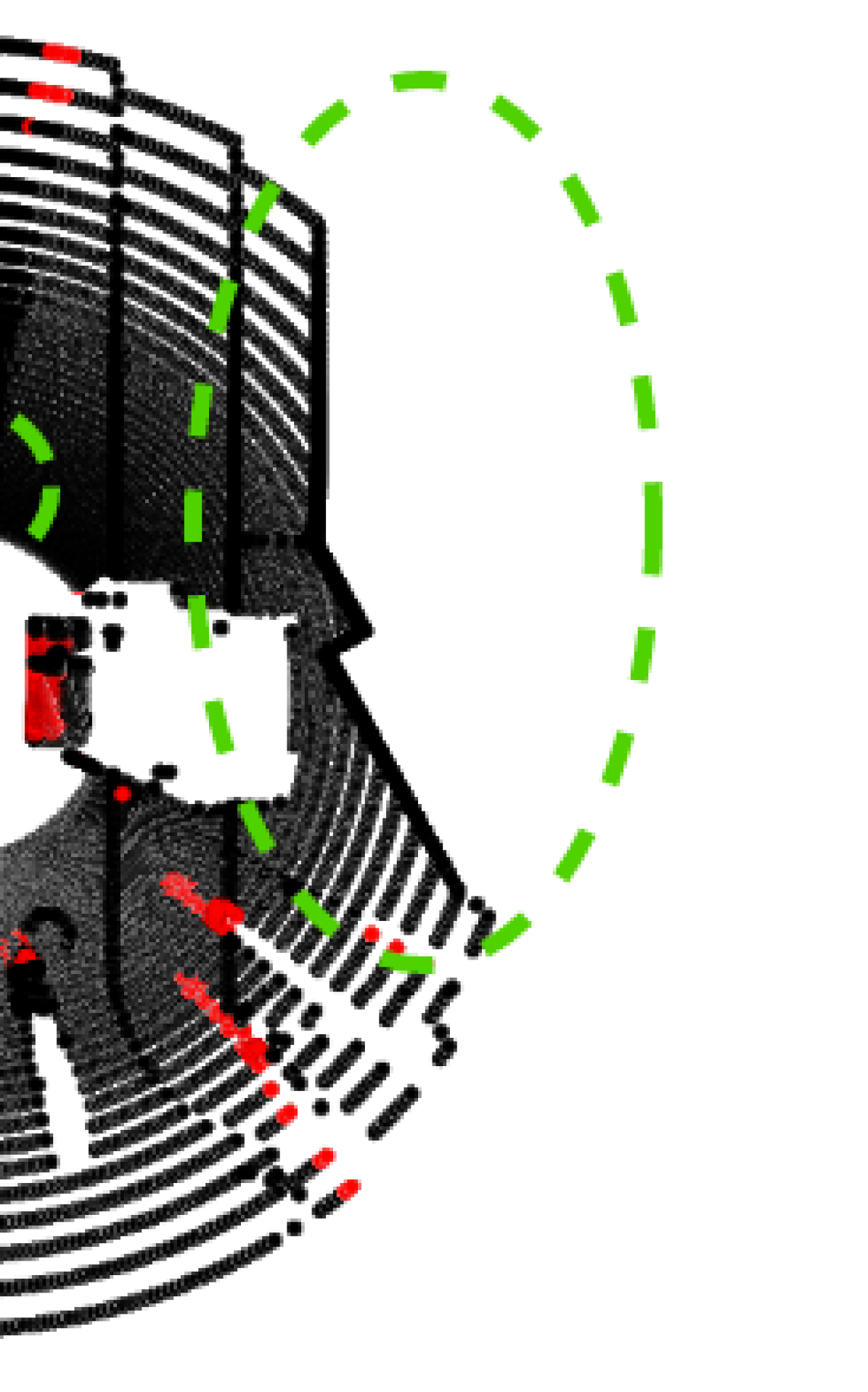
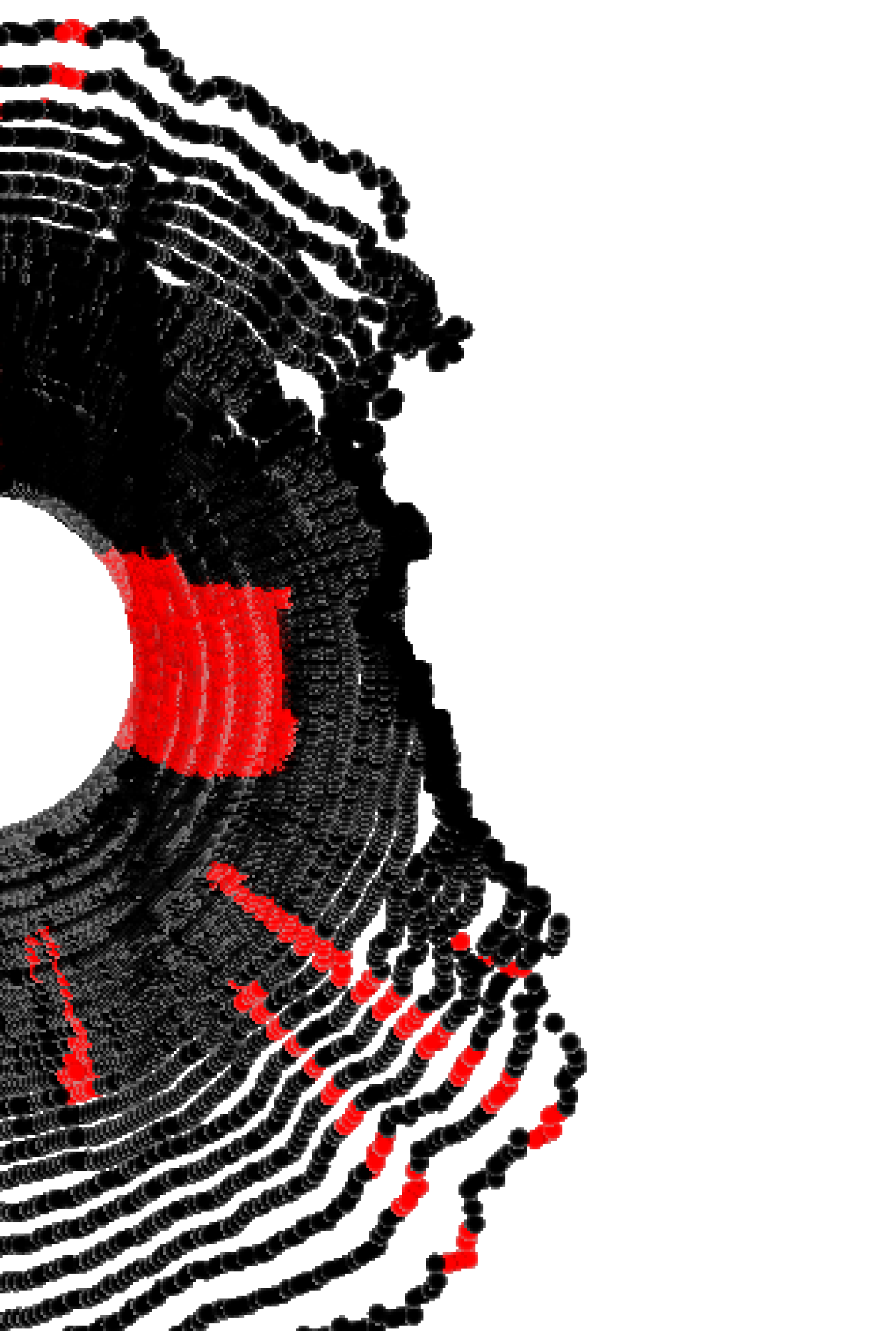
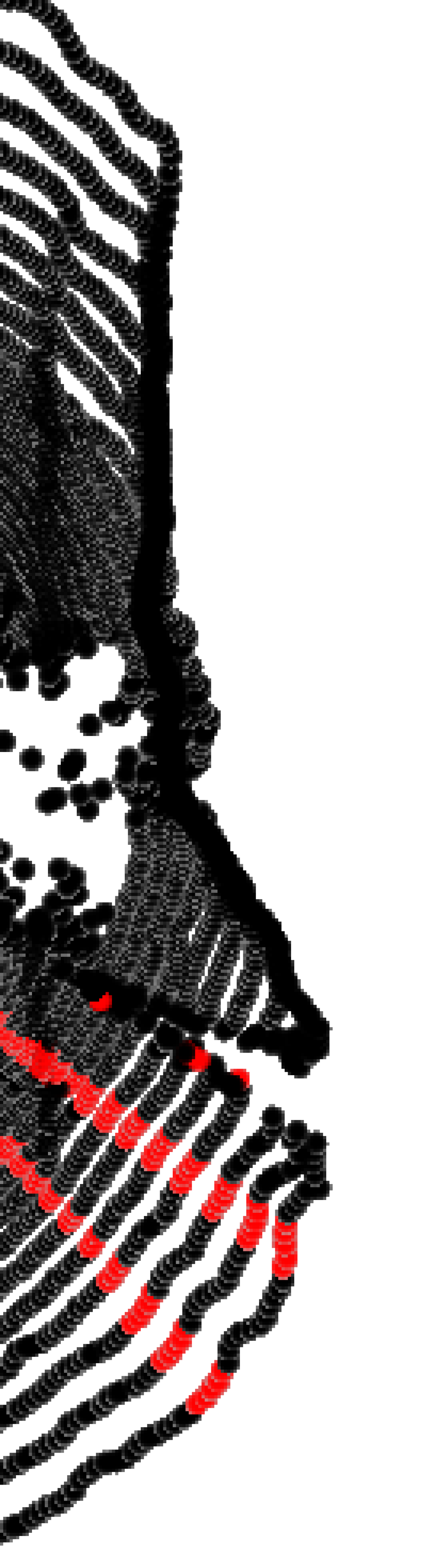
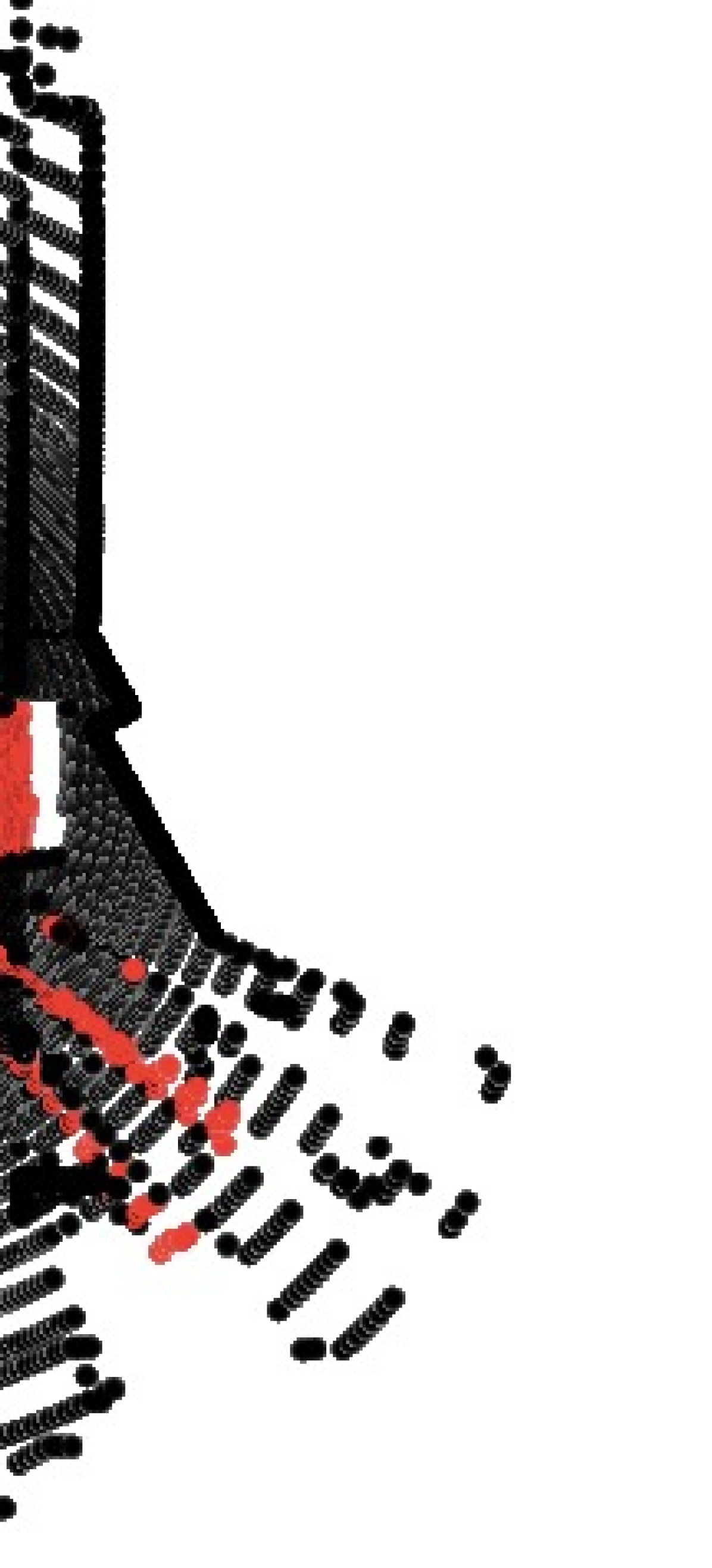
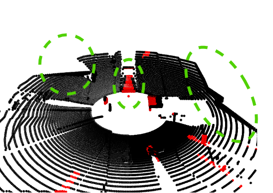
((a)) Dynamic

((b)) ADMG

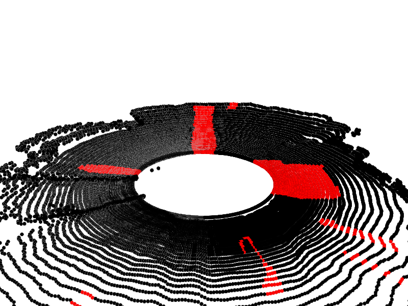
((c)) CHCP-AE

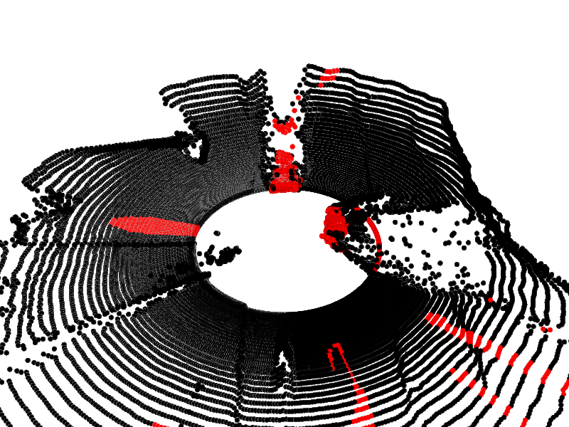
((d)) CHCP-VAE

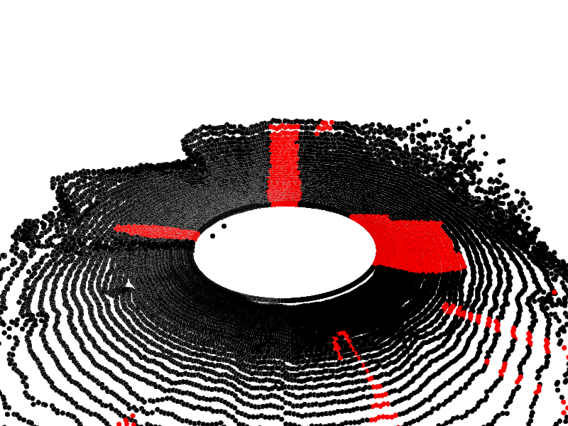
((e)) CHCP-GAN

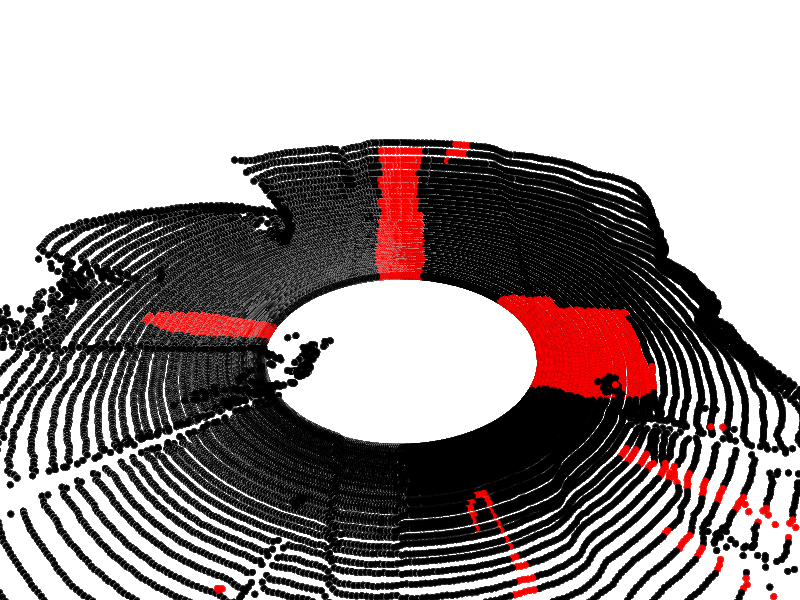
((f)) DSLR

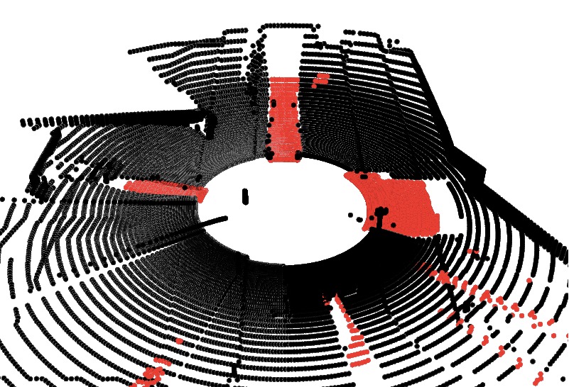
((g)) DSLR-Seg

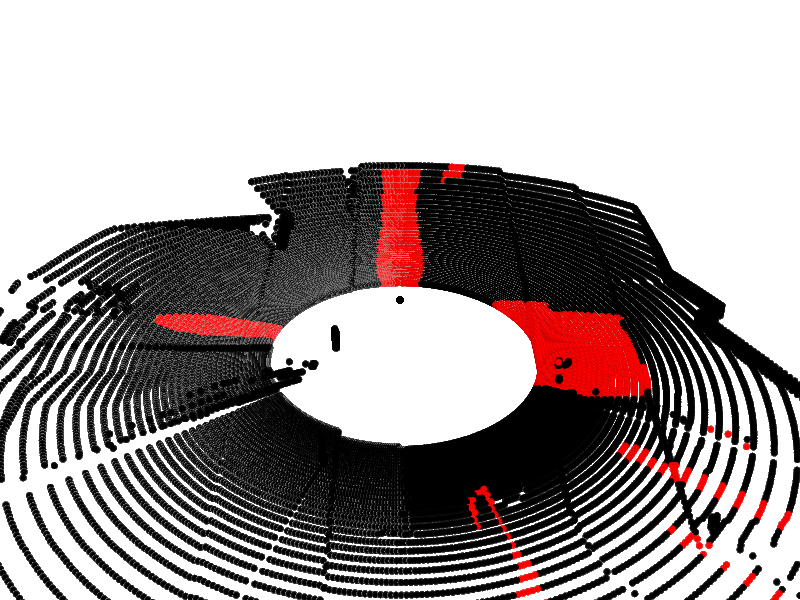
((h)) GT-static

Figure 6: First row shows top-view and bottom row shows lateral view. Reconstruction obtained by DSLR and baseline models on a CARLA-64 scan. Black denotes the static part of the scene. In (a) red denotes dynamic objects, from (b to g) red denotes the reconstructed static background and in (h) red denotes ground truth static. Reconstruction from our model fills occluded regions as well as maintain walls and edges of surrounding scenes clearly compared to the baseline, none of which perform both tasks better compared to DSLR.

Dataset Generation

Set of corresponding static-dynamic LiDAR scan pairs are required, to train DSLR. We propose a novel data-collection framework for obtaining this correspondence. We collect data from 2 runs in the same environment. The first run contains only the static-objects while the second run contains both static and dynamic objects along with the ground-truth poses. Using this, we create pairs of dynamic and its corresponding static-frames. Finally, a relative pose transformation is applied as shown in Figure 5 so that the static structures in both the scans align. All these operations are performed using Open3D (Zhou, Park, and Koltun 2018).

4 Experimental Results

We evaluate our proposed approaches against baselines on three different datasets with the following goals: (1) In section 4, we evaluate our proposed approaches with adapted baseline models for the problem of DST for LiDAR, (2) In section 4, we evaluate our proposed approaches DSLR, DSLR-Seg, and DSLR-UDA, for LiDAR based SLAM. When segmentation information is available, we further improve the quality of our training dataset by identifying the dynamic-points and replace only those points with corresponding static-points obtained from DSLR, as shown in Eq. (7). Based on this, we propose DSLR++, a DSLR model trained on improved dataset created from CARLA-64.

Datasets

CARLA-64 dataset:

We create 64-beam LiDAR dataset with settings similar to Velodyne VLP-64 LiDAR on the CARLA simulator (Dosovitskiy et al. 2017). Similar settings may also improve the model’s generalizability by improving performance on other real-world datasets created using similar LiDAR sensors such as KITTI (Geiger, Lenz, and Urtasun 2012).

KITTI-64 dataset:

To show results on a standard real-world dataset, we use the KITTI odometry dataset (Geiger, Lenz, and Urtasun 2012), which contains segmentation information and ground truth poses.

For KITTI, we cannot build a dynamic-static correspondence training dataset using our generation method due to a dearth of static LiDAR scans (less than 7%) coupled with the fact that most static-scan poses do not overlap with dynamic-scan poses.

ARD-16:

We create ARD-16 (Ati Realworld Dataset), a first of its kind real-world paired correspondence dataset, by applying our dataset generation method on 16-beam VLP-16 Puck LiDAR scans on a slow-moving Unmanned Ground Vehicle. We obtain ground truth poses by using fine resolution brute force scan matching, similar to Cartographer. (Hess et al. 2016).

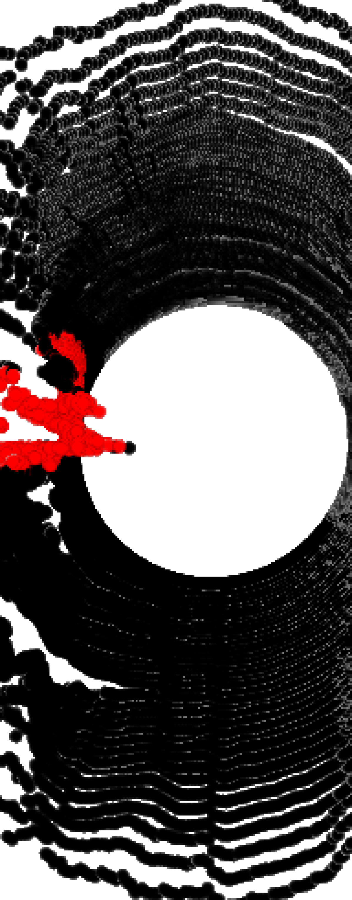
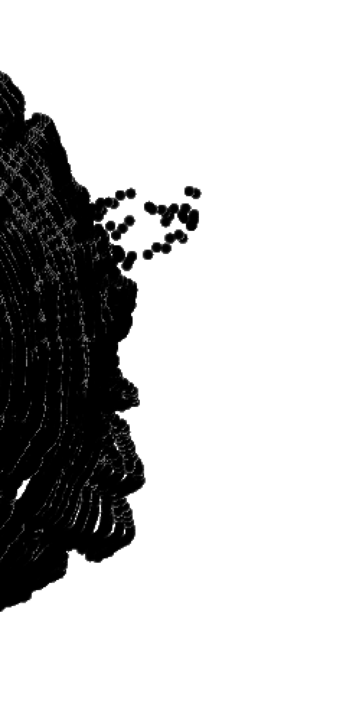
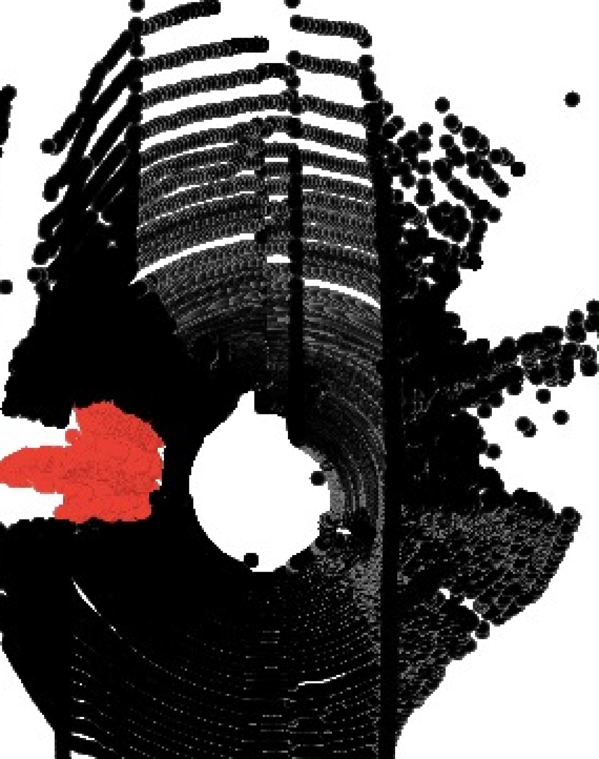
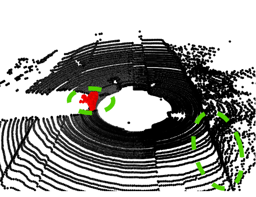
((a)) Dynamic

((b)) ADMG

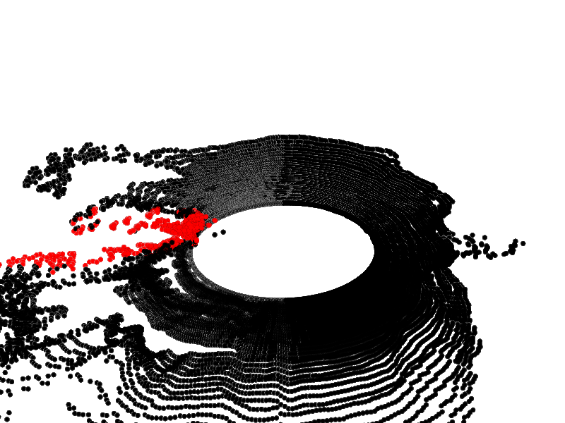
((c)) CHCP-AE

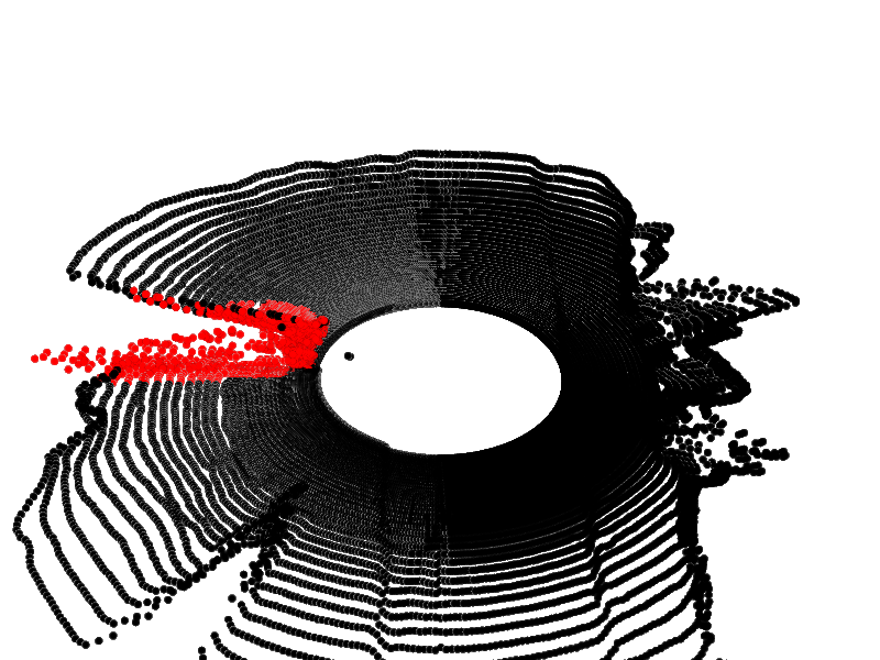
((d)) CHCP-VAE

((e)) CHCP-GAN

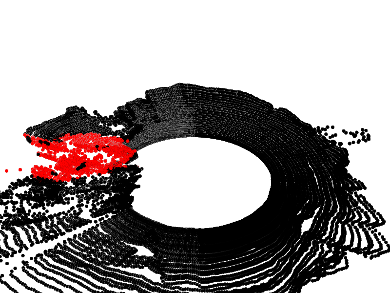
((f)) DSLR

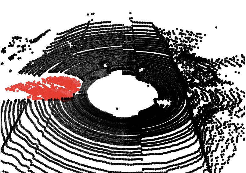
((g)) DSLR-Seg

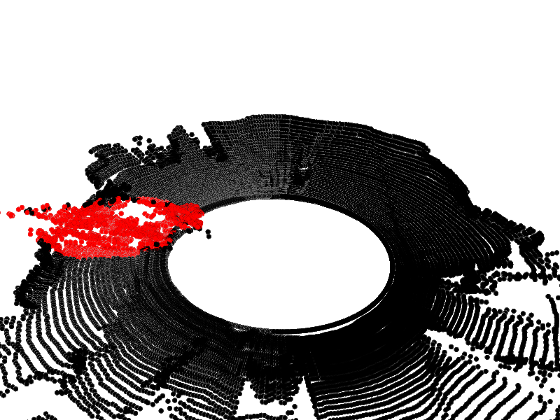
((h)) DSLR-UDA

Figure 7: Reconstruction comparison of DSLR along with UDA. Note that KITTI doesn’t have the corresponding static. Although CHCP-VAE appears to reconstruct well, it is not able to fill dynamic holes, while DSLR-Seg and DSLR-UDA is able to do both.

Dynamic to Static Translation (DST) on LiDAR Scan

Baselines

It is established in the existing literature (Kendall, Grimes, and Cipolla 2015; Krull et al. 2015; Bescos et al. 2019) that learning-based methods significantly outperform non-learning based methods. Hence we adapt the following related work as baselines which leverage learning for reconstruction: (1) AtlasNet(Groueix et al. 2018) (2) ADMG (Achlioptas et al. 2017) (3) CHCP-AE, CHCP-VAE, CHCP-GAN(Caccia et al. 2018) (4) WCZC(Wu et al. 2020) (5) EmptyCities(Bescos et al. 2019). For more details on baselines, refer Section 2.

Evaluation Metrics

We evaluate the difference between the model-reconstructed static and ground-truth static LiDAR scans on CARLA-64 and ARD-16 datasets using 2 metrics : Chamfer Distance(CD) and Earth Mover Distance(EMD) (Hao-Su 2017). For more details refer Section 1.4 in Appendix .

KITTI-64 does not have corresponding ground truth static, thus we propose a new metric, LiDAR scan Quality Index (LQI) which estimates the quality of reconstructed static LiDAR scans by explicitly regressing the amount of noise in a given scan. This has been adapted from the CNN-IQA model (Kang et al. 2014) which aims to predict the quality of images as perceived by humans without access to a reference image. For more details refer Section 1.6 in Appendix.

DST on CARLA-64:

We report static LiDAR reconstruction results in Table 1 and show that DSLR outperforms all baselines and gives at least 4x improvement on CD over adapted CHCP-AE, existing state of the art for DST on LiDAR. Unlike WCZC and EmptyCities, which use segmentation information, DSLR outperforms these without using segmentation information. When segmentation information is available, we extend DSLR to DSLR++ and DSLR-Seg which further improves reconstruction performance. For visual comparison, we show the static LiDAR reconstructions in Fig. 6 generated by our approaches (DSLR and DSLR-Seg) and best performing adapted works (CHCP-AE, CHCP-VAE, CHCP-GAN, ADMG) on CARLA-64 and KITTI-64. Closer inspection of regions highlighted by dashed green lines shows that DSLR and DSLR-Seg accurately in-paint the static background points (shown in red) effectively.

Improved reconstructions using DSLR are due to the imposition of the static structure not only using the reconstruction loss in the image space but also on latent space by forcing the encoder to output latent vector in static domain using discriminator as an adversary. Therefore compared to CHCP-AE, which only uses a simple autoencoder, our use of a discriminator helps identify patterns that help to distinguish the static-dynamic pairs. Also, unlike EmptyCities (Bescos et al. 2019), we work directly on the latent space to map dynamic to static point-clouds, rather than working on the pixel/image space.

DST on KITTI-64:

Due to the unavailability of paired correspondence, models trained on CARLA-64 are tested on KITTI-64 dataset. To adapt to the KITTI-64, we train DSLR using UDA only for DSLR-UDA. Since the ground-truth static is not available, we use the proposed LQI to estimate the quality of reconstructed static LiDAR scans and report the results in Table 1. We plot LQI v/s CD in Fig. 8 and further show that LQI positively correlates with CD on CARLA-64. For more details, refer Table 1 in Appendix.

We show that our approaches, DSLR, DSLR-Seg, and DSLR-UDA outperforms the adapted CHCP-VAE, the best performing baseline on KITTI-64 based on LQI. In Table 1 and Figure 7, we show that although CHCP-VAE is the best performing baseline but like all other baselines, it fails to in-paint accurately. On the contrary, our approach tries to retain the static 3D structures as much as possible and in-paint them accurately. DSLR-UDA trained on KITTI-64 in an unsupervised manner does a better job at recovering road boundaries in LiDAR scan than DSLR. We can also see that using segmentation information, DSLR-Seg is able to perfectly recover static structures like walls and road boundaries.

Model	CARLA-64	ARD-16	KITTI-64
	Chamfer	Chamfer	LQI
AtlasNet	5109.98	176.46	-
ADMG	6.23	1.62	2.911
CHCP-VAE	9.58	0.67	1.128
CHCP-GAN	8.19	0.38	1.133
CHCP-AE	4.05	0.31	1.738
WCZC	478.12	-	-
EmptyCities	29.39	-	-
DSLR (Ours)	1.00	0.20	1.120
DSLR++ (Ours)	0.49	-	-
DSLR-Seg (Ours)	0.02	-	-
DSLR-UDA(Ours)	-	-	1.119

Table 1: Comparison of LiDAR reconstruction baselines on different datasets. Lower is better. Models that require segmentation information have been italicised for reference.

Model	ATE	Drift	RPE
			Trans	Rot
KITTI-64 Dataset
Pure-Dynamic	11.809	14.970	1.620	1.290°
Detect & Delete (MS)	12.490	13.599	1.623	1.290°
Detect & Delete (GTS)	11.458	22.856	1.630	1.336°
DSLR-Seg (MS)	99.642	34.372	1.610	1.290°
DSLR-Seg (GTS)	11.699	19.67	1.620	1.295°
CARLA-64 Dataset
Pure-Dynamic	10.360	18.580	0.056	0.403°
Detect & Delete (MS)	10.430	18.870	0.060	0.430°
Detect & Delete (GTS)	11.650	24.430	0.063	0.401°
DSLR-Seg (MS)	10.760	17.430	0.050	0.390°
DSLR-Seg (GTS)	7.330	13.63	0.050	0.340°
ARD-16 Dataset
Pure-Dynamic	1.701	–	0.036	0.613°
DSLR (Ours)	1.680	–	0.035	0.614°

Table 2: Comparison of SLAM performance with existing Baselines.

DST on ARD-16:

In Table 1, we also report static LiDAR scan reconstruction results on ARD-16 dataset. We do not report results on EmptyCities, WCZC, DSLR++, DSLR-Seg due to the unavailability of segmentation information. To the best of the author’s knowledge, we are the first to train and test a DST based model on real-world data owing to the dataset generation pipeline described in Section 3. We show that DSLR outperforms adapted baselines on all metrics on this dataset and demonstrate the practical usefulness of our method in real-world setting.

We summarize the results of DSLR on the 3 datasets here. We conclude that DSLR gives significant improvement over the best performing baseline model CHCP-AE over both metrics. Moreover, if segmentation information is available, our variants DSLR++ and DSLR-Seg further extend the gains as shown in Table 1. We also show the efficacy of our model on a real world dataset, ARD-16, where our model performs significantly better. We do not have segmentation information available for ARD-16. If segmentation information is available for the real world dataset, the gains can be higher. For a detailed comparison of LiDAR reconstruction baselines refer Table 1 in Appendix.

Application of LiDAR Scan Reconstruction for SLAM in Dynamic Environments

We use Cartographer (Hess et al. 2016), a LiDAR based SLAM algorithm (Filipenko and Afanasyev 2018; Yagfarov, Ivanou, and Afanasyev 2018) to test the efficacy of our proposed approaches DSLR and DSLR-Seg on tasks pertaining to autonomous navigation. Our reconstructed output serves as the input LIDAR scan for Cartographer, which finally gives a registered map of the environment and position of the vehicle in real-time.

Baselines:

We evaluate our model with two baselines: (1) A unprocessed dynamic frame (Pure-Dynamic) and (2) With an efficient LiDAR pre-processing step for handling SLAM in dynamic environment which removes the dynamic points from the LiDAR scan (Detect & Delete) (Ruchti and Burgard 2018; Vaquero et al. 2019).

Evaluation Metrics:

After coupling the Cartographer with above prepossessing steps, the generated output (position of the vehicle) is compared on widely used SLAM metrics like Absolute Trajectory Error (ATE) (Sturm et al. 2012), Relative Position Error (RPE) (Sturm et al. 2012) and Drift. For more details refer Section 3 in Appendix.

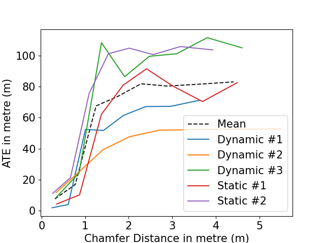
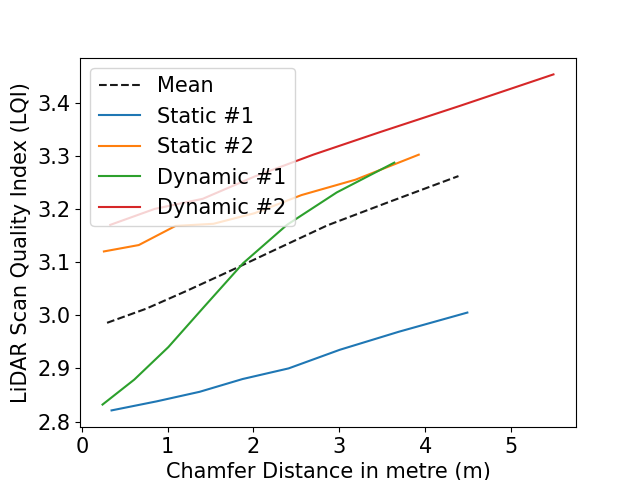
Figure 8: Studying effect of different metrics on Chamfer distance. Left: ATE vs CD plot Right: LQI vs CD plot

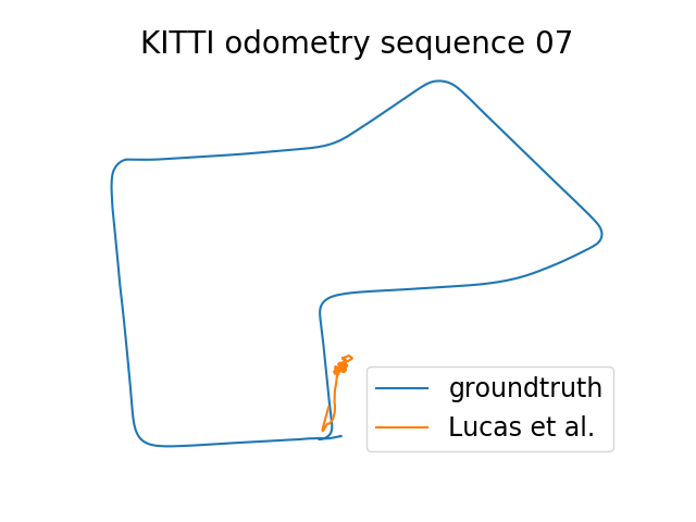
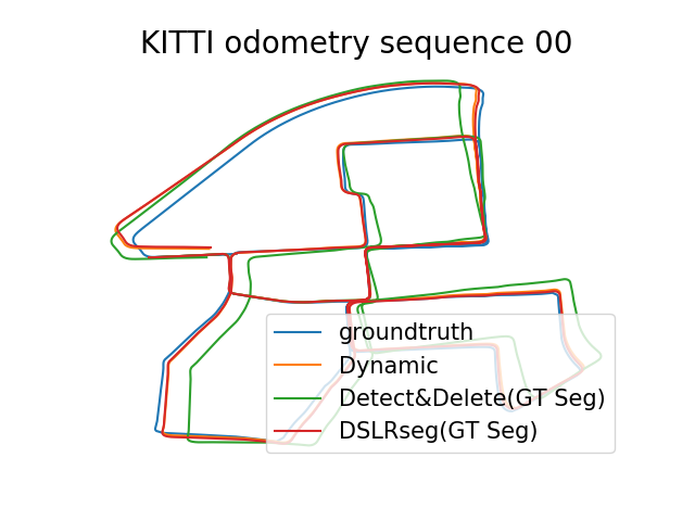
Figure 9: (1) Left: CHCP-AE baseline with ground truth evaluation on KITTI (2) Right: Detect & Delete baseline and DSLR-Seg with Model-Seg variation on KITTI.

Discussion

We compare our best performing model in each dataset against dynamic SLAM baseline methods. We report results with two variations of segmentation for CARLA-64 and KITTI-64 to limit the effect of segmentation inaccuracy in our interpretation. We report MS variant when U-Net was used to give segmentation masks for dynamic points and GTS variation when ground truth segmentation masks were used. In Table 2, we show that our approaches outperform the base case Pure-Dynamic in most of the cases and perform competitively against dynamic SLAM baseline. We choose DSLR-Seg for comparison on CARLA-64 and KITTI-64 and DSLR for comparison on ARD-16 due to the unavailability of segmentation information for ARD-16. For a detailed analysis refer to Section 3 of the Appendix.

We also study the relation between LiDAR reconstruction error (CD) and SLAM error (ATE). For this, we take random dynamic and static scans from CARLA-64 dataset and linearly increase LiDAR reconstruction error by corrupting them with Gaussian noise and report SLAM errors for the same. In Figure 8, we observe that for most runs, SLAM error initially increases exponentially with linear increase in LiDAR error and then saturates at a CD of 2m. Based on this, we conclude that, for any reconstruction model to be practical for SLAM, it must have reconstruction error or CD below 2m which we refer to it as SLAM Reconstruction Threshold (SRT). We see from CARLA-64 results in Table 1 that DSLR is the only model to have its reconstruction error below the SRT and therefore is practically feasible for SLAM. We show this experimentally by plotting the trajectory estimated by CHCP-VAE, the best performing static LiDAR scan reconstruction baseline in Figure 9 and show that pose estimated by Cartographer gets stuck after some time due to high LiDAR reconstruction error, making it impractical.Through this study we establish the superiority of our proposed models over existing approaches in static LiDAR scan reconstruction for SLAM.

5 Conclusion

We propose a novel, adversarially-trained, autoencoder model for static background LiDAR reconstruction without the need of segmentation masks. We also propose variants that accept available segmentation masks for further improving LiDAR reconstruction. It also enhances SLAM performance in dynamic environments. However some drawbacks in our reconstruction are discussed in Appendix. Future work to address those issues can help improve the reconstruction quality even more and their applicability for tasks in real world environments.

References

- Achlioptas et al. (2017) Achlioptas, P.; Diamanti, O.; Mitliagkas, I.; and Guibas, L. 2017. Representation learning and adversarial generation of 3d point clouds. arXiv preprint arXiv:1707.02392 .
- Bescos et al. (2018) Bescos, B.; Fácil, J. M.; Civera, J.; and Neira, J. 2018. DynaSLAM: Tracking, mapping, and inpainting in dynamic scenes. IEEE Robotics and Automation Letters 3(4): 4076–4083.
- Bescos et al. (2019) Bescos, B.; Neira, J.; Siegwart, R.; and Cadena, C. 2019. Empty cities: Image inpainting for a dynamic-object-invariant space. In 2019 International Conference on Robotics and Automation (ICRA), 5460–5466. IEEE.
- Bešić and Valada (2020) Bešić, B.; and Valada, A. 2020. Dynamic Object Removal and Spatio-Temporal RGB-D Inpainting via Geometry-Aware Adversarial Learning. arXiv preprint arXiv:2008.05058 .
- Biasutti et al. (2017) Biasutti, P.; Aujol, J.-F.; Brédif, M.; and Bugeau, A. 2017. Disocclusion of 3D LiDAR point clouds using range images.
- Borgwardt et al. (2006) Borgwardt, K.; Gretton, A.; Rasch, M. J.; Kriegel, H.; Schölkopf, B.; and Smola, A. 2006. Integrating structured biological data by Kernel Maximum Mean Discrepancy. Bioinformatics 22 14: e49–57.
- Caccia et al. (2018) Caccia, L.; van Hoof, H.; Courville, A.; and Pineau, J. 2018. Deep generative modeling of lidar data. arXiv preprint arXiv:1812.01180 .
- Chen, Chen, and Mitra (2019) Chen, X.; Chen, B.; and Mitra, N. J. 2019. Unpaired point cloud completion on real scans using adversarial training. arXiv preprint arXiv:1904.00069 .
- Chen et al. (2019) Chen, X.; Milioto, A.; Palazzolo, E.; Giguère, P.; Behley, J.; and Stachniss, C. 2019. SuMa++: Efficient LiDAR-based semantic SLAM. In 2019 IEEE/RSJ International Conference on Intelligent Robots and Systems (IROS), 4530–4537. IEEE.
- Denton et al. (2017) Denton, E. L.; et al. 2017. Unsupervised learning of disentangled representations from video. In Advances in neural information processing systems, 4414–4423.
- Dosovitskiy et al. (2017) Dosovitskiy, A.; Ros, G.; Codevilla, F.; Lopez, A.; and Koltun, V. 2017. CARLA: An Open Urban Driving Simulator. In Proceedings of the 1st Annual Conference on Robot Learning, 1–16.
- Fan, Su, and Guibas (2017) Fan, H.; Su, H.; and Guibas, L. J. 2017. A point set generation network for 3d object reconstruction from a single image. In Proceedings of the IEEE conference on computer vision and pattern recognition, 605–613.
- Filipenko and Afanasyev (2018) Filipenko, M.; and Afanasyev, I. 2018. Comparison of various slam systems for mobile robot in an indoor environment. In 2018 International Conference on Intelligent Systems (IS), 400–407. IEEE.
- Geiger, Lenz, and Urtasun (2012) Geiger, A.; Lenz, P.; and Urtasun, R. 2012. Are we ready for autonomous driving? the kitti vision benchmark suite. In 2012 IEEE Conference on Computer Vision and Pattern Recognition, 3354–3361. IEEE.
- Groueix et al. (2018) Groueix, T.; Fisher, M.; Kim, V. G.; Russell, B. C.; and Aubry, M. 2018. A papier-mâché approach to learning 3d surface generation. In Proceedings of the IEEE conference on computer vision and pattern recognition, 216–224.
- Hao-Su (2017) Hao-Su. 2017. 3d deep learning on point cloud representation (analysis). URL http://graphics.stanford.edu/courses/cs468-17-spring/LectureSlides/L14%20-%203d%20deep%20learning%20on%20point%20cloud%20representation%20(analysis).pdf.
- Hess et al. (2016) Hess, W.; Kohler, D.; Rapp, H.; and Andor, D. 2016. Real-time loop closure in 2D LIDAR SLAM. In 2016 IEEE International Conference on Robotics and Automation (ICRA), 1271–1278. IEEE.
- Kang et al. (2014) Kang, L.; Ye, P.; Li, Y.; and Doermann, D. 2014. Convolutional neural networks for no-reference image quality assessment. In Proceedings of the IEEE conference on computer vision and pattern recognition, 1733–1740.
- Kendall, Grimes, and Cipolla (2015) Kendall, A.; Grimes, M.; and Cipolla, R. 2015. Posenet: A convolutional network for real-time 6-dof camera relocalization. In Proceedings of the IEEE international conference on computer vision, 2938–2946.
- Kim and Kim (2020) Kim, G.; and Kim, A. 2020. Remove, then Revert: Static Point cloud Map Construction using Multiresolution Range Images. In Proceedings of the IEEE/RSJ International Conference on Intelligent Robots and Systems (IROS). Las Vegas. Accepted. To appear.
- Krull et al. (2015) Krull, A.; Brachmann, E.; Michel, F.; Ying Yang, M.; Gumhold, S.; and Rother, C. 2015. Learning analysis-by-synthesis for 6D pose estimation in RGB-D images. In Proceedings of the IEEE international conference on computer vision, 954–962.
- Qi et al. (2017) Qi, C. R.; Su, H.; Mo, K.; and Guibas, L. J. 2017. Pointnet: Deep learning on point sets for 3d classification and segmentation. In Proceedings of the IEEE conference on computer vision and pattern recognition, 652–660.
- Radford, Metz, and Chintala (2015) Radford, A.; Metz, L.; and Chintala, S. 2015. Unsupervised representation learning with deep convolutional generative adversarial networks. arXiv preprint arXiv:1511.06434 .
- Ronneberger, Fischer, and Brox (2015) Ronneberger, O.; Fischer, P.; and Brox, T. 2015. U-net: Convolutional networks for biomedical image segmentation. In International Conference on Medical image computing and computer-assisted intervention, 234–241. Springer.
- Ruchti and Burgard (2018) Ruchti, P.; and Burgard, W. 2018. Mapping with Dynamic-Object Probabilities Calculated from Single 3D Range Scans. In 2018 IEEE International Conference on Robotics and Automation (ICRA), 6331–6336. IEEE.
- Sturm et al. (2012) Sturm, J.; Engelhard, N.; Endres, F.; Burgard, W.; and Cremers, D. 2012. A benchmark for the evaluation of RGB-D SLAM systems. In 2012 IEEE/RSJ International Conference on Intelligent Robots and Systems, 573–580.
- Tzeng et al. (2014) Tzeng, E.; Hoffman, J.; Zhang, N.; Saenko, K.; and Darrell, T. 2014. Deep Domain Confusion: Maximizing for Domain Invariance.
- Vaquero et al. (2019) Vaquero, V.; Fischer, K.; Moreno-Noguer, F.; Sanfeliu, A.; and Milz, S. 2019. Improving Map Re-localization with Deep ‘Movable’Objects Segmentation on 3D LiDAR Point Clouds. In 2019 IEEE Intelligent Transportation Systems Conference (ITSC), 942–949. IEEE.
- Wu et al. (2020) Wu, R.; Chen, X.; Zhuang, Y.; and Chen, B. 2020. Multimodal Shape Completion via Conditional Generative Adversarial Networks. arXiv preprint arXiv:2003.07717 .
- Yagfarov, Ivanou, and Afanasyev (2018) Yagfarov, R.; Ivanou, M.; and Afanasyev, I. 2018. Map comparison of lidar-based 2d slam algorithms using precise ground truth. In 2018 15th International Conference on Control, Automation, Robotics and Vision (ICARCV), 1979–1983. IEEE.
- Zhou, Park, and Koltun (2018) Zhou, Q.-Y.; Park, J.; and Koltun, V. 2018. Open3D: A Modern Library for 3D Data Processing. arXiv:1801.09847 .