Pairing and superconductivity in quasi one-dimensional flat band systems: Creutz and sawtooth lattices

Abstract

We study the pairing and superconducting properties of the attractive Hubbard model in two quasi one-dimensional topological lattices, the Creutz and sawtooth lattices, which share two peculiar properties: each of their band structures exhibits a flat band with a non-trivial winding number. The difference, however, is that only the Creutz lattice is genuinely topological, owing to a chiral (sub-lattice) symmetry, resulting in a quantized winding number and zero energy edge modes for open boundary conditions. We use multi-band mean field and exact density matrix renormalization group in our work. Our three main results are: (a) For both lattice systems, the superconducting weight, $D_{s}$, is linear in the coupling strength, $U$, for low values of $U$; (b) for small $U$, $D_{s}$ is proportional to the quantum metric for the Creutz system but not for the sawtooth system because its sublattices are not equivalent. We have therefore extended the approach to this more complex situation and found a excellent agreement with the numerical results; (c) at moderate and large $U$, conventional BCS mean field is no longer appropriate for such systems with inequivalent sublattices. We show that, for a wide range of densities and coupling strengths, these systems are very well described by a full multi-band mean field method where the pairing parameters and the local particle densities on the inequivalent sublattices are variational mean field parameters.

I Introduction

Systems with dispersionless (flat) bands have been the focus of much interest due to the wide range of exotic quantum phases they can exhibit. In such models, even infinitesimal interactions are much larger than the band width, resulting in strongly correlated physics. This was argued Khodel and Shaginyan (1990); Kopnin et al. (2011); Heikkilä et al. (2011) to lead to much higher critical temperatures for the transition to a superconducting (SC) phase. Interest in such systems intensified dramatically with the discovery of nonconventional SC in bi-layer graphene Cao et al. (2018) twisted at a “magic” angle which causes a flat band to appear in the band structure of the system. The energy of a particle in a flat band is independent of its momentum which results in very high degeneracy and the localization of the particle on a few sites due to destructive quantum interference Schulenburg et al. (2002); Zhitomirsky and Tsunetsugu (2004); Derzhko et al. (2009). For weak attractive interaction (much smaller than the gap between the flat band and other bands), it was argued, using BCS mean field theory (MF), that the SC weight is linearly dependent on the interaction strength Peotta and Törmä (2015); Tovmasyan et al. (2016); Liang et al. (2017); Verma et al. (2021) and proportional to the quantum metric, thereby linking the SC weight to the topological properties of the non-interacting system Provost and Vallée (1980); Berry (1989); Chiu et al. (2016). This was confirmed for the Creutz lattice with exact numerical calculations Mondaini et al. (2018); Tovmasyan et al. (2018) and for a two-dimensional model using determinant quantum Monte CarloHofmann et al. (2020). The main assumption behind this prediction is that the gap function, $\Delta$ (see below), is uniform, which is the case for a class of flat band systems like the Creutz lattice. However, there are other systems of theoretical and experimental interest, such as the sawtooth lattice Pyykkönen et al. (2021), where this assumption is not valid as the gap function and site density are sublattice dependent. It is thus important to identify how these predictions of the dependence on the coupling and quantum metric change. In fact, as we show below, the BCS MF treatment itself needs to be reexamined and modified. In Ref.Mondaini et al. (2018) it was shown that in the large $U$ limit, the attractive Hubbard model on the Creutz lattice is well represented by an effective hard core boson model in a non-flat band and with near neighbor repulsive interactionEmery (1976); Micnas et al. (1990). With the low and high $U$ limits studied, an interesting question arises: Can one calculate the properties of the system in the intermediate coupling regime where $U$ is comparable to the gap between the bands, and where, consequently, there is strong band mixing?

Here, we address these issues by studying superconductivity in the attractive Hubbard model with balanced populations in two quasi one-dimensional lattices which exhibit a flat band in their ground state; the Creutz Creutz (1999) and sawtooth Sen et al. (1996); Nakamura and Kubo (1996) lattices. Our main results are as follows. Using both multi-band BCS MF and exact density matrix renormalization group (DMRG) calculations, we determine the SC weight and the gap functions, and show excellent agreement over a wide range of particle densities and couplings. This is rather remarkable because at very low interaction, the flat band (and lattice topology) determine the physics; at intermediate coupling, $\absolutevalue{U}$ of the order of the gap between the bands, strong inter-band mixing determines the physics; and at very strong coupling, the physics is determined by an effective model of hard core bosons with near neighbor repulsive interaction in a non-flat bandEmery (1976); Micnas et al. (1990). In spite of the different mechanisms dominant in these three regimes, the multi-band mean field reproduces the physics faithfully. Another main result is that for the sawtooth lattice, where the two sublattices are not equivalent, it is necessary to do a multi-band MF in both the sublattice-dependent densities and gap functions. We show that the order parameter, i.e. the pair wavefunction, jumps to a large finite value for any nonzero attraction in flat band systems. This is in stark contrast with dispersive bands where the order parameter is exponentially small for weak attraction.

II Model and methods

We study the Hubbard model on a two-leg ladder governed by the Hamiltonian,

$$H =\sum_{i,j,\alpha,\beta,\sigma}(t_{ij}c^{\alpha\dagger}_{i\sigma}c^{\beta\phantom{\dagger}}_{j\sigma}+H.c.)-U\sum_{i,\alpha}c^{\alpha\dagger}_{i\downarrow}c^{\alpha\dagger}_{i\uparrow}c^{\alpha\phantom{\dagger}}_{i\uparrow}c^{\alpha\phantom{\dagger}}_{i\downarrow}$$

$$\phantom{=}-\mu\sum_{i,\alpha}n^{\alpha}_{i},$$ (1)

where $t_{ij}$ is the hopping parameter connecting lattice sites as shown in Fig.1, $c^{\alpha\,\phantom{\dagger}}_{i\sigma}$ ($c^{\beta\,\dagger}_{i\sigma}$) destroys (creates) a fermion of spin $\sigma$ on site $i$ on the $\alpha={\rm A,\,B}$ ($\beta={\rm A,\,B}$) leg of the ladder. The number operator is $n^{\alpha}_{i}=n^{\alpha}_{i\downarrow}+n^{\alpha}_{i\uparrow}$, with $n^{\alpha}_{i\sigma}=c^{\alpha\dagger}_{i\sigma}c^{\alpha\phantom{\dagger}}_{i\sigma}$, $\mu$ is the chemical potential and $U>0$ is the (attractive) Hubbard interaction parameter. The density, $\rho$, is defined as the total number of particles divided by the number of sites.

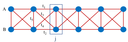
Figure 1: (Color online) The flat band Creutz lattice is given by $t_{1}=t_{2}^{*}=it$, $t_{3}=t_{4}=t$ and $t_{5}=0$. The flat band sawtooth lattice is given by $t_{1}=t_{4}=0$, $t_{2}=t$, $t_{3}=t_{5}=\sqrt{2}t$. The normal ladder is given by $t_{1}=t_{2}=t_{5}=t$ and $t_{3}=t_{4}=0$. The lower (upper) chain is the $\alpha=$B ($\alpha=$A) leg; the (black) rectangle shows the unit cell with lattice coordinate $j$.

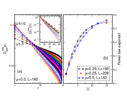
Figure 2: (Color online) DMRG results for the sawtooth lattice: (a) Pair Green function on the $B$ sublattice ($U=1,2,3,4,5,6,7,8,10,12,15$, $\rho=0.5$) exhibiting power law decay. The inset shows the exponential decay for the single particle Green function for the same cases. The thick (red) dashed line shows the analytically calculated $U\to 0$ limit giving a correlation length of $0.759$ lattice spacings (see text). (b) The exponents of the power law decay in (a) and also for the case of $\rho=0.25$.

Taking $t_{1}=it=t^{*}_{2}$, $t_{3}=t_{4}=t$, $t_{5}=0$, gives the Creutz lattice with two flat bands at energies Creutz (1999) $\pm 2t$, and a band gap of $4t$; taking $t_{1}=t_{4}=0$, $t_{2}=t$, $t_{5}=t_{3}=\sqrt{2}t$ gives the sawtooth latticeHuber and Altman (2010) with one flat band at $-2t$ and one dispersive band $\epsilon(k)=2t(1+{\rm cos}(k))$, and a band gap of $2t$, with the lattice momentum $k$ an integer multiple of $2\pi/L$ where $L$ is the number of unit cells. In what follows we make these flat band choices, our main goal being the study of pairing and the resulting superconducting phases. Since in the Hamiltonian, Eq.(1), the attractive interaction is of the contact on-site form, we expect on-site S-wave pairing to emerge, i.e. the maximum of the pair wavefunction corresponds to both $\uparrow$ and $\downarrow$ fermions being on the same site. Furthermore, the contact interaction implies that, in a mean-field approach, only on-site pairing terms are non-vanishing. A hallmark of pairing and pair transport is that the pair (single particle) Green function decays as a power (exponentially) with distance. These functions are given by,

$$G^{\alpha\beta}_{\sigma}(r) =\langle c^{\alpha}_{j+r\sigma}c^{\beta\dagger}_{j\sigma}\rangle,$$ (2)

$$G_{pair}^{\alpha\beta}(r) =\langle c^{\alpha}_{j+r\downarrow}c^{\alpha}_{j+r\uparrow}c^{\beta\dagger}_{j\uparrow}c^{\beta\dagger}_{j\downarrow}\rangle.$$ (3)

Another very important quantity characterizing the SC phase is the SC weight, $D_{s}$, defined in one dimension by W.Kohn (1964); Zotos et al. (1990); Shastry and Sutherland (1990); Scalapino et al. (1993); Hayward et al. (1995),

$$D_{s}\equiv\pi L\frac{d^{2}E_{GS}(\Phi)}{d\Phi^{2}}\bigg{|}_{\Phi=0}$$ (4)

where $E_{GS}(\Phi)$ is the ground-state energy in the presence of a phase twist $\Phi$ applied via the replacement $c_{j\sigma}^{\alpha}\to{\rm e}^{i\phi j}c_{j\sigma}^{\alpha}$ with $\phi=\Phi/L$. Since only near neighbor cells are connected, $H$ will depend on the phase gradient, $\phi$, which appears only in the hopping terms.

We use MF and the ALPS et al (2011) implementation of DMRG to calculate $E_{GS}(\Phi)$ on a lattice with periodic boundary conditions (PBC) which then yields $D_{s}$. Our PBC DMRG implementation is described in Ref.Mondaini et al. (2018), and allows us to reach up to $L=24$ unit cells. $G^{\alpha\beta}_{\sigma}(r)$ and $G_{pair}^{\alpha\beta}(r)$ are calculated with DMRG with open boundary conditions (OBC) where much larger sizes are achievable (up to $L=200$). When lattice sites are equivalent, the BCS MF starts with the usual substitution, $Uc^{\dagger}_{i\downarrow}c^{\dagger}_{i\uparrow}c^{\phantom{\dagger}}_{i\uparrow}c^{\phantom{\dagger}}_{i\downarrow}\rightarrow\Delta^{*}c^{\phantom{\dagger}}_{i\uparrow}c^{\phantom{\dagger}}_{i\downarrow}+c^{\dagger}_{i\downarrow}c^{\dagger}_{i\uparrow}\Delta-|\Delta|^{2}/U$. Here, $\Delta\equiv U\langle c^{\alpha}_{i\uparrow}c^{\alpha}_{i\downarrow}\rangle$ and $\langle c^{\alpha}_{i\uparrow}c^{\alpha}_{i\downarrow}\rangle$ is the site-independent order parameter, i.e. the wave function describing pair condensation. In general, it is complex but can be taken real when the lattice is uniform. However, when $U=0$, the eigenstate of $H$ on the sawtooth lattice shows that the density on a $B$ site is twice that on an $A$ site. This difference between $A$ and $B$ sites is expected to persist for $U\neq 0$ and, therefore, be also reflected in a difference between the order parameters on the two sublattices. Consequently, the mean field calculation should allow for distinct, unequal $\Delta^{A}$, $\Delta^{B}$, and for the local densities on $A$ and $B$ sites to be treated as variational parameters. Using a general quadratic trial Hamiltonian and applying the Gibbs-Bogoliubov inequality Kuzemsky (2015) (see Appendix A) we obtain the MF Hamiltonian,

$$H_{BCS} = \frac{LU}{2}+L\sum_{\alpha}\left[(|\Delta^{\alpha}|^{2}+\theta^{z2}_{\alpha})/U\right]$$ (5)

$$+\sum_{i,j,\alpha,\beta,\sigma}(t_{ij}c^{\alpha\dagger}_{i\sigma}c^{\beta\phantom{\dagger}}_{j\sigma}+H.c.)-\sum_{i,\alpha}(\mu+\frac{U}{2})n^{\alpha}_{i}$$

$$-\sum_{i,\alpha}\theta^{z}_{\alpha}(n^{\alpha}_{i\uparrow}+n^{\alpha}_{i\downarrow}-1)$$

$$-\sum_{i,\alpha}\left(\Delta^{\alpha*}c^{\alpha}_{i\uparrow}c^{\alpha}_{i\downarrow}+\Delta^{\alpha}c^{\alpha\dagger}_{i\downarrow}c^{\alpha\dagger}_{i\uparrow}\right),$$

where $\theta^{z}_{\alpha}\equiv U\langle n^{\alpha}_{\downarrow}+n^{\alpha}_{\uparrow}-1\rangle/2$. Fourier transforming, and defining the Nambu spinor $\Psi_{k}^{\dagger}\equiv(c^{\rm A\dagger}_{k\uparrow},c^{\rm B\dagger}_{k\uparrow},c^{\rm A\phantom{\dagger}}_{-k\downarrow},c^{\rm B\phantom{\dagger}}_{-k\downarrow})$, yields

$$H_{BCS}(\Phi) = \sum_{k}\Psi^{\dagger}_{k}{\cal M}_{k}(\phi)\Psi_{k}$$ (6)

$$+L\left(\frac{1}{U}\sum_{\alpha}(|\Delta^{\alpha}|^{2}+\theta_{\alpha}^{z2})-2\mu{-\frac{U}{2}}\right),$$

where ${\cal M}_{k}(\phi)$ is a $4\times 4$ Hermitian matrix (see Appendix A) and where we now display explicitly the phase twist $\Phi$ and its gradient $\phi$. It is clear that $\theta^{z}_{\alpha}$ is real but, in general, $\Delta^{\alpha}$ is complex. However, for lattices that are invariant under the $\text{A}\leftrightarrow\text{B}$ exchange, e.g. ladder and Creutz lattices, $\Delta$ is uniform and can be taken real for all $\Phi$. For a time-reversal symmetric Hamiltonian, $\Delta^{\alpha}$ can also be taken real and this is the case for the sawtooth lattice but only at $\Phi=0$. Finally, for lattices that are invariant under the $\text{A}\leftrightarrow\text{B}$ exchange, the mean-field parameters $\theta^{z}_{\alpha}$ also become homeogenous, i.e. independent of $\alpha$, such that they can be absorbed in the chemical potential $\mu$ leading back the usual simpler MF Hamiltonian.

Diagonalizing ${\cal M}_{k}(\phi)$ yields the ground state energy, $E_{GS}(\Phi)$, and allows us to solve the MF self-consistency equations giving $\Delta^{\alpha}$ and $\theta^{z}_{\alpha}$ and then obtain $D_{s}$. Apart from the additional MF parameters $\theta^{\alpha}$, our MF approach is the same as the one used to describe the usual BCS-BEC crossover, be it in lattices or in the bulk. However, the flat band dramatically changes the behavior and nature of the pairing at low interaction strength.

III Results and Discussion

The power and exponential decays of the pair and single particle Green functions on the Creutz and normal ladder lattices were presented in Ref.Mondaini et al. (2018). Here, we begin by establishing that the same behavior occurs in the sawtooth lattice. Figure 2(a) shows the pair Green functions along the $B$ sublattice of the sawtooth lattice for $U=1,2,3,4,5,6,7,8,10,12,15$ and $\rho=0.5$ exhibiting clear power law decay. The corresponding exponents, and also the exponents for the $\rho=0.25$ case, are shown in Fig.2(b). It is seen that the exponents behave similar to those for the Creutz latticeMondaini et al. (2018) where they take smaller values for smaller $U$, opposite to the behavior of the exponents on the normal ladderMondaini et al. (2018). The inset of Fig.2(a) shows the single particle Green functions for the same cases as in the main panel and exhibits exponential decay over many decades, even for small $U$. This establishes that, as in the usual BCS theory, the only transport in this system is via paired up and down fermions Grémaud and Batrouni (2021). However, for a flat band system, and in sharp contrast with the standard BCS situation, the length scale associated with the exponential decay of the single particle Green functions does not diverge (exponentially) as the interaction strength $U\rightarrow 0$. Instead it saturates to a finite value closely related to the exponential decay of the Wannier function of the flat band which is very fast. In addition, one can show that the pair wavefunction (not to be confused with the pair Green function) is also exponentially localized with a length scale of the same order as that of the single particle Green function. For instance, at $\rho=0.5$, one can show that both length scales have exactly the same value $0.759$ lattice spacings, in perfect agreement with the results in the inset of Fig.2(a). In other words, on conventional lattices, the spatial extent of the pair is exponentially large for small $U$ and decreases as $U$ increases, eventually becoming on-site pairing. In the flat band systems considered here, the pairing is essentially on-site for any value of $U$, even infinitesimal. Therefore, the physics of this system is different from that of the conventional BCS-BEC crossover.

In Ref.Mondaini et al. (2018), DMRG was used to calculate the SC weight, $D_{s}$, for the Creutz lattice and shown to be linear for small $U$, as predicted Peotta and Törmä (2015); Tovmasyan et al. (2016); Liang et al. (2017). Using our multi-band MF, Eq.(6), we calculate $E_{GS}(\Phi)$ (see Appendix A) and then $D_{s}$, Eq.(4), for the same parameters in Ref.Mondaini et al. (2018). We compare the MF and DMRG results in Fig.3. Figure 3(a) shows clearly that the MF results are remarkably accurate for a very wide range of $U$ values at the two densities studied. The dashed lines in Fig.3(a) are given by $D_{s}=\pi U\rho(1-\rho)$ derived from the results of Ref.Tovmasyan et al. (2016) where it was assumed that $U$ is much smaller than the gap between the bands. Consequently, at these small values of $U$, the physics is dominated by the flat band, and the states can be projected on it (see Appendix B). This means that the upper band does not contribute to the physics in this limit. With the added assumption that $\Delta$ is uniform and independent of the applied phase twist, it was shownTovmasyan et al. (2016) that for such very small values of the coupling, $D_{s}$ is linear in $U$ and is proportional to the quantum metricPeotta and Törmä (2015), Eq.(47). It is to be emphasized that these approximations are valid only for $U$ much smaller than the gap between the bands and, therefore, the physics at very low $U$ is dominated by the flat bandTovmasyan et al. (2016) and the topological properties of the lattice. The physics at intermediate $U$ (of the order of the interband gap) is dominated by very strong mixing between the two bands, with both bands contributing significantly to the properties of the system, such as $D_{s}$. At very strong $U$, the physics is that of hard core bosons governed by a dispersive Hamiltonian with near neighbor repulsionEmery (1976); Micnas et al. (1990). It is remarkable that our multi-band MF calculation agrees with DMRG over such a wide range of parameters despite the marked difference in mechanism.

It is evident that the agreement between our MF and DMRG is better for the lower density, $\rho=0.25$. Figure 3(b) emphasizes the dependence of the MF accuracy on the interplay of $U$ and $\rho$. For $U=t$, MF gives a very good description for all fillings up to half filling, $\rho=1$. For $U=8t$, MF is accurate only up to around $\rho=0.5$. In particular, at half filling, $\rho=1$, the system should be a band insulator (the lower band is full) but MF at $U=8t$ yields a finite $D_{s}$.

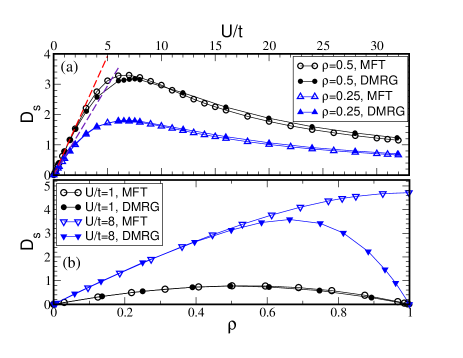
Figure 3: (Color online) Creutz lattice: (a) SC weight, $D_{s}$, vs. $U/t$ comparing BCS MF with DMRGMondaini et al. (2018). Very good agreement is seen over a wide range of values. Dashed lines are the linear predictions Tovmasyan et al. (2016) for very small $U$ (see text). (b) BCS MF agrees very well with DMRG over a wider range of $\rho$ for low $U$. For large $U$, the agreement is good at low densities. DMRG calculations were done on $L=16$ lattice with PBC.

With this agreement between MF and DMRG for the Creutz lattice, we now study $D_{s}$ on the sawtooth lattice. We perform exact DMRG calculations for the sawtooth lattice with PBC and sizes up to $L=24$ to calculate $D_{s}$ and compare with our extended BCS MF. Figure 4 shows $D_{s}$ vs. $U/t$ for two densities, $\rho=0.5,\,0.25$. Similar to the Creutz, $D_{s}$ also increases linearly at first, reaches a maximum and then decreases slowly. Figure 4 also shows that our multi-band MF values agree very well with DMRG over the entire range of $U$ values we explored. We emphasize that without the additional MF parameters $\theta^{z}_{\alpha}$, agreement between MF and DMRG would be quite poor for $D_{s}$ already at values of $U\approx 5t$ (see Appendix A). We note that the values of $D_{s}$ for sawtooth are more than a factor of $2$ smaller than the corresponding values for Creutz. The Creutz lattice offers a higher superfluid density for the same particle density. Furthermore, the low $U$ behavior of $D_{s}$ is linear in $U$, and the dashed lines in Fig.4 are fits to the low $U$ linear parts of the curves; the slope for $\rho=0.5(0.25)$ is $0.401(0.303)$. Using the results of Ref.Tovmasyan et al. (2016), which predict a slope proportional to the quantum metric, $\mathcal{Q}=\frac{2}{3\sqrt{3}}$, we find slopes of $0.6$ and $0.45$ for $\rho=0.5$ and $0.25$ respectively which do not agree with the exact numerical values like they did for the Creutz lattice. This disagreement is due to the fact that the $A$ and $B$ sublattices are not equivalent in the sawtooth case: $\Delta^{A}\neq\Delta^{B}$ and $\rho^{A}\neq\rho^{B}$, and, consequently, the assumptions in Refs.Tovmasyan et al. (2016); Peotta and Törmä (2015) which led to $D_{s}$ being proportional to the quantum metric are no longer valid. In fact, the derivation in Ref.Peotta and Törmä (2015) not only assumes that, for all values of the phase gradient $\phi$, $\Delta$ is the same for all sites, but also that it has a vanishing first derivative with respect to $\phi$, at $\phi=0$. It turns out that the latter assumption is, in general, not valid as soon as $\Delta$ becomes sub-lattice dependent, since the $U(1)$ symmetry only allows one to fix the global phase of the mean-field parameters, leaving the possibility of a $\phi$ dependent relative phase between the $\Delta^{\alpha}$. We found that when $\phi\neq 0$, the phase difference between $\Delta^{A}$ and $\Delta^{B}$ for the sawtooth lattice is exactly equal to the phase gradient $\phi$. Nonetheless, by projecting carefully on the flat band without making the above-mentioned simplifying assumptions, we generalized the mean field computation of the slope of the superfluid weight, see Appendix B, as a function of the total density $\rho$. The results are displayed in Fig. 5, where we compare our analytical results for the slope at small $U$ with our full band computation and also to what one obtains by using the results of Ref. Peotta and Törmä (2015). In addition we show the results from our DMRG calculation. As can be seen clearly, the agreement between all our approaches is excellent, but not with the results predicted in Ref. Peotta and Törmä (2015), which only include the quantum metric. In particular, our projection method gives the slope of $D_{s}$ at $\rho=0.5$ ($\rho=0.25$) to be $0.407$ ($0.311$) which compares very well with the DMRG results $0.401$ ($0.303$).

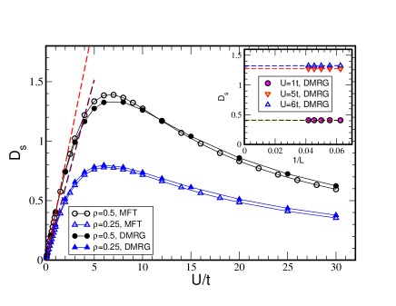
Figure 4: (Color online) SC weight, $D_{s}$, for the sawtooth lattice comparing MF with DMRG ($L=16$) showing excellent agreement. Dashed lines are linear fits at low $U$ where $D_{s}$ is predicted to be linear in $U$. See text for a discussion of the slopes. The inset shows $D_{s}$ vs $L^{-1}$ at $U=1,\,2,\,3$ for $\rho=0.5$ and illustrates that finite size effects are very small.

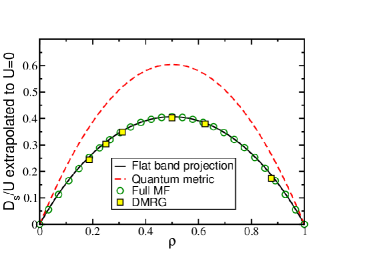
Figure 5: (Color online) Sawtooth lattice: SC weight $D_{s}/U$ extrapolated to $U=0$ as a function of the total density $\rho$ from the projection onto the flat band (black continuous line), compared with the full band computations (green circles) and with the results of ref. Peotta and Törmä (2015), which only include the quantum metric term (red dashed line). The yellow squares are the exact results obtained with DMRG.

We elucidate further the agreement between our MF and exact DMRG results by comparing the order parameter $\Delta^{\alpha}/U$ given by the two methods. With MF, we calculate directly $\Delta^{\alpha}/U=\langle c^{\alpha}_{i\uparrow}c^{\alpha}_{i\downarrow}\rangle$; with DMRG, we use $\Delta^{\alpha*}\Delta^{\alpha}=\langle c^{\alpha\dagger}_{i\downarrow}c^{\alpha\dagger}_{i\uparrow}c^{\alpha\phantom{\dagger}}_{i\uparrow}c^{\alpha\phantom{\dagger}}_{i\downarrow}\rangle-\langle n^{\alpha}_{i\uparrow}\rangle\langle n^{\alpha}_{i\downarrow}\rangle$. We show in Fig.6 the MF and DMRG values for the Creutz system and MF values for the normal ladder where for these systems $\Delta^{A}=\Delta^{B}=\Delta$. Note that for the normal ladder $\Delta/U$ vanishes exponentially as $U\to 0$ making accurate DMRG determination not feasible because it requires exponentially large systems. On the other hand, for the Creutz system $\Delta(U\to 0)/U$ is finite even though $\Delta(U=0)=0$: Here, even for infinitesimal attraction, the pairing parameter $\Delta/U$ acquires a large finite value. We see in Fig.6 excellent agreement between the MF and DMRG values of $\Delta/U$ for a very wide range of $U$ values. The difference in behavior of $\Delta/U$ between normal ladder and Creutz lattices can be understood as follows: For a dispersive band, it is well known that in the small $U/t$ limit, pairing only occurs at the Fermi level and involves an (exponentially) small fraction of the free fermions. Consequently, the pair density itself becomes (exponentially) small. Furthermore, for small $U$, the correlation between the paired electrons (the pair size) extends over a very large distance. In contrast, there is no Fermi surface for a flat band, and fermions at all momenta can form pairs leading to a sizeable contribution to the pair density and yielding a finite value even for arbitrarily small $U$. Additionally, even for infinitesimal $U$, the system is strongly correlated because $U$ is much larger than the width of the flat band. In this case, the pair size is essentially on-site even for very small $U$. We emphasize that, even though the order parameter does not vanish at small $U$, the superfluid weight, $D_{s}$, and the charge gap (both controlled by $\Delta^{\alpha}$) do vanish (linearly) with $U$.

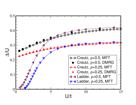
Figure 6: (Color online) The MF pairing parameter, $\Delta/U$, as a function of $U/t$ for the Creutz and normal ladder lattices. Agreement between DMRG and MF is excellent.

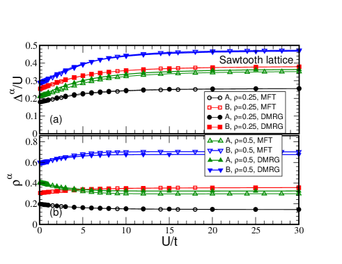
Figure 7: (Color online) Sawtooth lattice: (a) The MF pairing parameter, $\Delta^{\alpha}/U$, as a function of $U/t$; (b) $\rho^{\alpha}$ vs $U/t$.

The sawtooth lattice MF and DMRG results are shown in Fig.7. Figure 7(a) shows $\Delta^{\alpha}/U$ as a function of $U/t$ for two densities, $\rho=0.5$ and $0.25$. We see that the behavior as $U\to 0$ is qualitatively similar to that of the Creutz lattice. However, here we observe the imperative difference that, for the whole range of $U$, $\Delta^{A}\neq\Delta^{B}$, and that our MF results are in excellent agreement with DMRG. Furthermore, we see a similar pattern between $\rho^{A}$ and $\rho^{B}$ in Fig.7(b): for all $U$, their values remain clearly different. These striking differences between the $A$ and $B$ sublattices cannot be obtained accurately with a simple BCS MF calculation, which, at large $U$, inevitably leads to $\Delta^{A}=\Delta^{B}$ and thereby in $\rho^{A}=\rho^{B}$ (see Appendix A). To obtain correct behavior, we stress the importance of treating the local densities as variational MF parameters.

IV Conclusions

Using mean field and exact DMRG calculations, we studied the pairing and superconducting properties of the attractive fermionic Hubbard model in two flat band lattices with non-trivial winding numbers, the Creutz and sawtooth lattices. The difference, however, is that only the Creutz lattice is genuinely topological owing to a chiral (sub-lattice) symmetry, resulting in a quantized winding number and zero energy edge modes for open boundary conditions. On the contrary, the lack of sublattice symmetry for the sawtooth lattice not only results in a non-quantized winding number, but also causes the densities and pairing parameters on the two sublattices to be different and necessitates the use of a mean field method where the local densities and pairing parameters are all MF parameters, as we showed here. While mean field calculations may be expected to give reasonably accurate results for weak coupling and low densities, we show that our mean field describes the system remarkably well for a very wide range of coupling values and densities. It only fails when both the density and coupling attain high values, Fig.3(b). We emphasize one of our main results: since $\Delta^{A}\neq\Delta^{B}$ for sawtooth, the superconducting weight, $D_{s}$, is no longer simply proportional to the quantum metric for low $U$ values, but is still linear in $U$. We calculated here the correct and more general linear behavior (Appendix B). This is expected to hold for any topological lattice where sublattices are not equivalent. Finally, beyond static properties, our results emphasize that for lattices with inequivalent sites, it is crucial to use the extended mean field approach for time-dependent situations, such as AC or DC Josephson effects Pyykkönen et al. (2021).

Acknowledgments: S.M.C. is supported by a National University of Singapore President’s Graduate Fellowship. The DMRG computations were performed with the resources of the National Supercomputing Centre, Singapore (www.nscc.sg). This research is supported by the National Research Foundation, Prime Minister’s Office and the Ministry of Education (Singapore) under the Research Centres of Excellence programme.

Appendix A Multi-band mean field method

The DMRG method we used for the exact calculation of $D_{s}$, and the implementation of the periodic boundary condition are discussed in Ref.Mondaini et al. (2018). Here we discuss in some more detail the multi-band MF method we use in this work.

We start with a general quadratic trial Hamiltonian,

$$H_{trial} = \sum_{i,j,\alpha,\beta,\sigma}(t_{ij}c^{\alpha\dagger}_{i\sigma}c^{\beta\phantom{\dagger}}_{j\sigma}+H.c.)-\mu\sum_{i,\alpha}n^{\alpha}_{i}$$ (7)

$$-\sum_{i,\alpha}\left(\theta^{\alpha}_{\downarrow}n^{\alpha}_{i\uparrow}+\theta^{\alpha}_{\uparrow}n^{\alpha}_{i\downarrow}\right)$$

$$-\sum_{i,\alpha}\left(\Delta^{\alpha*}c^{\alpha}_{i\uparrow}c^{\alpha}_{i\downarrow}+\Delta^{\alpha}c^{\alpha\dagger}_{i\downarrow}c^{\alpha\dagger}_{i\uparrow}\right),$$

where $\theta^{\alpha}_{\sigma}$ and $\Delta^{\alpha}$ are the variational MF parameters to be determined. The Gibbs-Bogoliubov inequalityKuzemsky (2015) gives an upper bound on the true free energy, $F$, of the model governed by the Hamiltonian Eq.(1),

$$F\leq{\rm Tr}[HW_{trial}]+\frac{1}{\beta}{\rm Tr}[W_{trial}{\rm ln}W_{trial}],$$ (8)

where the trial Boltzmann weight is given by,

$$W_{trial}=\frac{1}{Z_{trial}}{\rm e}^{-\beta H_{trial}},$$ (9)

and $Z_{trial}={\rm Tr\,}{\rm e}^{-\beta H_{trial}}={\rm e}^{-\beta F_{trial}}$. Substituting $W_{trial}$ in Eq.(8) and using Wick’s theorm, we get,

$$F \leq -U\sum_{i,\alpha}\left(\langle n^{\alpha}_{i\uparrow}\rangle\langle n^{\alpha}_{i\downarrow}\rangle+\langle c^{\alpha\dagger}_{i\downarrow}c^{\alpha\dagger}_{i\uparrow}\rangle\langle c^{\alpha\phantom{\dagger}}_{i\uparrow}c^{\alpha\phantom{\dagger}}_{i\downarrow}\rangle\right)$$

$$+\sum_{i,\alpha}\left(\theta^{\alpha}_{\downarrow}\langle n^{\alpha}_{i\uparrow}\rangle+\theta^{\alpha}_{\uparrow}\langle n^{\alpha}_{i\downarrow}\rangle\right)$$

$$+\sum_{i,\alpha}\left(\Delta^{\alpha*}\langle c^{\alpha}_{i\uparrow}c^{\alpha}_{i\downarrow}\rangle+\Delta^{\alpha}\langle c^{\alpha\dagger}_{i\downarrow}c^{\alpha\dagger}_{i\uparrow}\rangle\right)+F_{trial}.$$

We minimize the right hand side with respect to the variational parameters and obtain,

$$\theta^{\alpha}_{\uparrow}=U\langle n^{\alpha}_{i\uparrow}\rangle,\,\,\,\theta^{\alpha}_{\downarrow}=U\langle n^{\alpha}_{i\downarrow}\rangle,\,\,\,\,\Delta^{\alpha}=U\langle c^{\alpha}_{i\uparrow}c^{\alpha}_{i\downarrow}\rangle.$$ (11)

We substitute these expressions in Eq.(8) to obtain the optimized free energy,

$$F \leq \frac{1}{U}\sum_{i,\alpha}(\theta^{\alpha}_{\downarrow}\theta^{\alpha}_{\uparrow}+|\Delta^{\alpha}|^{2})-\frac{1}{\beta}{\rm ln\,Tr}\,{\rm e}^{-\beta H_{trial}}$$ (12)

$$\leq -\frac{1}{\beta}{\rm\ln\,Tr}\,{\rm e}^{-\beta\left(\frac{1}{U}\sum_{i,\alpha}(\theta^{\alpha}_{\downarrow}\theta^{\alpha}_{\uparrow}+|\Delta^{\alpha}|^{2})+H_{trial}\right)}$$

$$\equiv -\frac{1}{\beta}{\rm\ln\,Tr}\,{\rm e}^{-\beta H_{BCS}},$$

which defines $H_{BCS}$. Since we are dealing with systems with balanced up and down populations, $\theta^{\alpha}_{\uparrow}=\theta^{\alpha}_{\downarrow}$, we can instead define $\theta^{z}_{\alpha}\equiv(\theta^{\alpha}_{\uparrow}+\theta^{\alpha}_{\downarrow}-U)/2$. This allows us to rewrite,

$$H_{BCS} = \frac{LU}{2}+L\sum_{\alpha}\left[(|\Delta^{\alpha}|^{2}+\theta^{z2}_{\alpha})/U\right]$$ (13)

$$+\sum_{i,j,\alpha,\beta,\sigma}(t_{ij}c^{\alpha\dagger}_{i\sigma}c^{\beta\phantom{\dagger}}_{j\sigma}+H.c.)-\sum_{i,\alpha}(\mu+\frac{U}{2})n^{\alpha}_{i}$$

$$-\sum_{i,\alpha}\left(\theta^{z}_{\alpha}(n^{\alpha}_{i\uparrow}+n^{\alpha}_{i\downarrow}-1\right)$$

$$-\sum_{i,\alpha}\left(\Delta^{\alpha*}c^{\alpha}_{i\uparrow}c^{\alpha}_{i\downarrow}+\Delta^{\alpha}c^{\alpha\dagger}_{i\downarrow}c^{\alpha\dagger}_{i\uparrow}\right),$$

which is Eq.(5). This can now be put in momentum space via the Fourier transform,

$$\chi_{r\sigma}=\frac{1}{\sqrt{L}}\sum_{k}{\rm e}^{irk}{\tilde{\chi}}_{k\sigma},$$ (14)

where $k=2\pi n/L$ ($n=-L/2+1,\dots,0,1,\dots,L/2$) and $\chi^{\dagger}_{r\sigma}\equiv(c^{A\dagger}_{r\sigma}\,\,c^{B\dagger}_{r\sigma})$. Defining the 4-component Nambu spinor $\Psi^{\dagger}_{k}\equiv(c^{\rm A\dagger}_{k\uparrow},c^{\rm B\dagger}_{k\uparrow},c^{\rm A\phantom{\dagger}}_{-k\downarrow},c^{\rm B\phantom{\dagger}}_{-k\downarrow})$, and with the phase gradient given by $\phi=\Phi/L$, we obtain

$$H_{BCS}(\Phi) = \sum_{k}\Psi^{\dagger}_{k}{\cal M}_{k}(\phi)\Psi_{k}$$

$$+L\left(\frac{1}{U}\sum_{\alpha}(|\Delta^{\alpha}|^{2}+\theta^{z\,2}_{\alpha})-2\mu-\frac{U}{2}\right),$$

which is Eq.(6). For the general chain depicted in Fig.1, the matrix ${\cal M}_{k}(\phi)$ is

$${\cal M}_{k}(\phi)=\begin{pmatrix}{\cal K}(\phi+k)&{\cal D}\\ {\cal D}^{*}&-{\cal K}^{T}(\phi-k)\end{pmatrix},$$ (16)

where,

$${\cal K}(\phi+k)=\begin{pmatrix}{\cal K}_{11}-{\bar{\mu}}^{A}&&&{\cal K}_{21}\\ {\cal K}_{12}&&&{\cal K}_{22}-{\bar{\mu}}^{B}\end{pmatrix},$$ (17)

with $\bar{\mu}^{\alpha}=\mu+U/2+\theta^{z}_{\alpha}$, ${\cal K}_{11}=t_{1}{\rm e}^{i(\phi+k)}+t_{1}^{*}{\rm e}^{-i(\phi+k)}$, ${\cal K}_{22}=t_{2}{\rm e}^{i(\phi+k)}+t_{2}^{*}{\rm e}^{-i(\phi+k)}$, ${\cal K}_{12}={\cal K}_{21}^{*}=t_{5}+t_{3}{\rm e}^{i(\phi+k)}+t_{4}{\rm e}^{-i(\phi+k)}$. The matrix ${\cal D}$ is given by,

$${\cal D}=\begin{pmatrix}\Delta^{A}&0\\ 0&\Delta^{B}\end{pmatrix},$$ (18)

The three models we address here are obtained by appropriate choices of the hopping parameters. The normal ladder is given by $t_{3}=t_{4}=0,\,t_{1}=t_{2}=t_{5}=t$; the flat band Creutz model by $t_{1}=t_{2}^{*}=it$, $t_{3}=t_{4}=t$, $t_{5}=0$; and the sawtooth model by $t_{1}=t_{4}=0$, $t_{2}=t$, $t_{5}=t_{3}=\sqrt{2}t$.

${\cal M}_{k}(\phi)$ can be diagonalized giving the ground state energy, $E_{GS}(\Phi)$,

$$E_{GS}(\phi) = L\left(\frac{1}{U}\sum_{\alpha}(|\Delta^{\alpha}|^{2}+\theta^{z\,2}_{\alpha})-2\mu-\frac{U}{2}\right)$$ (19)

$$+\displaystyle\sum_{k}\left(\lambda_{1}(k,\phi)+\lambda_{2}(k,\phi)\right),$$

where $\lambda_{1,2}$ are the negative eigenvalues. The mean field parameters are obtained by minimizing $E_{GS}(\phi)$ with respect to those parameters or, equivalently, by solving the self consistency equations,

$$\Delta^{\alpha}=U\langle c^{\alpha}_{i\uparrow}c^{\alpha}_{i\downarrow}\rangle,\hskip 28.45274pt\theta^{z}_{\alpha}=U(\langle n^{\alpha}_{i}\rangle-1)/2,$$ (20)

with $n^{\alpha}_{i}=c^{\alpha\dagger}_{i\uparrow}c^{\alpha\phantom{\dagger}}_{i\uparrow}+c^{\alpha\dagger}_{i\downarrow}c^{\alpha\phantom{\dagger}}_{i\downarrow}$.

For the normal ladder and Creutz models, $\Delta^{A}=\Delta^{B}$ and $\rho^{A}=\rho^{B}$, so that we can use the simple BCS MF with a single variational parameter, $\Delta$, which is uniform on all sites. The eigenvalues of ${\cal M}_{k}(\phi)$ can then be obtained in closed form. In these cases, the results of the simple BCS MF and the more extended MF we use here are identical. However, for the sawtooth lattice with its unequal $A$ and $B$ sites, the two mean field methods are not equivalent and only the extended method we presented here gives correct results, especially at strong coupling.

If, instead of using the extended MF method, we use the simple BCS mean field where only the $\Delta^{\alpha}$ are MF variational parameters, $Uc^{\alpha\dagger}_{i\downarrow}c^{\alpha\dagger}_{i\uparrow}c^{\alpha\phantom{\dagger}}_{i\uparrow}c^{\alpha\phantom{\dagger}}_{i\downarrow}\rightarrow\Delta^{\alpha*}c^{\alpha\phantom{\dagger}}_{i\uparrow}c^{\alpha\phantom{\dagger}}_{i\downarrow}+c^{\alpha\dagger}_{i\downarrow}c^{\alpha\dagger}_{i\uparrow}\Delta^{\alpha}-|\Delta^{\alpha}|^{2}/U$, we obtain reasonable results only for low $U$ but quantitatively incorrect results as $U$ increases.

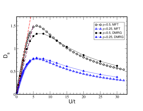
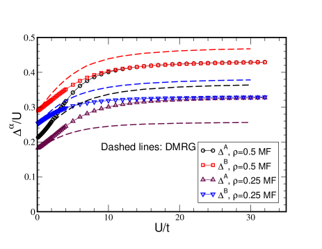
Figure 8: (Color online) Sawtooth lattice. Top panel: $D_{s}$ versus $U/t$ using the simple BCS MF substitution. We find a quite good agreement with DMRG for small $U$, but a relatively poor one at large U. Bottom panel: The pairing parameter, $\Delta^{\alpha}$, versus $U/t$. Excellent agreement with DMRG for small $U$. As $U$ increases, the simple MF results become quantitatively incorrect: $\Delta^{A}\to\Delta^{B}$ which is not what exact DMRG results show. DMRG shows that $\Delta^{A}$ and $\Delta^{B}$ remain unequal.

The top panel of Fig.8 shows for the sawtooth lattice $D_{s}$ versus $U/t$ using the simple BCS MF calculation. We see that at low $U$, agreement with DMRG is still excellent but for medium and large values of $U$ the agreement not as good. Compare with Fig. 3 in the main text. The bottom panel shows, for the same system, the pairing parameters, $\Delta^{A}/U$ and $\Delta^{B}/U$ versus $U/t$ and, again, exhibits good agreement with DMRG for low values of $U$. However, as $U$ increases, the behavior of $\Delta^{\alpha}$ becomes qualitatively and quantitatively incorrect: The simple MF shows that, at large $U$, $\Delta^{A}=\Delta^{B}$, which the exact DMRG results show never happens (compare with Fig. 7(a)). The same behavior is observed for $\rho^{A}$ and $\rho^{B}$ (not shown). It is therefore crucial to use the correct mean field decoupling in order to obtain qualitatively correct (and quantitatively accurate) results.

Appendix B Superfluid weight for a flat band system with inequivalent sites

B.1 General situation

In a mean-field approach, the superfluid weight reads:

$$D_{s}=\pi\left.\frac{d^{2}\epsilon_{GS}\left(\Delta^{\alpha}(\phi),\Delta^{\alpha*}(\phi),\phi\right)}{d^{2}\phi}\right|_{\phi=0}$$ (21)

where, $\phi$ is the phase gradient and, $\epsilon_{GS}=E_{GS}/L$ is the ground state energy per unit cell, see Eq. (19),

$$\epsilon_{GS}(\Delta^{\alpha},\Delta^{\alpha*},\phi)=\frac{1}{U}\sum_{\alpha}|\Delta^{\alpha}|^{2}+\frac{1}{L}\sum_{k,n}\lambda_{n}(k,\Delta^{\alpha},\Delta^{\alpha*},\phi),$$ (22)

where we have made explicit the dependence on $\Delta^{\alpha}$. For simplification, we have omitted (i) the $\theta^{\alpha}$ terms which do not play an important role at low $U$, and (ii) the explicit dependence on the chemical potential $\mu$ since, even for inequivalent sites, it does not give any additional contribution to $D_{s}$.

Differentiating $\epsilon_{GS}$ twice with respect to $\phi$, and using the fact that we have $\frac{\partial\epsilon_{GS}}{\partial\Delta^{\alpha}}=\frac{\partial\epsilon_{GS}}{\partial\Delta^{\alpha*}}=0$ along the mean-field solution, $\Delta^{\alpha}=\Delta_{mf}^{\alpha}(\phi)$, one obtains

$$\frac{D_{s}}{\pi}=\frac{1}{L}\sum_{k,n} \left(\frac{\partial^{2}\lambda_{n}}{\partial\phi^{2}}+\sum_{\alpha}\frac{\partial^{2}\lambda_{n}}{\partial\Delta^{\alpha}\partial\phi}\frac{d\Delta_{mf}^{\alpha}}{d\phi}\right.$$ (23)

$$\left.+\sum_{\alpha}\frac{\partial^{2}\lambda_{n}}{\partial\Delta^{\alpha*}\partial\phi}\frac{d\Delta_{mf}^{\alpha*}}{d\phi}\right),$$ (24)

where all derivatives are computed at $\phi=0$ and $\Delta^{\alpha}=\Delta_{mf}^{\alpha}(\phi=0)$. For systems which are invariant under the time-reversal symmetry, and with equivalent sites, the $U(1)$ symmetry allows us to have all $\Delta^{\alpha*}$ to be real, so that $\frac{d\Delta_{mf}^{\alpha*}}{d\phi}=0$ at $\phi=0$. In this situation, the only contribution to $D_{s}$ is the first term which, in the $U\rightarrow 0$ limit, can be shown to be proportional to the quantum metric Peotta and Törmä (2015).

Generally, in the $U\rightarrow 0$ limit and projecting on the flat band, one can approximate the chemical potential by $\mu\approx\epsilon_{FB}+aU$, and the mean field parameters by $\Delta^{\alpha}\approx U\tilde{\Delta}^{\alpha}$, thereby allowing us to factor out the $U$ dependence of the ground state energy:

$$\epsilon_{GS}(\tilde{\Delta}^{\alpha},\tilde{\Delta}^{\alpha*},\phi) =-\frac{U}{L}\sum_{k}d_{k}(\tilde{\Delta}^{\alpha},\tilde{\Delta}^{\alpha*},\phi)$$ (25)

with

$$d_{k}(\tilde{\Delta}^{\alpha},\tilde{\Delta}^{\alpha*},\phi) =\sqrt{a^{2}+|\tilde{b}_{k}(\tilde{\Delta}^{\alpha},\phi)|^{2}}$$ (26)

$$\tilde{b}_{k}(\tilde{\Delta}^{\alpha},\phi) =\sum_{\alpha}P^{*}_{\alpha}(-k+\phi)\tilde{\Delta}^{\alpha}P^{*}_{\alpha}(k+\phi),$$ (27)

where $P_{\alpha}(k)$ are the site components of the Bloch vector of the flat band, i.e. the eigenvector of the matrix $\mathcal{K}(k)$. The mean-field parameters and $a$ fulfill the following self-consistent equations:

$$\rho =\frac{1}{2}+\frac{a}{2L}\sum_{k}\frac{1}{d_{k}(\tilde{\Delta}^{\alpha},\tilde{\Delta}^{\alpha*},\phi)}$$ (28)

$$\tilde{\Delta}^{\alpha} =\frac{1}{2L}\sum_{k}\frac{P_{\alpha}(-k+\phi)P_{\alpha}(k+\phi)\tilde{b}_{k}(\tilde{\Delta}^{\alpha},\phi)}{d_{k}(\tilde{\Delta}^{\alpha},\tilde{\Delta}^{\alpha*},\phi)},$$ (29)

and the superfluid weight reads:

$$D_{s}=-U\pi \left(\frac{1}{L}\sum_{k}\left.\frac{\partial^{2}d_{k}}{\partial\phi^{2}}\right|_{\tilde{\Delta}_{mf}^{\alpha}(0),\phi=0}\right.$$ (30)

$$+\frac{1}{L}\sum_{k}\sum_{\alpha}\left.\frac{\partial^{2}d_{k}}{\partial\phi\partial\tilde{\Delta}^{\alpha}}\right|_{\tilde{\Delta}_{mf}^{\alpha}(0),\phi=0}\left.\frac{d\tilde{\Delta}_{mf}^{\alpha}}{d\phi}\right|_{\phi=0}$$

$$+\left.\frac{1}{L}\sum_{k}\sum_{\alpha}\left.\frac{\partial^{2}d_{k}}{\partial\phi\partial\tilde{\Delta}^{\alpha*}}\right|_{\tilde{\Delta}_{mf}^{\alpha}(0),\phi=0}\left.\frac{d\tilde{\Delta}_{mf}^{\alpha*}}{d\phi}\right|_{\phi=0}\right).$$

Differentiating the self-consistent equation (29) with respect to $\phi$ allows us to find a set of coupled linear equations fulfilled by all $\left.\frac{d\tilde{\Delta}^{\alpha}_{mf}}{d\phi}\right|_{\phi=0}$. For time-reversal invariant system, we can show that all these quantities are purely imaginary, and the set of linear equations reads formally $O_{\alpha\alpha^{\prime}}X_{\alpha^{\prime}}=Y_{\alpha}$, with $X_{\alpha}=\left.\frac{d\tilde{\Delta}^{\alpha}_{mf}}{d\phi}\right|_{\phi=0}$ and

$$O_{\alpha\alpha^{\prime}} =\delta_{\alpha\alpha^{\prime}}-\frac{1}{2L}\sum_{k}\frac{P_{\alpha}(k)P^{*}_{\alpha}(k)P_{\alpha^{\prime}}(k)P^{*}_{\alpha^{\prime}}(k)}{d_{k}}$$ (31)

$$Y_{\alpha} =\frac{1}{2L}\sum_{k}\frac{b_{k}}{d_{k}}\left(P^{*}_{\alpha}(k)\partial_{k}P_{\alpha}(k)-\partial_{k}P^{*}_{\alpha}(k)P_{\alpha}(k)\right)$$

$$+\frac{1}{2L}\sum_{k}\frac{P_{\alpha}(k)P^{*}_{\alpha}(k)}{d_{k}}\partial_{\phi}b_{k}.$$ (32)

Note that the matrix $O$ is singular. Indeed, one can see that for $X_{\alpha}=\tilde{\Delta}_{mf}^{\alpha}$ at $\phi=0$, the self-consistent equations lead to $\sum_{\alpha^{\prime}}O_{\alpha\alpha^{\prime}}\tilde{\Delta}_{mf}^{\alpha}=0$, which is just the $U(1)$ symmetry: if one adds a global phase to all MF parameters, it does not change the GS, i.e. the self-consistent equations are still fulfilled.

B.2 Two-band lattices

In the specific case of a two-band system, like the sawtooth lattice, the $2\times 2$ matrix $\mathcal{K}(k)$ can be written formally as follows,

$$\mathcal{K}(k) =e_{0}(k)\openone+\vec{e}(k)\cdot\vec{\sigma}$$

$$\vec{e}(k) =|e(k)|\left(\sin{\vartheta_{k}}\cos{\varphi_{k}},\sin{\vartheta_{k}}\sin{\varphi_{k}},\cos{\vartheta_{k}}\right),$$ (33)

where ${\vec{\sigma}}$ are the Pauli matrices. Assuming that the flat band corresponds to the lower band, the Bloch eigenvector reads

$$P_{A}(k)=-\sin{\frac{\vartheta_{k}}{2}}e^{-i\varphi_{k}/2}\qquad P_{B}(k)=\cos{\frac{\vartheta_{k}}{2}}e^{i\varphi_{k}/2}.$$ (34)

Let us introduce the notations:

$$\tilde{\Delta}^{A}=\tilde{\Delta}(1-\delta)\text{ and }\tilde{\Delta}^{B}=\tilde{\Delta}(1+\delta),$$ (35)

and, using Eqs.(26,27), we find at $\phi=0$

$$\tilde{b}_{k} =\tilde{\Delta}\biggl{(}1+\delta\cos{\vartheta_{k}}\biggr{)}$$ (36)

$$d_{k} =\sqrt{a^{2}+\tilde{\Delta}^{2}\left(1+\delta\cos{\vartheta_{k}}\right)^{2}}$$ (37)

fulfilling the following equations:

$$\rho-\frac{1}{2} =\frac{a}{2L}\sum_{k}\frac{1}{d_{k}}$$ (38)

$$1 =\frac{1}{4L}\sum_{k}\frac{1+\delta\cos{\vartheta_{k}}}{d_{k}}$$ (39)

$$\delta =\frac{1}{4L}\sum_{k}\frac{\cos{\vartheta_{k}}\left(1+\delta\cos{\vartheta_{k}}\right)}{d_{k}}$$ (40)

After some straighforward computations, one can show that the superfluid weight reads:

$$D_{s}=U\tilde{\Delta}^{2}\Biggl{(} \frac{2\pi}{L}\sum_{k}\frac{\mathcal{B}_{k}}{d_{k}}$$

$$+ \delta\frac{2\pi}{L}\sum_{k}\frac{\left(\sin{\vartheta_{k}}\partial^{2}_{k}\vartheta_{k}+\cos{\vartheta_{k}}(\partial_{k}\vartheta_{k})^{2}\right)}{2d_{k}}$$

$$+ \delta^{2}\frac{2\pi}{L}\sum_{k}\frac{\left(\sin{\vartheta_{k}}\cos{\vartheta_{k}}\partial^{2}_{k}\vartheta_{k}-\sin^{2}{\vartheta_{k}}(\partial_{k}\varphi_{k})^{2}\right)}{2d_{k}}$$

$$+\gamma(1-\delta^{2})\frac{2\pi}{L}\sum_{k}\frac{(1-\cos^{2}{\vartheta_{k}})\partial_{k}\varphi_{k}}{2d_{k}}\Biggr{)},$$ (41)

where

$$\mathcal{B}_{k} =2\sum_{\alpha}\partial_{k}P^{*}_{\alpha}\partial_{k}P_{\alpha}-2|\sum_{\alpha}\partial_{k}P^{*}_{\alpha}P_{\alpha}|^{2}$$

$$=\frac{1}{2}\left((\partial_{k}\vartheta_{k})^{2}+\sin^{2}{\vartheta_{k}}(\partial_{k}\varphi_{k})^{2}\right),$$ (42)

is the quantum geometric tensor Tovmasyan et al. (2016) in 1D. For systems where the sublattices are equivalent, i.e. $\delta=0$, one can show that $d_{k}=1/4$, such that

$$\frac{E_{GS}}{L} =-\frac{U}{4}$$ (43)

$$\mu =\epsilon_{FB}+\frac{U}{2}(\rho-\frac{1}{2})$$ (44)

$$\tilde{\Delta} =\frac{1}{2}\sqrt{\rho(1-\rho)}$$ (45)

$$D_{s} =2\pi U\frac{\rho(1-\rho)}{4}4\frac{1}{L}\sum_{k}\mathcal{B}_{k}=2\pi U\rho(1-\rho)\mathcal{Q},$$ (46)

where

$$\mathcal{Q}=\frac{1}{2\pi}\int_{BZ}\mathcal{B}_{k}$$ (47)

is the quantum metric. This recovers the results of ref Tovmasyan et al. (2016).

The last term in Eq. (B.2) is the contribution from the first derivative of the meanfield parameters, with

$$\gamma =-i\frac{1}{\tilde{\Delta}^{A}_{mf}(\phi=0)}\left.\frac{d\tilde{\Delta}^{A}_{mf}}{d\phi}\right|_{\phi=0}=i\frac{1}{\tilde{\Delta}^{B}_{mf}(\phi=0)}\left.\frac{d\tilde{\Delta}^{B}_{mf}}{d\phi}\right|_{\phi=0}$$

$$=-\frac{\frac{1}{L}\sum_{k}\frac{\partial_{k}\varphi_{k}(1-\cos^{2}{\vartheta_{k}})}{d_{k}}}{\frac{1}{L}\sum_{k}\frac{1-\cos^{2}{\vartheta_{k}}}{d_{k}}}$$ (48)

For the specific case of the sawtooth lattice, one has

$$\vec{e}(k)=\left(\sqrt{2}t(1+\cos{k}),-\sqrt{2}t\sin{k},-t\cos{k}\right),$$ (49)

such that

$$\cos{\vartheta_{k}}=-\frac{\cos{k}}{2+\cos{k}}\text{ and }\varphi_{k}=-\frac{k}{2}.$$ (50)

This allows us to compute all quantities $a$, $\delta$ and $\tilde{\Delta}$ as functions of the total density $\rho$. It turns out that

$$a \approx\frac{1}{2}\left(\rho-\frac{1}{2}\right),$$ (51)

$$\tilde{\Delta} \approx\frac{1}{2}\sqrt{\rho(1-\rho)},$$ (52)

$$\delta \approx\delta_{0}+\frac{1}{8}\left(\rho-\frac{1}{2}\right)^{2},$$ (53)

where $\delta_{0}=0.154701$ is the exact value of $\delta$ at $\rho=\frac{1}{2}$. The approximate solution gives

$$\tilde{\Delta}^{A} =\frac{1}{2}\sqrt{\rho(1-\rho)}\left(1-(\delta_{0}+\frac{1}{8}\left(\rho-\frac{1}{2}\right)^{2}\right),$$ (54)

$$\tilde{\Delta}^{B} =\frac{1}{2}\sqrt{\rho(1-\rho)}\left(1+(\delta_{0}+\frac{1}{8}\left(\rho-\frac{1}{2}\right)^{2}\right),$$ (55)

and the sub-lattice densities,

$$\rho^{\alpha}=\rho\mp\frac{1}{4\pi}\int_{BZ}\,dk\cos{\vartheta_{k}}\left(\frac{a}{d_{k}}+1\right),$$ (56)

where $\mp$ corresponds to $A$, resp. $B$. All results are displayed in Fig. 9. As one can, see the agreement between the full multi-band MF and the flat band projected mean field (in the $U\to 0$ limit) is excellent for all values of the total density $\rho$.

Along the same lines, one can compute the single particle Green functions:

$$G^{\alpha\alpha}_{\sigma}(r)=-\frac{1}{8\pi}\int_{BZ}\,dk\left(1\mp\cos\vartheta_{k}\right)\left(\frac{a}{d_{k}}+1\right)e^{ikr},$$ (57)

and the two-point correlation function

$$\langle c^{\alpha\dagger}_{j+r\uparrow}c^{\alpha\dagger}_{j\downarrow}\rangle=\frac{\tilde{\Delta}}{8\pi}\int_{BZ}\,dk\left(1\mp\cos\vartheta_{k}\right)\frac{1+\delta\cos\vartheta_{k}}{d_{k}}e^{ikr}.$$ (58)

In the large distance limit, one can show that $\langle c^{\alpha\dagger}_{j+r\uparrow}c^{\alpha\dagger}_{j\downarrow}\rangle$ decays exponentially over a length scale that is associated to the size of the BCS pairs. It turns out that for $\rho=0.5$, one has $a=0$ and $d_{k}=|1+\delta\cos\vartheta_{k}|$, such that the single particle Green function and the two-point correlation function are given by the same expression (up to a sign):

$$\frac{1}{8\pi}\int_{BZ}\,dk\left(1\mp\cos\vartheta_{k}\right)e^{ikr},$$ (59)

leading an exponential decay at large distance $G^{\alpha\alpha}_{\sigma}(r)\propto\exp{-r/\xi}$, with $\xi\approx 0.759$.

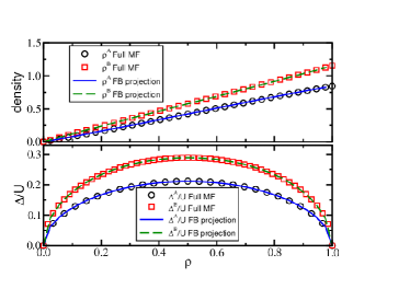
Figure 9: (Color online) Mean field parameters $\Delta^{\alpha}/U$ and densities $\rho^{\alpha}$ vs the total density $\rho$, extrapolated to $U=0$. Lines: our projection on the flat band; symbols: Full multi-band mean field.