Blurs Behave Like Ensembles:
Spatial Smoothings to Improve Accuracy, Uncertainty, and Robustness

Abstract

Neural network ensembles, such as Bayesian neural networks (BNNs), have shown success in the areas of uncertainty estimation and robustness. However, a crucial challenge prohibits their use in practice. BNNs require a large number of predictions to produce reliable results, leading to a significant increase in computational cost. To alleviate this issue, we propose spatial smoothing, a method that spatially ensembles neighboring feature map points of convolutional neural networks. By simply adding a few blur layers to the models, we empirically show that spatial smoothing improves accuracy, uncertainty estimation, and robustness of BNNs across a whole range of ensemble sizes. In particular, BNNs incorporating spatial smoothing achieve high predictive performance merely with a handful of ensembles. Moreover, this method also can be applied to canonical deterministic neural networks to improve the performances. A number of evidences suggest that the improvements can be attributed to the stabilized feature maps and the smoothing of the loss landscape. In addition, we provide a fundamental explanation for prior works—namely, global average pooling, pre-activation, and ReLU6—by addressing them as special cases of spatial smoothing. These not only enhance accuracy, but also improve uncertainty estimation and robustness by making the loss landscape smoother in the same manner as spatial smoothing.

lemmathm lemma propthm prop

1 Introduction

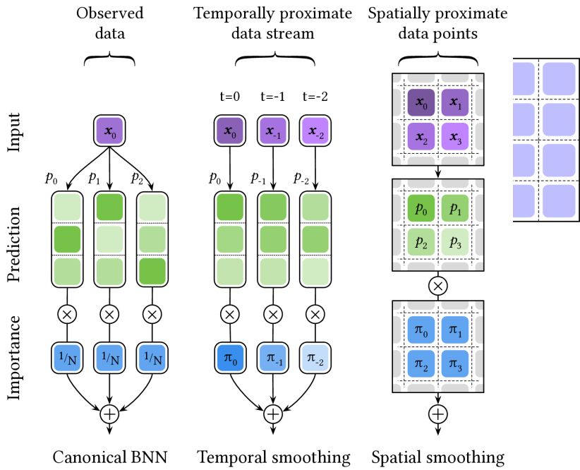
Figure 1: Comparison of three different neural network ensembles: canonical BNN inference, temporal smoothing (Park et al., 2021), and spatial smoothing (ours). In this figure, $\bm{x}_{0}$ is observed data, $p_{i}$ is predictions $p(\bm{y}|\bm{x}_{0},\bm{w}_{i})$ or $p(\bm{y}|\bm{x}_{i},\bm{w}_{i})$, $\pi_{i}$ is importances $\pi(\bm{x}_{i}|\bm{x}_{0})$, and $N$ is ensemble size.

In a real-world environment where many unexpected events occur, machine learning systems cannot be guaranteed to always produce accurate predictions. In order to handle this issue, we make system decisions more reliable by considering estimated uncertainties, in addition to predictions. Uncertainty quantification is particularly crucial in building a trustworthy system in the field of safety-critical applications, including medical analysis and autonomous vehicle control. However, canonical deep neural networks (NNs)—or deterministic NNs—cannot produce reliable estimations of uncertainties (Guo et al., 2017), and their accuracy is often severely compromised by natural data corruptions from noise, blur, and weather changes (Engstrom et al., 2019; Azulay & Weiss, 2019).

Bayesian neural networks (BNNs), such as Monte Carlo (MC) dropout (Gal & Ghahramani, 2016), provide a probabilistic representation of NN weights. They aggregate a number of models selected based on weight probability to make predictions of desired results. Thanks to this feature, BNNs have been widely used in the areas of uncertainty estimation (Kendall & Gal, 2017) and robustness (Ovadia et al., 2019). They are also promising in other fields like out-of-distribution detection (Malinin & Gales, 2018) and meta-learning (Yoon et al., 2018).

Nevertheless, there remains a significant challenge that prohibits their use in practice. BNNs require an ensemble size of up to fifty to achieve high predictive performance, which results in a fiftyfold increase in computational cost (Kendall & Gal, 2017; Loquercio et al., 2020). Therefore, if BNNs can achieve high predictive performance merely with a handful of ensembles, they could be applied to a much wider range of areas.

1.1 Preliminary

We would first like to discuss canonical BNN inference in detail, then move on to vector quantized BNN (VQ-BNN) inference (Park et al., 2021), an efficient approximated BNN inference.

Ensemble averaging for a single data point.

Suppose we have access to model uncertainty, i.e., posterior probability of NN weight $p(\bm{w}|\mathcal{D})$ for training dataset $\mathcal{D}$. The predictive result of BNN is given by the following predictive distribution:

$$p(\bm{y}|\bm{x}_{0},\mathcal{D})=\int p(\bm{y}|\bm{x}_{0},\bm{w})\,p(\bm{w}|\mathcal{D})\,d\bm{w}$$ (1)

where $\bm{x}_{0}$ is observed input data vector, $\bm{y}$ is output vector, and $p(\bm{y}|\bm{x},\bm{w})$ is the probabilistic prediction parameterized by the result of NN for an input $\bm{x}$ and weight $\bm{w}$. In most cases, the integral cannot be solved analytically. Thus, we use the MC estimator to approximate it as follows:

$$p(\bm{y}|\bm{x}_{0},\mathcal{D})\simeq\sum_{i=0}^{N-1}\frac{1}{N}\,p(\bm{y}|\bm{x}_{0},\bm{w}_{i})$$ (2)

where $\bm{w}_{i}\sim p(\bm{w}|\mathcal{D})$ and $N$ is the number of the samples. This equation indicates that BNN inference is ensemble average of NN predictions for “one observed data point” $\bm{x}_{0}$ as shown on the left of Fig. 1. Using $N$ neural networks in the ensemble would requires $N$ times more computational complexity than one NN execution.

Ensemble averaging for proximate data points.

To reduce the computational cost of BNN inference, VQ-BNN (Park et al., 2021) executes NN for “an observed data point” $\bm{x}_{0}$ only once, and complements the result with previously calculated predictions for “other data points” $\bm{x}_{i}$ as follows:

$$p(\bm{y}|\bm{x}_{0},\mathcal{D})\simeq\sum_{i=0}^{N-1}\pi(\bm{x}_{i}|\bm{x}_{0})\,p(\bm{y}|\bm{x}_{i},\bm{w}_{i})$$ (3)

where $\pi(\bm{x}_{i}|\bm{x}_{0})$ is the importance of data $\bm{x}_{i}$ with respect to the observed data $\bm{x}_{0}$, and it is defined as a similarity between $\bm{x}_{i}$ and $\bm{x}_{0}$. If we have access to previous predictions $\{p(\bm{y}|\bm{x}_{1},\bm{w}_{1}),\cdots\}$, the computational performance of VQ-BNN becomes comparable to that of one NN execution to obtain the newly calculated prediction $p(\bm{y}|\bm{x}_{0},\bm{w}_{0})$. To accurately infer the results, the previous predictions should consist of predictions for “data similar to the observed data”, i.e., $\bm{x}_{i}=\bm{x}_{0}+\bm{\varepsilon}_{i}$ for small but non-zero $\bm{\varepsilon}_{i}$. The distribution of the proximate data points is called data uncertainty (Park et al., 2021).

Thanks to the temporal consistency of real-world data streams, aggregating predictions for similar data in data streams is straightforward. Since temporally proximate data sequences tend to be similar, we can memorize recent predictions and calculates their average using exponentially decreasing importance. In other words, VQ-BNN inference for data streams is simply temporal smoothing of recent predictions as shown in the middle of Fig. 1.

VQ-BNN has two limitations, although it may be a promising approach to obtain reliable results in an efficient way. First, it was only applicable to data streams such as video sequences. Applying VQ-BNN to static images is challenging because it is impossible to memorize all similar images in advance. Second, Park et al. (2021) used VQ-BNN only in the testing phase, not in the training phase. We find that ensembling predictions for similar data helps in NN training by smoothing the loss landscape.

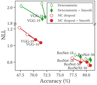
Figure 2: Spatial smoothing improves both accuracy and uncertainty (NLL). Smooth means spatial smoothing. Downward from left to the right ($\searrow$) means better accuracy and uncertainty.

1.2 Main Contribution

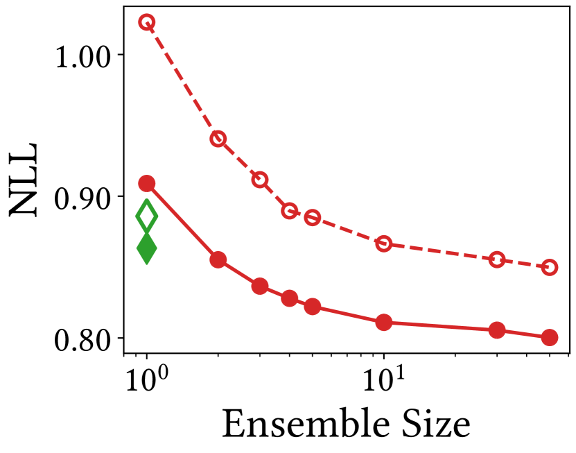
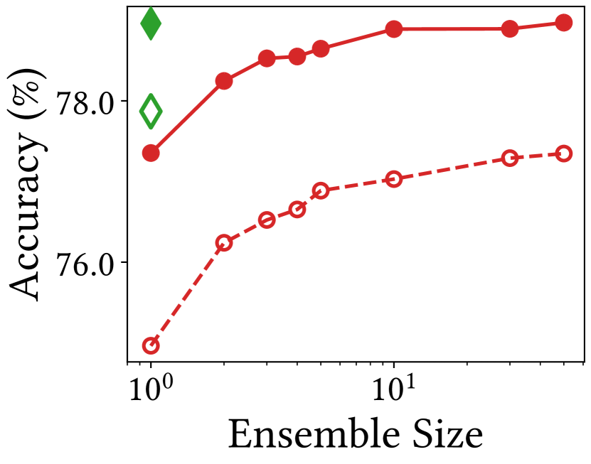
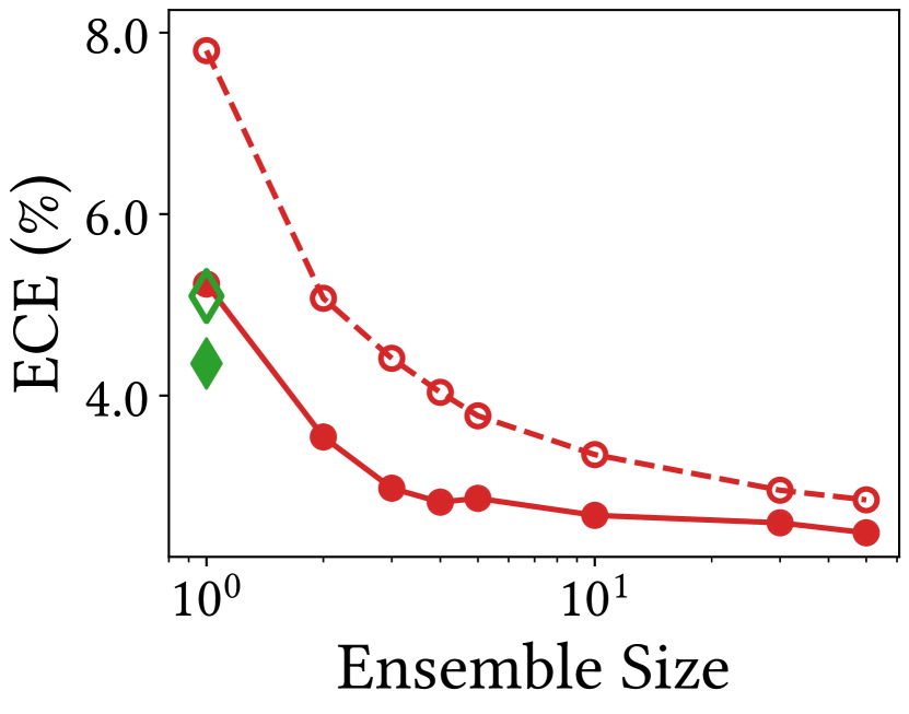
Figure 3: Spatial smoothing improves both accuracy and uncertainty across a whole range of ensemble sizes. We report the predictive performance of ResNet-18 on CIFAR-100. See also Fig. E.1 for results on ImageNet.

Our main contribution is threefold:

Spatially neighboring points in visual imagery tend to be similar, as do feature maps of convolutional neural networks (CNNs). By exploiting this spatial consistency, we propose spatial smoothing as a method of aggregating nearby feature maps to improve the efficiency of ensemble size in BNN inference. The right side of Fig. 1 visualizes spatial smoothing averaging neighboring feature maps.

We empirically demonstrate that spatial smoothing improves the ensemble efficiency in vision tasks, such as image classification on CIFAR and ImageNet datasets, without any additional training parameters. Figure 3 shows that negative log-likelihood (NLL) of “MC dropout + spatial smoothing” with an ensemble size of two is comparable to that of vanilla MC dropout with an ensemble size of fifty. We also demonstrate that spatial smoothing improves accuracy, uncertainty, and robustness all at the same time. Figure 2 shows that spatial smoothing improves both the accuracy and uncertainty of various deterministic and Bayesian NNs with an ensemble size of fifty on CIFAR-100.

Global average pooling (GAP) (Lin et al., 2014; Zhou et al., 2016), pre-activation (He et al., 2016b), and ReLU6 (Krizhevsky & Hinton, 2010; Sandler et al., 2018) have been widely used in vision tasks. However, their motives are largely justified by the experiments. We provide an explanation for these methods by addressing them as special cases of spatial smoothing. Experiments support the claim by showing that the methods improve not only accuracy but also uncertainty and robustness.

2 Probabilistic Spatial Smoothing

To improve the computational performance of BNN inference, VQ-BNN (Park et al., 2021) executes NN prediction only once and complements the result with previously calculated predictions as discussed in Section 1.1. The key to the success of this approach largely depends on the collection of previous predictions for proximate data. Gathering temporally proximate data and their predictions from data streams is easy because recent data and predictions can be aggregated using temporal consistency. On the other hand, gathering time-independent proximate data, e.g. images, is more difficult because they lack such consistency.

2.1 Module Architecture for Ensembling Neighboring Feature Map Points

 

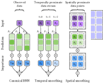
Figure 4: Stages of CNNs such as ResNet (left) and the stages incorporating spatial smoothing layer (right).

So instead of temporal consistency, we use spatial consistency—where neighboring pixels of images are similar—for real-world images. Under this assumption, we take the feature maps as predictions and aggregate neighboring feature maps.

Most CNN architectures, including ResNet, consist of multiple stages that begin with increasing the number of channels while reducing the spatial dimension of the input volume. We decompose an entire BNN inference into several steps by rewriting each stage in a recurrence relation as follows:

$$p(\bm{z}_{i+1}|\bm{z}_{i},\mathcal{D})=\int p(\bm{z}_{i+1}|\bm{z}_{i},\bm{w}_{i})\,p(\bm{w}_{i}|\mathcal{D})\,d\bm{w}_{i}$$ (4)

where $\bm{z}_{i}$ is input volume of the $i$-th stage, and the first and the last volume are input data and output. $\bm{w}_{i}$ and $p(\bm{w}_{i}|\mathcal{D})$ are NN weight in the $i$-th stage and its probability. $p(\bm{z}_{i+1}|\bm{z}_{i},\bm{w}_{i})$ is output probability of $\bm{z}_{i+1}$ with respect to the input volume $\bm{z}_{i}$. To derive the probability from the output feature map, we transform each point of the feature map into a Bernoulli distribution. To do so, a composition of tanh and ReLU, a function from value of range $[-\infty,\infty]$ into probability, is added after each stage. Put shortly, we use neural networks for point-wise binary feature classification.

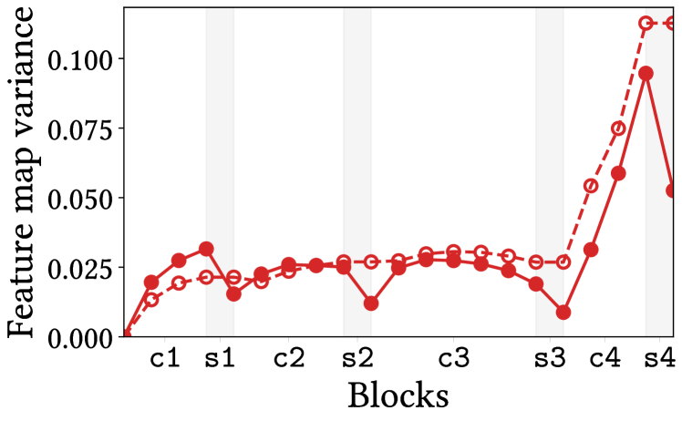
(a) Model uncertainty

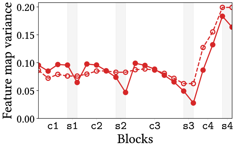
(b) Data uncertainty

Figure 5: Spatial smoothings (gray area) reduce feature map variances, suggesting that they ensemble feature map points. We provide standard deviations of feature maps by block depth with ResNet-50 on CIFAR-100. c1 to c4 and s1 to s4 each stand for stages and spatial smoothing layers. The standard deviations are averaged over the channels. Left: Model uncertainty is represented by the average standard deviation of several feature maps obtained from multiple NN executions. Right: Data uncertainty is represented by the standard deviation of feature map points obtained from one NN execution.

Since Eq. 4 is a kind of BNN inference, it can be approximated using Eq. 3. In other words, each stage predicts feature map points only once and complements predictions with similar but slightly different feature maps. Under spatial consistency, it averages probabilities of spatially neighboring feature map points, which is well known as blur operation in image processing. For the sake of implementation simplicity, average pooling with a kernel size of 2 and a stride of 1 is used as a box blur. This operation aggregates four neighboring probabilities with the same importances.

In summary, as shown in Fig. 4, we propose the following probabilistic spatial smoothing layer:

$$\texttt{Smooth}(\bm{z})=\texttt{Blur}\circ\texttt{Prob}\,(\bm{z})$$ (5)

where $\texttt{Prob}(\cdot)$ is a point-wise function from a feature map to probability, and $\texttt{Blur}(\cdot)$ is importance-weighted average for aggregating spatially neighboring probabilities from feature maps. This Smooth layer is added before each downsampling layers, so we use four Smooth layers for ResNet. Prob and Blur are further elaborated below.

(a) Frequency mask

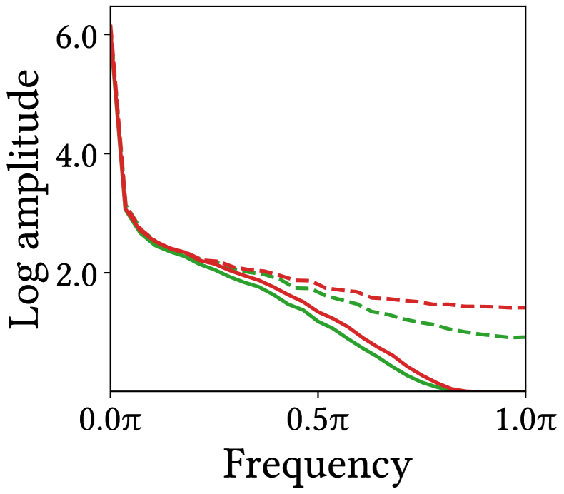
(b) Log amplitude at c1

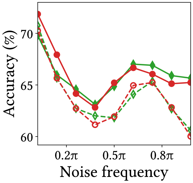
(c) Robustness for noise frequency

Figure 6: MC dropout adds high-frequency noises, and spatial smoothing filters high-frequency signals. In these experiments, we use ResNet-50 for ImageNet. Left: Frequency mask $\textbf{M}_{f}$ with $w=0.1\pi$. Middle: Diagonal components of Fourier transformed feature maps at the end of the stage 1. Right: The accuracy against frequency-based random noise. ResNets are vulnerable to high-frequency noises. Spatial smoothing improves the robustness against high-frequency noises.

Prob: Feature map to probability.

Prob is a function that transforms a real-valued feature map into probability. We use tanh–ReLU composition for this purpose. However, tanh is commonly known to suffer from the vanishing gradient problem. To alleviate this issue, we propose the following temperature-scaled tanh:

$$\texttt{tanh}_{\tau}(\bm{z})=\tau\,\texttt{tanh}\,(\bm{z}/\tau)$$ (6)

where $\tau$ is a hyperparameter called temperature. $\tau$ is $1$ in conventional tanh and $\infty$ in identity function. $\texttt{tanh}_{\tau}$ imposes an upper bound on a value, but does not limit the upper bound to 1.

An unnormalized probability, ranging from $0$ to $\tau$, is allowed as the output of Prob. Then, thanks to the linearity of integration, we obtain an unnormalized predictive distribution accordingly. Taking this into account, we propose the following Prob:

$$\texttt{Prob}(\bm{z})=\texttt{ReLU}\circ\,\texttt{tanh}_{\tau}(\bm{z})$$ (7)

where $\tau>1$. We empirically determine $\tau$ to minimize NLL, a metric that measures both accuracy and uncertainty.

We expect other upper-bounded functions, such as $\texttt{ReLU6}(\bm{z})=\texttt{ReLU}\circ\texttt{min}(\bm{z},6)$ and feature map scaling $\bm{z}/\tau$ with $\tau>1$ which is BatchNorm, to be able to replace $\texttt{tanh}_{\tau}$ in Prob; and as expected, these alternatives improve uncertainty estimation in addition to accuracy. See Section C.2 and Section C.3 for detailed discussions on activation ($\texttt{ReLU}\circ\texttt{BatchNorm}$) and ReLU6 as Prob.

Blur: Averaging neighboring probabilities.

Blur averages the probabilities from feature maps. We primarily use the average pool with a kernel size of 2 and a stride of 1 as the implementation of Blur for the sake of simplicity. Nevertheless, we could generalize Blur by using the following depth-wise convolution, which acts on each input channel separately, with non-trainable kernel

$$\bm{K}=\frac{1}{||\bm{k}||_{1}^{2}}\,\bm{k}\otimes\bm{k}^{\top}$$ (8)

where $\bm{k}$ is a one-dimentional matrix, such as $\bm{k}\in\{\left(1\right),\left(1,1\right),\left(1,2,1\right),\left(1,4,6,4,1\right),\cdots\}$. Different $\bm{k}$s derive different importances for neighboring feature maps. We experimentally show that most Blurs improve the predictive performance. The optimal $\bm{K}$ varies by model, suggesting that the experimental results in this paper have a potential for improvement.

2.2 How Does Spatial Smoothing Help Optimization?

We demonstrate that spatial smoothing has the key properties of ensembles: it reduces feature map variances, filters high-frequency signals, and smoothens loss landscapes. In addition to the improved robustness against MC dropout, which randomly deletes spatial information (cf. Veit et al. (2016)), these empirical perspectives suggest that spatial smoothing behaves like ensembles. Since these properties are the positive attributes that can be expected from ensembles, spatial smoothing can be regarded as ensembles.

Feature map variance.

BNNs have two types of uncertainties: One is model uncertainty and the other is data uncertainty (Park et al., 2021), the distribution of feature map points. Such randomness increases the variance of feature maps. To show that spatial smoothing aggregates the feature maps, we use the following proposition:

Proposition .

Ensembles reduce the variance of predictions.

Proof is omitted since it is straightforward. In our context, predictions are output feature map points of a stage. We investigate model and data uncertainties of the predictions along NN layers to show that spatial smoothing reduces randomnesses and ensembles feature maps. Figure 5 shows the model uncertainty and data uncertainty of Bayesian ResNets including MC dropout layers. In this figure, the uncertainty of MC dropout’s feature map only accumulates, and almost monotonically increases in every NN layer. In contrast, the uncertainty of the feature map of “MC dropout + spatial smoothing” significantly decreases in the spatial smoothing layers, suggesting that the smoothing layers ensemble the feature map. In other words, they make the feature map more accurate and stabilized input volumes for the next stages. Deterministic NNs do not have model uncertainty but data uncertainty. Therefore, spatial smoothing improves the performance of deterministic NNs as well as Bayesian NNs.

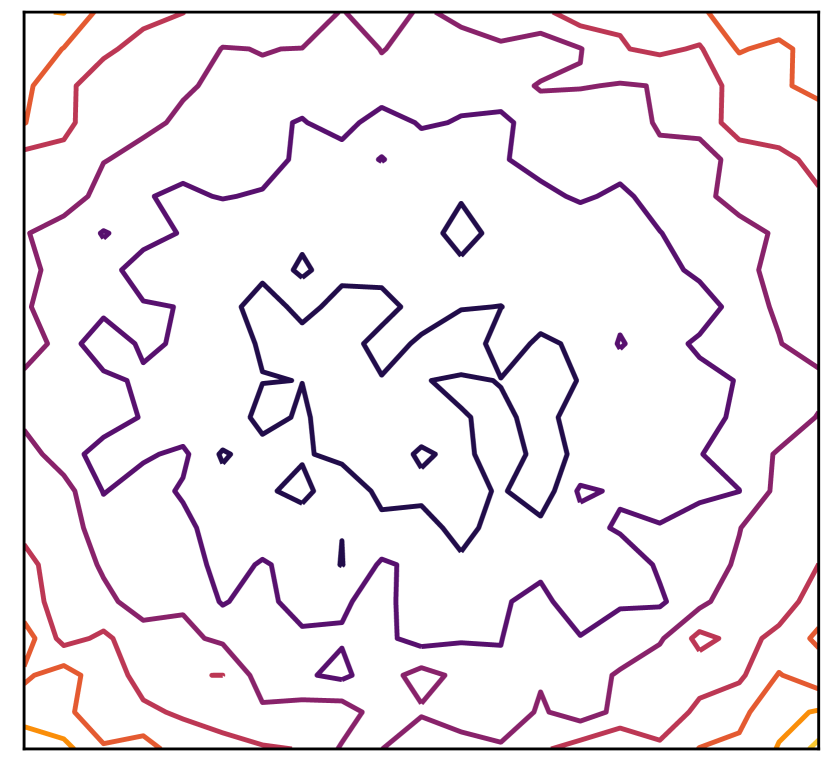
(a) MLP classifier

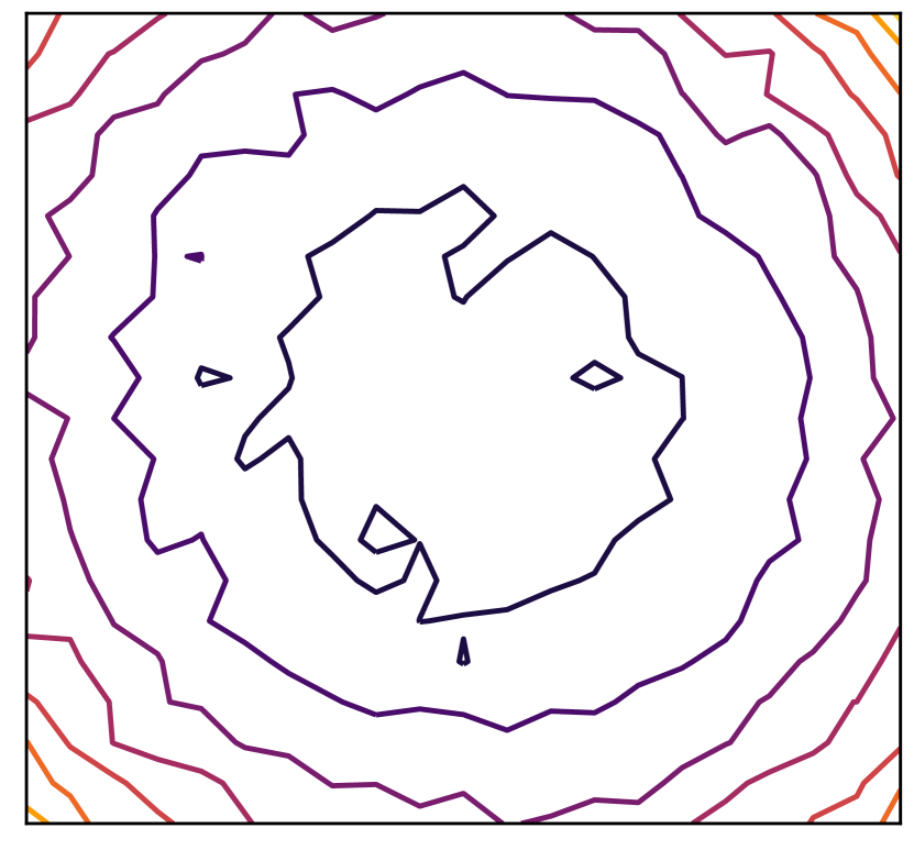
(b) GAP classifier (vanilla)

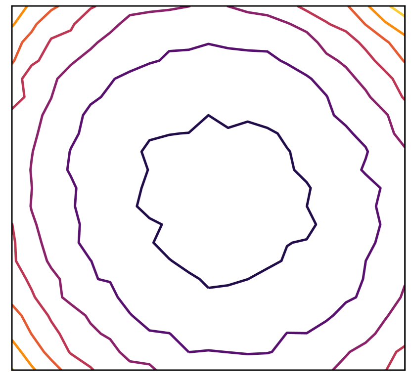
(c) GAP classifier + Smooth

Figure 7: Both GAP and spatial smoothing smoothen the loss landscapes. To demonstrate this, we present the loss landscape visualizations of ResNet-18 models with MC dropout on CIFAR-100.

Fourier analysis.

We also analyze spatial smoothing through the lens of Fourier transform:

Proposition .

Ensembles filter high-frequency signals.

Proof is provided in Section D.2. Figure 6(b) shows the two-dimensional Fourier transformed output feature map at the end of the stage 1. It reveals that MC dropout has almost no effect on the low-frequency ($<0.3\pi$) ranges, but adds high-frequency ($\geq 0.3\pi$) noises. Since spatial smoothing is a low-pass filter, it effectively filters high-frequency signals, including the noises caused by MC dropout.

We also find that CNNs are particularly vulnerable to high-frequency noises. To demonstrate this claim, following Shao et al. (2021), we measure accuracy with respect to data with frequency-based random noise $\bm{x}_{\text{noise}}=\bm{x}_{0}+\mathcal{F}^{-1}\left(\mathcal{F}(\delta)\odot\textbf{M}_{f}\right)$, where $\bm{x}_{0}$ is clean data, $\mathcal{F}(\cdot)$ and $\mathcal{F}^{-1}(\cdot)$ are Fourier transform and inverse Fourier transform, $\delta$ is Gaussian random noise, and $\textbf{M}_{f}$ is frequency mask as shown in Fig. 6(a). Figure 6(c) exhibits the results. In sum, the results show that high-frequency noises significantly impair accuracy. Spatial smoothing improves the robustness by effectively removing high-frequency noises, including those caused by MC dropout.

Loss landscape.

Lastly, we show that randomness hinders NN training, and ensembles help optimization:

Proposition .

The randomness of predictions sharpens the loss landscapes, and ensembles flatten them.

Proof is provided in Section D.3. Since a sharp loss function disturbs NN optimization (Keskar et al., 2017; Santurkar et al., 2018; Foret et al., 2021), reducing the randomness helps NNs learn strong representations. Ensembles with multiple NN predictions in training phases flatten the loss function by averaging out the randomness. Consequently, an ensemble of BNN outputs in training phases significantly improves the predictive performance. See Fig. D.3 for numerical results. However, we do not use this training phase ensemble because it significantly increases training time. We use spatial smoothing instead since it ensembles feature map points without adding training time.

We visualizes the loss landscapes (Li et al., 2018), i.e., the contours of NLL on training datasets. Figure 7(b) shows that the loss landscapes of MC dropout fluctuate and have irregular surfaces due to randomness. As Li et al. (2018); Foret et al. (2021) pointed out, this may lead to poor generalization and predictive performance. Spatial smoothing reduces randomness, as discussed above, and spatial smoothing aids optimization by stabilizing and flattening the loss landscapes of BNNs, as shown in Fig. 7(c).

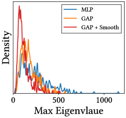
Figure 8: Both GAP and spatial smoothing suppress large Hessian eigenvalue outliers, i.e., they flatten the loss landscapes. Compare with Fig. 7.

Furthermore, we use Hessian to quantitatively represent the sharpness of loss landscapes. The larger the Hessian eigenvalue, the sharper the loss landscape. To efficiently investigate the Hessian eigenvalues of the models in Fig. 7, we propose “Hessian max eigenvalue spectrum”. A detailed description of the Hessian max eigenvalue spectra method is provided in Section A.3. The results of the experiments with a batch size of 128 are provided in Fig. 8, which consistently show that spatial smoothing reduces the magnitude of Hessian eigenvalues and suppresses outliers. Since large Hessian eigenvalues disturb NN training (Ghorbani et al., 2019), we arrive at the same conclusion that spatial smoothing helps NN optimization. In addition, we propose the conjecture that the flatter the loss landscape, the better the uncertainty estimation, and vice versa.

2.3 Revisiting Global Average Pooling

Table 1: MLP does not overfit the training dataset. We report training NLL ($\text{NLL}_{\text{train}}$) and testing NLL ($\text{NLL}_{\text{test}}$) of ResNet-50 on CIFAR-100.

Classifier	$\text{NLL}_{\text{train}}$	$\text{NLL}_{\text{test}}$
GAP	0.0061	0.822
MLP	0.0071	1.029

The success of GAP classifier in image classification is indisputable. The initial motivation and the most widely accepted explanation for this success is that GAP prevents overfitting by using far fewer parameters than multi-layer perceptron (MLP) (Lin et al., 2014). However, we discover that the explanation is poorly supported. We compares GAP with other classifiers including MLP. Contrary to popular belief, Table 1 suggests that MLP does not overfit the training dataset. MLP underfits or gives comparable performance to GAP on the training dataset. On the test dataset, GAP provides better results compared with MLP. See Table C.1 for more detailed results.

Our argument is that GAP is an extreme case of spatial smoothing. In other words, GAP is successful because it aggregates feature map points and smoothens the loss landscape to help optimization. To support this claim, we visualizes the loss landscape of MLP as shown in Fig. 7(a). It is chaotic compared to that of GAP as shown in Fig. 7(b). In conclusion, averaging feature maps tends to help neural networks learn strong representations. Hessian shows the consistent results as demonstrated by Fig. 8.

3 Experiments

This section presents two experiments. The first experiment is image classification through which we show that spatial smoothing not only improves the ensemble efficiency, but also the accuracy, uncertainty, and robustness of both deterministic NN and MC dropout. The second experiment is semantic segmentation on data streams through which we show that spatial smoothing and temporal smoothing (Park et al., 2021) are complementary. In all experiments, we report the average of three evaluations, and the standard deviations are significantly smaller than the improvements. See Appendix A for more detailed configurations.

Three metrics are measured in these experiments: NLL ($\downarrow$), accuracy ($\uparrow$), and expected calibration error (ECE, $\downarrow$) (Guo et al., 2017). NLL represents both accuracy and uncertainty, and is the most widely used as a proper scoring rule. ECE measures discrepancy between accuracy and confidence.

3.1 Image Classification

We mainly discuss ResNet (He et al., 2016a) in image classification, but various models—e.g., VGG (Simonyan & Zisserman, 2015), ResNeXt (Xie et al., 2017), and pre-activation models (He et al., 2016a)—on various datasets—e.g., CIFAR-{10, 100} and ImageNet—show the same trend as shown in Table E.1. Spatial smoothing also improves deep ensemble (Lakshminarayanan et al., 2017), another non-Bayesian probabilistic NN method, as shown in Fig. E.1.

Performance.

Figure 3 shows the predictive performances of ResNet-18 on CIFAR-100. The results indicate that spatial smoothing improves both accuracy and uncertainty in many respects. Let us be more specific. First, spatial smoothing improves the efficiency of ensemble size. In these examples, the NLL of “MC dropout + spatial smoothing” with an ensemble size of 2 is comparable to or even better than that of MC dropout with an ensemble size of 50. In other words, “MC dropout + spatial smoothing” is 25$\times$ faster than MC dropout with a similar predictive performance. Second, the predictive performance of “MC dropout + spatial smoothing” is better than that of MC dropout, at an ensemble size of 50. As discussed in Section 2.2, flat loss landscapes in training phase lead to better performance. Third, spatial smoothing improves the predictive performance of deterministic NN, as well as MC dropout.

Robustness.

Table 2: Spatial smoothing and temporal smoothing are complementary. We provide predictive performance of MC dropout in semantic segmentation. Spat and Temp each stand for spatial smoothing and temporal smoothing. Acc and Cons stand for accuracy and consistency. The numbers in brackets denote the performance improvements over the baseline.

Spat	Temp	NLL	Acc (%)	ECE (%)	Cons (%)
$\cdot$	$\cdot$	0.298 (-0.000)	92.5 (+0.0)	4.20 (-0.00)	95.4 (+0.0)
✓	$\cdot$	0.284 (-0.014)	92.6 (+0.1)	3.96 (-0.24)	95.6 (+0.2)
$\cdot$	✓	0.273 (-0.025)	92.6 (+0.1)	3.23 (-0.97)	96.4 (+1.0)
✓	✓	0.260 (-0.038)	92.6 (+0.1)	2.71 (-1.49)	96.5 (+1.1)

To evaluate robustness against data corruption, we measure predictive performance of ResNet-18 on CIFAR-100-C (Hendrycks & Dietterich, 2019). This dataset consists of data corrupted by 15 different types, each with 5 levels of intensity each. We use mean corruption NLL (mCNLL, $\downarrow$), the averages of NLL over intensities and corruption types, to summarize the performance of corrupted data in a single value. See Eq. 101 for a rigorous definition.

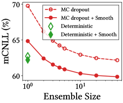
Figure 9: Spatial smoothing improves corruption robustness. We report mCNLL of ResNet-18 on CIFAR-100-C.

Figure 9 shows that spatial smoothing not only improves the efficiency but also corruption robustness across a whole range of ensemble size. See Fig. E.2 for more detailed results. Likewise, spatial smoothing also improves adversarial robustness and perturbation consistency ($\uparrow$) (Hendrycks & Dietterich, 2019; Zhang, 2019), shift-transformation invariance. See Table E.2, Table E.3, and Fig. E.3 for more details.

3.2 Semantic Segmentation

Table 2 summarizes the result of semantic segmentation on CamVid dataset (Brostow et al., 2008) that consists of real-world 360$\times$480 pixels videos. The table shows that spatial smoothing improves predictive performance, which is consistent with the image classification experiment. Moreover, the result reveals that spatial smoothing and temporal smoothing (Park et al., 2021) are complementary. See Table E.4 for more detailed results.

4 Related Work

Spatial smoothing can be compared with prior works in the following areas.

Anti-aliased CNNs.

Local means (Zhang, 2019; Zou et al., 2020; Vasconcelos et al., 2020; Sinha et al., 2020) were introduced for the shift-invariance of deterministic CNNs in image classification. They were motivated to prevent the aliasing effect of subsampling, and used variants of Blur alone. Although these local filtering can result in a loss of information, Zhang (2019) experimentally observed an increase in accuracy that was beyond expectation.

However, we show that the predictive performance improvement of anti-aliased CNNs is not due to anti-aliasing effect of local mean. In particular, Prob plays a key role in the improvement of the predictions as discussed in Appendix F, and the performance improvement of anti-aliased CNNs is due to the cooperation of Blur and activation as Prob, which was not intended in prior works. Several experimental results, e.g., Fig. F.1, support this claim by showing that Blur that does not cooperate with activation harms their predictive performance, and adding Prob before Blur surprisingly improves NNs. Furthermore, our spatial smoothing, which exploits Prob, significantly outperforms Sinha et al. (2020)’s anti-aliased CNN by up to +6.1 percent point on CIFAR-100 in accuracy.

We provide a fundamental explanation for this phenomenon: spatial smoothing (Prob–Blur) behaves like an ensemble. An ensemble not only improves accuracy, but also uncertainty and robustness of deterministic and Bayesian NNs (Lakshminarayanan et al., 2017; Wilson & Izmailov, 2020). For a discussion on non-local means (Wang et al., 2018) and self-attention (Dosovitskiy et al., 2021), see Section 5.

Sampling-free BNNs.

Sampling-free BNNs (Hernández-Lobato & Adams, 2015; Wang et al., 2016; Wu et al., 2019) predict results based on a single or couple of NN executions. To this end, it is assumed that posterior and feature maps follow Gaussian distributions. However, the discrepancy between reality and assumption accumulates in every NN layer. Consequently, to the best of our knowledge, most of the sampling-free BNNs could only be applied to shallow models, such as LeNet, and were tested on small datasets. Postels et al. (2019) applied sampling-free BNNs to SegNet; nonetheless, Park et al. (2021) argued that they do not predict well-calibrated results.

Efficient deep ensembles.

Deep ensemble (Lakshminarayanan et al., 2017; Fort et al., 2019) is another probabilistic NN approach for predicting reliable results. BatchEnsemble (Wen et al., 2020; Dusenberry et al., 2020) ensembles over a low-rank subspace to make deep ensemble more efficient. Depth uncertainty network (Antoran et al., 2020) aggregates feature maps from different depths of a single NN to predict results efficiently. Despite being robust against data corruption, it provides weaker predictive performance compared to deterministic NN and MC dropout.

5 Discussion

We propose spatial smoothing, a non-trainable module motivated by a spatial ensemble, for improving NNs. Three different aspects—namely, feature map variance, Fourier analysis, and loss landscapes—show that spatial smoothing behaves like an ensemble that aggregates neighboring feature maps. The module is simple yet efficient, suggesting that exploiting spatial consistency is important. This novel perspective will shape future work in an interesting way.

The limitation of spatial smoothing is that designing its components requires inductive bias. In other words, the optimal shape of the blur kernel is model-dependent. We believe this problem can be solved by introducing self-attention (Vaswani et al., 2017). Self-attentions for computer vision (Dosovitskiy et al., 2021), also known as Vision Transformers, can be deemed as trainable importance-weighted ensembles of feature maps. Therefore, using self-attentions to generalize spatial smoothing would be a promising work (e.g., Park & Kim (2022)) because it not only expands our work, but also helps deepen our understanding of self-attentions.

Appendix Overview

Appendix A provide comprehensive resources, such as experimental details, to ensure reproducibility. In particular, Appendix A provides the specifications of all models used in this work and detailed hyperparameter setups. Code is available at https://github.com/xxxnell/spatial-smoothing.

Appendix B provides the results of ablation studies. We report the predictive performances of Prob and Blur with various hyperparameters, and investigate several types of edge cases.

Appendix C further discusses prior works—namely, global average pooling, pre-activation, and ReLU6—as special cases of spatial smoothing. In particular, we provide numerical results to demonstrate that these methods improve accuracy, uncertainty estimation, and robustness simultaneously.

Appendix D mainly provides rigorous discussions of three key properties of ensembles: Section 2.2, Section 2.2, and Section 2.2. If a NN has these three properties at the same time, we can infer that the NN exploits the ensemble effect. Since these properties are necessary conditions for ensembles, they can be regarded as a checklist for ensembles.

Appendix E provides detailed results of experiments, e.g., image classification and semantic segmentation. The results include predictive performances on various settings and robustness on corrupted datasets.

Appendix F demonstrates that Prob plays an important role in spatial smoothing. Blur alone can improve predictive performance of conventional CNNs only when activation ($\texttt{ReLU}\circ\texttt{BatchNorm}$) acts as Prob; however, otherwise, Blur harms the predictive performance. For example, Blur degrades the performance of pre-activation CNNs.

Appendix A Experimental Setup and Datasets

We obtain the main experimental results with the Intel Xeon W-2123 Processor, 32GB memory, and a single GeForce RTX 2080 Ti for CIFAR (Krizhevsky et al., 2009) and CamVid (Brostow et al., 2008). For ImageNet (Russakovsky et al., 2015), we use AMD Ryzen Threadripper 3960X 24-Core Processor, 256GB memory, and four GeForce RTX 2080 Ti. We conduct ablation studies with four Intel Intel Broadwell CPUs, 15GB memory, and a single NVIDIA T4. Models are implemented in PyTorch (Paszke et al., 2019). The detailed configurations of image classification and semantic segmentation are as follows.

A.1 Image Classification

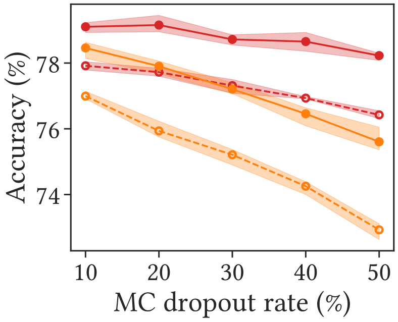
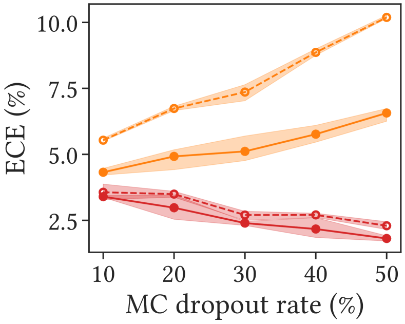
Figure A.1: Spatial smoothing improves predictive performance at all dropout rates. As the dropout rate increases, both accuracy and ECE decrease. The performance is optimized when accuracy and uncertainty are balanced.

We use VGG (Simonyan & Zisserman, 2015), ResNet (He et al., 2016a), pre-activation ResNet (He et al., 2016a), and ResNeXt (Xie et al., 2017) in image classification. According to the structure suggested by Zagoruyko & Komodakis (2016), each block of Bayesian NNs contains one MC dropout layer.

NNs are trained using categorical cross-entropy loss and SGD optimizer with initial learning rate of 0.1, momentum of 0.9, and weight decay of $5\times 10^{-4}$. We also use multi-step learning rate scheduler with milestones at 60, 130, and 160, and gamma of 0.2 on CIFAR, and with milestones at 30, 60, and 80, and gamma of 0.2 on ImageNet. We train NNs for 200 epochs with batch size of 128 on CIFAR, and for 90 epochs with batch size of 256 on ImageNet. We start training with gradual warmup (Goyal et al., 2017) for 1 epoch on CIFAR. Basic data augmentations, namely random cropping and horizontal flipping, are used. One exception is the training of ResNeXt on ImageNet. In this case, we use the batch size of 128 and learning rate of 0.05 because of memory limitation.

We use hyperparameters that minimizes NLL of ResNet: $\tau=10$, and MC dropout rate of 30% for CIFAR and 5% for ImageNet. We use $|\bm{k}|=2$ for the sake of implementation simplicity. For fair comparison, models with and without spatial smoothing share hyperparameters such as MC dropout rate. However, Fig. A.1 shows that spatial smoothing improves predictive performance of ResNet-18 at all dropout rates on CIFAR-100. The default ensemble size of MC dropout is 50. We report averages of three evaluations, and error bars in figures represent min and max values. Standard deviations are omitted from tables for better visualization. See source code for other details.

A.2 Semantic Segmentation

We use U-Net (Ronneberger et al., 2015) in semantic segmentation. Following Bayesian SegNet (Kendall et al., 2017), Bayesian U-Net contains six MC dropout layers. We add spatial smoothing before each subsampling layer in U-Net encoder. We use 5 previous predictions and decay rate of $e^{-0.8}\simeq 45\%$ per frame for temporal smoothing.

CamVid consists of 720$\times$960 pixels road scene video sequences. We resize the image bilinearly to 360$\times$480 pixels. We use a list reduced to 11 labels by following previous works, e.g. (Kendall & Gal, 2017).

NNs are trained using categorical cross-entropy loss and Adam optimizer with initial learning rate of $0.001$ and $\beta_{1}$ of 0.9, and $\beta_{2}$ of 0.999. We train NN for 130 epoch with batch size of 3. The learning rate decreases to $0.0002$ at the 100 epoch. Random cropping and horizontal flipping are used for data augmentation. Median frequency balancing is used to mitigate dataset imbalance. Other details follow Park et al. (2021).

A.3 Hessian Max Eigenvalue Spectrum

We investigate Hessians to evaluate the smoothness of the loss landscapes quantitatively. In particular, we calculate Hessian eigenvalue spectrum (Ghorbani et al., 2019)—distributions of Hessian eigenvalues—to show how spatial smoothing helps NN optimization. The most widely known method to obtain the Hessian eigenvalues is the stochastic Lanczos quadrature algorithm. This algorithm finds representative Hessian eigenvalues for full batch. However, it requires a lot of memory and computing resources, so it is not feasible for many practical NNs.

In order to quantitatively evaluate loss landscapes, an efficient Hessian eigenvalue investigation method is needed. In the training phase, we calculate the mean gradients with respect to mini-batches, rather than the entire dataset. Therefore, it may be reasonable to investigate the properties of the Hessian “mini-batch-wisely”. Among those Hessians, large Hessian eigenvalues dominates NN training (Ghorbani et al., 2019). Based on these insights, we propose an efficient method, Hessian max eigenvalue spectrum, that evaluates the distribution of “the maximum Hessian eigenvalues for mini-batchs”. To obtain Hessian max eigenvalue spectrum, we use power iteration (PowerIter) to produce only the largest (or top-$k$) eigenvalue of the Hessian. Then, we visualize the spectrum by aggregating the largest eigenvalues for mini-batches. For example, we gather top-1 Hessian eigenvalues for Fig. 8. We summarize the algorithm in Algorithm 1.

Note that Hessian must be calculated for “regularized losses” on “augmented datasets”, since NN training optimizes NLL + $\ell_{2}$ regularization on augmented datasets—not NLL on clean datasets; measuring Hessian eigenvalues on clean dataset would give incorrect results.

Algorithm 1   Hessian max eigenvalue spectrum

0:  training dataset $\mathcal{D}$, mini-batch size $|\mathcal{B}|$, number of eigenvalues per mini-batch $k$, loss with regularizations (e.g., $\ell_{2}$ regularization) $\mathcal{L}(\cdot)$, NN weight $\bm{w}$, data augmentation $g(\cdot)$

0:  Hessian max eigenvalue spectrum $\mathcal{H}=\{\lambda^{(1)}_{1},\lambda^{(1)}_{2},\cdots,\lambda^{(2)}_{1},\lambda^{(2)}_{2},\cdots\}$ where $\lambda^{(i)}_{j}$ is the $j^{\text{th}}$ largest Hessian eigenvalues for the $i^{\text{th}}$ mini-batch

1:  $\mathcal{H}=\{\}$

2:  for $i^{\text{th}}$ mini-batch $\mathcal{B}^{(i)}$ in $\mathcal{D}$ do

3:     ${\{\lambda^{(i)}_{1},\cdots,\lambda^{(i)}_{k}\}\leftarrow}$ $\hskip 30.00005pt{\texttt{PowerIter}\left(k,\text{Hessian of }\mathcal{L}(\bm{w},g(\mathcal{B}^{(i)}))\right)}$

4:     $\mathcal{H}\leftarrow\mathcal{H}\,\bigcup\,\{\lambda^{(i)}_{1},\cdots,\lambda^{(i)}_{k}\}$

5:  end for

This algorithm is easy to implement and requires significantly less memory and computational cost, compared with stochastic Lanczos quadrature algorithm with respect to entire dataset. With this method, we can investigate the Hessian of large NNs, which would require a lot of GPU memory. In this paper, we use both Hessian eigenvalue spectra using stochastic Lanczos quadrature algorithm and Hessian max eigenvalue spectrum using power iteration implemented by Yao et al. (2020). Compare Fig. C.3 and Fig. 8.

Appendix B Ablation Study

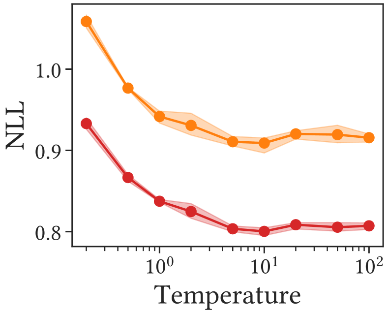
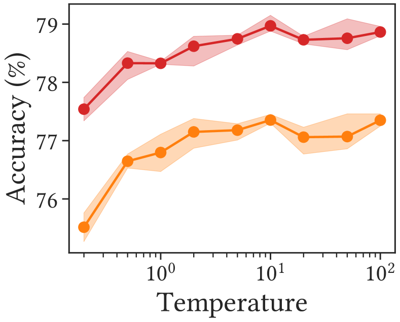
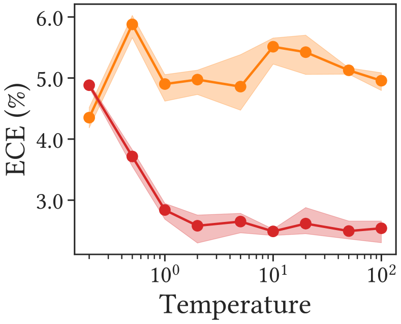
Figure B.1: The temperature controls the trade-off between accuracy and uncertainty. The accuracy increases as the temperature increases, but predictions become more overconfident.

Probabilistic spatial smoothing proposed in this paper consists of two components: Prob and Blur. This section explores several candidates for each component and their properties.

B.1 Prob: Feature Maps to Probabilities

Table B.1: We use tanh as the default for Prob based on the predictive performance of MC dropout for CIFAR-100 with various Probs.

Model	Smooth	NLL	Acc (%)	ECE (%)
VGG-16	$\cdot$	1.133 (-0.000)	68.8 (+0.0)	3.66 (+0.00)
	ReLU $\circ$ tanh	1.064 (-0.069)	70.4 (+1.6)	2.99 (-0.67)
	ReLU $\circ$ ReLU6	1.093 (-0.040)	69.8 (+1.0)	4.26 (+0.60)
	ReLU $\circ$ Constant	0.995 (-0.138)	72.5 (+3.7)	2.11 (-1.55)
	Blur	0.985 (-0.000)	72.4 (+0.0)	1.77 (+0.00)
	Blur $\circ$ ReLU $\circ$ tanh	0.984 (-0.001)	72.7 (+0.3)	2.07 (+0.30)
	Blur $\circ$ ReLU $\circ$ ReLU6	0.982 (-0.003)	72.5 (+0.1)	1.84 (+0.07)
	Blur $\circ$ ReLU $\circ$ Constant	0.991 (+0.005)	72.9 (+0.5)	1.03 (-0.74)
VGG-19	$\cdot$	1.215 (-0.000)	67.3 (+0.0)	6.37 (+0.00)
	ReLU $\circ$ tanh	1.131 (-0.084)	69.2 (+1.9)	5.23 (-1.14)
	ReLU $\circ$ ReLU6	1.166 (-0.049)	68.3 (+1.0)	6.44 (-0.06)
	ReLU $\circ$ Constant	0.997 (-0.218)	72.5 (+5.2)	1.09 (-5.29)
	Blur	1.039 (-0.000)	71.1 (+0.0)	3.12 (+0.00)
	Blur $\circ$ ReLU $\circ$ tanh	1.034 (-0.005)	71.3 (+0.2)	3.31 (+0.19)
	Blur $\circ$ ReLU $\circ$ ReLU6	1.038 (-0.002)	71.3 (+0.2)	3.84 (+0.72)
	Blur $\circ$ ReLU $\circ$ Constant	0.995 (-0.045)	72.3 (+1.2)	1.41 (-1.71)
ResNet-18	$\cdot$	0.848 (-0.000)	77.3 (+0.0)	3.01 (+0.00)
	ReLU $\circ$ tanh	0.838 (-0.010)	77.7 (+0.4)	2.92 (-0.08)
	ReLU $\circ$ ReLU6	0.844 (-0.004)	77.4 (+0.1)	2.74 (-0.27)
	ReLU $\circ$ Constant	0.825 (-0.023)	77.7 (+0.4)	1.87 (-1.14)
	Blur	0.806 (-0.000)	78.6 (+0.0)	2.56 (+0.00)
	Blur $\circ$ ReLU $\circ$ tanh	0.801 (-0.005)	78.9 (+0.3)	2.56 (-0.01)
	Blur $\circ$ ReLU $\circ$ ReLU6	0.805 (-0.001)	78.9 (+0.2)	2.59 (+0.03)
	Blur $\circ$ ReLU $\circ$ Constant	0.811 (+0.005)	78.5 (-0.2)	1.84 (-0.72)
ResNet-50	$\cdot$	0.822 (-0.000)	79.1 (+0.0)	6.63 (+0.00)
	ReLU $\circ$ tanh	0.812 (-0.010)	79.3 (+0.2)	6.74 (+0.11)
	ReLU $\circ$ ReLU6	0.799 (-0.023)	79.4 (+0.3)	6.71 (+0.08)
	ReLU $\circ$ Constant	0.788 (-0.034)	79.6 (+0.5)	5.22 (-1.41)
	Blur	0.798 (-0.000)	80.0 (+0.0)	7.21 (+0.00)
	Blur $\circ$ ReLU $\circ$ tanh	0.800 (+0.002)	80.1 (+0.1)	7.25 (+0.04)
	Blur $\circ$ ReLU $\circ$ ReLU6	0.800 (+0.002)	80.2 (+0.2)	7.30 (+0.09)
	Blur $\circ$ ReLU $\circ$ Constant	0.779 (-0.019)	80.4 (+0.4)	5.81 (-1.40)

We define Prob as a composition of an upper-bounded function and ReLU, a function that imposes the lower bound of zero. There are several widely used upper-bounded functions: $\texttt{tanh}_{\tau}(\bm{x})=\tau\,\texttt{tanh}(\bm{x}/\tau)$, $\texttt{ReLU6}(\bm{x})=\texttt{max}(\texttt{min}(\bm{x},6),0)$, and constant scaling which is $\bm{x}/\tau$.

Table B.1 shows the predictive performance improvement by Prob with various upper-bounded functions on CIFAR-100. In this experiment, we use models with MC dropout, and $\tau=5$ for constant scaling. The results indicate that upper-bounded functions with ReLU tend to improve accuracy and uncertainty at the same time. In addition, they show that Prob and Blur are complementary; the best results are obtained when using both Prob and Blur. For the main experiments, we use the composition of $\texttt{tanh}_{\tau}$ and ReLU as Prob although constant scaling outperforms in some cases. This is because the hyperparameter of constant scaling is highly dependent on dataset and model.

Temperature.

The characteristics of temperature-scaled tanh depends on $\tau$. This $\texttt{tanh}_{\tau}$ has a couple of useful properties: $\texttt{tanh}_{\tau}$ has an upper bound of $\tau$, and the first derivative of $\texttt{tanh}_{\tau}$ at $x=0$ does not depend on $\tau$.

Figure B.1 shows the predictive performance of ResNet-18 with MC dropout and spatial smoothing for the temperature on CIFAR-100. In this figure, the accuracy increases as the temperature increases. In contrast, in terms of ECE, NN predicts more underconfident results as $\tau$ decreases. NLL, a metric representing both accuracy and uncertainty, is minimized when the accuracy and the uncertainty are balanced. In conclusion, we set the default value of $\tau$ to 10.

It is a misinterpretation that the result is overconfident at low $\tau$ because ECE is high. By definition, ECE relies on the absolute value of the difference between confidence and accuracy. In this example, at low $\tau$, the accuracy is greater than the confidence, which leads to a high ECE. Moreover, at $\tau=0.2$, ECE with $N=50$ is greater than that with $N=1$, which means that the result is severely underconfident.

B.2 Blur: Averaging Neighboring Probabilities

Table B.2: The optimal shape of the blur kernel is model-dependent. We measure the predictive performance of MC dropout using spatial smoothing with various size of Blur kernels on CIFAR-100.

Model	$|\bm{k}|$	NLL	Acc (%)	ECE (%)
VGG-16	1	1.087 (-0.000)	69.8 (+0.0)	3.43 (-0.00)
	2	1.034 (-0.053)	71.4 (+1.6)	1.06 (-2.37)
	3	0.986 (-0.101)	72.7 (+2.9)	1.03 (-2.40)
	5	1.018 (-0.069)	72.0 (+2.2)	1.32 (-2.11)
VGG-19	1	1.096 (-0.000)	69.8 (+0.0)	4.74 (-0.00)
	2	1.071 (-0.025)	70.4 (+0.6)	2.15 (-2.59)
	3	1.026 (-0.070)	71.9 (+2.1)	2.56 (-2.18)
	5	1.032 (-0.064)	71.6 (+1.8)	2.16 (-2.58)
ResNet-18	1	0.840 (-0.000)	77.6 (+0.0)	2.63 (-0.00)
	2	0.801 (-0.039)	78.9 (+1.4)	2.56 (-0.07)
	3	0.822 (-0.018)	78.7 (+1.1)	2.86 (-0.23)
	5	0.837 (-0.003)	78.4 (+0.8)	3.05 (-0.42)
ResNet-50	1	0.814 (-0.000)	79.5 (+0.0)	6.56 (-0.00)
	2	0.806 (-0.008)	80.0 (+0.5)	7.35 (+0.79)
	3	0.796 (-0.019)	79.9 (+0.4)	7.38 (+0.82)
	5	0.816 (+0.001)	79.4 (-0.1)	7.38 (+0.82)

Blur is a depth-wise convolution with a normalized kernel. The kernel given by Eq. 8 is derived from various $\bm{k}$s such as $\bm{k}\in\{\left(1\right),\left(1,1\right),\left(1,2,1\right),\left(1,4,6,4,1\right),\cdots\}$. In these examples, if $|\bm{k}|$ is 1, Blur is identity. If $|\bm{k}|$ is 2, Blur is a box blur, which is used in the main experiments. If $|\bm{k}|$ is 3 or 5, Blur is an approximated Gaussian blur.

Table B.2 shows predictive performance of models using spatial smoothing with the kernels on CIFAR-100. This results show that most kernels improve both accuracy and uncertainty. The most effective kernel size depends on the model.

B.3 Position of Spatial Smoothing

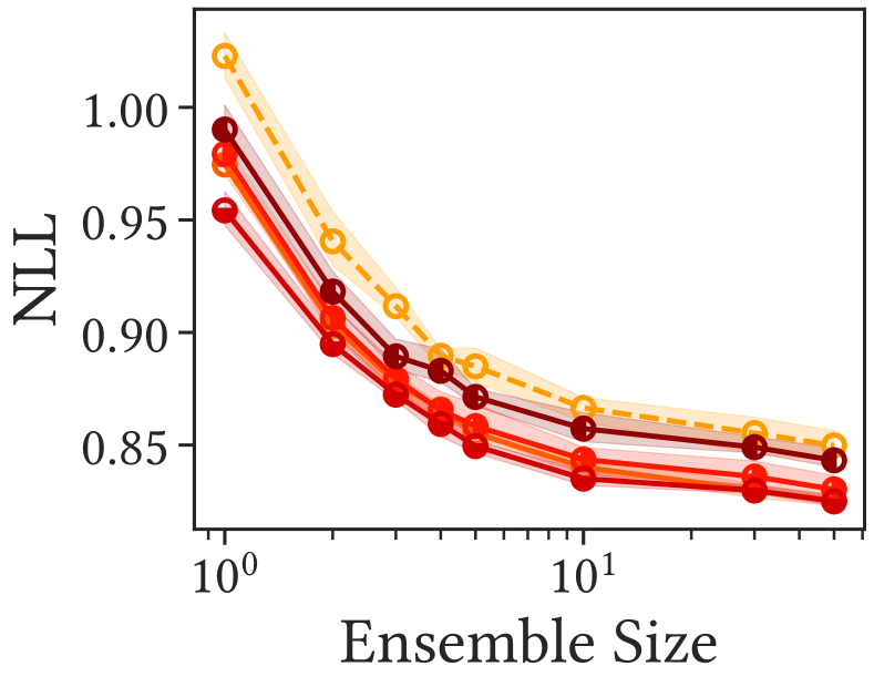
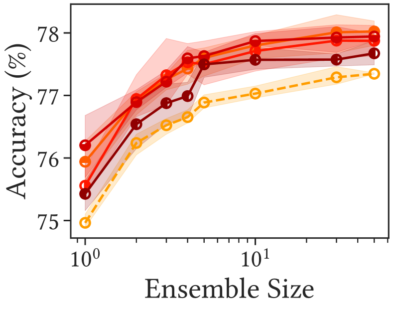
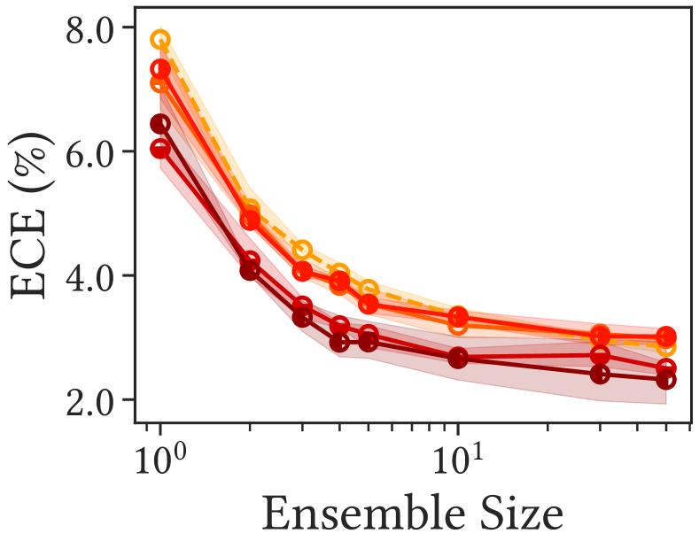
Figure B.2: Spatial smoothing close to the last layer (s3) significantly improves performance. We report predictive performance of ResNet-18 with one spatial smoothing after each stage on CIFAR-100. None indicates vanilla MC dropout.

As shown in Fig. 5, the magnitude of feature map uncertainty tends to increase as the depth increases. Therefore, we expect that spatial smoothing close to the output layer will mainly drive performance improvement.

We investigate the predictive performance of models with MC dropout using only one spatial smoothing layer. Figure B.2 shows the predictive performance of ResNet-18 with one spatial smoothing after each stage on CIFAR-100. The results suggest that spatial smoothing after s3 is the most important for improving performance. Surprisingly, spatial smoothing after s4 is the least important. This is because GAP, the most extreme case of spatial smoothing, already exists there.

Appendix C Revisiting Prior Works

As mentioned in Section 2, prior works—namely, GAP, pre-activation, and ReLU6—are spacial cases of spatial smoothing. This section discusses them in detail.

C.1 Global Average Pooling

The composition of GAP and a fully connected layer is the most popular classifier in classification tasks. The original motivation and the most widely accepted explanation for the success is that GAP classifier prevents overfitting because it uses significantly fewer parameters than MLP (Lin et al., 2014). To disprove this claim, we measure the predictive performance of MLP, GAP, and global max pooling (GMaxP), a classifier that uses the same number of parameters as GAP, on training dataset.

Predictive performance.

Table C.1: MLP classifier does not overfit training dataset, i.e., GAP does not regularize NNs. We provide predictive performance of MC dropout with various classifiers on CIFAR-100. Err is error.

Model	Classifier	Train				Test
		NLL	Err (%)	ECE (%)		NLL	Acc (%)	ECE (%)
VGG-16	GAP	0.0852	0.461	6.75		1.030	72.3	3.24
	MLP	0.5492	13.1	13.8		1.133	68.8	3.66
	GMaxP	0.0846	0.470	6.67		1.050	72.2	3.60
	GMedP	0.0867	0.501	6.80		1.042	72.2	3.35
VGG-19	GAP	0.1825	2.50	10.4		1.035	71.9	1.46
	MLP	0.7144	17.7	14.8		1.215	67.3	6.37
	GMaxP	0.1939	2.85	10.6		1.063	71.5	2.10
	GMedP	0.1938	2.80	10.6		1.051	71.7	1.70
ResNet-18	GAP	0.0124	0.0287	1.19		0.841	77.5	2.92
	MLP	0.0076	0.0347	7.22		1.040	74.8	9.55
	GMaxP	0.0113	0.0233	1.41		0.905	76.3	5.23
	GMedP	0.0156	0.0347	1.46		0.889	76.4	5.03
ResNet-50	GAP	0.0061	0.0220	0.48		0.822	79.1	6.63
	MLP	0.0071	0.0370	8.53		1.029	76.9	11.8
	GMaxP	0.0074	0.0313	1.09		0.887	77.2	5.67
	GMedP	0.0053	0.0287	0.47		0.849	78.5	6.29

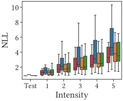
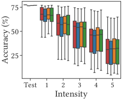
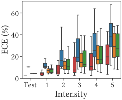
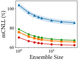
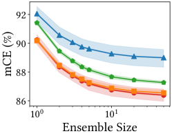
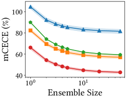
Figure C.1: GAP classifier improves not only the predictive performance on clean dataset but also the robustness. We measure the predictive performance of ResNet-18 using MC dropout with classifiers on CIFAR-100-C.

Table C.1 shows the experimental results on the training and the test dataset of CIFAR-100, suggesting that the explanation is poorly supported. On both the training and the test dataset, most predictive performance of MLP is worse than that of GAP. It is a counter-intuitive result meaning that MLP do not overfit the training dataset. In addition, the performance improvement by GAP is remarkable in VGG, which has irregular loss landscape. The predictive performance of GMaxP is better than that of MLP, but worse than that of GAP. This shows that using fewer parameters partially helps to improve predictive performance; however, it is insufficient to explain the predictive performance improvement by GAP. Finally, global median pooling (GMedP) provides better predictive performance than GMaxP. It implies that using other noise reduction methods also helps, in part, to improve predictive performance.

Robustness.

To evaluate the robustness of the classifiers, we measure the predictive performance of ResNet-18 using MC dropout with the classifiers on CIFAR-100-C. Figure C.1 shows the experimental results suggesting that MLP is not robust against data corruption, as we would expect. In terms of accuracy, the robustness of GMaxP and GMedP is relatively comparable to that of GAP; however, in terms of uncertainty, GAP is the most robust. These are consistent results with other spatial smoothing experiments.

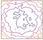
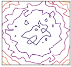
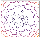
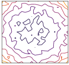
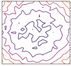
(a) MLP classifier

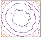
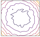
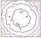
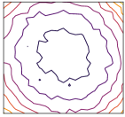
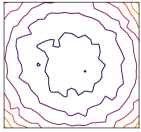
(b) GAP classifier

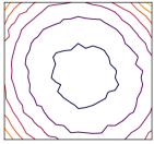
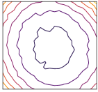
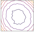
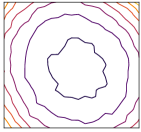
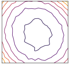
(c) GAP classifier + Smooth

Figure C.2: GAP and spatial smoothing smoothen the loss landscapes. We visualize the loss landscape sequences of ResNet-18 with MC dropout on CIFAR-100. Although each sequence shares the bases, it fluctuates due to the randomness.

Loss landscape visualization.

To understand the mechanism of GAP performance improvement, we investigate the loss landscape. Figure C.2 shows the loss landscape sequences of ResNet with MC dropout. In this figure, each sequence shares the bases, but they fluctuate due to the randomness of the MC dropout. Figure 2(a) is the loss landscape of the model using MLP classifier instead of GAP classifier. This loss landscape is chaotic and irregular, resulting in hindering and destabilizing NN optimization. Fig. 2(b) is loss landscape sequence of ResNet with GAP classifier. Since GAP ensembles all of the feature map points at the last stage, it flattens and stabilizes the loss landscape. Likewise, as shown in Fig. 2(c), spatial smoothing layers at the end of all stages also flattens and stabilizes the loss landscape.

Hessian eigenvalue spectra.

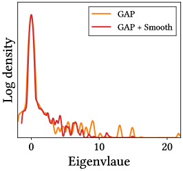
Figure C.3: Spatial smoothing suppress eigenvalue outliers. We provide Hessian eigenvalue spectra of ResNet-18 with MC dropout on CIFAR-100. Compare with Fig. 8.

Figure 8 shows the Hessian max eigenvalue spectra of MLP classifier model and GAP classifier models with and without spatial smoothing layers. As Li et al. (2018); Foret et al. (2021) and Section D.3 pointed out, Hessian eigenvalue outliers disturb NN training. This figure explicitly show that the GAP and spatial smoothing reduce the magnitude of the Hessian eigenvalues and suppress the outliers, which leads to the same conclusion as the previous visualizations: GAP as well as spatial smoothing smoothen the loss landscapes. In conclusion, averaging feature map points tends to help neural network optimization by smoothing, flattening, and stabilizing the loss landscape. We observe a similar phenomenon for deterministic NNs. We also provide the Hessian eigenvalue spectrum as shown in Fig. C.3, and it leads to the same conclusion.

In these experiments, we use MLP incorporating dropout layers with a rate of 50% as the classifier. Since the dropout is one of the factors that makes MLP underfit the training dataset, we also evaluate MLP without dropouts. Nevertheless, the results still shows that the predictive performance of MLP is worse than that of GAP on the training dataset. Moreover, it severely degrades predictive performance of ResNet on the test dataset.

C.2 Pre-activation

He et al. (2016b) experimentally showed that the pre-activation arrangement, in which the activation $\texttt{ReLU}\circ\texttt{BatchNorm}$ is placed before the convolution, improves the accuracy of ResNet. Since $\gamma$s of most BatchNorms in CNNs are near-zero (Frankle et al., 2021), BatchNorms reduce the magnitude of feature maps. Constant scaling is a non-trainable BatchNorm with no bias, and it also reduces the magnitude of feature map. In Table B.1, we show that constant scaling improves predictive performance. Considering the similarity between Prob with constant scaling and conventional activation, i.e., the similarity between $\texttt{ReLU}\circ\texttt{ConstantScaling}$ and $\texttt{ReLU}\circ\texttt{BatchNorm}$, we find that the pre-activation arrangement improves uncertainty as well as accuracy, because convolutions act as a Blur.

To demonstrate this, we change the post-activation of all layers to pre-activation, and measure the predictive performance. Table C.2 shows the predictive performance of various models with pre-activation. The results suggests that pre-activation improves both accuracy and uncertainty in most cases. For VGG-19, pre-activation significantly degrades accuracy but improves NLL. In conclusion, they imply that pre-activation is a special case of spatial smoothing.

Santurkar et al. (2018) argued that BatchNorm helps in optimization by flattening the loss landscape. Likewise, we show that spatial smoothing flattens and smoothens the loss landscapes. It will be interesting to rigorously investigate if BatchNorm helps in ensembling feature maps.

C.3 ReLU6

ReLU6 was empirically introduced to improve predictive performance (Krizhevsky & Hinton, 2010). Sandler et al. (2018) used “ReLU6 as the nonlinearity because of its robustness when used with low-precision computation”. In Table B.1, we show that ReLU6s at the end of stages helps to ensemble spatial information by transforming the feature map to Bernoulli distributions. Since spatial smoothing improves robustness against data corruption, it seems reasonable that ReLU6 is robust to low-precision computation. A more abundant investigation is promising future works.

We measure the predictive performance of NNs using all activations as ReLU6 instead of ReLU. However, in contrast to the results in Table B.1, the results are not consistent. We speculate that the reason is that a lot of ReLU6s overly regularize NNs.

Table C.2: Pre-activation arrangement improves uncertainty as well as accuracy. We measure the predictive performance of models with pre-activation arrangement on CIFAR-100.

Model	MC dropout	Pre-act	NLL	Acc (%)	ECE (%)
VGG-16	$\cdot$	$\cdot$	2.047 (-0.000)	71.6 (+0.0)	19.2 (-0.0)
	$\cdot$	✓	1.827 (-0.219)	72.5 (+0.9)	19.8 (+0.6)
	✓	$\cdot$	1.133 (-0.000)	68.8 (+0.0)	3.66 (-0.00)
	✓	✓	1.036 (-0.096)	71.7 (+2.9)	3.55 (-0.11)
VGG-19	$\cdot$	$\cdot$	2.016 (-0.000)	67.6 (+0.0)	21.2 (-0.0)
	$\cdot$	✓	1.799 (-0.217)	64.4 (-3.2)	17.2 (-4.0)
	✓	$\cdot$	1.215 (-0.000)	67.3 (+0.0)	6.37 (-0.00)
	✓	✓	1.084 (-0.131)	70.1 (+3.7)	4.23 (-2.14)
ResNet-18	$\cdot$	$\cdot$	0.983 (-0.000)	77.1 (+0.0)	7.75 (-0.00)
	$\cdot$	✓	0.934 (-0.049)	77.6 (+0.5)	8.04 (+0.29)
	✓	$\cdot$	0.937 (-0.000)	76.9 (+0.0)	5.11 (-0.00)
	✓	✓	0.872 (-0.065)	77.6 (+0.7)	5.53 (+0.42)
ResNet-50	$\cdot$	$\cdot$	0.880 (-0.000)	79.0 (+0.0)	8.35 (-0.00)
	$\cdot$	✓	0.870 (-0.010)	79.4 (+0.4)	8.27 (-0.08)
	✓	$\cdot$	0.831 (-0.000)	78.6 (+0.0)	6.06 (-0.00)
	✓	✓	0.819 (-0.012)	79.5 (+0.9)	6.29 (+0.23)

Appendix D Extended Analysis of How Spatial Smoothing Works

This section provides further explanation of the analysis in Section 2.2.

D.1 Neighboring Feature Maps in CNNs Are Similar

Although our work is based on the assumption that images are spatially consistent, we provide one explanation of the spatial consistency of feature maps: even if input images are spatially inconsistent, feature maps are consistent.

Consider a single-layer CNN with one channel:

$$y_{i} =\left[\bm{w}*\bm{x}\right]_{i}=\sum_{l=1}^{k}w_{l}x_{i-l+1}$$ (9)

where $*$ is convolution with a kernel of size $k$, $\bm{y}$ is feature map output, $\bm{w}$ is kernel weight, and $\bm{x}$ is input random variable. Then, the covariance of two neighboring points is:

$$\text{Cov}(y_{i},y_{i+1}) =\text{Cov}(\sum_{l=1}^{k}w_{l}x_{i-l+1},\,\sum_{m=1}^{k}w_{m}x_{i-m+2})$$ (10)

$$=\sum_{l=1}^{k}\sum_{m=1}^{k}w_{l}w_{m}\,\text{Cov}(x_{i-l+1},x_{i-m+2})$$ (11)

$$=\sum_{l=1}^{k-1}w_{l}w_{l+1}\,\sigma^{2}(x_{i-l+2})+\cdots$$ (12)

where $\sigma^{2}(x_{i-l+1})$ is the variance of $x_{i-l+1}$. Therefore, $\text{Cov}(\bm{y}_{i},\bm{y}_{i+1})$ is non-zero for randomly initialized weights. If $\bm{x}$ is iid, i.e., $\text{Cov}(x_{i},x_{j})=\delta_{ij}\sigma^{2}(x_{i})$ where $\delta_{ij}$ is the Kronecker delta, the remainders in Eq. 12 vanish.

(a) single-layer CNN

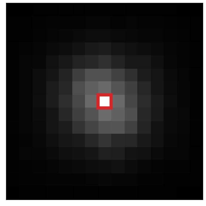
(b) five-layer CNN with ReLU

Figure D.1: Neighboring feature map points in CNNs are similar, even if input values are iid. We provide covariances of feature map points with respect to the center feature map (in the red square). Input values are Gaussian random noise. Left: A single convolutional layer correlates the target feature map with another feature map that is 3 pixels away, since the kernel size is 3$\times$3. Right: A deep CNN more strongly correlates neighboring feature maps.

For example, the covariance of two neighboring feature map points in a CNN with a kernel size of 3 is non-zero, i.e.,

$$\text{Cov}(y_{1},y_{2})=w_{1}w_{2}\,\sigma^{2}(x_{2})+w_{2}w_{3}\,\sigma^{2}(x_{3})$$ (13)

since the terms for $i\neq j$ vanish and only the terms for $i=j$ remain. Therefore, the neighboring feature maps $y_{1}$ and $y_{2}$ are correlated.

Experiment.

To demonstrate the spatial consistency of feature maps empirically, we provide feature map covariances of randomly initialized single-layer CNN and five-layer CNN with ReLU nonlinearity. In this experiment, the input values are Gaussian random noises. As shown in Fig. 1(a), one convolutional layer correlates neighboring feature map points. Fig. 1(b) shows that multiple convolutional layers correlate one feature map with distant feature maps. Moreover, the feature maps in deep CNNs have a stronger relationship with neighboring feature maps.

D.2 Ensembles Filter High-Frequency Signals

Consider a square importance-weight matrix for an ensemble that does not change size. The sum of the matrix columns is one, and all the elements are greater than zero. Therefore, the matrix can be expressed using Softmax, and a Softmax-normalized matrix is a low-pass filter (Wang et al., 2022).

Experiment.

Since blur filter (Blur) is low-pass filter, probabilistic spatial smoothing (Prob–Blur) is also low-pass filter. In Fig. 6(b), at the end of the stage 1, we show that MC dropout adds high-frequency noise to feature maps, and spatial smoothing effectively removes it. We observe the same phenomena at other stages.

In addition, Fig. 6(c) shows that CNNs are vulnerable to high-frequency random noise. Interestingly, it also shows that CNNs are robust against noise with frequencies from $0.6\pi$ to $0.8\pi$, corresponding to approximately 3 pixel periods. Since the receptive fields of convolutions are 3$\times$3, the noise with a period smaller than the size is averaged out by convolutions. For the same reason, convolutions are particularly vulnerable against the noise with a frequency of $0.3\pi$, corresponding to a period of 6 pixel.

D.3 Randomness Sharpens the Loss Landscapes, and Ensembles Smoothen Them

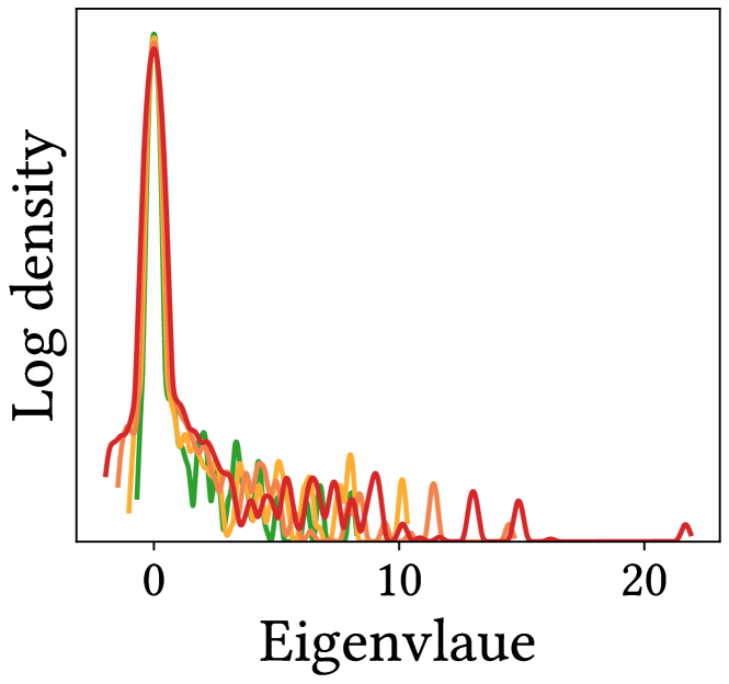
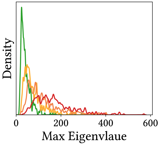
Figure D.2: Randomness due to MC dropout sharpens the loss function. We provide Hessian eigenvalue spectra (left) and Hessian max eigenvalue spectra (right) of ResNet-18 on CIFAR-100.

Ws show that the randomness of NN predictions hinder and destabilize NN training because it causes the loss landscape and its gradient to fluctuate from moment to moment. In other words, the randomness, such as dropout, sharpens the loss landscape. Since ensemble effectively reduces the randomness of predictions, it smoothens the loss landscape. Below, we prove these claims.

Definition of sharpness.

We start with Foret et al. (2021)’s definition of sharpness:

$$\text{sharpness}_{\rho}=\max_{||\bm{\epsilon}||\leq\rho}\mathcal{L}(\bm{w}+\bm{\epsilon})-\mathcal{L}(\bm{w})$$ (14)

where $\mathcal{L}$ is NLL loss on a training dataset, $\bm{w}$ is NN weight, $\bm{\epsilon}$ is small weight perturbation, and $\rho$ is neighborhood radius. However, they used this expression for deterministic optimization tasks, and this expression is not for random variables $\bm{\epsilon}$; the maximum value of a random variable loss $\max_{||\bm{\epsilon}||\leq\rho}\mathcal{L}(\bm{w}+\bm{\epsilon})$ does not appropriately represent the properties of the random variable in many cases. For example, the maximum value of a Gaussian random variable is infinity, but we cannot observe that infinity in practice.

To address this issue, we replace “the maximum value of the loss random variable” with “the expected value of sufficiently large losses” as follows:

$$\max_{||\bm{\epsilon}||\leq\rho}\mathcal{L}(\bm{w}+\bm{\epsilon})\rightarrow\mathbb{E}\left[\max(\mathcal{L}(\bm{w}+\bm{\epsilon}),\mathcal{L}(\bm{w}))\ \Big{|}\ ||\bm{\epsilon}||\leq\rho\right]$$ (15)

where $\mathbb{E}[\ \cdot\ \big{|}\ ||\bm{\epsilon}||\leq\rho]$ is expected value under the constraint $||\bm{\epsilon}||\leq\rho$. Then, the expected sharpness is: so $\mathbb{E}[\text{sharpness}_{\rho}]\geq 0$ by definition. Therefore, as the magnitude of $\bm{\epsilon}$—and dropout rate for MC dropout—increases, the sharpness increases.

This expression can be regarded as the difference between “the large neighborhood losses” and “the average loss” when $\mathcal{L}(\bm{w}+\bm{\epsilon})$ is a Gaussian random variable, i.e., $\mathbb{E}[\mathcal{L}(\bm{w}+\bm{\epsilon})]\simeq\mathbb{E}[\mathcal{L}(\bm{w})]+\mathbb{E}[\bm{\epsilon}^{T}\nabla\mathcal{L}(\bm{w})]\simeq\mathbb{E}[\mathcal{L}(\bm{w})]=\mathcal{L}(\bm{w})$. In other words, this expression connects the sharpness and instability of the loss landscapes in probabilistic NN settings:

$$\begin{aligned} \mathbb{E}[\text{sharpness}_{\rho}]\simeq{}&\underbrace{\mathbb{E}\left[\max(\mathcal{L}(\bm{w}+\bm{\epsilon}),\mathcal{L}(\bm{w}))\ \Big{|}\ ||\bm{\epsilon}||\leq\rho\right]}_{\text{Expected lower-bounded loss in neighborhood}}\\ {}&-\underbrace{\mathbb{E}\left[\mathcal{L}(\bm{w}+\bm{\epsilon})\ \Big{|}\ ||\bm{\epsilon}||\leq\rho\right]}_{\text{Expected loss}}\end{aligned}$$ (16)

Expected sharpness is proportional to the variance of loss.

Let $\rho$ be sufficiently large ($\rho\gg 1$), i.e., we use weak constraints for weight randomness $\bm{\epsilon}$ at fixed $\bm{w}$. If $\mathcal{L}$ is a Gaussian random variable, the expected value of $\max(\mathcal{L}(\bm{w}+\bm{\epsilon}),\mathcal{L}(\bm{w}))$ is the expected value of Rectified Gaussian distribution:

$$\mathbb{E}[\max(\mathcal{L}(\bm{w}+\bm{\epsilon}),\mathcal{L}(\bm{w}))]=\mathbb{E}[\mathcal{L}(\bm{w})]+c\mathbb{V}[\mathcal{L}(\bm{w}+\bm{\epsilon})]^{\nicefrac{{1}}{{2}}}$$ (17)

where $c$ is a positive constant. Therefore, the expected value of sharpness is proportional to the standard deviation of the loss:

$$\mathbb{E}[\text{sharpness}] =\mathbb{E}[\max(\mathcal{L}(\bm{w}+\bm{\epsilon}),\mathcal{L}(\bm{w}))-\mathcal{L}(\bm{w})]$$ (18)

$$=\mathbb{E}[\mathcal{L}(\bm{w})]+c\mathbb{V}[\mathcal{L}(\bm{w}+\bm{\epsilon})]^{\nicefrac{{1}}{{2}}}-\mathbb{E}[\mathcal{L}(\bm{w})]$$ (19)

$$=c\mathbb{V}[\mathcal{L}(\bm{w}+\bm{\epsilon})]^{\nicefrac{{1}}{{2}}}$$ (20)

In conclusion, the expected sharpness is proportional to the variance of loss random variable.

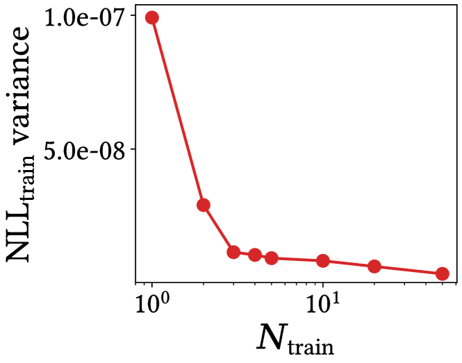
(a) $\mathbb{V}\left[\mathcal{L}\right]$ for ensemble size on training dataset

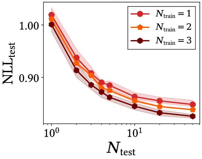
(b) NLL for ensemble size on test dataset

Figure D.3: Training phase ensemble helps NN learn strong representation. Left: The variance of NLL ($\mathbb{V}\left[\mathcal{L}\right]$) on training dataset is inversely proportional to the ensemble size for large $N_{\text{train}}$. See Eq. 26. Right: Training phase ensemble improves the predictive performance on test dataset.

Variance of losses is inversely proportional to the ensemble size.

Let $p_{i}\in\left(0,1\right]$ be a confidence of one NN prediction, and $\bar{p}^{(N)}$ be a confidence of $N$ ensemble, i.e., $\bar{p}^{(N)}=\frac{1}{N}\sum_{i=1}^{N}p_{i}$. Then, the variance of the NLL loss is:

$$\mathbb{V}\left[\mathcal{L}\right] =\mathbb{V}\left[\frac{1}{|\mathcal{D}|}\sum_{\mathcal{D}}-\log\bar{p}^{(N)}\right]$$ (21)

$$=\frac{1}{|\mathcal{D}|}\mathbb{V}\left[-\log\bar{p}^{(N)}\right]$$ (22)

$$\simeq\frac{1}{|\mathcal{D}|}\mathbb{V}\left[-\log\mu+\left(1-\frac{\bar{p}^{(N)}}{\mu}\right)\right]$$ (23)

$$=\frac{1}{|\mathcal{D}|}\mathbb{V}\left[-\frac{\bar{p}^{(N)}}{\mu}\right]$$ (24)

$$=\frac{1}{N}\frac{\mathbb{V}\left[p_{i}\right]}{\mu^{2}|\mathcal{D}|}$$ (25)

$$=\frac{1}{N}\frac{\sigma^{2}_{\text{pred}}}{\mu^{2}|\mathcal{D}|}$$ (26)

where $\mu=\bar{p}^{(\infty)}$ and $\sigma^{2}_{\text{pred}}$ is predictive variance of confidence. We use the formula $\mathbb{V}\left[\frac{1}{N}\sum_{i=1}^{N}\xi\right]=\frac{1}{N}\mathbb{V}\left[\xi\right]$ for arbitrary random variable $\xi$, and we take the first-order Taylor expansion with an assumption $\bar{p}^{(N)}\simeq\mu$ in Eq. 23. Therefore, the approximated sharpness is:

$$\text{sharpness}_{\rho}^{2}\simeq\frac{1}{N}\frac{\sigma^{2}_{\text{pred}}}{\mu^{2}|\mathcal{D}|}$$ (27)

In conclusion, the variance of NLL, (the square of) the sharpness, is proportional to the variance of predictions $\sigma^{2}_{\text{pred}}$ and inversely proportional to the ensemble size $N$. As the ensemble size increases in the training phase, the loss landscape becomes smoother. Flat loss landscape results in better predictive performance and generalization (Foret et al., 2021).

In these explanations, we only consider model uncertainty for the sake of simplicity. Extending the formulations to data uncertainty is straightforward. The predictive distribution of data-complemented BNN inference (Park et al., 2021) is:

$$p(\bm{y}|\mathcal{S},\mathcal{D}) =\int p(\bm{y}|\bm{x},\bm{w})p(\bm{x}|\mathcal{S})p(\bm{w}|\mathcal{D})d\bm{x}d\bm{w}$$ (28)

$$=\int p(\bm{y}|\bm{z})p(\bm{z}|\mathcal{S},\mathcal{D})d\bm{z}$$ (29)

where $\mathcal{S}$ is proximate data distribution, $\bm{z}=(\bm{x},\bm{w})$, and $p(\bm{z}|\mathcal{S},\mathcal{D})=p(\bm{x}|\mathcal{S})\,p(\bm{w}|\mathcal{D})$. This equation clearly shows that $\bm{w}$ and $\bm{x}$ are symmetric. Therefore, we obtain the formulas including both model and data uncertainty by replacing $\bm{w}$ with joint random variable of $\bm{x}$ and $\bm{w}$, i.e. $\bm{w}\rightarrow\bm{z}=(\bm{w},\bm{x})$.

Experiment.

Above, we claim two statements. First, the higher the dropout rate, the sharper the loss landscape. Second, the variance of the loss is inversely proportional to the ensemble size.

To demonstrate the former claim quantitatively, we compare the Hessian eigenvalue spectra and the Hessian max eigenvalue spectra of MC dropout with various dropout rates. In these experiments, we use ensemble size of one for MC dropout. For detailed explanation of Hessian max eigenvalue spectrum, see Section C.1.

Fig. D.2 represents the spectra, which reveals that as the randomness of the model increases, the number of Hessian eigenvalue outliers increases. Since outliers are detrimental to the optimization process (Ghorbani et al., 2019), dropout disturb NN optimization.

To show the latter claim, we evaluate the variance of NLL loss for ensemble size $N_{\text{train}}$ as shown in Fig. 3(a). As we would expect, the variance of the NLL loss—the sharpness of the loss landscape—is inversely proportional to the ensemble size for large $N_{\text{train}}$.

D.4 Training Phase Ensembles Lead to Better Performance

Section D.3 raises an immediate question: Is there a performance difference between “training with prediction ensemble” and “training with a low MC dropout rate, instead of no ensemble”? Note that both methods reduce the sharpness of the loss landscape. This section answers the question by providing theoretical and experimental explanations that the ensemble in the training phase can improve predictive performance.

According to Gal & Ghahramani (2016), the total predictive variance (in regression tasks) is:

$$\sigma^{2}_{\text{pred}}=\sigma^{2}_{\text{model}}+\sigma^{2}_{\text{sample}}$$ (30)

where $\sigma^{2}_{\text{model}}$ is model precision and $\sigma^{2}_{\text{sample}}$ is sample variance. Therefore, the model precision is the lower bound of the predictive variance, i.e.:

$$\sigma^{2}_{\text{pred}}\geq\sigma^{2}_{\text{model}}$$ (31)

The model precision depends only on the model architecture. For example, in the case of MC dropout, $\sigma^{2}_{\text{model}}$ is proportional to the dropout rate (Gal & Ghahramani, 2016) as follows:

$$\sigma^{2}_{\text{model}}\propto\text{dropout rate}$$ (32)

These suggest that model precision dominate predictive variance if the MC dropout rate is large enough, i.e., even if the number of ensembles is increased in the training phase, the predictive variance is almost the same. In contrast, decreasing the MC dropout rate reduces prediction diversity, and it obviously leads to performance degradation. Therefore, in the training phase, it is better to ensemble predictions than to lower the MC dropout rate. We believe that the training phase ensemble is strongly correlated with Batch Augmentation (Hoffer et al., 2020). We leave concrete analysis for future work.

Experiment.

The experiments below support the theoretical analysis. We train MC dropout by using training-phase ensemble method with various ensemble sizes $N_{\text{train}}$. As we would expect, Fig. 3(b) shows that training phase ensemble significantly improves the predictive performance.

We also measure the predictive variances of NLL. The predictive variances of the model with $N_{\text{train}}=1$ and with $N_{\text{train}}=3$ are $\mathbb{V}\left[\mathcal{L}\right]=0.0169$ and $\mathbb{V}\left[\mathcal{L}\right]=0.0179$, respectively. Since the predictive variances of the two models are almost the same, we infer that there exists a lower bound.

Appendix E Extended Informations of Experiments

This section provides additional information on the experiments in Section 3.

E.1 Image Classification

Table E.1: Spatial smoothing improves both accuracy and uncertainty at the same time. Predictive performance of various models with spatial smoothing in image classification on CIFAR-10, CIFAR-100, and ImageNet.

Model & Dataset	MC dropout	Smooth	NLL	Acc (%)	ECE (%)
VGG-19 & CIFAR-10	$\cdot$	$\cdot$	0.401 (-0.000)	93.1 (+0.0)	3.80 (-0.00)
	$\cdot$	✓	0.376 (-0.002)	93.2 (+0.1)	5.49 (+1.69)
	✓	$\cdot$	0.238 (-0.000)	92.6 (+0.0)	3.55 (-0.00)
	✓	✓	0.197 (-0.041)	93.3 (+0.7)	0.68 (-2.86)
ResNet-18 & CIFAR-10	$\cdot$	$\cdot$	0.182 (-0.000)	95.2 (+0.0)	2.75 (-0.00)
	$\cdot$	✓	0.173 (-0.009)	95.4 (+0.2)	2.31 (-0.44)
	✓	$\cdot$	0.157 (-0.000)	95.2 (+0.0)	1.14 (-0.00)
	✓	✓	0.144 (-0.014)	95.5 (+0.2)	1.04 (-0.10)
VGG-16 & CIFAR-100	$\cdot$	$\cdot$	2.047 (-0.000)	71.6 (+0.0)	19.2 (-0.0)
	$\cdot$	✓	1.878 (-0.169)	72.2 (+0.6)	20.5 (+1.3)
	✓	$\cdot$	1.133 (-0.000)	68.8 (+0.0)	3.66 (-0.00)
	✓	✓	1.034 (-0.099)	71.4 (+2.6)	1.06 (-2.60)
VGG-19 & CIFAR-100	$\cdot$	$\cdot$	2.016 (-0.000)	67.6 (+0.0)	21.2 (-0.0)
	$\cdot$	✓	1.851 (-0.165)	71.7 (+4.0)	20.2 (-1.0)
	✓	$\cdot$	1.215 (-0.000)	67.3 (+0.0)	6.37 (-0.00)
	✓	✓	1.071 (-0.144)	70.4 (+3.0)	2.15 (-4.22)
ResNet-18 & CIFAR-100	$\cdot$	$\cdot$	0.886 (-0.000)	77.9 (+0.0)	4.97 (-0.00)
	$\cdot$	✓	0.863 (-0.023)	78.9 (+1.0)	4.40 (-0.57)
	✓	$\cdot$	0.848 (-0.000)	77.3 (+0.0)	3.01 (-0.00)
	✓	✓	0.801 (-0.047)	78.9 (+1.6)	2.56 (-0.45)
ResNet-50 & CIFAR-100	$\cdot$	$\cdot$	0.835 (-0.000)	79.9 (+0.0)	8.88 (-0.00)
	$\cdot$	✓	0.834 (-0.002)	80.7 (+0.8)	9.29 (+0.42)
	✓	$\cdot$	0.822 (-0.000)	79.1 (+0.0)	6.63 (-0.00)
	✓	✓	0.800 (-0.022)	80.1 (+1.0)	7.25 (+0.62)
ResNeXt-50 & CIFAR-100	$\cdot$	$\cdot$	0.804 (-0.000)	80.6 (+0.0)	8.23 (-0.00)
	$\cdot$	✓	0.825 (+0.022)	80.8 (+0.3)	9.41 (+1.18)
	✓	$\cdot$	0.762 (-0.000)	80.5 (+0.0)	5.67 (-0.00)
	✓	✓	0.759 (-0.002)	80.7 (+0.2)	6.62 (+0.94)
ResNet-18 & ImageNet	$\cdot$	$\cdot$	1.210 (-0.000)	70.3 (+0.0)	1.62 (-0.00)
	$\cdot$	✓	1.183 (-0.027)	70.6 (+0.3)	1.22 (-0.40)
	✓	$\cdot$	1.215 (-0.000)	70.0 (+0.0)	1.39 (-0.00)
	✓	✓	1.190 (-0.032)	70.6 (+0.6)	2.25 (+0.86)
ResNet-50 & ImageNet	$\cdot$	$\cdot$	0.949 (-0.000)	76.0 (+0.0)	2.97 (-0.00)
	$\cdot$	✓	0.916 (-0.033)	76.9 (+0.9)	3.46 (+0.49)
	✓	$\cdot$	0.945 (-0.000)	76.0 (+0.0)	1.89 (-0.00)
	✓	✓	0.905 (-0.040)	77.0 (+1.0)	2.49 (+0.60)
ResNeXt-50 & ImageNet	$\cdot$	$\cdot$	0.919 (-0.000)	77.7 (+0.0)	3.63 (-0.00)
	$\cdot$	✓	0.907 (-0.012)	78.0 (+0.3)	4.60 (+0.97)
	✓	$\cdot$	0.895 (-0.000)	77.7 (+0.0)	2.53 (-0.00)
	✓	✓	0.887 (-0.008)	78.1 (+0.4)	3.28 (+0.75)

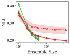
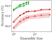
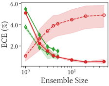
(a) VGG-19 on CIFAR-10

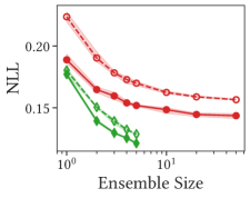
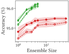
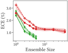
(b) ResNet-18 on CIFAR-10

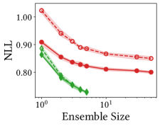
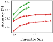
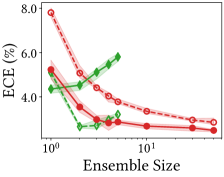
(c) ResNet-18 on CIFAR-100

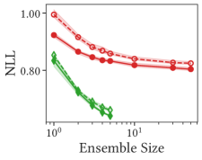
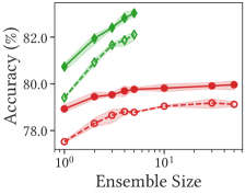
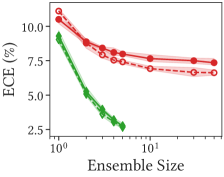
(d) ResNet-50 on CIFAR-100

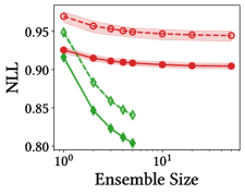
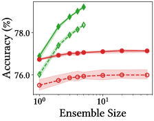
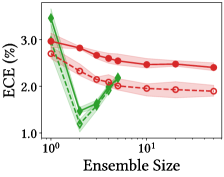
(e) ResNet-50 on ImageNet

Figure E.1: Spatial smoothing improves both accuracy and uncertainty across a whole range of ensemble sizes.

We present numerical comparisons in the image classification experiment and discuss the results in detail.

Computational performance.

The throughput of MC dropout and “MC dropout + spatial smoothing” is 755 and 675 image/sec, respectively, in training phase on ImageNet. As mentioned in Section 3.1, NLL of “MC dropout + spatial smoothing” with ensemble size of 2 is comparable to or even better than that of MC dropout with ensemble size of 50. Therefore, “MC dropout + spatial smoothing” is 22$\times$ faster than MC dropout with similar predictive performance, in terms of throughput.

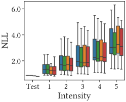
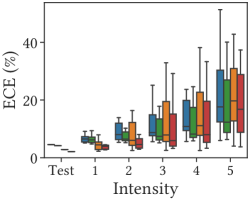
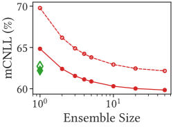
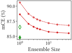
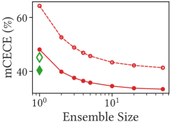
Figure E.2: Spatial smoothing improves corruption robustness. We measure the predictive performance of ResNet-18 on CIFAR-100-C. In the top row, we use an ensemble size of fifty for MC dropout with and without spatial smoothing.

Predictive performance on test dataset.

Table E.1 shows the predictive performance of various deterministic and Bayesian NNs with and without spatial smoothing on CIFAR-10, CIFAR-100, and ImageNet. This table suggests the following: First, spatial smoothing improves both accuracy and uncertainty in most cases. In particular, it improves the predictive performance of all models with MC dropouts. Second, spatial smoothing significantly improves the predictive performance of VGG, compared with ResNet. VGG has a chaotic loss landscape, which results in poor predictive performance (Li et al., 2018), and spatial smoothing smoothens its loss landscape effectively. Third, as the depth increases, the performance improvement decreases. Deeper NNs provide more overconfident results (Guo et al., 2017), but the number of spatial smoothing layers calibrating uncertainty is fixed. Last, the performance improvement of ResNeXt, which includes an ensemble in its internal structure, is relatively marginal.

Fig. E.1 shows predictive performance of MC dropout and deep ensemble for ensemble size. A deep ensemble with an ensemble size of 1 is a deterministic NN. This figure shows that spatial smoothing improves efficiency of ensemble size and the predictive performance at ensemble size of 50. In addition, spatial smoothing reduces the variance in performance, suggesting that it stabilizes NN training.

One peculiarity of the results on ImageNet is that spatial smoothing degrades ECE of ResNet-50. It is because spatial smoothing significantly improves the accuracy in this case, and there tends to be a trade-off between accuracy and ECE, e.g. as shown in (Guo et al., 2017), Fig. A.1, and Fig. B.1. Instead, spatial smoothing shows the improvement in NLL, another uncertainty metric.

Predictive performance on training datasets.

Note that spatial smoothing helps NN learn strong representations. In other words, spatial smoothing does not regularize NNs, and it reduces the training loss. For example, the NLL of ResNet-18 with MC dropout on CIFAR-100 training dataset is $2.20\times 10^{-2}$. The training NLL of the ResNet with spatial smoothing is $1.94\times 10^{-2}$.

Corruption robustness.

We measure predictive performance on CIFAR-100-C (Hendrycks & Dietterich, 2019) in order to evaluate the robustness of the models against 5 intensities and 15 types of data corruption. The top row of Fig. E.2 shows the results as a box plot. This box plot shows the median, interquartile range (IQR), minimum, and maximum of predictive performance for types. They reveal that spatial smoothing improves predictive performance for corrupted data. In particular, spatial smoothing undoubtedly helps in predicting reliable uncertainty.

To summarize the performance of corrupted data in a single value, Hendrycks & Dietterich (2019) introduced a corruption error (CE) for quantitative comparison. $\text{CE}_{c}^{f}$, which is CE for corruption type $c$ and model $f$, is as follows:

$$\text{CE}_{c}^{f}=\left(\sum_{i=1}^{5}E^{f}_{i,c}\right)\bigg{/}\left(\sum_{i=1}^{5}E^{\text{AlexNet}}_{i,c}\right)$$ (100)

where $E^{f}_{i,c}$ is top-1 error of $f$ for corruption type $c$ and intensity $i$, and $E^{\text{AlexNet}}_{i,c}$ is the error of AlexNet. Mean CE or mCE summarizes $\text{CE}_{c}^{f}$ by averaging them over 15 corruption types such as Gaussian noise, brightness, and show. Likewise, to evaluate robustness in terms of uncertainty, we introduce corruption NLL (CNLL, $\downarrow$) and corruption ECE (CECE, $\downarrow$) as follows:

$$\text{CNLL}_{c}^{f}=\left(\sum_{i=1}^{5}\text{NLL}^{f}_{i,c}\right)\bigg{/}\left(\sum_{i=1}^{5}\text{NLL}^{\text{AlexNet}}_{i,c}\right)$$ (101)

and

$$\text{CECE}_{c}^{f}=\left(\sum_{i=1}^{5}\text{ECE}^{f}_{i,c}\right)\bigg{/}\left(\sum_{i=1}^{5}\text{ECE}^{\text{AlexNet}}_{i,c}\right)$$ (102)

where $\text{NLL}^{f}_{i,c}$ and $\text{ECE}^{f}_{i,c}$ are NLL and ECE of $f$ for $c$ and $i$, respectively. mCNLL and mCECE are averages over corruption types.

The bottom row of Fig. E.2 shows mCNLL, mCE, and mCECE for ensemble size. They consistently indicates that spatial smoothing improves not only the efficiency but corruption robustness across a whole range of ensemble size.

Adversarial robustness.

Table E.2: Spatial smoothing improves adversarial robustness. We measure the accuracy (Acc) and the Attack Success Rate (ASR) of ResNet-50 against adversarial attacks on ImageNet.

Attack	MC dropout	Smooth	Acc (%)	ASR (%)
FGSM	$\cdot$	$\cdot$	28.3 (+0.0)	62.9 (-0.0)
	$\cdot$	✓	30.3 (+2.0)	60.5 (-2.4)
	✓	$\cdot$	30.3 (+0.0)	59.8 (-0.0)
	✓	✓	32.6 (+2.3)	57.4 (-2.4)
PGD	$\cdot$	$\cdot$	7.5 (+0.0)	90.1 (-0.0)
	$\cdot$	✓	9.0 (+1.4)	88.2 (-1.9)
	✓	$\cdot$	12.2 (+0.0)	83.7 (-0.0)
	✓	✓	13.7 (+1.5)	82.1 (-1.6)

Table E.3: Spatial smoothing improves the consistency, robustness against shift-perturbation. We measure the consistency of ResNet-18 on CIFAR-10-P. Deterministic NN with $N=5$ means deep ensemble.

MC dropout	Smooth	$N$	Cons (%)	CEC ($\times 10^{-2}$)
$\cdot$	$\cdot$	1	97.9 (+0.0)	1.03 (-0.00)
$\cdot$	✓	1	98.2 (+0.3)	1.16 (+0.13)
$\cdot$	$\cdot$	5	98.7 (+0.0)	1.22 (-0.00)
$\cdot$	✓	5	98.9 (+0.2)	1.33 (+0.11)
✓	$\cdot$	50	98.2 (+0.0)	1.29 (-0.00)
✓	✓	50	98.4 (+0.2)	1.34 (+0.05)

We show that spatial smoothing also improves adversarial robustness. First, we measure the robustness, in terms of accuracy and attack success rate (ASR), of ResNet-50 on ImageNet against popular adversarial attacks, namely FGSM (Goodfellow et al., 2015) and PGD (Madry et al., 2018). Table E.2 indicate that both MC dropout and spatial smoothing improve robustness against adversarial attacks.

Next, we find out how spatial smoothing improves adversarial robustness. To this end, similar to Section 2.2, we measure the accuracy on the test datasets with frequency-based FGSM adversarial perturbations. This experimental result shows that spatial smoothing is particularly robust against high frequency ($\geq 0.3\pi$) adversarial attacks. This is because spatial smoothing is a low-pass filter, as we mentioned in Section 2.2. Since the ResNet is vulnerable against high frequency adversarial attack, an effective defense of spatial smoothing against high frequency attacks significantly improves the robustness.

Consistency.

To evaluate the translation invariance of models, we use consistency (Hendrycks & Dietterich, 2019; Zhang, 2019), a metric representing translation consistency for shift-translated data sequences $\mathcal{S}=\{\bm{x}_{1},\cdots,\bm{x}_{M+1}\}$, as follows:

$$\text{Consistency}=\frac{1}{M}\sum_{i=1}^{M}\mathds{1}(g(\bm{x}_{i})=g(\bm{x}_{i+1}))$$ (130)

where $g(\bm{x})=\text{arg\,max}\,p(\bm{y}|\bm{x},\mathcal{D})$. Table E.3 provides consistency of ResNet-18 on CIFAR-10-P (Hendrycks & Dietterich, 2019). The results shows that MC dropout and deep ensemble improve consistency, and spatial smoothing improves consistency of both deterministic and Bayesian NNs.

Table E.4: Spatial smoothing and temporal smoothing are complementary. We provide predictive performance of MC dropout in semantic segmentation on CamVid for each method. Spat and Temp each stand for spatial smoothing and temporal smoothing. Cons stands for consistency.

MC dropout	Spat	Temp	$N$	NLL	Acc (%)	ECE (%)	Cons (%)
$\cdot$	$\cdot$	$\cdot$	1	0.354 (+0.000)	92.3 (+0.0)	4.95 (+0.00)	95.1 (+0.0)
$\cdot$	✓	$\cdot$	1	0.318 (+0.036)	92.4 (+0.1)	4.54 (+0.41)	95.5 (+0.4)
$\cdot$	$\cdot$	✓	1	0.290 (+0.064)	92.5 (+0.2)	3.18 (+1.77)	96.3 (+1.2)
$\cdot$	✓	✓	1	0.278 (+0.076)	92.5 (+0.2)	3.03 (+1.92)	96.6 (+1.5)
✓	$\cdot$	$\cdot$	50	0.298 (+0.000)	92.5 (+0.0)	4.20 (+0.00)	95.4 (+0.0)
✓	✓	$\cdot$	50	0.284 (+0.014)	92.6 (+0.1)	3.96 (+0.24)	95.6 (+0.2)
✓	$\cdot$	✓	1	0.273 (+0.025)	92.6 (+0.1)	3.23 (+0.97)	96.4 (+1.0)
✓	✓	✓	1	0.260 (+0.038)	92.6 (+0.1)	2.71 (+1.49)	96.5 (+1.1)

Prior works (Zhang, 2019; Azulay & Weiss, 2019) reported qualitative examples in which fluctuating predictive confidence of conventional CNNs harms consistency. However, surprisingly, we find that confidence fluctuation has little to do with consistency. To demonstrate this claim, we introduce cross-entropy consistency (CEC, $\downarrow$), a metric that represents the fluctuation of confidence on a shift-translated data sequence $\mathcal{S}=\{\bm{x}_{1},\cdots,\bm{x}_{M+1}\}$, as follows:

$$\text{CEC}=-\frac{1}{M}\sum_{i=1}^{M}f(\bm{x}_{i})\cdot\log(f(\bm{x}_{i+1}))$$ (147)

where $f(\bm{x})=p(\bm{y}|\bm{x},\mathcal{D})$. In Table E.3, high consistency does not mean low CEC; conversely, high consistency tends to be high CEC. Canonical NNs predict overconfident probabilities, and their confidence sometimes changes drastically from near-zero to near-one. Correspondingly, it results in low consistency but low CEC. On the contrary, well-calibrated NNs such as MC dropout provide confidence that oscillates between zero and one, which results in high CEC.

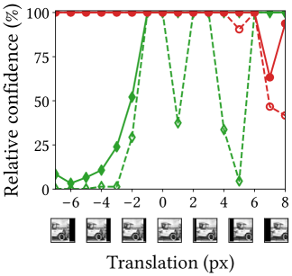
Figure E.3: Spatial smoothing improves the confidence when the predictions are incorrect. We define relative confidence (See Eq. 148), and measure the metric of ResNet-18 on CIFAR-10-P.

To represent the NN reliability appropreately, we propose relative confidence ($\uparrow$) as follows:

$$\text{Relative confidence}=p(y_{\text{true}}|\bm{x},\mathcal{D})\big{/}\,\text{max}\,p(\bm{y}|\bm{x},\mathcal{D})$$ (148)

where $\text{max}\,p(\bm{y}|\bm{x},\mathcal{D})$ is confidence of predictive result and $p(y_{\text{true}}|\bm{x},\mathcal{D})$ is probability of the result for true label. It is 1 when NN classifies the image correctly, and less than 1 when NN classifies it incorrectly. Therefore, relative confidence is a metric that indicates the overconfidence of a prediction when NN’s prediction is incorrect.

Figure E.3 shows a qualitative example of consistency on CIFAR-10-P by using relative confidence. This figure suggests that spatial smoothing improves consistency of both deterministic and Bayesian NN.

E.2 Semantic Segmentation

Table E.4 shows the performance of U-Net on the CamVid dataset. This table indicates that spatial smoothing improves accuracy, uncertainty, and consistency of deterministic and Bayesian NNs. In addition, temporal smoothing leads to significant improvement in efficiency of ensemble size, accuracy, uncertainty, and consistency by exploiting temporal information. Moreover, temporal smoothing requires only one ensemble to achieve high predictive performance, since it cooperates with the temporally previous predictions. We obtain the best predictive and computational performance by using both temporal smoothing and spatial smoothing.

Appendix F Probs Play an Important Role in Spatial Smoothing

As discussed in Section 2.1, we take the perspective that each point in feature map is a prediction for binary classification by deriving the Bernoulli distributions from the feature map by using Prob. It is in contrast to previous works known as sampling-free BNNs (Hernández-Lobato & Adams, 2015; Wang et al., 2016; Wu et al., 2019) attempting to approximate the distribution of feature map with one Gaussian distribution. We do not use any assumptions on the distribution of feature map, and exactly represent the Bernoulli distributions and their averages. However, sampling-free BNNs are error-prone because there is no guarantee that feature maps will follow a Gaussian distribution.

This Prob plays an important role in spatial smoothing. CNNs, such as VGG, ResNet, and ResNeXt, generally use post-activation arrangement. In other words, their stages end with BatchNorm and ReLU. Therefore, spatial smoothing layers $\texttt{Smooth}(\bm{z})=\texttt{Blur}\circ\texttt{Prob}(\bm{z})$ in CNNs cooperates with BatchNorm and ReLU as follows:

$$\texttt{Prob}(\bm{z}) =\texttt{ReLU}\circ\texttt{tanh}_{\tau}\circ\texttt{ReLU}\circ\texttt{BatchNorm}\,(\bm{z})$$ (149)

$$=\texttt{ReLU}\circ\texttt{tanh}_{\tau}\circ\texttt{BatchNorm}\,(\bm{z})$$ (150)

since ReLU and $\texttt{tanh}_{\tau}$ are commutative, and $\texttt{ReLU}\circ\texttt{ReLU}$ is ReLU. This Prob is trainable and is a general form of Eq. 7. If we only use Blur as spatial smoothing, the activations BatchNorm–ReLU play the role of Prob.

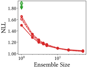
Figure F.1: Blur alone harms the predictive performance, although Prob + Blur improves it. We provide NLL of pre-activation VGG-16 on CIFAR-100.

In order to analyze the roles of Prob and Blur more precisely, we measure the predictive performance of the model that does not use the post-activation. Figure F.1 shows NLL of pre-activation VGG-16 on CIFAR-100. The result shows that Blur with Prob improves the performance, but Blur alone does not. In fact, contrary to Zhang (2019), blur degrades the predictive performance since it results in loss of information. We also measure the performance of VGG-19, ResNet-18, ResNet-50, and BlurPool (Zhang, 2019) with pre-activation, and observe the same phenomenon. In addition, BatchNorm–ReLU in front of GAP significantly improves the performance of pre-activation ResNet. This observation also supports the claim.

As mentioned in Section C.2, pre-activation is a special case of spatial smoothing. Therefore, the performance improvement of pre-activation by spatial smoothing is marginal compared to that of post-activation.

References

- Antoran et al. (2020) Antoran, J., Allingham, J., and Hernández-Lobato, J. M. Depth uncertainty in neural networks. In Advances in Neural Information Processing Systems, 2020.
- Azulay & Weiss (2019) Azulay, A. and Weiss, Y. Why do deep convolutional networks generalize so poorly to small image transformations? Journal of Machine Learning Research, 2019.
- Brostow et al. (2008) Brostow, G. J., Shotton, J., Fauqueur, J., and Cipolla, R. Segmentation and recognition using structure from motion point clouds. In European Conference on Computer Vision, 2008.
- Dosovitskiy et al. (2021) Dosovitskiy, A., Beyer, L., Kolesnikov, A., Weissenborn, D., Zhai, X., Unterthiner, T., Dehghani, M., Minderer, M., Heigold, G., Gelly, S., et al. An image is worth 16x16 words: Transformers for image recognition at scale. In International Conference on Learning Representations, 2021.
- Dusenberry et al. (2020) Dusenberry, M., Jerfel, G., Wen, Y., Ma, Y., Snoek, J., Heller, K., Lakshminarayanan, B., and Tran, D. Efficient and scalable bayesian neural nets with rank-1 factors. In International Conference on Machine Learning, 2020.
- Engstrom et al. (2019) Engstrom, L., Tran, B., Tsipras, D., Schmidt, L., and Madry, A. Exploring the landscape of spatial robustness. In International Conference on Machine Learning, 2019.
- Foret et al. (2021) Foret, P., Kleiner, A., Mobahi, H., and Neyshabur, B. Sharpness-aware minimization for efficiently improving generalization. In International Conference on Learning Representations, 2021.
- Fort et al. (2019) Fort, S., Hu, H., and Lakshminarayanan, B. Deep ensembles: A loss landscape perspective. arXiv preprint arXiv:1912.02757, 2019.
- Frankle et al. (2021) Frankle, J., Schwab, D. J., and Morcos, A. S. Training batchnorm and only batchnorm: On the expressive power of random features in cnns. In International Conference on Learning Representations, 2021.
- Gal & Ghahramani (2016) Gal, Y. and Ghahramani, Z. Dropout as a bayesian approximation: Representing model uncertainty in deep learning. In International Conference on Machine Learning, 2016.
- Ghorbani et al. (2019) Ghorbani, B., Krishnan, S., and Xiao, Y. An investigation into neural net optimization via hessian eigenvalue density. In International Conference on Machine Learning, 2019.
- Goodfellow et al. (2015) Goodfellow, I. J., Shlens, J., and Szegedy, C. Explaining and harnessing adversarial examples. In International Conference on Learning Representations, 2015.
- Goyal et al. (2017) Goyal, P., Dollár, P., Girshick, R., Noordhuis, P., Wesolowski, L., Kyrola, A., Tulloch, A., Jia, Y., and He, K. Accurate, large minibatch sgd: Training imagenet in 1 hour. arXiv preprint arXiv:1706.02677, 2017.
- Guo et al. (2017) Guo, C., Pleiss, G., Sun, Y., and Weinberger, K. Q. On calibration of modern neural networks. In International Conference on Machine Learning, 2017.
- He et al. (2016a) He, K., Zhang, X., Ren, S., and Sun, J. Deep residual learning for image recognition. In Proceedings of the IEEE Conference on Computer Vision and Pattern Recognition, 2016a.
- He et al. (2016b) He, K., Zhang, X., Ren, S., and Sun, J. Identity mappings in deep residual networks. In European Conference on Computer Vision, 2016b.
- Hendrycks & Dietterich (2019) Hendrycks, D. and Dietterich, T. Benchmarking neural network robustness to common corruptions and perturbations. In International Conference on Learning Representations, 2019.
- Hernández-Lobato & Adams (2015) Hernández-Lobato, J. M. and Adams, R. Probabilistic backpropagation for scalable learning of bayesian neural networks. In International Conference on Machine Learning, 2015.
- Hoffer et al. (2020) Hoffer, E., Ben-Nun, T., Hubara, I., Giladi, N., Hoefler, T., and Soudry, D. Augment your batch: Improving generalization through instance repetition. In Proceedings of the IEEE Conference on Computer Vision and Pattern Recognition, 2020.
- Kendall & Gal (2017) Kendall, A. and Gal, Y. What uncertainties do we need in bayesian deep learning for computer vision? In Advances in Neural Information Processing Systems, 2017.
- Kendall et al. (2017) Kendall, A., Badrinarayanan, V., and Cipolla, R. Bayesian segnet: Model uncertainty in deep convolutional encoder-decoder architectures for scene understanding. In BMVC, 2017.
- Keskar et al. (2017) Keskar, N. S., Mudigere, D., Nocedal, J., Smelyanskiy, M., and Tang, P. T. P. On large-batch training for deep learning: Generalization gap and sharp minima. In International Conference on Learning Representations, 2017.
- Krizhevsky & Hinton (2010) Krizhevsky, A. and Hinton, G. Convolutional deep belief networks on cifar-10. Unpublished manuscript, 2010.
- Krizhevsky et al. (2009) Krizhevsky, A., Hinton, G., et al. Learning multiple layers of features from tiny images. 2009.
- Lakshminarayanan et al. (2017) Lakshminarayanan, B., Pritzel, A., and Blundell, C. Simple and scalable predictive uncertainty estimation using deep ensembles. In Advances in Neural Information Processing Systems, 2017.
- Li et al. (2018) Li, H., Xu, Z., Taylor, G., Studer, C., and Goldstein, T. Visualizing the loss landscape of neural nets. In Advances in Neural Information Processing Systems, 2018.
- Lin et al. (2014) Lin, M., Chen, Q., and Yan, S. Network in network. In International Conference on Learning Representations, 2014.
- Loquercio et al. (2020) Loquercio, A., Segu, M., and Scaramuzza, D. A general framework for uncertainty estimation in deep learning. IEEE Robotics and Automation Letters, 2020.
- Madry et al. (2018) Madry, A., Makelov, A., Schmidt, L., Tsipras, D., and Vladu, A. Towards deep learning models resistant to adversarial attacks. In International Conference on Learning Representations, 2018.
- Malinin & Gales (2018) Malinin, A. and Gales, M. Predictive uncertainty estimation via prior networks. In Advances in Neural Information Processing Systems, 2018.
- Ovadia et al. (2019) Ovadia, Y., Fertig, E., Ren, J., Nado, Z., Sculley, D., Nowozin, S., Dillon, J., Lakshminarayanan, B., and Snoek, J. Can you trust your model’s uncertainty? evaluating predictive uncertainty under dataset shift. In Advances in Neural Information Processing Systems, 2019.
- Park & Kim (2022) Park, N. and Kim, S. How do vision transformers work? In International Conference on Learning Representations, 2022.
- Park et al. (2021) Park, N., Lee, T., and Kim, S. Vector quantized bayesian neural network inference for data streams. In Proceedings of the AAAI Conference on Artificial Intelligence, 2021.
- Paszke et al. (2019) Paszke, A., Gross, S., Massa, F., Lerer, A., Bradbury, J., Chanan, G., Killeen, T., Lin, Z., Gimelshein, N., Antiga, L., et al. Pytorch: An imperative style, high-performance deep learning library. In Advances in Neural Information Processing Systems, 2019.
- Postels et al. (2019) Postels, J., Ferroni, F., Coskun, H., Navab, N., and Tombari, F. Sampling-free epistemic uncertainty estimation using approximated variance propagation. In International Conference on Computer Vision, 2019.
- Ronneberger et al. (2015) Ronneberger, O., Fischer, P., and Brox, T. U-net: Convolutional networks for biomedical image segmentation. In International Conference on Medical image computing and computer-assisted intervention, 2015.
- Russakovsky et al. (2015) Russakovsky, O., Deng, J., Su, H., Krause, J., Satheesh, S., Ma, S., Huang, Z., Karpathy, A., Khosla, A., Bernstein, M., Berg, A. C., and Fei-Fei, L. ImageNet Large Scale Visual Recognition Challenge. International Journal of Computer Vision, 2015.
- Sandler et al. (2018) Sandler, M., Howard, A., Zhu, M., Zhmoginov, A., and Chen, L.-C. Mobilenetv2: Inverted residuals and linear bottlenecks. In Proceedings of the IEEE Conference on Computer Vision and Pattern Recognition, 2018.
- Santurkar et al. (2018) Santurkar, S., Tsipras, D., Ilyas, A., and Madry, A. How does batch normalization help optimization? In Advances in Neural Information Processing Systems, 2018.
- Shao et al. (2021) Shao, R., Shi, Z., Yi, J., Chen, P.-Y., and Hsieh, C.-J. On the adversarial robustness of visual transformers. arXiv preprint arXiv:2103.15670, 2021.
- Simonyan & Zisserman (2015) Simonyan, K. and Zisserman, A. Very deep convolutional networks for large-scale image recognition. In International Conference on Learning Representations, 2015.
- Sinha et al. (2020) Sinha, S., Garg, A., and Larochelle, H. Curriculum by smoothing. In Advances in Neural Information Processing Systems, 2020.
- Vasconcelos et al. (2020) Vasconcelos, C., Larochelle, H., Dumoulin, V., Roux, N. L., and Goroshin, R. An effective anti-aliasing approach for residual networks. arXiv preprint arXiv:2011.10675, 2020.
- Vaswani et al. (2017) Vaswani, A., Shazeer, N., Parmar, N., Uszkoreit, J., Jones, L., Gomez, A. N., Kaiser, Ł., and Polosukhin, I. Attention is all you need. In Advances in Neural Information Processing Systems, 2017.
- Veit et al. (2016) Veit, A., Wilber, M. J., and Belongie, S. Residual networks behave like ensembles of relatively shallow networks. In Advances in Neural Information Processing Systems, 2016.
- Wang et al. (2016) Wang, H., Shi, X., and Yeung, D.-Y. Natural-parameter networks: A class of probabilistic neural networks. In Advances in Neural Information Processing Systems, 2016.
- Wang et al. (2022) Wang, P., Zheng, W., Chen, T., and Wang, Z. Scaling the depth of vision transformers via the fourier domain analysis. In International Conference on Learning Representations, 2022.
- Wang et al. (2018) Wang, X., Girshick, R., Gupta, A., and He, K. Non-local neural networks. In Proceedings of the IEEE Conference on Computer Vision and Pattern Recognition, 2018.
- Wen et al. (2020) Wen, Y., Tran, D., and Ba, J. Batchensemble: an alternative approach to efficient ensemble and lifelong learning. In International Conference on Learning Representations, 2020.
- Wilson & Izmailov (2020) Wilson, A. G. and Izmailov, P. Bayesian deep learning and a probabilistic perspective of generalization. In International Conference on Machine Learning, 2020.
- Wu et al. (2019) Wu, A., Nowozin, S., Meeds, E., Turner, R. E., Hernández-Lobato, J. M., and Gaunt, A. L. Deterministic variational inference for robust bayesian neural networks. In International Conference on Learning Representations, 2019.
- Xie et al. (2017) Xie, S., Girshick, R., Dollár, P., Tu, Z., and He, K. Aggregated residual transformations for deep neural networks. In Proceedings of the IEEE Conference on Computer Vision and Pattern Recognition, 2017.
- Yao et al. (2020) Yao, Z., Gholami, A., Keutzer, K., and Mahoney, M. W. Pyhessian: Neural networks through the lens of the hessian. In 2020 IEEE International Conference on Big Data (Big Data), 2020.
- Yoon et al. (2018) Yoon, J., Kim, T., Dia, O., Kim, S., Bengio, Y., and Ahn, S. Bayesian model-agnostic meta-learning. In Advances in Neural Information Processing Systems, 2018.
- Zagoruyko & Komodakis (2016) Zagoruyko, S. and Komodakis, N. Wide residual networks. In BMVC, 2016.
- Zhang (2019) Zhang, R. Making convolutional networks shift-invariant again. In International Conference on Machine Learning, 2019.
- Zhou et al. (2016) Zhou, B., Khosla, A., Lapedriza, A., Oliva, A., and Torralba, A. Learning deep features for discriminative localization. In Proceedings of the IEEE Conference on Computer Vision and Pattern Recognition, 2016.
- Zou et al. (2020) Zou, X., Xiao, F., Yu, Z., and Lee, Y. J. Delving deeper into anti-aliasing in convnets. In BMVC, 2020.