Predict then Interpolate: A Simple Algorithm to Learn Stable Classifiers

Abstract

We propose Predict then Interpolate (pi), a simple algorithm for learning correlations that are stable across environments. The algorithm follows from the intuition that when using a classifier trained on one environment to make predictions on examples from another environment, its mistakes are informative as to which correlations are unstable. In this work, we prove that by interpolating the distributions of the correct predictions and the wrong predictions, we can uncover an oracle distribution where the unstable correlation vanishes. Since the oracle interpolation coefficients are not accessible, we use group distributionally robust optimization to minimize the worst-case risk across all such interpolations. We evaluate our method on both text classification and image classification. Empirical results demonstrate that our algorithm is able to learn robust classifiers (outperforms IRM by 23.85% on synthetic environments and 12.41% on natural environments). Our code and data are available at https://github.com/YujiaBao/Predict-then-Interpolate.

1 Introduction

Distributionally robust optimization (DRO) alleviates model biases by minimizing the worst-case risk over a set of human-defined groups. However, in order to construct these groups, humans must identify and annotate these biases, a process as expensive as annotating the label itself (Ben-Tal et al., 2013; Duchi & Namkoong, 2018; Sagawa et al., 2019). In this paper we propose a simple algorithm to create groups that are informative of these biases, and use these groups to train stable classifiers.

Our algorithm operates on data split among multiple environments, across which correlations between bias features and the label may vary. Instead of handcrafting environments based on explicit, task-dependent biases, these environments can be determined by generic information that is easy to collect (Peters et al., 2015). For example, environments can represent data collection circumstances, like location and time. Our goal is to learn correlations that are stable across these environments.

Given these environments, one could directly use them as groups for DRO. Doing so would optimize the worst-case risk over all interpolations of the training environments. However, if the unstable (bias) features are positively and differentially correlated with the label in all training environments, the unstable correlation will be positive in any of their interpolations. DRO, optimizing for the best worst-case performance, will inevitably exploit these unstable features, and we fail to learn a stable classifier.

In this work, we propose Predict then Interpolate (pi), a simple recipe for creating groups whose interpolation yields a distribution with only stable correlations. Our idea follows from the intuition that when using a classifier trained on one environment to make predictions on examples from a different environment, its mistakes are informative of the unstable correlations. In fact, we can prove that if the unstable features and the label are positively correlated across all environments, the same correlation flips to negative in the set of mistakes. Therefore, by interpolating the distributions of correct and incorrect predictions, we can uncover an “oracle” distribution in which only stable features are correlated with the label. Although the oracle interpolation coefficients are not accessible, we can minimize the worst-case risk over all interpolations, providing an upper bound of the risk on the oracle distribution.

Our learning paradigm consists of three steps. First, we train an individual classifier for each environment to estimate the conditional distribution of the label given the input. These classifiers are biased, as they may rely on any correlations in the dataset. Next, we apply each environment’s classifier to partition all other environments, based on prediction correctness. Finally, we obtain our robust classifier by minimizing the worst-case risk over all interpolations of the partitions.

Empirically, we evaluate our approach on both synthetic and real-world environments. First, we simulate unstable correlations in synthetic environments by appending spurious features. Our results in both digit classification and aspect-level sentiment classification demonstrate that our method delivers significant performance gain (23.85% absolute accuracy) over invariant risk minimization (IRM), approaching oracle performance. Quantitative analyses confirm that our method generates partitions with opposite unstable correlations. Next, we applied our approach on natural environments defined by an existing attribute of the input. Our experiments on CelebA and ASK2ME showed that directly applying DRO on environments improves robust accuracy for known attributes, but this robustness doesn’t generalize equally across other attributes that are unknown during train time. On the other hand, by creating partitions with opposite unstable correlations, our method is able to improve average worst-group accuracy by 12.41% compared to IRM.

2 Related work

Removing known biases:

Large scale datasets are fraught with biases. For instance, in face recognition (Liu et al., 2015a), spurious associations may exist between different face attributes (e.g. hair color) and demographic information (e.g. ethnicity) (Buolamwini & Gebru, 2018). Furthermore, in natural language inference (Bowman et al., 2015), the entailment label can often be predicted from lexical overlap of the two inputs (McCoy et al., 2019). Finally, in molecular property prediction (Wu et al., 2018; Mayr et al., 2018), performance varies significantly across different scaffolds (Yang et al., 2019).

Many approaches have been proposed to mitigate biases when they are known beforehand. Examples include adversarial training to remove biases from representations (Belinkov et al., 2019; Stacey et al., 2020), re-weighting training examples (Schuster et al., 2019), and combining a biased model and the base model’s predictions using a product of experts (Hinton, 2002; Clark et al., 2019; He et al., 2019; Mahabadi et al., 2020). These models are typically designed for a specific type of bias and thus require extra domain knowledge to generalize to new tasks.

Group DRO is another attractive framework since it allows explicit modeling of the distribution family that we want to optimize over. Previous work (Hu et al., 2018; Oren et al., 2019; Sagawa* et al., 2020) has shown the effectiveness of group DRO to train un-biased models. In these models, the groups are specified by human based on the knowledge of the bias attributes. Our work differs from them as we create groups using trained models. This allows us to apply group DRO when we don’t have annotations for the bias attributes. Moreover, when the bias attributes are available, we can further refine our groups to reduce unknown biases.

Removing unknown biases:

Determining dataset biases is time-consuming and often requires task-specific expert knowledge (Zellers et al., 2019; Sakaguchi et al., 2020). Thus, there are two lines of work that aim to build robust models without explicitly knowing the type of bias. The first assumes that weak models, which have limited capacity (Sanh et al., 2021) or are under-trained (Utama et al., 2020), are more prone to rely on shallow heuristics and rediscover previously human-identified dataset biases. By learning from the weak models’ mistakes, we can obtain a more robust model. While these methods show empirical benefits on some NLP tasks, the extent to which their assumption holds is unclear. In fact, recent work (Sagawa et al., 2020) shows that over-parametrization may actually exacerbate unstable correlations for image classification.

The second line of work assumes that the training data are collected from separate environments, across which unstable features exhibit different correlations with the label (Peters et al., 2016; Krueger et al., 2020; Chang et al., 2020; Jin et al., 2020; Ahuja et al., 2020; Arjovsky et al., 2019). Invariant risk minimization (Arjovsky et al., 2019), a representative method along this line, learns representations that are simultaneously optimal across all environments. However, since this representation is trained across all environments, it can easily degenerate in real-world applications (Gulrajani & Lopez-Paz, 2020). One can consider an extreme case where the learned representation directly encodes the one-hot embedding of the label. While this learned representation is stable (invariant) according to the definition, the model can utilize any unstable features to generate this representation. We have no guarantee on how the model would generalize when the unstable correlations vanish.

Our algorithm instead decomposes the problem of learning stable classifiers into two parts: finding unstable features and training a robust model. By constraining the classifiers to be environment-specific in the first part, we are able to construct an oracle distribution where the unstable features are not correlated with the label. Our model then directly optimizes an upper bound of the risk on this oracle distribution. Empirically, we demonstrate that our method is able to eliminate biases not given during training on multiple real-world applications.

3 Method

We consider the standard setting (Arjovsky et al., 2019) where the training data are comprised of $n$ environments $\mathcal{E}=\{E_{1},\ldots,E_{n}\}$. For each environment $E_{i}$, we have input-label pairs $(x,y)\overset{\text{iid}}{\sim}P_{i}$. Our goal is to learn correlations that are stable across these environments (Woodward, 2005) so that the model can generalize to a new test environment $E_{\text{test}}$ that has the same stable correlations.

3.1 Algorithm

Our intuition follows from a simple question.

What happens if we apply a classifier $f_{i}$ trained on environment $E_{i}$ to a different environment $E_{j}$?

Suppose we have enough data in $E_{i}$ and the classifier $f_{i}$ is able to perfectly fit the underlying conditional $P_{i}(y|x)$. Since $E_{i}$ and $E_{j}$ follow different distributions, the classifier $f_{i}$ will make mistakes on $E_{j}$. These mistakes are natural products of the unstable correlation: if the correlation of the unstable feature is higher in $E_{i}$ than in $E_{j}$, the classifier $f_{i}$ will overuse this feature when making predictions in $E_{j}$.

In fact, we can show that under certain conditions, the unstable correlation within the subset of wrong predictions is opposite of that within the subset of correct predictions (Section 3.3). By interpolating between these two subsets, we can uncover an oracle distribution where the label is not correlated with the unstable feature. Since this interpolation coefficient is not accessible in practice, we adopt group DRO to minimize the worst-case risk over all interpolations of these subsets. This provides us an upper bound of the risk on the oracle distribution.

Concretely, our approach has three successive stages.

Stage 1:

For each environment $E_{i}$, train an environment specific classifier $f_{i}$.

Stage 2:

For each pair of environments $E_{i}$ and $E_{j}$, use the trained classifier $f_{i}$ to partition $E_{j}$ into two sets

$$E_{j}=E_{j}^{i\checkmark}\cup E_{j}^{i\times}$$

where $E_{j}^{i\checkmark}$ contains examples that $f_{i}$ predicted correctly and $E_{j}^{i\times}$ contains those predicted incorrectly.

Stage 3:

Train the final model $f$ by minimizing the worst-case risk over the set of all interpolations $\mathcal{Q}$:

$$\mathcal{Q}=\left\{\sum_{i\neq j}\lambda_{j}^{i\checkmark}P_{j}^{i\checkmark}+\lambda_{j}^{i\times}P_{j}^{i\times}:\sum_{i\neq j}\lambda_{j}^{i\checkmark}+\lambda_{j}^{i\times}=1\right\},$$

where $P_{j}^{i\checkmark}$ and $P_{j}^{i\times}$ are the empirical distributions of $E_{j}^{i\checkmark}$ and $E_{j}^{i\times}$. Because the optimum value of a linear program must occur at a vertex, the worst-case risk over $\mathcal{Q}$ is equivalent to the maximum expected risk across all groups. This allows us to formulate the objective as a min-max problem:

$$\min_{f}\max_{P\in\mathcal{P}}\mathbb{E}_{(x,y)\sim P}[\mathcal{L}(x,y;f)],$$

where $\mathcal{L}(x,y;f)$ is the loss of the model $f$ and $\mathcal{P}$ is the set of distributions $\{P_{j}^{i\checkmark}\}_{i\neq j}\cup\{P_{j}^{i\times}\}_{i\neq j}$.

Extensions of the algorithm:

For regression tasks, we can set a threshold on the mean square error to partition environments. We can also apply the first two stages multiple times, treating new partitions as different environments, to iteratively refine the groups. In this work, we focus on the basic setting and leave the rest for future work.

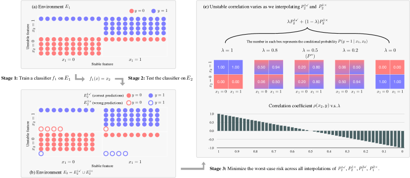
Figure 1: Illustration of our algorithm on the toy example. The label $y$ agrees with the stable feature $x_{1}$ with probability $0.8$ on both environments. For the unstable feature $x_{2}$, the probability of $x_{2}=y$ is $1.0$ in $E_{1}$ and $0.9$ in $E_{2}$. Stage 1: We train a classifier $f_{1}$ on $E_{1}$. It learns to make predictions solely based on the unstable feature $x_{2}$. Stage 2: We use $f_{1}$ to partition $E_{2}$ based on the prediction correctness. While the correlation of $x_{2}$ is positive for both $E_{1}$ and $E_{2}$, it flips to negative in set of wrong predictions $E_{2}^{1\times}$. Stage 3: Interpolating $P_{2}^{1\checkmark}$ and $P_{2}^{1\times}$ allows us to uncover an oracle distribution $P^{*}$ where the unstable feature $x_{2}$ is not correlated with the label. Note that here we only illustrate how to partition $E_{2}$ using $f_{1}$. In our algorithm, we also use the classifier $f_{2}$ (trained on $E_{2}$) to partition $E_{1}$, and the final model $f$ is obtained by minimizing the worst-case risk over all interpolations of $P_{1}^{2\checkmark},P_{1}^{2\times},P_{2}^{1\checkmark}P_{2}^{1\times}$.

3.2 A toy example

To understand the behavior of the algorithm, let’s consider a simple example with two environments $E_{1}$ and $E_{2}$ (Figure 1). For each environment, the data are generated by the following process.

• First, sample the feature $x_{1}\in\{0,1\}$ which takes the value $1$ with probability $0.5$. This is our stable feature.

• Next, sample the observed noisy label $y\in\{0,1\}$ by flipping the value of $x_{1}$ with probability $0.2$.

• Finally, for each environment $E_{i}$, sample the unstable feature $x_{2}\in\{0,1\}$ by flipping the value of $y$ with probability $\eta_{i}$. Let $\eta_{1}=0$ and $\eta_{2}=0.1$.

Our goal is to learn a classifier that only uses feature $x_{1}$ to predict $y$. Since the unstable feature $x_{2}$ is positively correlated with the label across both environments, directly treating the environments as groups and applying group DRO will also exploit this correlation during training.

Let’s take a step back and consider a classifier $f_{1}$ that is trained only on $E_{1}$. Since $x_{2}$ is identical to $y$ and $x_{1}$ differs from $y$ with probability $0.2$, $f_{1}$ simply learns to ignore $x_{1}$ and predict $y$ as $x_{2}$ (Figure 1a). When we apply $f_{1}$ to the other environment $E_{2}$, it will make mistakes on examples where $x_{2}$ is flipped from $y$. Moreover, we can check that the correlation coefficient between the unstable feature $x_{2}$ and $y$ is $1$ in the set of correct predictions $E_{2}^{1\checkmark}$ and it flips to $-1$ in the set of mistakes $E_{2}^{1\times}$ (Figure 1b). In this toy example, the oracle distribution $P^{*}$, where the correlation between $x_{2}$ and $y$ is $0$, can be obtained by simply averaging the empirical distribution of the two subsets (Figure 1c):

$$P^{*}(x_{1},x_{2},y)=0.5P_{2}^{1\checkmark}(x_{1},x_{2},y)+0.5P_{2}^{1\times}(x_{1},x_{2},y).$$

We can also verify that the optimal solution that minimize the worst-case risk across $E_{2}^{1\checkmark}$ and $E_{2}^{1\times}$ is to predict $y$ only using $x_{1}$. (Appendix A).

Remark 1:

In the algorithm, we also use the classifier $f_{2}$ trained on $E_{2}$ to partition $E_{1}$. The final model $f$ is obtained by minimizing the worst-case risk over $P_{1}^{2\checkmark},P_{1}^{2\times},P_{2}^{1\checkmark},P_{2}^{1\times}$.

Remark 2:

Our algorithm optimizes an upper bound of the risk on the oracle distribution. In general, it doesn’t guarantee that the unstable correlation is not utilized by the model when the worst-case performance is not achieved at the oracle distribution.

3.3 Theoretical analysis

In the previous example, we have seen that the unstable correlation flips in the set of mistakes $E_{2}^{1\times}$ compared to the set of correct predictions $E_{2}^{1\checkmark}$. Here, we would like to investigate how this property holds in general. We focus our analysis on binary classification tasks where $y\in\{0,1\}$. Let $x_{1}$ be the stable feature and $x_{2}$ be unstable feature that has various correlations across environments. We use capital letters $X_{1},X_{2},Y$ to represent random variables and use lowercase letters $x_{1},x_{2},y$ to denote their specific values.

Proposition 1.

For a pair of environments $E_{i}$ and $E_{j}$, assuming that the classifier $f_{i}$ is able to learn the true conditional $P_{i}(Y\mid X_{1},X_{2})$, we can write the joint distribution $P_{j}$ of $E_{j}$ as the mixture of $P_{j}^{i\checkmark}$ and $P_{j}^{i\times}$:

$$P_{j}(x_{1},x_{2},y)=\alpha_{j}^{i}P_{j}^{i\checkmark}(x_{1},x_{2},y)+(1-\alpha_{j}^{i})P_{j}^{i\times}(x_{1},x_{2},y),$$

where $\alpha_{j}^{i}=\sum_{x_{1},x_{2},y}P_{j}(x_{1},x_{2},y)\cdot P_{i}(y\mid x_{1},x_{2})$ and

$$P_{j}^{i\checkmark}(x_{1},x_{2},y) \propto P_{j}(x_{1},x_{2},y)\cdot P_{i}(y\mid x_{1},x_{2}),$$

$$P_{j}^{i\times}(x_{1},x_{2},y) \propto P_{j}(x_{1},x_{2},y)\cdot P_{i}(1-y\mid x_{1},x_{2}).$$

Intuitively, when partitioning the environment $E_{j}$, we are scaling its joint distribution based on the conditional on $E_{i}$.

Two degenerate cases:

From Proposition 1, we see that the algorithm degenerates when $\alpha_{j}^{i}=0$ (predictions of $f_{i}$ are all wrong) or $\alpha_{j}^{i}=1$ (predictions of $f_{i}$ are all correct). The first case occurs when the unstable correlation is flipped between $P_{i}$ and $P_{j}$. One may think about setting $\eta_{1}=0$ and $\eta_{2}=1$ in the toy example. In this case, we can obtain the oracle distribution by directly interpolating $P_{i}$ and $P_{j}$. The second case implies that the conditional is the same across the environments: $P_{i}(Y\mid X_{1},X_{2})=P_{j}(Y\mid X_{1},X_{2})$. Since $x_{2}$ is the unstable feature, this equality holds when the conditional mutual information between $X_{2}$ and $Y$ is zero given $X_{1}$, i.e., $P_{i}(Y\mid X_{1},X_{2})=P_{i}(Y\mid X_{1})$. In this case, $f_{i}$ already ignores the unstable feature $x_{2}$.

To carryout the following analysis, we assume that the marginal distribution of $Y$ is uniform in all joint distributions, i.e., $f_{i}$ performs equally well on different labels.

Theorem 1.

Suppose $X_{2}$ is independent of $X_{1}$ given $Y$. For any environment pair $E_{i}$ and $E_{j}$, if $\sum_{y}P_{i}(x_{2}\mid y)=\sum_{y}P_{j}(x_{2}\mid y)$ for any $x_{2}$, then $\mathrm{Cov}(X_{2},Y;P_{i})>\mathrm{Cov}(X_{2},Y;P_{j})$ implies $\mathrm{Cov}(X_{2},Y;P_{j}^{i\times})<0$ and $\mathrm{Cov}(X_{2},Y;P_{i}^{j\times})>0$.

The result follows from the connection between the covariance and the conditional. On one side, the covariance between $x_{2}$ and $Y$ captures the difference of their conditionals: $P(X_{2}\mid Y=1)-P(X_{2}\mid Y=0)$, On the other side, the conditional independence assumption allows us to factorize the joint distribution: $P_{i}(x_{1},x_{2},y)=P_{i}(x_{1},y)P_{i}(x_{2}\mid y)$. Combining them together finishes the proof.

Theorem 1 tells us no matter whether the spurious correlation is positive or negative, we can obtain an oracle distribution $P^{*}$, $\mathrm{Cov}(X_{2},Y;P^{*})=0$ by interpolating across $P_{j}^{i\checkmark}$, $P_{j}^{i\times}$, $P_{i}^{j\checkmark}$, $P_{i}^{j\times}$. By optimizing the worst-case risk across all interpolations, our final model $f$ provides an upper bound of the risk on the oracle distribution $P^{*}$.

We also note that the toy example in Section 3.2 is a special case of the assumption in Theorem 1. While many previous work also construct datasets with this assumption (Arjovsky et al., 2019; Choe et al., 2020), it may be too restrictive in practice. In the general case, although we cannot guarantee the sign of the correlation, we can still obtain an upper bound for $\mathrm{Cov}(X_{2},Y;P_{j}^{i\times})$ and a lower bound for $\mathrm{Cov}(X_{2},Y;P_{i}^{j\times})$:

Theorem 2.

For any environment pair $E_{i}$ and $E_{j}$, $\mathrm{Cov}(X_{2},Y;P_{i})>\mathrm{Cov}(X_{2},Y;P_{j})$ implies

$$\mathrm{Cov}(X_{2},Y;P_{j}^{i\times})$$

$$<\frac{1-\alpha_{j}^{i}}{\alpha_{i}^{i}}\mathrm{Cov}(X_{2},Y;P_{i}^{i\checkmark})-\frac{1-\alpha_{j}^{i}}{\alpha_{j}^{i}}\mathrm{Cov}(X_{2},Y;P_{j}^{i\checkmark})$$

$$\mathrm{Cov}(X_{2},Y;P_{i}^{j\times})$$

$$>\frac{1-\alpha_{i}^{j}}{\alpha_{j}^{j}}\mathrm{Cov}(X_{2},Y;P_{j}^{j\checkmark})-\frac{1-\alpha_{i}^{j}}{\alpha_{i}^{j}}\mathrm{Cov}(X_{2},Y;P_{i}^{j\checkmark})$$

where $P_{i}^{i\checkmark}$ is the distribution of the correct predictions when applying $f_{i}$ on $E_{i}$.

Intuitively, if the correlation is stronger in $E_{i}$, then the classifier $f_{i}$ will overuse this correlation and make mistakes on $E_{j}$ when this stronger correlation doesn’t hold. Conversely, the classifier $f_{j}$ will underuse this correlation and make mistakes on $E_{i}$ when the correlation is stronger.

	erm		dro		irm		rgm		pi (ours)		oracle
$P_{\text{val}}=P_{\text{test}}$?	✓	$\times$	✓	$\times$	✓	$\times$	✓	$\times$	✓	$\times$	✓	$\times$
MNIST	26.15	14.25	32.51	21.06	45.41	13.13	42.49	15.33	$\bm{69.44}$	$\bm{69.68}$	71.40	71.60
Beer Look	64.63	60.96	64.53	62.75	65.83	63.31	66.31	61.51	$\bm{78.09}$	$\bm{70.66}$	80.32	73.51
Beer Aroma	55.25	51.99	57.08	53.39	60.25	53.25	66.33	57.91	$\bm{77.01}$	$\bm{67.35}$	77.34	69.99
Beer Palate	49.01	46.69	47.72	46.35	66.45	44.09	68.77	44.81	$\bm{74.14}$	$\bm{61.51}$	74.89	66.33

Table 1: Accuracy of different methods on image classification (majority baseline 10%) and aspect-level sentiment classification (majority baseline 50%). All methods are tuned based on a held-out validation set. We consider two validation settings: 1) sample the validation set from the testing environment ($P_{\text{val}}=P_{\text{test}}$); 2) sample the validation set from the training environment.

4 Experimental setup

4.1 Datasets and Settings

Synthetic environments:

To assess the empirical behavior of our algorithm, we start with controlled experiments where we can simulate spurious correlation. We consider two standard datasets: MNIST (LeCun et al., 1998) and BeerReview (McAuley et al., 2012).

For MNIST, we adopt Arjovsky et al. (2019)’s approach for generating spurious correlation and extend it to a more challenging multi-class problem. For each image, we sample $y$, which takes on the same value as its numeric digit with 0.75 probability and a uniformly random other digit with the remaining probability. The spurious feature in sampled in a similar way: it takes on the same value as $y$ with $\eta$ probability and a uniformly random other value with the remaining probability. We color the image according to the value of the spurious feature. We set $\eta$ to $0.9$ and $0.8$ respectively for the training environments $E_{1}$ and $E_{2}$. In the testing environment, $\eta$ is set to $0.1$.

For BeerReview, we consider three aspect-level sentiment classification tasks: look, aroma and palate (Lei et al., 2016; Bao et al., 2018). For each review, we append an artificial token (art_pos or art_neg) that is spuriously correlated with the binary sentiment label (pos or neg). The artificial token agrees with the sentiment label with probability $0.9$ in environment $E_{1}$ and with probability $0.8$ in environment $E_{2}$. In the testing environment, the probability reduces to $0.1$. Unlike MNIST, here we do not inject artificial label noise to the datasets.

Validation set plays a crucial role when the training distribution is different from the testing distribution (Gulrajani & Lopez-Paz, 2020). For both datasets, we consider two different validation settings and report their performance separately: 1) sampling the validation set from the training environment; 2) sampling the validation set from the testing environment.

Natural environments:

We also consider a practical setting where environments are naturally defined by some attributes of the input and we want to use them to reduce biases that are unknown during training and validation. We study two datasets: CelebA (Liu et al., 2015b) where the attributes are annotated by human and ASK2ME (Bao et al., 2019) where the attributes are automatically generated by rules.

CelebA is an image classification dataset where each input image (face) is paired with 40 binary attributes. We adopt Sagawa et al. (2019)’s setting and treat hair color ($y\in\{\texttt{blond},\texttt{dark}\}$) as the target task. We use the gender attribute to define the two training environments, $E_{1}$={female} and $E_{2}$={male}. Our goal is to learn a classifier that is robust to other unknown attributes such as wearing_hat. For model selection, we partition the validation data into four groups based on the gender value and the label value: {female, blond}, {female, dark}, {male, blond}, {male, dark}. We use the worst-group accuracy as our validation criteria.

ASK2ME is a text classification dataset where an input text (paper abstract from PubMed) is paired with 17 binary attributes, each indicating the presence of a different disease. The task is to predict whether the input is informative about the risk of cancer for gene mutation carriers, rather than cancer itself (Deng et al., 2019). We define two training environments based on the breast_cancer attribute, $E_{1}$={breast_cancer=0} and $E_{2}$={breast_cancer=1}. We would like to see whether the classifier is able to remove spurious correlations from other diseases that are unknown during training. Similar to CelebA, we compute the worst-group accuracy based on the breast_cancer value and the label value and use it for validation.

At test time, we evaluate the classifier’s prediction robustness on all attributes over a held-out test set. For each attribute, we report the worst-group accuracy and the average-group accuracy.

4.2 Baselines

We compare our algorithm against the following baselines:

ERM: We combine all environments together and apply standard empirical risk minimization.

IRM: Invariant risk minimization (Arjovsky et al., 2019) learns a representation such that the linear classifier on top of this representation is simultaneously optimal across different environments.

RGM: Regret minimization (Jin et al., 2020) simulates unseen environments by using part of the training set as held-out environments. It quantifies the generalization ability in terms of regret, the difference between the losses of two auxiliary predictors trained with and without examples in the current environment.

DRO: We can also apply DRO on groups defined by the environments and the labels. For example, in beer review, we can partition the training data into the four groups: {pos, $E_{1}$}, {neg, $E_{1}$} {pos, $E_{2}$}, {neg, $E_{2}$}. Minimizing the worst-case performance over these human-defined groups has shown success in improving model robustness (Sagawa et al., 2019).

Oracle: In the synthetic environments, we can use the spurious features to define groups and train an oracle DRO model. For example, in beer review, the oracle model will minimize the worst-case risk over the four groups: {pos, art_pos}, {pos, art_neg} {pos, art_pos}, {pos, art_neg}. This helps us analyze the contribution of our algorithm in isolation of the inherent limitations of the task.

For fair comparison, all methods share the same model architecture. Implementation details can be found in Appendix C.2.

	$E_{1}$	$E_{2}$	$E_{2}^{1\checkmark}$	$E_{2}^{1\times}$
MNIST	0.8955	0.7769	0.9961	$-0.1040$
Beer Look	0.8007	0.6006	0.8254	$-0.8030$
Beer Aroma	0.8007	0.6006	0.9165	$-0.9303$
Beer Palate	0.8007	0.6006	0.9394	$-0.9189$

Table 2: Pearson correlation coefficient between the spurious feature and the label across four datasets. While the correlation is positive for both training environments, it flips to negative in the set of wrong predictions $E_{2}^{1\times}$. Interpolating across $E_{2}^{1\checkmark}$ and $E_{2}^{1\times}$ allows us to remove the unstable correlation.

	erm		dro		irm		rgm		pi (ours)
	Worst	Avg	Worst	Avg	Worst	Avg	Worst	Avg	Worst	Avg
Kidney cancer	16.67	66.66	50.00	68.70	33.33	73.07	33.33	71.31	50.00	74.76
Adenocarcinoma	33.33	72.91	77.29	79.23	55.56	78.40	55.56	78.12	80.24	84.74
Lung cancer	44.44	74.76	62.50	74.58	38.89	74.28	50.00	74.75	70.31	78.85
Polyp syndrom	44.44	74.63	77.29	78.79	55.56	76.31	66.67	78.73	69.23	81.28
Hepatobiliary cancer	44.44	73.01	60.00	73.89	55.56	77.19	55.56	76.22	60.00	78.94
Breast cancer	66.49	80.47	75.00	78.84	66.87	80.56	64.38	79.81	80.32	83.12
Average∗	54.80	77.73	67.34	77.58	57.86	79.18	60.81	79.03	74.15	83.15

Table 3: Worst-group and average-group accuracy on ASK2ME text classification. We show the results for the worst 5 attributes (sorted based on ERM) and the given attribute breast_cancer. Average is computed based on the performance across all attributes. See Appendix D for full results.

5 Results

5.1 Synthetic environments

Table 1 summarizes the results on synthetic environments. As we expected, since the signs of the unstable correlation are the same across the training environments, both ERM and DRO exploit this information and fail to generalize when it changes in the testing environment. While IRM and RGM are able to learn stable correlations when we use the testing environment for model selection, their performance quickly drop to that of ERM when the validation data is drawn from the training environment, which also backs up the claim from Gulrajani & Lopez-Paz (2020).

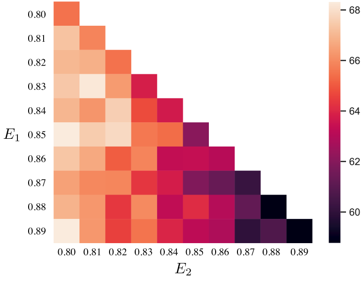
Figure 2: The ability of generalization changes as we vary the gap between the training environments. The x and y axes denote the probabilities that the injected artificial token agrees with the label. Heatmap corresponds to the testing accuracy for Beer Aroma.

Our algorithm obtains substantial gains across four tasks It performs much more stable under different validation settings. Specifically, comparing against the best baseline, our algorithm improves the accuracy by 20.06% when the validation set is drawn from the training environment and 12.97% when it is drawn from the testing environment. Its performance closely matches the oracle model with only 2% difference on average.

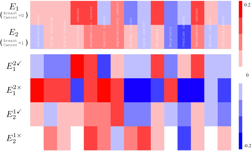
Figure 3: Visualization of the Pearson correlation coefficient between the label and the attribute on ASK2ME. Each column corresponds to a different attribute. We observe that correlations vary for inputs with different breast_cancer value. Our algorithm utilizes this difference to create partitions with opposite correlations (red vs. blue) so that we can uncover an oracle distribution (different for each attribute) by interpolating these partitions.

Why does partitioning the training environments help? To demystify the huge performance gain, we quantitatively analyze the partitions created by our algorithm in Table 2. We see that while the unstable correlation is positive in both training environments, it flips to negative in the set of wrong predictions, confirming our theoretical analysis. In order to perform well across all partitions, our final classifier learns not to rely on the unstable features.

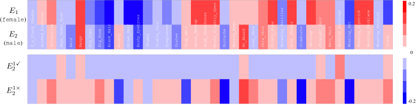
Figure 4: Visualization of the Pearson correlation coefficient between the label (hair color) and other attributes on CelebA. Each column corresponds to a different attribute. Due to the huge difference between the label marginals, $P_{1}(\texttt{blond})=0.24$ vs. $P_{2}(\texttt{blond})=0.02$, classifier $f_{2}$ predicts every example in environment $E_{1}$ as dark. The resulting partition, $E_{1}^{2\times}=\{\texttt{female, blond}\}$ and $E_{1}^{2\checkmark}=\{\texttt{female, dark}\}$, coincides with the human-defined groups in DRO. On the other hand, classifier $f_{1}$ is able to partition environment $E_{2}$ with opposite correlations (red vs. blue).

	erm		dro		irm		rgm		pi (ours)
	Worst	Avg	Worst	Avg	Worst	Avg	Worst	Avg	Worst	Avg
Goatee	0.00	68.26	0.00	70.08	84.80	90.83	91.50	95.66	91.63	94.59
Wearing_Hat	7.69	70.39	46.15	82.28	46.15	77.34	61.54	86.26	53.85	84.56
Chubby	9.52	70.69	61.90	84.63	76.19	82.91	47.62	82.32	71.43	86.59
Wearing_Necktie	25.00	74.52	90.00	91.56	80.00	84.31	35.00	79.32	91.44	92.53
Sideburns	38.46	77.84	84.62	90.69	76.92	84.14	76.92	89.72	91.35	93.75
Gender	46.67	80.14	85.56	90.87	74.44	83.93	70.00	87.73	90.56	91.52
Average∗	60.06	83.63	84.25	90.83	78.51	85.79	82.52	90.95	87.04	91.41

Table 4: Worst-group and average-group accuracy for hair color prediction on CelebA. We show the results for the worst 5 attributes (sorted based on ERM) and the given attribute gender. Average is computed based on the performance across all attributes. See Appendix D for full results.

Do we need different training environments? We study the relation between the diversity of the training environments and the performance of the classifier on the beer review dataset. Specifically, we consider 45 different training environment pairs where we vary the probability that the artificial token agrees with the label from $0.80$ to $0.89$. We observe that the classifier performs better as we reduce the amount of spurious correlations (moving up along the diagonal in Figure 2). The classifier also generalizes better when we increase the gap between the two training environments (moving from right to left in Figure 2). In fact, when the training environments share the same distribution, the notion of stable correlation and unstable correlation is undefined. There is no signal for the algorithm to distinguish between spurious features and features that generalize.

5.2 Natural environments

Table 3 and  4 summarize the results on using natural environments to reduce biases from attributes that are unknown during both training and validation. We observe that directly applying DRO over human-defined groups already surpasses IRM and RGM on the worst-case accuracy averaged across all attributes. In addition, for the given attribute (breast_cancer and gender), DRO achieves nearly 10% more improvements over other baselines. However, this robustness doesn’t generalize equally towards other attributes. By using the environment-specific classifier to create groups with contrasting unstable correlations, our algorithm delivers marked performance improvement over DRO, 6.81% on ASK2ME and 2.79% on CelebA.

How do we reduce bias from unknown attributes? Figure 3 and 4 visualize the correlation between each attribute and the label on ASK2ME and CelebA. We observe that although the signs of the correlation can be the same across the training environments, their magnitude may vary. Our algorithm makes use of this difference to create partitions that have opposite correlations for 13 (out of 15) attributes on ASK2ME and 22 (out of 38) attributes on CelebA. These opposite correlations help the classifier to avoid using unstable features during training.

6 Conclusion

In this paper, we propose a simple algorithm to learn correlations that are stable across environments. Specifically, we propose to use a classifier that is trained on one environment to partition another environment. By interpolating the distributions of its correct predictions and wrong predictions, we can uncover an oracle distribution where the unstable correlation vanishes. Experimental results on synthetic environments and natural environments validate that our algorithm is able to generate paritions with opposite unstable correlations and reduce bias that are unknown during training.

Appendix A A toy example

We would like to show that the optimal solution that minimize the worst-case risk across $E_{2}^{1\checkmark}$ and $E_{2}^{1\times}$ is to predict $Y$ only using $X_{1}$. Consider any classifier $f(Y\mid X_{1},X_{2})$ and its marginal

$$f(Y\mid X_{1})\propto f(X_{1},X_{2}=0,Y)+f(X_{1},X_{2}=1,Y).$$

For any input $(x_{1},x_{2})\in E_{2}^{1\checkmark}$, based on our construction, the distribution $P_{2}^{1\checkmark}(X_{1}=x_{1},X_{2}=x_{2},Y)$ only has mass on one label value $y\in\{0,1\}$. Thus $P_{2}^{1\checkmark}(Y=y\mid X_{1}=x_{1},X_{2}=x_{2})=1$. We can then write the log risk of the classifier $f(Y\mid X_{1},X_{2})$ as

$$-\log\frac{f(x_{1},x_{2},y)}{f(x_{1},x_{2},y)+f(x_{1},x_{2},1-y)}.$$

The log risk of the marginal classifier $f(Y\mid X_{1})$ is defined as

$$-\log\Big{(} (f(x_{1},x_{2},y)+f(x_{1},1-x_{2},y))$$

$$/(f(x_{1},x_{2},y)+f(x_{1},1-x_{2},y)$$

$$\quad+f(x_{1},x_{2},1-y)+f(x_{1},1-x_{2},1-y))\Big{)}.$$

Now suppose $f(Y\mid X_{1},X_{2})$ achieves a lower risk than $f(Y\mid X_{1})$. This implies

$$f(x_{1},x_{2},y)f(x_{1},x_{2},y)+f(x_{1},x_{2},1-y)f(x_{1},x_{2},y)$$

$$\qquad+f(x_{1},x_{2},y)f(x_{1},1-x_{2},y)$$

$$\qquad+f(x_{1},x_{2},1-y)f(x_{1},1-x_{2},y)$$

$$<f(x_{1},x_{2},y)f(x_{1},x_{2},y)+f(x_{1},x_{2},y)f(x_{1},x_{2},1-y)$$

$$\qquad+f(x_{1},x_{2},y)f(x_{1},1-x_{2},y)$$

$$\qquad+f(x_{1},x_{2},y)f(x_{1},1-x_{2},1-y).$$

Note that the first three terms on both side cancel out. We have

$$f(x_{1},x_{2},1-y)f(x_{1},1-x_{2},y)$$

$$\qquad\qquad<f(x_{1},x_{2},y)f(x_{1},1-x_{2},1-y).$$

Now let’s consider an input $(x_{1},1-x_{2})\in E_{2}^{1\times}$. Based on our construction of the partitions, we have $P_{2}^{1\checkmark}(x_{1},x_{2},y)=P_{2}^{1\times}(x_{1},1-x_{2},y)$. The log risk of the marginal classifier on $P_{2}^{1\times}$ is still the same, but the log risk of the classifier $f(Y\mid X_{1},X_{2})$ now becomes

$$-\log\frac{f(x_{1},1-x_{2},y)}{f(x_{1},1-x_{2},y)+f(x_{1},1-x_{2},1-y)}.$$

We claim that the log risk of $f(Y\mid X_{1},X_{2})$ is higher than $f(Y\mid X_{1})$ on $P_{2}^{1\times}$. Suppose for contradiction that the log risk of $f(Y\mid X_{1},X_{2})$ is lower, then we have

$$f(x_{1},1-x_{2},y)f(x_{1},x_{2},y)+f(x_{1},1-x_{2},1-y)f(x_{1},x_{2},y)$$

$$\qquad+f(x_{1},1-x_{2},y)f(x_{1},1-x_{2},y)$$

$$\qquad+f(x_{1},1-x_{2},1-y)f(x_{1},1-x_{2},y)$$

$$<f(x_{1},1-x_{2},y)f(x_{1},x_{2},y)+f(x_{1},1-x_{2},y)f(x_{1},1-x_{2},y)$$

$$\qquad+f(x_{1},1-x_{2},y)f(x_{1},x_{2},1-y)$$

$$\qquad+f(x_{1},1-x_{2},y)f(x_{1},1-x_{2},1-y).$$

Canceling out the terms, we obtain

$$f(x_{1},1-x_{2},1-y)f(x_{1},x_{2},y)$$

$$\qquad\qquad<f(x_{1},1-x_{2},y)f(x_{1},x_{2},1-y).$$

Contradiction!

Thus the marginal $f(Y\mid X_{1})$ will always reach a better worst-group risk compare to the original classifier $f(Y\mid X_{1},X_{2})$. As a result, the optimal classifier $f(Y\mid X_{1},X_{2})$ should satisfy $f(Y\mid X_{1},X_{2})=f(Y\mid X_{1})$, i.e., it will only use $X_{1}$ to predict $Y$.

Appendix B Theoretical analysis

Proposition 1.

For a pair of environments $E_{i}$ and $E_{j}$, assuming that the classifier $f_{i}$ is able to learn the true conditional $P_{i}(Y\mid X_{1},X_{2})$, we can write the joint distribution $P_{j}$ of $E_{j}$ as the mixture of $P_{j}^{i\checkmark}$ and $P_{j}^{i\times}$:

$$P_{j}(x_{1},x_{2},y)=\alpha_{j}^{i}P_{j}^{i\checkmark}(x_{1},x_{2},y)+(1-\alpha_{j}^{i})P_{j}^{i\times}(x_{1},x_{2},y),$$

where $\alpha_{j}^{i}=\sum_{x_{1},x_{2},y}P_{j}(x_{1},x_{2},y)\cdot P_{i}(y\mid x_{1},x_{2})$ and

$$P_{j}^{i\checkmark}(x_{1},x_{2},y) \propto P_{j}(x_{1},x_{2},y)\cdot P_{i}(y\mid x_{1},x_{2}),$$

$$P_{j}^{i\times}(x_{1},x_{2},y) \propto P_{j}(x_{1},x_{2},y)\cdot P_{i}(1-y\mid x_{1},x_{2}).$$

Proof.

For ease of notation, let $i=1$, $j=2$. For an input $(x_{1},x_{2})$, let’s first consider the conditional probability $P_{2}^{1\times}(y\mid x_{1},x_{2})$ and $P_{2}^{1\checkmark}(y\mid x_{1},x_{2})$. Since the input is in $E_{2}$, the probability that it has label $y$ is given by $P_{2}(y\mid x_{1},x_{2})$. Since $f_{1}$ matches $P_{1}(y\mid x_{1},x_{2})$, the likelihood that the prediction is wrong is given by $P_{1}(1-y\mid x_{1},x_{2})$ and the likelihood that the prediction is correct is givn by $P_{1}(y\mid x_{1},x_{2})$. Thus, we have

$$P_{2}^{1\times}(y\mid x_{1},x_{2}) =\frac{P_{1}(1-y\mid x_{1},x_{2})P_{2}(y\mid x_{1},x_{2})}{\sum_{y^{\prime}}P_{1}(1-y^{\prime}\mid x_{1},x_{2})P_{2}(y^{\prime}\mid x_{1},x_{2})},$$

$$P_{2}^{1\checkmark}(y\mid x_{1},x_{2}) =\frac{P_{1}(y\mid x_{1},x_{2})P_{2}(y\mid x_{1},x_{2})}{\sum_{y^{\prime}}P_{1}(y^{\prime}\mid x_{1},x_{2})P_{2}(y^{\prime}\mid x_{1},x_{2})}.$$

Now let’s think about the marginal of $(x_{1},x_{2})$ if it is in the set of mistakes $E_{2}^{1\times}$. Again, since the input is in $E_{2}$, the probability that it exists is given by the marginal in $E_{2}$: $P_{2}(x_{1},x_{2})$. This input has two possibilities to be partitioned into $E_{2}^{1\times}$: 1) the label is $y$ and $f_{1}$ predicts it as $1-y$; 2) the label is $1-y$ and $f_{1}$ predicts it as $y$. Marginalizing over all $(x_{1},x_{2})$, we have

$$P_{2}^{1\times}(x_{1},x_{2})$$

$$=\frac{\frac{P_{2}(x_{1},x_{2})\sum_{y}P_{1}(1-y\mid x_{1},x_{2})P_{2}(y\mid x_{1},x_{2})}{\sum_{y}P_{1}(1-y\mid x_{1},x_{2})P_{2}(y\mid x_{1},x_{2})+P_{1}(y\mid x_{1},x_{2})P_{2}(y\mid x_{1},x_{2})}}{\sum_{x_{1}^{\prime},x_{2}^{\prime}}\frac{P_{2}(x_{1}^{\prime},x_{2}^{\prime})\sum_{y}P_{1}(1-y\mid x_{1}^{\prime},x_{2}^{\prime})P_{2}(y\mid x_{1}^{\prime},x_{2}^{\prime})}{\sum_{y}P_{1}(1-y\mid x_{1}^{\prime},x_{2}^{\prime})P_{2}(y\mid x_{1}^{\prime},x_{2}^{\prime})+P_{1}(y\mid x_{1}^{\prime},x_{2}^{\prime})P_{2}(y\mid x_{1}^{\prime},x_{2}^{\prime})}}$$

$$=\frac{P_{2}(x_{1},x_{2})\sum_{y}P_{1}(1-y\mid x_{1},x_{2})P_{2}(y\mid x_{1},x_{2})}{\sum_{x_{1}^{\prime},x_{2}^{\prime}}P_{2}(x_{1}^{\prime},x_{2}^{\prime})\sum_{y}P_{1}(1-y\mid x_{1}^{\prime},x_{2}^{\prime})P_{2}(y\mid x_{1}^{\prime},x_{2}^{\prime})}$$

Similarly, we have

$$P_{2}^{1\checkmark}(x_{1},x_{2})$$

$$=\frac{P_{2}(x_{1},x_{2})\sum_{y}P_{1}(y\mid x_{1},x_{2})P_{2}(y\mid x_{1},x_{2})}{\sum_{x_{1}^{\prime},x_{2}^{\prime}}P_{2}(x_{1}^{\prime},x_{2}^{\prime})\sum_{y}P_{1}(y\mid x_{1}^{\prime},x_{2}^{\prime})P_{2}(y\mid x_{1}^{\prime},x_{2}^{\prime})}$$

Combining these all together using the Bayes’ theorem, we have

$$P_{2}^{1\times}(x_{1},x_{2},y)$$

$$=\frac{P_{1}(1-y\mid x_{1},x_{2})P_{2}(y\mid x_{1},x_{2})P_{2}(x_{1},x_{2})}{\sum_{x_{1}^{\prime},x_{2}^{\prime}}P_{2}(x_{1}^{\prime},x_{2}^{\prime})\sum_{y^{\prime}}P_{1}(1-y^{\prime}\mid x_{1}^{\prime},x_{2}^{\prime})P_{2}(y^{\prime}\mid x_{1}^{\prime},x_{2}^{\prime})},$$

$$=\frac{P_{1}(1-y\mid x_{1},x_{2})P_{2}(x_{1},x_{2},y)}{\sum_{x_{1}^{\prime},x_{2}^{\prime},y^{\prime}}P_{2}(x_{1}^{\prime},x_{2}^{\prime},y^{\prime})P_{1}(1-y^{\prime}\mid x_{1}^{\prime},x_{2}^{\prime})},$$

$$\propto P_{1}(1-y\mid x_{1},x_{2})P_{2}(x_{1},x_{2},y),$$

$$P_{2}^{1\checkmark}(x_{1},x_{2},y)$$

$$=\frac{P_{1}(y\mid x_{1},x_{2})P_{2}(y\mid x_{1},x_{2})P_{2}(x_{1},x_{2})}{\sum_{x_{1}^{\prime},x_{2}^{\prime}}P_{2}(x_{1}^{\prime},x_{2}^{\prime})\sum_{y^{\prime}}P_{1}(y^{\prime}\mid x_{1}^{\prime},x_{2}^{\prime})P_{2}(y^{\prime}\mid x_{1}^{\prime},x_{2}^{\prime})},$$

$$=\frac{P_{1}(y\mid x_{1},x_{2})P_{2}(x_{1},x_{2},y)}{\sum_{x_{1}^{\prime},x_{2}^{\prime},y^{\prime}}P_{2}(x_{1}^{\prime},x_{2}^{\prime},y^{\prime})P_{1}(y^{\prime}\mid x_{1}^{\prime},x_{2}^{\prime})},$$

$$\propto P_{1}(y\mid x_{1},x_{2})P_{2}(x_{1},x_{2},y).$$

Finally, it is straightforward to show that for $\alpha_{2}^{1}=\sum_{x_{1},x_{2},y}P_{2}(x_{1},x_{2},y)P_{1}(y\mid x_{1},x_{2})$, we have

$$\alpha_{2}^{1}P_{2}^{1\checkmark}(x_{1},x_{2},y)+(1-\alpha_{2}^{1})P_{2}^{1\times}$$

$$=P_{1}(y\mid x_{1},x_{2})P_{2}(x_{1},x_{2},y)$$

$$\qquad\qquad\qquad+P_{1}(1-y\mid x_{1},x_{2})P_{2}(x_{1},x_{2},y)$$

$$=P_{2}(x_{1},x_{2},y).$$

∎

From now on, we assume that the marginal distribution of $Y$ is uniform in all joint distributions, i.e., $f_{i}$ performs equally well on different labels.

Theorem 1.

Suppose $X_{2}$ is independent of $X_{1}$ given $Y$. For any environment pair $E_{i}$ and $E_{j}$, if $\sum_{y}P_{i}(x_{2}\mid y)=\sum_{y}P_{j}(x_{2}\mid y)$ for any $x_{2}$, then $\mathrm{Cov}(X_{2},Y;P_{i})>\mathrm{Cov}(X_{2},Y;P_{j})$ implies $\mathrm{Cov}(X_{2},Y;P_{j}^{i\times})<0$ and $\mathrm{Cov}(X_{2},Y;P_{i}^{j\times})>0$.

Proof.

By definition, we have

$$\mathrm{Cov}(X_{2},Y;P_{j}^{i\times})$$

$$=\mathbb{E}[X_{2}Y;P_{j}^{i\times}]-\mathbb{E}[X_{2};P_{j}^{i\times}]\,\mathbb{E}[Y;P_{j}^{i\times}]$$

$$=\sum_{x_{1},x_{2}}x_{2}P_{j}^{i\times}(x_{1},x_{2},1)$$

$$\quad-\sum_{x_{1},x_{2},y}x_{2}P_{j}^{i\times}(x_{1},x_{2},y)\sum_{x_{1},x_{2}}P_{j}^{i\times}(x_{1},x_{2},1)$$

$$=\sum_{x_{1},x_{2},x_{1}^{\prime},x_{2}^{\prime},y^{\prime}}x_{2}P_{j}^{i\times}(x_{1},x_{2},1)P_{j}^{i\times}(x_{1}^{\prime},x_{2}^{\prime},y^{\prime})$$

$$\quad-\sum_{x_{1},x_{2},y,x_{1}^{\prime},x_{2}^{\prime}}x_{2}P_{j}^{i\times}(x_{1},x_{2},y)P_{j}^{i\times}(x_{1}^{\prime},x_{2}^{\prime},1)$$

Expanding the distributions of $P_{j}^{i\times}$, it suffices to show that

$$\sum_{x_{1},x_{2},x_{1}^{\prime},x_{2}^{\prime},y^{\prime}}\Big{(}x_{2}P_{j}(x_{1},x_{2},1)P_{i}(0\mid x_{1},x_{2})$$

$$\qquad\qquad\qquad\quad P_{j}(x_{1}^{\prime},x_{2}^{\prime},y^{\prime})P_{i}(1-y^{\prime}\mid x_{1}^{\prime},x_{2}^{\prime})\Big{)}$$

$$<\sum_{x_{1},x_{2},y,x_{1}^{\prime},x_{2}^{\prime}}\Big{(}x_{2}P_{j}(x_{1},x_{2},y)P_{i}(1-y\mid x_{1},x_{2})$$

$$\qquad\qquad\qquad\quad P_{j}(x_{1}^{\prime},x_{2}^{\prime},1)P_{i}(0\mid x_{1}^{\prime},x_{2}^{\prime})\Big{)}$$

Note that when $y=y^{\prime}=1$, two terms cancel out. Thus we need to show

$$\sum_{x_{1},x_{2},x_{1}^{\prime},x_{2}^{\prime}}\Big{(}x_{2}P_{j}(x_{1},x_{2},1)P_{i}(0\mid x_{1},x_{2})$$

$$\qquad\qquad\qquad\quad P_{j}(x_{1}^{\prime},x_{2}^{\prime},0)P_{i}(1\mid x_{1}^{\prime},x_{2}^{\prime})\Big{)}$$

$$<\sum_{x_{1},x_{2},x_{1}^{\prime},x_{2}^{\prime}}\Big{(}x_{2}P_{j}(x_{1},x_{2},0)P_{i}(1\mid x_{1},x_{2})$$

$$\qquad\qquad\qquad\quad P_{j}(x_{1}^{\prime},x_{2}^{\prime},1)P_{i}(0\mid x_{1}^{\prime},x_{2}^{\prime})\Big{)}$$

Based on the assumption that the marginal distribution in $E_{j}^{i\times}$ is uniform, we have

$$\sum_{x_{1}^{\prime},x_{2}^{\prime}}P_{j}(x_{1}^{\prime},x_{2}^{\prime},0)P_{i}(1\mid x_{1}^{\prime},x_{2}^{\prime})$$

$$\doteq\sum_{x_{1}^{\prime},x_{2}^{\prime}}P_{j}(x_{1}^{\prime},x_{2}^{\prime},1)P_{i}(0\mid x_{1}^{\prime},x_{2}^{\prime}).$$

Thus we can simplify our goal as

$$\sum_{x_{1},x_{2}}x_{2}P_{j}(x_{1},x_{2},1)P_{i}(0\mid x_{1},x_{2})$$

$$<\sum_{x_{1},x_{2}}x_{2}P_{j}(x_{1},x_{2},0)P_{i}(1\mid x_{1},x_{2})$$

Similarly, we can simplify the condition $\mathrm{Cov}(X_{2},Y;P_{i})>\mathrm{Cov}(X_{2},Y;P_{j})$ as

$$\sum_{x1,x_{2}}x_{2}(P_{j}(x_{1},x_{2},1)-P_{i}(x_{1},x_{2},1))$$

$$<\sum_{x1,x_{2}}x_{2}(P_{j}(x_{1},x_{2},0)-P_{i}(x_{1},x_{2},0))$$

Since $x_{2}$ is independent of $x_{1}$ given $y$, we have

$$\sum_{x1,x_{2}}x_{2}(P_{j}(x_{1},y=1)P_{j}(x_{2}\mid y=1)-$$

$$\qquad\qquad\qquad P_{i}(x_{1},y=1)P_{i}(x_{2}\mid y=1))$$

$$<\sum_{x1,x_{2}}x_{2}(P_{j}(x_{1},y=0)P_{j}(x_{2}\mid y=0)-$$

$$\qquad\qquad\qquad P_{i}(x_{1},y=0)P_{i}(x_{2}\mid y=0))$$

Since $x_{1}$ is the stable feature and the label marginal is the same across environments, we have $P_{j}(x_{1},y=1)=P_{i}(x_{1},y=1)$ and $P_{j}(x_{1},y=0)=P_{i}(x_{1},y=0)$. This implies

$$\sum_{x_{1}}P_{j}(x_{1},y=1)\sum_{x_{2}}x_{2}(P_{j}(x_{2}\mid y=1)-P_{i}(x_{2}\mid y=1))$$

$$<\sum_{x_{1}}P_{j}(x_{1},y=0)\sum_{x_{2}}x_{2}(P_{j}(x_{2}\mid y=0)-P_{i}(x_{2}\mid y=0))$$

Again, by uniform label marginals, we have

$$\sum_{x_{2}}x_{2}(P_{j}(x_{2}\mid y=1)-P_{i}(x_{2}\mid y=1))$$

$$<\sum_{x_{2}}x_{2}(P_{j}(x_{2}\mid y=0)-P_{i}(x_{2}\mid y=0).$$

For binary $x_{2}\in\{0,1\}$, this implies $P_{j}(x_{2}=1\mid y=1)+P_{i}(x_{2}=1\mid y=0)<P_{j}(x_{2}=1\mid y=0)+P_{i}(x_{2}=1\mid y=1).$ Since $P_{j}(x_{2}\mid y=1)+P_{j}(x_{2}\mid y=0)=P_{i}(x_{2}\mid y=1)+P_{i}(x_{2}\mid y=0)$, we have

$$P_{j}(x_{2}\mid y=1)P_{j}(x_{2}\mid y=0)$$ (1)

$$\qquad<P_{j}(x_{2}\mid y=0)P_{j}(x_{2}\mid y=1).$$

We can expand our goal in the same way:

$$\sum_{x_{1},x_{2}}x_{2}P_{j}(x_{1},x_{2},1)P_{i}(0\mid x_{1},x_{2})$$

$$=\sum_{x_{1},x_{2}}\Big{(}x_{2}P_{j}(x_{1},y=1)P_{i}(x_{1},y=0)$$

$$\qquad\qquad P_{j}(x_{2}\mid y=1)P_{i}(x_{2}\mid y=0)\Big{)}/P_{i}(x_{1},x_{2})$$

$$=\sum_{x_{1}}P_{j}(x_{1},y=1)P_{i}(x_{1},y=0)$$

$$\qquad\cdot\sum_{x_{2}}\frac{x_{2}P_{j}(x_{2}\mid y=1)P_{i}(x_{2}\mid y=0)}{P_{i}(x_{1},x_{2})}$$

$$\sum_{x_{1},x_{2}}x_{2}P_{j}(x_{1},x_{2},0)P_{i}(1\mid x_{1},x_{2})$$

$$=\sum_{x_{1}}P_{j}(x_{1},y=0)P_{i}(x_{1},y=1)$$

$$\qquad\cdot\sum_{x_{2}}\frac{x_{2}P_{j}(x_{2}\mid y=0)P_{i}(x_{2}\mid y=1)}{P_{i}(x_{1},x_{2})},$$

Plug in Eq (1) and we complete the proof. The other inequality follows by symmetry. ∎

Extension to multi-class classification:

In Theorem 1, we focus on binary classification for simplicity. For multi-class classification, we can convert it into a binary problem by defining $Y_{c}$ as a binary indicator of whether class $c$ is present or absent. Our strong empirical performance on MNIST (10-class classification) also confirms that our results generalize to the multi-class setting.

Theorem 2.

For any environment pair $E_{i}$ and $E_{j}$, $\mathrm{Cov}(X_{2},Y;P_{i})>\mathrm{Cov}(X_{2},Y;P_{j})$ implies

$$\mathrm{Cov}(X_{2},Y;P_{j}^{i\times})$$

$$<\frac{1-\alpha_{j}^{i}}{\alpha_{i}^{i}}\mathrm{Cov}(X_{2},Y;P_{i}^{i\checkmark})-\frac{1-\alpha_{j}^{i}}{\alpha_{j}^{i}}\mathrm{Cov}(X_{2},Y;P_{j}^{i\checkmark})$$

$$\mathrm{Cov}(X_{2},Y;P_{i}^{j\times})$$

$$>\frac{1-\alpha_{i}^{j}}{\alpha_{j}^{j}}\mathrm{Cov}(X_{2},Y;P_{j}^{j\checkmark})-\frac{1-\alpha_{i}^{j}}{\alpha_{i}^{j}}\mathrm{Cov}(X_{2},Y;P_{i}^{j\checkmark})$$

where $P_{i}^{i\checkmark}$ is the distribution of the correct predictions when applying $f_{i}$ on $E_{i}$.

Proof.

From the proof in Theorem 1, we can write the condition $\mathrm{Cov}(X_{2},Y;P_{i})>\mathrm{Cov}(X_{2},Y;P_{j})$ as

$$\sum_{x1,x_{2}}x_{2}(P_{j}(x_{1},x_{2},1)-P_{i}(x_{1},x_{2},1))$$

$$<\sum_{x1,x_{2}}x_{2}(P_{j}(x_{1},x_{2},0)-P_{i}(x_{1},x_{2},0))$$

Using $P_{i}(0\mid x_{1},x_{2})+P_{i}(1\mid x_{1},x_{2})=1$,

$$\sum_{x1,x_{2}}x_{2}(P_{j}(x_{1},x_{2},1)-P_{i}(x_{1},x_{2},1))$$

$$\qquad\qquad(P_{i}(0\mid x_{1},x_{2})+P_{i}(1\mid x_{1},x_{2}))$$

$$<\sum_{x1,x_{2}}x_{2}(P_{j}(x_{1},x_{2},0)-P_{i}(x_{1},x_{2},0))$$

$$\qquad\qquad(P_{i}(0\mid x_{1},x_{2})+P_{i}(1\mid x_{1},x_{2}))$$

Since $P_{i}(x_{1},x_{2},1)P_{i}(0\mid x_{1},x_{2})$ and $P_{i}(x_{1},x_{2},0)P_{i}(1\mid x_{1},x_{2})$ cancel out with each other. We have

$$\sum_{x1,x_{2}}x_{2}(P_{j}(x_{1},x_{2},1)P_{i}(0\mid x_{1},x_{2})-$$

$$\qquad\qquad\qquad P_{j}(x_{1},x_{2},0)P_{i}(1\mid x_{1},x_{2}))$$

$$<\sum_{x1,x_{2}}x_{2}(P_{i}(x_{1},x_{2},1)P_{i}(1\mid x_{1},x_{2})-$$

$$\qquad\qquad\qquad P_{i}(x_{1},x_{2},0)P_{i}(0\mid x_{1},x_{2}))$$

$$\quad-\sum_{x1,x_{2}}x_{2}(P_{j}(x_{1},x_{2},1)P_{i}(1\mid x_{1},x_{2})-$$

$$\qquad\qquad\qquad P_{j}(x_{1},x_{2},0)P_{i}(0\mid x_{1},x_{2}))$$

From the derivations in Theorem 1, we know that

$$\frac{1}{2(1-\alpha_{j}^{i})}\mathrm{Cov}(X_{2},Y;P_{j}^{i\times})$$

$$=\sum_{x1,x_{2}}x_{2}\Big{(}P_{j}(x_{1},x_{2},1)P_{i}(0\mid x_{1},x_{2})-$$

$$\qquad\qquad\qquad P_{j}(x_{1},x_{2},0)P_{i}(1\mid x_{1},x_{2})\Big{)}$$

$$\frac{1}{2\alpha_{j}^{i}}\mathrm{Cov}(X_{2},Y;P_{j}^{i\checkmark})$$

$$=\sum_{x1,x_{2}}x_{2}\Big{(}P_{j}(x_{1},x_{2},1)P_{i}(1\mid x_{1},x_{2})$$

$$\qquad\qquad\qquad P_{j}(x_{1},x_{2},0)P_{i}(0\mid x_{1},x_{2})\Big{)}$$

$$\frac{1}{2\alpha_{i}^{i}}\mathrm{Cov}(X_{2},Y;P_{i}^{i\checkmark})$$

$$=\sum_{x1,x_{2}}x_{2}\Big{(}P_{i}(x_{1},x_{2},1)P_{i}(1\mid x_{1},x_{2})-$$

$$\qquad\qquad\qquad P_{i}(x_{1},x_{2},0)P_{i}(0\mid x_{1},x_{2})\Big{)}.$$

Combining these, we have

$$\mathrm{Cov}(X_{2},Y;P_{j}^{i\times})$$

$$<\frac{1-\alpha_{j}^{i}}{\alpha_{i}^{i}}\mathrm{Cov}(X_{2},Y;P_{i}^{i\checkmark})-\frac{1-\alpha_{j}^{i}}{\alpha_{j}^{i}}\mathrm{Cov}(X_{2},Y;P_{j}^{i\checkmark})$$

Similarly, by using $P_{j}(0\mid x_{1},x_{2})+P_{j}(1\mid x_{1},x_{2})=1$, we can get

$$\mathrm{Cov}(X_{2},Y;P_{i}^{j\times})$$

$$>\frac{1-\alpha_{i}^{j}}{\alpha_{j}^{j}}\mathrm{Cov}(X_{2},Y;P_{j}^{j\checkmark})-\frac{1-\alpha_{i}^{j}}{\alpha_{i}^{j}}\mathrm{Cov}(X_{2},Y;P_{i}^{j\checkmark})$$

∎

Appendix C Experimental Setup

C.1 Datasets and Models

C.1.1 MNIST

Data

We use the official train-test split of MNIST. Training environments are constructed from training split, with 14995 examples per environment. Validation data and testing data is constructed based on the testing split, with 2497 examples each. Following Arjovsky et al. (2019), We convert each grey scale image into a $10\times 28\times 28$ tensor, where the first dimension corresponds to the spurious color feature.

Model:

The input image is passed to a CNN with 2 convolution layers and 2 fully connected layers. We use the architecture from PyTorch’s MNIST example.

C.1.2 Beer Review

Data

We use the data processed by  Lei et al. (2016). Reviews shorter than 10 tokens or longer than 300 tokens are filtered out. For each aspect, we sample training/validation/testing data randomly from the dataset and maintain the marginal distribution of the label to be uniform. Each training environment contains 4998 examples. The validation data contains 4998 examples and the testing data contains 5000 examples. The vocabulary sizes for the three aspects (look, aroma, palate) are: 10218, 10154 and 10086. The processed data will be publicly available.

Model

We use a standard CNN text classifier (Kim, 2014). Each input is first encoded by pre-trained FastText embeddings (Mikolov et al., 2018). Then it is passed into a 1D convolution layer followed by max pooling and ReLU activation. The convolution layer uses filter size $3,4,5$. Finally we attach a linear layer with Softmax to predict the label.

C.1.3 CelebA

Data

We use the official train/val/test split of CelebA (Liu et al., 2015b). The training environment {female} contains 94509 examples and the training environment {male} contains 68261 examples. The validation set has $19867$ examples and the test set has 19962 examples.

Model

We use the Pytorch torchvision implementation of the ResNet50 model, starting from pretrained weights. We re-initalize the final layer to predict the target attribute hair color.

C.1.4 ASK2ME

Data

Since the original data doesn’t have a standard train/val/test split, we randomly split the data and use 50% for training, 20% for validation, 30%for testing. There are 2227 examples in the training environment {breast_cancer=0}, 1394 examples in the training environment {breast_cancer=1}. The validation set contains 1448 examples and the test set contains 2173 examples. The vocabulary size is 16310. The processed data will be publicly available.

Model

The model architecture is the same as the one for Beer review.

C.2 Implementation details

For all methods:

We use batch size $50$ and evaluate the validation performance every $100$ batch. We apply early stopping once the validation performance hasn’t improved in the past 20 evaluations. We use Adam (Kingma & Ba, 2014) to optimize the parameters and tune the learning rate $\in\{10^{-3},10^{-4},10^{-5}\}$. For simplicity, we train all methods without data augmentation. Following Sagawa et al. (2019), we apply strong regularizations to avoid over-fitting. Specifically, we tune the dropout rate $\in\{0.1,0.3,0.5\}$ for text classification datasets (Beer review and ASK2ME) and tune the weight decay parameters $\in\{10^{-0},10^{-1},10^{-2},10^{-3}\}$ for image datasets (MNIST and CelebA).

DRO and Ours We directly optimize the $\min-\max$ objective. Specifically, at each step, we sample a batch of example from each group, and minimize the worst-group loss. We found the training process to be pretty stable when using the Adam optimizer. On CelebA, we are able to match the performance reported by Sagawa et al. (2019).

IRM We implement the gradient penalty based on the official implementation of IRM. The gradient penalty is applied to the last hidden layer of the network. We tune the weight of the penalty term $\in\{10^{-2},\,10^{-1},\,10^{0},\,10^{1},\,10^{2},\,10^{3},\,10^{4}\}$ and the annealing iterations $\in\{10,10^{2},10^{3}\}$.

RGM For the per-environment classifier in RGM, we use a MLP with one hidden layer. This MLP takes the last layer of the model as input and predicts the label. Similar to IRM, we tune the weight of the regret $\in\{10^{-2},\,10^{-1},\,10^{0},\,10^{1},\,10^{2},\,10^{3},\,10^{4}\}$ and the annealing iterations $\in\{10,10^{2},10^{3}\}$.

	TIME	Train	Val	Test
ERM	2 MIN 58 SEC	83.61	81.21	15.65
IRM	3 MIN 37 SEC	83.42	80.41	12.89
RGM	3 MIN 7 SEC	82.60	81.41	13.97
DRO	17 MIN 19 SEC	79.44	80.65	16.05
OURS	11 MIN 58 SEC	65.04	71.16	71.56
ORACLE	14 MIN 31 SEC	68.96	72.28	70.04

Table 5: Running time and model performance on MNIST. Here the validation data is sampled from the training environments. Our algorithm requires training additional environment-specific classifiers. However, it converges faster than DRO in the third stage (50 epochs vs. 72 epochs) and generalizes much better.

	TIME	Train	Val	Test
ERM	3 MIN 35 SEC	99.44	66.01	59.04
IRM	3 MIN 21 SEC	98.70	63.10	57.85
RGM	5 MIN 36 SEC	99.78	64.07	59.99
DRO	16 MIN 40 SEC	86.77	77.66	67.34
PI (Ours)	18 MIN	97.09	78.64	74.14

Table 6: Running time and model performance on ASK2ME. Here the validation accuracy is computed based on the breast_cancer attribute. The test accuracy is the average worst-group accuracy across all 17 attributes. Our algorithm’s running time is similar to DRO.

C.3 Computing Infrastructure and Running Time Analysis

We have used the following graphics cards for our experiments: Tesla V100-32GB, GeForce RTX 2080 Ti and A100-40G.

We conducted our running time analysis on MNIST and ASK2ME using GeForce RTX 2080 Ti. Table 5 and 6 shows the results. We observe that due to the direct optimization of the $\min\max$ objective, the running time of DRO, PI and Oracle is roughly $4$ times comparing to other methods (proportional to the number of groups). Also, while our model needs to train additional environment-specific classifiers (comparing to DRO), its running time is very similar to DRO across the two datasets. We believe by using the online learning algorithm proposed by  Sagawa et al. (2019), we can further reduce the running time of our algorithm.

Appendix D Additional results

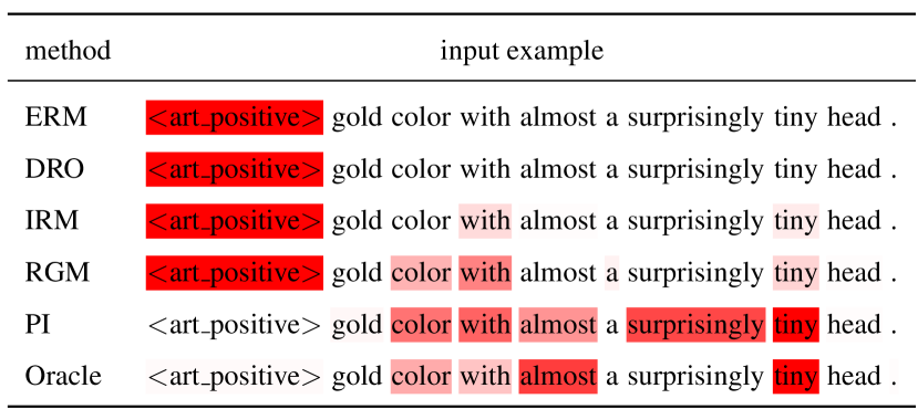
Figure 5: Visualizing word importance on Beer Look. Only PI and Oracle ignore the artificial token and correctly predict the input as negative. We will add more examples in the update.

What features does pi look at? To understand what features different methods rely on, we plot the word importance on Beer Look in Figure 5. For the given input example, we evaluate the prediction change as we mask out each input token. We observe that only PI and Oracle ignore the spurious feature and predict the label correctly. Comparing to ERM, IRM and RGM focus more on the causal feature such as ‘tiny’. However, they still heavily rely on the spurious feature.

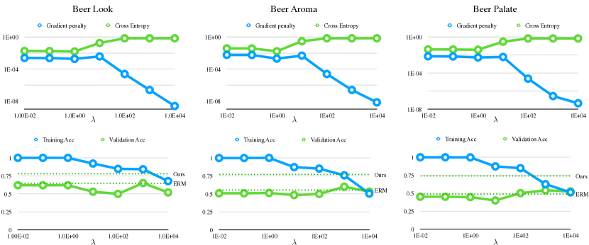
Figure 6: Performance of IRM as we adjust the weight of the gradient penalty. We observe that while the gradient penalty term is always orders of magnitude smaller than the cross entropy loss, the model is still able to overfit the unstable correlations in the training environments. As we further increase the penalty, the training & validation performance quickly drop to that of ERM.

	ERM		DRO		IRM		RGM		Ours
Accuracy	Worst	Avg	Worst	Avg	Worst	Avg	Worst	Avg	Worst	Avg
Adenocarcinoma	33.33	72.91	77.29	79.23	55.56	78.40	55.56	78.12	80.24	84.74
Polyp syndrom	44.44	74.63	77.29	78.79	55.56	76.31	66.67	78.73	69.23	81.28
Brain cancer	55.56	78.51	77.14	78.09	55.56	78.59	67.55	82.33	79.94	87.95
Breast cancer	66.49	80.47	75.00	78.84	66.87	80.56	64.38	79.81	80.32	83.12
Colorectal cancer	66.54	80.50	69.31	77.94	64.96	81.28	66.93	80.33	76.24	81.71
Endometrial cancer	66.98	80.60	76.19	80.21	66.03	82.60	66.98	81.77	80.32	83.26
Gastric cancer	62.96	79.94	76.95	81.65	62.96	80.03	59.26	78.87	79.44	85.92
Hepatobiliary cancer	44.44	73.01	60.00	73.89	55.56	77.19	55.56	76.22	60.00	78.94
Kidney cancer	16.67	66.66	50.00	68.70	33.33	73.07	33.33	71.31	50.00	74.76
Lung cancer	44.44	74.76	62.50	74.58	38.89	74.28	50.00	74.75	70.31	78.85
Melanoma	66.67	80.55	66.67	78.87	66.67	83.32	66.67	79.69	80.06	86.67
Neoplasia	50.00	75.98	33.33	69.10	33.33	71.97	50.00	75.18	70.00	80.06
Ovarian cancer	65.31	80.16	77.20	79.30	66.80	80.64	66.33	79.53	73.47	82.76
Pancreatic cancer	67.18	80.93	75.82	78.74	63.64	79.69	63.64	79.67	80.06	84.31
Prostate cancer	63.96	85.77	51.04	77.48	64.29	85.21	65.58	83.92	78.90	86.75
Rectal cancer	66.67	78.78	64.10	80.37	66.67	78.86	67.54	80.80	71.79	84.59
Thyroid cancer	50.00	77.18	75.00	83.06	66.86	84.05	67.73	82.56	80.23	87.85
Average	54.80	77.73	67.34	77.58	57.86	79.18	60.81	79.03	74.15	83.15

Table 7: Worst-group and average-group accuracy across 17 attributes on ASK2ME.

	ERM		DRO		IRM		RGM		Ours
	Worst	Avg	Worst	Avg	Worst	Avg	Worst	Avg	Worst	Avg
5_o_Clock_Shadow	53.33	81.51	90.00	92.05	80.00	85.93	66.67	87.22	83.33	89.65
Arched_Eyebrows	72.14	87.16	90.42	92.68	84.43	87.85	88.95	92.60	90.56	92.31
Attractive	67.21	85.84	90.77	92.22	82.57	87.28	86.64	91.94	89.98	91.86
Bags_Under_Eyes	72.46	86.16	90.59	92.04	81.34	86.84	88.52	92.13	89.12	92.12
Bald	75.98	91.23	91.73	93.04	71.39	82.21	91.50	94.81	91.68	93.42
Bangs	73.85	87.80	90.84	92.91	81.70	87.38	88.05	92.21	90.24	92.33
Big_Lips	73.46	87.14	90.59	92.55	84.16	87.87	89.54	92.65	90.52	92.17
Big_Nose	71.43	86.00	91.58	92.97	84.99	88.43	91.22	93.78	91.36	92.87
Black_Hair	75.98	90.91	89.62	93.77	78.63	89.16	90.66	94.02	88.10	93.30
Blurry	51.23	81.06	86.56	90.14	79.36	85.73	79.01	89.71	85.61	89.39
Brown_Hair	43.68	79.17	64.37	85.74	78.16	83.39	72.41	87.30	59.77	83.83
Bushy_Eyebrows	72.73	86.52	72.73	88.83	81.82	87.51	81.82	91.26	81.82	90.77
Chubby	9.52	70.69	61.90	84.63	76.19	82.91	47.62	82.32	71.43	86.59
Double_Chin	50.00	80.73	90.66	91.76	78.52	86.35	91.50	92.74	90.21	92.45
Eyeglasses	58.06	82.83	90.32	92.02	80.44	85.71	77.42	89.34	88.71	91.17
Goatee	0.00	68.26	0.00	70.08	84.80	90.83	91.50	95.66	91.63	94.59
Gray_Hair	60.71	82.53	69.08	87.73	42.60	76.20	85.71	89.56	68.26	88.18
Heavy_Makeup	66.06	85.68	89.69	92.22	84.18	87.20	84.43	91.49	90.01	91.86
High_Cheekbones	73.33	86.62	90.78	92.21	84.42	87.13	89.02	92.27	90.39	91.72
Gender.	46.67	80.14	85.56	90.87	74.44	83.93	70.00	87.73	90.56	91.52
Mouth_Slightly_Open	74.22	87.01	91.27	92.33	84.51	87.42	91.01	92.56	91.74	91.85
Mustache	50.00	80.89	91.72	95.38	50.00	78.58	91.50	95.97	91.60	94.93
Narrow_Eyes	69.23	85.54	90.05	91.85	82.94	87.00	88.46	91.84	91.69	91.90
No_Beard	39.39	78.10	84.85	90.97	72.73	83.80	57.58	85.00	84.85	90.43
Oval_Face	75.16	87.20	90.71	92.40	84.22	87.70	91.24	92.76	90.31	91.90
Pale_Skin	75.44	87.99	90.30	91.54	81.67	85.97	91.37	92.46	89.55	92.02
Pointy_Nose	73.34	87.18	91.19	92.42	84.87	87.69	89.29	92.55	91.07	92.00
Receding_Hairline	66.67	84.75	90.98	91.86	80.56	84.34	83.33	91.11	87.96	90.97
Rosy_Cheeks	74.90	88.17	91.40	93.32	84.88	88.59	90.55	93.00	91.49	92.71
Sideburns	38.46	77.84	84.62	90.69	76.92	84.14	76.92	89.72	91.35	93.75
Smiling	75.91	86.87	91.59	92.31	84.14	87.29	91.10	92.49	91.53	91.88
Straight_Hair	74.00	86.60	90.27	92.05	84.37	87.41	88.36	92.37	91.55	91.92
Wavy_Hair	74.22	86.88	91.41	92.40	84.15	87.41	88.81	92.21	91.64	91.88
Wearing_Earrings	75.36	86.77	91.67	92.63	84.78	87.70	90.88	92.55	91.51	92.19
Wearing_Hat	7.69	70.39	46.15	82.28	46.15	77.34	61.54	86.26	53.85	84.56
Wearing_Lipstick	59.37	83.61	89.47	91.88	82.53	86.01	79.37	90.10	90.32	91.57
Wearing_Necklace	74.57	87.26	91.09	92.47	82.26	87.42	89.53	92.17	90.73	92.21
Wearing_Necktie	25.00	74.52	90.00	91.56	80.00	84.31	35.00	79.32	91.44	92.53
Young	71.60	86.07	89.13	91.64	76.21	85.96	90.19	92.03	87.23	91.51
Average	60.06	83.63	84.25	90.83	78.51	85.79	82.52	90.95	87.04	91.41

Table 8: Worst-group and average-group accuracy for hair color prediction on CelebA.

References

- Ahuja et al. (2020) Ahuja, K., Shanmugam, K., Varshney, K., and Dhurandhar, A. Invariant risk minimization games. In International Conference on Machine Learning, pp. 145–155. PMLR, 2020.
- Arjovsky et al. (2019) Arjovsky, M., Bottou, L., Gulrajani, I., and Lopez-Paz, D. Invariant risk minimization. arXiv preprint arXiv:1907.02893, 2019.
- Bao et al. (2018) Bao, Y., Chang, S., Yu, M., and Barzilay, R. Deriving machine attention from human rationales. In Proceedings of the 2018 Conference on Empirical Methods in Natural Language Processing, pp. 1903–1913, 2018.
- Bao et al. (2019) Bao, Y., Deng, Z., Wang, Y., Kim, H., Armengol, V. D., Acevedo, F., Ouardaoui, N., Wang, C., Parmigiani, G., Barzilay, R., Braun, D., and Hughes, K. S. Using machine learning and natural language processing to review and classify the medical literature on cancer susceptibility genes. JCO Clinical Cancer Informatics, (3):1–9, 2019. doi: 10.1200/CCI.19.00042. URL https://doi.org/10.1200/CCI.19.00042. PMID: 31545655.
- Belinkov et al. (2019) Belinkov, Y., Poliak, A., Shieber, S. M., Van Durme, B., and Rush, A. M. Don’t take the premise for granted: Mitigating artifacts in natural language inference. In Proceedings of the 57th Annual Meeting of the Association for Computational Linguistics, pp. 877–891, 2019.
- Ben-Tal et al. (2013) Ben-Tal, A., Den Hertog, D., De Waegenaere, A., Melenberg, B., and Rennen, G. Robust solutions of optimization problems affected by uncertain probabilities. Management Science, 59(2):341–357, 2013.
- Bowman et al. (2015) Bowman, S. R., Angeli, G., Potts, C., and Manning, C. D. A large annotated corpus for learning natural language inference. In Proceedings of the 2015 Conference on Empirical Methods in Natural Language Processing, pp. 632–642, Lisbon, Portugal, September 2015. Association for Computational Linguistics. doi: 10.18653/v1/D15-1075. URL https://www.aclweb.org/anthology/D15-1075.
- Buolamwini & Gebru (2018) Buolamwini, J. and Gebru, T. Gender shades: Intersectional accuracy disparities in commercial gender classification. In Conference on fairness, accountability and transparency, pp. 77–91, 2018.
- Chang et al. (2020) Chang, S., Zhang, Y., Yu, M., and Jaakkola, T. S. Invariant rationalization. arXiv preprint arXiv:2003.09772, 2020.
- Choe et al. (2020) Choe, Y. J., Ham, J., and Park, K. An empirical study of invariant risk minimization. arXiv preprint arXiv:2004.05007, 2020.
- Clark et al. (2019) Clark, C., Yatskar, M., and Zettlemoyer, L. Don’t take the easy way out: Ensemble based methods for avoiding known dataset biases. In Proceedings of the 2019 Conference on Empirical Methods in Natural Language Processing and the 9th International Joint Conference on Natural Language Processing (EMNLP-IJCNLP), pp. 4060–4073, 2019.
- Deng et al. (2019) Deng, Z., Yin, K., Bao, Y., Armengol, V. D., Wang, C., Tiwari, A., Barzilay, R., Parmigiani, G., Braun, D., and Hughes, K. S. Validation of a semiautomated natural language processing–based procedure for meta-analysis of cancer susceptibility gene penetrance. JCO clinical cancer informatics, 3:1–9, 2019.
- Duchi & Namkoong (2018) Duchi, J. and Namkoong, H. Learning models with uniform performance via distributionally robust optimization. arXiv preprint arXiv:1810.08750, 2018.
- Gulrajani & Lopez-Paz (2020) Gulrajani, I. and Lopez-Paz, D. In search of lost domain generalization. arXiv preprint arXiv:2007.01434, 2020.
- He et al. (2019) He, H., Zha, S., and Wang, H. Unlearn dataset bias in natural language inference by fitting the residual. EMNLP-IJCNLP 2019, pp. 132, 2019.
- Hinton (2002) Hinton, G. E. Training products of experts by minimizing contrastive divergence. Neural computation, 14(8):1771–1800, 2002.
- Hu et al. (2018) Hu, W., Niu, G., Sato, I., and Sugiyama, M. Does distributionally robust supervised learning give robust classifiers? In International Conference on Machine Learning, pp. 2029–2037. PMLR, 2018.
- Jin et al. (2020) Jin, W., Barzilay, R., and Jaakkola, T. Enforcing predictive invariance across structured biomedical domains, 2020.
- Kim (2014) Kim, Y. Convolutional neural networks for sentence classification. In Proceedings of the 2014 Conference on Empirical Methods in Natural Language Processing (EMNLP), pp. 1746–1751, Doha, Qatar, October 2014. Association for Computational Linguistics. doi: 10.3115/v1/D14-1181. URL https://www.aclweb.org/anthology/D14-1181.
- Kingma & Ba (2014) Kingma, D. P. and Ba, J. Adam: A method for stochastic optimization. arXiv preprint arXiv:1412.6980, 2014.
- Krueger et al. (2020) Krueger, D., Caballero, E., Jacobsen, J.-H., Zhang, A., Binas, J., Zhang, D., Priol, R. L., and Courville, A. Out-of-distribution generalization via risk extrapolation (rex), 2020.
- LeCun et al. (1998) LeCun, Y., Bottou, L., Bengio, Y., and Haffner, P. Gradient-based learning applied to document recognition. Proceedings of the IEEE, 86(11):2278–2324, 1998.
- Lei et al. (2016) Lei, T., Barzilay, R., and Jaakkola, T. Rationalizing neural predictions. In Proceedings of the 2016 Conference on Empirical Methods in Natural Language Processing, pp. 107–117, 2016.
- Liu et al. (2015a) Liu, Z., Luo, P., Wang, X., and Tang, X. Deep learning face attributes in the wild. In Proceedings of the IEEE international conference on computer vision, pp. 3730–3738, 2015a.
- Liu et al. (2015b) Liu, Z., Luo, P., Wang, X., and Tang, X. Deep learning face attributes in the wild. In Proceedings of International Conference on Computer Vision (ICCV), December 2015b.
- Mahabadi et al. (2020) Mahabadi, R. K., Belinkov, Y., and Henderson, J. End-to-end bias mitigation by modelling biases in corpora. ACL, 2020.
- Mayr et al. (2018) Mayr, A., Klambauer, G., Unterthiner, T., Steijaert, M., Wegner, J. K., Ceulemans, H., Clevert, D.-A., and Hochreiter, S. Large-scale comparison of machine learning methods for drug target prediction on chembl. Chemical science, 9(24):5441–5451, 2018.
- McAuley et al. (2012) McAuley, J., Leskovec, J., and Jurafsky, D. Learning attitudes and attributes from multi-aspect reviews. In 2012 IEEE 12th International Conference on Data Mining, pp. 1020–1025. IEEE, 2012.
- McCoy et al. (2019) McCoy, T., Pavlick, E., and Linzen, T. Right for the wrong reasons: Diagnosing syntactic heuristics in natural language inference. In Proceedings of the 57th Annual Meeting of the Association for Computational Linguistics, pp. 3428–3448, Florence, Italy, July 2019. Association for Computational Linguistics. doi: 10.18653/v1/P19-1334. URL https://www.aclweb.org/anthology/P19-1334.
- Mikolov et al. (2018) Mikolov, T., Grave, E., Bojanowski, P., Puhrsch, C., and Joulin, A. Advances in pre-training distributed word representations. In Proceedings of the International Conference on Language Resources and Evaluation (LREC 2018), 2018.
- Oren et al. (2019) Oren, Y., Sagawa, S., Hashimoto, T., and Liang, P. Distributionally robust language modeling. In Proceedings of the 2019 Conference on Empirical Methods in Natural Language Processing and the 9th International Joint Conference on Natural Language Processing (EMNLP-IJCNLP), pp. 4218–4228, 2019.
- Peters et al. (2015) Peters, J., Bühlmann, P., and Meinshausen, N. Causal inference using invariant prediction: identification and confidence intervals. arXiv preprint arXiv:1501.01332, 2015.
- Peters et al. (2016) Peters, J., Bühlmann, P., and Meinshausen, N. Causal inference by using invariant prediction: identification and confidence intervals. Journal of the Royal Statistical Society. Series B (Statistical Methodology), pp. 947–1012, 2016.
- Sagawa et al. (2019) Sagawa, S., Koh, P. W., Hashimoto, T. B., and Liang, P. Distributionally robust neural networks for group shifts: On the importance of regularization for worst-case generalization. arXiv preprint arXiv:1911.08731, 2019.
- Sagawa* et al. (2020) Sagawa*, S., Koh*, P. W., Hashimoto, T. B., and Liang, P. Distributionally robust neural networks. In International Conference on Learning Representations, 2020. URL https://openreview.net/forum?id=ryxGuJrFvS.
- Sagawa et al. (2020) Sagawa, S., Raghunathan, A., Koh, P. W., and Liang, P. An investigation of why overparameterization exacerbates spurious correlations. In International Conference on Machine Learning (ICML), 2020.
- Sakaguchi et al. (2020) Sakaguchi, K., Le Bras, R., Bhagavatula, C., and Choi, Y. Winogrande: An adversarial winograd schema challenge at scale. In Proceedings of the AAAI Conference on Artificial Intelligence, volume 34, pp. 8732–8740, 2020.
- Sanh et al. (2021) Sanh, V., Wolf, T., Belinkov, Y., and Rush, A. M. Learning from others’ mistakes: Avoiding dataset biases without modeling them. In International Conference on Learning Representations, 2021. URL https://openreview.net/forum?id=Hf3qXoiNkR.
- Schuster et al. (2019) Schuster, T., Shah, D., Yeo, Y. J. S., Roberto Filizzola Ortiz, D., Santus, E., and Barzilay, R. Towards debiasing fact verification models. In Proceedings of the 2019 Conference on Empirical Methods in Natural Language Processing and the 9th International Joint Conference on Natural Language Processing (EMNLP-IJCNLP), pp. 3410–3416, Hong Kong, China, November 2019. Association for Computational Linguistics. doi: 10.18653/v1/D19-1341. URL https://www.aclweb.org/anthology/D19-1341.
- Stacey et al. (2020) Stacey, J., Minervini, P., Dubossarsky, H., Riedel, S., and Rocktäschel, T. Avoiding the Hypothesis-Only Bias in Natural Language Inference via Ensemble Adversarial Training. In Proceedings of the 2020 Conference on Empirical Methods in Natural Language Processing (EMNLP), pp. 8281–8291, Online, November 2020. Association for Computational Linguistics. doi: 10.18653/v1/2020.emnlp-main.665. URL https://www.aclweb.org/anthology/2020.emnlp-main.665.
- Utama et al. (2020) Utama, P. A., Moosavi, N. S., and Gurevych, I. Towards debiasing nlu models from unknown biases. In Proceedings of the 2020 Conference on Empirical Methods in Natural Language Processing (EMNLP), pp. 7597–7610, 2020.
- Woodward (2005) Woodward, J. Making things happen: A theory of causal explanation. Oxford university press, 2005.
- Wu et al. (2018) Wu, Z., Ramsundar, B., Feinberg, E. N., Gomes, J., Geniesse, C., Pappu, A. S., Leswing, K., and Pande, V. Moleculenet: a benchmark for molecular machine learning. Chemical science, 9(2):513–530, 2018.
- Yang et al. (2019) Yang, K., Swanson, K., Jin, W., Coley, C., Eiden, P., Gao, H., Guzman-Perez, A., Hopper, T., Kelley, B., Mathea, M., et al. Analyzing learned molecular representations for property prediction. Journal of chemical information and modeling, 59(8):3370–3388, 2019.
- Zellers et al. (2019) Zellers, R., Holtzman, A., Bisk, Y., Farhadi, A., and Choi, Y. HellaSwag: Can a machine really finish your sentence? In Proceedings of the 57th Annual Meeting of the Association for Computational Linguistics, pp. 4791–4800, Florence, Italy, July 2019. Association for Computational Linguistics. doi: 10.18653/v1/P19-1472. URL https://www.aclweb.org/anthology/P19-1472.