Weighted monotonicity theorems and applications to minimal surfaces of $\mathbb{H}^{n}$ and $S^{n}$

Abstract.

We prove that in a Riemannian manifold $M$, each function whose Hessian is proportional the metric tensor yields a weighted monotonicity theorem. Such function appears in the Euclidean space, the round sphere ${S}^{n}$ and the hyperbolic space $\mathbb{H}^{n}$ as the distance function, the Euclidean coordinates of $\mathbb{R}^{n+1}$ and the Minkowskian coordinates of $\mathbb{R}^{n,1}$. Then we show that weighted monotonicity theorems can be compared and that in the hyperbolic case, this comparison implies three $SO(n,1)$-distinct unweighted monotonicity theorems. From these, we obtain upper bounds of the Graham–Witten renormalised area of a minimal surface in term of its ideal perimeter measured under different metrics of the conformal infinity. Other applications include a vanishing result for knot invariants coming from counting minimal surfaces of $\mathbb{H}^{n}$ and a quantification of how antipodal a minimal submanifold of $S^{n}$ has to be in term of its volume.

1. Introduction

The classical monotonicity theorem dictates how a minimal submanifold of the Euclidean space distributes its volume between spheres of different radii centred around the same point. In the present paper, we prove the following three monotonicity results for minimal submanifolds of the hyperbolic space. Let $\Sigma$ be a minimal $k$-submanifold, $O$ be an interior point of $\mathbb{H}^{n}$ and denote by $A(t)$ be the $k$-volume of $\Sigma_{t}=\Sigma\cap B_{\cosh t}(O)$, the region of $\Sigma$ of distance at most $\cosh t$ from $O$. Define the function $Q_{\delta}(a,t)$ with parameter $\delta=-1,0,$ or $+1$ as:

(1.1) $$Q_{\delta}(a,t):=\int_{a}^{t}(t^{2}+\delta)^{\frac{k}{2}-1}dt+\frac{1}{ka}(a^{2}+\delta)^{\frac{k}{2}}$$

Theorem 1.1 (Time-monotonicity).

Let $d$ be the hyperbolic distance from $O$ to $\Sigma$, $a$ be any number in the interval $[1,\cosh d]$. Then the function

$$\Phi_{a}(\Sigma,t)=\frac{A(t)}{Q_{-1}(a,t)}\quad\text{is increasing in }t.$$

When $a=1$, Theorem 1.1 was proved by Anderson [2, Theorem 1]. For any submanifold $\Sigma$, if $\cosh d\geq a_{1}\geq a_{2}$, then the monotonicity of $\Phi_{a_{1}}$ implies that of $\Phi_{a_{2}}$. It is therefore optimal to choose $a$ in Theorem 1.1 to be $a=\cosh d$. In the language of the Comparison Lemma 3.11, the monotonicity of $\Phi_{a_{2}}$ is weaker than that of $\Phi_{a_{1}}$.

There are 2 other versions of Theorem 1.1, in which the interior point $O$ is replaced by a totally geodesic hyperplane $H$ and a point $b$ on the sphere at infinity $S_{\infty}$. We assume that in the compatification of $\mathbb{H}^{n}$ as the unit ball, the closure of $\Sigma$ does not intersect $H$ or contain $b$. In a half-space model associated to $b$, this means that $\Sigma$ has a maximal height $x_{\max}<+\infty$.

Theorem 1.2 (Space-monotonicity).

Let $a$ be any number in $(0,\sinh d]$ and $A(t)$ be the volume of the region $\Sigma_{t}$ of $\Sigma$ that is of distance at most $\sinh t$ from $H$. Then the function

$$\frac{A(t)}{Q_{+1}(a,t)}\quad\text{is increasing in }t.$$

Theorem 1.3 (Null-monotonicity).

Let $a$ be any number in $(0,x_{\max}^{-1}]$ and $A(t)$ be the volume of the region $\Sigma_{t}$ of $\Sigma$ with height at least $\frac{1}{t}$ in a half space model associated to $b$. Then the function

$$\frac{A(t)}{Q_{0}(a,t)}\quad\text{is increasing in }t.$$

These theorems can be seen as statements about volume distribution of a minimal submanifold among level sets of the time, space and null coordinates of $\mathbb{H}^{n}$. These are pullbacks of the coordinate functions of $\mathbb{R}^{n,1}$ via the hyperboloid model. These theorems are obtained in two steps. First, we prove that for any function $h$ on a Riemannian manifold $(M,g)$ with

(1.2) $$\operatorname{Hess}h=Ug,\quad h\in C^{2}(M),U\in C^{0}(M)$$

there is a naturally weighted monotonicity theorem for minimal submanifolds of $M$. This is a statement about the weighted volume distribution of the submanifold among level sets of $h$. Here the volume is weighted by $U$ and the density is obtained by normalising this volume by that of a gradient tube of $h$ (see Definitions 3.3 and 3.4). The coordinate functions of $\mathbb{R}^{n,1}$ and $\mathbb{R}^{n}$ pull back to functions on $\mathbb{H}^{n}$ and $S^{n}$ that satisfy (1.2). In the second step, we prove a comparison lemma which, in the hyperbolic case, gives us the unweighted volume distribution which are Theorems 1.1, 1.2, 1.3. More generally, these theorems also hold for tube extensions of minimal submanifolds (cf. Definition 3.1).

Since (1.2) is local, more examples for (1.2) can be constructed as quotient of $M$ by a symmetry group preserving $h$. Fuchsian manifolds are obtained this way (cf. Example 2.5) and Theorem 1.2 also holds there, given that one replaces $H$ by the unique totally geodesic surface.

There are two major differences, if one is to apply the previous argument for the Euclidean coordinates of $S^{n}$. First, all coordinate functions of $S^{n}$ are the same up to isometry whilst a Minkowskian coordinate $\xi$ of $\mathbb{H}^{n}$ falls into one of the three types depending on the norm of $d\xi$ in $\mathbb{R}^{n,1}$. Secondly, for the Euclidean coordinates of $S^{n}$, the natural weight is weaker than the uniform weight. This means that we cannot recover, from the Comparison Lemma 3.11, the unweighted volume distribution of a minimal submanifold. In fact, the unweighted density of the Clifford torus of $S^{3}$ is not monotone, even in a hemisphere. Despite this, the framework developed here can be used to prove (cf. Proposition 4.6) that the further a minimal submanifold of $S^{n}$ is from being antipodal, the larger its volume has to be. Here we quantify antipodalness by:

Definition 1.4.

A subset $X$ of $S^{n}$ is $\epsilon$-antipodal if the antipodal point of any point in $X$ is at distance at most $\epsilon$ from $X$.

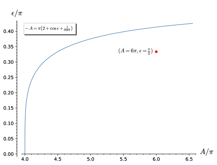
Figure 3. The function $\epsilon(A,2)$. The red point is the data for Veronese surface.

It is clear that 0-antipodal is antipodal and that any subset of $S^{n}$ is $\pi$-antipodal. The relation between $\epsilon$ and the volume $A$ of a minimal surface is drawn in Figure 3. Proposition 4.6 also confirms, in the non-embedded case, a conjecture by Yau on the second lowest volume of minimal hypersurfaces of $S^{n}$, cf. Remark 4.9.

Another application of the new monotonicity theorems is an isoperimetric inequality for complete minimal surfaces of $\mathbb{H}^{n}$. The area of these surfaces is necessarily infinite and can be renormalised according to Graham and Witten [12]. Let $A(\epsilon)$ be the area of the part of the surface that is $\epsilon$-far from the sphere at infinity $S_{\infty}$. They proved that it has the following expansion $A(\epsilon)=\frac{L}{\epsilon}+\mathcal{A}_{R}+O(\epsilon)$, where the coefficient $\mathcal{A}_{R}$, called the renormalised area, is an intrinsic quantity of the surface. We will give upper bounds of $\mathcal{A}_{R}$ by the length of the ideal boundary measured in different metrics in the conformal class at infinity. These metrics are obtained as the limit of $\xi^{-2}g_{\mathbb{H}}$ on $S_{\infty}$, which are finite almost everywhere. Depending on the type of $\xi$, they are either round metrics, flat metrics, or doubled hyperbolic metrics.

Theorem 1.5.

Let $\Sigma\subset\mathbb{H}^{n}$ be a minimal surface with ideal boundary $\gamma$ in $S_{\infty}$. Let $O$ be an interior point of $\mathbb{H}^{n}$ and $|\gamma|_{g_{O}}$ be the length of $\gamma$ measured in the round metric $g_{O}$ on $S_{\infty}$ associated to $O$. Then

(1.3) $$\mathcal{A}_{R}(\Sigma)+\frac{1}{2}\left(\cosh d+\frac{1}{\cosh d}\right)|\gamma|_{g_{O}}\leq 0$$

where $d$ is the distance from $O$ to $\Sigma$.

Theorem 1.5 relies on a simple remark (Lemma 3.9) about the extra information gained from a monotonicity theorem on the tube extension of a minimal submanifold. It implies in particular that the volume of a minimal submanifold of $\mathbb{H}^{n}$ is not larger than that of the tube competitor. The estimate (1.3) follows from substituting the volume bound given by Theorem 1.1 to the Graham–Witten expansion.

The volume bound corresponding to Anderson’s monotonicity (Theorem 1.1 with $a=1$) was obtained by Choe and Gulliver [8] by a different method. Plugging this into the Graham–Witten expansion, we have the following weaker version of (1.3):

(1.4) $$\mathcal{A}_{R}(\Sigma)+\sup_{\text{round }\tilde{g}}|\gamma|_{\tilde{g}}\leq 0$$

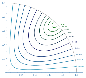
(a) in $\mathbb{H}^{4}$ with different values of $C$.

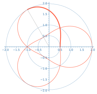
(b) in ${S}^{4}$ with $\theta_{C}\approx\frac{2\pi}{3}$. The unit circle represents the Clifford torus.

Figure 1. The profile curve of $M_{C}$

The estimate (1.4) was also independently proved by Jacob Bernstein [4]. To illustrate the extra factor in (1.3), we test it on a family of rotational minimal annuli $M_{C}$ in $\mathbb{H}^{4}$, indexed by a real number $C$. Here the rotation is given by changing the phase of the 2 complex variables of $\mathbb{C}^{2}\cong\mathbb{R}^{4}$ by an opposite number. The profile curves of these annuli are drawn in Figure 1(a). Their ideal boundary are pairs of round circles that form Hopf links in $S_{\infty}$. Whilst (1.4) only says $\mathcal{A}_{R}\leq-4\pi$, (1.3) shows that they tend to $-\infty$. Moreover, the perimeter term of (1.3) also captures the decreasing rate of $\mathcal{A}_{R}$. These two quantities are drawn in Figure 3. The graph was plotted in log scale, in which the two curves are asymptotically parallel. So the gap between them should be interpreted as a multiplicative factor between the two quantities, which is approximately 1.198.

Theorems 1.2 and 1.3 also give two other upper bounds of area, and thus two other isoperimetric inequalities:

Theorem 1.6.

Let $H$, $b$, $\Sigma$ be a totally geodesic plane, a boundary point, and a complete minimal surfaces satisfying the condition of Theorems 1.2 and 1.3. We denote by $|\gamma|_{H}$ and $|\gamma|_{b}$ the length of the boundary curve under the doubled hyperbolic metric and the flat metric associated to $H$ and $b$. Then

(1.5) $$\mathcal{A}_{R}(\Sigma)+\frac{1}{2}\left(\sinh d-\frac{1}{\sinh d}\right)|\gamma|_{H}\leq 0$$

(1.6) $$\mathcal{A}_{R}(\Sigma)+\frac{1}{2}\frac{|\gamma|_{b}}{x_{\max}}\leq 0$$

Here $d$ is the distance from $\Sigma$ to $H$ and $x_{\max}$ is the maximal height of $\Sigma$ in the half-space model where $b$ is at infinity.

It can be seen either directly from (1.3) or from (1.5) and a rescaling argument (cf. Figure 5) that $\mathcal{A}_{R}\leq-2\pi$ for any minimal surface. The estimate (1.6), on the other hand, seems to be optimised for a completely different type of surface than totally geodesic discs. For the discs, $\mathcal{A}_{R}=-2\pi$ whilst the perimeter term in (1.6) is $+\pi$ and one may hope to drop the constant $\frac{1}{2}$ there. However, the family of minimal annuli of $\mathbb{H}^{3}$ found by Mori [19] and whose renormalised area was computed by Krtouš and Zelnikov [16], show that the constant $\frac{1}{2}$ of (1.6) cannot be replaced by any number bigger than $0.59$.

Each $(k-1)$-submanifold $\gamma$ of $S_{\infty}$ induces a function $V_{\gamma}$ on $\mathbb{H}^{n}$, whose value at a point $O$ is the volume of $\gamma$ under the round metric $g_{O}$. The visual hull of $\gamma$ was defined by Gromov [13] as the set of points where $V_{\gamma}$ is at least the volume of the Euclidean $(k-1)$-sphere. Another application of Theorem 1.1 is:

Corollary 1.7.

A minimal submanifold of $\mathbb{H}^{n}$ is contained in the visual hull of its ideal boundary.

Proposition 1.8.

Let $L:=L_{1}\sqcup L_{2}$ be a separated union of two $(k-1)$-submanifold $L_{1},L_{2}$ of ${S}^{n-1}$. Then we can rearrange $L$ in its isotopy class such that there is no connected minimal $k$-submanifold $\Sigma$ of $\mathbb{H}^{n}$ whose ideal boundary is $L$.

Proof.

In the Poincaré ball model, we isotope $L$ so that $L_{1}$ (or $L_{2}$) is contained in a small ball centred at the North (respectively South) pole and so that the Euclidean volume of $L$ is less than $\frac{1}{2}\omega_{k-1}$. It suffices to prove that any minimal submanifold filling $L$ has no intersection with the equatorial hyperplane. By convexity, such intersection is contained in a small ball centred at the origin $O$. If it was non-empty, by a small Möbius transform we could suppose that $\Sigma$ contains $O$ while keeping the Euclidean length of $L$ less than $\omega_{k-1}$. This is a contradiction. ∎

The visual hull and the proof of Proposition 1.8 can be visualised in Figure 5.

The motivation for Proposition 1.8 comes from recent works of Alexakis, Mazzeo [1] and Fine [10]. The counting problem for minimal surfaces of $\mathbb{R}^{3}$ bounded by a given curve traces back to Tomi–Tromba’s resolution of the embedded Plateau problem [21] and was studied in a more general context by White [22]. In the hyperbolic space, one can ask the ideal boundary of the minimal surface to be an embedded curve $\gamma$ in the sphere at infinity. This problem was studied by Alexakis and Mazzeo in $\mathbb{H}^{3}$ and by Fine in $\mathbb{H}^{4}$. Denote by $\mathcal{C}$ the Banach manifold of curves in $S_{\infty}$, $\mathcal{S}$ the space of minimal surfaces and $\pi:\mathcal{S}\longrightarrow\mathcal{C}$ the map sending a surface to its ideal boundary. The counting problem consists of proving $\mathcal{S}$ is a Banach manifold and establishing a degree theory for $\pi$. The degree is constant in the isotopy class of $\gamma$ and defines a knot/link invariant. Proposition 1.8 shows that this invariant is multiplicative in $\gamma$: any minimal surface filling a separated union of links is union of surfaces filling each one individually.

It was proved, in the works mentioned above, that the map $\pi$ is Fredholm and of index 0. This is because the stability operator is self-adjoint and elliptic or 0-elliptic. The properness of $\pi$ is however more subtle. In $\mathbb{H}^{4}$, this can be seen via the family $M_{C}$: as $C$ decreases to $0$, their boundary converges to the standard Hopf link $\{zw=0\}\cap S^{3}$ and the waist of $M_{C}$ collapses. In fact, it can be proved (Proposition 4.10) that the only minimal surface of $\mathbb{H}^{4}$ filling the standard Hopf link is the pair of discs. One can still hope that properness holds on a residual subset of $\mathcal{C}$, as the previous phenomenon happens in codimension 2 of $\gamma$.

Since monotonicity theorems are inequalities, they still hold when the Hessian of the function $h$ is comparable to the metric as symmetric 2-tensors. We will see in Section 5 that such function arises naturally as the distance function in a Riemannian manifold whose sectional curvature is bounded from above. When the curvature is negative, this weighted monotonicity theorem also implies the unweighted version. In the case of positive curvature, an unweighted monotonicity inequality was obtained by Scharrer [20].

Acknowledgements.

The author thanks Joel Fine for introducing him to minimal surfaces and harmonic maps in hyperbolic space and for proposing the search of the minimal annuli in $\mathbb{H}^{4}$. He also wants to thank Christian Scharrer for the reference [14] and Benjamin Aslan for helpful discussions on [3] and [15]. The author was supported by Excellence of Science grant number 30950721, Symplectic techniques in differential geometry.

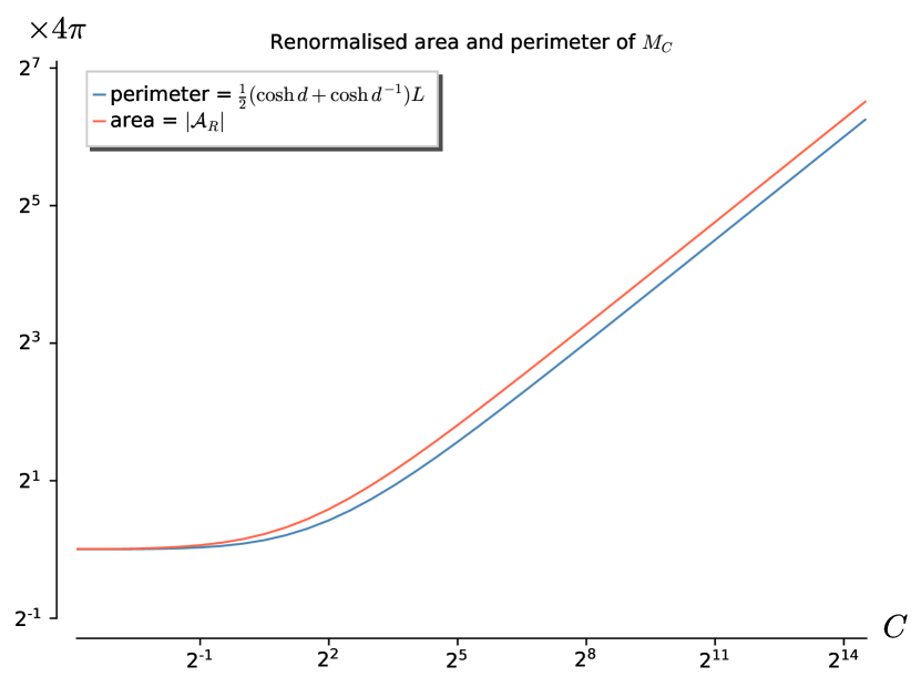
Figure 2. The area and perimeter terms of (1.3) for the annuli $M_{c}$ in $\mathbb{H}^{4}$.

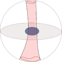
Figure 4. Any minimal surface $\Sigma$ filling the link $L$ (red) is contained in its visual hull (pink). It cannot intersect the blue region because of the visual hull. So $\Sigma$ has no intersection with the equatorial disc and has to be disconnected.

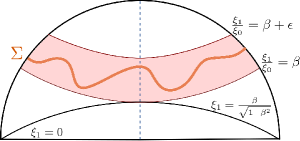
Figure 5. For a pair $(\xi_{0},\xi_{1})$ of time and space coordinates in the same Minkowskian system, the function $\frac{\xi_{1}}{\xi_{0}}$ foliates $\mathbb{H}^{n}$ into totally geodesic leaves. By a Mobius transform, $\Sigma$ can be put in the region $\beta\leq\frac{\xi_{1}}{\xi_{0}}\leq\beta+\epsilon$, which guarantees $\xi_{1}\geq\ \frac{\beta}{\sqrt{1-\beta^{2}}}$ on $\Sigma$. Plugging this into (1.5) and sending $\epsilon$ then $\beta$ to 0, one has $\mathcal{A}_{R}(\Sigma)\leq-2\pi$.

2. The hyperbolic space and the sphere as warped spaces.

A metric on a Riemannian manifold $M=N\times[a,b]$ is a warped product if it has the form

(2.1) $$g=dr^{2}+f^{2}(r)g_{N}$$

where $r\in[a,b]$ and $g_{N}$ is a Riemannian metric on $N$. It can be checked that an anti-derivative $h$ of the warping function $f$ satisfies $\operatorname{Hess}(h)=f^{\prime}(r)g$. On the other hand, if such function $h$ exists, the space can be written locally as a warped product by the level sets of $h$.

Proposition 2.1 (cf. [5]).

Let $h$ be a $C^{2}$ function on $(M,g)$ with no critical point. Suppose that the level sets of $h$ are connected and that

(2.2) $$\operatorname{Hess}h=U.g$$

for a function $U\in C^{0}(M)$. Then:

1. $U=U(h)$ is a function of $h$, i.e. a precomposition of $h$ by a function $U:\mathbb{R}\longrightarrow\mathbb{R}$. So is the function $V:=|dh|^{2}\in C^{1}(M)$ and we have $\frac{dV}{dh}=2U$.

2. The metrics $g_{a},g_{b}$ induced from $g$ on level sets $h^{-1}(a)$ and $h^{-1}(b)$ are related by $\frac{g_{a}}{V(a)}=\frac{g_{b}}{V(b)}$ via the inverse gradient flow of $h$. This defines a metric $\tilde{g}$ on level sets of $h$ under which the flow is isometric. The the metric $g$ pulls back, via the flow map $h^{-1}(a)\times{\mathrm{Range}}(h)\longrightarrow M$, to

   (2.3) $$g=\frac{V(h)}{V(a)}g_{a}+\frac{dh^{2}}{V(h)}=V(h)\tilde{g}+\frac{dh^{2}}{V(h)}$$

   which is a warped product after a change of variable $dr=\frac{dh}{V(h)^{1/2}}$.

Proof.

For any vector field $v$, one has

(2.4) $$v(V)=2g(\nabla_{v}\nabla h,\nabla h)=2\operatorname{Hess}(h)(v,\nabla h)=2Ug(v,\nabla h)$$

It follows, by choosing $v$ in (2.4) to be any vector field tangent to level sets of $h$, that $V$ is constant on the level sets of $h$. Then choose $v$ to be the inverse gradient $\frac{\nabla h}{|\nabla h|^{2}}$, we have $(\nabla h)V=2U|\nabla h|^{2}$, so $U$ is also a function of $h$ and $\frac{dV}{dh}=2U$.

For the second part, let $v_{t}$ be a vector field of $M$ tangent to level sets $h^{-1}(t)$ given by pushing forward via the flow of $u$ a vector field $v_{a}$ tangent to $h^{-1}(a)$. By definition of Lie bracket, $[v_{t},u]=0$ for all $t$, and so

$$\frac{d}{dt}|v_{t}|^{2}=2g(\nabla_{u}v_{t},v_{t})=2g(\nabla_{v_{t}}u,v_{t})=\frac{2}{|\nabla h|^{2}}\operatorname{Hess}(h)(v_{t},v_{t})=\frac{V^{\prime}}{V}|v_{t}|^{2}.$$

Here in the third equality, we used the fact that $v_{t}$ is orthogonal to the gradient of $h$. We conclude that $\frac{|v_{t}|^{2}}{V(t)}$ is constant along the flow and so $\frac{g_{a}}{V(a)}=\frac{g_{b}}{V(b)}$ for all $a,b$ in the range of $h$. ∎

The metric $\tilde{g}$ is the $g_{N}$ of (2.1) and the restrictions of $\tilde{g}$ and $g$ on the level sets of $h$ are conformal. We will also use $\tilde{g}$ to denote the metric $V(h)^{-1}g$ on $M$ and will call it the normalised metric.

In applications, we will only assume that the function $h$ satisfies (2.2) on $M$ and it is allowed to have critical points, as in the following examples.

Example 2.2.

In the Euclidean space, the only functions satisfying (2.2) are the coordinates $x_{i},i=1,\dots,n$ (and their linear combinations) and the square of distance $\rho:=\frac{1}{2}\sum_{i=1}^{n}x_{i}^{2}$.

Example 2.3.

In the unit sphere ${S}^{n}=\{(x_{1},\dots,x_{n+1})\in\mathbb{R}^{n+1}:\sum_{i=1}^{n+1}x_{i}^{2}=1\}$, the $x_{i}$ satisfy (2.2) with $U=-x_{i},V=1-x_{i}^{2}$. It is more intuitive to choose $h$ to be $1-x_{i}$, for which $U=1-h$ and $V=2h-h^{2}$.

Example 2.4.

In the hyperbolic space $\mathbb{H}^{n}=\{(\xi_{0},\dots,\xi_{n})\in\mathbb{R}^{n,1}:\xi_{0}^{2}-\sum_{i=1}^{n}\xi_{i}^{2}=1,\xi_{0}>0\}$, the Minkowskian coordinates $\xi_{\alpha}$ satisfies (2.2) with $U=\xi_{\alpha},V=\xi_{\alpha}^{2}+|d\xi_{\alpha}|^{2}$. Here $|d\xi_{\alpha}|^{2}=-1$ if $\alpha=0$ and +1 if $\alpha\geq 1$. All null (light-type) coordinates can be written, up to a Möbius transform as $\xi_{l}=\xi_{0}-\xi_{1}$. They satisfy (2.2) with $U=\xi_{l}$ and $V=\xi_{l}^{2}$.

Unlike $S^{n}$, $\mathbb{H}^{n}$ can be written as warped product in 3 $SO(n,1)$-distinct ways. Geometrically, each time coordinate is uniquely defined by an interior point of $\mathbb{H}^{n}$ where it is minimised. Each space coordinate is uniquely defined by a totally geodesic hyperplane where it vanishes together with a coorientation. Each point on $S_{\infty}$ defines a null coordinate uniquely up to a multiplicative factor. In the the half space model with height coordinate $x>0$, such functions are given by $\frac{\lambda}{x},\lambda>0$.

The normalised metrics $\tilde{g}$ of $(\mathbb{R}^{n},\rho),({S}^{n},x_{i})$ and $(\mathbb{H}^{n},\xi_{0})$ are all round metrics on ${S}^{n-1}$. For a null coordinate associated to a point $b\in S_{\infty}$, $\tilde{g}$ is the flat metric on $S_{\infty}\setminus\{b\}$. For the space coordinate associated to a hyperplane $H$, $\tilde{g}$ is obtained by putting hyperbolic metrics on each component of $S_{\infty}\setminus\overline{H}$. We will call this a doubled hyperbolic metric. In all cases, $\tilde{g}$ lies in the conformal class at infinity.

Example 2.5.

Equation (2.2) is local and so will descend to the quotient whenever there is an isometric group action that preserves $h$. The subgroup of $SO_{+}(n,1)$ that preserves a space coordinate $\xi$ of $\mathbb{H}^{n}$ is $SO_{+}(n-1,1)$. When $n=3$, the quotient of $\mathbb{H}^{3}$ by a discrete subgroup of $SO_{+}(2,1)$ is called a Fuchsian manifold and the metric descends to a warped product:

$$g=dr^{2}+\cosh^{2}r.g_{\Sigma}\quad\text{on }\Sigma\times\mathbb{R},\qquad\xi=\sinh r$$

Here $\Sigma$ is a Riemann surface of genus at least $2$, equipped with the hyperbolic metric $g_{\Sigma}$.

3. Monotonicity Theorems and Comparison Lemma

Given a function $h$ on a Riemannian manifold $M$ and a submanifold $\Sigma$, we write $\int_{\Sigma,h\leq t}$ and $\int_{\Sigma,h=t}$ for the integration over the sub-level $h^{-1}(-\infty,t]$ and the level set $h=t$ of $h$ on $\Sigma$. The gradient vector of $h$ in $M$ is denoted by $\nabla h$ and its projection to the tangent of $\Sigma$ by $\nabla^{\Sigma}h$. We will write $\Delta_{\Sigma}h=\mathop{\rm div}\nolimits_{\Sigma}\nabla^{\Sigma}h$ for the rough Laplacian of $h$ on $\Sigma$. The volume of the $k$-dimensional unit sphere will be denoted by $\omega_{k}$. We will fix a function $h$ on $M$ that satisfies property (2.2).

Definition 3.1.

Let $\gamma$ be a $(k-1)$-submanifold of $M$. The forward $h$-tube $T_{\gamma}^{+}$ (respectively backward $h$-tube $T_{\gamma}^{-}$) built upon $\gamma$ is the $k$-submanifold obtained by flowing $\gamma$ along the gradient of $h$ forwards (respectively backwards) in time. We will denote their union by $T_{\gamma}$ and the intersection of $T_{\gamma}$ with the region $t_{1}\leq h\leq t_{2}$ by $T_{\gamma}(t_{1},t_{2})$.

The tube extension of a submanifold is its union with the forward tube built upon its boundary, as shown in Figure 6.

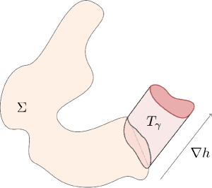
Figure 6. Extension of a submanifold by gradient tube of $h$.

Let $\gamma$ be a $(k-1)$-submanifold of a non-critical level set of $h=$, and $\mathcal{D}$ be a distribution of $k$-dimensional planes of $M$ along $\gamma$.

Definition 3.2.

The $\mathcal{D}$-parallel volume of $\gamma$ is

$$\left|\gamma^{\mathcal{D}}\right|:=\int_{\gamma}\cos\angle(\nabla h,\mathcal{D})\mathop{\rm vol}\nolimits^{k-1}_{\tilde{g}},$$

where the integral was taken with the volume form of the normalised metric $\tilde{g}$ and $\angle(\nabla h,\mathcal{D})$ is the angle between $\nabla h$ and $\mathcal{D}$. When $\nabla h$ is contained in $\mathcal{D}$ at every point of $\gamma$, $|\gamma^{\mathcal{D}}|$ is the $\tilde{g}$-volume of $\gamma$.

We will suppose that $\Sigma$ is a $k$-submanifold in the region $h\geq h_{0}$ of $M$ and that the intersection of $\Sigma$ and the level set $h=h_{0}$ has zero $k$-volume. This happens for example when the intersection is empty or a transversally cut out $(k-1)$-submanifold $\gamma_{0}$.

Definition 3.3.

A weight is a pair $(P,c)$ of a function $P:\mathbb{R}\longrightarrow\mathbb{R}$ and a real number $c$. We define the $(h_{0},(P,c))$-volume of $\Sigma$ by

(3.1) $$A_{h_{0},(P,c)}(\Sigma)(t):=\int_{\Sigma,h_{0}\leq h\leq t}P(h)+\frac{c}{k}|\gamma_{0}^{T\Sigma}|\ V(h_{0})^{k/2}$$

Most of the time, we fix the starting level $h_{0}$ and change the weight and so will often drop $h_{0}$ in the notation. When $h_{0}$ is chosen to be a critical value of $h$, the RHS of (3.1) no longer depends on $c$ and we drop it in the data of a weight.

Because the metric $g$ has the form (2.3), the $(P,c)$-volume of a tube $T_{\gamma}(h_{0},t)$, as a function of $t$, is independent of the choice of $\gamma$ up to a multiplicative factor:

(3.2) $$A_{(P,c)}(T_{\gamma}(h_{0},t))=\frac{|\gamma|_{\tilde{g}}}{\omega_{k-1}}Q_{(P,c)}(t),\qquad Q_{(P,c)}(t):=\omega_{k-1}\left[\int_{h_{0}}^{t}P(h)V^{\frac{k}{2}-1}(h)dh+\frac{c}{k}V(h_{0})^{\frac{k}{2}}\right]$$

Definition 3.4.

The $(P,c)$-density of $\Sigma$ is obtained by normalising its weighted volume by that of a tube:

(3.3) $$\Theta_{(P,c)}(t):=\frac{A_{(P,c)}(\Sigma)(t)}{Q_{(P,c)}(t)}.$$

Clearly, the density of a tube is constant in $t$. In (3.2), we choose to put the constant $\omega_{k-1}$ in $Q$ to be consistent with the classical monotonicity theorem ($h=\rho$ in Example 2.2). In the classical case with $h_{0}=0$, $h$-tubes are visually cones or discs.

We call the pair $(U,1)$ the natural weight. The naturally weighted volume of tubes simplifies to $Q_{(U,1)}(t)=\frac{\omega_{k-1}}{k}|\gamma|_{\tilde{g}}V^{k/2}(t)$, which is independent of the starting level $h_{0}$.

Theorem 3.5 (Naturally weighted monotonicity).

Let $h$ be a $C^{2}$ function on a Riemannian manifold $M$ that satisfies (2.2) with $U$ and $V=|\nabla h|^{2}$ being functions of $h$ such that $U=\frac{1}{2}V^{\prime}$. Let $\Sigma$ be a minimal $k$-submanifold in $M$. Then the naturally weighted density $\Theta_{(U,1)}(\Sigma)(t)$ is increasing in region $U>0$ and decreasing in region $U<0$.

Moreover, the conclusion also holds for the tube extension of minimal submanifolds.

Proof.

The Laplacian of $h$ on $\Sigma$ can be computed to be

$$\Delta_{\Sigma}h=kU.$$

This can be seen via the formula:

Lemma 3.6 (Leibniz rule).

Let $f:(\Sigma,g_{\Sigma})\longrightarrow(M,g)$ be a map between Riemannian manifolds and $\tau(f)$ be its tension field. Then for any $C^{2}$ function $h$ on $M$:

(3.4) $$\Delta_{\Sigma}(h\circ f)=\mathop{\rm Tr}\nolimits_{\Sigma}f^{*}\operatorname{Hess}h+dh.\tau(f)$$

In particular,

$$\Delta_{\Sigma}h=\mathop{\rm Tr}\nolimits_{\Sigma}\operatorname{Hess}h$$

if $\Sigma$ is either minimal or tangent to the gradient of $h$.

Because the volume forms of $g$ and $\tilde{g}$ on $\gamma$ are related by $\mathop{\rm vol}\nolimits_{g}^{k-1}=V^{\frac{k-1}{2}}\mathop{\rm vol}\nolimits_{\tilde{g}}^{k-1}$ and $\cos\angle(\nabla h,T\Sigma).V^{1/2}=|\nabla^{\Sigma}h|$, the second term in the definition of weighted volume (3.1) is $\frac{c}{k}\int_{\gamma_{0}}|\nabla^{\Sigma}h|$. By Stokes’ theorem,

(3.5) $$kA_{(U,1)}(\Sigma)(t)=\int_{\Sigma,h_{0}\leq h\leq t}\Delta_{\Sigma}h+\int_{\gamma_{0}}|\nabla^{\Sigma}h|=\int_{\Sigma,h=t}(\nabla^{\Sigma}h)\cdot n=\int_{\Sigma,h=t}|\nabla^{\Sigma}h|.$$

The last equality is because the outer normal of the sublevel set $h\leq t$ in $\Sigma$ is $n=\frac{\nabla^{\Sigma}h}{|\nabla^{\Sigma}h|}$. By the coarea formula,

$$\frac{dA_{(U,1)}(t)}{dt}=U(t)\int_{\Sigma,h=t}\frac{1}{|\nabla^{\Sigma}h|}.$$

Combining this with (3.5) and $|\nabla^{\Sigma}h|^{2}\leq V(h)$, one has $\frac{1}{U}\frac{dA_{h}}{dt}\geq\frac{kA_{h}}{V}$, or

$$\frac{1}{U}\frac{d}{dt}\left(\Theta_{(U,1)}(\Sigma)\right)\geq 0.$$

For the extension $\tilde{\Sigma}$ of $\Sigma$ by a forward tube built upon $\gamma=\partial\Sigma$, it suffices to rewrite (3.5) as

$$kA_{(U,1)}(\tilde{\Sigma})(t) =\left(\int_{\Sigma,h\leq t}+\int_{T^{+}_{\gamma},h\leq t}\right)\Delta h$$

$$=\int_{\Sigma,h=t}|\nabla^{\Sigma}h|+\int_{\gamma\cap\{h\leq t\}}|\nabla^{\Sigma}h|+\int_{T^{+}_{\gamma},h=t}|\nabla h|-\int_{\gamma\cap\{h\leq t\}}|\nabla h|$$

$$\leq\int_{\Sigma,h=t}|\nabla^{\Sigma}h|+\int_{T_{\gamma},h=t}|\nabla h|=\int_{\tilde{\Sigma},h=t}|\nabla^{\tilde{\Sigma}}h|.$$

∎

Remark 3.7.

We only need the ”$\leq$” sign in (3.5) and hence it suffices that $\Delta_{\Sigma}h\geq kU(h)$. Theorem 3.5 also holds if $\operatorname{Hess}h\geq U.g$, provided that $U$ and $V=|dh|^{2}$ are functions of $h$ with $U=\frac{1}{2}V^{\prime}$ (see Section 5).

The classical monotonicity theorem is recovered by applying Theorem 3.5 to the function $\rho$ of Example 2.2. On the other hand, Choe and Gulliver [7, Theorem 3] discovered that there are monotonicity theorems in $S^{n}$ and $\mathbb{H}^{n}$ if one weights the volume functional by the cosine (respectively hyperbolic cosine) of the distance function. These theorems come from applying Theorem 3.5 to Euclidean coordinates of Example 2.3 and time coordinates of Example 2.4.

Since the proof of Theorem 3.5 only uses integration by part, it can be adapted to stationary rectifiable $k$-currents or $k$-varifolds. Instead of integrating the Laplacian of $h$, it suffices to apply the first variation formula to a test vector field that is a suitable cut-off of the gradient of $h$. See [2, Theorem 1] and [9, $\S$7]

Theorem 3.5 can also be adapted for harmonic maps. Given a map $f:\Sigma\longrightarrow M$, we define its dimension at a point $p\in\Sigma$ to be the ratio $\frac{|df_{p}|^{2}}{|df_{p}|_{o}^{2}}$ of the tensor norm of the derivative at $p$ (also called energy density) and its operator norm, or $+\infty$ if the latter vanishes. Note that when $df_{p}$ is conformal, this is the dimension of $\Sigma$. The dimension of $f$, defined as the smallest dimension at all points, plays the role of $k$ in the argument.

The naturally weighted Dirichlet energy and naturally weighted density of $f$ are defined as

$$E_{(U,1)}(t):=\int_{\Sigma,h_{0}\leq h\circ f\leq t}U|df|^{2}+\int_{\Sigma,h\circ f=h_{0}}|d(h\circ f)|,\quad\Theta_{(U,1)}(t):=\frac{E_{(U,1)}(t)}{V(t)^{k/2}}.$$

Theorem 3.8.

Let $h,U,V$ be as in Theorem 3.5 and $f:\Sigma\longrightarrow M$ be a harmonic map. Then $\frac{d}{dt}\Theta_{h}$ has the same sign as $U$.

Proof.

By Lemma 3.6, $\Delta(h\circ f)=U|df|^{2}$ and by integration by part, $E_{(U,1)}(t)=\int_{\Sigma,h\circ f=t}|d(h\circ f)|$. One then compares $E_{(U,1)}$ with its derivative obtained from the coarea formula $\frac{d}{dt}E_{(U,1)}=U(t)\int_{\Sigma,h\circ f=t}\frac{|df|^{2}}{|d(h\circ f)|}$. The definition of $k$ guarantees $\frac{|df|^{2}}{|d(h\circ f)|}\geq k\frac{|d(h\circ f)|}{|dh|^{2}}$ and therefore

$$U^{-1}\frac{d}{dt}E_{(U,1)}(t)\geq\frac{k}{V}E_{(U,1)},$$

which is equivalent to $\frac{1}{U}\frac{d}{dt}\Theta_{h}\geq 0$. ∎

We will give another characterisation of the monotonicity in the extended region. For this, we suppose that $\Sigma$ is contained in the region $h_{0}\leq h\leq h_{1}$ as in Figure 7, with boundary composing of 2 parts: one (possibly empty) in level $h=h_{0}$ and one, called $\gamma$, in $h=h_{1}$. Let $\tilde{\Sigma}$ be the forward tube extension of $\Sigma$ built upon $\gamma$. Clearly the monotonicity of $\tilde{\Sigma}$ and $\Sigma$, under any weight, are the same in the region $[h_{0},h_{1}]$. In the region $h\geq h_{1}$, the monotonicity of $\tilde{\Sigma}$ is equivalent to a volume comparison between $\Sigma$ and the tube.

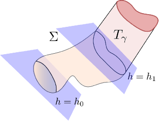
Figure 7. Illustration of Lemma 3.9.

Lemma 3.9.

Let $t_{1}<t_{2}$ be two numbers in $[h_{1},+\infty)$, then the following statements are equivalent:

1. $\Theta_{(P,c)}(\tilde{\Sigma})(t_{1})\leq\Theta_{(P,c)}(\tilde{\Sigma})(t_{2})$

2. $A_{(P,c)}(\Sigma)(h_{1})\leq A_{(P,c)}(T_{\gamma}(h_{0},h_{1}))$

Proof.

It follows from straightforward volume addition and the fact that the density of a tube is constant. ∎

By Theorem 3.5, we are mostly interested in the region of $M$ where $U$ is signed. By switching the sign of $h$, we can assume that $U\geq 0$. When one applies Lemma 3.9 to minimal submanifold, the assumption that $\Sigma$ belongs to the region $h_{0}\leq h\leq h_{1}$ becomes automatic. This is because $h\leq h_{1}$ on $\partial\Sigma$ and its restriction to $\Sigma$ is superharmonic $\Delta h=kU\geq 0$. Also, there is no critical point of $h$ in the region $U>0$ because the function $V(h)=|dh|^{2}$ satisfies $V^{\prime}=2U>0$.

Let $(P_{1},c_{1}),(P_{2},c_{2})$ be 2 positive weights, that is $P_{i}\geq 0$. The tube volumes, defined in (3.2), will be denoted by $Q_{1}(t),Q_{2}(t)$.

Definition 3.10.

We say that $(P_{1},c_{1})$ is weaker than $(P_{2},c_{2})$ and write $(P_{1},c_{1})\ll(P_{2},c_{2})$ if $\frac{P_{1}}{Q_{1}}\leq\frac{P_{2}}{Q_{2}}$ for all $t$, Equivalently, this means if $\frac{d}{dt}\frac{Q_{1}}{Q_{2}}\leq 0$, i.e. the $(P_{2},c_{2})$-volume of a $k$-dimensional tube increases faster than its $(P_{1},c_{1})$-volume.

Lemma 3.11 (Comparison).

Let $\Sigma\subset M^{n}$ be a $k$-submanifold not necessarily minimal and $(P_{1},c_{1}),(P_{2},c_{2})$ be two positive weights. Let $\Theta_{1},\Theta_{2}$ be the corresponding densities.

1. Suppose that $(P_{1},c_{1})\ll(P_{2},c_{2})$ and that $\Theta_{2}(\Sigma)$ is increasing. Then $\Theta_{1}$ is also increasing and we have $\Theta_{1}\leq\Theta_{2}$.

2. On the other hand, if $(P_{2},c_{2})\ll(P_{1},c_{1})$ and $\Theta_{2}(\Sigma)$ is increasing. Then we still have $\Theta_{1}\geq\Theta_{2}$.

Proof.

One has $P_{1}^{-1}\frac{dA_{(P_{1},c_{1})}}{dt}=P_{2}^{-1}\frac{dA_{(P_{2},c_{2})}}{dt}$ from coarea formula. Therefore

(3.6) $$\frac{Q_{1}}{P_{1}}\frac{d\Theta_{1}}{dt}+\omega_{k-1}V^{\frac{k}{2}-1}\Theta_{1}=\frac{Q_{2}}{P_{2}}\frac{d\Theta_{2}}{dt}+\omega_{k-1}V^{\frac{k}{2}-1}\Theta_{2}$$

which can be rearranged into

(3.7) $$P_{1}^{-1}\frac{d}{dt}\left(Q_{1}(\Theta_{1}-\Theta_{2})\right)=\left(\frac{Q_{2}}{P_{2}}-\frac{Q_{1}}{P_{1}}\right)\frac{d\Theta_{2}}{dt}$$

For the second part of the Lemma, it follows from the hypothesis that the RHS of (3.7) is positive, and therefore $Q_{1}(\Theta_{1}-\Theta_{2})$ is an increasing function. The latter vanishes at $t=0$, which implies $\Theta_{1}\geq\Theta_{2}$ for all time. For the first part, the RHS of (3.7) is negative by hypothesis and therefore $\Theta_{2}\geq\Theta_{1}$. The rest of the conclusion follows by substituting this into (3.6). ∎

The previous proof can also be adapted for rectifiable varifolds and currents. It suffices to interpret equation (3.6) in weak sense and choose a suitable test function.

It follows from Theorem 3.5, Lemma 3.11 and Lemma 3.9 that:

Corollary 3.12.

Let $\Sigma$ be a minimal $k$-submanifold whose boundary is a union of its intersection with $h=h_{0}$) and a $(k-1)$-submanifold $\gamma$ of the level set $h=h_{1}$. Then for any weight $(P,c)$ weaker than $(U,1)$, we have

$$A_{(P,c)}(\Sigma)\leq A_{(P,c)}(T_{\gamma}(h_{0},h_{1})).$$

We will now give a few examples to which Lemma 3.11 applies. First, for any positive $P$, $(P,c_{1})\ll(P,c_{2})$ if and only if $c_{1}>c_{2}$. A less obvious example is in the unit ball of $\mathbb{R}^{n}$ equipped with the Poincaré metric $g_{\mathbb{H}}=\frac{4}{(1-r^{2})^{2}}g_{E}$. We choose $h=\xi$ the time coordinate minimised at the origin $O$, given by $\xi:=\frac{1+r^{2}}{1-r^{2}}$ with starting level $h_{0}=1$. Since $h_{0}$ is a critical value of $\xi$, we can forget the constant $c$ in the data of a weight. We will define and compare 5 different weights $P_{i},i=1,\dots,5$, starting with the natural weight $P_{1}=\xi$ and the uniform weight $P_{2}=1$.

The Euclidean $k$-volume corresponds to weight $P_{3}=(1+\xi)^{-k}$. The sphere $S^{n}$ is the 1-point compactification of $\mathbb{R}^{n}$ and the round metric $g_{S}$ induces a $k$-volume functional, which under $g_{\mathbb{H}}$ corresponds to a weight $P_{4}=\xi^{-k}$. On this sphere, let $x$ be the Euclidean coordinate (see Example 2.3) that is maximised at $O$. The weighted $g_{S}$-volume corresponds to $P_{5}=\xi^{-k-1}$. It can be checked that $P_{i+1}$ is weaker than $P_{i}$.

By Lemma 3.11, we have the following chain of monotonicity:

(3.8) $$\text{time-weighted }g_{\mathbb{H}^{n}}\gg\text{unweighted }g_{\mathbb{H}^{n}}\gg g_{E}\gg\text{unweighted }g_{{S}^{n}}\gg\text{weighted }g_{{S}^{n}}$$

where any submanifold $\Sigma\subset\mathbb{B}^{n}$ having increasing density with one volume functional in the chain will automatically have increasing density in any other volume functional following it and that the densities can be compared accordingly. More generally:

Lemma 3.13.

1. Let $M=\mathbb{H}^{n}$, $h$ be a Minkowskian coordinate. Then natural weight is stronger than the weight $(1,h_{0}^{-1})$,

2. Let $M=S^{n}$ and $h=1-x$ where $x$ is a Euclidean coordinate. Then natural weight is weaker than the weight $(1,(1-h_{0})^{-1})$.

Proof.

Both statements are inequalities on explicit functions of 1 real variable: denote the weights by $(P_{1},c_{1}),(P_{2},c_{2})$ and tube volumes by $Q_{1},Q_{2}$, we want to check that $\frac{Q_{1}}{P_{1}}\leq\frac{Q_{2}}{P_{2}}$. In both cases, it suffices to prove that $\frac{d}{dt}\frac{Q_{1}}{P_{1}}\leq\frac{d}{dt}\frac{Q_{2}}{P_{2}}$ and that $\frac{Q_{1}}{P_{1}}=\frac{Q_{2}}{P_{2}}$ at $h_{0}$. ∎

Theorems 1.1, 1.2, 1.3 in the introduction follow from Theorem 3.5, Lemma 3.11 and Lemma 3.13.

4. Applications to minimal surfaces in $\mathbb{H}^{n}$ and $S^{n}$

4.1. Volume estimates

The first application of Theorem 3.5 is to estimate the intersection between a minimal $k$-submanifold and level sets of $h$.

Corollary 4.1.

Suppose, in addition to the hypothesis of Theorem 3.5, that $U\geq 0$ in the interval $[h_{0},t]$. Let $\gamma_{t}$, $\gamma_{0}$ be the intersection of $\Sigma$ and the level sets $h=t$, $h=h_{0}$ and $|\gamma_{t}|,|\gamma_{0}^{T\Sigma}|$ be their volume and parallel volume under the metric $\tilde{g}$. Then $|\gamma_{t}|\geq|\gamma_{0}^{T\Sigma}|.$

Proof.

By Lemma 3.9, the naturally weighted density at $t$ is less than $\omega_{k-1}^{-1}|\gamma_{t}|$, but it is $\omega_{k-1}^{-1}|\gamma_{0}^{T\Sigma}|$ at $h_{0}$. ∎

When the level set $h=h_{0}$ is a critical and degenerate to a point, as in the case of time coordinates of $\mathbb{H}^{n}$ and Euclidean coordinates of $S^{n}$, Corollary 4.1 becomes:

Corollary 4.2.

Let $p$ be a point on a minimal $k$-submanifold $\Sigma$ of $\mathbb{H}^{n}$ (respectively $S^{n}$) and $\gamma$ be the intersection of $\Sigma$ and a geodesic sphere $S$ of radius $r\in(0,+\infty)$ (respectively $r\in(0,\pi/2]$) centred at $p$. Then the $(k-1)$-volume of $\gamma$ is at least that of a great $(k-1)$-subsphere of $S$.

In particular, a complete minimal submanifold of $\mathbb{H}^{n}$ is contained in the visual hull of its ideal boundary.

Theorem 3.5 can also be used to upper bound the volume of minimal submanifolds of $\mathbb{H}^{n}$ by that of the tube competitors. The following estimates come from combining Lemma 3.9 and Theorems 1.1, 1.2, 1.3. Because these monotonicity theorems hold for tube extensions, the boundary $\gamma$ does not need to lie in a level set of the Minkowskian coordinate.

Corollary 4.3.

Let $\xi$ be a Minkowskian coordinate, $\Sigma$ a minimal $k$-submanifold of $\mathbb{H}^{n}$ with boundary a $(k-1)$-submanifold $\gamma$ and $T_{\gamma}$ its $\xi$-tube. Suppose that $\Sigma$ lies in a region $\xi\geq a$ with $a>0$. Then the volume of $\Sigma$ is at most the $(a,(1,a^{-1}))$-volume of $T_{\gamma}$, which is $|\gamma|_{\tilde{g}}Q_{\delta}(a,t)$ (see (1.1)).

When $\Sigma$ is in the region $\xi\geq a_{1}>a_{2}$, the volume estimate obtained by Corollary 4.3 with $a=a_{1}$ implies the version with $a=a_{2}$. It is thus optimal to choose $a=\min_{\Sigma}\xi$.

4.2. Renormalised isoperimetric inequalities

Corollary 4.3 consists of three different upper bounds for volume of minimal submanifolds, depending on the type of $\xi$. The version for time coordinate with $a=1$ was proved by Choe and Gulliver and was essential to their proof of the isoperimetric inequality for minimal surfaces of $\mathbb{H}^{n}$ [8]. Complete surfaces, on the other hand, necessarily run out to infinity and so have infinite area. By studying the area growth, Graham and Witten defined finite number, called the renormalised area, that is intrinsic to the minimal surface. We will briefly review their result and use Corollary 4.3 to prove three different renormalised versions of the isoperimetric inequality.

A boundary defining function (bdf) of $\mathbb{H}^{n}$ is a non-negative function $\rho$ on the compactification $\overline{\mathbb{H}^{n}}$ that vanishes exactly on ${S}_{\infty}$ and exactly to first order. Such function is called special if $|d\ln\rho|_{g_{\mathbb{H}^{n}}}=1$ on a neighbourhood of the ideal boundary. It was proved in [12] that any complete minimal surface $\Sigma$ of $\mathbb{H}^{n}$ that are $C^{2}$ up to its ideal boundary has to following area expansion under a special bdf. Here $A$ denotes the hyperbolic area and $\bar{g}=\rho^{2}g$.

(4.1) $$A(\Sigma\cap\{\rho\geq\epsilon\})=\frac{|\gamma|_{\bar{g}}}{\epsilon}+\mathcal{A}_{R}+O(\epsilon).$$

The coefficient $\mathcal{A}_{R}$ is called the renormalised area of $\Sigma$ and is independent of the choice of $\rho$. Clearly, when $\rho$ is only special up to third order, that is $\rho=\bar{\rho}+o(\bar{\rho}^{2})$ for a special bdf $\bar{\rho}$, the 2 metrics $\rho^{2}g$ and $\bar{\rho}^{2}g$ are equal on $S_{\infty}$ and the expansion (4.1) still holds for $\rho$.

Lemma 4.4.

For any Minkowskian coordinate $\xi$, the bdf $\rho=|\xi|^{-1}$ is special up to third order.

Proof.

Clearly when $\xi$ is of null type, $\rho=\xi^{-1}$ is the half space coordinate and so is special. When $\xi$ is of time type (respectively space type), let $l$ be the distance function towards the defining interior point (or hyperplane). Clearly $|dl|=1$ and so $\bar{\rho}=2\exp(-l)$ is a special bdf. It can be checked that $|\xi|=\cosh l$ (respectively $\sinh l$), and so $\rho=\bar{\rho}+O(\bar{\rho}^{3})$. ∎

Now we suppose that $\Sigma$ is a complete minimal surface of $\mathbb{H}^{n}$ in the region $\xi\geq a>0$, the expansion (4.1) with $\rho=|\xi|^{-1}$ can be rewritten as

(4.2) $$A(\Sigma\cap\{\xi<t\})(t)=|\gamma|_{\bar{g}}t+\mathcal{A}_{R}+O(t^{-1})$$

Here $\bar{g}=\xi^{-2}g_{\mathbb{H}}=\tilde{g}$ is either the round, flat or doubled hyperbolic metric on $S_{\infty}$. Corollary 4.3 gives an upper bound of the LHS of (4.2):

(4.3) $$A(\Sigma\cap\{\xi\leq t\})\leq|\gamma_{t}|_{\tilde{g}}\left(\int_{a}^{t}dh+\frac{1}{2a}V(a)\right)=|\gamma|t-|\gamma|\left(\frac{1}{2}a-\frac{\delta}{2a}\right)+O(t^{-1})$$

For the equality at the end of (4.3), we used the fact that $|\gamma_{t}|_{\tilde{g}}=|\gamma|_{\tilde{g}}+O(t^{-2})$, which is because minimal surfaces meet $S_{\infty}$ orthogonally. Now plug (4.3) into (4.2), we have the following estimate of $\mathcal{A}_{R}$, which specialises to Theorems 1.5 and 1.6 in the introduction:

Theorem 4.5.

Let $\xi$ be a Minkowskian coordinate, $\tilde{g}$ be the corresponding round/ double hyperbolic/ flat metrics on $S_{\infty}$ and $\Sigma$ be a complete minimal surface that is $C^{2}$ near its ideal boundary $\gamma$. Suppose that $\Sigma$ lies in the region $\xi\geq a>0$, then

(4.4) $$\mathcal{A}_{R}(\Sigma)+\frac{1}{2}|\gamma|_{\tilde{g}}\left(a-\frac{\delta}{a}\right)\leq 0.$$

where $\delta=-1,0,+1$ depending on the type of $\xi$ as in Example 2.4.

4.3. Antipodalness of minimal submanifolds of $S^{n}$

In $S^{n}$, we will use Theorem 3.5 with the function $h=1-x$ instead of the Euclidean coordinate $x$ of $\mathbb{R}^{n+1}$. Recall that the naturally weighted monotonicity theorem holds only in one half sphere ($h\in[0,1]$) and the natural weight is weaker than the uniform weight. The second half of Lemma 3.11 applies and gives an estimate of the (unweighted) volume of minimal submanifolds.

Recall that the notion of $\epsilon$-antipodal was given in Definition 1.4. It is clear that any subset of $S^{n}$ is $\pi$-antipodal and any closed subset is $0$-antipodal if and only if it is symmetric by antipodal map. Closed minimal submanifolds are $\frac{\pi}{2}$-antipodal because they cannot be contained in one half sphere. This is because for any Euclidean coordinate $x$,

(4.5) $$\int_{\Sigma}x=-\frac{1}{k}\int_{\Sigma}\Delta x=0,$$

and so $\Sigma$ cannot be contained in a half sphere where $x$ is signed. We prove that the further a minimal submanifold is from being antipodal, i.e. the greater $\epsilon$ is, the greater its volume has to be.

We define $\epsilon(A,k)$ to be the unique solution in $[0,\frac{\pi}{2})$ of

(4.6) $$\int_{\epsilon}^{\pi/2}\sin^{k-1}tdt+\frac{(1-\cos^{2}\epsilon)^{k/2}}{k\cos\epsilon}=\omega_{k-1}^{-1}\left(A-\frac{\omega_{k}}{2}\right)$$

It can be checked that $\epsilon(\cdot,k)$ is strictly increasing function on the interval $[\omega_{k},+\infty)$ with $\epsilon(\omega_{k},k)=0$ and converges to $\frac{\pi}{2}$ when $A\to+\infty$. When $k=2$, (4.6) simplifies to

$$\cos\epsilon+\frac{1}{\cos\epsilon}=\frac{A}{\pi}-2$$

Proposition 4.6.

A closed minimal $k$-submanifold $\Sigma$ of $S^{n}$ with volume $A$ must be $\epsilon(A,k)$-antipodal. More generally, if $\Sigma$ contains a point $p$ with density $m$, then it cannot avoid the ball of radius $\epsilon(\frac{A}{m},k)$ centred at the antipodal point $p^{\prime}$ of $p$.

Before proving Proposition 4.6, we note that (4.5) can be interpreted as the equal distribution of weighted volume of $\Sigma$ between opposing half spheres. More precisely, if $h_{1}=1-x$ and $h_{2}=1+x$ are warping functions associated to the North pole $p$ and South pole $p^{\prime}$, then

$$\int_{\Sigma,0\leq h_{1}\leq 1}U(h_{1})-\int_{\Sigma,0\leq h_{2}\leq 1}U(h_{2})=\int_{\Sigma}x=0$$

Now if $\Sigma$ has density $m$ at $p$, then its naturally weighted volume in the Northern (and so in the Southern hemisphere) is at least $m/2$ times that of a totally geodesic $k$-subsphere, which is $\frac{m}{2}.\frac{\omega_{k-1}}{k}$. Moreover, by Lemma 3.11, we recover the following lower bound of unweighted volume, which was first proved by Cheng, Li and Yau using the heat kernel.

Corollary 4.7 (cf. [6, Corollary 2]).

Let $\Sigma$ be a minimal $k$-submanifold of $S^{n}$ that has no boundary in the geodesic ball $B(p,r)$ centred at $p$ and of radius $r\leq\frac{\pi}{2}$. Suppose that $\Sigma$ contains $p$ with multiplicity $m$. Then the volume of $\Sigma\cap B(p,r)$ is at least $m$ times that of the $k$-ball of radius $r$:

$$A(\Sigma\cap B(O,r))\geq m\omega_{k-1}\int_{t=0}^{r}\sin^{k-1}(t)dt$$

Proof of Proposition 4.6.

Suppose that $\Sigma$ is at distance $\epsilon$ from $p^{\prime}$, which means $h_{2}\geq a:=1-\cos\epsilon$ on $\Sigma$. On the Southern hemisphere, $\Sigma$ is $(a,(U,1))$-monotone with density $\geq m$ at $h_{2}=1$. Lemma 3.11 says that its $(a,(1,\frac{1}{1-a}))$-density on this hemisphere is at least $m$. So the volume $A_{-}$ of $\Sigma$ in this hemisphere can be bounded by

$$A_{-}\geq m.\omega_{k-1}\left[\int_{a}^{1}V(t)^{k/2-1}dt+\frac{1}{k}.\frac{1}{1-a}V(a)^{k/2}\right]$$

where $V(t)=2t-t^{2}$. On the Northern hemisphere, the unweighted density is at least $m$ and so the volume $A_{+}$ of $\Sigma$ there is at least $m\frac{\omega_{k}}{2}$. Therefore

$$A=A_{+}+A_{-}\geq m\left[\frac{\omega_{k}}{2}+\omega_{k-1}\left(\int_{a}^{1}(2t-t^{2})^{k/2-1}dt+\frac{(2a-a^{2})^{k/2}}{k(1-a)}\right)\right]$$

So $\epsilon$ satisfies

(4.7) $$\frac{A}{m}\geq\frac{\omega_{k}}{2}+\omega_{k-1}\left[\int_{\epsilon}^{\pi/2}\sin^{k-1}tdt+\frac{(1-\cos^{2}\epsilon)^{k/2}}{k\cos\epsilon}\right].$$

∎

One sees either from the domain of definition of $\epsilon(\cdot,k)$ or from (4.7) that:

Corollary 4.8.

If a closed minimal $k$-submanifold $\Sigma$ of $S^{n}$ has multiplicity $m$ at a point, then its volume is at least $m\omega_{k}$.

Remark 4.9.

It was conjectured by Yau [23, Problem 31] that the volume of a non-totally geodesic minimal hypersurface of $S^{n}$ is lower bounded by that of the Clifford tori. Corollary 4.8 shows that the volume of a non-embedded minimal hypersurface of $S^{n}$ is at least $2\omega_{n-1}$ and thus confirms the conjecture for non-embedded hypersurfaces. By a different method, Ge and Li [11] give a slightly weaker version of Corollary 4.8, which is also sufficient to confirm Yau’s conjecture in this case.

Proposition 4.6 can be tested on the Veronese surface, which is the image of the conformal harmonic immersion $f:S^{2}\longrightarrow S^{4}$:

$$f(x,y,z)=\left(\sqrt{3}xy,\sqrt{3}yz,\sqrt{3}zx,\frac{\sqrt{3}}{2}(x^{2}-y^{2}),\frac{1}{2}(x^{2}+y^{2}-2z^{2})\right).$$

This map takes the same value on antipodal points of $S^{2}$ and descends to an embedding of $\mathbb{R}P^{2}$ into $S^{4}$. Because $f^{*}g_{S^{4}}=3g_{S^{2}}$, the image has area $6\pi$. The antipodal point of $f(0,0,1)$ is at distance $\epsilon=\frac{\pi}{3}$ to the surface. Because $f$ is $SO(3)$-equivariant, this is also the smallest $\epsilon$ such that the surface is $\epsilon$-antipodal.

4.4. Minimising cones

Area-minimising cones in Euclidean space appear naturally as oriented tangent cones of an area-minimising surface [18]. It follows from Lemma 3.9 that in $\mathbb{R}^{n}$ and $\mathbb{H}^{n}$, sections of a minimising cone cannot be spanned by a minimal submanifold. By rescaling, a hyperbolic minimising cone is also Euclidean minimising. The converse is also true, as pointed out by Anderson [2]. More precisely, let $\gamma$ be a $(k-1)$-submanifold of a geodesic sphere centred at the origin of the Poincaré model and suppose that the radial cone built on $\gamma$ is Euclidean-minimising. Anderson proved that the cone is also hyperbolic minimising. The following result is an improvement of this, in the sense that it also rules out complete minimal submanifolds of $\mathbb{H}^{n}$.

Proposition 4.10.

Let $\gamma$ be a $(k-1)$-submanifold of the sphere at infinity (or a geodesic sphere) such that in the Poincaré model, the radial cone built upon it is Euclidean minimising. Then there is no minimal $k$-submanifold of $\mathbb{H}^{n}$ with ideal boundary (respectively boundary) $\gamma$.

Proof.

If there was such a a minimal submanifold, then it would satisfy the Euclidean monotonicity and thus by Lemma 3.9 would have Euclidean area smaller than that of the cone. ∎

To illustrate Proposition 4.10, let $\gamma_{0}$ be the standard Hopf link given by the intersection of the pair of planes $zw=0$ with the unit sphere $S^{3}$ of $\mathbb{R}^{4}\cong\mathbb{C}^{2}$. Since the pair of planes is Euclidean minimising, it follows from Proposition 4.10 that it is the only minimal surface of $\mathbb{H}^{4}$ filling $\gamma_{0}$. Now let $\gamma_{\epsilon}$ be the perturbed Hopf links cut out by the complex curves $zw=\epsilon$, $\epsilon\in(0,\frac{1}{2})$. Clearly the pairs of planes filling them are no longer Euclidean minimising and so the proof of Proposition 4.10 fails. It is possible to write down explicitly a family of minimal annuli of $\mathbb{H}^{4}$ filling the $\gamma_{\epsilon}$.

In fact, let $g$ be radially conformally flat metric, that is $g=e^{2\varphi(\rho)}g_{E}$ where $\varphi$ is a function of $\rho:=|z|^{2}+|w|^{2}$, we will point out a family $M_{C,\varphi}$ of $g$-minimal annuli that are invariant by the ${S}^{1}$ action

(4.8) $$(z,w)\mapsto(ze^{i\theta},we^{-i\theta})$$

If $\mathbb{C}^{2}$ is identified with the space of quaternions by $(z,w)\mapsto z+jw$, this action corresponds to multiplication on the left by $e^{i\theta}$. These surfaces are obtained by rotating a curve in the real plane $\mathop{\rm Im}\nolimits z=\mathop{\rm Im}\nolimits w=0$. Such curve is given by an equation $zw=F(\rho)$ where $F$ is a real function on $\rho$. The minimal surface equation is equivalent to the following second order ODE on $F$

$$\frac{X^{\prime}}{X}-\frac{Y^{\prime}}{Y}+\frac{1}{\rho}+\frac{\varphi^{\prime}}{2}\left[8+\rho\left(\frac{X^{2}}{Y^{2}}-4\right)\frac{F^{\prime}}{F}\right]=0,\quad\text{where }X=F-F^{\prime}\rho,\quad Y=\frac{F^{\prime}}{2}\sqrt{\rho^{2}-4F^{2}}.$$

This can be reduced to a first order ODE using symmetry. When we rotate a solution curve in the real plane by an angle $\alpha$, the new curve is still a solution because this rotation is equivalent to multiplying on the right of $z_{1}+jz_{2}$ by $e^{j\alpha}$ and so commutes with the left multiplication by $e^{i\theta}$.

Concretely, by a change of variable $F=\frac{\rho}{2}\sin\theta(\rho)$ the ODE reduces either to the first order Bernoulli equation $\theta^{\prime 2}=-\rho^{2}+C^{2}\rho^{4}e^{4\varphi}$ for a parameter $C>0$, or to $\theta^{\prime}=0$ which corresponds to pairs of 2-planes. The profile curve can be described in a more geometric fashion, as in Proposition 4.11. Note that the curve (4.9) is a hyperbola when $g=g_{E}$ and so the minimal surfaces are the complex curves $z_{1}z_{2}=\mathop{\rm const}\nolimits$.

Proposition 4.11.

Let $M_{C,\varphi}$ be the surface in $\mathbb{C}^{2}$ given by rotating by (4.8) the following curve in $\mathbb{R}^{2}$:

(4.9) $$\sin^{2}\psi=C^{2}\frac{e^{-4\varphi}}{\rho^{2}},\quad C>0$$

Here $\psi$ is the angle formed by the tangent of the curve at a point $p$ and the radial direction $\overrightarrow{Op}$. Then $M_{C,\varphi}$ is minimal under the metric $g=e^{2\varphi}g_{E}$. Up to $SO(4)$, these annuli and the 2-planes are the only minimal surfaces obtained as orbit of a real curve by the rotation (4.8).

When $g$ is the hyperbolic metric, the renormalised area of the annuli $M_{C}$ can be computed to be

(4.10) $$\mathcal{A}_{R}(M_{C})=4\pi\int_{a}^{\infty}\left[\frac{\xi^{2}-1}{\sqrt{(\xi^{2}-1)^{2}-C^{2}}}-1\right]d\xi-4\pi a$$

where $a=(C+1)^{1/2}$. Note that just by Theorem 1.5, we know the renormalised area of $M_{C}$ tends to $-\infty$ as $C\to+\infty$.

Another radially conformally flat metric is the round sphere, with $e^{\varphi}=\frac{2}{1+\rho}$. The parameter $C$ is in $(0,1)$. Seen from the origin, the solution curve sweeps out an angle $\theta_{C}$ between $\frac{\pi}{2}$ ($C=0$, the surface is a totally geodesic ${S}^{2}$ ) and $\frac{\pi}{\sqrt{2}}$ ($C=1$, the surface is (part of) the Clifford torus). In particular, if $\theta_{C}$ is a rational multiple of $\pi$, we can close the surface by repeating the profile curve. Benjamin Aslan pointed out to the author that the minimal annuli in this case are bipolar transform of the Hsiang–Lawson annuli $\tau_{0,1,\alpha}$. In [15], Hsiang and Lawson constructed a family $\tau_{p,q,\alpha}$ of minimal annuli in $S^{3}$ that are invariant by the $(p,q)$-rotation

$$(z,w)\longrightarrow(e^{ip\theta}z,e^{iq\theta}w)$$

Here $S^{3}$ is seen as the unit sphere of $\mathbb{C}^{2}$. The bipolar transform was defined by Lawson [17] by wedging a conformal harmonic map $f:\Sigma\longrightarrow{S}^{3}\subset\mathbb{R}^{4}$ with its $\mathbb{R}^{4}$-valued Gauss map. The result is a map from $\Sigma$ to the unit sphere of $\Lambda^{2}\mathbb{R}^{4}\cong\mathbb{R}^{6}$, which is also conformal and harmonic. This transforms a minimal surface of ${S}^{3}$ into a minimal surface of ${S}^{5}$. If a surface is invariant by the $(p,q)$-rotation, its bipolar transform is contained in a subsphere $S^{4}$ and is invariant by a $(p+q,p-q)$-rotation. When $p=0,q=1$, they are the annuli $M_{C}$.

5. Weighted monotonicity in spaces with curvature bounded from above

Fix a point $O$ in a Riemannian manifold $(M^{n},g)$, and let $r_{\rm inj}$ be the injectivity radius. Let $r$ be the distance function to $O$. Its Hessian at a point $p\in B(O,r_{\rm inj})$ is:

(5.1) $$\operatorname{Hess}r(\partial_{r},\cdot)=0,\qquad\operatorname{Hess}r(v,v)=:I(v),\ \forall v\perp\partial_{r}$$

where $I(v)=\int_{\Gamma}\left(|\dot{V}|^{2}-K_{M}(\dot{\gamma},V)|V|^{2}\right)$ is the index form of the Jacobi field $V$ along the geodesic $\Gamma$ between $O$ and $p$ that interpolates $0$ at $O$ and $v$ at $p$. When the sectional curvature satisfies $K_{M}\leq-a^{2}$ (respectively $b^{2}$), one can check that $I(v)\geq a\coth(ar)|v|^{2}$ (respectively $b\cot(br)|v|^{2}$). This gives an estimate of $\operatorname{Hess}r$ on directions orthogonal to $\partial_{r}$.

Proposition 5.1.

Inside $B(O,r_{\rm inj})$,

1. If $K_{M}\leq-a^{2}$ then $\operatorname{Hess}(a^{-2}\cosh ar)\geq\cosh ar.\ g$.

2. If $K\leq b^{2}$ then $\operatorname{Hess}(-b^{-2}\cos br)\geq\cos br.\ g$ when $r\leq\frac{\pi}{b}$.

This means that the functions $h=a^{-2}\cosh ar$ and $h=-b^{-2}\cos br$ satisfy $\operatorname{Hess}h\geq U.g$. Here $U=a^{2}h$ (respectively $-b^{2}h$), $V=|\nabla h|^{2}=a^{2}(h^{2}-1)$ (respectively $-b^{2}(h^{2}-1)$) and we still have $U=\frac{1}{2}V^{\prime}$. When $M$ is $\mathbb{H}^{n}$ or ${S}^{n}$, we recover the time-coordinate and the Euclidean coordinate in Examples 2.4 and 2.3.

As explained in Remark 3.7, we still have weighted monotonicity theorem for $h$. It is more convenient here to see the weight as a function of $r$ instead of $h$. The $P$-volume functional of a $k$-submanifold is $A_{P}(\Sigma)(t):=\int_{\Sigma,r\leq t}P(r)$ and the $P$-density is $\Theta_{P}:=\frac{A_{P}}{Q_{P}}$ where $Q_{P}$ is the $P$-volume of a ball of radius $t$, not in $M$ but in space-form:

(5.2) $$Q_{P}(t):=\begin{cases}\omega_{k-1}\int_{r\leq t}P(r)\frac{\sinh^{k-1}ar}{a^{k-1}}dr,&\text{when }K_{M}\leq-a^{2}\\ \omega_{k-1}\int_{r\leq t}P(r)\frac{\sin^{k-1}br}{b^{k-1}}dr,&\text{when }K_{M}\leq b^{2}\end{cases}$$

The naturally weighted volume and naturally weighted density correspond to $P=U=\cosh ar$ (respectively $\cos br$), for which $Q_{U}(t)=\frac{\omega_{k-1}}{k}a^{-k}{\sinh^{k}at}$ ($\frac{\omega_{k-1}}{k}b^{-k}\sin^{k}bt$ respectively). We define the eligible interval $[0,r_{\max})$ to be $[0,r_{\rm inj})$ when $K_{M}\leq-a^{2}$ and $[0,\min(r_{\rm inj},\frac{\pi}{2b}))$ when $K_{M}\leq b^{2}$.

Theorem 5.2.

Let $M$ be a Riemannian manifold with sectional curvature $K_{M}\leq-a^{2}$ (or $K_{M}\leq b^{2}$) and $\Sigma\subset M$ be an extension of a minimal $k$-submanifold by geodesic rays, then the naturally weighted density $\Theta_{U}(\Sigma)(t)$ is an increasing function in $[0,r_{\max})$.

Corollary 5.3.

Let $\Sigma\subset M$ be a minimal $k$-submanifold containing the point $O$ with multiplicity $m$ and $l_{t}$ be the $(k-1)$-volume of the intersection $\Sigma\cap\{r=t\}$ under the metric $g$ of $M$. For all $t$ in the eligible interval, one has

(5.3) $$Q_{U}(t)\leq A_{U}(\Sigma)(t)\leq\frac{l_{t}}{k}V(t)^{1/2}$$

In particular,

$$l_{t}\geq\begin{cases}m\omega_{k-1}\left(\frac{\sinh at}{a}\right)^{k-1},&\text{if $K_{M}\leq-a^{2}$}\\ m\omega_{k-1}\left(\frac{\sin bt}{b}\right)^{k-1},&\text{if $K_{M}\leq b^{2}$}\end{cases}$$

Proof.

The first half of (5.3) follows directly from Theorem 5.2. The second half is more subtle because the $P$-volume of a geodesic cone in $M$ is no longer proportional to $Q$ (so Lemma 3.9 does not generalise). Instead, the upper bound of $A_{U}$ follows from (3.5): $A_{U}(\Sigma)(t)\leq\frac{1}{k}\int_{\Sigma,r=t}|\nabla^{\Sigma}h|\leq\frac{V(t)^{1/2}}{k}l_{t}.$ The function $V$ can also be rewritten as $V(r)=a^{-2}\sinh^{2}ar$ ( $b^{-2}\sin^{2}br$ respectively). ∎

With an identical proof as Lemma 3.11, we have:

Lemma 5.4 (Comparison).

Let $\Sigma$ be any $k$-submanifold of $M$ not necessarily minimal and $P_{1},P_{2}$ be two non-negative, continuous weights. Let $Q_{1},Q_{2}$ be defined from $P_{1},P_{2}$ as in (5.2) and $\Theta_{1},\Theta_{2}$ be the two densities. In the eligible interval, suppose that $\Theta_{2}$ is increasing, then:

1. If $P_{1}$ is weaker than $P_{2}$, i.e. $\frac{P_{1}}{Q_{1}}\leq\frac{P_{2}}{Q_{2}}$, then $\Theta_{1}$ is also increasing and $\Theta_{1}\geq\Theta_{2}$.

2. If $P_{2}$ is weaker than $P_{1}$, then $\Theta_{1}\geq\Theta_{2}$.

Note that to compare weights, it is necessary to mention the curvature bound $a$ or $b$.

Lemma 5.5.

For any $a,b\geq 0$ and $u\geq v\geq 0$,

1. $P_{1}=\cosh vr$ is weaker than $P_{2}=\cosh ur$ when $K_{M}\leq-a^{2}$,

2. $P_{1}=\cos ur$ is weaker than $P_{2}=\cos vr$ on the interval $[0.\frac{\pi}{2u}]$ when $K_{M}\leq b^{2}$.

Lemma 5.5 can be seen as a continuous version of the chain (3.8). In particular, when $K_{M}\leq-a^{2}$ the monotonicity theorem holds for any weight $P_{u}=\cosh ur$ with $u\in[0,a)$, including the uniform weight. When $K_{M}\leq b^{2}$, the monotonicity theorem holds for any weight $P_{u}=\cos ur$ with $u\in[b,\infty)$. The second part of Lemma 5.5 can be used to obtain a lower bound of volume in this case.

Proposition 5.6.

Suppose that $K_{M}\leq b^{2}$. Let $\Sigma$ be a minimal $k$-submanifold with multiplicity $m$ at the point $O$ and no boundary in the interior of the ball $B(O,t)$ of radius $t<r_{\max}$. Then

$$A(\Sigma\cap B(O,t))\geq m\omega_{k-1}\int_{r=0}^{t}\frac{\sin^{k-1}(br)}{b^{k-1}}dr.$$

In particular, if $M$ is simply connected, with curvature pinched between $\frac{b^{2}}{4}$ and $b^{2}$ and $\Sigma\subset M$ is a closed minimal submanifold, then $A(\Sigma)\geq\frac{1}{2}\omega_{k}b^{-k}$. A weaker version of this, with $\frac{1}{2}\omega_{k}$ replaced by the volume of the unit $k$-ball, was proved in [14].

References

- [1] Spyridon Alexakis and Rafe Mazzeo, Renormalized Area and Properly Embedded Minimal Surfaces in Hyperbolic 3-Manifolds, Communications in Mathematical Physics 297 (2010), no. 3, 621–651 (en).
- [2] Michael T. Anderson, Complete minimal varieties in hyperbolic space, Inventiones Mathematicae 69 (1982), no. 3, 477–494 (en).
- [3] Jürgen Berndt, Sergio Console, and Carlos Enrique Olmos, Submanifolds and holonomy, CRC Press, 2016 (English), OCLC: 938557169.
- [4] Jacob Bernstein, A Sharp Isoperimetric Property of the Renormalized Area of a Minimal Surface in Hyperbolic Space, arXiv:2104.13317 [math-ph] (2021).
- [5] Jeff Cheeger and Tobias H. Colding, Lower Bounds on Ricci Curvature and the Almost Rigidity of Warped Products, The Annals of Mathematics 144 (1996), no. 1, 189 (en).
- [6] Shiu-Yuen Cheng, Peter Li, and Shing-Tung Yau, Heat Equations on Minimal Submanifolds and Their Applications, American Journal of Mathematics 106 (1984), no. 5, 1033 (en).
- [7] Jaigyoung Choe and Robert Gulliver, Isoperimetric inequalities on minimal submanifolds of space forms, Manuscripta Mathematica 77 (1992), no. 1, 169–189 (en).
- [8] by same author, The sharp isoperimetric inequality for minimal surfaces with radially connected boundary in hyperbolic space, Inventiones Mathematicae 109 (1992), no. 1, 495–503 (en).
- [9] Tobias Ekholm, Brian White, and Daniel Wienholtz, Embeddedness of Minimal Surfaces with Total Boundary Curvature at Most $4\pi$, Annals of Mathematics 155 (2002), no. 1, 209–234.
- [10] Joel Fine, Knots, minimal surfaces and J-holomorphic curves, arXiv:2112.07713 [math] (2021), arXiv: 2112.07713.
- [11] Jianquan Ge and Fagui Li, Volume gap for minimal submanifolds in spheres, October 2022, arXiv:2210.04654 [math].
- [12] C. Robin Graham and Edward Witten, Conformal Anomaly Of Submanifold Observables In AdS/CFT Correspondence, Nuclear Physics B 546 (1999), no. 1-2, 52–64, arXiv: hep-th/9901021.
- [13] Mikhael Gromov, Filling Riemannian manifolds, Journal of Differential Geometry 18 (1983), no. 1 (en).
- [14] David Hoffman and Joel Spruck, Sobolev and isoperimetric inequalities for riemannian submanifolds, Communications on Pure and Applied Mathematics 27 (1974), no. 6, 715–727 (en).
- [15] Wu-yi Hsiang and Blaine Lawson, Minimal submanifolds of low cohomogeneity, Journal of Differential Geometry 5 (1971), no. 1-2, 1–38, Publisher: Lehigh University.
- [16] Pavel Krtouš and Andrei Zelnikov, Minimal surfaces and entanglement entropy in anti-de Sitter space, Journal of High Energy Physics 2014 (2014), no. 10, 77 (en).
- [17] H. Blaine Lawson, Complete Minimal Surfaces in $S^3$, The Annals of Mathematics 92 (1970), no. 3, 335 (en).
- [18] Frank Morgan, Geometric measure theory: a beginner’s guide, Elsevier/AP, Amsterdam ; Boston, 2016 (en).
- [19] Hiroshi Mori, Minimal Surfaces of Revolution in H 3 and Their Global Stability, Indiana University Mathematics Journal 30 (1981), no. 5, 787–794.
- [20] Christian Scharrer, Some geometric inequalities for varifolds on Riemannian manifolds based on monotonicity identities, arXiv:2105.13211 [math] (2021), arXiv: 2105.13211.
- [21] Friedrich Tomi and Anthony J. Tromba, Extreme curves bound embedded minimal surfaces of the type of the disc, Mathematische Zeitschrift 158 (1978), no. 2, 137–145 (en).
- [22] Brian White, The Space of m–dimensional Surfaces That Are Stationary for a Parametric Elliptic Functional, Indiana University Mathematics Journal 36 (1987), no. 3, 567–602, Publisher: Indiana University Mathematics Department.
- [23] Shing-Tung Yau, S.S. Chern: a Great Geometer of the Twentieth Century, International Press, Somerville, MA, 2012 (eng), OCLC: 948825916.