Language Model as an Annotator: Exploring DialoGPT
for Dialogue Summarization

Abstract

Current dialogue summarization systems usually encode the text with a number of general semantic features (e.g., keywords and topics) to gain more powerful dialogue modeling capabilities. However, these features are obtained via open-domain toolkits that are dialog-agnostic or heavily relied on human annotations. In this paper, we show how DialoGPT Zhang et al. (2020b), a pre-trained model for conversational response generation, can be developed as an unsupervised dialogue annotator, which takes advantage of dialogue background knowledge encoded in DialoGPT. We apply DialoGPT to label three types of features on two dialogue summarization datasets, SAMSum and AMI, and employ pre-trained and non pre-trained models as our summarizers. Experimental results show that our proposed method can obtain remarkable improvements on both datasets and achieves new state-of-the-art performance on the SAMSum dataset.

1 Introduction

Dialogue summarization aims to generate a succinct summary while retaining essential information of the dialogue Gurevych and Strube (2004); Chen and Yang (2020). Theoretically, Peyrard (2019) point out that a good summary is intuitively related to three aspects, including Informativeness, Redundancy and Relevance.

To this end, previous works have taken the above three aspects into account by incorporating auxiliary annotations into the dialogue. To improve informativeness, some works annotated linguistically specific words (e.g., nouns and verbs), domain terminologies and topic words in the dialogue Riedhammer et al. (2008); Koay et al. (2020); Zhao et al. (2020). To reduce redundancy, some works used sentence similarity-based methods to annotate redundant utterances. Zechner (2002); Murray et al. (2005). To improve relevance, some works annotated topics for the dialogue Li et al. (2019); Liu et al. (2019); Chen and Yang (2020). However, these annotations are usually obtained via open-domain toolkits, which are not suitable for dialogues, or require manual annotations, which are labor-consuming.

To alleviate the above problem, we explore the pre-trained language model as an unsupervised annotator to automatically provide annotations for the dialogue. Recently, some works have investigated the use of pre-trained language models in an unsupervised manner. For example, Sainz and Rigau (2021) exploited pre-trained models for assigning domain labels to WordNet synsets. The successful recipe is that a model is obtained extensive knowledge via pre-training on a huge volume of data. When it comes to the dialogue domain, DialoGPT Zhang et al. (2020b) is a SOTA conversational response generation model, which is pre-trained on the massive dialogue data. Therefore, we draw support from DialoGPT and present our DialoGPT annotator, which can perform three dialogue annotation tasks, including keywords extraction, redundancy detection and topic segmentation, to measure informativeness, redundancy and relevance of the input dialogue, respectively.

Figure 1: Example dialogue from SAMSum Gliwa et al. (2019) with the human annotated summary. (a) Keywords extraction aims to extract words that are most important to the dialogue. (b) Redundancy detection aims to detect nonsignificant utterances in the dialogue. (c) Topic segmentation aims to divide the whole dialogue into several fine-grained topics. All three auxiliary information can do good to final summary generation.

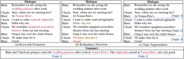
Keywords Extraction aims to automatically identify important words in the dialogue (shown in Figure 1(a)). Our DialoGPT annotator extracts unpredictable words as keywords. We assume that keywords contain high information, which are difficult to be predicted considering both background knowledge encoded in the DialoGPT and contextual information of dialogue context. Redundancy Detection aims to detect redundant utterances that have no core contribution to the overall meaning of the dialogue (shown in Figure 1(b)). Our DialoGPT annotator detects utterances that are useless for dialogue context representation as redundant. We assume that if adding a new utterance does not change the dialogue context representation, then this utterance has no effect on predicting the response, so it is redundant. Topic Segmentation aims to divide a dialogue into topically coherent segments (shown in Figure 1(c)). Our DialoGPT annotator inserts a topic segmentation point before one utterance if it is unpredictable. We assume that if an utterance is difficult to be inferred from the dialogue context based on DialoGPT, this utterance may belong to a new topic.

We use our DialoGPT annotator to annotate the SAMSum Gliwa et al. (2019) and AMI Carletta et al. (2005) datasets. Each annotation is converted into a specific identifier and we insert them into the dialogue text. Then, we employ pre-traind BART Lewis et al. (2020) and non pre-trained PGN See et al. (2017) as our summarizers. Extensive experimental results show that our method can obtain consistent and remarkable improvements over strong baselines on both datasets and achieves new state-of-the-art performance on the SAMSum dataset.

2 Preliminaries

In this section, we will describe the task definition as well as the background of DialoGPT.

2.1 Task Definition

Given an input dialogue ${\mathcal{D}}$, a dialogue summarizer aims to produce a condensed summary ${\mathcal{S}}$, where ${\mathcal{D}}$ consists of $|{\mathcal{D}}|$ utterances $[u_{1},u_{2},...u_{|{\mathcal{D}}|}]$ and ${\mathcal{S}}$ consists of $|{\mathcal{S}}|$ words $[s_{1},s_{2},...s_{|{\mathcal{S}}|}]$. Each utterance $u_{i}$ is compose of a sequence of words $[u_{i,1},u_{i,2},...u_{i,|u_{i}|},\texttt{EOS}_{i}]$, where $i\in[1:|{\mathcal{D}}|]$ and $\texttt{EOS}_{i}$ indicates the end of the utterance. Besides, each utterance $u_{i}$ associates with a speaker $p_{i}$. Thus, this task can be formalized as producing the summary ${\mathcal{S}}$ given the dialogue sequence: $\mathcal{D}=[p_{1},u_{1,1},...,\texttt{EOS}_{1},...,p_{|\mathcal{D}|},u_{|\mathcal{D}|,1},...,\texttt{EOS}_{|\mathcal{D}|}]$

Figure 2: Illustration of our DialoGPT annotator. (I) Given one dialogue, we preprocess it into two formats: context-response pairs and the dialogue sequence. (II) We input them into the DialoGPT, after the forward pass, we can get the word-level and utterance-level predicted losses and representations for dialogue context. (III) We perform three annotation tasks: keywords extraction, redundancy detection and topic segmentation. Finally, we can get a labelled dialogue. #KEY#, [RD] and [TS] are specific tags, which are inserted into the dialogue.

2.2 DialoGPT

DialoGPT Zhang et al. (2020b) is a neural conversational response generation model, which inherits from GPT-2 Radford et al. (2019) and is trained on 147M conversation-like exchanges extracted from Reddit comment chains. There are 3 different sizes of the model with total parameters of 117M, 345M and 762M respectively. It achieves state-of-the-art results over various dialogue generation benchmarks. Given the dialogue context $u_{i-1}=[u_{i-1,1},...,u_{i-1,|u_{i-1}|},\texttt{EOS}_{i-1}]$, DialoGPT aims to produce the response $u_{i}=[u_{i,1},...,u_{i,|u_{i}|},\texttt{EOS}_{i}]$, which can be formalized as the conditional probability of $P(u_{i}|u_{i-1})$. It first takes the context word sequence of no more than 1024 tokens and outputs the representation of the sequence $h_{i}=({\boldsymbol{\mathit{h}}}_{i-1,1},...,{\boldsymbol{\mathit{h}}}_{i-1,|u_{i-1}|},{\boldsymbol{\mathit{h}}}_{i-1,\texttt{EOS}_{i-1}})$, where ${\boldsymbol{\mathit{h}}}_{i-1,\texttt{EOS}_{i-1}}$ can be viewed as the representation of dialogue context $u_{i-1}$. Then, DialoGPT starts decoding the response by attending to the context token representations and partially decoded response tokens until reaching EOS. The loss function is the negative log-likelihood of the response word sequence ${\mathcal{L}}_{DialoGPT}=-\sum_{t=1}^{|u_{i}|}\log p\left(u_{i,t}|u_{i,1}\ldots u_{i,t-1},u_{i-1}\right)$. It’s worth noting that DialoGPT tokenizes texts with the same byte-pair encoding as GPT-2, thus either context or response tokens are tokenized into subwords.

3 Method

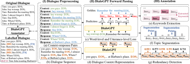
In this section, we will first introduce our DialoGPT annotator. The workflow consists of three steps (1) dialogue preprocessing; (2) DialoGPT forward passing; (3) annotation. The overall framework is shown in Figure 2. Then, we will describe our dialogue summarizer, including BART and PGN.

3.1 Dialogue Preprocessing

Dialogue preprocessing aims to transform the original dialogue $\mathcal{D}=[p_{1},u_{1,1},...,\texttt{EOS}_{1},...,p_{|\mathcal{D}|},u_{|\mathcal{D}|,1},...,\texttt{EOS}_{|\mathcal{D}|}]$ into the format that DialoGPT can process.

Specifically, we transform it into two formats. The first one is context-response pairs (shown in Figure 2(a)). Given a dialogue $\mathcal{D}$, two adjacent utterances $(u_{i-1},u_{i})$ are combined into a context-response pair, where $i\in[2:|\mathcal{D}|]$ . The second one is dialogue sequence (shown in Figure 2(b)). All the utterances in the dialogue $\mathcal{D}$ are serialized into a sequence $[u_{1,1},...,\texttt{EOS}_{1},...,u_{|\mathcal{D}|,1},...,\texttt{EOS}_{|\mathcal{D}|}]$, with EOS separates each utterance.

Note that either for context-response pairs or the dialogue sequence, we do not take speaker information $p$ into consideration. The reason is that DialoGPT is trained on a huge volume of conversational data without speaker information. Even so, Zhang et al. (2020b) proved that DialoGPT can simulate real-world dialogues in various scenes and has already learned diverse response generation patterns between the same speakers or different speakers according to the given context.

3.2 DialoGPT Forward Passing

DialoGPT forward passing has two purposes. (1) For each context-response pair, we aim to get the word-level and utterance-level predicted losses for the response (shown in Figure 2(c)). (2) For the dialogue sequence, we aim to get the representations for each EOS (shown in Figure 2(d)).

For the first purpose, given one context-response pair $(u_{i-1},u_{i})$, we input the context words $u_{i-1}=[u_{i-1,1},u_{i-1,2},...,u_{i-1,|u_{i-1}|},\texttt{EOS}_{i-1}]$ into the DialoGPT and start to decode the response. At each decode step $t$, we calculate the negative log-likelihood between the predicted distribution and the golden target from the given response.

$$\begin{split}&loss_{i,t}=-\log p\left(u_{i,t}|{u_{i,<t}},u_{i-1}\right)\\ &loss_{i}=\frac{1}{|u_{i}|+1}\sum_{t=1}^{|u_{i}|+1}loss_{i,t}\end{split}$$ (1)

where $loss_{i,t}$ and $loss_{i}$ are the predicted losses for each word and each utterance respectively.

For the second purpose, after the single forward pass of DialoGPT over the dialogue sequence, we can get representations $\boldsymbol{\mathit{H}}$ for each token on the top of the DialoGPT. Afterward, we extract all representations for each EOS.

$$\begin{split}&\boldsymbol{\mathit{h}}_{\texttt{EOS}_{1}},\boldsymbol{\mathit{h}}_{\texttt{EOS}_{2}},...,\boldsymbol{\mathit{h}}_{\texttt{EOS}_{|\mathcal{D}|}}=\boldsymbol{\mathit{H}}(\texttt{EOS})\end{split}$$ (2)

where each $\boldsymbol{\mathit{h}}_{\texttt{EOS}_{i}}$ can be viewed as the representation for the dialogue context $[u_{1},...,u_{i}]$.

3.3 Annotation

Figure 3: Illustration of redundancy detection process. The initial redundant utterances set is $\emptyset$. $\boldsymbol{\mathit{h}}_{\texttt{EOS}_{i}}$ is the representation for dialogue context covering the first $i$ utterances. We detect redundant utterances based on the cosine similarity between representations of dialogue context. For example, the similarity score between $\boldsymbol{\mathit{h}}_{\texttt{EOS}_{4}}$ and $\boldsymbol{\mathit{h}}_{\texttt{EOS}_{5}}$ exceeds the pre-defined threshold ($t_{{\textsc{Rd}}}$ is 0.99), which means adding utterance $u_{5}$ into the dialogue context brings little information, thus the utterance $u_{5}$ is detected as redundant.

3.3.1 Keywords Extraction: $\text{DialoGPT}_{{\textsc{Ke}}}$

Motivation Considering both background knowledge encoded in the DialoGPT and contextual information of the dialogue context, if one word in the golden response is difficult to be inferred from DialoGPT, we assume that it contains high information and can be viewed as a keyword.

Given a dialogue $\mathcal{D}$, we have loss $loss_{i,j}$ for each word $u_{i,j}$, where $i\in[2:|\mathcal{D}|]$. We extract $r_{{\textsc{Ke}}}$ percent of words with the highest loss as keywords, where $r_{{\textsc{Ke}}}$ is a hyper-parameter. Moreover, the names of all speakers $\mathbb{P}$ mentioned in the dialogue are also added into the keywords set. Finally, we append a specific tag #KEY# and the keywords to the end of the original dialogue $\mathcal{D}$. The new dialogue with keywords annotation is $\mathcal{D}_{{\textsc{Ke}}}=[\underbrace{p_{1},u_{1,1},...,}_{\mathcal{D}}\underbrace{\texttt{\#KEY\#},\mathbb{P},\texttt{Key}_{1},\texttt{Key}_{2},...}_{keywords}]$.

3.3.2 Redundancy Detection: $\text{DialoGPT}_{{\textsc{Rd}}}$

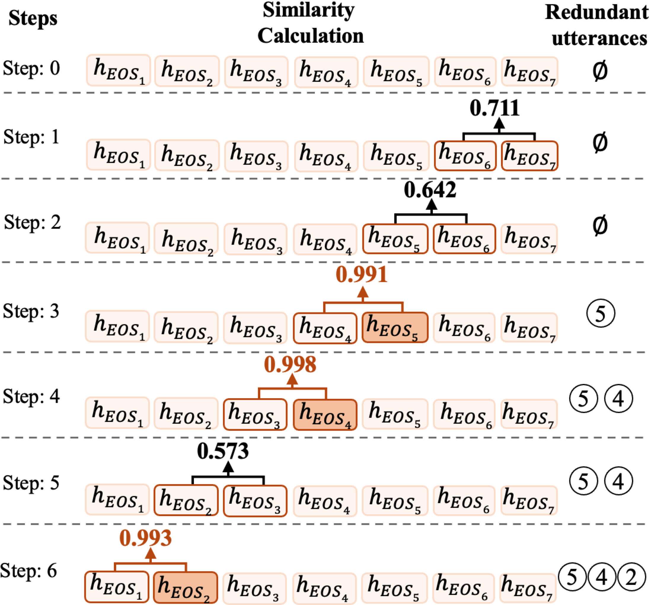
Motivation DialoGPT inherits a decoder architecture, where one token attends to all previous tokens to aggregate information. Thus, given the representation $\boldsymbol{\mathit{h}}_{\texttt{EOS}_{i}}$ for each $\texttt{EOS}_{i}$, it can be viewed as the representation for the dialogue context $[u_{1},u_{2},...,u_{i}]$. Adding a new utterance $u_{i+1}$, if the new context representation $\boldsymbol{\mathit{h}}_{\texttt{EOS}_{i+1}}$ is similar to the previous $\boldsymbol{\mathit{h}}_{\texttt{EOS}_{i}}$, we assume that the new utterance $u_{i+1}$ brings little information and has small effects on predicting the response, thus $u_{i+1}$ becomes a redundant utterance.

We start with the last two dialogue context representations $\boldsymbol{\mathit{h}}_{\texttt{EOS}_{|\mathcal{D}|-1}}$ and $\boldsymbol{\mathit{h}}_{\texttt{EOS}_{|\mathcal{D}|}}$, and calculate the cosine similarity between them. If the similarity score exceeds the threshold $t_{{\textsc{Rd}}}$, the utterance $u_{|\mathcal{D}|}$ is detected as redundant. $t_{{\textsc{Rd}}}$ is a hyper-parameter. If the similarity score doesn’t exceed the threshold $t_{{\textsc{Rd}}}$, we move forward one step to calculate the similarity between $\boldsymbol{\mathit{h}}_{\texttt{EOS}_{|\mathcal{D}|-2}}$ and $\boldsymbol{\mathit{h}}_{\texttt{EOS}_{|\mathcal{D}|-1}}$, and repeat the process until reaching $\boldsymbol{\mathit{h}}_{\texttt{EOS}_{1}}$. An example is shown in Figure 3.

We insert a specific tag [RD] before each redundant utterance. For example, if utterance $u_{1}$ is redundant, the new dialogue with redundant utterances annotation is $\mathcal{D}_{{\textsc{Rd}}}=[p_{1},\texttt{[RD]},u_{1,1},...,\texttt{EOS}_{1},...,p_{|\mathcal{D}|},...,\texttt{EOS}_{|\mathcal{D}|}]$.

3.3.3 Topic Segmentation: $\text{DialoGPT}_{{\textsc{Ts}}}$

Motivation DialoGPT is skilled in generating the context-consistent response. Therefore, if the response is difficult to be predicted given the context based on DialoGPT, we assume the response may belong to another topic and there is a topic segmentation between the context and response.

Given a dialogue $\mathcal{D}$, we have loss $loss_{i}$ for each utterance $u_{i}$, where $i\in[2:|\mathcal{D}|]$. We select $r_{{\textsc{Ts}}}$ percent of utterances with the highest loss as topic segmentation points. $r_{{\textsc{Ts}}}$ is a hyper-parameter. Before each selected utterance, we insert a specific tag [TS]. For example, if there is a segmentation point between utterance $u_{1}$ and utterance $u_{2}$, the new dialogue with topic annotation is $\mathcal{D}_{{\textsc{Ts}}}=[p_{1},u_{1,1},...,\texttt{EOS}_{1},\texttt{[TS]},p_{2},u_{2,1},...,\texttt{EOS}_{2},...]$.

3.4 Summarizer

We employ two kinds of summarizer, one is BART Lewis et al. (2020), which is a Transformer-based model and pre-trained on a huge volume of data. The other one is PGN See et al. (2017), which is a LSTM-based model. Both models inherit a typical sequence-to-sequence framework, which first encodes the source dialogue $\mathcal{D}$ to distributed representations and then generates the target summary $\mathcal{S}$ with the decoder.

BART

BART adopts the Transformer Vaswani et al. (2017) as the backbone architecture. It first map the source dialogue into distributed representations, based on which a decoder generates the target sequence:

$$\begin{split}\boldsymbol{\mathit{X}}^{N}&=\textsc{{Encoder}}(\boldsymbol{\mathit{X}}^{0})\stackrel{{\scriptstyle N}}{{\underset{n=1}{:=}}}\textsc{Ffn}\left(\textsc{Att}(\boldsymbol{\mathit{X}}^{n-1})\right)\\ \boldsymbol{\mathit{Y}}^{M}&=\textsc{{Decoder}}(\boldsymbol{\mathit{Y}}^{0},\boldsymbol{\mathit{X}}^{N})\\ &\stackrel{{\scriptstyle M}}{{\underset{m=1}{:=}}}\textsc{Ffn}\left(\textsc{Att}\left(\textsc{Att}(\boldsymbol{\mathit{Y}}^{m-1}),\boldsymbol{\mathit{X}}^{N}\right)\right)\end{split}$$ (3)

where $\stackrel{{\scriptstyle N}}{{\underset{n=1}{:=}}}$ denotes $N$ identical encoding layers, $\stackrel{{\scriptstyle M}}{{\underset{m=1}{:=}}}$ denotes $M$ identical decoding layers, $\boldsymbol{\mathit{X}}^{0}$ denotes the sum of the word embeddings $\boldsymbol{\mathit{X}}_{\mathrm{emb}}$ and position embeddings $\boldsymbol{\mathit{X}}_{\mathrm{pos}}$ of $\mathcal{D}$, $\boldsymbol{\mathit{Y}}^{0}$ denotes that of the shifted right $\mathcal{S}$, $\textsc{Ffn}(\cdot)$ denotes a position-wise feed-forward network, and $\textsc{Att}(\cdot)$ denotes a multi-head attention. Residual connection (He et al., 2016) and layer normalization (Ba et al., 2016) are used in each sub-layer, which are suppressed in Equation 3 for clarity. Finally, the output representation $\boldsymbol{\mathit{Y}}^{M}$ of the decoder is projected into the vocabulary space and the decoder outputs the highest probability token.

PGN

PGN is a hybrid model of the typical Seq2Seq Attention model Nallapati et al. (2016) and Pointer-Network Vinyals et al. (2015). The input dialogue is fed into the LSTM encoder token by token, producing the encoder hidden states. The decoder receives word embedding of the previous word and generates a distribution to decide the target token, retaining decoder hidden states. PGN not only allows to generate from the fixed vocabulary, but also allows to copy from the input tokens.

Training Objective

Model parameters $\theta$ are trained to maximize the conditional likelihood of the outputs in a parallel training corpus $({\mathbb{D}},{\mathbb{S}})$:

$$\arg\max_{\theta}\sum_{(\mathcal{D},\mathcal{S})\in(\mathbb{D},\mathbb{S})}\log p(\mathcal{S}\,|\,\mathcal{D};\theta).$$ (4)

4 Experiments

		Train	Valid	Test
SAMSum	#	14732	818	819
	Avg.Turns	11.13	10.72	11.24
	Avg.Tokens	120.26	117.46	122.71
	Avg.Sum	22.81	22.80	22.47
AMI	#	97	20	20
	Avg.Turns	310.23	345.70	324.40
	Avg.Tokens	4859.52	5056.25	5257.80
	Avg.Sum	323.74	321.25	328.20

Table 1: Statistics for SAMSum and AMI datasets. “#” means the number of dialogue-summary pairs, “Avg.Turns”, “Avg.Tokens” and “Avg.Sum” mean the average number of turns of dialogues, tokens of dialogues and tokens of summaries respectively.

4.1 Datasets

We experiment on 2 datasets (statistics in Table 1):

SAMSum Gliwa et al. (2019) is a human-generated dialogue summary dataset, which contains dialogues in various scenes of the real-life.

AMI Carletta et al. (2005) is a meeting summary dataset. Each meeting contains four participants and is about a remote control design project.

4.2 Implementation Details

DialoGPT We initialize DialoGPT with DialoGPT-large. For SAMSum, we set keywords extraction ratio $r_{{\textsc{Ke}}}$ to 15, similarity threshold $t_{{\textsc{Rd}}}$ to 0.99 and topic segmentation ratio $r_{{\textsc{Ts}}}$ to 15. For AMI, $r_{{\textsc{Ke}}}$ is 4, $t_{{\textsc{Rd}}}$ is 0.95 and $r_{{\textsc{Ts}}}$ is 5 .

BART We initialize BART with bart.large . For fine-tuning on SAMSum, the learning rate is set to 3e-05, the dropout rate is 0.1, the warmup is set to 400. At the test process, beam size is 5, minimum decoded length is 5 and maximum length is 100.

PGN The word embedding size is set to 300 and initialized with the pre-trained GloVe vector. The dimension of encoder and pointer decoder is set to 200. The dropout is set to 0.5. The learning rate is 0.001. At the test process, beam size is 10, minimum decoded length is 280 and maximum length is 450.

Model	R-1	R-2	R-L
Extractive
LONGEST-3	32.46	10.27	29.92
TextRank	29.27	8.02	28.78
Abstractive
Transformer	36.62	11.18	33.06
D-HGN	42.03	18.07	39.56
TGDGA	43.11	19.15	40.49
DialoGPT	39.77	16.58	38.42
MV-BART	53.42	27.98	$\textbf{49.97}^{\dagger\dagger}$
Ours
BART	52.98	27.67	49.06
[1pt/3pt] BART($\mathcal{D}_{{\textsc{Ke}}}$)	$\textbf{53.43}^{\dagger\dagger}$	$\textbf{28.03}^{\dagger\dagger}$	49.93
BART($\mathcal{D}_{{\textsc{Rd}}}$)	53.39	28.01	49.49
BART($\mathcal{D}_{{\textsc{Ts}}}$)	53.34	27.85	49.64
[1pt/3pt] BART($\mathcal{D}_{{\textsc{All}}}$)	$\textbf{53.70}^{\dagger}$	$\textbf{28.79}^{\dagger}$	$\textbf{50.81}^{\dagger}$

Table 2: Test set results on the SAMSum dataset, where “R” is short for “ROUGE”. BART means fine-tuning BART on the original SAMSum. BART($\mathcal{D}_{{\textsc{Ke}}}$), BART($\mathcal{D}_{{\textsc{Rd}}}$) and BART($\mathcal{D}_{{\textsc{Ts}}}$) represent fine-tuning BART on the SAMSum with keywords, redundancy and topic annotation respectively. $\mathcal{D}_{{\textsc{All}}}$ means the SAMSum with all three annotations. $\dagger$ and $\dagger\dagger$ indicate the first-ranked and second-ranked results respectively.

Model	R-1	R-2	R-L
Extractive
TextRank	35.19	6.13	15.70
SummaRunner	30.98	5.54	13.91
Abstractive
UNS	37.86	7.84	13.72
TopicSeg	$\textbf{51.53}^{\dagger\dagger}$	12.23	$\textbf{25.47}^{\dagger}$
HMNet	$\textbf{52.36}^{\dagger}$	$\textbf{18.63}^{\dagger}$	24.00
Ours
PGN	48.34	16.02	23.49
[1pt/3pt] PGN($\mathcal{D}_{{\textsc{Ke}}}$)	50.22	17.74	24.11
PGN($\mathcal{D}_{{\textsc{Rd}}}$)	50.62	16.86	24.27
PGN($\mathcal{D}_{{\textsc{Ts}}}$)	48.59	16.07	24.05
[1pt/3pt] PGN($\mathcal{D}_{{\textsc{All}}}$)	50.91	$\textbf{17.75}^{\dagger\dagger}$	$\textbf{24.59}^{\dagger\dagger}$

Table 3: Test set results on the AMI dataset. PGN($\mathcal{D}_{{\textsc{Ke}}}$), PGN($\mathcal{D}_{{\textsc{Rd}}}$) and PGN($\mathcal{D}_{{\textsc{Ts}}}$) represent training PGN on the AMI with keywords, redundancy and topic annotation respectively.

SAMSum		AMI
Model	BS	Model	BS
BART	86.91	PGN	80.51
MV-BART	88.46	HMNet	82.24
BART($\mathcal{D}_{{\textsc{All}}}$)	90.04	PGN($\mathcal{D}_{{\textsc{All}}}$)	82.76

Table 4: Test set results on the SAMSum and AMI. “BS” is short for BERTScore.

4.3 Baselines and Metrics

For SAMSum, LONGEST-3 views the first three utterances as the summary. TextRank Mihalcea and Tarau (2004) is a traditional graph-based method. Transformer Vaswani et al. (2017) is a seq2seq method based on full self-attention operations. D-HGN Feng et al. (2020a) incorporates commonsense knowledge to help understand dialogues. TGDGA Zhao et al. (2020) uses topic words and models graph structures for dialogues. DialoGPT Zhang et al. (2020b) means that fine-tuning DialoGPT on the SAMSum. MV-BART Chen and Yang (2020) is a BART-based method that incorporates topic and stage information.

For AMI, SummaRunner Nallapati et al. (2017) is an extractive method based on hierarchical RNN network. UNS Shang et al. (2018) is a fully unsupervised and graph-based method. TopicSeg Li et al. (2019) incorporates topics to model the meeting. HMNet Zhu et al. (2020) is a transformer-based method that incorporates POS and entity information and is pre-trained on news summarization dataset.

We adopt ROUGE Lin (2004) and BERTScore Zhang et al. (2020a) for evaluating our models.

4.4 Automatic Evaluation

The results on SAMSum and AMI are shown in Table 2 and 3 respectively. We can see that using our annotated datasets $\mathcal{D}_{{\textsc{Ke}}}$, $\mathcal{D}_{{\textsc{Rd}}}$ and $\mathcal{D}_{{\textsc{Ts}}}$, both BART and PGN can obtain improvements. Furthermore, our BART($\mathcal{D}_{{\textsc{All}}}$) achieves SOTA performance.

For SAMSum, it’s worth noting that BART($\mathcal{D}_{{\textsc{Ke}}}$) performs better compared with BART($\mathcal{D}_{{\textsc{Rd}}}$) and BART($\mathcal{D}_{{\textsc{Ts}}}$). We attribute this to the fact that keywords can retain essential information for shorter dialogues. For AMI, PGN($\mathcal{D}_{{\textsc{Rd}}}$) contributes the most, which shows the importance of detecting redundancy in verbose meeting transcripts. Although HMNet and TopicSeg achieve better scores, HMNet needs news summarization dataset to pre-train the model and TopicSeg designs complex attention mechanism to incorporate topic information.

In terms of new embedding-based metric BERTScore (shown in Table 4), our method BART($\mathcal{D}_{{\textsc{All}}}$) and PGN($\mathcal{D}_{{\textsc{All}}}$) can consistently outperform the baseline models.

4.5 Human Evaluation

	Model	Info.	Conc.	Cov.
SAMSum	Golden	4.37	4.26	4.27
2-5	BART	3.66	3.65	3.66
	MV-BART	3.85	3.76	3.88
	BART($\mathcal{D}_{{\textsc{Ke}}}$)	3.88	3.77	3.79
	BART($\mathcal{D}_{{\textsc{Rd}}}$)	3.74	$\textbf{3.98 }^{\dagger}$	3.89
	BART($\mathcal{D}_{{\textsc{Ts}}}$)	$\textbf{3.95}^{\dagger\dagger}$	3.76	$\textbf{4.01}^{\dagger\dagger}$
	BART($\mathcal{D}_{{\textsc{All}}}$)	$\textbf{4.05}^{\dagger}$	$\textbf{3.78}^{\dagger\dagger}$	$\textbf{4.08}^{\dagger}$
AMI	Golden	4.70	3.85	4.35
2-5	PGN	2.92	3.08	2.70
	HMNet	$\textbf{3.52}^{\dagger}$	2.40	$\textbf{3.40}^{\dagger}$
	PGN($\mathcal{D}_{{\textsc{Ke}}}$)	3.20	3.08	3.00
	PGN($\mathcal{D}_{{\textsc{Rd}}}$)	3.15	$\textbf{3.25}^{\dagger}$	3.00
	PGN($\mathcal{D}_{{\textsc{Ts}}}$)	3.05	$\textbf{3.10}^{\dagger\dagger}$	$\textbf{3.17}^{\dagger\dagger}$
	PGN($\mathcal{D}_{{\textsc{All}}}$)	$\textbf{3.33}^{\dagger\dagger}$	$\textbf{3.25}^{\dagger}$	3.10

Table 5: Human evaluation results. “Info.” is short for informativeness, “Conc.” for conciseness, “Cov.” for coverage. For SAMSum, the inter-annotator agreement (Fleiss’ kappa) scores for each metric are 0.46, 0.37 and 0.43 respectively. For AMI, Fleiss’ kappa scores are 0.48, 0.40 and 0.41 respectively.

We conduct a human evaluation of the dialogue summary to assess its informativeness, conciseness and coverage. Informativeness measures how well the summary includes key information. Conciseness measures how well the summary discards the redundant information. Coverage measures how well the summary covers each part of the dialogue.

We randomly sample 100 dialogues (SAMSum) and 10 meetings (AMI) with corresponding generated summaries to conduct the evaluation. In order to reduce variance caused by humans, we have 4 human evaluators and they were asked to rate each summary on a scale of 1 to 5 (higher is better) for each metric. The results are shown in Table 5.

We can see that our method can achieve higher scores in all three metrics. Especially, combined with $\mathcal{D}_{{\textsc{Rd}}}$, our model can get the best score in conciseness. Besides, combined with $\mathcal{D}_{{\textsc{Ts}}}$, our model can perform better in coverage. However, HMNet gets the best score in informativeness and coverage. We argue this is because HMNet forces a minimum summary length of 400. Due to this, it scores the worst in conciseness. For the AMI, we also find there is still a gap between the scores of generated summaries and the scores of golden summaries, indicating that the AMI is more difficult.

4.6 Analysis

Effect of $\text{DialoGPT}_{{\textsc{Ke}}}$.

Method	R-1	R-2	R-L
Rule-Based Methods
Entities	53.36	27.71	49.69
Nouns and Verbs	52.75	27.48	48.82
Traditional Methods
TextRank	53.29	27.66	49.33
Topic words	53.28	27.76	49.59
Pre-trained Language Model-Based Methods
KeyBERT
w/ BERT emb	52.39	27.14	48.52
w/ DialoGPT emb	53.14	27.25	49.42
Ours
$\text{DialoGPT}_{{\textsc{Ke}}}$	53.43	28.03	49.93

Table 6: Test set results of fine-tuning BART on the SAMSum that is annotated with keywords using various methods. Entities, nouns and verbs are obtained by Qi et al. (2020). Topic words are obtained by a pre-trained LDA model Narayan et al. (2018). KeyBERT Grootendorst (2020) leverages pre-trained language model embeddings to create keywords.

Method	Precision	Recall	$\mathbf{F_{1}}$
TextRank	47.74%	17.44%	23.22%
Entities	60.42%	17.80%	25.38%
$\text{DialoGPT}_{{\textsc{Ke}}}$	33.20%	29.49%	30.31%

Table 7: Quantitative evaluation for keywords on SAMSum test set by viewing reference summary words as golden keywords.

To verify the effectiveness of our $\text{DialoGPT}_{{\textsc{Ke}}}$ method, we fine-tune BART on SAMSum, which is annotated by various keywords extraction methods. The results are shown in Table 6. We can see that our method achieves higher scores. The results also show that entities play an important role in the summary generation. Besides, combined with DialoGPT embeddings, KeyBERT can get better results.

To give a quantitative evaluation, we view reference summary words as golden keywords and calculate the precision, recall and $F_{1}$ scores for extracted keywords. The results are shown in Table 7. Directly using entities as keywords can get the best precision score. However, both TextRank and Entities perform poorly in recall. Our method gets the best score in terms of $F_{1}$ and its advantage is mainly reflected in recall score, which shows our method can extract more diverse keywords.

Effect of $\text{DialoGPT}_{{\textsc{Rd}}}$.

Model	R-1	R-2	R-L
SAMSum
Rule-based	53.00	27.71	49.68
$\text{DialoGPT}_{{\textsc{Rd}}}$	53.39	28.01	49.49
AMI
Rule-based	50.19	16.45	23.95
$\text{DialoGPT}_{{\textsc{Rd}}}$	50.62	16.86	24.27

Table 8: Test set results on the SAMSum and AMI datasets that are annotated with redundant utterances. “Rule-based” indicates annotating utterances that contain no noun, verb and adjective as redundant.

To verify the effectiveness of our $\text{DialoGPT}_{{\textsc{Rd}}}$ method, we compare it with a Rule-based method Dinarelli et al. (2009), which annotates utterances without noun, verb and adjective as redundant. The results are shown in Table 8. We can see that our method performs better. Especially, our method shows more advantages for long and verbose meeting transcripts in the AMI.

Effect of $\text{DialoGPT}_{{\textsc{Ts}}}$.

To verify the effectiveness of our $\text{DialoGPT}_{{\textsc{Ts}}}$ method, we compare it with the C99 algorithm Choi (2000), which is a sentence similarity-based segmentation method. Chen and Yang (2020) enhance it with BERT Devlin et al. (2019) embeddings. We further combine the algorithm with DialoGPT embeddings. The results are shown in Table 9. We can see that our method can get comparable results with the strong baseline C99(w/ DialoGPT emb). For AMI, combined with golden topic annotation, PGN can achieve the best result, which shows modeling topics is an essential task for dialogue summarization.

Model	R-1	R-2	R-L
SAMSum
C99
w/ BERT emb	52.80	27.78	49.50
w/ DialoGPT emb	53.33	28.04	49.39
$\text{DialoGPT}_{{\textsc{Ts}}}$	53.34	27.85	49.64
AMI
Golden	50.28	19.73	24.45
[1pt/3pt] C99
w/ BERT emb	48.53	15.84	23.63
w/ DialoGPT emb	49.22	16.79	23.88
$\text{DialoGPT}_{{\textsc{Ts}}}$	48.59	16.07	24.05

Table 9: Test set results on SAMSum and AMI that are annotated with topic segmentation in various methods. C99 Choi (2000) segments dialogues based on inter-sentence similarities. Beside, the AMI has golden topic segmentation annotations.

4.7 Case Study

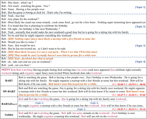
Figure 4 shows summaries generated by different models for an example dialogue in the SAMSum dataset. We can see that BART Lewis et al. (2020) tends to generate long and redundant summaries. By incorporating topic and stage information, MV-BART Chen and Yang (2020) can generate summaries that cover main topics of the dialogue. However, it still suffers from redundancy problem. Our BART($\mathcal{D}_{{\textsc{All}}}$) can get higher ROUGE scores while generating better summaries. The generated summary can include extracted keywords and correspond to each topic of the dialogue. We also find that even some redundant utterances have already been detected, our model still generate the summary contains some redundant information. We attribute this to the fact that the small dataset leads to insufficient training of the model.

5 Related Work

Dialogue Summarization Current works mainly incorporate auxiliary information to help better modeling dialogues. Some works used various types of keywords to identify the core part of the dialogue, including entities Zhu et al. (2020), domain terminologies Koay et al. (2020) and topic words Zhao et al. (2020). Some works aimed to reduce redundancy, Zechner (2002); Murray et al. (2005) used sentence-level similarity-based methods. Some works incorporate topics as a coarse-grained dialogue structure Li et al. (2019); Liu et al. (2019); Chen and Yang (2020). Other works also explored dialogue act Goo and Chen (2018), dialogue discourse Feng et al. (2020b) and commonsense knowledge Feng et al. (2020a). In this paper, we combine three types of auxiliary information to help better modeling dialogues, including keywords, redundant utterances and topics.

Figure 4: Example dialogue in the SAMSum dataset and summaries generated by different models. Keyowrds, redundant utterances and topics are annotated by our DialoGPT Annotator. “R” is short for ROUGE. Our model BART($\mathcal{D}_{{\textsc{All}}}$) can get higher ROUGE scores while generating the better summary.

Pre-trained Language Models Pre-trained models such as BERT Devlin et al. (2019) and GPT-3 Brown et al. (2020) have advanced various NLP tasks. On one hand, some works utilized the knowledge contained in pre-trained models by fine-tuning on supervised data of downstream tasks Qin et al. (2019); Liu and Lapata (2019); Qin et al. (2020). On the other hand, some works examined the knowledge in an unsupervised manner Jiang et al. (2020); Xiao et al. (2020); Lin et al. (2020). Kumar et al. (2020) explored pre-trained models for conditional data augmentation. Wang et al. (2020) used the knowledge in pre-trained models to construct knowledge graphs. In this paper, we belong to the second paradigm and propose our DialoGPT annotator that can perform three annotation tasks in an unsupervised manner.

6 Conclusion

We investigate to use DialoGPT as unsupervised annotators for dialogue summarization, including keywords extraction, redundancy detection and topic segmentation. We conduct our DialoGPT annotator on two datasets, SAMSum and AMI. Experimental results show that our method consistently obtains improvements upon pre-traind summarizer (BART) and non pre-trained summarizer (PGN) on both datasets. Besides, combining all three annotations, our summarizer can achieve new state-of-the-art performance on the SAMSum dataset.

Appendix A Evaluation Details

For ROUGE Lin (2004), we employ Py-rouge package to evaluate our models following Gliwa et al. (2019). For BERTScore Zhang et al. (2020a), we use the official implementation to evaluate our models. The detailed command line for BERTScore is bert-score -r golden.txt -c gen.txt --lang en.

Appendix B Ablation Studies for Annotations

To further verify the effectiveness of our method, we conduct ablation studies for each annotation. The results are shown in Table 10 and Table 11. We can find that: (1) For both datasets, training summarizers based on datasets with two of three annotations can obtain improvements. (2) For both datasets, training summarizers based on datasets with two of three annotations can surpass corresponding summarizers that are trained based on datasets with one type of annotation (e.g., BART($\mathcal{D}_{{\textsc{Ke}}+{\textsc{Rd}}}$) is better than BART($\mathcal{D}_{{\textsc{Ke}}}$) and BART($\mathcal{D}_{{\textsc{Rd}}}$)). (3) Compared with summarizers that are trained on $\mathcal{D}_{{\textsc{Rd}}+{\textsc{Ts}}}$ and $\mathcal{D}_{{\textsc{Ke}}+{\textsc{Rd}}}$, summarizers that are trained on $\mathcal{D}_{{\textsc{Ke}}+{\textsc{Ts}}}$ get relatively small improvements on both datasets. Nevertheless, it indicates that $\text{DialoGPT}_{{\textsc{Ke}}}$ and $\text{DialoGPT}_{{\textsc{Ts}}}$ still have non-overlapping parts. (4) Combining all three annotations, both summarizers can achieve the best results in all ROUGE scores.

Model	R-1	R-2	R-L
Ours
BART	52.98	27.67	49.06
[1pt/3pt] BART($\mathcal{D}_{{\textsc{Ke}}}$)	53.43	28.03	49.93
BART($\mathcal{D}_{{\textsc{Rd}}}$)	53.39	28.01	49.49
BART($\mathcal{D}_{{\textsc{Ts}}}$)	53.34	27.85	49.64
[1pt/3pt] BART($\mathcal{D}_{{\textsc{Ke}}+{\textsc{Rd}}}$)	53.56	28.65	50.55
BART($\mathcal{D}_{{\textsc{Ke}}+{\textsc{Ts}}}$)	53.51	28.13	50.00
BART($\mathcal{D}_{{\textsc{Rd}}+{\textsc{Ts}}}$)	53.64	28.33	50.13
[1pt/3pt] BART($\mathcal{D}_{{\textsc{All}}}$)	53.70	28.79	50.81

Table 10: Test set results on the SAMSum dataset. BART means fine-tuning BART on the original SAMSum. BART($\mathcal{D}_{{\textsc{Ke}}}$), BART($\mathcal{D}_{{\textsc{Rd}}}$) and BART($\mathcal{D}_{{\textsc{Ts}}}$) represent fine-tuning BART on the SAMSum with keywords, redundancy and topic annotation respectively. BART($\mathcal{D}_{{\textsc{Ke}}+{\textsc{Rd}}}$) represent fine-tuning BART on the SAMSum with keywords and redundancy annotations. $\mathcal{D}_{{\textsc{All}}}$ means the SAMSum with all three annotations.

Model	R-1	R-2	R-L
Ours
PGN	48.34	16.02	23.49
[1pt/3pt] PGN($\mathcal{D}_{{\textsc{Ke}}}$)	50.22	17.74	24.11
PGN($\mathcal{D}_{{\textsc{Rd}}}$)	50.62	16.86	24.27
PGN($\mathcal{D}_{{\textsc{Ts}}}$)	48.59	16.07	24.05
[1pt/3pt] PGN($\mathcal{D}_{{\textsc{Ke}}+{\textsc{Rd}}}$)	50.74	17.11	24.52
PGN($\mathcal{D}_{{\textsc{Ke}}+{\textsc{Ts}}}$)	50.69	16.83	24.33
PGN($\mathcal{D}_{{\textsc{Rd}}+{\textsc{Ts}}}$)	50.70	16.96	24.38
[1pt/3pt] PGN($\mathcal{D}_{{\textsc{All}}}$)	50.91	17.75	24.59

Table 11: Test set results on the AMI dataset. PGN($\mathcal{D}_{{\textsc{Ke}}}$), PGN($\mathcal{D}_{{\textsc{Rd}}}$) and PGN($\mathcal{D}_{{\textsc{Ts}}}$) represent training PGN on the AMI with keywords, redundancy and topic annotation respectively. PGN($\mathcal{D}_{{\textsc{Ke}}+{\textsc{Rd}}}$) represent training PGN on the AMI with both keywords and redundancy annotations.

Appendix C Hyper-parameter Search Results

Tables 12 to 17 show the hyper-parameter search results. Finally, for SAMSum Gliwa et al. (2019), we set keywords extraction ratio $r_{{\textsc{Ke}}}$ to 15, similarity threshold $t_{{\textsc{Rd}}}$ to 0.99 and topic segmentation ratio $r_{{\textsc{Ts}}}$ to 15. for AMI Carletta et al. (2005), $r_{{\textsc{Ke}}}$ is 4, $t_{{\textsc{Rd}}}$ is 0.95 and $r_{{\textsc{Ts}}}$ is 5.

Model	$\mathbf{r_{{\textsc{Ke}}}}$	R-1	R-2	R-L
BART($\mathcal{D}_{{\textsc{Ke}}}$)	10	52.17	26.64	48.34
BART($\mathcal{D}_{{\textsc{Ke}}}$)	15	53.43	28.03	49.93
BART($\mathcal{D}_{{\textsc{Ke}}}$)	20	53.20	28.01	49.46
BART($\mathcal{D}_{{\textsc{Ke}}}$)	25	52.78	27.35	48.67

Table 12: Test set results on the SAMSum dataset. BART($\mathcal{D}_{{\textsc{Ke}}}$) means fine-tuning BART on SAMSum with keywords annotation. $r_{{\textsc{Ke}}}$ means different keywords extraction ratios.

Model	$\mathbf{r_{{\textsc{Ke}}}}$	R-1	R-2	R-L
PGN($\mathcal{D}_{{\textsc{Ke}}}$)	3	49.76	16.03	23.64
PGN($\mathcal{D}_{{\textsc{Ke}}}$)	4	50.22	17.74	24.11
PGN($\mathcal{D}_{{\textsc{Ke}}}$)	5	49.63	16.71	23.88
PGN($\mathcal{D}_{{\textsc{Ke}}}$)	6	49.70	16.92	24.42

Table 13: Test set results on the AMI dataset. PGN($\mathcal{D}_{{\textsc{Ke}}}$) means training PGN on AMI with keywords annotation. $r_{{\textsc{Ke}}}$ means different keywords extraction ratios.

Model	$\mathbf{t_{{\textsc{Rd}}}}$	R-1	R-2	R-L
BART($\mathcal{D}_{{\textsc{Rd}}}$)	0.95	52.29	26.71	48.53
BART($\mathcal{D}_{{\textsc{Rd}}}$)	0.96	53.20	27.98	49.68
BART($\mathcal{D}_{{\textsc{Rd}}}$)	0.97	52.17	27.10	48.34
BART($\mathcal{D}_{{\textsc{Rd}}}$)	0.98	53.29	27.89	49.71
BART($\mathcal{D}_{{\textsc{Rd}}}$)	0.99	53.39	28.01	49.49

Table 14: Test set results on the SAMSum dataset. BART($\mathcal{D}_{{\textsc{Rd}}}$) means fine-tuning BART on SAMSum with redundant utterances annotation. $t_{{\textsc{Rd}}}$ means different similarity thresholds.

Model	$\mathbf{t_{{\textsc{Rd}}}}$	R-1	R-2	R-L
PGN($\mathcal{D}_{{\textsc{Rd}}}$)	0.95	50.62	16.86	24.27
PGN($\mathcal{D}_{{\textsc{Rd}}}$)	0.96	49.68	16.54	24.70
PGN($\mathcal{D}_{{\textsc{Rd}}}$)	0.97	50.18	16.12	24.56
PGN($\mathcal{D}_{{\textsc{Rd}}}$)	0.98	48.63	15.17	23.50
PGN($\mathcal{D}_{{\textsc{Rd}}}$)	0.99	47.15	13.94	22.53

Table 15: Test set results on the AMI dataset. PGN($\mathcal{D}_{{\textsc{Rd}}}$) means training PGN on AMI with redundant utterances annotation. $t_{{\textsc{Rd}}}$ means different similarity thresholds.

Model	$\mathbf{r_{{\textsc{Ts}}}}$	R-1	R-2	R-L
BART($\mathcal{D}_{{\textsc{Ts}}}$)	10	53.21	27.38	49.32
BART($\mathcal{D}_{{\textsc{Ts}}}$)	15	53.34	27.85	49.64
BART($\mathcal{D}_{{\textsc{Ts}}}$)	20	52.82	27.34	49.05
BART($\mathcal{D}_{{\textsc{Ts}}}$)	25	53.04	27.49	49.70

Table 16: Test set results on the SAMSum dataset. BART($\mathcal{D}_{{\textsc{Ts}}}$) means fine-tuning BART on SAMSum with topic annotation. $r_{{\textsc{Ts}}}$ means different topic segmentation ratios.

Model	$\mathbf{r_{{\textsc{Ts}}}}$	R-1	R-2	R-L
PGN($\mathcal{D}_{{\textsc{Ts}}}$)	4	49.39	16.02	23.89
PGN($\mathcal{D}_{{\textsc{Ts}}}$)	5	48.59	16.07	24.05
PGN($\mathcal{D}_{{\textsc{Ts}}}$)	6	49.89	16.04	23.01
PGN($\mathcal{D}_{{\textsc{Ts}}}$)	7	49.37	16.07	23.46

Table 17: Test set results on the AMI dataset. PGN($\mathcal{D}_{{\textsc{Ts}}}$) means training PGN on AMI with topic annotation. $r_{{\textsc{Ts}}}$ means different topic segmentation ratios.

References

- Ba et al. (2016) Jimmy Lei Ba, Jamie Ryan Kiros, and Geoffrey E Hinton. 2016. Layer normalization. In arXiv.
- Brown et al. (2020) Tom B. Brown, Benjamin Mann, Nick Ryder, Melanie Subbiah, Jared Kaplan, Prafulla Dhariwal, Arvind Neelakantan, Pranav Shyam, Girish Sastry, Amanda Askell, Sandhini Agarwal, Ariel Herbert-Voss, Gretchen Krueger, Tom Henighan, Rewon Child, Aditya Ramesh, Daniel M. Ziegler, Jeffrey Wu, Clemens Winter, Christopher Hesse, Mark Chen, Eric Sigler, Mateusz Litwin, Scott Gray, Benjamin Chess, Jack Clark, Christopher Berner, Sam McCandlish, Alec Radford, Ilya Sutskever, and Dario Amodei. 2020. Language models are few-shot learners. In Advances in Neural Information Processing Systems 33: Annual Conference on Neural Information Processing Systems 2020, NeurIPS 2020, December 6-12, 2020, virtual.
- Carletta et al. (2005) Jean Carletta, Simone Ashby, Sebastien Bourban, Mike Flynn, Mael Guillemot, Thomas Hain, Jaroslav Kadlec, Vasilis Karaiskos, Wessel Kraaij, Melissa Kronenthal, et al. 2005. The ami meeting corpus: A pre-announcement. In International workshop on machine learning for multimodal interaction. Springer.
- Chen and Yang (2020) Jiaao Chen and Diyi Yang. 2020. Multi-view sequence-to-sequence models with conversational structure for abstractive dialogue summarization. In Proceedings of the 2020 Conference on Empirical Methods in Natural Language Processing (EMNLP), pages 4106–4118, Online. Association for Computational Linguistics.
- Choi (2000) Freddy Y. Y. Choi. 2000. Advances in domain independent linear text segmentation. In 1st Meeting of the North American Chapter of the Association for Computational Linguistics.
- Devlin et al. (2019) Jacob Devlin, Ming-Wei Chang, Kenton Lee, and Kristina Toutanova. 2019. BERT: Pre-training of deep bidirectional transformers for language understanding. In Proceedings of the 2019 Conference of the North American Chapter of the Association for Computational Linguistics: Human Language Technologies, Volume 1 (Long and Short Papers), pages 4171–4186, Minneapolis, Minnesota. Association for Computational Linguistics.
- Dinarelli et al. (2009) Marco Dinarelli, Silvia Quarteroni, Sara Tonelli, Alessandro Moschitti, and Giuseppe Riccardi. 2009. Annotating spoken dialogs: from speech segments to dialog acts and frame semantics. In Proceedings of SRSL 2009, the 2nd Workshop on Semantic Representation of Spoken Language, pages 34–41.
- Feng et al. (2020a) Xiachong Feng, X. Feng, B. Qin, and T. Liu. 2020a. Incorporating commonsense knowledge into abstractive dialogue summarization via heterogeneous graph networks. ArXiv, abs/2010.10044.
- Feng et al. (2020b) Xiachong Feng, Xiaocheng Feng, Bing Qin, and Xinwei Geng. 2020b. Dialogue discourse-aware graph model and data augmentation for meeting summarization.
- Gliwa et al. (2019) Bogdan Gliwa, Iwona Mochol, Maciej Biesek, and Aleksander Wawer. 2019. SAMSum corpus: A human-annotated dialogue dataset for abstractive summarization. In Proceedings of the 2nd Workshop on New Frontiers in Summarization, pages 70–79, Hong Kong, China. Association for Computational Linguistics.
- Goo and Chen (2018) Chih-Wen Goo and Yun-Nung Chen. 2018. Abstractive dialogue summarization with sentence-gated modeling optimized by dialogue acts. 2018 IEEE Spoken Language Technology Workshop (SLT), pages 735–742.
- Grootendorst (2020) Maarten Grootendorst. 2020. Keybert: Minimal keyword extraction with bert.
- Gurevych and Strube (2004) Iryna Gurevych and Michael Strube. 2004. Semantic similarity applied to spoken dialogue summarization. In COLING 2004: Proceedings of the 20th International Conference on Computational Linguistics, pages 764–770, Geneva, Switzerland. COLING.
- He et al. (2016) Kaiming He, Xiangyu Zhang, Shaoqing Ren, and Jian Sun. 2016. Deep residual learning for image recognition. In 2016 IEEE Conference on Computer Vision and Pattern Recognition, CVPR 2016, Las Vegas, NV, USA, June 27-30, 2016, pages 770–778. IEEE Computer Society.
- Jiang et al. (2020) Zhengbao Jiang, Frank F. Xu, Jun Araki, and Graham Neubig. 2020. How can we know what language models know? Transactions of the Association for Computational Linguistics, 8:423–438.
- Koay et al. (2020) Jia Jin Koay, Alexander Roustai, Xiaojin Dai, Dillon Burns, Alec Kerrigan, and Fei Liu. 2020. How domain terminology affects meeting summarization performance. In Proceedings of the 28th International Conference on Computational Linguistics, pages 5689–5695, Barcelona, Spain (Online). International Committee on Computational Linguistics.
- Kumar et al. (2020) Varun Kumar, Ashutosh Choudhary, and Eunah Cho. 2020. Data augmentation using pre-trained transformer models. In Proceedings of the 2nd Workshop on Life-long Learning for Spoken Language Systems, pages 18–26, Suzhou, China. Association for Computational Linguistics.
- Lewis et al. (2020) Mike Lewis, Yinhan Liu, Naman Goyal, Marjan Ghazvininejad, Abdelrahman Mohamed, Omer Levy, Veselin Stoyanov, and Luke Zettlemoyer. 2020. BART: Denoising sequence-to-sequence pre-training for natural language generation, translation, and comprehension. In Proceedings of the 58th Annual Meeting of the Association for Computational Linguistics, pages 7871–7880, Online. Association for Computational Linguistics.
- Li et al. (2019) Manling Li, Lingyu Zhang, Heng Ji, and Richard J. Radke. 2019. Keep meeting summaries on topic: Abstractive multi-modal meeting summarization. In Proceedings of the 57th Annual Meeting of the Association for Computational Linguistics, pages 2190–2196, Florence, Italy. Association for Computational Linguistics.
- Lin et al. (2020) Bill Yuchen Lin, Seyeon Lee, Rahul Khanna, and Xiang Ren. 2020. Birds have four legs?! NumerSense: Probing Numerical Commonsense Knowledge of Pre-Trained Language Models. In Proceedings of the 2020 Conference on Empirical Methods in Natural Language Processing (EMNLP), pages 6862–6868, Online. Association for Computational Linguistics.
- Lin (2004) Chin-Yew Lin. 2004. ROUGE: A package for automatic evaluation of summaries. In Text Summarization Branches Out, pages 74–81, Barcelona, Spain. Association for Computational Linguistics.
- Liu and Lapata (2019) Yang Liu and Mirella Lapata. 2019. Text summarization with pretrained encoders. In Proceedings of the 2019 Conference on Empirical Methods in Natural Language Processing and the 9th International Joint Conference on Natural Language Processing (EMNLP-IJCNLP), pages 3730–3740, Hong Kong, China. Association for Computational Linguistics.
- Liu et al. (2019) Zhengyuan Liu, A. Ng, Sheldon Lee Shao Guang, AiTi Aw, and Nancy F. Chen. 2019. Topic-aware pointer-generator networks for summarizing spoken conversations. 2019 IEEE Automatic Speech Recognition and Understanding Workshop (ASRU), pages 814–821.
- Mihalcea and Tarau (2004) Rada Mihalcea and Paul Tarau. 2004. TextRank: Bringing order into text. In Proceedings of the 2004 Conference on Empirical Methods in Natural Language Processing, pages 404–411, Barcelona, Spain. Association for Computational Linguistics.
- Murray et al. (2005) Gabriel Murray, S. Renals, and J. Carletta. 2005. Extractive summarization of meeting recordings. In INTERSPEECH.
- Nallapati et al. (2017) Ramesh Nallapati, Feifei Zhai, and Bowen Zhou. 2017. Summarunner: A recurrent neural network based sequence model for extractive summarization of documents. In Proceedings of the AAAI Conference on Artificial Intelligence, volume 31.
- Nallapati et al. (2016) Ramesh Nallapati, Bowen Zhou, C. D. Santos, Çaglar Gülçehre, and Bing Xiang. 2016. Abstractive text summarization using sequence-to-sequence rnns and beyond. In CoNLL.
- Narayan et al. (2018) Shashi Narayan, Shay B. Cohen, and Mirella Lapata. 2018. Don’t give me the details, just the summary! Topic-aware convolutional neural networks for extreme summarization. In Proceedings of the 2018 Conference on Empirical Methods in Natural Language Processing, Brussels, Belgium.
- Peyrard (2019) Maxime Peyrard. 2019. A simple theoretical model of importance for summarization. In Proceedings of the 57th Annual Meeting of the Association for Computational Linguistics, pages 1059–1073, Florence, Italy. Association for Computational Linguistics.
- Qi et al. (2020) Peng Qi, Yuhao Zhang, Yuhui Zhang, Jason Bolton, and Christopher D. Manning. 2020. Stanza: A python natural language processing toolkit for many human languages. In Proceedings of the 58th Annual Meeting of the Association for Computational Linguistics: System Demonstrations, pages 101–108, Online. Association for Computational Linguistics.
- Qin et al. (2019) Libo Qin, Wanxiang Che, Yangming Li, Haoyang Wen, and T. Liu. 2019. A stack-propagation framework with token-level intent detection for spoken language understanding. In EMNLP/IJCNLP.
- Qin et al. (2020) Libo Qin, Zhouyang Li, Wanxiang Che, Minheng Ni, and Ting Liu. 2020. Co-gat: A co-interactive graph attention network for joint dialog act recognition and sentiment classification. ArXiv, abs/2012.13260.
- Radford et al. (2019) Alec Radford, Jeffrey Wu, Rewon Child, David Luan, Dario Amodei, and Ilya Sutskever. 2019. Language models are unsupervised multitask learners. OpenAI blog, 1(8):9.
- Riedhammer et al. (2008) K. Riedhammer, B. Favre, and Dilek Z. Hakkani-Tür. 2008. A keyphrase based approach to interactive meeting summarization. 2008 IEEE Spoken Language Technology Workshop, pages 153–156.
- Sainz and Rigau (2021) Oscar Sainz and German Rigau. 2021. Ask2transformers: Zero-shot domain labelling with pre-trained language models.
- See et al. (2017) Abigail See, Peter J. Liu, and Christopher D. Manning. 2017. Get to the point: Summarization with pointer-generator networks. In Proceedings of the 55th Annual Meeting of the Association for Computational Linguistics (Volume 1: Long Papers), pages 1073–1083, Vancouver, Canada. Association for Computational Linguistics.
- Shang et al. (2018) Guokan Shang, Wensi Ding, Zekun Zhang, Antoine Tixier, Polykarpos Meladianos, Michalis Vazirgiannis, and Jean-Pierre Lorré. 2018. Unsupervised abstractive meeting summarization with multi-sentence compression and budgeted submodular maximization. In Proceedings of the 56th Annual Meeting of the Association for Computational Linguistics (Volume 1: Long Papers), pages 664–674, Melbourne, Australia. Association for Computational Linguistics.
- Vaswani et al. (2017) Ashish Vaswani, Noam Shazeer, Niki Parmar, Jakob Uszkoreit, Llion Jones, Aidan N. Gomez, Lukasz Kaiser, and Illia Polosukhin. 2017. Attention is all you need. In Advances in Neural Information Processing Systems 30: Annual Conference on Neural Information Processing Systems 2017, December 4-9, 2017, Long Beach, CA, USA, pages 5998–6008.
- Vinyals et al. (2015) Oriol Vinyals, Meire Fortunato, and Navdeep Jaitly. 2015. Pointer networks. In Advances in Neural Information Processing Systems 28: Annual Conference on Neural Information Processing Systems 2015, December 7-12, 2015, Montreal, Quebec, Canada, pages 2692–2700.
- Wang et al. (2020) C. Wang, Xiao Liu, and D. Song. 2020. Language models are open knowledge graphs. ArXiv, abs/2010.11967.
- Xiao et al. (2020) Liqiang Xiao, Lu Wang, Hao He, and Yaohui Jin. 2020. Modeling content importance for summarization with pre-trained language models. In Proceedings of the 2020 Conference on Empirical Methods in Natural Language Processing (EMNLP), pages 3606–3611, Online. Association for Computational Linguistics.
- Zechner (2002) Klaus Zechner. 2002. Automatic summarization of open-domain multiparty dialogues in diverse genres. Computational Linguistics, 28(4):447–485.
- Zhang et al. (2020a) Tianyi Zhang, Varsha Kishore, Felix Wu, Kilian Q. Weinberger, and Yoav Artzi. 2020a. Bertscore: Evaluating text generation with bert. In International Conference on Learning Representations.
- Zhang et al. (2020b) Yizhe Zhang, Siqi Sun, Michel Galley, Yen-Chun Chen, Chris Brockett, Xiang Gao, Jianfeng Gao, Jingjing Liu, and Bill Dolan. 2020b. DIALOGPT : Large-scale generative pre-training for conversational response generation. In Proceedings of the 58th Annual Meeting of the Association for Computational Linguistics: System Demonstrations, pages 270–278, Online. Association for Computational Linguistics.
- Zhao et al. (2020) Lulu Zhao, Weiran Xu, and Jun Guo. 2020. Improving abstractive dialogue summarization with graph structures and topic words. In Proceedings of the 28th International Conference on Computational Linguistics, pages 437–449, Barcelona, Spain (Online). International Committee on Computational Linguistics.
- Zhu et al. (2020) Chenguang Zhu, Ruochen Xu, Michael Zeng, and Xuedong Huang. 2020. A hierarchical network for abstractive meeting summarization with cross-domain pretraining. In Findings of the Association for Computational Linguistics: EMNLP 2020, pages 194–203, Online. Association for Computational Linguistics.