A multiresolution Discrete Element Method for triangulated objects with implicit time stepping

A multiresolution Discrete Element Method for triangulated objects with implicit time stepping

Abstract

Simulations of many rigid bodies colliding with each other sometimes yield particularly interesting results if the colliding objects differ significantly in size and are non-spherical. The most expensive part within such a simulation code is the collision detection. We propose a family of novel multiscale collision detection algorithms that can be applied to triangulated objects within explicit and implicit time stepping methods. They are well-suited to handle objects that cannot be represented by analytical shapes or assemblies of analytical objects. Inspired by multigrid methods and adaptive mesh refinement, we determine collision points iteratively over a resolution hierarchy, and combine a functional minimisation plus penalty parameters with the actual comparision-based geometric distance calculation. Coarse surrogate geometry representations identify “no collision” scenarios early on and otherwise yield an educated guess which triangle subsets of the next finer level might yield collisions. They prune the search tree and furthermore feed conservative contact force estimates into the iterative solve behind an implicit time stepping. Implicit time stepping and non-analytical shapes often yield prohibitive high compute cost for rigid body simulations. Our approach reduces the object-object comparison cost algorithmically by one to two orders of magnitude. It also exhibits high vectorisation efficiency due to its iterative nature.

70E55, 70F35, 68U05, 51P05, 37N15

1 Introduction

The simulation of rigid or incompressible bodies is a challenge that arises in many fields. Notably, it is at the heart of Discrete Element Method (DEM) simulations, where millions of these objects are studied. Progress on simulations with rigid, impenetrable objects depends on whether we can handle high geometric detail accurately: For the analysis of particle flow such as powder, it is mandatory to simulate billions of particles, i.e. incompressible bodies, while the realism of some simulations hinges on the ability to handle particles of different shapes and sizes [3, 14, 15, 16, 17, 26, 24, 2, 23, 25]. It is the support of different shapes and sizes that allows us to simulate complex mixture phenomena, separation of scales, or blockage if many objects, aka particles, try to squeeze through narrow geometries, e.g.

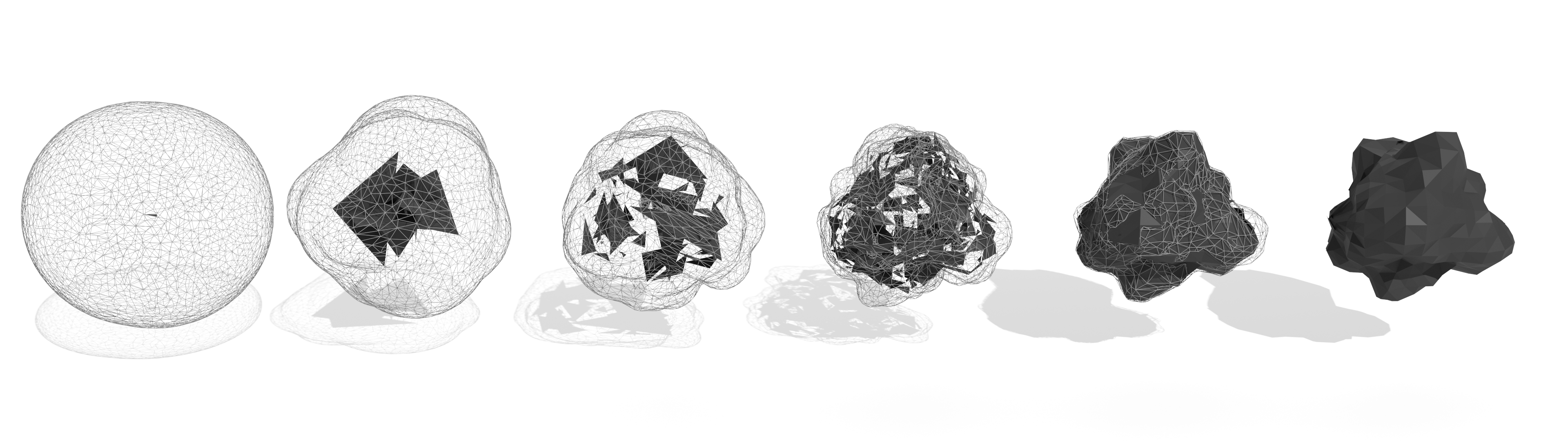
Figure 1: Surrogate triangle hierarchy for a “bumped sphere”. The actual sphere geometry $\mathbb{T}_{h}$ is shown on the right. From left to right: Finer and finer surrogate representations incl. their $\epsilon$-environments. The coarser a representation, the lower the triangle count and the larger the corresponding $\epsilon$. The surrogate triangles are weakly connected. The right most geometry is the actual particle with a closed surface.

DEM codes spend most of their runtime on collision detection [14, 16, 17, 20]. We tighten the challenge and study a DEM prototype over particles where (i) rigid particles have massively differing size, (ii) rigid particles are discretised by many triangles, and (iii) rigid particles have complicated, non-convex shapes. Our code supplements each rigid particle with an $\epsilon$-area [3, 2, 23, 25] and considers two particles to be “in contact” if their $\epsilon$-environment overlaps. This yields a weak compressibility model, where the contact points are unique up to an $\epsilon$-displacement. Yet, both the arrangement and the topology of these points still can change significantly between any two time steps, while the collision models using the contact data remain inherently stiff. Large-scale DEM codes require the comparison of many particles per time step. Efficient many-body simulations employ techniques such as neighbour lists, cell or tree meta data structures [11, 16, 2, 23] to narrow down the potential collisions, i.e. to identify particle pairs which might collide as they are spatially close. After this pre-processing or filtering step, they detect collision points between particle pairs. We focus exclusively on the particle-particle comparison challenge, as efficient algorithms for the neighbourhood identification—including techniques for challenging shapes and massively differing sizes—are known.

Our work proposes a multiscale contact detection scheme which brings down the compute time for the contact detection aggressively. We can handle complex, non-convex shapes and even speed up implicit time stepping significantly. The latter is, so far, prohibitively expensive for most codes. To reduce the runtime, our approach phrases the contact search between two particles as an iterative algorithm over multiple resolutions where coarser particle resolutions act as surrogates. This idea enables us to introduce five algorithmic optimisations: First, the surrogates help us to identify “no contact” constellations quickly. In this case, we can immediately terminate the search algorithm. The surrogates yield a generalisation of classic bounding sphere checks—if two bounding spheres do not overlap, the underlying objects can not overlap—to highly non-spherical geometries. Second, we exploit that we do not represent surrogate resolutions as a plain level of detail [1] but make them form a tree: If we identify a potential collision, only those sections of the geometry are “up-pixeled” from where a collision point might arise from. We increase the resolution locally. The complexity per iterative step thus does not grow exponentially as we switch to more accurate geometric representations. Instead we tend to have a linear increase of cost as we use finer and finer geometric models. Third, the surrogate resolutions yield conservative estimates of the force that might result from a contact point. Once we employ an implicit time stepping scheme with a Picard iteration, we can permute the iterative solver loop and the resolution switches such that the Picard iteration forms the outer loop which zaps through resolution levels upon demand. The cheap surrogates provide an educated guess to the iterative force calculation and thus accelerate the convergence. Fourth, we phrase the contact detection as a distance minimisation problem [15, 16]. The minimisation problem is solved iteratively through an additional, embedded Newton which approximates the Jacobian via a diagonal matrix and runs through a prescribed number of sweeps. Once more, we permute the loop over triangle pairs and the Picard iterations to improve the vectorisation suitability. Finally, we acknowledge that an iterative minimisation subject to a prescribed iteration count can fail if the underlying geometric problem is ill-posed. In such cases, we eventually postprocess it by falling back to a comparison-based distance calculation. However, this is only required on the finest mesh, whereas we use non-convergence within the surrogate tree as sole “refinement criterion” (use a finer mesh) that does not feed forces into the implicit time stepping.

To the best of our knowledge, our rigorous multiscale idea, which can be read as a combination of (i) loop permutation and fusion, (ii) adaptive mesh refinement, (iii) a generalisation of volume bounding hierarchies [6, 9, 10, 12, 13] and (iv) an approximate, weak closest-triangle formulation [15, 16], is unprecedented. Its reduction of computational cost plus its excellent vectorisation character in combination with the fact that rigid body simulations scale well by construction—the extremely short-range interactions fit well to domain decomposition—brings implicit DEM simulations for triangulated, non-convex shapes within practical applications into reach. The core algorithmic ideas furthermore have an impact well beyond the realm of DEM. The search for nearest neighbours, i.e. contact within a certain environment, is, for example, also a core challenge behind fluid-structure interaction (FSI).

The manuscript is organised as follows: We first introduce our algorithmic challenge and a textbook implementation of both explicit and implicit time stepping for it (Section 2). An efficient contact detection between triangulated surfaces of two particles via a minimisation problem is introduced next (Section 3), before we rewrite the underlying geometric problem as a multiresolution challenge and introduce our notion of a surrogate data structure (Section 4). In Section 5, we bring both the efficient triangle comparisons and the tree idea together as we plug them into an implicit time stepping code, before we allow the non-linear equation system solvers’ iterations to move up and down within the surrogate tree. This is the core contribution of the manuscript. Following the discussion of some numerical results (Section 6), we sketch future work and close the discussion.

2 Algorithmic framework

We study a system of $|\mathbb{P}|$ rigid bodies (particles). Each particle $p\in\mathbb{P}$ has a velocity $v(p,t)$ and an angular velocity $\omega(p,t)$ which determine its change of position and rotation. Each is described by a triangular tessellation $\mathbb{T}(p,t)$. $t\geq 0$ is the simulation time. We may assume that $\mathbb{T}(p,t)$ spans a well-defined, closed surface represented by a mesh where no two triangles intersect, and we can “run around” a particle infinitely often without falling into a gap. While the triangulation of the object is time-invariant, it moves and rotates over time and therefore depends on $t$.

Algorithm 1 High-level pseudo code for an explicit Euler for rigid particles. The continues properties $v(p,t),\omega(p,t)$ and $\mathbb{T}(p,t)$ are discretised in time and thus become $v(p),\omega(p)$ and $\mathbb{T}(p)$. $t$ is the (discretised) time, $\Delta t$ the time step size.

1:while $t<T_{\mbox{terminal}}$ do $\triangleright$ We simulate over a time span

2:   $\forall p_{i}\in\mathbb{P}:\ \mathbb{C}(p_{i})\leftarrow\emptyset$ $\triangleright$ Clear set of collisions for particle $p_{i}$

3:   for $p_{i},p_{j}\in\mathbb{P},\ p_{i}\not=p_{j}$ do $\triangleright$ Run over all particle pairs

4:     $\mathbb{C}(p_{i})\leftarrow\mathbb{C}(p_{i})\cup$ findContacts($\mathbb{T}(p_{i}),\mathbb{T}(p_{j}$))

5:     $\mathbb{C}(p_{j})\leftarrow\mathbb{C}(p_{j})\cup$ findContacts($\mathbb{T}(p_{i}),\mathbb{T}(p_{j})$)

6:   end for

7:   for $p_{i}\in\mathbb{P}$ do

8:     $\mathbb{T}(p_{i})\leftarrow$ update($\mathbb{T}(p_{i}),v(p_{i}),\omega(p_{i}),\Delta t$) $\triangleright$ Update geometry

9:   end for$\triangleright$ using velocity, rotation and time step size

10:   for $p_{i}\in\mathbb{P}$ do

11:     $(dv,d\omega)\leftarrow$ calcForces($\mathbb{C}(p_{i})$)

12:     $(v,\omega)(p_{i})\leftarrow(v,\omega)(p_{i})+\Delta t\cdot(dv,d\omega)$ $\triangleright$ Update velocity and rotation

13:   end for

14:   $t\leftarrow t+\Delta t$

15:end while

Algorithm 2 Contact identification between two particles $p_{i}$ and $p_{j}$.

1:function findContacts($\mathbb{T}(p_{i}),\mathbb{T}(p_{j})$)

2:   $\mathbb{C}=\emptyset$

3:   for $t_{i}\in\mathbb{T}(p_{i}),t_{j}\in\mathbb{T}(p_{j}),\ t_{i}\not=t_{j}$ do $\triangleright$ Run over all triangles pairs

4:     $c\leftarrow\textsc{contact}(t_{i},t_{j})$ $\triangleright$ Find closest point in-between $t_{i}$ and $t_{j}$ and compare normal

5:     if $c\not=\bot$ then $\triangleright$ $|n|$ against $\epsilon$; return $\bot$ if $|n|>\epsilon$

6:        $\mathbb{C}\leftarrow\mathbb{C}\cup\{c\}$

7:     end if

8:   end for

9:   return $\mathbb{C}$

10:end function

Time stepping

A straightforward high-level implementation of an explicit Euler for DEM consists of a time loop hosting a sequence of further loops (Algorithm 1): The first inner loop identifies all contact points between the particles. Once we know all contact points per particle, we can determine a velocity and rotation update ($dv(p)$ and $d\omega(p)$) per particle. Before we do so, we update the particles’ positions using their velocity and angular momentum. Finally, we progress in time. Euler-Cromer would result from a permutation of the update sequence.

It is impossible to simulate exact incompressibility with explicit time stepping schemes when no interpenetration is allowed: Everytime we update a particle, we run risk that it slightly penetrates another one due to the finite time step size $\Delta t$. At the same time, particles exchange no momentum as long as they are not in direct contact yet. The momentum exchange remains “trivial” until we have violated the rigid body constraint. For these two reasons, we switch to a weak incompressibility model where each particle is surrounded by an $\epsilon>0$ area [3, 25, 23, 2]. The area is spanned by the Minkovski sum of the triangles from $\mathbb{T}(p,t)$ and a sphere of radius $\epsilon$ minus the actual rigid object. Without loss of generality, we assume a uniform $\epsilon$ per particle. Our formalism is equivalent to a soft boundary formulation with an extrusive surface.

Definition 2.1 (Contact point).

Each particle is surrounded by an $\epsilon$-environment. Two particles are in contact, if their $\epsilon$-environment overlaps. Overlaps yield contact points which in turn yield forces.

We parameterise each contact point with its penetration depth: Our contact detection in Algorithm 2 identifies the closest path between two triangles. A potential contact point $c$ is located at the centre of this line. It is equipped with a normal $n(c)$, which points from the contact point towards either of the closest triangles (Figure 2). There is an overlap between the two $\epsilon$-augmented triangles if and only if $|n(c)|\leq\epsilon$, that is if the $\epsilon$-environments penetrate. In this case $c$ is added to the set of collision points.

With a set of contact points plus their normals and dimensionless masses $M(p_{i})$ and $M(p_{j})$, we can derive the force acting on a particle.

$$F(c)=\frac{n(c)}{|n(c)|}K_{s}(1-\frac{|n(c)|}{\epsilon})\sqrt{\frac{1}{\frac{1}{M(p_{i})}+\frac{1}{M(p_{j})}}}$$

computes the force arising from one contact point by mapping the $\epsilon$-area onto a simple spring with a perpendicular friction force yet without any empirical damping [8]. The force depends on the contact normal $n(c)$ and applies to both colliding particles $p_{i}$ and $p_{j}$ subject to a minus sign for one of them. It is calibrated by a spring constant $K_{s}=1,000$ . A particle’s total force is then the sum over the individual contact forces. Taking the centre of mass, the total mass and the mass distribution of a particle into account, the total force and total torque determine its acceleration and angular acceleration [5].

This is a simplistic presentation—we ignore for example sophisticated interaction functions which distinguish contact points from contact faces— where the discontinuous force that arises at a contact is approximated by a “fade-in” force as two particles approach each other: Over an interval of size $\epsilon$, the force smoothly approximates the target force, as the penetration depth $|n(c)|$ increases. The simple physics allow us to focus on the core challenge how to find contact points efficiently.

Implementation remark 1. As we work with triangulated objects and derive contact points from triangle-triangle comparisons, the algorithm identifies some contact points redundantly: If the closest distance between two objects is spanned by two object vertices $x_{i}$ and $x_{j}$, every triangle combination $t_{i}$ and $t_{j}$ where $t_{i}$ is adjacent to $x_{i}$ and $t_{j}$ to $x_{j}$ finds the same contact point and consequently adds it to $\mathbb{C}$ (Algorithm 2). The set notation for $\mathbb{C}$ highlights that we do not work with redundant contact points: In the implementation, we run over $\mathbb{C}$ and merge close-by contact points, i.e. points closer than $\epsilon$, into one average point. This filter step prior to any use of the elements from $\mathbb{C}$ is necessary, as we work with floating point arithmetics and an $\epsilon>0$, i.e. a contact point is not a unique point in space and might temporarily exist multiple times within $\mathbb{C}$ with slightly different coordinates. $\square$

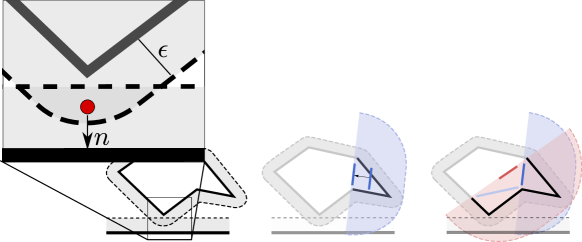
Figure 2: A pair of objects (black, solid) with their $\epsilon$-environment (black, dotted) collide. In the present sketch, one object is a “spherical” particle spanned by six edges, while the other object is a plane at the bottom. Left: Two-dimensional sketch of the contact point concept. The zoom-in shows the contact point which is located in the middle of the overlap region. The contact normal is directed from the middle point towards the closest point on one of the objects involved. Middle: When an object hosts very extruded features, we slightly shrink the surrogate such that the surrogate without $\epsilon$ becomes a closer fit around the ”un-bumped” real geometry. We trade such a surrogate for a bigger $\epsilon$. Empirical evidence suggests that this yields slightly advantageous forces within a multiscale iterative solve. Right: The conservative property of the surrogate triangles states that all fine level geometry (including its epsilon boundary) must be encompassed by the surrogate’s epsilon. This doesn’t suggest that all surrogate children are included.

Algorithm 3 High-level pseudo code for an implicit Euler.

1:while $t<T_{\mbox{terminal}}$ do $\triangleright$ We simulate over a time span

2:   $\forall p_{i}\in\mathbb{P}:\ \mathbb{T}^{\text{guess}}(p_{i})\leftarrow\mathbb{T}(p_{i}),\ v^{\text{guess}}(p_{i})\leftarrow v(p_{i}),\ \omega^{\text{guess}}(p_{i})\leftarrow\omega(p_{i})$

3:   while $\mathbb{T}^{\text{guess}},v^{\text{guess}}$ or $\omega^{\text{guess}}$ change significantly for any $p$ do

4:     $\forall p_{i}\in\mathbb{P}:\ \mathbb{C}(p_{i})\leftarrow\emptyset$ $\triangleright$ Clear set of collisions for particle $p_{i}$

5:     for $p_{i},p_{j}\in\mathbb{P},\ p_{i}\not=p_{j}$ do $\triangleright$ Run over all particle pairs

6:        $\mathbb{C}(p_{i})\leftarrow\mathbb{C}(p_{i})\cup$ findContacts($\mathbb{T}^{\text{guess}}(p_{i}),\mathbb{T}^{\text{guess}}(p_{j})$)

7:        $\mathbb{C}(p_{j})\leftarrow\mathbb{C}(p_{j})\cup$ findContacts($\mathbb{T}^{\text{guess}}(p_{i}),\mathbb{T}^{\text{guess}}(p_{j})$)

8:     end for

9:     for $p_{i}\in\mathbb{P}$ do

10:        $(dv,d\omega)\leftarrow$ calcForces($\mathbb{C}(p_{i})$)

11:        $(v^{\text{guess}},\omega^{\text{guess}})(p_{i})\leftarrow(v,\omega)(p_{i})+\Delta t\cdot(dv,d\omega)$

12:        $\mathbb{T}^{\text{guess}}(p_{i})\leftarrow$ update($\mathbb{T}(p_{i}),v^{\text{guess}}(p_{i}),\omega^{\text{guess}}(p_{i}),\Delta t$)

13:     end for

14:   end while

15:   $\forall p_{i}\in\mathbb{P}:\ \mathbb{T}(p_{i})\leftarrow\mathbb{T}^{\text{guess}}(p_{i}),\ v(p_{i})\leftarrow v^{\text{guess}}(p_{i}),\ \omega(p_{i})\leftarrow\omega^{\text{guess}}(p_{i})$

16:   $t\leftarrow t+\Delta t$

17:end while

Implicit time stepping

An implicit Euler for a DEM code has to solve a non-trivial, non-linear equation system per time step. Non-trivial means that the system’s sparsity pattern depends on the solution of the system itself. It is determined by the contact point search: we obtain entries in the interaction matrix where the corresponding normal $|n|\leq\epsilon$. Non-linearity means that the quantities in the interaction matrix (forces) depend on the (guess of the) geometries’ arrangement.

Assumption 1.

Our implicit time stepping problem exhibits a contraction property, i.e. Picard iterations can solve the underlying non-linear equation system.

As our non-linear system is “well-behaved”—we employ reasonably small $\Delta t$—we rely on a fixed-point formulation of the implicit time stepping and employ Picard iterations, i.e. we approximate the velocity and angular velocity $(dv,d\omega)(p)(t)$ through a repeated application of the contact detection plus its following force calculation (Algorithm 3). We assume that we remain within the Picard iterations’ region of convergence.

Picard avoids the assembly and inversion of an equation system. However, many contact points enter the algorithm temporarily throughout the iterations, which eventually are not identified as contacts. This happens, for example, if we rotate the particles “too far” throughout the iterations. Despite small $\Delta t$, we cannot provide an upper bound on the number of Picard iterations required or make assumptions on the (temporarily) identified contact points, i.e. the cost per iteration.

Notation and terminology

Any particle $p\in\mathbb{P}$ has a (closed) volume $V(p)$ which is spanned by its triangular surface $\mathbb{T}(p)$. Since we stick to explicit and implicit single-step, single shot methods, we omit the parameterisation $(t)$ from hereon.

$$p_{1}\cap p_{2}=\emptyset\qquad\forall p_{1},p_{2}\in\mathbb{P}\ \text{with}\ p_{1}\not=p_{2},$$

as we have rigid, non-penetrating objects. Consequently, $\mathbb{T}(p_{1})\cap\mathbb{T}(p_{2})=\emptyset$. The particles’ triangles do not intersect. Yet, as each particle is surrounded by an $\epsilon$-layer, our particles’ triangles $t\in\mathbb{T}(p)$ unfold into a set of volumetric objects $t^{\epsilon}\in\mathbb{T}^{\epsilon}(p)$, and our particles’ volumes are extended $p\subset p^{\epsilon}$, too. Overlaps between extended volumes do exist and yield contact points:

(1) $$p_{1}^{\epsilon}\cap p_{2}^{\epsilon}\not=\emptyset\ \Rightarrow\mbox{contact point}$$

which is equivalent to

$$\exists t_{1}\in\mathbb{T}(p_{1}),t_{2}\in\mathbb{T}(p_{2}):\quad t_{1}^{\epsilon}\cap t_{2}^{\epsilon}\not=\emptyset\ \Rightarrow\mbox{contact point}.$$

A contact point $c$ between two triangles $t_{i}$ and $t_{j}$ in (1) is located at

(2) $$x(c)=\frac{1}{2}(t_{1}(a_{1},b_{1})+t_{2}(a_{2},b_{2}))\ \text{with}\ \operatorname*{arg\,min}_{a_{1},b_{1},a_{2},b_{2}\in[0,1]}\frac{1}{2}\|t_{1}(a_{1},b_{1})-t_{2}(a_{2},b_{2})\|^{2},$$

if $t_{1}$ and $t_{2}$ are surrounded by the same $\epsilon$ halo. For different $\epsilon$s, the weights for $x(c)$ have to be adapted accordingly. $a_{1},b_{2}$ are Barycentric coordinates within $t_{1}$, i.e. $t_{1}(a_{1},b_{1})$ returns a position within the triangle. $a_{2}$ and $b_{2}$ are the counterparts for $t_{2}$. If $x(c)$ is the position of the contact point $c$, the corresponding normal $n(c)=t_{1}(a_{1},b_{1})-x(c)$ or $n(c)=t_{2}(a_{2},b_{2})-x(c)$.

3 Iterative contact detection via distance minimisation

To find the closest point between two triangles is a classic computational geometry problem [11]. We rely on three different algorithms to solve it:

Direct distance calculation (comparison-based)

A comparison-based identification of contact points consists of two steps. First, we compute the distance from each vertex of the two triangles to the closest point on the other triangle as well as the distance between each pair of edges between the two triangles [11]. This yields six point-to-triangle distance tests and nine edge-to-edge distance tests. In a second step, we select the minimum distance out of the 15 combinations. This brute force calculation yields an exact solution—agnostic of truncation errors—yet requires up to 30+14 comparisons (if statements) per triangle pair, which we tune via masking, blending and early termination [21]. Dealing with the cases where intersections between triangles is possible requires an additional six edge-to-plane distance tests, where intersections outside the area of the triangle are discounted.

Iterative distance calculation

As an alternative to a comparison-based approach, we replace the geometric checks with a functional where we minimise the distance between the two planes spanned by the triangles but add the admissibility conditions over the Barycentric coordinates as Lagrangian parameters [15, 16]. In line with (2), let $a,b\in[0,1]$ describe any point on their respective triangle:

(3) $$\operatorname*{arg\,min}_{a_{1},b_{1},a_{2},b_{2}}J(a_{1},b_{1},a_{2},b_{2}):= \operatorname*{arg\,min}_{a_{1},b_{1},a_{2},b_{2}}\underbrace{\frac{1}{2}\|t_{i}(a_{1},b_{1})-t_{j}(a_{2},b_{2})\|^{2}}_{=:\hat{J}(a_{1},b_{1},a_{2},b_{2})}+\alpha_{\text{iterative}}\Big{(}$$

$$\max(0,a_{1}-1)+\min(-a_{1},0)+\max(0,b_{1}-1)+$$

$$\max(-b_{1},0)+\max(0,a_{1}+b_{1}-1)+$$

$$\max(0,a_{2}-1)+\min(-a_{2},0)+\max(0,b_{2}-1)+$$

$$\max(-b_{2},0)+\max(0,a_{2}+b_{2}-1)\Big{)}.$$

This is a weak formulation of the challenge, since any $\alpha_{\text{iterative}}<\infty$ allows the closest distance line between two triangles to be rooted slightly outside the very triangles.

The minimisation problem can be solved via Newton iterations. However, the arising Hessian becomes difficult to invert or non-invertible for close-to-parallel or actually parallel triangles. We therefore regularise it by adding a diagonal matrix. After that, we approximate the regularised Hessian and update the minimisation and constraints alternatingly:

$$(a_{1},b_{1},a_{2},b_{2})^{(n+0.5)} = (a_{1},b_{1},a_{2},b_{2})^{(n)}-\text{diag}^{-1}\Big{(}\hat{H}(a_{1},b_{1},a_{2},b_{2})^{(n)}$$

$$+\alpha_{\text{regulariser}}\ id\Big{)}\nabla_{a_{1},b_{1},a_{2},b_{2}}\hat{J}(a_{1},b_{1},a_{2},b_{2})^{(n)}$$

(4) $$(a_{1},b_{1},a_{2},b_{2})^{(n+1)} = (a_{1},b_{1},a_{2},b_{2})^{(n+0.5)}-\text{diag}^{-1}\Big{(}\tilde{H}(a_{1},b_{1},a_{2},b_{2})^{(n+0.5)}$$

$$+\alpha_{\text{regulariser}}\ id\Big{)}\nabla_{a_{1},b_{1},a_{2},b_{2}}\tilde{J}(a_{1},b_{1},a_{2},b_{2})^{(n+0.5)}$$

$\alpha_{\text{regulariser}}>0$ is small, while ⁽ⁿ⁾ is the iteration index. The $\hat{J}$ and its Hessian correspond to the quadratic term of the actual functional in (3) aka (2). $\tilde{J}$ and its Hessian cover the remaining penalty terms, i.e. $J-\hat{J}$. However, we omit the Dirac terms in there, i.e. we explicitly drop terms that enter the formulae for $a_{1}=0,a_{1}=1,b_{1}=0,\ldots$. Our solver iterates back and forth between the $\hat{J}$-minimisation and a fullfillment of the constraints. This modified Newton becomes a gradient descent, where the step size is adaptively chosen by analysing an approximation of the inverse to the Hessian.

Hybrid distance calculation

If two subsequent iterates $|J(a_{1},b_{1},a_{2},b_{2})^{(n+1)}-J(a_{1},b_{1},a_{2},b_{2})^{(n)}|\leq C\epsilon$, we have found an actual minimum over functional (3) and can terminate the minimisation. In this case, we assume that $a_{1},b_{1},a_{2},b_{2}$ identify the minimum distance. Without further analysis, it is impossible to make a statement on the upper bound on $n$. Our hybrid algorithm therefore eliminates the termination criterion and imposes $n\leq N_{\texttt{iterative}}$. Consequently, it labels a distance calculation as invalid if $|J(a_{1},b_{1},a_{2},b_{2})^{(N_{\texttt{iterative}})}-J(a_{1},b_{1},a_{2},b_{2})^{(N_{\texttt{iterative}}-1)}|>C\epsilon$. The iterative code’s result realises a three-valued logic: “found a contact point”, “there is no contact”, or “has not terminated” (Algorithm 4).

Our hybrid algorithm invokes the modified iterative algorithm. If the result equals “not terminated” ($\odot$), the hybrid algorithm falls back to the comparison-based distance calculation. It is thus not really a third algorithm to find a contact point, but a combination of the iterative scheme with the comparison-based approach serving as a posteriori limiter.

Algorithm 4 A hybrid, batched reformulation of the iterative distance calculation. The iterative sweep over a whole batch of triangles is stripped of a dynamic stopping criterion (top) and therefore yields three types of results per triangle pair: $x$ holds a coordinate if the Barycentric coordinates yield a contact point, or $\bot$ if they yield no contact point, or $\odot$ if the triangle combination has to be postprocessed with the comparison-based algorithm (bottom).

1:for $t_{i}\in\mathbb{T}(p_{i}),\ t_{j}\in\mathbb{T}(p_{j}),\ t_{i}\not=t_{j}$ do

2:   $(a_{1},b_{1},a_{2},b_{2},n)(t_{i},t_{j})\leftarrow 0$ $\triangleright$ Variables per triangle pair allow us to vectorise

3:   $J_{\text{old}}(t_{i},t_{j})\leftarrow\infty$ $\triangleright$ over triangles in $\mathbb{T}$

4:   $J(t_{i},t_{j})=J(a_{1}(t_{i},t_{j}),b_{1}(t_{i},t_{j}),a_{2}(t_{i},t_{j}),b_{2}(t_{i},t_{j}))$ $\triangleright$ Functional from (3)

5:   while $n\leq N_{\text{iterative}}$ do $\triangleright$ Fixed iteration count instead of $|J-J_{\text{old}}|>C\epsilon$

6:     $J_{\text{old}}(t_{i},t_{j})\leftarrow J(t_{i},t_{j})$

7:     update $a_{1}(t),b_{1}(t),a_{2}(t),b_{2}(t)$ $\triangleright$ Modified gradient descent from (4)

8:     $J(t_{i},t_{j})=J(a_{1}(t_{i},t_{j}),b_{1}(t_{i},t_{j}),a_{2}(t_{i},t_{j}),b_{2}(t_{i},t_{j}))$

9:     $n\leftarrow n+1$

10:   end while

11:   $x(t_{i},t_{j})\leftarrow\left\{\begin{array}[]{cc}\frac{1}{2}(t_{i}(a_{1},b_{1})-t_{j}(a_{2},b_{2}))(t_{i},t_{j})&\text{if}\ |J(t_{i},t_{j})-J_{\text{old}}(t_{i},t_{j})|\leq C\epsilon\wedge\hat{J}(t_{i},t_{j})\leq 2\epsilon^{2}\\ \bot&\text{if}\ |J(t_{i},t_{j})-J_{\text{old}}(t_{i},t_{j})|\leq C\epsilon\wedge\hat{J}(t_{i},t_{j})>2\epsilon^{2}\\ \odot&\text{otherwise}\end{array}\right.$

12:end for

13:

14:for $t_{i}\in\mathbb{T}(p_{i}),\ t_{j}\in\mathbb{T}(p_{j}),\ t_{i}\not=t_{j}$ do

15:   if $x(t_{i},t_{j})=\odot$ then

16:     $\hat{n}(t_{i},t_{j})\leftarrow$ shortest distance vector between $t_{i}$ and $t_{j}$ $\triangleright$ Use comparison-based algorithm

17:     $\hat{x}(t_{i},t_{j})\leftarrow$ is central point on line identified by $\hat{n}(t_{i},t_{j})$

18:     $x(t_{i},t_{j})\leftarrow\left\{\begin{array}[]{cc}\hat{x}(t_{i},t_{j})&\text{if}\ |\hat{n}(t_{i},t_{j})|\leq 2\epsilon\\ \bot&\text{otherwise}\end{array}\right.$ $\triangleright$ Eliminate $\odot$ entries in result

19:   end if

20:end for

Implementation remark 2. Triangle meshes are typically held as graphs over vertex sets. We flatten this graph prior to the contact detection: A sequence of $|\mathbb{T}|$ triangles is converted into a sequence of $3\cdot 3\cdot|\mathbb{T}|$ floating point values, i.e. each triangle is represented by the coordinates (three components) of its three vertices. Such a flat data structure can be generated once prior to the first contact detection. All topology is lost in this representation and vertex data is replicated—it is a triangle soup—but the data is well-suited to be streamed without indirect memory lookups. Per update of the position and rotation, every coordinate is subject to an affine transformation.

$\square$

4 A multiresolution model

The cost to compare two particles $p_{i}$ and $p_{j}$ is determined by their triangle counts $|\mathbb{T}(p_{j})|$ and $|\mathbb{T}(p_{j})|$. To reduce this cardinality, we construct geometric cascades of triangle models per particle—the surrogate models (Fig. 1)—and plug representations from this cascade into Algorithm 2.

Definition 4.1.

A surrogate model $\mathbb{T}_{k}(p),\ k\geq 1$ is a triangle-based geometric approximation of a particle described by $\mathbb{T}(p)$. A sequence of surrogate models $\{\mathbb{T}_{1}(p),\mathbb{T}_{2}(p),\mathbb{T}_{3}(p),\ldots\}$ for $p$ with its volumetric extensions $\mathbb{T}_{k}^{\epsilon}(p)$ hosts efficient (Definition 4.2), conservative (Definition 4.3), and weakly connected (Definition 4.5) abstractions of $\mathbb{T}(p)$.

Surrogate models are different representations of a particle. The term “cascade” highlights that each particle is assigned a whole sequence of representations. These representations can step in for our real geometry and are a special class of bounding volume techniques [11]. To simplify our notation, $\mathbb{T}_{0}(p):=\mathbb{T}(p)$, i.e. the $k=0$ surrogate model is the geometric object itself. The bigger $k$, the coarser, i.e. more abstract the surrogate. . Furthermore, we emphasise that the $\epsilon$ is a generic symbol, i.e. each surrogate model hosts its own, bespoke $\epsilon$-environment.

Definition 4.2.

A surrogate model $\mathbb{T}^{\epsilon}_{k_{i}}(p_{i})$ is efficient if, for any other model $\mathbb{T}^{\epsilon}_{k_{j}}(p_{j})$, finding all contact points between $\mathbb{T}^{\epsilon}_{k_{i}}(p_{i})$ and $\mathbb{T}^{\epsilon}_{k_{j}}(p_{j})$ is cheaper than finding all contact points between $\mathbb{T}^{\epsilon}_{\hat{k}_{i}}(p_{i})$ and $\mathbb{T}^{\epsilon}_{k_{j}}(p_{j})$ for all $0\leq\hat{k}_{i}<k_{i}$.

We assume an almost homogeneous cost per triangle-to-triangle comparison—an assumption that is shaky for the hybrid comparison and subject to vectorisation efficiency and memory management effects. Hence, the triangle count of surrogate models decreases with increasing $k$, i.e. $|\mathbb{T}_{k}|\ll|\mathbb{T}_{k+1}|$.

Definition 4.3.

A surrogate model $\mathbb{T}_{k_{i}}(p_{i})$ inducing $\mathbb{T}_{k_{i}}^{\epsilon}(p_{i})$ is conservative if

$$\forall p_{i},p_{j},k_{i},k_{j}:\ \mathbb{T}_{k_{i}}^{\epsilon}(p_{i})\cap\mathbb{T}_{k_{j}}^{\epsilon}(p_{j})=\emptyset\ \Rightarrow\ \mathbb{T}^{\epsilon}(p_{i})\cap\mathbb{T}^{\epsilon}(p_{j})=\emptyset.$$

Conservative means that any two surrogates of two particles are in contact (overlap) if the two particles are in contact. Yet, this does not have to hold the other way round: If their surrogates are in contact, there might still be gaps between the particles, i.e. there might be no contact point.

Corollary 4.4.

Let a surrogate model hierarchy $\mathbb{T}_{k}(p),\ k\geq 1$ be monotonous if

$$\forall 1\leq\hat{k}<k:\quad\forall t_{\hat{k}}^{\epsilon}\in\mathbb{T}_{\hat{k}}^{\epsilon}(p):\quad t_{\hat{k}}^{\epsilon_{\hat{k}}}\subseteq\bigcup_{t\in\mathbb{T}_{k}^{\epsilon}(p)}t.$$

Our surrogate hierarchies do not have to be monotonous.

A monotonous cascade of triangles plus $\epsilon$-environments would grow in space as we move up the hierarchy of models. Therefore, we do not impose it, even though monotonicity would imply conservativeness “for free”. Empirical evidence suggests that abandoning monotonicity allows us to work with significantly tighter $\epsilon$-choices per level. Yet, it also implies that we generally cannot show algorithm correctness through plain induction.

Classic level-of-detail algorithms require a coarsened representation of a triangulated model to preserve certain properties such as connected triangle surfaces or the preservation of certain features such as sharp edges. Our surrogate models however are to be used as temporary replacements within our calculations. We thus can ask for weak representations of the geometries:

Definition 4.5.

The triangles of a particle have to span a connected surface. For surrogate models, there is no such constraint. Therefore, the surrogate models can be weakly connected: Their triangles can be disjoint with gaps in-between or they can intersect each other. A surrogate’s $\epsilon$-environment is connected however, and it covers (overlaps) all connectivity of the original model.

The connectivity addendum in Definition 4.5 motivates the term weakly connected. It clarifies that we—despite the disjoint, anarchic configuration of a surrogate triangle set (Figure 1)— cannot miss out on some geometry extrema such as sharp edges due to tests with surrogates: If there is no contact between two surrogates, there is also no contact between their real discretisations.

Definition 4.3 implies that we can use surrogate models as guards and run through them for coarse to fine: If there are no contact points between two surrogate models, there can be no contact points for the more detailed models. We can stop searching for contact points immediately. It does however not hold the other way round. Definition 4.2 implies immediately that the number of triangles that we examine in such an iterative approach is monotonously growing. Definition 4.5 gives us the freedom to construct such triangle hierarchies, as it strips us from many geometric constraints.

Definition 4.6.

Let $\mathcal{T}$ be a directed acycling graph where each node represents a set of triangles. The level $\ell$ of a node is its distance (edge count) from the root node in $\mathcal{T}$. The resulting graph is a surrogate tree if and only if

1. the root node hosts the coarsest surrogate model $\mathbb{T}_{k_{\text{max}}}$;

2. the union over all leaf sets yields the particle triangulation $\mathbb{T}_{0}$;

3. any triangle is a surrogate for the union over its children’s triangle sets.

With Definition 4.6, the union over all sets with the same level yields the surrogate model $\mathbb{T}_{k_{\text{max}}-\ell}$. We use $N_{\text{surrogate}}$ to denote the number of children of a surrogate triangle. $N_{\text{surrogate}}$ does not have to be uniform over the tree, i.e. is a generic symbol. If we have a surrogate model, take the nodes within the tree which hold its triangles, and replace the triangles with those triangles stored within children nodes, we obtain the next finer surrogate. A surrogate tree is a generalisation of the concept of a cascade of surrogates: The tree formalism allows us also to construct different, hybrid-level surrogate models if we only replace some triangles of a model with their children.

Implementation remark 3. There are multiple ways to construct surrogate trees. We construct our trees through a recursive algorithm. It starts from the triangle set $\mathbb{T}=\mathbb{T}_{0}$ of the particle and splits this set into $N_{\text{surrogate}}$ subsets of roughly the same size hosting close-by triangles. Per subset, we construct one surrogate and thus obtain a tree of depth one where the root node hosts $|N_{\text{surrogate}}|$ triangles. As long as a node within the tree hosts more triangles than a prescribed threshold, we apply the splitting recursively and thus disentangle the triangle sets further and further: Existing tree levels are pushed down or sieved through the tree hierarchy (Appendix B). A follow-up bottom-up traversal of the tree constructs well-suited surrogate triangles with appropriate $\epsilon$ choices. As we only require weakly connected surrogates, the steps within this bottom-up traversal are independent of operations on sibling nodes within the tree and can be mapped onto local minimisation problems (Appendix A). $\square$

5 Multiresolution contact detection

With our surrogate tree definition, we are in the position to propose a multiscale algorithm for an explicit Euler which utilises the tree as early stopping criterion for the search for contacts. The observations for the explicit time stepping then allow us to derive two implicit time stepping algorithms that exploit the multiscale nature of the geometry to terminate searches early and to supplement the underlying iterative algorithm with educated guesses:

5.1 Explicit Euler

Our explicit Euler exploits the multiscale hierarchy by looping over the the resolutions held in $\mathcal{T}$ top down. The tree is unfolded depth-first, and we implement an early stopping criterion: If a surrogate triangle and a triangle set from another particle do not collide, the children of the surrogate triangle in our triangle tree cannot collide either. The depth-first traversal along this branch of the tree thus can terminate early. The surrogate model unfolds adaptively.

Algorithm 5 Multiresolution contact detection within explicit time stepping. It compares two particles $p_{i}$ and $p_{j}$ given by their surrogate trees $\mathcal{T}(p_{i})$ and $\mathcal{T}(p_{j})$ with each other.

1:$\mathbb{A}_{i}\leftarrow root(\mathcal{T}(p_{i}))$, $\mathbb{A}_{j}\leftarrow root(\mathcal{T}(p_{j}))$ $\triangleright$ Set of active triangles to check

2:while $\mathbb{A}_{i}\not=\emptyset\vee\mathbb{A}_{j}\not=\emptyset$ do

3:   $\mathbb{A}_{i,\text{new}}\leftarrow\emptyset$, $\mathbb{A}_{j,\text{new}}\leftarrow\emptyset$

4:   for $t_{i}\in\mathbb{A}_{i},t_{j}\in\mathbb{A}_{j}$ do

5:     $c\leftarrow\textsc{contact\_iterative}(t_{i},t_{j})$ $\triangleright$ Use context-specific $\epsilon$ depending on $t_{i},t_{j}$

6:     if $c=\odot\wedge t_{i}\in\mathbb{T}^{\epsilon}_{0}(p_{i})\wedge t_{j}\in\mathbb{T}^{\epsilon}_{0}(p_{j})$ then $\triangleright$ Not converged on non-surrogate triangles

7:        $c\leftarrow\textsc{contact\_comparison}(t_{i},t_{j})$ $\triangleright$ Use comparison-based algorithm this time

8:     end if

9:     if $c\not=\bot$ then

10:        if $t_{i}\in\mathbb{T}^{\epsilon}_{0}(p_{i})\wedge t_{j}\in\mathbb{T}^{\epsilon}_{0}(p_{j})$ then $\triangleright$ No surrogate triangles,

11:          $\mathbb{C}(p_{i})\leftarrow\mathbb{C}(p_{i})\cup\{c\}$, $\mathbb{C}(p_{j})\leftarrow\mathbb{C}(p_{j})\cup\{c\}$ $\triangleright$ i.e. proper contact point

12:        else$\triangleright$ Unfold

13:          if $t_{i}\in\mathbb{T}^{\epsilon}_{0}(p_{i})$ then

14:            $\mathbb{A}_{i,\text{new}}\leftarrow\mathbb{A}_{i,\text{new}}\cup\{t_{i}\}$

15:          else

16:            $\mathbb{A}_{i,\text{new}}\leftarrow\mathbb{A}_{i,\text{new}}\cup\{\hat{t}:\hat{t}\sqsubseteq_{\text{child}}t_{i}\}$

17:          end if

18:          if $t_{j}\in\mathbb{T}^{\epsilon}_{0}(p_{j})$ then

19:            $\mathbb{A}_{j,\text{new}}\leftarrow\mathbb{A}_{j,\text{new}}\cup\{t_{j}\}$

20:          else

21:            $\mathbb{A}_{j,\text{new}}\leftarrow\mathbb{A}_{j,\text{new}}\cup\{\hat{t}:\hat{t}\sqsubseteq_{\text{child}}t_{j}\}$

22:          end if

23:        end if

24:     end if

25:   end for

26:   $\mathbb{A}_{i}\leftarrow\mathbb{A}_{i,\text{new}}$, $\mathbb{A}_{j}\leftarrow\mathbb{A}_{j,\text{new}}$

27:end while

The concept defines a marker (Algorithm 5): Let $\mathbb{A}$ identify a set of active nodes from $\mathcal{T}$. The union of all sets labelled by $\mathbb{A}$ yields all triangles from a particle that participate in collision checks. At the begin of a particle-to-particle comparison, only the particles’ roots are active. From there, we work our way down into finer and finer geometric representations as long as the surrogate models suggest that there might be some contacts, until we eventually identify real contact points stemming from the finest mesh.

Lemma 5.1.

The hierarchical algorithm yields exactly the same outcome as our baseline code over sets $\mathbb{T}^{\epsilon}(p_{i})$ and $\mathbb{T}^{\epsilon}(p_{j})$. Algorithm 5 is correct.

Proof 5.2.

The argument relies on three properties:

1. If a contact point is identified for a surrogate triangle, it is not added to the set of contact points. Therefore, a given active set never identifies artificial/too many contact points.

2. A contact point is added if it stems from the comparison of two triangles from the fine grid tessellations which are in the active sets.

3. Let two triangles $t_{i}^{\epsilon}$ and $t_{j}^{\epsilon}$ yield a contact point. As surrogates are conservative, they belong to nodes (triangle sets) $\mathbb{T}(p_{i})$ and $\mathbb{T}(p_{j})$ with $\mathbb{T}(p_{i})\sqsubseteq_{\text{child}}\hat{t}_{i}$ and $\mathbb{T}(p_{j})\sqsubseteq_{\text{child}}\hat{t}_{j}$ in $\mathcal{T}(p_{i})$ or $\mathcal{T}(p_{j})$, respectively. These surrogates fulfil

   $$t_{i}^{\epsilon}\cap t_{j}^{\epsilon}\not=\emptyset\Rightarrow\hat{t}_{i}^{\epsilon}\cap\hat{t}_{j}^{\epsilon}\not=\emptyset.$$

   and therefore are replaced in the active set by their children in Algorithm 1 before the respective algorithm terminates.

The correctness of the algorithm follows from bottom-up induction over the levels of $\mathcal{T}$: The property holds directly for the finest surrogate levels $\mathbb{T}_{1}$ of the tree. Any violation thus has to arise from $\mathbb{T}_{k},k\geq 2$ in $p_{i}$ or $p_{j}$. We apply the arguments recursively.

We have two triangle-to-triangle comparison strategies on the table (hybrid and comparison-based) which are robust, i.e. always yield the correct solution. If we employ the comparison-based approach only, the $c=\odot$ condition never holds and the corresponding branch is never executed. Otherwise, our algorithmic blueprint implements the hybrid’s fall-back as it automatically re-evaluates the contact search for $c=\odot$. However, it is indeed sufficient to rerun this a posteriori contact search if and only if both triangles stem from the finest triangle discretisation:

Corollary 5.3.

On the surrogate levels within the tree, it is sufficient to use the (efficient) iterative collision detection algorithm (Algorithm 4, bottom), without falling back to the comparison-based variant.

Proof 5.4.

Let $\mathbb{T}^{\epsilon}(p_{i})\cap\mathbb{T}^{\epsilon}(p_{j})\not=\emptyset$, i.e. two particles collide. We assume the lemma is wrong, i.e. the tree unfolding terminates prematurely. This assumption formally means

$$\exists t_{i}\in\mathcal{T}(p_{i}),t_{j}\in\mathcal{T}(p_{j}):r(p_{i},p_{j})=\bot,$$

with

$$\exists t_{0,i}\in\mathbb{T}(p_{i}),t_{0,j}\in\mathbb{T}(p_{j}):\ t_{0,i}\sqsubseteq_{\text{child}}\ldots\sqsubseteq_{\text{child}}t_{i}\wedge t_{0,j}\sqsubseteq_{\text{child}}\ldots\sqsubseteq_{\text{child}}t_{j}\wedge t_{i}^{\epsilon}\cap t_{j}^{\epsilon}\not=\emptyset.$$

This assumption is a direct violation of the definition of a surrogate model which has to be conservative.

5.2 Implicit Euler with multiresolution acceleration

Picard iterations can exploit the multiscale hierarchy by looping over the hierarchy levels top down: Per iteration of Algorithm 3, we have to identify all contact points for the current particle configuration. This search for contact points is the same search as we use it in an explicit Euler. If we replace the contact detection within the inner loop with our multiscale contact detection from Section 5.1, we obtain an implicit Euler where the surrogate concept is used within the Picard loop as multiresolution acceleration. The surrogate concept enters the algorithm’s implementation as a black-box.

Corollary 5.5.

An implicit Euler using surrogates within the Picard loop body to speed up the search for contact points yields the same output as a flat implicit code with the same number of Picard iterations.

Proof 5.6.

This is a direct consequence of Lemma 5.1 and implies the algorithm’s correctness.

Though we end up with exactly the same number of Picard iterations, the individual iterations are accelerated by the multiresolution technique: For a localised contact between two particles, the surrogate tree is unfolded along a single or few branches of the tree. If the nodes within the tree hold roughly the same number of triangles, the number of triangles to be compared grows linearly with the number of Picard steps. We benefit both from a zapping through the resolution levels and the localisation of contacts, i.e. the fact that two particles usually collide only in a small area compared to the overall geometric object.

5.3 Implicit multi-resolution Euler

A more bespoke implicit multiresolution algorithm arises from ideas inspired by multilevel non-linear equation system solvers. The multiscale Algorithm 5.2 consists of two nested while loops—the outer loop stems from the Picard iterations, the inner loop realises the tree unfolding—which we can permute. We obtain an algorithm that runs top-down via the active sets through the surrogate hierarchies and unfolds the trees step by step. Per unfolding step, it uses the Picard loop to converge on the selected hierarchy level. The rationale behind such a permutation is the observation that the efficiency of a nonlinear equation system solver hinges on the availability of a good initial guess. Surrogate resolution levels might be well-suited to deliver a good initial guess of what $\mathbb{T}$ looks like in the next time step. This train of thought is similar to the extension of multigrid into full multigrid. The same multigrid analogy suggests that we do not have to converge on a surrogate level, as the level supplements only a guess anyway. In the extreme case, it is thus sufficient to run one Picard iteration per unfolding step only.

Algorithm 6 Implicit time stepping algorithm where the Picard and multiresolution loop are intermingled.

1:$\forall p_{j}\not=p_{i}\in\mathbb{P}:\$ $\mathbb{A}(p_{i},p_{j})\leftarrow root(\mathcal{T}(p_{i}))$ $\triangleright$ Active sets are now parameterised over interactions

2:while $\mathbb{T}^{\text{guess}}(p_{i}),v^{\text{guess}}(p_{i}),\omega^{\text{guess}}(p_{i})$ or any $\mathbb{A}$ change significantly for any $p_{i}$ do

3:   $\forall p_{j}\not=p_{i}\in\mathbb{P}:\$ $\mathbb{A}_{\text{new}}(p_{i},p_{j})\leftarrow\emptyset$, $\mathbb{A}_{\text{new}}(p_{j},p_{i})\leftarrow\emptyset$, $\mathbb{C}(p_{i},p_{j})=\emptyset$, $\mathbb{C}(p_{j},p_{i})=\emptyset$

4:   for $p_{j}\not=p_{i}\in\mathbb{P}$ do

5:     for $t_{i}\in\mathbb{A}(p_{i},p_{j}),t_{j}\in\mathbb{A}(p_{j},p_{i})$ do

6:        $c\leftarrow\textsc{contactIterative}(t_{i},t_{j})$ $\triangleright$ Use context-specific $\epsilon$ depending on $t_{i},t_{j}$

7:        if $c=\odot\wedge t_{i}\in\mathbb{T}^{\epsilon}_{0}(p_{i})\wedge t_{j}\in\mathbb{T}^{\epsilon}_{h}(p_{j})$ then $\triangleright$ Not converged on non-surrogate triangles

8:          $c\leftarrow\textsc{contactComparisonBased}(t_{i},t_{j})$ $\triangleright$ Use comparison-based algorithm this time

9:        end if

10:        if $c\not=\bot\wedge c\not=\odot$ then $\triangleright$ Implicit guess

11:          $\mathbb{C}(p_{i})\leftarrow\mathbb{C}(p_{i})\cup\{c\}$, $\mathbb{C}(p_{j})\leftarrow\mathbb{C}(p_{j})\cup\{c\}$

12:        end if

13:        if $c=\bot$ then $\triangleright$ Add only parents

14:          $\mathbb{A}_{\text{new}}(p_{i},p_{j})\leftarrow\mathbb{A}_{\text{new}}(p_{i},p_{j})\cup\{\hat{t}:t_{i}\sqsubseteq_{\text{child}}\hat{t}\}$

15:          $\mathbb{A}_{\text{new}}(p_{j},p_{i})\leftarrow\mathbb{A}_{\text{new}}(p_{j},p_{i})\cup\{\hat{t}:t_{j}\sqsubseteq_{\text{child}}\hat{t}\}$

16:        else$\triangleright$ Widen active sets

17:          …$\triangleright$ Compare to Algorithm 5

18:        end if

19:     end for

20:   end for

21:   $\forall p_{j}\not=p_{i}\in\mathbb{P}:\$ $\mathbb{A}(p_{i},p_{j})\leftarrow\mathbb{A}_{\text{new}}(p_{i},p_{j})$, $\mathbb{A}(p_{j},p_{i})\leftarrow\mathbb{A}_{\text{new}}(p_{j},p_{i})$

22:   for $p_{i}\in\mathbb{P}$ do

23:     $(dv,d\omega)\leftarrow$ calcForces($\mathbb{C}(p_{i})$) $\triangleright$ Remove redundant contact points first

24:     $(v^{\text{guess}},\omega^{\text{guess}})(p_{i})\leftarrow(v,\omega)(p_{i})+\Delta t\cdot(dv,d\omega)$ $\triangleright$ Additional damping might be required

25:     $\mathbb{T}^{\text{guess}}(p_{i})\leftarrow$ update($\mathbb{T}(p_{i}),v^{\text{guess}}(p_{i}),\omega^{\text{guess}}(p_{i}),\Delta t$)

26:   end for

27:   for $p_{j}\not=p_{i}\in\mathbb{P}$ do $\triangleright$ Clean-up, i.e. add siblings

28:     $\triangleright$ Obsolete if surrogate nodes host only one triangle

29:     $\forall t,\hat{t}\in\mathbb{A}(p_{i},p_{j})\ \text{with}\ t\sqsubseteq_{\text{child}}\hat{t}:$ $\mathbb{A}(p_{i},p_{j})\leftarrow\mathbb{A}(p_{i},p_{j})\cup\{t^{\prime}\in\mathcal{T}(p_{i}):t^{\prime}\sqsubseteq_{\text{child}}\hat{t}\}$

30:     $\forall t,\hat{t}\in\mathbb{A}(p_{j},p_{i})\ \text{with}\ t\sqsubseteq_{\text{child}}\hat{t}:$ $\mathbb{A}(p_{j},p_{i})\leftarrow\mathbb{A}(p_{j},p_{i})\cup\{t^{\prime}\in\mathcal{T}(p_{j}):t^{\prime}\sqsubseteq_{\text{child}}\hat{t}\}$

31:     $\triangleright$ and remove “redundant” parents

32:     $\forall t\in\mathbb{A}(p_{i},p_{j}):\ \mathbb{A}(p_{i},p_{j})\leftarrow\mathbb{A}(p_{i},p_{j})\setminus\{\hat{t}\in\mathcal{T}(p_{i}):t\sqsubseteq_{\text{child}}\hat{t}\}$

33:     $\forall t\in\mathbb{A}(p_{j},p_{i}):\ \mathbb{A}(p_{j},p_{i})\leftarrow\mathbb{A}(p_{j},p_{i})\setminus\{\hat{t}\in\mathcal{T}(p_{j}):t\sqsubseteq_{\text{child}}\hat{t}\}$

34:   end for

35:end while

36:$\forall p_{i}\in\mathbb{P}:\ \mathbb{T}(p_{i})\leftarrow\mathbb{T}^{\text{guess}}(p_{i}),\ v(p_{i})\leftarrow v^{\text{guess}}(p_{i}),\ \omega(p_{i})\leftarrow\omega^{\text{guess}}(p_{i})$

37:$t\leftarrow t+\Delta t$

Our advanced variant of the implicit Euler is an outer-loop multi-resolution Picard scheme. Let the Picard loop start from the coarsest surrogate representation per particle (Algorithm 6). These representations form our initial active sets. After the Picard step, any surrogate triangle for which the hybrid algorithm has not terminated or for which we identified a contact point is replaced by its next finer representation.. In the tradition of value-range analysis, we widen the active set [4]. The Picard loop terminates if the plain algorithm’s termination criteria hold, i.e. the outcome of two subsequent iterations does not change dramatically anymore, and no surrogate tree node has unfolded anymore throughout the previous iterate.

The algorithm is completed by a clean up which removes “obsolete” triangles from the active set: If all children of a surrogate triangle do certainly not contribute a contact point anymore, they are replaced with their parent surrogate triangle. We narrow the active set.

Implementation remark 4. Different to the explicit scheme, we maintain an active set $\mathbb{A}(p_{i},p_{j})$ per particle-particle combination $p_{i},p_{j}$: A particle $p_{i}$ can exhibit a very coarse surrogate representation against one particle, while using a very detailed mesh when we compare it to another one. While the number of particle-particle combinations is potentially huge, it is small in practice, as particles are rigid and thus cannot cluster arbitrarily dense. $\square$

Our genuine multiscale formulation stresses the convergence assumptions:: While Assumption 1 guarantees the convergence of the Picard iterations on the finest level, our multi-resolution approach may push the solution into the wrong direction via the surrogate levels and thus make the initial guess on the next finer level leave the single level’s convergence domain.

Assumption 2.

We assume that a Picard iteration on any level of the surrogate trees yields a new solution on the same or a finer resolution which preserves the Picard iteration’s contraction property.

Lemma 5.7.

If Assumption 2 holds and if Algorithm 6 terminates, it delivers the correct solution.

Proof 5.8.

We have to study two cases over the active sets $\mathbb{A}(p_{i},p_{j})$ and $\mathbb{A}(p_{j},p_{i})$. First, assume that $(t_{\mathbb{A}(p_{i},p_{j})},t_{\mathbb{A}(p_{j},p_{i})})\in\mathbb{A}(p_{i},p_{j})\times\mathbb{A}(p_{j},p_{i})$ yields an invalid contact point, i.e. a contact point that does not exist in $\mathbb{T}_{0}(p_{i})$ compared to $\mathbb{T}_{0}(p_{j})$. One of the triangles has to be a surrogate triangle. They are replaced by their children and the algorithm has not terminated. Instead, we approach the solution further.

In the other case, assume that the algorithm has terminated yet misses a triangle pair $(t(p_{i}),t(p_{j}))\not\in\mathbb{T}(p_{i})\times\mathbb{T}(p_{j})$ which contributes a contact point in the plain model. Due to Definition 4.3 over conservative surrogates,

(5) $$\forall t(p_{i})\in\mathbb{T}_{0}(p_{j}),\exists\hat{t}_{\mathbb{A}(p_{i},p_{j})}\in\mathbb{A}(p_{i}):\quad t(p_{i})\sqsubseteq_{\text{child}}\ldots\sqsubseteq_{\text{child}}\hat{t}_{\mathbb{A}(p_{i},p_{j})}$$

such that $\hat{t}_{\mathbb{A}(p_{i},p_{j})}$ yields a contact point. This point is eventually removed as the corresponding $\hat{t}_{\mathbb{A}(p_{i},p_{j})}$ is replaced by its children. The algorithm has not terminated yet.

Lemma 5.9.

Corollary 5.10.

The removal of triangles from the active set can cause Algorithm 6 to violate Assumption 2.

Proof 5.11.

If no triangles are ever removed from the active set, the proof of Lemma 5.7 trivially demonstrates that the algorithm terminates always, as the surrogate tree is of finite depth and width. Even if we overshoot with the Picard iterations, i.e. if we violate the contraction property, we will, in the worst case, get $\mathbb{A}(p_{i},p_{j})=\mathbb{T}(p_{i})$. From hereon, the algorithm converges.

If we however remove triangles, it is easy to see that we cannot guarantee that we do not introduce cycles or even amplify oscillations. The contraction property is violated.

Proof 5.12.

Implementation remark 5. In practice, Corollary 5.10 implies that we, on the one hand, have to damp the Picard iterations. We artificially reduce the force contributions from coarse surrogate levels to avoid oscillations. On the other hand, we work with a memory set $\mathbb{U}(p_{i},p_{j})$ in which we hold references to triangles which have been removed from the active set. Once they are re-added, we veto any subsequent removal from hereon and, hence, the activation of such triangles’ surrogates. $\square$

5.4 Implementation

There are two reasons why our multi-resolution algorithms are expected to yield better performance than a straightforward textbook implementation: First and foremost, we expect the number of triangle-to-triangle comparisons to go down compared to a flat, single-level approach. The multiscale algorithm iteratively narrows down the region of a particle where contacts may arise from. These savings on the finer geometric resolutions compensate for additional checks with surrogate triangles. However, any cost amortisation has to be studied carefully—in particular for the implicit, non-linear case where trees unfold and collapse again—and it hinges upon an efficient realisation: In this context, we expect the streaming, comparison-free variants of our algorithm to benefit from vector architectures.

The multiresolution representation of an object can be computed at simulation startup as a preprocessing step. Though we keep the multiresolution hierarchy when particles move and rotate, the flattening of the active sets of triangles from $\mathcal{T}(p)$ into a sequence of coordinates is done on-the-fly and the flattened data is not held persistently.

On the one hand, this ensures that the memory overhead remains under control. On the other hand, it pays tribute to the fact that the active set changes permanently. To remain fast despite permanently changing active sets, we pick $N_{\text{surrogate}}$ such that the finest nodes within $|\mathbb{T}|$ hold triangle sequences for which streaming instructions such as AVX already pay off. The tree clusters $\mathbb{T}$ into segments that fit to the architecture, and Algorithm 4 hence does not process all triangles from $\mathbb{T}$ in one batch. Instead it runs over subchunks of batches.

We apply this argument recursively and make each non-leaf node within $\mathcal{T}$ hold a set of triangles, too. We make the nodes in the surrogate tree host many triangles and the tree overall shallow, such that the per-node data cardinality again ensures that we benefit from vector units. This “tweak $N_{\text{surrogate}}$” idea however does not fit perfectly to multiscale algorithms where the coarser tree levels typically do not occupy a complete vector length. It would be a coincidence if $|\mathbb{T}|$ and $N_{\text{surrogate}}$ yielded only nodes that fill a vector unit completely on each and every surrogate level. Therefore, we do not run triangle-to-triangle comparisions within the tree directly. Instead, we make the tree/triangle traversal collect all comparisons to be made with a buffer. Once we have identified all triangle collisions to be computed, we stream the whole buffer through the vector units. We merge the triangle representations on-the-fly.

Implementation remark 6. If our surrogate tree hosts more than one triangle per non-leaf node, the algorithm has to be completed by a further clean-up step which ensures that the active set remains consistent with the tree: It runs through the active set of a particle-particle combination once again. If any of a surrogate triangle’s children is part of the active set, the surrogate is removed from the set, but all of its children become active. Without such an additional sweep over the active set, all triangles of a node could be active plus the children of one triangle which implies that we test against the children triangle set plus their surrogate triangle. Restricting the node triangle cardinality for surrogate levels to one renders the additional clean-up unneccessary. $\square$

6 Runtime results

Our algorithms yield correct results (Lemma 5.1, Corollary 5.5 and Lemma 5.7), but they do not provide an efficiency guarantee. We hence collect runtime results, i.e. gather empirical evidence. Real-world experiments benchmarked against measurements remain out-of-scope for the present paper. We furthermore continue to focus on the actual collision detection and neglect the impact of different time step sizes—in particular comparisions between implicit and explicit schemes facilitating different stable time step choices—the cost of a coarse-grain neighbour search via a grid, e.g., and notably the construction cost for the surrogates which are done offline prior to the simulation run. All experiments are run on Intel Xeon E5-2650V4 (Broadwell) chips in a two socket configuration with $2\times 12$ cores. They run at 2.4 GHz, though TurboBoost can increase this up to 2.9 GHz. However, a core executing AVX(2) instructions will fall back to a reduced frequency (minimal 1.8 GHz) to stay within the TDP limits [7].

Our node has access to 64 GB TruDDR4 memory, which is connected via a hierarchy of three inclusive caches. They host $12\times(32+32)$ KiB, $12\times 256$ KiB or $12\times 2.5$ MiB, respectively. We obtain around 109 GB/s in the Stream TRIAD [19] benchmark on the node which translates into 4,556 MB/s per core. The node has a theoretical single precision peak performance between $2.4$ (non-AVX mode and baseline speed) and $46.4$ Gflop/s per core (AVX 2.0 FMA3 with full turbo boost). All of our calculations are ran in single precision. They are translated with the Intel 19 update 2 compiler and use the flags -std=c++17 -O3 -qopenmp -march=native -fp-model fast=2, i.e. we tailor them to the particular instruction set.

All presented performance counter data are read out through LIKWID [22]. DEM codes are relatively straightforward to parallelise as their particle-particle interaction is strongly localised: We can combine grid-based parallelism (neighbour cells) with an additional parallelisation over the particle pairs [16]. The load balancing of these concurrency dimensions however remains challenging. As our ideas reduce the comparison cost algorithmically yet do not alter the concurrency character, we stick (logically) to single core experiments to avoid biased measurements due to parallelisation or load balancing overheads. Yet, we artificially scale up the setup by replicating the computations per node over multiple OpenMP threads whenever we present real runtime data or machine characteristics, and then break down the data again into cost per replica per core. This avoids that simple problems fit into a particular cache or that memory-bound applications have exclusive access to two memory controllers.

6.1 Experimental setup

We work with two simple benchmark setups, before we validate our results for large numbers of particles. In the particle-particle setup, we study two spherical objects which are set on direct collision trajectory. They bump into each other, and then separate again. The setup yields three computational phases: While the particles approach, there is no collision and no forces act on the particles as we neglect gravity. When they are close enough, the particles exchange forces and the system becomes very stiff suddenly, before the objects repulse each other again and separate. We focus exlusively on the middle phase. Throughout this approach-and-contact situation, the algorithmic complexity of the contact detection is in $\mathcal{O}(|\mathbb{T}|^{2})$, as we assume that both particles have the same triangle count.

In the particle-on-plane scenario, we drop a spherical object onto a tilted plane. The particle hits the plane, bumps back in a slightly tilted angle, i.e. with a rotation, and thus hops down the plane. This problem yields free-fall phases which take turns with stiff in-contact situations. Furthermore, the area of the free particles which is subject to potential contacts changes all the time as the particle starts to rotate, and the contacts result from a complex geometry consisting of many triangles compared to a simplistic geometry with very few triangles. The underlying computational complexity is in $\mathcal{O}(|\mathbb{T}|)$.

In the grid scenario, we finally arrange 24,576 spheres in a Cartesian grid. Each particle slightly overlaps the epsilon region of it’s neighbours. As there is no ground plane or gravity, the particles “float” in space. Due to the regular particle layout, the interaction pattern yields a Cartesian topology, i.e. each particle collides with four other particles initially.

Our codes work exclusively with sphere-like particle shapes, which result from a randomised parameterisation: We decompose the sphere with radius 1 into $|\mathbb{T}|$ triangles. If not stated otherwise, $|\mathbb{T}|=1,280$. In the first two scenarios the vertices on the sphere which span the triangles are subject to a Perlin noise function, which offsets the vertex along the normal direction of the surface. $\eta_{r}=1$ adds no noise and thus yields a perfect, triangulated sphere with radius 1 where all vertices are exactly $1$ unit away from the sphere’s origin. Otherwise, the per-vertex radius is from $[1,\eta_{r}]$. As we use a hierarchical noise model, a high $\eta_{r}$ yields a degenerated shape which retains a relatively smooth surface.

For the implicit schemes, we consider the result converged when the update to the force and torque applied to every particle underruns a relative threshold of 1%. With this accuracy, single precision is sufficient. The Picard iterations are subject to damping and acceleration: Any update $(dv,d\omega)$ relative to the start configuration of a time step results from the weighted average between the currently computed forces and the forces of the previous step. If forces “pull” into one direction over multiple iterations, the updates behind trials become successively bigger. If the forces oscillate, these oscillations are diminishing. Empirical data suggest that this choice helps us to meet Assumptions 1 and 2. $\epsilon=10^{-2}$ is uniformly used on the finest mesh level. This is a relative quantity, i.e. chosen relative to the particle diameter. For the plane, we uniformly use $\epsilon=10^{-2}$.

6.2 Surrogate properties

We first assess our surrogate geometry’s properties. Our coarsest surrogate model consists of a single triangle. We compare this triangle’s longest edge (diameter) $d_{k_{\text{max}}}$ plus its corresponding $\epsilon_{k_{\text{max}}}$ value to the radius $r_{\text{sphere}}=\frac{\eta_{r}}{2}$ of the bounding sphere of the fine grid object (Table 1). For the surrogate hierarchy, we use $N_{\text{surrogate}}=8$ as coarsening factor; a choice we employ throughout the experiments. This implies that an object with $|\mathbb{T}|=64$ triangles spans three surrogate organised as a tree: They host $|\mathbb{T}|=64$ (original model), $|\mathbb{T_{1}}|=64/N_{\text{surrogate}}=8$ and $|\mathbb{T_{2}}|=1$ triangles. In this first test, we approximate low frequency noise by scaling along one axis, i.e. we elongate the sphere along one direction yet do not introduce bumps or extrusions. With growing $\eta_{r}$, we obtain increasingly non-spherical objects resembling an ellipsoid. The rationale behind this simplified noise is that we eliminate non-deterministic effects and study the dominant sphere distortion effects.

Table 1: Different triangle counts $|\mathbb{T}|$ per spherish object scaled along one axis by a factor of $\mu$. Per setup, we study the top level surrogate which contains one triangle and compare the maximum triangle diameter plus its halo size against the bounding sphere radius. Here we only report on the increase in $\epsilon$ for the coarsest surrogate ie. at the finest level $\epsilon=0$.

	$|\mathbb{T}|=80$		$|\mathbb{T}|=320$		$|\mathbb{T}|=1,280$
$\eta_{r}$	$d_{k_{\text{max}}}$	$\epsilon_{k_{\text{max}}}$	$d_{k_{\text{max}}}$	$\epsilon_{k_{\text{max}}}$	$d_{k_{\text{max}}}$	$\epsilon_{k_{\text{max}}}$	$r_{\text{sphere}}$
1.0	0.09	0.49	0.09	0.50	0.08	0.52	0.50
1.2	0.10	0.55	0.10	0.56	0.10	0.56	0.60
1.4	0.34	0.54	0.12	0.65	0.11	0.66	0.70
1.8	0.14	0.84	0.89	0.53	1.35	0.51	0.90
2.6	1.54	0.58	2.24	0.51	2.36	0.52	1.30

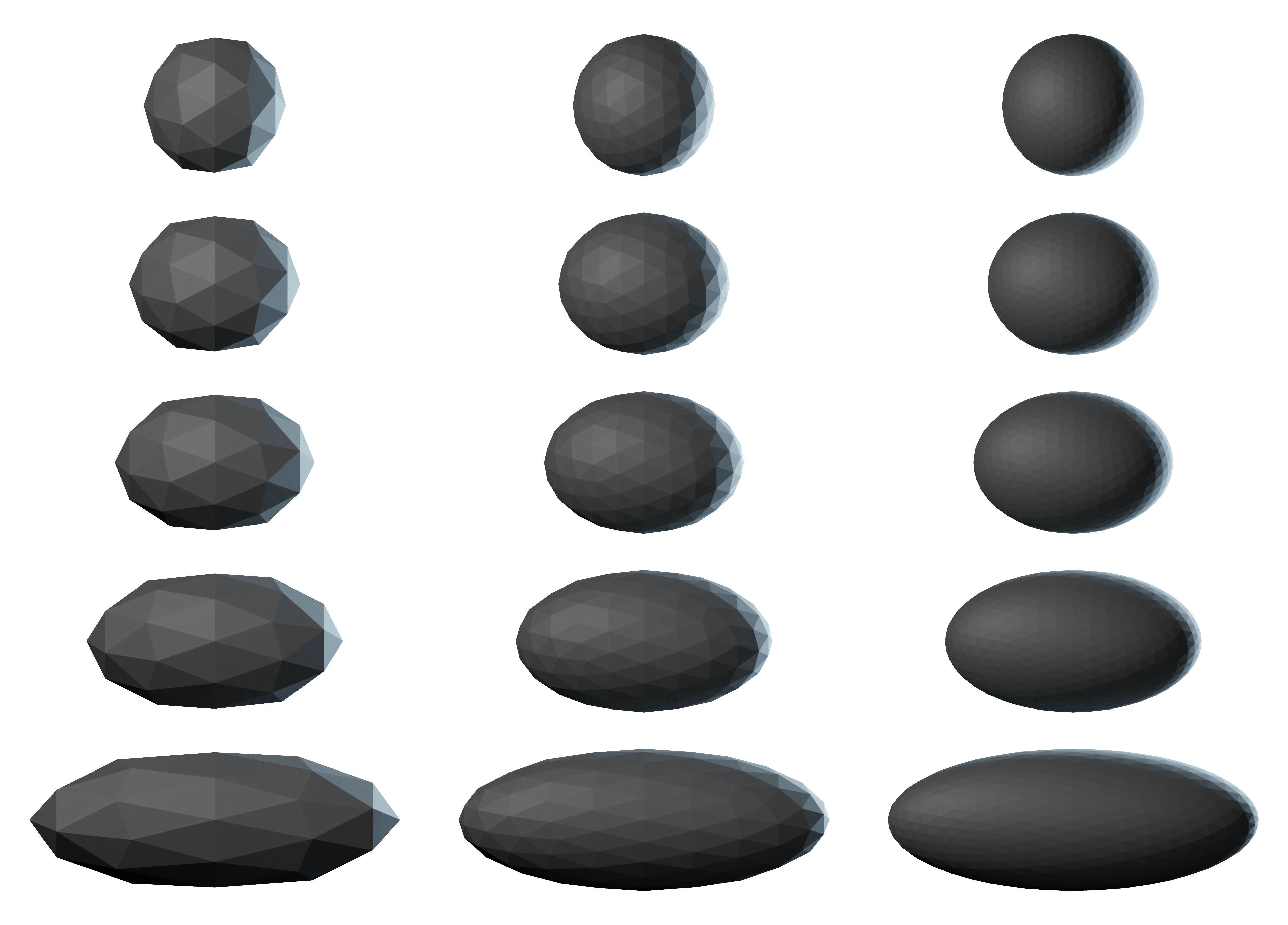
Figure 3: A series of objects created from unit spheres with increasing level of detail ($80\leq|\mathbb{T}|\leq 1,280$ from left to right) and a scale factor ($1.0\leq\eta_{r}\leq 2.6$ from top to bottom).

The combination of $d_{k_{\text{max}}}$ and $\epsilon_{k_{\text{max}}}$ characterises the shape of our coarsest surrogate model. A large diameter relative to a small halo size describes a disc-like object. A small diameter relative to a large halo size describes a sphere-like object. Different triangle counts for the fine grid model allow us to assess the impact of the level of detail of the fine grid mesh onto the resulting coarsest surrogate geometry.

Our surrogate model of choice on the coarsest level (cmp. the penalty term in (6) of the Appendix) almost degenerates to a point if the underlying triangulated geometry approximates a sphere. It approaches a bounding sphere. The triangle count approximating a spherical object does not have a significant qualitative or quantitative impact on this characterisation of the coarsest surrogate triangle. Once the triangulated mesh becomes less spherical, the surrogate triangle starts to align with the maximum extension of the fine mesh. It spreads out within the geometry along the geometry’s longest diameter; an effect that is the more distinct the higher the fine geometry’s triangle count. The halo layer $\epsilon_{k_{\text{max}}}$ around the surrogate triangle, which is analogous to a sphere’s radius if the surrogate triangle approaches a point, remains in the order of $r=0.5$. This is the radius of the original unit sphere ($\eta_{r}=1$).

For a close-to-spherical geometry, our volumetric surrogate model never exceeds 135% of the bounding sphere volume ($|\mathbb{T}|=1,280$). For the highly non-spherical cases ($\eta_{r}=2.6$) our surrogate volume can be as little as $37\%$ ($|\mathbb{T}|=80$) of the simple bounding sphere volume. This advantageous property results from the observation that a growth of $d_{k_{\text{max}}}$ anticipates any extension of the geometry, while the $\epsilon_{k_{\text{max}}}$ ensures that the minimal geometry diameter, which is at least as large as the original sphere, remains covered by the surrogate triangle plus its halo environment.

Observation 1.

For highly non-spherical sets of triangles, our surrogate formalism yields advantageous representations. For spherical observations, it resembles the bounding sphere. This holds for all levels of the surrogate cascade.

In a surrogate tree, fine resolution tree nodes (surrogate triangles) are characterised by the low triangle count measurements in Table 1 where localised patches are highly non-spherical (large $\eta_{r}$). Surrogate triangles belonging to coarser levels inherit characteristics corresponding to larger $|\mathbb{T}|$. We conclude that our triangle-based multiresolution approach is particularly advantageous as an early termination criterion (“there is certainly no collision”) on the rather fine surrogate resolution levels within the surrogate tree, or is overall tighter fitting than bounding sphere formalisms for non-spherical geometries.

6.3 Hybrid single level contact detection

Even though our multiscale approach intends to reduce the number of distance calculations, a high throughput of the overall algorithm continues to hinge on the efficiency of the core distance calculation. We hence continue with studies around the explicit Euler where we omit the multiscale hierarchy. We work with the finest particle mesh representation only.

The assessment of the core comparison efficiency relies on our sphere-on-plane and the particle-particle setup. They represent two extreme cases of geometric comparisons: With the plane, a complex particle with many triangles hits very few triangles. As long as the triangles spanning the plane are large relative to the particle diameter, it is irrelevant how the plane is modelled, i.e. if it consists of solely one or two triangles or an arrangement of multiple triangles. The multiscale algorithms assymptotically approach a $|\mathbb{T}|:1$ comparison with $\mathbb{T}$ given by the particle. When we collide two particles—we use the same triangle count for both—we can, in the worst case, run into a $|\mathbb{T}|:|\mathbb{T}|$ constellation. For both setups, we use strictly spherical particles ($\eta_{r}=1$).

For the triangle-triangle comparisons, two code variants are on the table: We can run the comparison-based (baseline) algorithm, or we can use the hybrid code variant which runs four steps of the iterative scheme before it checks if the two last iterates of the contact point differ by more than $C\epsilon_{h}$. We use $C\approx 1$. If the difference exceeds the threshold, our algorithm assumes that the code has not converged, and hence reruns the comparison-based code to obtain a valid contact assessment. The comparison-based code variant is 4-way vectorised and relies on Intel intrinsics. The hybrid variant is vectorised over batches of eight packed triangle pairs using an OpenMP simd annotation.

Table 2: Particle-particle scenario.. We compare a comparison-based realisation (top) against a hybrid realisation (bottom). Per setup, we present the time-to-solution ([t]=s) per Euler step, i.e. one run through all possible triangle combinations, and we augment these data with MFlop/s rates split up into scalar and vectorised contributions. Vector calculations are categorised as 128 bit packed (SSE) or 256 bit packed (AVX) for four and eight simultaneous 32 bit floating point operations respectively. For the hybrid setup, we finally quantify how many triangle pairs had to be checked a posterio, i.e. as fallback, by the comparison-based algorithm. This runtime is included in the data. All measurements are given as the average per core.

				Packed	Packed
	$|\mathbb{T}|$	Runtime	Scalar	128B	256B	Fallback
Comp.	12	$6.59\cdot 10^{-2}$	$1.52\cdot 10^{-2}$	$3.22\cdot 10^{3}$
	36	$5.17\cdot 10^{-2}$	$1.90\cdot 10^{-3}$	$3.46\cdot 10^{3}$
	140	$3.80\cdot 10^{-1}$	$3.00\cdot 10^{-4}$	$3.18\cdot 10^{3}$
	1,224	$4.35\cdot 10^{1~{}~{}}$	$0.00\cdot 10^{0~{}~{}}$	$3.04\cdot 10^{3}$
Hybrid	12	$4.99\cdot 10^{-2}$	$6.27\cdot 10^{1~{}~{}}$	$1.11\cdot 10^{3}$	$1.07\cdot 10^{4}$	7.7%
	36	$2.76\cdot 10^{-2}$	$1.27\cdot 10^{2~{}~{}}$	$9.69\cdot 10^{2}$	$1.45\cdot 10^{4}$	4.5%
	140	$1.83\cdot 10^{-1}$	$1.97\cdot 10^{2~{}~{}}$	$3.25\cdot 10^{2}$	$1.84\cdot 10^{4}$	1.2%
	1,224	$1.99\cdot 10^{1~{}~{}}$	$2.42\cdot 10^{2~{}~{}}$	$5.30\cdot 10^{1}$	$2.10\cdot 10^{4}$	0.028%

Table 3: Experiments from Table 2 for the particle-on-plane setup.

				Packed	Packed
	$|\mathbb{T}|$	Runtime	Scalar	128B	256B	Fallback
Comp.	12	$2.60\cdot 10^{-2}$	$3.87\cdot 10^{-2}$	$3.33\cdot 10^{3}$
	36	$6.50\cdot 10^{-2}$	$1.96\cdot 10^{-2}$	$3.85\cdot 10^{3}$
	140	$1.84\cdot 10^{-1}$	$1.28\cdot 10^{-2}$	$4.09\cdot 10^{3}$
	1,224	$1.98\cdot 10^{0~{}~{}}$	$2.90\cdot 10^{-3}$	$4.27\cdot 10^{3}$
Hybrid	12	$2.80\cdot 10^{-2}$	$1.06\cdot 10^{1~{}~{}}$	$1.25\cdot 10^{3}$	$9.34\cdot 10^{3}$	6.3%
	36	$6.70\cdot 10^{-2}$	$1.56\cdot 10^{1~{}~{}}$	$1.34\cdot 10^{3}$	$1.19\cdot 10^{4}$	5.1%
	140	$1.79\cdot 10^{-1}$	$2.15\cdot 10^{1~{}~{}}$	$1.34\cdot 10^{3}$	$1.35\cdot 10^{4}$	4.8%
	1,224	$1.85\cdot 10^{0~{}~{}}$	$3.03\cdot 10^{1~{}~{}}$	$9.32\cdot 10^{2}$	$1.48\cdot 10^{4}$	3.6%

Our hybrid approach outperforms a sole comparison-based approach robustly for the $|\mathbb{T}|:|\mathbb{T}|$ setups. For strongly ill-balanced triangle counts, the insulated comparison-based approach is superior (Table 2). The comparison-based code variant is not able to benefit from AVX at all (not shown), while the hybrid AVX usage increases with increasing triangle counts. We end up with up to 40–45% “turbo-mode” peak performance which we have to calibrate with the AVX frequency reduction [7]. The relative number of fallbacks, i.e. situations where the iterative scheme does not converge within four iterations, decreases with growing geometry detail, while the same effect is not as predominant for the particle-on-plane scenario.

Our data confirm the superiority of the hybrid approach for the particle-particle comparisons [15, 16]. They confirm that the approximation of the Hessian does not significantly harm the robustness, even though the number of fallbacks becomes non-negligible. Our arithmetic intensity determines how much improvement results from the hybrid strategy. It is significantly higher for the particle-particle setup as opposed to the particle-on-plane. Therefore, only the former prospers through vectorisation. We see an increased fallback for decreased geometric detail due to the larger relative epsilon, which is used to identify fallback conditions.

Observation 2.

As long as we do not compare extreme cases (single triangle vs. a lot of triangles), the hybrid approach is faster. It is thus reasonable to employ it on all levels of the surrogate tree, even though it might be reasonable to skip iterative comparisons a priori if the coarsest surrogate level is involved. The latter observation does not result from a mathematical “non-robustness” but is a sole machine effect.

6.4 Multiresolution comparisons for explicit time stepping

Within an explicit time stepping code, our multiresolution approach promises to eliminate unnecessary comparisons since it identifies “no collission” constellations quickly through the surrogates: Whenever it compares two geometries, the algorithm runs through the resolution levels top-down (from coarse to fine). The monotonicity of the surrogate definition implies that we can stop immediately if there is no overlap between two surrogates. The code either employs the pure geometry-based approach or the hybrid strategy on all levels. We focus on spherical particles ($\eta_{r}$=1) discretised by 1,224 triangles, and average over 100 time steps such that we run into no-collision phases for the particle-particle setup and see the particle roll down the plane for particle-on-plane.

Table 4: Time-to-solution ([t]=s) and number of triangle distance checks for an explicit Euler step for the particle-particle collision (top) and the particle-on-plane setup (bottom). We compare a comparision-based setup to a hybrid approach on a single level vs. a surrogate hierarchy which is traversed from coarse to fine. For the hybrid configuration, we present the number of comparison-based fallbacks vs. the number of iterative comparisons. Each iterative comparison of two triangles consists of four Newton steps. Only if these four steps fail to converge, the algorithm issues the comparison-based postprocessing. Both the iterative comparisons plus the (fewer) comparison-based postprocessing steps determine the runtime (right column).

	Comparison-based		Hybrid
Method	#tri. comp.	Runtime	#tri. comp.	#iterative	Runtime
Single level	$1.50\cdot 10^{6}$	$3.96\cdot 10^{0~{}~{}}$	$1.66\cdot 10^{3}$	$1.50\cdot 10^{6}$	$1.87\cdot 10^{0~{}~{}}$
Surrogate hierarchy	$8.20\cdot 10^{3}$	$2.60\cdot 10^{-2}$	$1.44\cdot 10^{2}$	$7.64\cdot 10^{3}$	$1.80\cdot 10^{-2}$
Single level	$6.27\cdot 10^{5}$	$1.68\cdot 10^{0~{}~{}}$	$1.57\cdot 10^{4}$	$6.27\cdot 10^{5}$	$8.00\cdot 10^{0~{}~{}}$
Surrogate hierarchy	$5.27\cdot 10^{3}$	$7.68\cdot 10^{-2}$	$4.96\cdot 10^{2}$	$5.03\cdot 10^{3}$	$4.00\cdot 10^{-2}$

Our measurements confirm the superiority of the hybrid scheme in the surrogate context (Table 4): In line with Section 6.3, no multiresolution setup with comparison-based contact detections on surrogate levels is able to outperform the configurations where all levels are tackled through the hybrid approach. Further studies where different variants are used on different (surrogate) levels are beyond scope.

In our two-particles scenario, the particles yield $1,224^{2}$ comparisons per time step if no surrogate helper data structure is used. Our data reflects the quadratic (particle-particle) or linear (particle-on-plane) computational complexity. In both cases, the number of triangle comparisons is reduced by more than an order of magnitude through the surrogate hierarchy, and the surrogate version outperforms its single-level baseline robustly. The hierarchical scheme’s additional computational cost (overhead) is negligible, though it does not significantly alter the ratio of iterative checks to fallback comparisons in the hybrid scheme.

Observation 3.

Our surrogate technique efficiently reduces the number of comparisons between two geometries, as “no-collision” setups are identified with low computational cost.

6.5 Multiresolution comparisons for implicit time stepping

Implicit methods are significantly more stable then their explicit counterpart. The price to pay for this is an increased computational complexity: The Picard iterations that we use imply that we have to run the core contact point detection more often per time step. The Picard iterations’ update of collision point detections imply that the surrogate tree does not unfold linearly anymore. While the explicit time stepping algorithm runs through the tree from coarse to fine, the implicit scheme descends into finer levels yet might, through the iterative updates of the rotation and position, find alternative tree parts that have to be taken into account too or instead. The increased stability of implicit time stepping allows users to pick larger time step sizes which, in practice, compensate to some degree of the increased compute load. This problem-specific cost amortisation is beyond scope here, i.e. we compare implicit and explicit schemes with the same time step size. All data results from spherical particles and the default triangle counts. We average all measurements over 100 time steps and include the “roll down the plane” situation for the particle-on-plane setup.

Table 5: Average number of Picard iterations per time step for our first two scenarios.

	Particle-particle		Particle-plane
Method	Comparison-based	Iterative	Comparison-based	Iterative
Single level or surrogate within Picard	$4.6$	$4.9$	$7.1$	$7.1$
Multiscale Picard	$6.2$	$6.2$	$13.0$	$13.1$

Averaged over 100 time steps, we observe that the number of Picard iterations is small and bounded (Table 5). We study the impact of a switch to the iterative scheme, with the hybrid fallback on the finest level, and observe that it slightly increases the Picard iteration count. The usage of a multiscale method merged into the Picard iterations increases the iteration count, too. Both modifications yield flawed contact point guesses and thus require us to run more Picard iteration steps overall. The wrong guesses have to be compensated later on.

Observation 4.

Both the iterative approximation of contact points and the “one Picard step before we widen the active set” strategy increase the total number of required Picard iterations.

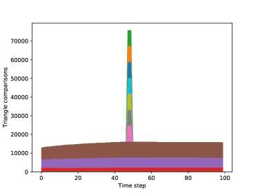
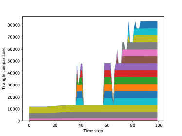
Figure 4: Number of triangle-to-triangle comparisons over time per surrogate representation level. The data stems from the particle-particle (left) and the particle-on-plane setup (right) subject to the implicit time stepping. The lowest layer illustrates the triangle comparison count for the first iteration, the next layer for the second iteration and so forth. The number of layers corresponds to the total number of iterations.

The surrogate hierarchy yields an efficient early termination criterion for our collision detection. If there is no collision, the code does not step down into the fine grid resolutions. This property carries over from the explicit to the implicit algorithm (Figure 4). An increase of the computational cost by a factor of 4.6 is acceptable in return for an implicit scheme. We however observe that this increase holds for brief point contacts only. It raises to a factor of 13.1 if contacts persist. In our example, this happens once the spherical object starts to roll and slide down the tilted plane.

Table 6: Time per time step ([t]=s]) and triangle distance comparisons for our implicit schemes for the particle-particle collision (top) and the particle-on-plane setup (bottom).

	Comparison-based		Hybrid
Method	#tri. comp.	Runtime	#tri. comp.	#iterative	Runtime
Single level	$6.89\cdot 10^{8}$	$1.69\cdot 10^{2~{}~{}}$	$8.78\cdot 10^{5}$	$7.34\cdot 10^{8}$	$7.44\cdot 10^{1~{}~{}}$
Surrogate within Picard	$3.97\cdot 10^{6}$	$1.08\cdot 10^{0~{}~{}}$	$7.14\cdot 10^{4}$	$3.70\cdot 10^{6}$	$7.20\cdot 10^{-1}$
Multiscale Picard	$1.82\cdot 10^{6}$	$7.70\cdot 10^{-1}$	$2.25\cdot 10^{4}$	$1.70\cdot 10^{6}$	$4.70\cdot 10^{-1}$
Single level	$4.43\cdot 10^{8}$	$9.61\cdot 10^{1~{}~{}}$	$1.11\cdot 10^{7}$	$4.43\cdot 10^{8}$	$4.41\cdot 10^{1~{}~{}}$
Surrogate hierarchy	$3.59\cdot 10^{6}$	$4.80\cdot 10^{-1}$	$3.44\cdot 10^{5}$	$3.42\cdot 10^{6}$	$2.20\cdot 10^{-1}$
Multiscale Picard	$3.50\cdot 10^{6}$	$4.90\cdot 10^{-1}$	$3.11\cdot 10^{5}$	$3.35\cdot 10^{6}$	$1.90\cdot 10^{-1}$

Within our multi-resolution framework, the cost per Picard iteration is not uniform and constant but depends heavily on the surrogate tree fragments that are used. The cost are in particular non-uniform for non-simplistic setups. The growth in Picard iterations (on average) per time step (Table 5) increases the number of triangle-to-triangle checks, compared to the explicit schemes (Table 4), by exactly this factor if we stick to a plain geometry model. Yet, it does not manifest in an explosion of the runtime (Table 6) if we employ the surrogate trees. They help to reduce the compute cost dramatically, as we study only those parts of the surrogate tree which might induce a collision. We prune the tree per Picard iteration.

Observation 5.

Our multiscale Picard approach is particularly beneficial for strongly instationary setups where the topology of particle interactions changes quickly.

Permuting and fusing the Picard iteration loops and the traversal over the surrogate tree reduces the number of triangle-to-triangle comparisons further. This observation holds for the particle-particle setup. It does not hold for the particle-on-plane. The advanced version benefits from the fact that we memorise the active set in-between two Picard iterations: While the implicit version from Section 5.2 runs through the whole tree starting from the root in every iteration, our advanced version starts from a certain resolution and unfolds at most one level per Picard step. We save the progress through coarser resolutions, and we do not step all the way down in early iterations. This state-based approach works as our narrowing is effective: if we step down into a “wrong” part of the tree and find out that these fine resolutions do not contribute towards the final force, we successively remove these fine resolutions from the (active) comparison sets again. For a sphere rolling or hopping down a plane, the active set remains almost invariant throughout the Picard iterations, and we do not benefit from the narrowing or an early termination. We do however benefit here from the adaptive localisation of the contact detection within the tree.

Observation 6.

The multiscale Picard approach in combination with a hybrid contact detection keeps the cost of the implicit time stepping bounded by a factor of four compared to an explicit scheme.

6.6 Multiresolution comparisons for implicit time stepping with large scale differences

To assess collisions between objects of different scales, we first instantiate the particle-particle scenario with both particles being spheres approximated by $|\mathbb{T}|=80$ triangles ($\eta_{r}=1$). We fix one of the spheres with a unit diameter, and scale the other one up. All data studies situations where the two particles are close and yield contact points.

Table 7: Time ([t]=s) plus triangle distance comparisons per implicit time step for a particle-particle setup (80 triangles) where one particle is scaled relative to the other one.

Scale	Triangles	Iterations	#tri. comp.	#iterative	Time
1	80	13	$1.59\cdot 10^{1}$	$1.45\cdot 10^{2}$	$8.72\cdot 10^{-2}$
2	80	13	$1.93\cdot 10^{1}$	$1.27\cdot 10^{2}$	$6.80\cdot 10^{-2}$
4	80	18	$4.31\cdot 10^{1}$	$1.78\cdot 10^{2}$	$1.00\cdot 10^{-1}$
8	80	14	$4.10\cdot 10^{1}$	$9.82\cdot 10^{1}$	$6.82\cdot 10^{-2}$

There is no clear trend relating the number of Picard iterations to the scale of the involved particles (Table 7). As the scale difference grows, the number of triangle-triangle comparisons reduces slightly (cmp. how often the iterative scheme is invoked), while more iterative updates run into the fallback, i.e. require a posteriori, if-based triangle comparisons. The cost to compare a large with a small particle thus remains in the same order as the comparison of two equally sized particles. There is no clear runtime trend.

The bigger the size difference between two triangles the more likely it is that the hybrid scheme runs into the fallback (cmp. data in Table 3 where the slope triangles are large compared to the particle triangles). The frequent fallbacks team up with the effect that coarse (surrogate) triangles within the larger particle overlap large numbers of surrogate triangles on the smaller collision partner. Relatively large fractions of the small particle’s surrogate tree have to be unfolded.

Table 8: Time ([t]=s) and triangle distance per time step for two colliding particles of different size with comparable triangle sizes.

Scale	Triangles	Iterations	#tri. comp	#iterative	Runtime
1	80	13	$1.59\cdot 10^{1}$	$1.45\cdot 10^{2}$	$8.72\cdot 10^{-2}$
2	320	19	$4.18\cdot 10^{1}$	$5.05\cdot 10^{2}$	$2.25\cdot 10^{-1}$
4	1,280	20	$4.66\cdot 10^{1}$	$5.88\cdot 10^{2}$	$2.60\cdot 10^{-1}$
8	5,120	17	$3.80\cdot 10^{1}$	$5.44\cdot 10^{2}$	$2.40\cdot 10^{-1}$

To distinguish the impact of the particle sizes from the impact of the triangle, we next subdivide the upscaled colliding particle such that the triangle sizes of both particles remain almost invariant and comparable. Doubling the particle size thus corresponds to four times more triangles. Within the surrogate tree, we keep the number of triangles per leaf roughly constant.

Despite the increase in the number of triangles per upscaling, the number of comparisons and the runtime quickly plateau (Table 8). The additional cost due to the increase in the triangle count is bounded by a factor of four, even if we continue to increase the geometric detail beyond a factor of four. The cost per triangle reduces as one particle grows relative to the other.

As the size of the larger object grows, its surrogate tree becomes deeper. The algorithm unfolds the larger tree, but this unfolding is a localised process. We end up with roughly scale-invariant compute cost which is dominated by the number of triangles stored within one node of the finest tree level.

Observation 7.

The multiscale Picard approach is particularly effective if we compare objects of massively different size yet with the same level of detail. In this case, the cost per triangle comparison remains almost invariant.

The observation is particular encouraging for simulations with objects of massively different size where the large objects exhibit a high level of detail. Such situations are found in fluid-structure interaction, where a collision induces a force on a bending object. Such objects often are modelled via adaptive meshes which have to refine around the contact point.

6.7 Many particle experiments

Our multiscale Picard method shows an improvement in time-to-solution for individual particles which collide with other particles of different size or simple geometric object such as a plane. To be useful in real DEM codes, the algorithms must remain performant when we run simulations with many particles.

As long as the neighbourhood search is efficient, our achievements for individual particle-particle interactions carry over to dynamic simulations with large particle counts. If particles move around and bounce into each other, yet each particle only interacts with few other objects per time step, our multiscale concepts simply are to be generalised from two objects to a small object count. The situation changes if particles enter a stationary regime, i.e. if the particles are densely clustered and almost at rest.

We therefore finally simulate 24,576 particles that barely overlap and are initially at rest. This imitates a basin of granulates, e.g. Each particle is made up of 1,224 triangles, i.e. we handle a total memory footprint of approximately 3.87GiB which is substantially larger than the 30MiB total L3 cache.

Table 9: Measurements for 24,576 particles which are densely clustered yet almost at rest. The runtime is the runtime per time step per core. We present the total time and the time per particle-particle comparison.

	Comparison-based			Hybrid
		Time				Time
Method	#tri. comp.	total	per comp	#tri. comp.	#iterative	total	per comp
Single level	$6.50\cdot 10^{9}$	$1.92\cdot 10^{6~{}~{}}$	$9.67\cdot 10^{2~{}~{}}$	$1.29\cdot 10^{8}$	$6.50\cdot 10^{9}$	$8.36\cdot 10^{5~{}~{}}$	$4.20\cdot 10^{2~{}~{}}$
Surrogate within Picard	$2.49\cdot 10^{6}$	$4.70\cdot 10^{2~{}~{}}$	$2.37\cdot 10^{-1}$	$2.92\cdot 10^{2}$	$2.49\cdot 10^{6}$	$3.77\cdot 10^{2~{}~{}}$	$1.90\cdot 10^{-1}$
Multiscale Picard	$9.08\cdot 10^{5}$	$2.30\cdot 10^{2~{}~{}}$	$1.16\cdot 10^{-1}$	$1.09\cdot 10^{2}$	$1.06\cdot 10^{6}$	$2.13\cdot 10^{2~{}~{}}$	$1.07\cdot 10^{-1}$

The hierarchical scheme yields a massive reduction of (iterative) triangle-triangle comparisions, and it notably succeeds to avoid too many comparisons which subsequently have to be postprocessed (Table 9). The runtime per particle-particle comparison is significantly lower than in previous dynamic setups. Consequently, the cost per particle is lower, too, even though we have around six collision partners per particle.

Since the particles are almost at rest and only have tiny overlaps, the arising forces are very small. Consequently, few Picard iterations are sufficient to converge for the overall setup. The surrogate trees unfold only around the localised contacts, and this unfolding is very efficient, i.e. we barely remove triangles from the active set while we run the Picard iterations.

Observation 8.

The multiscale approach remains advantageous for larger particle assemblies where the particles are densely clustered.

7 Conclusion

We present a family of multi-resolution contact detection algorithms that exhibit low computational cost and high vectorisation efficiency. Few core ideas guide the derivation of these algorithms: We rigorously phrase the underlying mathematics in a multi-resolution and multi-model language where low-cost resolutions (surrogates) or algorithms (iterative contact search) precede an expensive follow-up step which becomes cheaper through good initial guesses or can be skipped in many cases. We replace dynamic termination criteria behind iterative algorithms with fixed iteration counts. While this might mean that we terminate prematurely, a fixed iteration count allowed us to unroll loops and to permute them. The permutation of loops is our last ingredient which we apply on multiple levels: We switch the traversal of triangles with Newton iterations, and we switch the Picard iterations with the tree unfolding.

The present work is solely algorithmic and has theoretical character. A natural next step is its application to large-scale, massively parallel, real-world simulations. This introduces at least three further challenges: First, the parallelisation between multiple compute nodes makes the algorithm more complex and introduces significant upscaling and load balancing challenges. Second, we only use a simple contact model to compute interaction forces which might be inappropriate for actual challenges from sciences and engineering. Finally, our studies solely rely on one, fixed time step size. They do not even employ the fact that implicit schemes allow for larger time step size; a fact which has to be employed and studied for real-world runs. Furthermore, we rely—so far—on a naive assumption that the Picard iterations converge. A more robust code variant would either identify non-convergence via force, rotation and movement deltas that do not decrease over the Picard iterations, or it would exploit the fact that we know how accurate our surrogate models are via their $\epsilon$ value. In both cases, surrogate levels could be skipped automatically.

On the methodological side, there are three natural extensions of our work: First, our surrogate mechanism always kicks off from the surrogate tree’s root when it searches for contact points. For time stepping codes, this is not sophisticated. It might be advantageous to memorise the tree configurations in-between two subsequent time steps and thus to exploit the fact that many particle configurations change only smoothly in time. Scenarios such as our particle-on-plane setup may particularly benefit from this, as coarse level surrogates, where the force estimates are just as likely to push the solution in the wrong direction, can be skipped based on hints from the previous time step.

Second, we work with multiple spatial representations, i.e. accuracies, but we stick to single precision all the way through. It is a natural extension to make our iterative algorithm use a reduced precision on coarse surrogate models, i.e. early throughout the algorithm. Any machine imprecision can be recovered in our case through a slight increase of $\epsilon$. Such a mixed precision strategy is particularly attractive in an era where more and more compute devices are equipped with special-purpose, reduced-precision linear algebra components. An additional flavour of mixed precision arises once we use more complex contact models. It is not clear if such complex models are required on the surrogate levels, too, i.e. it might be appropriate to implement a multi-physics model where surrogate contact detection complements accurate interaction models on the finest mesh level.

Finally, we next will have to tackle large-scale systems implicitly: DEM models are notoriously stiff, yet the stiffness is localised, as typically not all particles in a setup interact with all other particles. It is a natural extension to investigate local time stepping where each particle advances with its own $\Delta t$, and to make the surrogate representations naturally follow and inform these local time step choices.

Appendix A Surrogate triangles

The construction of good surrogate models is a challenge of its own, as there are infinitely many surrogate models for a given particle $p$. We rely a functional minimisation with a fixed coarsening factor to construct the surrogate hierarchy bottom-up. Let one surrogate triangle for a set of triangles $\mathbb{T}_{k-1}$ be spanned by its three vertices $x_{1},x_{2},x_{3}\in\mathbb{R}^{3}$ which follow

$$\operatorname*{arg\,min}_{x_{1},x_{2},x_{3}} \frac{1}{\beta_{\text{size}}}\sum_{x\in\{x_{1},x_{2},x_{3}\},t\in\mathbb{T}_{k-1}}\|x-t\|^{\beta_{\text{size}}}+\frac{\alpha_{\text{area}}}{2}|(x_{2}-x_{1})\times(x_{3}-x_{1})|^{-2}$$

(6) $$+ \frac{\alpha_{\text{inside}}}{\beta_{\text{normal}}}\sum_{x\in\{x_{1},x_{2},x_{3}\},x_{t}\in t\ \forall t\in\mathbb{T}_{k-1}}\left(\max(0,(x-x_{t})\cdot N(x_{1},x_{2},x_{3}))\right)^{\beta_{\text{normal}}}.$$

$\beta_{\text{size}}\geq 2$ is a fixed integer parameter which we usually pick very high, and the term $\|x-t\|$ denotes the distance between a point $x$ and a triangle $t$. The sum thus minimises the maximum distance between the vertices of the surrogate triangle and the triangles from $\mathbb{T}_{k-1}$. We try to make the surrogate triangle as small as possible. The second term acts as a regulariser that avoids that the surrogate triangle degenerates and becomes a single point or a line. Without it, the first term would yield a single point, i.e. $x_{1}=x_{2}=x_{3}$.

The third term exploits the fact that each triangle $t$ of $p$ has a unique outer normal $N(t)$. Even though our surrogate models can be weakly connected, it is thus possible to assign each surrogate triangle an outer normal, too. The penalty term over the scalar product drops out due to the $\max$ function if the surrogate’s normal points into the same direction as the triangles’ normals. Effectively, this term ensures that the surrogate triangle nestles closely around a particle and that spikes do not induce a blown-up surrogate (Fig. 2). Once (6) yields a surrogate triangle, $\epsilon$ is chosen such that the triangle is conservative for $\mathbb{T}_{k-1}$.

Appendix B Surrogate trees

Let $N_{\text{surrogate}}>1$ be the surrogate coarsening factor. We construct a surrogate tree top-down (Algorithm 7):

Algorithm 7 Top-down algorithm to construct a cascade of surrogate models for a given triangulation $\mathbb{T}$. The algorithm yields a tree defined through $\sqsubseteq_{\text{child}}$ and hence allows us to derive a vast set of different, locally adaptive surrogate models.

1:function constructSurrogate($\mathbb{T}$)

2:   Construct surrogate triangle $t$ for $\mathbb{T}$ $\triangleright$ Solve (6)

3:   Assign $t$ smallest $\epsilon$ such that $t^{\epsilon}$ is conservative surrogate

4:   Create trivial graph $\mathcal{T}$ with single node $\{t^{\epsilon}\}$ and no edges

5:   constructSurrogateRecursively($t^{\epsilon},\mathbb{T}$)

6:end function

7:function constructSurrogateRecursively($t^{\epsilon}_{\text{local}}$, $\mathbb{T}_{\text{local}}$)

8:   if $\mathbb{T}_{\text{local}}\leq N_{\text{surrogate}}$ then

9:     Add node $\mathbb{T}_{\text{local}}$ to $\mathcal{T}$

10:     Add edge $\mathbb{T}_{\text{local}}\sqsubseteq_{\text{child}}\{t^{\epsilon}_{\text{local}}\}$ to $\mathcal{T}$

11:   else

12:     Split $\mathbb{T}_{\text{local}}$ into $N_{\text{surrogate}}$ sets $\mathbb{T}_{\text{local},0},\mathbb{T}_{\text{local},1},\mathbb{T}_{\text{local},2},\ldots$ of roughly same size

13:     for $i$ do

14:        Construct surrogate triangle $t_{\text{new}}$ for $\mathbb{T}_{\text{local},i}$ $\triangleright$ Solve (6)

15:        Assign $t_{\text{new}}$ smallest $\epsilon$ such that $t^{\epsilon}_{\text{new}}$ is conservative surrogate over $\mathbb{T}_{\text{local},i}$

16:        Add node $\{t^{\epsilon}_{\text{new}}\}$ to $\mathcal{T}$

17:        Add edge $\{t^{\epsilon}_{\text{new}}\}\sqsubseteq_{\text{child}}\{t^{\epsilon}_{\text{local}}\}$ to $\mathcal{T}$

18:        constructSurrogateRecursively($t^{\epsilon}_{\text{new}},\mathbb{T}_{\text{local},i}$)

19:     end for

20:   end if

21:end function

• The first triangle that we insert into $\mathcal{T}$ is the coarsest surrogate model, i.e. a degenerated object description consisting of one triangle. In line with Definition 4.6, this is the root node of our surrogate tree.

• Recursively dividing creates a tree over sets where all non-leaves have cardinality one. The leaf sets have a cardinality of roughly $N_{\text{surrogate}}$. The number of children per tree node is bounded and typically around $N_{\text{surrogate}}$.

• We construct the surrogate triangles by copying one triangle out of the underlying triangle set. Then, we iteratively minimise the functional (6).

• To obtain surrogates with reasonably small $\epsilon$, we cluster the triangle sets through a tailored $k$-means algorithm [18]. The subsets $\mathbb{T}_{\text{local},i}$ thus are reasonable compact.

There are many alternative paradigms to construct surrogate trees: Bounding sphere hierarchies would be an alternative. Our approach is relatively slow, yet is exclusively used as pre-processing.

References

- [1] T. Akenine-Mller, E. Haines, and N. Hoffman, Real-Time Rendering, Fourth Edition, A. K. Peters, Ltd., USA, 4th ed., 2018.
- [2] F. Alonso-Marroquin and Y. Wang, An efficient algorithm for granular dynamics simulation with complex-shaped objects, (2008), https://arxiv.org/abs/0804.0474.
- [3] F. Alonso-Marroquín and Y. Wang, An efficient algorithm for granular dynamics simulations with complex-shaped objects, Granular Matter, 11 (2009), pp. 317–329.
- [4] K. Apinis, H. Seidl, and V. Vojdani, Enhancing Top-Down Solving with Widening and Narrowing, Springer International Publishing, Cham, 2016, pp. 272–288, https://doi.org/10.1007/978-3-319-27810-0_14, https://doi.org/10.1007/978-3-319-27810-0_14.
- [5] D. Baraff, An introduction to physically based modeling: Rigid body simulation i - unconstrained rigid body dynamics, in In An Introduction to Physically Based Modelling, SIGGRAPH ’97 Course Notes, 1997.
- [6] G. Barequet, B. Chazelle, L. J. Guibas, J. S. Mitchell, and A. Tal, Boxtree: A hierarchical representation for surfaces in 3d, Computer Graphics Forum, 15 (1996), pp. 387–396, https://doi.org/https://doi.org/10.1111/1467-8659.1530387, https://onlinelibrary.wiley.com/doi/abs/10.1111/1467-8659.1530387, https://arxiv.org/abs/https://onlinelibrary.wiley.com/doi/pdf/10.1111/1467-8659.1530387.
- [7] D. Charrier, B. Hazelwood, E. Tutlyaeva, M. Bader, M. Dumbser, A. Kudryavtsev, A. Moskovsky, and T. Weinzierl, Studies on the energy and deep memory behaviour of a cache-oblivious, task-based hyperbolic pde solver, The International Journal of High Performance Computing Applications, 33 (2019), pp. 973–986.
- [8] P. A. Cundall and O. D. L. Strack, A discrete numerical model for granular assemblies, Geotechnique, 29 (1979), pp. 47–65, https://doi.org/10.1680/geot.1979.29.1.47, https://doi.org/10.1680/geot.1979.29.1.47, https://arxiv.org/abs/https://doi.org/10.1680/geot.1979.29.1.47.
- [9] H. Dammertz, J. Hanika, and A. Keller, Shallow bounding volume hierarchies for fast simd ray tracing of incoherent rays, Comput. Graph. Forum, 27 (2008), pp. 1225–1233, https://doi.org/10.1111/j.1467-8659.2008.01261.x.
- [10] C. Eisenacher, G. Nichols, A. Selle, and B. Burley, Sorted deferred shading for production path tracing, Computer Graphics Forum, 32 (2013), https://doi.org/10.1111/cgf.12158.
- [11] C. Ericson, Real-Time Collision Detection.
- [12] S. Gottschalk, M. Lin, and D. Manocha, Obbtree: A hierarchical structure for rapid interference detection, Computer Graphics, 30 (1997), https://doi.org/10.1145/237170.237244.
- [13] M. Held, J. Klosowski, and J. Mitchell, Real-time collision detection for motion simulation within complex environments, in SIGGRAPH ’96, 1996.
- [14] K. Iglberger and U. Rüde, Massively parallel granular flow simulations with non-spherical particles, Computer Science - Research and Development, 25 (2010), pp. 105–113, https://doi.org/10.1007/s00450-010-0114-4.
- [15] K. Krestenitis and T. Koziara, Calculating the minimum distance between two triangles on simd hardware, 4 2015.
- [16] K. Krestenitis, T. Weinzierl, and T. Koziara, Fast dem collision checks on multicore nodes., in Parallel processing and applied mathematics : 12th International conference, PPAM 2017, Lublin, Poland, September 10-13; revised selected papers. Part 1., R. Wyrzykowski, J. J. Dongarra, E. Deelman, and K. Karczewski, eds., no. 10777 in Lecture Notes in Computer Science, 2018, pp. 123–132.
- [17] T. Y. Li and J. S. Chen, Incremental 3D collision detection with hierarchical data structures, Proceedings of the ACM symposium on Virtual reality software and technology 1998 - VRST ’98, 1998 (1998), pp. 139–144, https://doi.org/10.1145/293701.293719.
- [18] J. B. MacQueen, Some methods for classification and analysis of multivariate observations, 1967.
- [19] J. D. McCalpin, Memory bandwidth and machine balance in current high performance computers, IEEE Computer Society Technical Committee on Computer Architecture (TCCA) Newsletter, (1995), pp. 19–25.
- [20] A. D. Rakotonirina and A. Wachs, Grains3D, a flexible DEM approach for particles of arbitrary convex shape - Part II: Parallel implementation and scalable performance, Powder Technology, 324 (2018), pp. 18–35, https://doi.org/10.1016/j.powtec.2017.10.033, https://doi.org/10.1016/j.powtec.2017.10.033.
- [21] E. Shellshear and R. Ytterlid, Fast distance queries for triangles, lines, and points using sse instructions, Journal of Computer Graphic Techniques, 3 (2014), p. 86–110.
- [22] J. Treibig, G. Hager, and G. Wellein, LIKWID: A Lightweight Performance-Oriented Tool Suite for x86 Multicore Environments, in Proceedings of the 2010 39th International Conference on Parallel Processing Workshops, ICPPW ’10, IEEE Computer Society, 2010, pp. 207–216.
- [23] A. Wachs, L. Girolami, G. Vinay, and G. Ferrer, Grains3d, a flexible dem approach for particles of arbitrary convex shape — part i: Numerical model and validations, Powder Technology, 224 (2012), p. 374–389, https://doi.org/10.1016/j.powtec.2012.03.023.
- [24] T. Weinhart, C. Labra, S. Luding, and J. Y. Ooi, Influence of coarse-graining parameters on the analysis of dem simulations of silo flow, Powder Technology, 293 (2016), pp. 138–148.
- [25] S. Zhao and J. Zhao, A poly‐superellipsoid‐based approach on particle morphology for dem modeling of granular media, International Journal for Numerical and Analytical Methods in Geomechanics, (2019).
- [26] W. Zhong, A. Yu, X. Liu, Z. Tong, and H. Zhang, DEM/CFD-DEM Modelling of Non-spherical Particulate Systems: Theoretical Developments and Applications, Powder Technology, 302 (2016), pp. 108–152, https://doi.org/10.1016/j.powtec.2016.07.010, http://dx.doi.org/10.1016/j.powtec.2016.07.010.