Receptive Field Regularization Techniques for Audio Classification and Tagging with Deep Convolutional Neural Networks

Abstract

In this paper, we study the performance of variants of well-known Convolutional Neural Network (CNN) architectures on different audio tasks. We show that tuning the Receptive Field (RF) of CNNs is crucial to their generalization. An insufficient RF limits the CNN’s ability to fit the training data. In contrast, CNNs with an excessive RF tend to over-fit the training data and fail to generalize to unseen testing data. As state-of-the-art CNN architectures – in computer vision and other domains – tend to go deeper in terms of number of layers, their RF size increases and therefore they degrade in performance in several audio classification and tagging tasks. We study well-known CNN architectures and how their building blocks affect their receptive field. We propose several systematic approaches to control the RF of CNNs and systematically test the resulting architectures on different audio classification and tagging tasks and datasets. The experiments show that regularizing the RF of CNNs using our proposed approaches can drastically improve the generalization of models, out-performing complex architectures and pre-trained models on larger datasets. The proposed CNNs achieve state-of-the-art results in multiple tasks, from acoustic scene classification to emotion and theme detection in music to instrument recognition, as demonstrated by top ranks in several pertinent challenges (DCASE, MediaEval).

I Introduction

Convolutional Neural Networks (CNNs) have come to dominate many domains [1], including image classification [2], natural language processing [3, 4, 5], and speech recognition [6]. In computer vision, CNNs have been shown to perform better with deeper architectures [7, 8, 9]. Following this trend, many researchers working on audio tagging and classification tasks have started to employ such deep architectures from vision, by extracting image-like features such as spectrograms [10, 11, 12].

In this work, we show that using deeper architectures which have proven successful in vision tasks do not necessarily guarantee good performance in audio tasks. In particular, we show that deep CNNs designed for vision often have a large Receptive Field (RF) that is not suitable for audio processing tasks, and that such models fail to generalize. We provide solutions to this problem by regularizing the RF of different variants of deep architectures, and we demonstrate that this massively improves results in various audio classification and tagging tasks.

More specifically, we provide generic and systematic methods for controlling the RF of a CNN architecture. Using these, we show how well-known vision architectures can be effectively adapted to the audio domain, by careful RF regularization. We study the effect of RF regularization over the time and the frequency dimensions, individually and jointly, and how the RF size over these dimensions affects the generalization of CNNs. Generally, the experimental results show that the performance is more sensitive to the RF size along the frequency dimension than over time.

As an additional important aspect, we differentiate between (a) the Maximum Receptive Field of a CNN, which can be calculated from its architecture, and (b) the Effective Receptive Field [13] (ERF) of a trained CNN. We introduce a measure for the ERF and analyze the difference to the maximum RF. Finally, we introduce a novel method we call filter damping, that enables us to control the ERF of a CNN, without changing the architectural topology or the filters of the network. We show that filter damping further helps improve generalization by adapting the ERF of models to better fit the task at hand.

We demonstrate all this in large-scale experiments on three different audio classification and tagging tasks–acoustic scene classification; emotion and theme detection in music; musical instrument recognition–and using several datasets, testifying to the generality of the problem and the proposed solution.

As a general lesson, we propose to consider the RF of CNNs as an important hyper-parameter and design factor that should be carefully tuned and investigated when adapting a CNN architecture (which has been designed in other domains such as vision) to the audio world.

The remainder of the paper is structured as follows: after a brief discussion of the related work (Section II), Section III takes a closer look at the concepts of maximum and effective receptive field, and proposes ways to determine and measure them in a given model. We present the studied tasks and the data sets we have chosen for our investigations in Section IV. The presentation of our proposed methods for systematically controlling RF in various deep CNN architectures, and the corresponding experimental investigations, are split into two strands: Sections V and VI focus on the maximum RF, while Sections VII and VIII discuss the ERF. We explain the setup we use to perform the experiments in Appendix A. Finally, Appendix B presents an analysis of the influence of particular components of CNNs on the RF.

II Related Work

With the power of feature learning, CNNs have revolutionized the field of machine vision and image processing. CNNs can learn hierarchies of features, from low-level concepts such as edges to high-level representations of shapes and objects, which contribute to their superior performance.

Several deep CNN architectures have been proposed in the vision domain that have set new milestones. The VGG architectures [7] introduced an effective structure of convolutional and pooling layers that outperformed other models at the time. However, due to the vanishing gradient issue, they were limited in terms of depth (number of processing layers). To address this issue, ResNet [8] and DenseNet [9] architectures were proposed that tackled the vanishing gradient problem by incorporating skip connections to allow better gradient flow through layers and permit the use of very deep architectures.

Despite the success of very deep architectures in the vision world, the audio domain is still dominated by VGG-like architectures [11, 20, 21, 22]. For instance, for the task of acoustic scene classification, Eghbal-zadeh et al. [11] adapted the VGG architecture from computer vision to use spectrograms as input. Their proposed architecture in combination with an i-vector-based system achieved the top rank in DCASE 2016. Hershey et al. [12] compared various well-known image recognition CNN architectures on a large-scale dataset of 70M audio clips from YouTube. They showed that on such a large dataset, very deep CNNs such as ResNet-50 can perform very well. However, deep architectures have shown less success on smaller datasets [23] compared to more shallow architectures such as VGG [24]. As a result, many state-of-the-art acoustic scene classification systems still incorporate shallow CNN architectures [20, 21, 22], since these architectures have been shown to generalize better given the size of the available datasets.

Several neurophysiological studies have focused on understanding the ability of humans and animals to tune their cortical Spectro-Temporal Receptive Fields (STRFs) in order to selectively focus on target sounds, while minimizing the irrelevant acoustics and noise background [25, 26, 27, 28]. Building on such studies, Carlin and Elhilali [25] trained a Gaussian Mixture Model on features obtained from both the initial and adapted STRFs. They showed that an ensemble of adapted STRFs achieves better performance in detecting speech, in the presence of noise. These results suggest that adapting the RF is important, also in biological auditory systems.

Several efforts in the literature have focused on adapting CNNs to audio and music tasks. Pons et al. [29] examined the effect of filter shapes in shallow CNN architectures in music classification tasks and proposed to change the shape of convolutional filters in order to restrict CNNs to learn either temporal or frequency dependencies in the data, which is more relevant to the characteristics of musical signals.

Regarding theme and emotion detection in music, another one of our test domains (see Section IV-B), it is again CNNs that are the most popular models, as evidenced by the submissions to the MediaEval 2019 benchmark [30, 31, 32, 33]. The benchmark baseline [30] uses a VGG-based architecture. Sukhavasi and Adapa [32] use MobileNetV2 [34] with self-attention [35] to capture temporal relations in musical signals. Amiriparian et al [33] use pre-trained CNNs as feature extractors. These CNNs are pre-trained on Audioset [36] as well ImageNet [37] and their extracted features were further used with recurrent NNs as classifiers. Again, we show in this work that RF-regularized CNNs can outperform the aforementioned complex approaches.

Finally, in musical instrument recognition (which we discuss in Section IV-C), a common approach is to use CNNs that are pre-trained on large datasets, and use them as feature extractors to produce embeddings [36, 12], which are then fed into classifiers that map them to the instrument classes [38, 39, 40]. Humphrey et al. [38] use random forests to classify the embeddings, while Gururani et al. [39] study fully connected networks, recurrent neural networks, and an attention-based model. Anhari [40] uses an LSTM [41] with an attention layer to model the instruments. As in the previous cases, we show in the present paper that a simple RF-regularized CNN trained only on OpenMIC can outperform such complex approaches and architectures, including those using models pre-trained on large datasets.

III The Receptive Field of
Convolutional Neural Networks

In this section, we explain two important concepts in CNNs, namely the maximum RF and the Effective RF, which–as shown in later sections–are important for the generalization capabilities of CNNs in audio tasks.

III-A The Maximum Receptive Field of CNNs

A neuron in a convolutional layer is affected only by a part of the layer’s input, as opposed to fully-connected layers, where each neuron takes the whole output of the previous layer as input. In other words, each neuron in a convolutional layer has a specific ‘field of view’. The input of the layer outside of this field of view cannot alter the neuron’s activation. This field of view is known as the Receptive Field (RF).

In this study, we keep our focus on the receptive field over the spatial dimensions of the input (e.g, frequency and time, in the case of spectrograms). In the general case, the output activation of a neuron in a convolutional layer depends on the spatial dimensions of the input and on the channel dimension that represents the number of input feature maps.

We focus on fully-convolutional networks since they have demonstrated superior performance compared to CNNs that incorporate fully-connected output layers [21, 42]. Moreover, a fully-connected layer is equivalent to a convolutional layer with no padding and a filter equal in size to the spatial size of the last feature map. In this section, we start with basic CNN architectures. We detail the more advanced architecture modules in Appendix B.

Within a convolutional layer, the spatial RF of a neuron is determined by its filter size: the larger the filter, the bigger the region of the input it can “see”. The filter size determines the RF of a convolutional layer over the layer input. However, the RF of a layer with respect to the network input (the spectrogram)–that is, what the neuron “sees” of the input–is dependent on the number and configuration of the previous layers as well. The filter size, the stride, and the dilation of all the previous layers influence the RF of a neuron with respect to the input.

In a CNN, the size $RF_{n}$ of the receptive field of a unit from layer $n$ to the network input, along a particular input dimension, can be calculated as:

$$RF_{n} =RF_{n-1}+(k_{n}-1)\cdot S_{n},$$ (1)

$$S_{n} =S_{n-1}\cdot s_{n}$$

where $s_{n}$, $k_{n}$ are stride and kernel size of layer $n$, respectively, and $S_{n}$ is the cumulative stride from layer $n$ to the input layer.

III-B The Effective Receptive Field of CNNs

The previous section described the maximum RF of a neuron, that is, the region of the input that is connected to a neuron. However, parts of the input may have minimal or no influence on the neuron’s activation, depending on the learned parameters of the model. The set of input pixels or units that effectively influence a neuron is called its Effective Receptive Field (ERF). Luo et al. [13] show that neurons are more influenced by input pixels around the center of their max RF, since this region of the input has more paths to the neuron on both the forward and the backward pass. They show that the effective receptive field is different from the theoretical maximum receptive field. Further, they propose a method for computing the Effective Receptive Field (ERF) of a trained CNN, by back-propagating a gradient signal from an output neuron through the network to the input. This method reveals the regions of the input that affect the output the most.

In order to compute the ERF in models trained on audio spectrograms, we follow the approach proposed by Luo et al. [13]. We back-propagate a gradient signal from the output of the penultimate layer to the inputs. Luo et al. [13] visualize the ERF using random data as input, while we use an unseen test set to calculate the gradients with respect to the input. Therefore, we can analyze the relationship between the ERF and the generalization on this unseen test set.

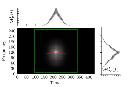
Figure 1: The ERF in white, the maximum RF in green, and our estimates $E_{t}$ and $E_{f}$ in red, for a ResNet with a Maximum RF of $241\times 241$ trained on the DCASE‘18 dataset.

We now propose an objective measure of the ERF size in terms of two scalars $E_{t}$ and $E_{f}$ indicating the ERF size over the time and frequency dimensions, respectively. We define $\mathcal{M}_{\nabla}{(t,f)}$ as the mean of the gradients (over the test set) on an input pixel specified by the pixel coordinates $(t,f)$, where $t$ refers to the coordinate of the time axis, and $f$ represents the pixel coordinate of the frequency axis in the input spectrogram. Let $T$ and $F$ be the dimension, in pixels, of the input along time and frequency, and $\mathcal{M}^{t}_{\nabla}({f})=\sum_{t=1}^{T}\mathcal{M}_{\nabla}{(t,f)}$, $\mathcal{M}^{f}_{\nabla}({t})=\sum_{f=1}^{F}\mathcal{M}_{\nabla}{(t,f)}$ be the marginal sum of the mean gradients over frequency and time dimensions, respectively, as visualized in Figure 1. The ERF size over the time dimension, $E_{t}$, is defined as $E_{t}=4\cdot\sigma_{t}$, where $\sigma_{t}$ is the standard deviation of the marginal sum $\mathcal{M}^{f}_{\nabla}({t})$. We estimate the center of the ERF $\mu_{t}$ and standard deviation $\sigma_{t}$ on the time dimension as shown in  (2):

$$\mu_{t} =\frac{\sum_{t=1}^{T}t\cdot\mathcal{M}^{f}_{\nabla}({t})}{\sum_{t=1}^{T}\mathcal{M}^{f}_{\nabla}({t})},$$

$$\sigma_{t} =\sqrt{\frac{\sum_{t=1}^{T}(t-\mu_{t})^{2}\cdot\mathcal{M}^{f}_{\nabla}({t})}{\sum_{t=1}^{T}\mathcal{M}^{f}_{\nabla}({t})}}$$ (2)

Luo et al. [13] showed that the gradient used in the ERF calculation reaches the maximum value in the center of the Max RF, and the gradient magnitude decays away from the center in a squared exponential way. This can also be observed in our visualisation of the ERF in Figure 1. Given this shape, we can conclude that the range $[\mu_{t}-2\sigma_{t},\mu_{t}+2\sigma_{t}]$ with the length of $E_{t}$, contains most of the impactful pixels, as $E[\frac{\sum_{t=\mu_{t}-2\sigma_{t}}^{t=\mu_{t}+2\sigma_{t}}{\mathcal{M}^{f}_{\nabla}({t})}}{\sum_{t}{\mathcal{M}^{f}_{\nabla}({t})}}]\approx 0.9545$. Therefore, we propose $E_{t}$ as measure of the ERF, as it represent the size of the range that contains the most impactful pixels in the time dimension.

Analogously, we estimate $E_{f}$, the effective ERF size along the frequency axis, by calculating $\mu_{f}$ and $\sigma_{f}$ in a similar fashion to Eq. 2, and defining $E_{f}=4\cdot\sigma_{f}$.

IV Audio Classification and Tagging Tasks

In this section, we introduce the tasks and the respective datasets to be used in our empirical analysis. The tasks, intended to cover a variety of challenges, are acoustic scene classification, emotion and theme prediction in music, and musical instrument recognition.

IV-A Acoustic Scene Classification

The task in Acoustic Scene Classification (ASC) is to classify an acoustic scene (such as city center and park) using a short (10-30 seconds) audio recording. This task has various applications such as content-based multimedia information retrieval, context-aware smart devices and monitoring systems. The evaluation measure commonly used for this task is classification accuracy, as the common benchmark datasets are generally balanced in terms of samples from each class. Accuracy is the official evaluation measure for ASC in the IEEE AASP Challenge on Detection and Classification of Acoustic Scenes and Events (DCASE). The following two recent ASC benchmark datasets are used.

IV-A1 TAU Urban Acoustic Scenes 2018

This dataset was released for the DCASE 2018 Challenge, Task 1 [43], and contains 10-second audio clips recorded from 10 different acoustic scenes. The training data consists of around 1000 minutes of audio. The evaluation (test) data consists of 420 minutes and includes audio clips recorded in cities and countries not included in the training set. Each audio segment must be classified into one out of 10 possible acoustic scenes. We refer to this dataset as DCASE‘18.

IV-A2 TAU Urban Acoustic Scenes 2019

In DCASE 2019 Challenge Task 1 [44], the DCASE’18 acoustic scenes classification dataset was extended by adding audio recorded in 6 new cities. We refer to this dataset as DCASE‘19.

IV-B Emotion and Theme Detection in Music

The goal of this tagging task is to automatically recognize the emotions and ‘themes’ (general concepts or tags such as ‘love’, ‘film’, ‘space’) conveyed in music recordings, which has many applications in Music Information Retrieval (MIR). We use the dataset released in the Emotion and Theme Recognition in Music Task at the MediaEval-2019 Challenge. This is a subset of the MTG-Jamendo dataset [30], which we refer to as MediaEval-MTG-Jamendo dataset throughout this paper. The subset consists of 9,949 and 4,231 recordings for training and testing, respectively. Each recording is tagged with one or more out of 57 possible labels.

We use Precision-Recall Area Under Curve (PR-AUC) as the performance measure for this task. PR-AUC accounts for different decision threshold values, and was the official evaluation measure in the MediaEval challenge.

IV-C Musical Instrument Recognition

Instrument recognition is the task of recognizing the presence of musical instruments in an audio clip. We focus our study on polyphonic instrument recognition, where multiple instruments are present in the signal. This is considered to be significantly more difficult [45, 39, 46, 47] than monophonic instrument recognition, where the task is to recognize the instrument from a note or an audio signal containing a single instrument.

OpenMIC-2018 [38] is a freely available dataset of 20,000 audio clips from the Free Music Archive [48]. Each clip is 10 seconds long and is annotated with tags indicating the presence or absence of 20 possible instruments. Because multiple instruments can appear in a single clip, this is a multi-label instrument recognition problem. The dataset is known to be noisy because of the particular way the ground truth tags were collected via crowd-sourcing, leading to a potentially large fraction of missing labels and annotator disagreements.

V Controlling the Max RF

Equation (1) in Section III shows that we can control the RF of a basic CNN by changing the number of layers $N$ and the filter size $k_{n}$ and stride $s_{n}$ of a layer $n$. In Appendix B, we investigate some of the widely-used components that are commonly used in famous CNN architectures, and discuss how they relate to the change in the Max RF. In this section, we propose a method to systematically control the RF of two CNN architectures, and explain our proposed RF-regularized CNNs in Section V-A. These two architectures are the basis of our experiments. In Section V-B, we extend our method to control the Max RF on each dimension independently, which allows us to investigate the impact of the Max RF in time or frequency separately.

V-A RF-Regularized CNNs

V-A1 ResNets

ResNet [8] is a very well-known CNN architecture that enables the architecture to be very deep while maintaining the gradient flow, by incorporating residual connections between layers. ResNet variants exhibited state-of-the-art performance in many computer vision tasks [49]. However, as explained in Section III, the Max RF of CNNs tends to grow as the networks go deeper, by stacking more layers. A larger RF–as we will show–hinders the CNN’s ability to generalize in audio tasks.

We control the Max RF of a ResNet by changing the filters of a number of its convolutional layers from $3\times 3$ to $1\times 1$, since $1\times 1$ filters do not increase the Max RF of the network (see Equation (1)). We call the resulting architecture family CP_ResNet. The Max RF of a CP_ResNet is controlled by a hyper-parameter $\rho$, which determines the number of $3\times 3$ and $1\times 1$ filters. The resulting CP_ResNet architecture consist of a $5\times 5$ convolutional layer followed by a $3\times 3$ layer, a $1\times 1$ layer and $2\times 2$ pooling. This is then followed by $\rho$ layers with $3\times 3$ filters and $(21-\rho)$ layers with $1\times 1$, as specified in Table I and Equation 3:

$$x_{k}=\begin{cases}3&\quad\text{if }k\leq\rho\\ 1&\quad\text{if }k>\rho\\ \end{cases}$$ (3)

Values of $\rho$ ranging from 0 to 21 result in networks with a Max RF ranging from $23\times 23$ to $583\times 583$, as shown in Table II.

TABLE I: CP_ResNet architectures family

RB Number	RB Config
	Input $5\times 5$ stride=$2$
1	$3\times 3$, $1\times 1$, P
2	$x_{1}\times x_{1}$, $x_{2}\times x_{2}$, P
3	$x_{3}\times x_{3}$, $x_{4}\times x_{4}$
4	$x_{5}\times x_{5}$, $x_{6}\times x_{6}$, P
5	$x_{7}\times x_{7}$, $x_{8}\times x_{8}$
6	$x_{9}\times x_{9}$, $x_{10}\times x_{10}$
7	$x_{11}\times x_{11}$, $x_{12}\times x_{12}$
8	$x_{13}\times x_{13}$, $x_{14}\times x_{14}$
9	$x_{15}\times x_{15}$, $x_{16}\times x_{16}$
10	$x_{17}\times x_{17}$, $x_{18}\times x_{18}$
11	$x_{19}\times x_{19}$, $x_{20}\times x_{20}$
12	$x_{21}\times x_{21}$, $x_{22}\times x_{22}$
RB: Residual Block, P: $2\times 2$ max pooling.
$x_{k}\in\{1,3\}$: is determined by $\rho$ (Equation 3)
of the network. Number of channels per RB:
128 for RBs 1-4; 256 for RBs 5-8; 512 for RBs 9-12.

TABLE II: Mapping $\rho$ values to the maximum RF (applies to both CP_ResNet and CP_DenseNet).

$\rho$ value	Max RF	$\rho$ value	Max RF
0	$23\times 23$	1	$31\times 31$
2	$39\times 39$	3	$55\times 55$
4	$71\times 71$	5	$87\times 87$
6	$103\times 103$	7	$135\times 135$
8	$167\times 167$	9	$199\times 199$
10	$231\times 231$	11	$263\times 263$
12	$295\times 295$	13	$327\times 327$
14	$359\times 359$	15	$391\times 391$
16	$423\times 423$	17	$455\times 455$
18	$487\times 487$	19	$519\times 519$
20	$551\times 551$	21	$583\times 583$

TABLE III: CP_DenseNet architectures family

Convolutional Layers Config

Input $5\times 5$ stride=$2$

B $3\times 3$ C , B $1\times 1$ C, B P

B $x_{1}\times x_{1}$ C, B $x_{2}\times x_{2}$ C, P

B $x_{3}\times x_{3}$ C, B $x_{4}\times x_{4}$

B $x_{5}\times x_{5}$ C, B $x_{6}\times x_{6}$ C, P

B $x_{7}\times x_{7}$ C, B $x_{8}\times x_{8}$ C B $x_{9}\times x_{9}$ C, B $x_{10}\times x_{10}$ C

B $x_{11}\times x_{11}$ C, B $x_{12}\times x_{12}$ C B $x_{13}\times x_{13}$ C, B $x_{14}\times x_{14}$ C

B $x_{15}\times x_{15}$ C, B $x_{16}\times x_{16}$C B $x_{17}\times x_{17}$ C, B $x_{18}\times x_{18}$ C

B $x_{19}\times x_{19}$ C, B $x_{20}\times x_{20}$ C B $x_{21}\times x_{21}$ C, B $x_{22}\times x_{22}$ C

B: $1\times 1$ convolution, P: $2\times 2$ max pooling.

C: Concatenating the input of the DenseLayer.

A Dense layer consists of B $x\times x$ C.

$x_{k}\in\{1,3\}$: is determined by $\rho$ (Equation  3)

V-A2 DenseNets [9]

are another successful architecture with state-of-the-art performance in many computer vision tasks. Similar to ResNets, DenseNets use skip connections to allow the back-propagation of a stronger learning signal to the first layers.

Dense layers are the building block of DenseNets [9]. Each Dense layer consists of two convolutional layers: the first projects the input using $1\times 1$ filters and therefore does not affect the Max RF. The second convolutional layer uses $3\times 3$ filters that increase the Max RF. The growth rate is a hyper-parameter that determines the number of channels in the output of each Dense layer. This output will be concatenated to the layer’s input and passed as input to the next layers.

We construct CP_Dense by choosing the filter sizes in the Dense layers according to a parameter $\rho$, which controls the number of $3\times 3$ convolutions in the Dense layers that are changed to $1\times 1$, in a similar fashion in CP_ResNet. Table III and Equation (3) define the final architecture for a $\rho$ value. Table II shows the Max RF for both CP_DenseNet and CP_ResNet.

The output of each Dense layer is connected to all the following Dense layers, and therefore contributes to increasing the Max RF of the network. However, the growth rate does not change the Max RF, since it only affects the number of filters in each Dense layer.

V-A3 VGG baseline

We use the shallow VGG-like architecture proposed by [21] as a baseline. The network has a max RF of $135\times 135$ pixels.

V-B Controlling RF Dimensions Separately

In order to analyze the impact of the Max RF over a single dimension (time or frequency), we need to control this dimension independently. We accomplish this by extending the proposed method, using two independent hyper-parameters $\rho_{f}$ and $\rho_{t}$ to control the Max RF over the frequency and the time dimension, respectively. We replace CP_ResNet filters (Table I) in the $k^{th}$ layer from $x_{k}\times x_{k}$ with $x_{k}^{f}\times x_{k}^{t}$, where $x_{k}^{f}$ and $x_{k}^{t}$ are controlled by $\rho_{f}$ and $\rho_{t}$, respectively, as shown in Equation 4:

$$x_{k}^{d}=\begin{cases}3&\quad\text{if }k\leq\rho_{d}\\ 1&\quad\text{if }k>\rho_{d}\\ \end{cases}$$ (4)

where $d$ is either the time or the frequency dimension.

VI The Impact of the Max RF on Generalization

In this section, we evaluate and analyze the prediction and generalization capabilities of CNNs under various Max RF settings. In Section VI-A, we show that CNNs with large RFs show signs of overfitting. We evaluate the CNNs on the studied tasks in Section VI-B. Further, in Section VI-C, we analyze the impact of the RF size on each dimension independently.

VI-A Overfitting the Training Data

We first look at an experiment that indicates that although CNNs with larger RF fit the training data better, they fail to generalize to the test data after a certain limit. We analyze the impact of changing the Max RF on the training and testing loss of a CP_ResNet on an acoustic scene classification task, using the DCASE’18 dataset (Section IV). We train variants of CP_ResNet (Section V-A1) with different Max RF settings. Figure 2 shows the training and testing loss of the model, as the Max RF increases. While we can see that increasing the max RF always results in a decrease in the training loss, this is not the case for the testing loss. As the max RF continues to grow larger than 200, the testing loss starts to rise. This indicates that while the CNN’s capability to fit the training data has been increased by growing the Max RF, the model starts to overfit if the Max RF becomes very large. Figure 15 in Appendix B shows the same effect when increasing the Max RF without changing the number of parameters of the CNN.

Figure 2: Training loss vs. testing loss of a CNN with different Max RFs. The increase of the testing loss with larger Max RF indicates overfitting.

VI-B Performance on Audio Classification and Tagging Tasks

Figure 3: Testing accuracy of CP_Dense and CP_ResNet on DCASE‘18. The Max RF size of the network over both time and frequency dimensions (x-axis) ranges from $23\times 23$ to $551\times 551$

In this section, we present the results of training CP_ResNet and CP_DenseNet on the three studied tasks introduced in Section IV.

VI-B1 Acoustic Scene Classification

Figure 3 shows the prediction accuracy of CP_ResNet and CP_DenseNet models on the test part of the DCASE‘18 dataset, with a growth rate of $64$. The plots show that both architectures achieve the best performance in the range of approximately $100\times 100$ to $200\times 200$ pixels. When the Max RF goes below this range, performance degrades. This can be explained by the fact that the network underfits the training data as shown in Figures 2 and 15. In contrast, as the Max RF goes beyond the optimal range, the networks show signs of overfitting and therefore degrade in performance. It is worth noting that the average accuracy of CP_ResNet_ρ=5 $0.779$ lies within the 95%-confidence interval of the VGG baseline $[0.747,0.780]$, while the average performance of CP_DenseNet_ρ=6 $0.781$ lies outside this interval.

TABLE IV: Accuracy Comparison of CP_ResNet with the state of the art on the DCASE‘19 Dataset

Method	Seen Cities	Unseen Cities	Overall
Chen et al. [42]	86.7 %	77.9 %	85.2 %
CP_ResNet CV	84.8 %	78.5 %	83.7 %
CP_ResNet Single	84.2 %	75.8 %	82.8 %
Seo et al. [50]	83.8 %	76.5 %	82.5 %

Table IV offers a performance comparison between the state-of-the-art models in acoustic scene classification, based on the submissions to the DCASE 2019 challenge[44]. We show the results on both the unseen cities (no recordings from these cities were present in the training set), seen cities, and the total accuracy. Chen et al. [42] achieved the first place using an ensemble of 9 different models (including different CNNs and RNNs), trained on different types of input features. They utilize a complex data augmentation scheme using Auxiliary Classifier Generative Adversarial Network (ACGAN) [51] and Conditional Variational Autoencoder (CVAE) [52] and adversarial training as domain adaptation techniques, for a better generalization to unseen cities. Seo et al. [50] achieved third place in the challenge using an ensemble of 8 models consists of 3 types of CNNs trained on various types of pre-processed input features. CP_ResNet-based submissions achieved second place in the challenge. In addition, a single model CP_ResNet trained on the whole training set (“CP_ResNet Single” in the table) reaches comparable performance.

Further results for the CP_DenseNet with different growth rates can be found in Figure 16 in Appendix B. Additionally, the class-wise performance of CP_ResNet on DCASE‘19 and a comparison with the SOTA are provided in Table VII. We refer the reader to [53, 15] for detailed results on DCASE 2016, DCASE 2017 and DCASE 2019 datasets.

VI-B2 Emotion and Theme Recognition in Music

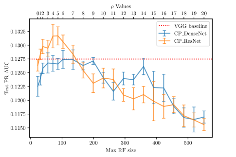
Figure 4: PR_AUC of CP_Dense and CP_ResNet on MediaEval-MTG-Jamendo test set. The Max RF size of the network over both time and frequency dimensions (x-axis) ranges from $23\times 23$ to $551\times 551$

Figure 4 shows the Precision-Recall Area Under Curve (PR_AUC) for CP_ResNet and CP_DenseNet trained on the MediaEval-MTG-Jamendo Dataset (see Section IV-B). The plots show that the optimal Max RF range for this tagging task in CP_ResNet is approximately between $50$ pixels and $100$. CP_DenseNet has a wider Max RF range where it maintains its best performance before degrading in larger RF experiments.

TABLE V: Performance Comparison of the state of the art on the test set of MediaEval-MTG-Jamendo Dataset

Method	PR_AUC
RF-Reg. CNNs Ensemble*	.1546
CP_ResNet${}_{\rho=5}\dagger$	.1312$\pm.0017$
CP_DenseNet${}_{\rho=9}\dagger$	.1271$\pm.0006$
SS CP_ResNet${}_{\rho=9}\dagger$	.1395$\pm.0013$
Sukhavasi and Adapa [32]*	.1259
Amiriparian et al [33]*	.1175
VGG Baseline (ours) [21]	.1275$\pm.0015$
Baseline [30]*	.1077
$\dagger$: single model, not submitted to the challenge.
*: Results taken from the challenge.
SS: Shake-Shake

Table V offers a comparison of the state-of-the-art methods on emotion and theme recognition in music, based on the models submitted to the MediaEval 2019 Challenge. Sukhavasi and Adapa [32] used MobileNetV2 [34] with self-attention [35]. Amiriparian et al [33] used pre-trained CNNs and RNNs. Our submission, under “RF-regularized CNNs Ensemble” [31], consisted in of an ensemble of CP_ResNet, CP_FAResNet, and Shake-Shake regularized CNNs as explained in Appendix B. As can be seen in Table V, our model achieved first place in the challenge by a considerable margin, in terms of PR_AUC. Rows 2-4 in the table refer to the three individual component models of our ensemble, which were not submitted to the challenge but still seem to surpass the other submissions. These results strongly suggest that RF-regularized CNNs are capable of achieving top performance, without pre-training, attention, or recurrent modules.

VI-B3 Musical Instrument Tagging

Figures 5 and 6 show PR-AUC and F-score on the test part of the OpenMIC [38] dataset. The figures show that the optimal Max RF for both architectures is approximately between $50$ and $100$ pixels. Similar to the results in the previous tasks, we can see that the performance of both architecture families degrades rapidly as the Max RF of the networks grows.

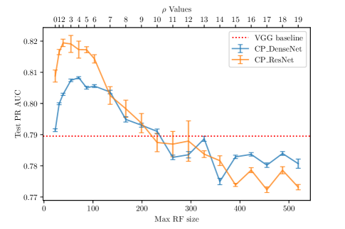
Figure 5: PR-AUC of CP_Dense and CP_ResNet on OpenMIC dataset. The Max RF size of the network over both time and frequency dimensions (x-axis) ranges from $23\times 23$ to $551\times 551$

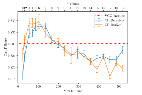
Figure 6: F-Score of CP_Dense and CP_ResNet on OpenMIC dataset. The Max RF size of the network over both time and frequency dimensions (x-axis) ranges from $23\times 23$ to $551\times 551$

TABLE VI: Performance comparison of the state-of-the-art on the test set of OpenMIC (cited methods are sorted by publication date).

Method	PR_AUC	F-scoreb	F-scorea
CP_ResNetρ=3	.819$\pm.001$	.809$\pm.003$	.847$\pm.002$
SS CP_ResNetρ=7	.831$\pm.000$	.822$\pm.001$	.855$\pm.002$
Castel-Branco  [54]	.701	-	-
Anhari [40]	-	-	.83c
Gururani [39]	-	.81c	-
Baseline [38]	.795	.785	.826
VGG Baseline (ours) [21]	.789$\pm.003$	.801$\pm.001$	.83$\pm.002$

• Classical F-score as used in [40, 38]

• Average of the F-score of the positive and negative class per instrument as proposed in  [39]

• Indicates that the number is approximately read from the figures in the referenced papers

• SS: applying Shake-Shake regularization.

Table VI shows the state-of-the-art in instrument tagging in polyphonic music on the OpenMIC dataset. All of the previous state-of-the-art approaches [40, 39, 38] use CNNs pre-trained on the Audioset dataset [36]. They then train an audio tagging model using the CNN’s embedding as input, which in [38] is a random-forest, in [39] is an attention module, and in  [40] is an RNN with attention. Comparing these to our CP_ResNets, we again see that simple RF-regularized CNNs can achieve at least comparable performances without using larger external datasets, pre-training, or stacking additional classification models.

VI-C Studying the Influence of the Time and Frequency Dimensions Independently

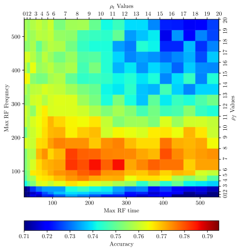
Figure 7: Test set accuracy of different variants of CP_ResNet with changing Max-RF over time (x-axis) and frequency (y-axis). Max-RF ranges from $23\times 23$ to $551\times 551$

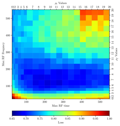
Figure 8: Loss on test set of different variants of CP_ResNet with changing Max-RF over time (x-axis) and frequency (y-axis). Max-RF ranges from $23\times 23$ to $551\times 551$

The previous experiments showed the impact of changing the Max RF over both the frequency and the time dimension of the spectrograms. In this section, we analyze the impact of the Max RF in the two dimensions independently. We study the modified version of CP_ResNet (as explained in Section V-B) by testing instances of CP_ResNet with various $\rho_{f}$ and $\rho_{t}$ values on the DCASE’18 dataset.

Figures 7 and 8 show the test set accuracy and loss for different Max RF values over each of the dimensions. We can see that a Max RF approximately between $100$ and $200$ over the frequency, correlates with the highest performance (similar to our findings in Figure 3). Furthermore, as long as Max RF over the frequency dimension is within this range, increasing the Max RF over the time dimension has only minor effects on the performance.

The two figures also show that too small a Max RF over frequency (below $55$ pixels) generally results in poor performance. However, this can be partly compensated for by choosing a large RF over time (see the bottom strip in the figures) – at least in this particular task.

VII Controlling the Effective RF

In this section, we investigate restricting the ERF while keeping other factors of a CNN – such as architecture, topology, number of parameters – constant. We achieve this by modifying a CNN with a specific Max RF. We decay the influence of the input, the further the input is from the center of the RF. This process does not affect the Max RF of the CNN but decreases the size of its ERF (Section III-B). We call the resulting networks damped CNNs. We damp all the filters of a convolutional layer by performing an element-wise multiplication of the kernel with a constant matrix $C\in\mathbb{R}^{T\times F}$ before apply the convolution operator. We call $C$ the damping matrix. The damping matrix has the same spatial shape as the filter and works by weakening the effect of spatially-outermost weights of the filter. In other words, we replace every convolution operation $O_{n}=W_{n}\star Z_{n-1}+B_{n}$ with $O_{n}=(W_{n}\odot C_{n})\star Z_{n-1}+B_{n}$, where $\star$ is the convolution operator, $\odot$ is the Hadamard product, $Z_{n-1}$ is the output of the previous layer, $W_{n}$ and $B_{n}$ are the weight and bias of the layer $n$.

For our experiments, we choose a damping matrix $C\in\mathbb{R}^{T\times F}$ whose elements are given by the following equation:

$$c_{t,f}=\left(1-m_{t}\frac{\mathopen{|}t-T/2\mathclose{|}}{T/2}\right)\left(1-m_{f}\frac{\mathopen{|}f-F/2\mathclose{|}}{F/2}\right)$$ (5)

where $t\in\{0,\dots,T-1\}$, $f\in\{0,\dots,F-1\}$ are the matrix element indices, $T$, $F$ are the filter sizes over time and frequency respectively. $m_{f}$, $m_{t}$ are hyper-parameters that control the damping in each dimension. Multiplying the weights with the damping matrix $W_{n}\odot C_{n}$ is equivalent to scaling the weights (corresponding to the outer regions of the Max RF) to smaller values, and scaling their gradients down without changing any other factor in the training setup. Therefore, damping can be seen as an inductive bias hindering the network from fitting the outer regions of its max RF during training. Moreover, damping uses element-wise multiplication with the weights during training which has linear complexity with respect to the number of parameters and negligible computationally compared to the matrix multiplications and convolution operations. After training, the weights can be updated by multiplying with the damping matrix, and therefore no additional computational complexity is added at inference time.

Similar to the experiments on controlling the Max RF, we investigate the effect of damping in both dimensions simultaneously, or separately.

VII-1 Damping on Both Dimensions

We set $m_{t}=m_{f}=0.9$, which means that $C$ decays linearly away from the center along each dimension, scaling down the effects of input pixels further from the center in each dimension.

VII-2 Damping on the Frequency Dimension

In these experiments, we set $m_{t}=0,m_{f}=0.9$, which results in a linear decay of $C$ away from the center only over the frequency dimension. This scales down the effects of the input pixels with distance from the center in the frequency dimension while keeping the influence of the input regardless of the distance from the center over the time dimension.

VII-3 Damping on the Time Dimension

This similar to the previous section but done on the time dimension.

VIII The Impact of the ERF on Generalization

In this section, we present the results of restricting the ERF of the CP_ResNet.

VIII-A Performance on Audio Classification and Tagging Tasks

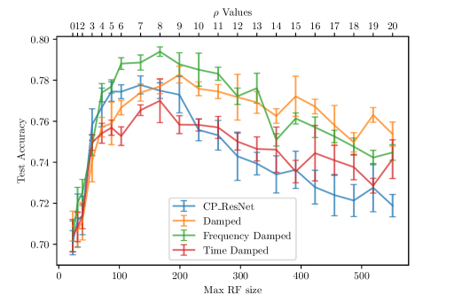
Figure 9: Testing accuracy on DCASE‘18 of CP_ResNet and variants with damped filters over time dimension (Time Damped), frequency dimension (Frequency Damped) or both dimensions (Damped). The 4 networks have the same Max RF for a $\rho$ value but differ by the ERF size.

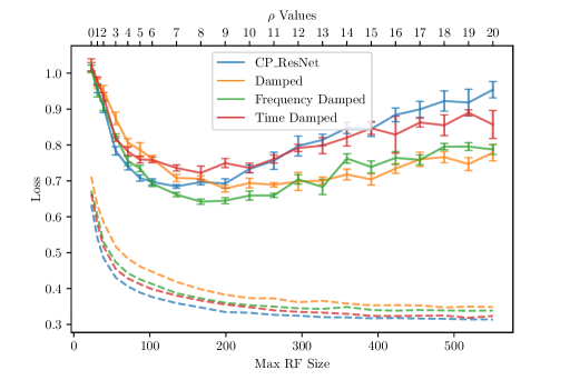
Figure 10: Comparing Testing loss (solid lines) and training loss (dashed lines) on DCASE‘18 of CP_ResNet and variants with damped filters. The 4 networks have the same Max RF for a $\rho$ value but differ by the ERF size.

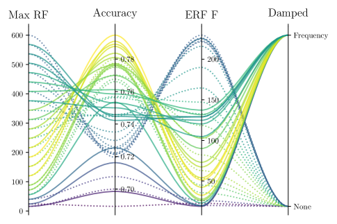
Figure 11: Comparing the ERF over frequency (ERF F) and accuracy on DCASE‘18 of a CP_ResNet with damped filters over the frequency dimension (solid lines) vs with no damping (dashed lines). The color of the lines indicates the accuracy as can be read from the accuracy axis.

In this section, we present the results of our experiments with the damped CP_ResNets. We calculate the Max RF size as explained in Section III-A, and additionally, calculate the ERF size as explained in Section III-B.

Figures 9 and 10 show the influence of restricting the ERF by damping, on the performance of the CNN. As can be seen, the damped variants perform better than the non-damped ones as the Max RF grows larger. Additionally, the “Frequency-Damped” CNNs significantly outperform the original network on this task, indicating the importance of the inductive bias introduced by damping. This also indicates that restricting the RF (both ERF and Max RF) over the frequency dimension has a higher impact on generalization, for the task of ASC. Figure 10 shows that the damped networks have a larger loss on the training data but generalize better on the test data.

Figure 11 shows the correlation between the accuracy and the ERF size over frequency (ERF F) for both CP_ResNet and CP_ResNet with damped filters over the frequency dimension. While both networks have identical Max RF for a given configuration ($\rho$ value), damping helps in restricting the ERF (over the frequency dimension) to the optimal range. In larger Max RF settings, the ERF size of the frequency damped version is significantly smaller, and therefore a larger range of Max RF settings (50, 450) have the optimal ERF achieving a minimum accuracy of $.76$, compared to the Max RF range of (50, 200) in the non-damped case. Thus, filter damping can be considered as a simple but powerful tool for improving generalization on this task.

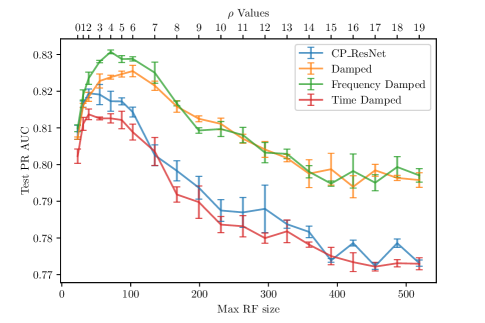
Figure 12: PR-AUC of CP_ResNet and the damped variants on OpenMIC dataset. The Max RF size of the network over both time and frequency dimensions.

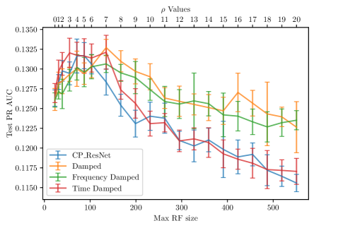
Figure 13: PR-AUC of CP_ResNet and the damped variants on MediaEval dataset. The Max RF size of the network over both time and frequency dimensions.

Figure 12 shows a similar pattern on OpenMic dataset; damping over both dimensions and over the frequency dimension reduce overfitting as the Max RF increases. Furthermore, frequency damping boosts the performance of CP_ResNet_ρ=4 to the state-of-the-art performance of SS CP_ResNet_ρ=7. The same trend can also be seen in Figure 13 on the MediaEval-MTG-Jamendo Dataset.

VIII-B Relationship between RF-Regularization and the Number of Parameters

Many factors influence the ability of CNNs to generalize, such as width and depth [55], network architecture, and the number of parameters [56]. Changing any of these will have an effect on the capacity of the network to fit the training data and to generalize to unseen data.

In Figures 9, 12 and  13, for every $\rho$ value, CP_ResNet and its three damped variants have the same number of parameters and the same topology. The performance improvement can be explained by the difference in the size of the ERF between the four models. We influence the size of the ERF by introducing damping.

Both Figures 2 and 15 show the same pattern when comparing the training and testing loss of ResNets. However, in Figure 15 all the networks have the same number of parameters; they only differ by the number of pooling layers.

The max RF regularization method (as proposed in Section V) works by changing the filter sizes to restrict the RF of the CNN. Changing the filter sizes of a convolutional layer from $3\times 3$ to $1\times 1$ does change the number of parameters of the layer from $3\times 3\times C_{in}\times C_{out}$ to $1\times 1\times C_{in}\times C_{out}$, where $C_{in}$, $C_{out}$ are the number of input and output channels respectively. In order to disentangle the number of parameters from the Max RF, we use grouped convolutional layers [57]. Using grouped convolution does not change the max RF of the network, but rather changes the RF of a layer over its input channels. In other words, grouped convolutional layers can be seen as: first, slicing the input over the channels dimension to $g$ groups, each with $C_{in}/g$ channels; second, applying the convolution operator on each group resulting in $C_{out}/g$ each; and finally, concatenating the output of the $g$ groups over the channels dimension, resulting in $C_{out}$ channels. As a result, it changes the number of parameter of every layer from $X_{t}\times X_{f}\times C_{in}\times C_{out}$ to $g\times X_{t}\times X_{f}\times(C_{in}/g)\times C_{out}/g=X_{t}\times X_{f}\times C_{in}\times C_{out}/g$, where $X_{t}$,$X_{f}$ are the filter size over time and frequency respectively, and $g$ is the number of groups. In short, grouping is a simple method to reduce the number of parameters without affecting the spatial max RF of the CNN. Figure 14 compares the accuracy on DCASE‘18 and number of parameters of CP_ResNet with variants with grouped convolutional layers using 4 groups and 8 groups. The figure shows that the accuracy of the networks is correlated with the RF and not with the number of parameters.

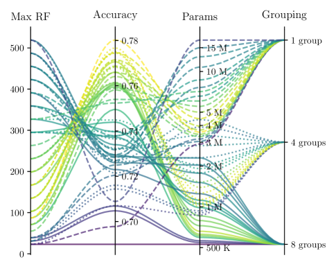
Figure 14: Comparing the accuracy, number of parameters, and Max RF variants of CP_ResNet with grouped convolutional layers on DCASE‘18.

IX Conclusion

In this paper, we have analyzed the impact of the maximum and the effective receptive field on the generalization capability of deep convolutional neural networks for various audio classification and tagging tasks. We investigated the influence of the receptive field on both the time dimension and the frequency dimension. We showed that the size of the receptive field (especially over the frequency dimension) is crucial for the generalization of CNNs on audio tagging and classification tasks, in contrast to computer vision where the common belief is that deeper networks (and thus larger RF) generalize better. We demonstrated this on different tasks, and for different CNN architectures.

Based on these findings, we introduced the receptive field size as a new and important hyper-parameter that researchers should take into account when designing and tuning CNN architectures for various audio classification and tagging tasks. We proposed a general method for controlling the Max RF and applied it to widely-used CNNs, resulting in CNN families whose Max RF can be controlled with the introduced hyper-parameter. We also proposed filter damping as a method to control the Effective RF of a CNN, without the need for altering the architecture. We empirically showed that RF-regularized CNNs achieve state-of-the-art performance on three diverse audio classification and tagging tasks, outperforming much more complex approaches.

We conclude that RF-regularization is a simple but general technique that can be adopted to improve the generalization capabilities in various CNN architectures, and across many tasks, without the use of any additional training data, pre-training, or complex computational modules.

Appendix A Experimental Setup

In this section, we explain the technical details and setup we use to perform the experiments reported throughout the paper.

A-1 Spectrograms

We use Short Time Fourier Transform (STFT) with a window size of 2048 to extract the CNNs input features from the audio clips. We use 25% overlap between the STFT windows in the Emotion and theme tagging task because the input songs are longer than the audio clips in the other tasks, where we 75% overlap. We apply perceptual weighting on the resulting spectrograms and apply a mel-scaled filter bank in a similar fashion to Dorfer et al. [21]. This preprocessing results in 256 mel frequency bins. The RF sizes reported in this paper are dependent on the resolution of the spectrograms, especially–as we have shown–over the frequency dimension. We use the training set mean and standard deviation to normalize the input spectrograms.

A-2 Augmentation

We use Mix-up [58], which works by linearly combining two input samples and their targets. It was shown to be an effective augmentation method that is simple but can have a great impact on the performance and the generalization of the models in tasks [21, 53]. In our experiments, we set $\lambda=0.3$ for ASC and emotion and theme recognition tasks. We do not use Mix-up on the OpenMIC dataset because our preliminary experiments showed that Mix-up does not help in this task.

We also roll the spectrograms randomly over the time dimension. More precisely, we roll the input spectrograms of each clip by a number of pixels sampled uniformly from the range $(-50,50)$.

A-3 Optimization

In a setup similar to  [53, 15, 59], we use Adam [60] to train our models. We use a linear learning rate scheduler for 100 epochs, dropping the learning rate from $1\times 10^{-4}$ to $1\times 10^{-6}$. In the end, we train for 40 additional epochs using the minimum learning rate of $1\times 10^{-6}$. We report the mean and the standard deviation of 3 runs.

Appendix B Common CNN Components and Their Effect on the RF

Equation 1 in Section III provides a method to calculate the Max RF of a layer based on the Max RF of the previous layer, the accumulative stride, the filter size, and the stride of the respected layer. Araujo et al. [61] show a detailed method to compute the Max RF of a CNN. As they show, many factors play a role in the Max RF of CNN. For instance, two very similar architectures with few differences – such as introducing a single sub-sampling layer – can have a very different max RF. In this section, we highlight the common building components of CNNs and how they change the RF of the network.

B-1 Filter Sizes

Filter sizes affect directly the Max RF of a layer as they determine the number of spatial pixels of the preceding layer (or input) that can affect the activation of this layer. For instance, in Section V-A1, we use the filter sizes to have granular control of the Max RF of CNNs.

B-2 Strides

Increasing the stride has a high impact on the Max RF of a CNN as shown in Equation 1, since the stride of a layer is multiplied by the accumulated stride with respect to the input. A stride of 2 means that two spatially adjacent pixels of a layer output cover double the pixels of the preceding layer compared to the case with a stride of 1.

B-3 Pooling layers

Pooling layers can be seen as standard convolutional layers, but with no learnable parameters. We can use pooling layers to increase the Max RF without changing the number of parameters. Figure 15 compares the training and testing loss of ResNets with the same number of parameters, but with different Max RF. We change the RF of these networks by introducing $2\times 2$ pooling layers. We then calculate the Max RF, train the network, and report the training and testing loss. Figure 15 shows a similar pattern to Figure 2: the training loss drops as the RF grows, but the testing loss increases.

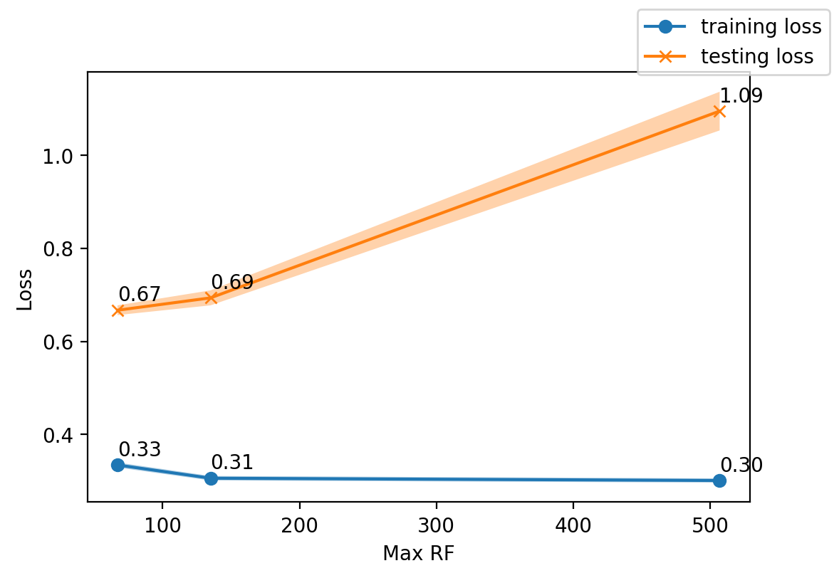
Figure 15: Comparing the training loss vs the testing loss of ResNets with the same number of parameters but with different Max RF. The difference in RF size is due to adding pooling layers. The increase of the testing loss with larger Max RF indicates overfitting. The CNNs are trained on DCASE‘18.

B-4 Skip and Residual Connections

Skip and residual connections are very common in modern architectures such as ResNet [8] and DenseNet [9]. Since we are studying the Max RF, if two branches are added or concatenated as an input for a layer, we consider the branch with the bigger Max RF when calculating the Max RF of the layer. Figure 16 shows the testing accuracy of variants of DenseNets with different growth rate. The growth rate determines the number of channels in the output of each Dense layer. This output is then presented as an input to all the following Dense layers, which is known as a Skip Connection. We show that all the variants degrade in performance in larger RF settings.

B-5 Dilated Convolution

A dilated convolutional layer [62] can be seen as a convolutional layer with a larger sparse filters which has the same number of learnable parameters. The effective filter size of dilated convolutional layer with $d_{n}$ dilation is $k_{n}^{*}=d_{n}(k_{n}-1)+1$. When $d=1$, $k_{n}^{*}=k_{n}$. However, when $d_{n}>1$, for receptive field calculation purposes, the dilated convolutional layer (with dilation $d_{n}$ and filter size $k_{n}$) can be seen as a regular convolutional with a larger filter $k_{n}^{*}$. Therefore, we can replace $k_{n}$ with $k_{n}^{*}$ in Equation 1 to calculate its receptive field.

In the case of $d_{n}>1$, although the activation of a spatial pixel of the output of a layer is affected by the same number of spatial pixels of the preceding layer as with $d=1$, two adjacent pixels cover a bigger number of pixels of the preceding layer.

Figure 16 shows the testing accuracy of a variants of CP_ResNet with dilated convolutional layers. We start the experiment with variants of CP_ResNet with a Max RF ranging from $55$ pixels to $199$ (corresponding $\rho$ from $3$ to $9$). We then change the convolution of different layers (in different experiments) to a dilated convolutional operator with $d=2$. We then calculate the Max RF and train the network and report the testing accuracy.

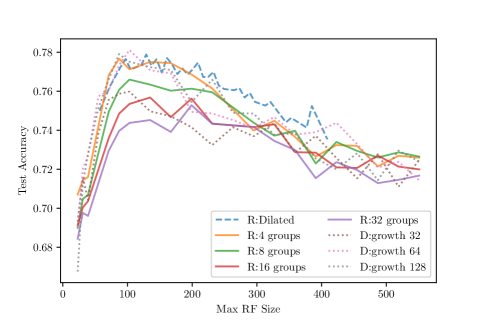
Figure 16: DCASE‘18 testing accuracy of different designs of CP_ResNet (R) and CP_DenseNet (D) convolutional layers.

B-6 Grouped Convolution

Grouped convolution restricts the receptive field of a layer over the channels dimension, and therefore does not impact the spatial RF of a CNN. This indicates that the same approach to control the Max RF can be applied to architectures that utilize grouped convolutional layers such as ResNext [57]. Figure 16 shows that the performance of variants of CP_ResNet with a different number of groups follows the same pattern.

B-7 Batch Normalization

Batch Normalization [63] in CNNs is calculated per channel. However, the mean and the variance are calculated across all the spatial pixels during training. During inference, the layer uses the training statistics and thus does not affect the Max RF.

B-8 Shake-Shake

Shake-Shake [64] regularization works by replacing the summation operation of residual branches by a stochastic affine combination. Gastaldi [64] shows empirically that using this regularization technique improves the generalization of a ResNet with two residual branches on various computer vision datasets. Gastaldi also shows that using different scaling coefficient for the residual branches in the backward pass improves the generalization. Previous work [15, 31] confirms that Shake-Shake regularization can boost performance on unseen data in some tasks as well, especially in the presence of noisy data or labels.

In Shake-Shake regularized architectures, both of the residual branches will have the same Max RF. Therefore, combining both with different scaling factors does not change the Max RF of the network. We apply Shake-Shake regularization to CP_ResNet in our experiments. The resulting network (SS CP_ResNet) will have consequently the same Max RF as explained in Section V-A1.

B-9 Frequency-Aware CNNs

Frequency-Aware CNNs [59] (FACNNs) showed empirically improvements in the performance of CNNs in acoustic scene classification [59], and emotion and theme detection [31] tasks. Frequency-aware convolutional layers work by concatenating a new channel to the input, that provides a positional encoding for the frequency. Unlike CNNs with restricted Max RF, CNNs with a large RF can infer the frequency positional information of their input. Hence, FACNNs were proposed to compensate for the lack of frequency-range information in CNNs with a restricted RF over the frequency dimension. Since adding the frequency information as a new channel does not affect the Max RF of the CNN, CP_ResNet with frequency-aware layers (CP_FAResNet) will have the same Max RF.

TABLE VII: Per-class accuracy Comparison of CP_ResNet with the state of the art on the DCASE‘19 Dataset

	Chen et al.[42]	CP_ResNet CV	Seo et al. [50]
Overall	85.2 %	83.7 %	82.5 %
Airport	77.5 %	79.9 %	74.9 %
Bus	96.1 %	96.2 %	95 %
Metro	89.9 %	84.7 %	82.9 %
Metro station	82.5 %	81.5 %	80 %
Park	96.7 %	96.1 %	92.4 %
Public square	67.5 %	64 %	60.7 %
Shopping mall	80 %	80.1 %	85.4 %
Street pedestrian	78.6 %	72.9 %	68.6 %
Street traffic	92.8 %	92.6 %	93.2 %
Tram	90.6 %	89 %	91.9 %

References

- [1] W. Liu, Z. Wang, X. Liu, N. Zeng, Y. Liu, and F. E. Alsaadi, “A survey of deep neural network architectures and their applications,” Neurocomputing, vol. 234, pp. 11 – 26, 2017.
- [2] A. Krizhevsky, I. Sutskever, and G. E. Hinton, “Imagenet classification with deep convolutional neural networks,” in Advances in Neural Information Processing Systems, 2012, pp. 1097–1105.
- [3] Y. Shen, X. He, J. Gao, L. Deng, and G. Mesnil, “Learning semantic representations using convolutional neural networks for web search,” in Proceedings of the 23rd International Conference on World Wide Web, 2014, pp. 373–374.
- [4] Y. Kim, “Convolutional neural networks for sentence classification,” in Proceedings of the 2014 Conference on Empirical Methods in Natural Language Processing (EMNLP), Doha, Qatar, Oct. 2014, pp. 1746–1751.
- [5] R. Collobert and J. Weston, “A unified architecture for natural language processing: Deep neural networks with multitask learning,” in Proceedings of the International Conference on Machine Learning, 2008, p. 160–167.
- [6] G. Hinton, L. Deng, D. Yu, G. E. Dahl, A. Mohamed, N. Jaitly, A. Senior, V. Vanhoucke, P. Nguyen, T. N. Sainath, and B. Kingsbury, “Deep neural networks for acoustic modeling in speech recognition: The shared views of four research groups,” IEEE Signal Processing Magazine, vol. 29, no. 6, pp. 82–97, Nov 2012.
- [7] K. Simonyan and A. Zisserman, “Very deep convolutional networks for large-scale image recognition,” in 3rd International Conference on Learning Representations, ICLR 2015, 2015.
- [8] K. He, X. Zhang, S. Ren, and J. Sun, “Deep residual learning for image recognition,” in IEEE Conference On Computer Vision and Pattern Recognition, pp. 770–778.
- [9] G. Huang, Z. Liu, L. Van Der Maaten, and K. Q. Weinberger, “Densely connected convolutional networks,” in IEEE Conference On Computer Vision and Pattern Recognition, pp. 4700–4708.
- [10] H. Lee, R. B. Grosse, R. Ranganath, and A. Y. Ng, “Convolutional deep belief networks for scalable unsupervised learning of hierarchical representations,” in Proceedings of the International Conference on Machine Learning, vol. 382, 2009, pp. 609–616.
- [11] H. Eghbal-zadeh, B. Lehner, M. Dorfer, and G. Widmer, “CP-JKU submissions for DCASE-2016: A hybrid approach using binaural i-vectors and deep convolutional neural networks,” DCASE2016 Challenge, Tech. Rep.
- [12] S. Hershey, S. Chaudhuri, D. P. W. Ellis, J. F. Gemmeke, A. Jansen, R. C. Moore, M. Plakal, D. Platt, R. A. Saurous, B. Seybold, M. Slaney, R. J. Weiss, and K. Wilson, “CNN architectures for large-scale audio classification,” in IEEE International Conference on Acoustics, Speech and Signal Processing (ICASSP), pp. 131–135.
- [13] W. Luo, Y. Li, R. Urtasun, and R. Zemel, “Understanding the Effective Receptive Field in Deep Convolutional Neural Networks,” in Advances in Neural Information Processing Systems, 2016, pp. 4898–4906.
- [14] P. Primus, H. Eghbal-zadeh, D. Eitelsebner, K. Koutini, A. Arzt, and G. Widmer, “Exploiting parallel audio recordings to enforce device invariance in CNN-based acoustic scene classification,” in Proceedings of the Detection and Classification of Acoustic Scenes and Events 2019 Workshop (DCASE2019), NY, USA, October 2019, pp. 204–208.
- [15] K. Koutini, H. Eghbal-zadeh, and G. Widmer, “CP-JKU submissions to DCASE’19: Acoustic scene classification and audio tagging with receptive-field-regularized CNNs,” DCASE2019 Challenge, Tech. Rep., June 2019.
- [16] S. Suh, S. Park, Y. Jeong, and T. Lee, “Designing Acoustic Scene Classification Models with CNN Variants,” DCASE2020 Challenge, Tech. Rep., 2020.
- [17] K. Koutini, F. Henkel, H. Eghbal-zadeh, and G. Widmer, “CP-JKU Submissions to Dcase’20: Low-Complexity Cross-Device Acoustic Scene Classification with RF-Regularized CNNs,” DCASE2020 Challenge, Tech. Rep., 2020.
- [18] E. Fonseca, M. Plakal, F. Font, D. P. Ellis, and X. Serra, “Audio tagging with noisy labels and minimal supervision,” in Proceedings of the Detection and Classification of Acoustic Scenes and Events 2019 Workshop (DCASE2019), NY, USA, October 2019, pp. 69–73.
- [19] B. Lehner and K. Koutini, “Acoustic scene classification with reject option based on ResNets,” DCASE2019 Challenge, Tech. Rep., June 2019.
- [20] B. Lehner, H. Eghbal-Zadeh, M. Dorfer, F. Korzeniowski, K. Koutini, and G. Widmer, “Classifying short acoustic scenes with I-vectors and CNNs: Challenges and optimisations for the 2017 DCASE ASC task.” DCASE2017 Challenge.
- [21] M. Dorfer, B. Lehner, H. Eghbal-zadeh, C. Heindl, F. Paischer, and G. Widmer, “Acoustic Scene Classification with Fully Convolutional Neural Networks and I-Vectors,” DCASE2018 Challenge, Tech. Rep.
- [22] Y. Sakashita and M. Aono, “Acoustic Scene Classification by Ensemble of Spectrograms Based on Adaptive Temporal Divisions,” DCASE2018 Challenge, Tech. Rep.
- [23] S. Zhao, T. N. T. Nguyen, W.-S. Gan, and J. Douglas L., “ADSC submission for DCASE 2017: Acoustic scene classification using deep residual convolutional neural networks,” DCASE2017 Challenge, Tech. Rep.
- [24] A. Mesaros, T. Heittola, A. Diment, B. Elizalde, A. Shah, E. Vincent, B. Raj, and T. Virtanen, “DCASE 2017 challenge setup: Tasks, datasets and baseline system,” in Proceedings of the Detection and Classification of Acoustic Scenes and Events 2017 Workshop (DCASE2017), 2017.
- [25] M. A. Carlin and M. Elhilali, “A framework for speech activity detection using adaptive auditory receptive fields,” IEEE/ACM Transactions on audio, speech, and language processing, vol. 23, pp. 2422–2433, 2015.
- [26] J. B. Fritz, M. Elhilali, S. V. David, and S. A. Shamma, “Auditory attention—focusing the searchlight on sound,” Current opinion in neurobiology, vol. 17, no. 4, pp. 437–455, 2007.
- [27] V. M. Bajo and A. J. King, “Focusing attention on sound,” Nature neuroscience, vol. 13, no. 8, pp. 913–914, 2010.
- [28] S. Shamma and J. Fritz, “Adaptive auditory computations,” Current opinion in neurobiology, vol. 25, pp. 164–168, 2014.
- [29] J. Pons, T. Lidy, and X. Serra, “Experimenting with musically motivated convolutional neural networks,” in 2016 14th International Workshop on Content-Based Multimedia Indexing (CBMI), pp. 1–6.
- [30] D. Bogdanov, M. Won, P. Tovstogan, A. Porter, and X. Serra, “The MTG-Jamendo dataset for automatic music tagging,” in Machine Learning for Music Discovery Workshop, (ICML 2019)., 2019.
- [31] K. Koutini, S. Chowdhury, V. Haunschmid, H. Eghbal-Zadeh, and G. Widmer, “Emotion and theme recognition in music with Frequency-Aware RF-Regularized CNNs,” in Working Notes Proceedings of the MediaEval 2019 Workshop. ceur-ws.org, 12 2019.
- [32] M. Sukhavasi and S. Adapa, “Music theme recognition using cnn and self-attention,” in Working Notes Proceedings of the MediaEval 2019 Workshop. ceur-ws.org, 12 2019.
- [33] S. Amiriparian, M. Gerczuk, E. Coutinho, A. Baird, S. Ottl, M. Milling, and B. Schuller, “Emotion and themes recognition in music utilising convolutional and recurrent neural networks,” in Working Notes Proceedings of the MediaEval 2019 Workshop. ceur-ws.org, 12 2019.
- [34] M. Sandler, A. Howard, M. Zhu, A. Zhmoginov, and L.-C. Chen, “Mobilenetv2: Inverted residuals and linear bottlenecks,” in Proceedings of the IEEE conference on computer vision and pattern recognition, 2018, pp. 4510–4520.
- [35] A. Vaswani, N. Shazeer, N. Parmar, J. Uszkoreit, L. Jones, A. N. Gomez, Ł. Kaiser, and I. Polosukhin, “Attention is all you need,” in Advances in Neural Information Processing Systems, 2017, pp. 5998–6008.
- [36] J. F. Gemmeke, D. P. W. Ellis, D. Freedman, A. Jansen, W. Lawrence, R. C. Moore, M. Plakal, and M. Ritter, “Audio set: An ontology and human-labeled dataset for audio events,” in IEEE International Conference on Acoustics, Speech and Signal Processing (ICASSP), New Orleans, LA, 2017.
- [37] J. Deng, W. Dong, R. Socher, L.-J. Li, K. Li, and L. Fei-Fei, “Imagenet: A large-scale hierarchical image database,” in IEEE Conference On Computer Vision and Pattern Recognition., pp. 248–255.
- [38] E. Humphrey, S. Durand, and B. McFee, “Openmic-2018: An open data-set for multiple instrument recognition,” in Proceedings of the 19th International Society for Music Information Retrieval Conference, ISMIR 2018, Paris, France, September 23-27, 2018, 2018, pp. 438–444.
- [39] S. Gururani, M. Sharma, and A. Lerch, “An attention mechanism for musical instrument recognition,” in Proceedings of the 20th International Society for Music Information Retrieval Conference, ISMIR 2019, Delft, The Netherlands, November 4-8, 2019, 2019, pp. 83–90.
- [40] A. Kenarsari-Anhari, “Learning multi-instrument classification with partial labels,” CoRR, vol. abs/2001.08864, 2020.
- [41] S. Hochreiter and J. Schmidhuber, “Long short-term memory,” Neural Computation, vol. 9, no. 8, pp. 1735–1780, 1997.
- [42] H. Chen, Z. Liu, Z. Liu, P. Zhang, and Y. Yan, “Integrating the data augmentation scheme with various classifiers for acoustic scene modeling,” DCASE2019 Challenge, Tech. Rep., June 2019.
- [43] A. Mesaros, T. Heittola, and T. Virtanen, “A multi-device dataset for urban acoustic scene classification,” in Proceedings of the Detection and Classification of Acoustic Scenes and Events 2018 Workshop (DCASE2018), pp. 9–13.
- [44] ——, “Acoustic scene classification in DCASE 2019 challenge: Closed and open set classification and data mismatch setups,” in Proceedings of the Detection and Classification of Acoustic Scenes and Events 2019 Workshop (DCASE2019), NY, USA, October 2019, pp. 164–168.
- [45] V. Lostanlen, J. Andén, and M. Lagrange, “Extended playing techniques: The next milestone in musical instrument recognition,” in Proceedings of the 5th International Conference on Digital Libraries for Musicology, ser. DLfM ’18. New York, NY, USA: Association for Computing Machinery, 2018, p. 1–10.
- [46] S. Gururani, C. Summers, and A. Lerch, “Instrument activity detection in polyphonic music using deep neural networks,” in Proceedings of the 19th International Society for Music Information Retrieval Conference, ISMIR 2018, Paris, France, September 23-27, 2018, E. Gómez, X. Hu, E. Humphrey, and E. Benetos, Eds., 2018, pp. 569–576.
- [47] Y. Han, S. Lee, J. Nam, and K. Lee, “Sparse feature learning for instrument identification: Effects of sampling and pooling methods,” The Journal of the Acoustical Society of America, vol. 139, no. 5, pp. 2290–2298, 2016.
- [48] M. Defferrard, K. Benzi, P. Vandergheynst, and X. Bresson, “FMA: A dataset for music analysis,” in Proceedings of the 18th International Society for Music Information Retrieval Conference, ISMIR 2017, Suzhou, China, October 23-27, 2017, 2017, pp. 316–323.
- [49] K. He, X. Zhang, S. Ren, and J. Sun, “Identity mappings in deep residual networks,” arXiv preprint arXiv:1603.05027, 2016.
- [50] S. Hyeji and P. Jihwan, “Acoustic scene classification using various pre-processed features and convolutional neural networks,” DCASE2019 Challenge, Tech. Rep., June 2019.
- [51] A. Odena, C. Olah, and J. Shlens, “Conditional image synthesis with auxiliary classifier gans,” in Proceedings of the International Conference on Machine Learning, ICML, vol. 70, 2017, pp. 2642–2651.
- [52] K. Sohn, H. Lee, and X. Yan, “Learning structured output representation using deep conditional generative models,” in Advances in Neural Information Processing Systems, 2015, pp. 3483–3491.
- [53] K. Koutini, H. Eghbal-zadeh, M. Dorfer, and G. Widmer, “The Receptive Field as a Regularizer in Deep Convolutional Neural Networks for Acoustic Scene Classification,” in Proceedings of the European Signal Processing Conference (EUSIPCO), A Coruña, Spain, 2019.
- [54] G. Castel-Branco, G. Falcao, and F. Perdigão, “Enhancing the Labelling of Audio Samples for Automatic Instrument Classification Based on Neural Networks,” in IEEE International Conference on Acoustics, Speech and Signal Processing (ICASSP), 2020, pp. 1583–1587.
- [55] M. Tan and Q. V. Le, “EfficientNet: Rethinking model scaling for convolutional neural networks,” in Proceedings of the International Conference on Machine Learning, 2019, pp. 6105–6114.
- [56] P. Nakkiran, G. Kaplun, Y. Bansal, T. Yang, B. Barak, and I. Sutskever, “Deep double descent: Where bigger models and more data hurt,” in 8th International Conference on Learning Representations, ICLR 2020, Addis Ababa, Ethiopia, April 26-30, 2020, 2020.
- [57] S. Xie, R. Girshick, P. Dollár, Z. Tu, and K. He, “Aggregated residual transformations for deep neural networks,” in IEEE Conference On Computer Vision and Pattern Recognition, 2017, pp. 1492–1500.
- [58] H. Zhang, M. Cissé, Y. N. Dauphin, and D. Lopez-Paz, “mixup: Beyond empirical risk minimization,” in 6th International Conference on Learning Representations, ICLR 2018, Vancouver, BC, Canada, April 30 - May 3, 2018, Conference Track Proceedings, 2018.
- [59] K. Koutini, H. Eghbal-zadeh, and G. Widmer, “Receptive-field-regularized CNN variants for acoustic scene classification,” in Proceedings of the Detection and Classification of Acoustic Scenes and Events 2019 Workshop (DCASE2019), NY, USA, October 2019.
- [60] D. P. Kingma and J. Ba, “Adam: A method for stochastic optimization,” in 3rd International Conference on Learning Representations, ICLR 2015, San Diego, CA, USA, May 7-9, 2015, Conference Track Proceedings, Y. Bengio and Y. LeCun, Eds., 2015.
- [61] A. Araujo, W. Norris, and J. Sim, “Computing receptive fields of convolutional neural networks,” Distill, 2019, https://distill.pub/2019/computing-receptive-fields.
- [62] F. Yu and V. Koltun, “Multi-scale context aggregation by dilated convolutions,” in 4th International Conference on Learning Representations, ICLR 2016, San Juan, Puerto Rico, May 2-4, 2016, Conference Track Proceedings, Y. Bengio and Y. LeCun, Eds., 2016.
- [63] S. Ioffe and C. Szegedy, “Batch normalization: Accelerating deep network training by reducing internal covariate shift,” in Proceedings of the International Conference on Machine Learning, 2015, pp. 448–456.
- [64] X. Gastaldi, “Shake-shake regularization of 3-branch residual networks,” in International Conference on Learning Representations, Workshop Track Proceedings, 2017.