The Farey Sequence and the Mertens Function

Abstract

Franel and Landau derived an arithmetic statement involving the Farey sequence that is equivalent to the Riemann hypothesis. Since there is a relationship between the Mertens function and the Riemann hypothesis, there should be a relationship between the Mertens function and the Farey sequence. Functions of subsets of the fractions in Farey sequences that are analogous to the Mertens function are introduced. Mikolás proved that the sum of certain Mertens function values is 1. Results analogous to Mikolás’ theorem are the defining property of these functions. A relationship between the Farey sequence and the Riemann hypothesis other than the Franel-Landau theorem is postulated. This conjecture involves a theorem of Mertens and the second Chebyshev function.

1 Introduction

Mikolás [1] proved that $\sum_{n=1}^{x}M(\lfloor x/n\rfloor)=1$ where $M$ denotes the Mertens function. If $f$ and $g$ are two arithmetical function, their Dirichlet product (or convolution) is defined by the equation $h(n)=\sum_{d|n}f(d)g(n/d)$ (denoted by $f*g$ for $h$ and $(f*g)(n)$ for $h(n)$). Let $F$ denote a real or complex-valued function defined on the positive real axis (0, +$\infty$) such that $F(x)=0$ for $0<x<1$. A more general convolution is $\sum_{n\leq x}\alpha(n)F(x/n)$ where $\alpha$ is any arithmetical function. The sum defines a new function $G$ on $(0,+\infty)$ which also vanishes for $0<x<1$. The function $G$ is denoted by $\alpha\circ F$. An associative property relating $\circ$ and $*$ is given by Lemma 1.

Lemma 1

For any arithmetical function $\alpha$ and $\beta$, $\alpha\circ(\beta\circ F)=(\alpha*\beta)\circ F$.

(See section 2.14 of Apostol’s [2] book.) The functions considered here are $\alpha(n)=1$, $b(n)=\lfloor n/2\rfloor-2\lfloor n/4\rfloor$ and $F(n)=M(n)$. The Farey sequence of order $n$ (denoted by $\mathcal{F}_{n})$ is the ascending sequence of irreducible fractions between 0 and 1 whose denominators do not exceed $n$. Corollary 1.33 in Matveev’s [3] book is given by Lemma 2

Lemma 2

If $f_{t}\in\mathcal{F}_{n}-\{1/1\}$ where $n>1$, then $t=\sum_{j=2}^{n}M(n/j)\lfloor jf_{t}\rfloor$ where $M(\cdot)$ is the Mertens function.

Previously, Mikolás proved a slightly more general version of this. Let $\varrho_{\nu}$ denote the $\nu$-th fraction in $F_{x}$ (the Farey sequence of order $x$) and $\mu(n)$ the Möbius function. Mikolás’ Lemma 4 is given by Lemma 3.

Lemma 3

Let $0\leq\xi\leq 1$ and let us denote by $h(\xi,x)$ the number of fractions in $F_{x}$ which are not greater than $\xi$. Then we have $h(\xi,x)=\sum_{\varrho_{\nu}\leq\xi}1=\sum_{n=1}^{[x]}[n\xi]M(\frac{x}{n})=\sum_{n=1}^{[x]}\mu(n)\sum_{d=1}^{[x/n]}[d\xi]$.

$\beta\circ M$ is then the difference between the number of fractions less than or equal to 1/2 and greater than 1/4 and the number of fractions less than or equal to 1/4.

2 The Farey Sequence and Redheffer matrices

Mikolás proved that $\sum_{i=1}^{x}M(\lfloor x/i\rfloor)=1$. In general, $\sum_{i=1}^{x}M(\lfloor x/(in)\rfloor)=1$, $n=1,2,3,\ldots,x$ (since $\lfloor\lfloor x/n\rfloor/i\rfloor=\lfloor x/(in)\rfloor$). Let $R^{\prime}$ denote a square matrix where element $(i,j)$ equals 1 if $j$ divides $i$ or 0 otherwise. In a Redheffer matrix, element $(i,j)$ equals 1 if $i$ divides $j$ or if $j=1$. Redheffer [4] proved that the determinant of such a $x$ by $x$ matrix equals $M(x)$. Let $T$ denote the matrix obtained from $R^{\prime}$ by element-by-element multiplication of the columns by $M(\lfloor x/1\rfloor),M(\lfloor x/2\rfloor),M(\lfloor x/3\rfloor),\ldots,M(\lfloor x/x\rfloor)$. For example, the $T$ matrix for $x=12$ is

$-2$	0	0	0	0	0	0	0	0	0	0	0
$-1$	$-1$	0	0	0	0	0	0	0	0	0	0
$-1$	0	$-1$	0	0	0	0	0	0	0	0	0
$-1$	$-1$	0	$-1$	0	0	0	0	0	0	0	0
0	0	0	0	0	0	0	0	0	0	0	0
0	0	0	0	0	0	0	0	0	0	0	0
1	0	0	0	0	0	1	0	0	0	0	0
1	1	0	1	0	0	0	1	0	0	0	0
1	0	1	0	0	0	0	0	1	0	0	0
1	1	0	0	1	0	0	0	0	1	0	0
1	0	0	0	0	0	0	0	0	0	1	0
1	1	1	1	0	1	0	0	0	0	0	1

Let $\Phi(x)$ denote $\sum_{i=1}^{x}\varphi(i)$ where $\varphi$ is Euler’s totient function. This is also the number of fractions in a Farey sequence of order $x$. Let $U$ denote the matrix obtained from $T$ by element-by-element multiplication of the columns by $\varphi(j)$. The sum of the sums of the columns of $U$ then equals $\Phi(x)$. $i=\sum_{d|i}\varphi(d)$, so $\sum_{i=1}^{x}M(\lfloor x/i\rfloor)i$ (the sum of the sums of the rows of $U$) equals $\Phi(x)$. This relationship given by equation 1 was proved by Cox [5].

$$\sum_{i=1}^{x}M(\lfloor x/i\rfloor)i=\Phi(x)$$ (1)

Previously, Mikolás proved this using a different approach. Let $f(n)$ and $g(n)$ be arbitrary arithmetical functions. Mikolás Lemma 2 is given by equation 2.

$$\sum_{n=1}^{[x]}\sum_{d|n}f(d)g(\frac{n}{d})=\sum_{d=1}^{[x]}f(d)\sum_{\delta=1}^{[x/d]}g(\delta)=\sum_{d=1}^{[x]}g(d)\sum_{\delta=1}^{[x/d]}f(\delta)$$ (2)

Special cases of this are given by equation 3.

$$\sum_{n=1}^{[x]}\sum_{d|n}f(d)=\sum_{d=1}^{[x]}[\frac{x}{d}]f(d)=\sum_{d=1}^{[x]}\sum_{\delta=1}^{[x/d]}f(\delta)$$ (3)

From this, Mikolás determined that equations 4 and 5 hold.

$$\sum_{n=1}^{[x]}M(\frac{x}{n})=\sum_{n=1}^{[x]}\mu(n)[\frac{x}{n}]=1$$ (4)

$$\Phi(x)=\sum_{n=1}^{[x]}\varphi(n)=\sum_{n=1}^{[x]}nM(\frac{x}{n})=\frac{1}{2}\sum_{n=1}^{[x]}\mu(n)[\frac{x}{n}]^{2}+\frac{1}{2}$$ (5)

Let $\sigma_{x}(i)$ denote the sum of positive divisors function ($\sigma_{x}(i)=\sum_{d|i}d^{x}$). Another relationship proved by Cox is given by Lemma 4.

Lemma 4

$\sum_{i=1}^{x}M(\lfloor x/i\rfloor)\sigma_{0}(i)=x$

The right-hand side of the equation is simply the number of columns in the above modified Redheffer matrix. The sum of each column is 1 and the respective sums of the rows are $M(\lfloor x/1\rfloor)\sigma_{0}(1)$, $M(\lfloor x/2\rfloor)\sigma_{0}(2)$, $M(\lfloor x/3\rfloor)\sigma_{0}(3)$,$\ldots$,$M(\lfloor x/x\rfloor)\sigma_{0}(x)$.

3 Properties of $1*\beta$

A result from the literature (see 2.11 of Tenenbaum’s [6] book) is given by Lemma 5.

Lemma 5

$1*1=\sigma_{0}$

A more general result from the literature (see 2.7 of Tenenbaum’s book) is given by Lemma 6.

Lemma 6

$(1*f)(n)=\sum_{d|n}f(d)$

Note that $\lfloor j/2\rfloor-2\lfloor j/4\rfloor$ equals $\lfloor(j+4)/2\rfloor-2\lfloor(j+4)/4\rfloor$. The values of $\lfloor j/2\rfloor-2\lfloor j/4\rfloor$ for $j=1,2,3,\ldots$ are then $0,1,1,0,0,1,1,0,0,1,1,0\ldots$. The values depend on whether $j$ is of the form $4k$, $4k+1$, $4k+2$, or $4k+3$. Let $f_{1}(d)=1$ if $d=4k$, $f_{2}(d)=1$ if $d=4k+1$, $f_{3}(d)=1$ if $d=4k+2$, and $f_{4}(d)=1$ if $d=4k+3$. Then by Lemma 4, Lemma 5, and Lemma 6, there are four “lines” with a slope of $\frac{1}{4}$ (out of phase by one position) corresponding to the convolution of these functions with the Mertens function. A plot of these “lines” is given in Figure 1.

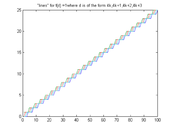
Figure 1: Plot of lines resulting from convolution with Mertens function

Note that two of the above “lines” can be added to give a “line” with a slope of $\frac{1}{2}$, three can be added to give a “line” with a slope of $\frac{3}{4}$, or all of them can be added to give a straight line with a slope of 1.

Let $m_{x}$ denote the number of fractions up to and including $\frac{1}{4}$ and $n_{x}$ the number of fractions after $\frac{1}{4}$ and up to and including $\frac{1}{2}$ in a Farey sequence of order $x$ ($m_{1}$, $m_{2}$, $n_{1}$ and $n_{2}$ are set to 0). A consequence of the above convolution is given by Corollary 1.

Corollary 1

$\sum_{i=1}^{x}(n_{\lfloor x/i\rfloor}-m_{\lfloor x/i\rfloor}+\frac{1}{4})$ equals $\frac{1}{2}$, $\frac{1}{4}$, $0$, or $-\frac{1}{4}$

4 Farey Sequences and the Riemann Hypothesis

For $\nu=1,2,3,\ldots,\Phi(x)$ let $\delta_{\nu}$ denote the amount by which the $\nu$-th term of the Farey sequence differs from $\nu/\Phi(x)$. The theorem of Franel and Landau [7] is that the Riemann hypothesis is equivalent to the statement that $|\delta_{1}|+|\delta_{2}|+|\delta_{3}|+,\ldots,+|\delta_{\Phi(x)}|=o(x^{1/2+\epsilon})$ for all $\epsilon>0$ as $x\rightarrow\infty$.

Let $\Lambda(i)$ denote the Mangoldt function ($\Lambda(i)$ equals $\log(p)$ if $i=p^{m}$ for some prime $p$ and some $m\geq 1$ or $0$ otherwise). Let $\psi(x)$ denote the second Chebyshev function ($\psi(x)=\sum_{i\leq x}\Lambda(i)$). Mertens [8] proved that equation 6 holds.

$$\sum_{i=1}^{x}M(\lfloor x/i\rfloor)\log(i)=\psi(x)$$ (6)

A plot of $\psi(x)$ and $\sum_{i=1}^{x}(m_{\lfloor x/i\rfloor}-n_{\lfloor x/i\rfloor}+\frac{1}{4})\log(i)$ for $x=2,3,4,\ldots,10000$ is given in Figure 2.

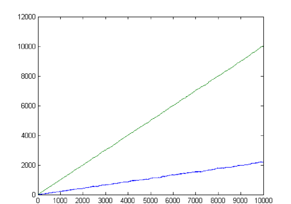
Figure 2: Plot of the second Chebyshev function and corresponding sums

The slope of $\sum_{i=1}^{x}(m_{\lfloor x/i\rfloor}-n_{\lfloor x/i\rfloor}+\frac{1}{4})\log(i)$ is approximately 0.2197 whereas the slope of $\psi(x)$ is approximately 1.0.

The Riemann hypothesis is equivalent to the arithmetic statement $\psi(x)-x=o(x^{1/2+\epsilon})$ for all $\epsilon>0$. For a linear least-squares fit of $\psi(x)$ for $x=2,3,4,\ldots,10000$, $p_{1}=1$ with a 95% confidence interval of (1, 1), $p_{2}=-2.122$ with a 95% confidence interval of ($-2.699$, $-1.545$), SSE=$2.165\cdot 10^{6}$, R-squared=1, and RMSE=14.72. For a linear least-squares fit of $\sum_{i=1}^{x}(m_{\lfloor x/i\rfloor}-n_{\lfloor x/i\rfloor}+\frac{1}{4})\log(i)$ for $x=2,3,4,\ldots,10000$, $p_{1}=0.2197$ with a 95% confidence interval of (0.2196, 0.2198), $p_{2}=-1.246$ with a 95% confidence interval of ($-1.841$, $-0.6504$), SSE=$2.303\cdot 10^{6}$, R-squared=0.9994, and RMSE=15.18. For a linear least-squares fit of $\psi(x)$ for $x=2,3,4,\ldots,25000$, $p_{1}=1$ with a 95% confidence interval of (1, 1), $p_{2}=-5.18$ with a 95% confidence interval of ($-5.821$, $-4.54$), SSE=$1.667\cdot 10^{7}$, R-squared=1, and RMSE=25.82. For a linear least-squares fit of $\sum_{i=1}^{x}(m_{\lfloor x/i\rfloor}-n_{\lfloor x/i\rfloor}+\frac{1}{4})\log(i)$ for $x=2,3,4,\ldots,25000$, $p_{1}=0.2197$ with a 95% confidence interval of (0.2197, 0.2198), $p_{2}=-2.773$ with a 95% confidence interval of ($-3.358$, $-2.189$), SSE=$1.388\cdot 10^{7}$, R-squared=0.9998, and RMSE=23.56. The sum-squared errors (SSE) and root-mean-squared errors (RMSE) are approximately equal. This is the basis for the following Conjecture 1.

Conjecture 1

The Riemann hypothesis is equivalent to the arithmetic statement $\sum_{i=1}^{x}(m_{\lfloor x/i\rfloor}-n_{\lfloor x/i\rfloor}+\frac{1}{4})\log(i)-0.2197x=o(x^{1/2+\epsilon})$ for all $\epsilon>0$.

5 Infinitely Many Analogues of the Mertens Function

Let $o_{x}$ denote the number of fractions up to and including $\frac{1}{5}$ and $p_{x}$ the number of fractions after $\frac{1}{5}$ and up to and including $\frac{2}{5}$ in a Farey sequence of order $x$. Let $q_{x}$ denote the number of fractions up to including $\frac{1}{6}$ and $r_{x}$ the number of fractions after $\frac{1}{6}$ and up to and including $\frac{1}{3}$ in a Farey sequence of order $x$. Let $s_{x}$ denote the number of fractions up to and including $\frac{1}{7}$ and $t_{x}$ the number of fractions after $\frac{1}{7}$ and up to and including $\frac{2}{7}$ in a Farey sequence of order $x$. Let $u_{x}$ denote the number of fractions up to and including $\frac{1}{8}$ and $v_{x}$ the number of fractions after $\frac{1}{8}$ and up to and including $\frac{1}{4}$ in a Farey sequence of order $x$. The following corollaries can be proved by using Lemma 1, Lemma 2, Lemma 4, Lemma 5, and Lemma 6 just as they were used to prove Corollary 1.

Corollary 2

$\sum_{i=1}^{x}(o_{\lfloor x/i\rfloor}-p_{\lfloor x/i\rfloor}+\frac{2}{5})$ equals $\frac{4}{5}$, $\frac{1}{5}$, $0$, $-\frac{1}{5}$, or $-\frac{2}{5}$

For a linear least-squares fit of $\sum_{i=1}^{x}(o_{\lfloor x/i\rfloor}-p_{\lfloor x/i\rfloor}+\frac{2}{5})\log(i)$ for $x=2,3,4,\ldots,25000$, $p_{1}=0.3733$ with a 95% confidence interval of (0.3733, 0.3734), $p_{2}=1.598$ with a 95% confidence interval of (0.9739, 2.222), SSE=$1.583\cdot 10^{7}$, R-squared=0.9999, and RMSE=25.17.

Corollary 3

$\sum_{i=1}^{x}(q_{\lfloor x/i\rfloor}-r_{\lfloor x/i\rfloor}+\frac{1}{3})$ equals $1$, $\frac{2}{3}$, $\frac{1}{3}$, $0$, or $-\frac{1}{3}$

For a linear least-squares fit of $\sum_{i=1}^{x}(q_{\lfloor x/i\rfloor}-r_{\lfloor x/i\rfloor}+\frac{1}{3})\log(i)$ for $x=2,3,4,\ldots,25000$, $p_{1}=0.4218$ with a 95% confidence interval of (0.4218, 0.4218), $p_{2}=-2.837$ with a 95% confidence interval of ($-3.449$, $-2.225$), SSE=$1.523\cdot 10^{7}$, R-squared=0.9999, and RMSE=24.69.

Corollary 4

$\sum_{i=1}^{x}(s_{\lfloor x/i\rfloor}-t_{\lfloor x/i\rfloor}+\frac{3}{7})$ equals $\frac{9}{7}$, $\frac{6}{7}$, $\frac{5}{7}$, $\frac{3}{7}$, $\frac{1}{7}$, $0$, or $-\frac{3}{7}$

For a linear least-squares fit of $\sum_{i=1}^{x}(s_{\lfloor x/i\rfloor}-t_{\lfloor x/i\rfloor}+\frac{3}{7})\log(i)$ for $x=2,3,4,\ldots,25000$, $p_{1}=0.5572$ with a 95% confidence interval of (0.5572, 0.5573), $p_{2}=-1.185$ with a 95% confidence interval of ($-1.87$, $-0.5011$), SSE=$1.904\cdot 10^{7}$, R-squared=1, and RMSE=27.6.

Corollary 5

$\sum_{i=1}^{x}(u_{\lfloor x/i\rfloor}-v_{\lfloor x/i\rfloor}+\frac{3}{8})$ equals $\frac{9}{8}$, $\frac{3}{2}$, $\frac{7}{8}$, $\frac{3}{4}$, $\frac{3}{8}$, $\frac{1}{4}$, $0$, or $-\frac{3}{8}$

For a linear least-squares fit of $\sum_{i=1}^{x}(u_{\lfloor x/i\rfloor}-v_{\lfloor x/i\rfloor}+\frac{3}{8})\log(i)$ for $x=2,3,4,\ldots,25000$, $p_{1}=0.5782$ with a 95% confidence interval of (0.5782, 0.5783), $p_{2}=0.9218$ with a 95% confidence interval of ($0.2422$, $1.601$), SSE=$1.878\cdot 10^{7}$, R-squared=1, and RMSE=27.41.

In general, the differences between the number of fractions up to and including $1/I$ and after $1/I$ and up to and including $2/I$, $I=4,5,6,\ldots$ are incremented by $\frac{\lfloor(I+1)/2\rfloor-1}{I}$. For $I=4$, $\lfloor j/2\rfloor-2\lfloor j/4\rfloor$ equals $\lfloor(j+4)/2\rfloor-2\lfloor(j+4)/4\rfloor$. For $I>4$, similar expressions determine the periods and thus the slopes of the “lines” and the increments required to compensate for the slopes.

A plot of these and subsequent slopes at even $I$ values is given in Figure 3.

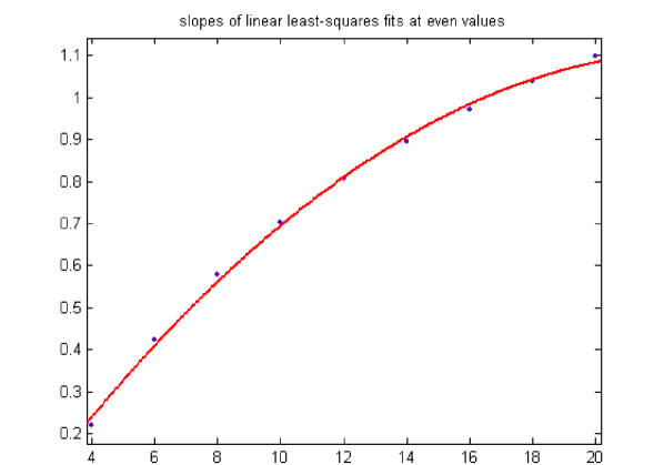
Figure 3: Plot of the slopes of linear least-squares fits at even I values

For a quadratic least-squares fit of the data, R-squared=0.998. A plot of the slopes at corresponding odd $I$ values is given in Figure 4.

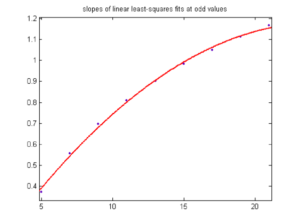
Figure 4: Plot of the slopes of linear least-squares fits at odd I values

For a quadratic least-squares fit of the data, R-squared=0.9978.

6 Conclusion

The above analogues of the Mertens function can be substituted for the Mertens function in many equations and the results analyzed. No method for proving the conjecture has been determined.

References

- [1] M. Mikolás, Farey series and their connection with the prime number problem 1, Acta Sci. Math. (Szeged) 13 (1949), 93-117
- [2] T. M. Apostol, Introduction to Analytic Number Theory, Springer, (1976)
- [3] A. O. Matveev, Farey Sequences: Duality and Maps Between Subsequences, De Gruyter, (2017)
- [4] R. M. Redheffer, Eine explizit lösbare Optimierungsaufgabe, Internat. Schriftenreine Numer. Math., 36 (1977)
- [5] Cox, Darrell and Ghosh, Sourangshu and Sultanow, Eldar. (2021). Bounds of the Mertens Functions. Advances in Dynamical Systems and Applications. 16. 35-44
- [6] Gérald Tenenbaum, Introduction to Analytic and Probabilistic Number Theory: Third Edition, American Mathematical Society, (2015)
- [7] Franel, J., and Landau, E., Les suites de Farey et le probleme des nombres premiers. Göttinger Nachr., 198-206 (1924)
- [8] F. Mertens, Über eine zahlentheoretische Funktion, Akademie Wissenschaftlicher Wien Mathematik-Naturlich Kleine Sitzungsber, 106 (1897) 761-830