Atom-in-jellium predictions of the shear modulus at high pressure

Abstract

Atom-in-jellium calculations of the Einstein frequency in condensed matter and of the equation of state were used to predict the variation of shear modulus from zero pressure to $\sim 10^{7}$ g/cm³, for several elements relevant to white dwarf (WD) stars and other self-gravitating systems. This is by far the widest range reported electronic structure calculation of shear modulus, spanning from ambient through the one-component plasma to extreme relativistic conditions. The predictions were based on a relationship between Debye temperature and shear modulus which we assess to be accurate at the $o(10\%)$ level, and is the first known use of atom-in-jellium theory to calculate a shear modulus. We assessed the overall accuracy of the method by comparing with experimental measurements and more detailed electronic structure calculations at lower pressures.

I Introduction

The shear modulus is a fundamental measure of the resistance of matter to shear deformation, dictating the speed of propagation of shear waves, contributing to the speed of longitudinal waves, and governing the magnitude of deviatoric stresses induced by shear strains, which are the driving force for plastic flow. Although straightforward to measure at ambient pressure, the shear modulus is challenging to measure at elevated pressures because of the difficulty of distinguishing its contribution from that of the bulk modulus, i.e. volumetric compression of the sample. However, the shear modulus is a key aspect in understanding the response of solids to deformation at high pressure, which is typically dynamic. It represents the first-order correction to the scalar equation of state (EOS) to account for non-hydrostatic stresses. Technologically, the high-pressure shear modulus is important in impacts and the response of solids to explosions, as occur in weapon physics and target response. Scientifically, it occurs in planetary seismology and oscillatory modes of white dwarf and neutron stars – at very different pressure regimes.

The shear modulus is usually predicted theoretically from electronic structure calculations of single-crystal elastic moduli, which are then averaged to estimate the shear modulus of polycrystalline matter Rudd2018 . This approach is rigorous, but it is subject to some difficulties and inaccuracies in practice. If the appropriate crystal structure is not represented accurately enough in the electronic structure model, or contains internal degrees of freedom for which the equilibrium parameter values are not found precisely enough, the model of the crystal may be unstable with respect to some distortions from the supposed equilibrium, giving unphysical negative elastic constants. Because calculations of the elastic moduli usually break symmetries of the equilibrium structure, and several distortions of the structure are needed to determine the elastic moduli, the computational effort involved is higher than for the EOS. For these reasons, predictions of elastic moduli are generally less extensive than are EOS.

Although single-crystal elastic properties are important for some applications, most require a polycrystalline average shear modulus. The properties of a polycrystalline ensemble depend on the texture of the material, which introduces another degree of freedom. The limiting cases of Voigt and Reuss averaging – assuming that either the stress or strain is equal over grains of different orientation – may be significantly different Swift_dia_2020 .

We present a different and computationally efficient method of predicting the shear modulus over a wide range of states, avoiding most of these complications. This method can be made to work with any approach to constructing the EOS from which the ion-thermal contribution can be identified. Here we use the atom-in-jellium method Liberman1979 ; Liberman1990 , which we have recently been investigating as a particularly efficient approach to predicting the EOS of elements over a wide range of states Swift_ajeos_2019 ; Swift_iontherm_2020 . In fact, we have found it possible to calculate the EOS over eleven decades in mass density and ten in temperature, the first application of a reasonably accurate electronic structure technique to span from ambient conditions to the core of a white dwarf star Swift_wdeos_2020 .

II Relation between shear modulus and ion-thermal EOS

Although it is considered most natural to express the ion-thermal EOS of crystalline matter in terms of phonons, there is a close connection with the elastic moduli, as they give the frequencies of the acoustic modes. In the phonon approach, the thermal energy of each phonon mode has the Bose-Einstein form. The ion-thermal EOS can be found by integrating over all the phonon modes Swift_Sieos_2001 . However, many of the phonon modes are similar, and in integrating over the population the details of any given mode become unimportant. It is common in constructing even recent, rigorous, multiphase EOS to express the ion-thermal contribution as a few effective Debye modes, or even a single mode. Average Debye modes can be estimated from the density of phonon states, or from the elastic moduli. There is a one-to-one correspondence between elastic moduli and the speeds of longitudinal and shear waves. Depending on the details of the approach adopted, including the particular software implementation, there can be significant advantages in deriving the ion-thermal energy from the elastic moduli instead of phonon modes. Although elastic moduli are susceptible to numerical instabilities as mentioned above, phonon modes are usually even more susceptible, resulting in a population of imaginary modes. If the phonon modes are calculated by making finite displacement of ions from equilibrium, the symmetry of the crystal lattice is often reduced even more than by the distortions used to calculate elastic moduli. Phonon calculations often require the electron wavefunctions to be constructed over a supercell of the lattice, in order to reduce the effect of image displacements in a periodic representation. These constraints can make phonon calculations considerably more expensive than elastic moduli.

If the ion-thermal EOS is represented by a single Debye mode, it is naturally related to a single shear modulus. Compared to the calculation of the ion-thermal energy by considering longitudinal and shear wave speeds instead of elastic moduli, this approach is based on average wave speeds instead of the average energy, i.e. at least in principle calculating an average over all directions and polarizations of the elastic waves. There is a long history of relating the Debye temperature $\theta_{\text{D}}$ to the shear modulus Madelung1910 ; Einstein1911 ; Anderson1963 , and this approach for predicting the ion-thermal energy is still in use Liu2018 . Following Anderson Anderson1963 ,

$$\theta_{\text{D}}(\rho)=\frac{h}{k_{B}}\left(\frac{3N_{A}\rho}{4\pi\bar{A}}\right)^{1/3}\bar{u},$$ (1)

where $h$ and $k_{B}$ are Planck’s and Boltzmann’s constants respectively, $N_{A}$ is Avogadro’s number, $\bar{A}$ is the mean atomic weight, the average wave speed

$$\bar{u}=\left(\frac{1/u_{l}^{3}+2/u_{s}^{3}}{3}\right)^{1/3},$$ (2)

and the shear and longitudinal wave speeds are

$$u_{s}=\sqrt{\frac{G}{\rho}},u_{l}=\sqrt{\frac{B+4G/3}{\rho}}.$$ (3)

Relating the Debye temperature and the shear modulus relies on a hierarchy of approximations, in this case that the material is either elastically isotropic, or comprises a uniform distribution of grain orientations so as to give an isotropic average response and the shear modulus is the Hill average Anderson1963 .

Conversely, the shear modulus $G$ may be estimated from the Debye temperature $\theta_{\text{D}}$ and bulk modulus $B$. This calculation involves inverting the function $\theta_{\text{D}}(B,G)$, which we performed numerically by bracketing and bisection, defining the bracket with factors $\beta_{1}$ and $\beta_{2}$ of $B$, where $\beta_{1}\ll 1$ and $\beta_{2}\gg 1$. Another approach has been to ignore either $B$ or $G$ and so make the expression for $\theta_{\text{D}}$ invertible Ledbetter1991 : $\theta_{\text{D}}\propto\rho^{1/3}\sqrt{G/\rho}$. A similar cubic relation has been used to relate the shear modulus to the elastic moduli rather than the Debye temperature, in cubic crystals Kroener1958 . As well as predicting the shear modulus for materials of interest using the complete equation, we assess the accuracy of the approximate solution.

III Atom-in-jellium equation of state

The atom-in-jellium (AJ) model Liberman1979 of electronic structure in matter provides a computationally efficient way to predict wide-ranging EOS models that provides $B$ and $\theta_{\text{D}}$ and is thus convenient for making wide-range predictions of the shear modulus. $\theta_{\text{D}}$ can be estimated from a perturbative calculation of the restoring force when the nucleus is displaced from equilibrium, which gives the Einstein temperature $\theta_{\text{E}}$ Liberman1990 . $\theta_{\text{D}}$ may be inferred from $\theta_{\text{E}}$ by equating the thermal energy or mean squared displacement, which give significantly different values. We found that the displacement calculation gave results which, compared with a range of experimental data, theoretical predictions, and previous models for a variety of elements at pressures up to $\sim 0.1$ TPa, were systematically lower by a factor $\sim 3$, whereas the energy calculation was more consistent, so we used the latter for all the results reported here.

The shear modulus is expected to be a function of both mass density $\rho$ and temperature $T$. Strength models often express the shear and flow stress, $G$ and $Y$, in terms of pressure $p$ instead of $\rho$. However, most materials expand with temperature along an isobar, so $\partial G/\partial T|_{\rho}$ is typically smaller than $\partial G/\partial T|_{p}$, and so we prefer to consider $G(\rho,T)$. Unusually, the AJ calculation gives $\theta_{\text{D}}(\rho,T)$ Swift_ajeos_2019 , so it can be used to predict the temperature-dependence of $G$ as well as the density-dependence. Trial calculations indicated that the variation with $T$ was not much greater than the numerical noise in the AJ solution for $\theta_{\text{D}}$, and we do not consider it further here.

In order to study the limiting trends as the atoms are compressed closely enough for all the electrons to be unbound, the one-component plasma (OCP) limit, we based the shear modulus calculations on AJ EOS models of H, He, C, O, Ne, and Mg, constructed previously for WD studies Swift_wdeos_2020 . The WD EOS calculations were performed to a mass density $o(10^{7})$ g/cm³, which is four orders of magnitude higher than for usual general-purpose EOS sesame ; leos , and a temperature $o(10^{6})$ eV, an order of magnitude higher than usual. The shear moduli deduced are thus applicable at least in principle to WDs and the crust of neutron stars. We also calculated the shear modulus for Fe, as an intermediate-$Z$ element of astrophysical importance whose strength has been relatively well studied. The Fe shear modulus was calculated from a standard-range AJ tabulation. In all cases, $B$ and $\theta_{\text{D}}$ were taken at the lowest temperature calculated in the AJ EOS, which was 1 K.

The pressure and bulk modulus were found to vary as $\rho^{5/3}$ at high compression, as expected for the OCP, and then tended toward $\rho^{3/2}$ in the extreme relativistic regime. To emphasize: these behaviors are a product of the AJ calculation, not imposed as an assumption. (Figs 1 and 3.)

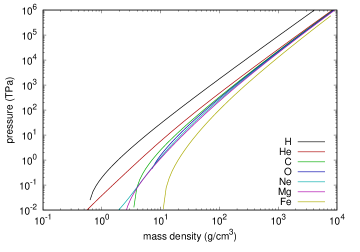
Figure 1: 1 K isotherm from AJ calculation.

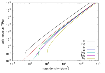
Figure 2: Bulk modulus from AJ calculation.

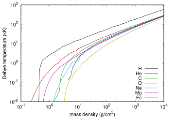
Figure 3: Debye temperature from AJ calculation (from Einstein temperature by equating energy).

The numerical solution of $G(B,\theta_{\text{D}})$ performed reliably over the full range of densities considered, for all elements (Fig. 4). The simplified calculation neglecting $B$ Ledbetter1991 gave results typically 30% higher.

The resulting $G(\rho)$ predictions were generated as tables. For convenience, we obtained functional fits to the tabular data: see Appendix.

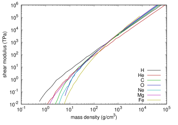
Figure 4: Summary of AJ shear modulus predictions at 1 K.

It is challenging to make EOS measurements at the terapascal range and above of materials that are solid at ambient conditions, and even more so to measure the shear modulus. For the elements considered here, our comparisons are primarily against ambient measurements where available, and otherwise against other models.

IV Previous shear modulus models

Other models have been developed for the shear modulus at high pressure. We summarize two of them here for which results have been published for Mg, C, and Fe.

IV.1 Steinberg-Guinan

The Steinberg-Guinan (SG) model Guinan1974 is widely used in hydrodynamic simulations below 100 GPa, and has the form

$$G=G_{0}\left[1+Ap/\eta^{1/3}-B(T-T_{0})\right]\quad:\quad\eta\equiv\rho/\rho_{0}$$ (4)

where $p$ is the pressure. Although developed for relatively low pressures, it is constructed to asymptote toward the one-component plasma (OCP) limit, where the shear modulus varies as $\rho^{4/3}$, if used in conjunction with an EOS model in which the pressure varies as $\rho^{5/3}$. However, the free parameters $G_{0}$, $A$, and $B$ are typically chosen to match low-pressure data, and the absolute value is not constrained to be correct in the OCP limit.

Improvements have been proposed to extend the SG model to higher pressures, either by adopting different parameter values in high-pressure phases Rudd2018 , or by modifying the dependence on compression to transition to a different function at high compressions Orlikowski2007 :

$$G = G_{0}\left\{f(\rho)G_{l}+\left[1-f(\rho)\right]G_{h}-B(T-T_{0})\right\}$$ (5)

$$f(\rho) = \left\{1+\exp\left[\alpha(\eta(\rho)-\eta_{c}\right]\right\}^{-1}$$ (6)

$$G_{l} = 1+A_{l}p/\eta(\rho)^{1/3}$$ (7)

$$G_{h} = A_{h}+M_{h}\eta(\rho)$$ (8)

$$\eta(\rho) = \rho/\rho_{0}.$$ (9)

Typically, the high pressure term $G_{h}$ is calibrated against electronic structure calculations that extend into the terapascal range, but do not explore the OCP limit. Ironically, it is the low pressure term $G_{l}$ that asymptotes to the expected OCP behavior, but is masked by the softer, linear dependence on $\rho$ in $G_{h}$.

As the SG and improved SG (ISG) models depend on the pressure as well as the mass density, an EOS is needed when calculating the shear modulus. For consistency across all models, we used the AJ EOS. The AJ method is typically less accurate at pressures below a few tenths of a terapascal, so other models may appear to be less accurate at low pressures than with alternative EOS.

IV.2 Straub

In theoretical studies using early electronic structure predictions, it was observed that the variation of shear modulus $G$ with the lattice parameter $a$ in cubic crystals such as W behaves similarly to the bulk modulus $B(a)$. A similar form of fitting function was adopted as was used for the cold curve energy $E(a)$,

$$G=G_{0}+g_{a}\frac{a-a_{0}}{a^{2}}e^{-g_{2}(a-a_{0})}.$$ (10)

Parameters were fitted to electronic structure datapoints $\{a_{i},G_{i}\}$ or to $G_{0}$ and $d\,\ln\,G/d\,\ln\,a$ Straub1990 . Shear moduli have been predicted in this way for a small number of elements, and included as tabulations of $G(\rho)$ in the sesame library of material properties sesame .

V Discussion

The AJ method is known to be inaccurate at low pressure in comparison with multi-ion electronic structure techniques, and the derived calculation of shear modulus involves unquantified approximations. In particular, the AJ method does not account for angular forces such as occur in molecular bonds. It is interesting to compare with a recent analysis invoking the shear contribution to the longitudinal sound speed $c_{l}$ in atomic matter, and comparing with high-fidelity electronic structure calculations of H Trachenko2020 . $c_{l}$ calculated from the AJ shear and bulk moduli agrees very well at low pressures with the theoretical analysis, to which multi-ion electronic structure calculations asymptote as H₂ molecules dissociate on compression. However, we find that $c_{l}$ is dominated by the contribution from $B$ for H in this regime, $G$ being $\sim 50$ times smaller than $B$.

For C, the AJ shear modulus falls well below the observed value for diamond at STP, which is not surprising for a structure stabilized by directional bonding. The prediction passes through our recent pseudopotential predictions Swift_dia_2020 above 10 g/cm³, crossing the Hill average just below 20 g/cm³ where the diamond structure was predicted to start to become unstable, and at higher is more consistent with an extrapolation of the Voigt polycrystal average in diamond. (Fig. 5).

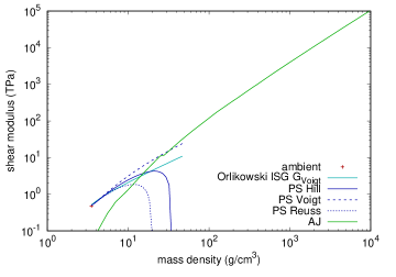
Figure 5: Comparison of AJ shear modulus prediction with observed and calculated behavior for C, including pseudopotential based multi-ion calculations (PS) Swift_dia_2020 and ISG model Orlikowski2007 . Pseudopotential predictions demonstrate possible range of shear modulus related to texture, and localized reductions in shear modulus associated with mechanical instability at a phase transition.

For Mg, which adopts the hexagonal close-packed structure at low pressures, the AJ shear modulus reproduces the observed STP value to within a few percent. It follows the SG model quite closely over a wide pressure range. The SG model appears to have a discrepancy at low pressures; as discussed above, this is an artifact caused by using the AJ EOS to calculate the pressure, and is an example of better performance of electronic structure calculations in predicting derivatives of pressure than for the pressure itself Akbarzadeh1993 . The AJ prediction becomes quite close to the SG model above 10 g/cm³ ($\sim$1 TPa), and as the compression increases further, the AJ shear modulus gradually becomes a few tens of percent stiffer than the SG. The SG model in this regime is constrained only by its asymptotic form, and this result is an example of the SG model performing remarkably well. Mg exhibits solid-solid phase transitions Pickard2010 ; Li2010 , but the observed and predicted structures are close-packed structures or perturbations of simple structures stabilized by interactions between inner electrons at high pressures, and the AJ calculation is likely to be reasonable for bulk average mechanical properties. (Fig. 6).

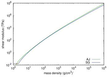
Figure 6: Comparison of AJ shear modulus prediction for Mg with STP measurement and SG model.

Fe exhibits solid phases, the low-pressure bcc structure being stabilized by magnetism, which the AJ model does not capture. The shear modulus of Fe at STP depends on the C content: low-C steels tend to be less rigid, and the AJ shear modulus lies relatively close to the lower reported values at STP. The Straub model is more consistent with C-rich Fe at low pressures, then passes through the AJ calculation around 4 TPa and lies well below at higher pressures. A SG calibration has been made for Fe at pressures of a few hundred gigapascals using multi-ion electronic structure calculations Rudd2009 . The AJ shear modulus intersects this model around 200 GPa and lies well below it at higher pressures. We suggest that these comparisons on balance favor the AJ calculation over a wide range of pressures. (Fig. 7).

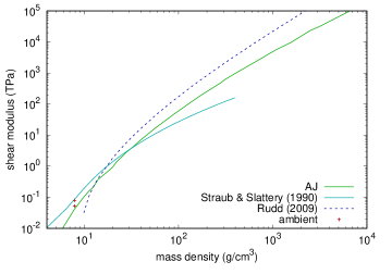
Figure 7: Comparison of AJ shear modulus prediction for Fe with STP measurements and models, including the Straub model which is sesame table 32140 ses32140 and the ISG model derived from multi-ion electronic structure calculations to the hundred gigapascal regime Rudd2009 .

Shear modulus predictions based on multi-ion electronic structure are more accurate in principle than the AJ predictions presented here. However, in practice, differences in technique and the need to calculate and combine multiple elastic moduli means that larger variations are commonly seen Swift_dia_2020 , and it has been difficult in practice to generate wide-range predictions of shear modulus. Also, multi-ion calculations must be performed in a mechanically-stable phase, involving extra effort to identify an appropriate phase at each state. Dynamic loading experiments have commonly been performed outside the range of meaningful estimates of the shear modulus: this is no longer necessary for elements Swift_ajsheardata_2020 . In high-pressure experiments, material strength is often a small effect in response dominated by the scalar EOS, and uncertainties $\sim 10\%$ in shear modulus appear correspondingly smaller in the overall response of the material. Because most materials are elastically anisotropic at some level, the effective shear modulus depends on the microstructural texture of the material, which may evolve during dynamic loading. Compared with microstructural effects (Fig. 5), an uncertainty $\sim 10\%$ is potentially insignificant.

VI Conclusions

Shear moduli were predicted for condensed matter from zero pressure to beyond the OCP regime using predictions of the bulk modulus and $\theta_{\text{D}}$ from AJ theory. Although the predicted shear moduli are likely to be inaccurate for crystal structures stabilized by angular forces, which are not captured by AJ theory, they appear to be a reasonable choice over a wide range of compressions when a more rigorous model is not available. The likely accuracy of the shear modulus predictions reflects the uncertainties in the underlying methods: the approach adopted here could be used with more accurate treatments of electronic structure when the corresponding calculations of elastic moduli are not available, for instance for alloys and compounds.

Electronic structure calculations using the AJ method are often inaccurate around zero pressure, but appear to be accurate above a few hundred gigapascals, depending on the element. The method is valid to extreme relativistic conditions – beyond the OCP regime – of density and temperature. AJ does not capture crystal structures and directional bonding: it is likely to be inaccurate in low-pressure structures or around phase transitions, maybe by $\sim$100%. As with other pressure derivatives, the shear modulus otherwise seems to be predicted more accurately than the absolute pressure. Aside from numerical noise in the nuclear perturbation calculation, the calculation of $\theta_{\text{D}}$ is an approximate average. The inaccuracy may be of order 10%, though predicted trends are likely to be better.

The likely performance correlates with the crystal structure. Non-close-packed structures at low pressure are represented poorly in the AJ electron model, so the ion model and EOS are likely to be inaccurate. AJ typically fails to predict bound matter at the observed zero-pressure density. The shear modulus is then also likely to be inaccurate, except for fortuitous cancellations of error. Close-packed structures are captured reasonably in the AJ electronic model, particularly at elevated pressure, so the ion model and EOS are likely to be reasonable, as is the shear modulus. As for the bulk modulus, the shear modulus seems to be predicted more accurately than the absolute pressure. The performance is probably similar for amorphous and glassy structures. For lower-symmetry structures at high pressure, when these are perturbations to, or stacking faults in, close-packed structures, the quality of shear modulus predictions is likely to be similar to that for the close-packed structures. Open structures stabilized by strong directional bonds are likely to be less accurate. In unstable and mixed phases, the shear modulus may be small, which is not captured in the AJ predictions. The performance should not however be affected by whether a structure is metastable or not.

We have also developed a functional form capable of representing the AJ shear moduli over a wide range, although it is not valid over the full range of the AJ calculations.

VII Appendix: Fit to AJ predictions

We tried using existing strength models to fit the AJ shear modulus data, but did not manage to find parameter sets valid over the wide range of density of the AJ calculations. This is not to claim that reasonable fits are impossible to find, but fitting involves iterative optimization of parameters with a non-linear dependence on the goodness of fit, which are often susceptible to numerical problems. A more general structure of model might involve a set of somewhat different functional forms valid over restricted ranges of density, with a transition function between each, as in the ISG model for diamond Orlikowski2007 . We were unable to determine significant parameter values for a separate power dependence from the AJ shear modulus predictions at low density. Instead, reasonable fits were obtained using a single value at the reference density and the switching function itself to describe stiffening at low compression:

$$G(\rho)=G_{0}f(\rho)+G_{1}\left(\frac{\rho}{\rho_{0}}\right)^{p_{1}}\left[1-f(\rho)\right]$$ (11)

where

$$f(\rho)=\exp\left(-\frac{\mu(\rho)}{\mu_{t}}\right)\quad:\quad\mu(\rho)\equiv\frac{\rho}{\rho_{0}}-1$$ (12)

and $G_{0}$, $G_{1}$, $p_{1}$ and $\mu_{t}$ are parameters. This functional form does not capture the AJ predictions in expansion, but this region is explored little in practice as materials spall in tension, limiting the distension of the bulk material. In general, this functional form does not represent the AJ shear modulus to the OCP regime with satisfactory accuracy at intermediate compressions, so the exponent $p_{1}$ was included as a parameter in a finite-range fit. (Table 1.)

Table 1: Fitting parameters for AJ shear modulus.

	$\rho_{0}$	$G_{0}$	$\mu_{t}$	$G_{1}$	$p_{1}$	Notes
	(g/cm3)	(GPa)		(GPa)
H	0.5	14.5	3.0	82	1.43	$\geq\rho_{0}$, which is arbitrary, and $\leq$500 g/cm3.
H	0.5	15	3.9	103	1.379	$\geq\rho_{0}$, which is arbitrary, and $\leq 5\times 10^{5}$ g/cm3.
He	0.5	0.3	26	55	1.390	$\geq$2 g/cm3. $\rho_{0}$ is arbitrary. $G_{0}$ is consistent with zero.
C	3.52	280	13	$1.64\times 10^{3}$	1.378	$\geq$7 g/cm3
O	6	24	11.6	$3.6\times 10^{3}$	1.392	$\geq\rho_{0}$, which is arbitrary.
Ne	4.8	900	22	$2.7\times 10^{3}$	1.40	$\geq$20 g/cm3. $\rho_{0}$ is arbitrary.
Ne	4.8	600	7.3	$1.0\times 10^{3}$	1.57	for 12 to 5000 g/cm3. $\rho_{0}$ is arbitrary.
Mg	1.738	$3.0\times 10^{4}$	140	$8.0\times 10^{2}$	1.39	$\geq$100 g/cm3
Mg	1.738	19	1.8	87	1.73	for 3 to 1000 g/cm3
Fe	7.874	52.5	9.3	$1.2\times 10^{3}$	1.68

Where possible, the STP values of $\rho$ and $G$ were used as parameters, and low pressure AJ points were deweighted or removed if necessary. Otherwise, such as where AJ fails to capture solid phases with a significantly different shear modulus, the AJ data were fitted as far down in pressure as possible, $G_{0}$ was fitted if necessary, and $\rho_{0}$ was also adjusted if needed to keep $G_{0}>0$. The resulting models are not intended for use at low pressure, though some are probably adequate for practical purposes.

The fitted equation usually matches the AJ data to within a few percent. Between numerical noise in the AJ calculation and probably-physical structure not captured by the equation, the deviation could be up to 20% in some places in most models, and 30% in a few (Figs 8 to 17).

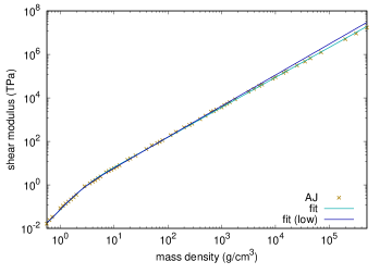
Figure 8: Comparison of AJ shear modulus predictions for H with fits.

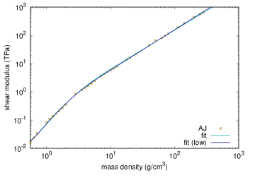
Figure 9: Comparison of AJ shear modulus predictions for H with fits (detail at lower compression).

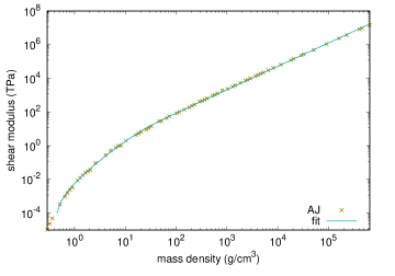
Figure 10: Comparison of AJ shear modulus predictions for He with fit.

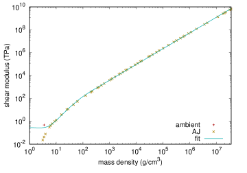
Figure 11: Comparison of AJ shear modulus predictions for C with fit.

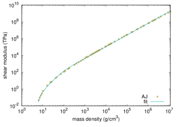
Figure 12: Comparison of AJ shear modulus predictions for O with fit.

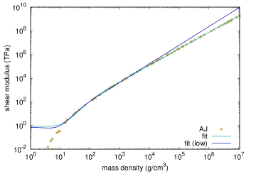
Figure 13: Comparison of AJ shear modulus predictions for Ne with fit.

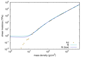
Figure 14: Comparison of AJ shear modulus predictions for Ne with fits (detail at lower compression).

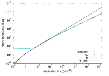
Figure 15: Comparison of AJ shear modulus predictions for Mg with fits.

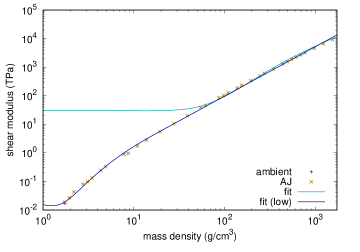
Figure 16: Comparison of AJ shear modulus predictions for Mg with fits (detail at lower compression).

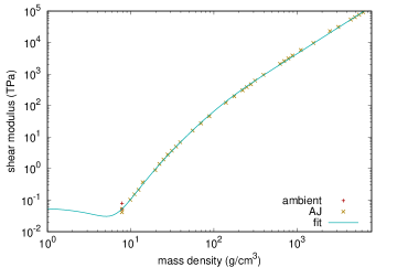
Figure 17: Comparison of AJ shear modulus predictions for Fe with fit.

References

- (1) For instance, R.E. Rudd, L.H. Yang, P.D. Powell, P. Graham, A. Arsenlis, R.M. Cavallo, A.G. Krygier, J.M. McNaney, S.T. Prisbrey, B.A. Remington, D.C. Swift, C.E. Wehrenberg, and H.-S. Park, Am. Inst. Phys. Conf. Proc. 1979, 070027 (2018).
- (2) D.C. Swift, O. Heuzé, A. Lazicki, S. Hamel, L.X. Benedict, R.F. Smith, J.M. McNaney, and G.J. Ackland, arXiv:2004.03071 (2020).
- (3) D.A. Liberman, Phys. Rev. B 20, 12, 4981 (1979).
- (4) D.A. Liberman and B.I. Bennett, Phys. Rev. B 42, 2475 (1990).
- (5) D.C. Swift, T. Lockard, M. Bethkenhagen, R.G. Kraus, L.X. Benedict, P. Sterne, M. Bethkenhagen, S. Hamel, and B.I. Bennett, Phys. Rev. E 99, 063210 (2019).
- (6) D.C. Swift, T. Lockard, M. Bethkenhagen, S. Hamel, A. Correa, L.X. Benedict, P.A. Sterne, and B.I. Bennett, Phys. Rev. E 101, 053201 (2020).
- (7) D.C. Swift, T. Lockard, S. Hamel, C.J. Wu, L.X. Benedict, P.A. Sterne, and H.D. Whitley, arXiv:2103.03371 (2021).
- (8) D.C. Swift, G.J. Ackland, A. Hauer, and G.A. Kyrala, Phys. Rev. B 63, 214107 (2001).
- (9) E. Madelung, Phys. Z. 11, 898 (1910).
- (10) A. Einstein, Ann. Phys. Leipzig 34, 170 (1911).
- (11) O.L. Anderson, J. Phys. Chem. Solids 24, 909 (1963).
- (12) For instance, X Liu and H.-Q. Fan, R. Soc. open sci. 5, 171921 (2018).
- (13) H. Ledbetter, Z. Metallkd. 82, 820 (1991).
- (14) E. Kröner, Z. Phys. 151, 504 (1958).
- (15) M.W. Guinan and D. Steinberg, J. Phys. Chem. Solids 35, 1501 (1974).
- (16) D. Orlikowski, A.A. Correa, E. Schwegler, and J.E. Klepeis, Am. Inst. Phys. Conf. Proc. 955, pp. 247–250 (2007).
- (17) G. Straub, Los Alamos National Laboratory report LA-11806-MS (1990).
- (18) S.P. Lyon and J.D. Johnson, Los Alamos National Laboratory report LA-UR-92-3407 (1992).
- (19) D.A. Young and E.M. Corey, J. Appl. Phys. 78, 3748 (1995).
- (20) K. Trachenko, B. Monserrat, C.J. Pickard, and V.V. Brazhkin, Science Adv. 6, 41, eabc8662 (2020).
- (21) H. Akbarzadeh, S.J. Clark, and G.J. Ackland, J. Phys: Cond. Matt. 5, 8065 (1993).
- (22) C.J. Pickard and R.J. Needs, Nature Materials 9, 624 (2010).
- (23) P. Li, G. Gao, Y. Wang, and Y. Ma, J. Phys. Chem. C 114, 21745 (2010).
- (24) R. Rudd (Lawrence Livermore National Laboratory), private communication.
- (25) G. Straub and W. Slattery (Los Alamos National Laboratory), documentation for sesame model 32140 (1990).
- (26) D.C. Swift, Lawrence Livermore National Laboratory report LLNL-TR-814454 (2020); https://gdo-hdp.llnl.gov/matprops/aj/shearfit.html