A Variational Surface-Evolution Perspective for Optimal Transport between Densities with Differing Compact Support

Abstract

We examine the optimal mass transport problem in $\mathbb{R}^{n}$ between densities having independent compact support by considering the geometry of a continuous interpolating support boundary in space-time within which the mass density evolves according to the fluid dynamical framework of Benamou and Brenier. We treat the geometry of this space–time embedding in terms of points, vectors, and sets in $\mathbb{R}^{n+1}\!=\mathbb{R}\times\mathbb{R}^{n}$ and blend the mass density and velocity as well into a space-time solenoidal vector field ${\bf W}\;|\;{\bf\Omega\subset}\mathbb{R}^{n+1}\!\to\mathbb{R}^{n+1}$ over compact sets ${\bf\Omega}$ . We then formulate a coupled gradient descent approach containing separate evolution steps for $\partial{\bf\Omega}$ and ${\bf W}$.

1 Introduction

Optimal mass transport (OMT) has a long history, beginning with Gaspard Monge [1] in 1781, and put into a more modern form solvable via linear programming by Leonid Kantorovich [2, 3, 4, 5, 6, 7]. In recent years, OMT has undergone a huge surge, with many diverse applications including signal/image processing, computer vision, machine learning, data analysis, meteorology, statistical physics, quantum mechanics, and network theory [8, 9, 10, 11, 12, 13].

Our interest in the present work is extending the Benamou and Brenier computational fluid dynamical (CFD) to OMT where the domains have compact support. We recall that in the seminal work [14], Benamou and Brenier compute the Wasserstein 2-metric $W_{2}$ via the minimization of kinetic energy subject to a continuity constraint. They moreover compute the optimal path (i.e., geodesic) in the space of probability densities [15]. In image processing, this gives a natural interpolation path between two images, where the intensity is treated as a “generalized mass.” This is important for problems in deformable registration and image warping; see [16, 17] and the references therein..

Now the method of Benamou and Brenier does not take into account that the regions of interest in images are in fact compact, and so the computations cannot be performed on a regular grid and crucially boundary conditions must be imposed. It is this issue that motivated the present work. To treat the problem of OMT on densities with compact support, we propose a synergy of methods from OMT as well as level set evolutions [18, 19]. Level set methods are a powerful way of implementing interface (boundary) evolution problems and thus have become a standard for a number of approaches in computer vision for segmentation, so-called active contour methods; see [20] and the references therein.

This synergy of level sets and OMT, we believe to be novel, and to potentially have a number of applications, in particular to digital pathology.

2 Spatiotemporal hypersurface

We use bold notation exclusively to denote space-time points, vectors, and sets and non-bold notation for similar entities in time or space only, as well as for scalar variables. Accordingly, ${\bf X}$ will represent an arbitrary spatiotemporal point in $\mathbb{R}^{n+1}$

$${\bf X}=(t,x)=(\underbrace{X_{0}}_{t},\underbrace{X_{1},X_{2},\ldots,X_{n}}_{x})$$

which pairs a temporal coordinate $t\in\mathbb{R}$ with a spatial coordinate $x\in\mathbb{R}^{n}$. We will denote the spatiotemporal basis vectors by ${\bf e_{0}},{\bf e}_{1},{\bf e}_{2},\ldots,{\bf e}_{n}$ so that

$${\bf X}=\underbrace{X_{0}\,{\bf e}_{0}}_{t}+\underbrace{X_{1}\,{\bf e}_{1}+X_{2}\,{\bf e}_{2}+\cdots+X_{n}\,{\bf e}_{n}}_{x}$$

2.1 Assumptions

Compact support

We consider a spatiotemporal density $\rho$ in the form of a positive scalar function ${\bf X}\to\rho({\bf X})$ in $\mathbb{R}^{n+1}$ whose restriction to the $t\!=\!0$ hyperplane matches a given initial spatial density $\rho_{0}$ and whose restriction to the $t\!=\!1$ hyperplane matches a given spatial target density $\rho_{1}$. We assume the initial spatial density $\rho_{0}$ has compact support $\Omega_{0}\subset\mathbb{R}^{n}$ and that the target spatial density $\rho_{1}$ has compact support $\Omega_{1}\subset\mathbb{R}^{n}$. We further assume that the full spatiotemporal density $\rho$ also has compact support ${\bf\Omega}\subset\mathbb{R}^{n+1}$ in space-time, sandwiched between the hyperplanes $t\!=\!0$ and $t\!=\!1$, which may be constructed by a continuous family of intermediate compact spatial supports $\Omega_{[t]}\subset\mathbb{R}^{n}$ with $\Omega_{[0]}=\Omega_{0}$ and $\Omega_{[1]}=\Omega_{1}$ as follows.

$${\bf\Omega}=\left\{{\bf X}=(t,x)\;|\;0\leq t\leq 1\,,\,x\in\Omega_{[t]}\right\}$$ (1)

Balanced density

We assume the initial and target spatial densities $\rho_{0}$ and $\rho_{1}$ both have unit mass. We impose a similar constraint on the spatiotemporal density $\rho$, summarizing these assumptions as follows.

$$\int_{\Omega_{0}}\rho_{0}(x)\,dx=\int_{\Omega_{1}}\rho_{1}(x)\,dx=\int_{{\bf\Omega}}\rho({\bf X})\,d{\bf X}=1$$ (2)

Smoothness

We assume the initial and target spatial densities $\rho_{0}$ and $\rho_{1}$ are differentiable within their support $\Omega_{0}$ and $\Omega_{1}$ and that the spatiotemporal density $\rho$ is differentiable within its support ${\bf\Omega}$. We also assume that the portion of the spatiotemporal boundary $\partial{\bf\Omega}$ that lies strictly within $0\!<\!t\!<\!1$, which we denote by ${\bf\Gamma}$, is differentiable. The remaining portions of $\partial{\bf\Omega}$ are provided by the embeddings of $\Omega{}_{0}$ and $\Omega_{1}$ within the hyperplanes $t\!=\!0$ and $t\!=\!1$ to form two flat temporal faces of ${\bf\Omega}$, which we denote by ${\bf\Gamma}_{0}$ and ${\bf\Gamma}_{1}$.

Piece-wise smooth boundary

As such $\partial{\bf\Omega={\bf\Gamma}}\cup{\bf\Gamma}_{0}\cup{\bf\Gamma}_{1}$ will have the form of a compact hypersurface in $\mathbb{R}^{n+1}$ with a well defined outward normal everywhere except along the borders of the two temporal faces where ${\bf\Gamma}_{0}$ and ${\bf\Gamma}_{1}$ connect to the intervening surface ${\bf\Gamma}$. We may also describe the intervening spatiotemporal boundary component ${\bf\Gamma}$ as the swept out surface generated by embedding the boundaries $\Gamma_{[t]}=\partial\Omega_{[t]}$ of the deforming spatial supports $\Omega_{[t]}$ into the corresponding temporal hyperplanes. The spatiotemporal boundary notation and decomposition is summarized as follows.

$$\partial{\bf{\bf\Omega}}=\underbrace{\left\{{\bf X}=(0,x)\;|\;x\in\Omega_{0}\right\}}_{\underset{\mbox{(temporal face)}}{{\bf\Gamma}_{0}}}\cup\underbrace{\left\{{\bf X}=(1,x)\;|\;x\in\Omega_{1}\right\}}_{\underset{\mbox{(temporal face)}}{{\bf\Gamma}_{1}}}\cup\underbrace{\left\{{\bf X}=(t,x)\;|\;0\leq t\leq 1\,,\,x\in\overbrace{\partial\Omega_{[t]}}^{\Gamma_{[t]}}\right\}}_{\underset{\mbox{(swept out surface)}}{{\bf\Gamma}}}$$ (3)

2.2 Local geometry

In this section we explore the relationship between the local geometry of the spatial support boundary $\Gamma_{[t]}$ and the swept out spatiotemporal boundary ${\bf\Gamma}$.

Parameterization

Let $s=(s_{1},\ldots,s_{n-1})$ represent isothermal coordinates with unit speed at a point $x\in$$\Gamma_{[t]}$ along the boundary of the spatial support $\Omega_{[t]}\subset\mathbb{R}^{n}$ at time $t$ strictly between 0 and 1, The Riemannian metric tensor of $\Gamma_{[t]}$ in these coordinates is therefore the $(n-1)\times(n-1)$ identity matrix at the point $x$ with $n-1$ orthonormal tangent vectors $\frac{\partial\Gamma_{[t]}}{\partial s_{k}}\in\mathbb{R}^{n}$ for $k=1,\ldots,n-1$. From (3) we know that the corresponding spatiotemporal point ${\bf X}=(t,x)$ belongs to portion ${\bf\Gamma}$ of the spatiotemporal support boundary $\partial{\bf\Omega}$, which may be locally parameterized as follows.

$${\bf\Gamma}(t,s)=\left(t,\Gamma_{[t]}(s)\right)=(\underbrace{\Gamma_{0}}_{t},\underbrace{\Gamma_{1},\Gamma_{2},\ldots,\Gamma_{n}}_{\Gamma_{[t]}(s)})$$ (4)

Unit normal

In these coordinates, we compute the following $n$ tangent vectors to ${\bf\Gamma}$ in $\mathbb{R}^{n+1}$

$$\frac{\partial{\bf\Gamma}}{\partial t}=\left(1,\frac{\partial\Gamma_{[t]}}{\partial t}\right)\quad\mbox{and}\quad\frac{\partial{\bf\Gamma}}{\partial s_{k}}=\left(0,\frac{\partial\Gamma_{[t]}}{\partial s_{k}}\right),\text{$\quad k=1,\ldots,n-1$}$$ (5)

Since the unit outward normal $N\in\mathbb{R}^{n}$ to the spatial boundary $\Gamma_{[t]}$ is orthogonal to the $n-1$ spatial tangent vectors $\frac{\partial\Gamma_{[t]}}{\partial s_{k}}\in\mathbb{R}^{n}$, it is clear to see that $(\alpha,N)\in\mathbb{R}^{n+1}$ will be orthogonal to the $n-1$ spatiotemporal tangent vectors $\frac{\partial{\bf\Gamma}}{\partial s_{k}}$ expressed in (5) for any choice of scalar $\alpha$. Orthogonality to the additional spatiotemporal tangent vector $\frac{\partial{\bf\Gamma}}{\partial t}$ expressed in (5) as well requires $\alpha=-\frac{\partial\Gamma_{[t]}}{\partial t}\cdot N$, yielding the following construction of the spatiotemporal unit outward normal ${\bf N}\in\mathbb{R}^{n+1}$.

$$\text{{\bf N}}=\begin{cases}\frac{\left(-\frac{\partial\Gamma_{[t]}}{\partial t}\cdot N,N\right)}{\sqrt{1+\left(\frac{\partial\Gamma_{[t]}}{\partial t}\cdot N\right)^{2}}},&\text{{\bf X}}\in{\bf\Gamma}\\ +{\bf e}_{0}=+(1,0,\ldots,0),&\text{{\bf X}}\in{\bf\Gamma}_{1}\\ -{\bf e}_{0}=-(1,0,\ldots,0),,&\text{{\bf X}}\in{\bf\Gamma}_{0}\end{cases}$$ (6)

Metric tensor

Using the tangent vectors (5) we may express the Riemannian metric tensor at the point ${\bf X}$ in the form of the following $n\times n$ matrix

$$\underbrace{{\bf I}(s_{1},\ldots,s_{n-1},t)}_{\mbox{I-fundamental form}}=\begin{bmatrix}{\cal I}&\left(\frac{\partial\Gamma_{[t]}}{\partial s}\right)^{T}\frac{\partial\Gamma_{[t]}}{\partial t}\\ \frac{\partial\Gamma_{[t]}}{\partial t}^{T}\left(\frac{\partial\Gamma_{[t]}}{\partial s}\right)&1+\frac{\partial\Gamma_{[t]}}{\partial t}\cdot\frac{\partial\Gamma_{[t]}}{\partial t}\end{bmatrix}$$ (7)

where $\frac{\partial\Gamma_{[t]}}{\partial s}$ denotes the $n\times(n-1)$ matrix whose columns consist of the orthonormal tangent vectors to the spatial boundary $\Gamma_{[t]}$ at the point $x$. Using the determinant formula, $\det\begin{bmatrix}A&u\\ v^{T}&\alpha\end{bmatrix}=\alpha\det A-v^{T}\mbox{adj}A\,u$ (for any matrix $A$, vector $u$ and $v$, and scalar $\alpha$), we may compute.

$$\det{\bf I}=\left(1+\frac{\partial\Gamma_{[t]}}{\partial t}\cdot\frac{\partial\Gamma_{[t]}}{\partial t}\right)-\underbrace{\sum_{k=1}^{n-1}\left(\frac{\partial\Gamma_{[t]}}{\partial s_{k}}\cdot\frac{\partial\Gamma_{[t]}}{\partial t}\right)^{2}}_{\left\|\frac{\partial\Gamma_{[t]}}{\partial t}\right\|^{2}-\left(\frac{\partial\Gamma_{[t]}}{\partial t}\cdot N\right)^{2}}=1+\left(\frac{\partial\Gamma_{[t]}}{\partial t}\cdot N\right)^{2}$$

Area element

The relationship between the area element $dS_{[t]}$ of the spatial boundary surface $\Gamma_{[t]}$, the temporal element $dt$, and the area element $d{\bf S}$ of the swept out spatiotemporal hypersurface ${\bf\Gamma}$ can be expressed via the square root of the determinant of the first fundamental form shown above.

$$d{\bf S}=\sqrt{1+\left(\frac{\partial\Gamma_{[t]}}{\partial t}\cdot N\right)^{2}}dS_{[t]}\,dt$$ (8)

Normal variations

Finally, using the parameterization (4) for a variation $\delta{\bf{\bf\Gamma}}$ allows us to relate a variation of the swept out spatiotemporal hypersurface to time parameterized variations $\delta\Gamma_{[t]}$ of the spatial support boundaries as follows $\delta{\bf{\bf\Gamma}}=\left(0,\delta\Gamma_{[t]}\right)$. Combining this with (6) yields the following relationship between variations of $\Gamma_{[t]}$ and variations of ${\bf\Gamma}$ along their respective normal directions.

$$\delta{\bf{\bf\Gamma}}\cdot{\bf N}=\frac{\delta\Gamma_{[t]}\cdot N}{\sqrt{1+\left(\frac{\partial\Gamma_{[t]}}{\partial t}\cdot N\right)^{2}}}$$

If we now further combine this with (8) we see that the normal variation of the spatiotemporal hypersurface measured against its spatiotemporal area element matches the normal variation of the corresponding spatial boundary measured by its respective area element and time element.

$$\left(\delta{\bf{\bf\Gamma}}\cdot{\bf N}\right)\,d{\bf S}=\left(\delta\Gamma_{[t]}\cdot N\right)\,dS_{[t]}\,dt$$ (9)

3 Spatiotemporal formulation of optimal mass transport

The fluid dynamical framework of Benamou and Brenier, considers two time evolving entities, a scalar mass density $\rho(t,x)$ and a velocity field $v(t,x)\in\mathbb{R}^{n}$ which are coupled by the local mass preserving continuity constraint $\frac{\partial\rho}{\partial t}+\nabla_{x}\cdot(\rho v)=0$.

Notice that in the standard manner regarding $\rho v$ as an ordinary 3-vector, the continuity constraint means that density and spatial momentum form a 4-vector with respect to the standard Minkowski metric in the standard physics setting [21]. We will exploit this observation and develop an equivalent formulation using a single space-time solenoidal vector field ${\bf W}$ with simple normal boundary conditions along the spatiotemporal hypersurface $\partial{\bf\Omega}$ that enable convenient numerical solutions of PDE’s directly within on an $n+1$ dimensional space-time grid, with no need to treat the temporal and spatial dimensions separately or differently.

3.1 Spatiotemporal advection field ${\bf U}$

We begin by noting that in the combined spatiotemporal variable ${\bf X}=(t,x)$, the continuity constraint $\frac{\partial\rho}{\partial t}+\nabla_{x}\cdot(\rho v)=0$ can be written as

$$\nabla\rho\cdot{\bf U}+\rho\nabla\cdot{\bf U}=0$$ (10)

where $\nabla$ and $\nabla\cdot$ represent the full spatiotemporal gradient and divergence operators in $\mathbb{R}^{n+1}$ and where ${\bf U}\in\mathbb{R}^{n+1}$ denotes the following vector field.

$${\bf U}({\bf X})\dot{=}\left(1,v\right)=(\underbrace{U_{0}}_{1},\underbrace{U_{1},U_{2},\ldots,U_{n}}_{v})$$

Note that ${\bf U}$ is tangent to the characteristics of this linear first order PDE (10) in $\rho$ and therefore defines the trajectories along which mass is transported across space-time. Since the spatiotemporal hypersurface $\partial{\bf\Omega}$, more specifically its swept out portion ${\bf\Gamma}$, defines the boundary of the evolving support for $\rho$, we can conclude that these advection trajectories must flow along the hypersurface ${\bf\Gamma}$ itself, never across it (neither inward nor outward). In other words, mass cannot be transported outside of its support neither forward in time (which excludes outward-flowing characteristics) nor backward in time (which excludes inward-flowing characteristics). This leads to the boundary condition ${\bf U}\cdot{\bf N}=0$ along ${\bf\Gamma}$, which may be written in terms of $v$, $N$, and $\frac{\partial\Gamma_{[t]}}{\partial t}$ as follows.

$$\underbrace{v\cdot N=\frac{\partial\Gamma_{[t]}}{\partial t}\cdot N}_{({\bf U}\cdot{\bf N}=0)}$$ (11)

If we plug this constraint between the support evolution $\frac{\partial\Gamma_{[t]}}{\partial t}$ and the velocity field $v$ into (6) we obtain the following alternative expression for the outward unit normal ${\bf N}\in\mathbb{R}^{n+1}$ of the swept out hypersurface ${\bf\Gamma}$ in terms of the outward normal $N\in\mathbb{R}^{n}$ of the support boundary $\Gamma_{[t]}$ in space at time $t$.

$${\bf N}({\bf X}) =\frac{\left(-v\cdot N,N\right)}{\sqrt{1+\left(v\cdot N\right)^{2}}},\quad{\bf X}\in{\bf\Gamma}$$ (12)

3.2 Solenoidal vector field ${\bf W}$

While the use of the advection field ${\bf U}$ merges the spatial and temporal derivatives into a single derivative $\mathbb{R}^{n+1}$ operator in (11), it still keeps the density variable $\rho$ separate. We now merge these two entities by defining another spatiotemporal vector field whose first (temporal) component represents the mass density $\rho({\bf X})$, and whose remaining components represent the momentum vector ${\rm p}({\bf X})=\rho v$ in $\mathbb{R}^{n}.$

$${\bf W}({\bf X})=\rho{\bf U}=\left(\,\rho\,,\,{\rm p}\,\right)=(\underbrace{W_{0}}_{\rho},\underbrace{W_{1},W_{2},\ldots,W_{n}}_{\mbox{momentum }{\rm p}=\rho v})$$ (13)

However, rather than considering (13) to be the definition of ${\bf W}$ in terms of the density $\rho$ and momentum ${\rm p}$, we instead consider it in reverse to be the definition of $\rho$ and ${\rm p}$ in terms of the space-time vector field ${\bf W}$ subject to the continuity constraint (10) which now simplifies to a coordinate-free solenoidal condition on ${\bf W}$.

$$\nabla\cdot{\bf W}=0$$ (14)

Multiplying the boundary condition ${\bf U}\cdot{\bf N}=0$ along ${\bf\Gamma}$ presented in (11) by $\rho$ yields a similar vanishing flux condition for ${\bf W}$ across the swept out portion of the spatiotemporal hypersurface $\partial{\bf\Omega}$. For the remainder of $\partial{\bf\Omega}$, we combine ${\bf N}=\text{$\pm$}{\bf e}_{0}$ from (6) with (13) to obtain flux conditions for ${\bf W}$ along the temporal faces ${\bf\Gamma}_{0}$ and ${\bf\Gamma}_{1}$ as well, in terms of the known starting and target densities $\rho_{0}$ and $\rho_{1}$.

The combination of these constraints is easily summarized now in terms of ${\bf W}$ and its spatiotemporal domain ${\bf\Omega}$. Namely we seek a solenoidal vector field ${\bf W}$ within ${\bf\Omega}$ with the following prescribed flux conditions along the full spatiotemporal domain boundary $\partial{\bf{\bf\Omega}}$.

$${\bf W}\cdot{\bf N}=\begin{cases}\;\;0\;\;,&{\bf X}\in{\bf\Gamma}\\ -\rho_{0},&{\bf X}\in{\bf\Gamma}_{0}\\ +\rho_{1},&{\bf X}\in{\bf\Gamma}_{1}\end{cases}$$ (15)

3.3 Extended velocity ${\bf V}$

Local kinetic energy

Before setting up the variational problem we seek an expression for the local measure of kinetic energy ${\rm T}(t,x)$

$${\rm T}({\bf X})=\frac{1}{2}\rho\,v\cdot v$$

in terms of the solenoidal field ${\bf W}$. If we express this purely in terms of ${\bf W}$, we obtain the following expression which, unfortunately, is not coordinate free.

$${\rm T}({\bf X})=\frac{1}{2}\left(\frac{\overbrace{{\bf W}\cdot{\bf W}}^{\rho^{2}(1+v\cdot v)}}{\underbrace{{\bf W}\cdot{\bf e}_{0}}_{\rho}}-\underbrace{{\bf W}\cdot{\bf e}_{0}}_{\rho}\right)$$

Extended velocity

We may resolve this by introducing the following extended velocity field ${\bf V}\in\mathbb{R}^{n+1}$ which extends the transport velocity $v$ from $\mathbb{R}^{n}$ into $\mathbb{R}^{n+1}$ by adding a temporal component equal to $-\frac{1}{2}\|v\|^{2}$ as follows

$${\bf V}\doteq\left(-\frac{1}{2}\|v\|^{2}\,,\,v\right)=(\underbrace{V_{0}}_{\frac{-\|v\|^{2}}{2}},\underbrace{V_{1},V_{2},\ldots,V_{n}}_{v})$$ (16)

Notice that, just like the advection field ${\bf U}$, the extended velocity ${\bf V}$ depends only upon the spatial velocity $v$ itself, and therefore contains no additional information. We may now express the local kinetic energy compactly and coordinate free in terms of the solenoidal field ${\bf W}$ and the extended velocity field ${\bf V}$ by their inner product.

$${\rm T}={\bf W}\cdot{\bf V}$$

We summarize our notation for the three spatial-temporal vector fields in $\mathbb{R}^{n+1}$ as follows.

$$\begin{array}[]{ccc}\mbox{advection field}&\mbox{solenoidal field}&\mbox{extended velocity}\\ {\bf U}=(1,v)&{\bf W}=\rho{\bf U}=(\rho,{\rm p})&{\bf V}=\left(-\frac{1}{2}\|v\|^{2}\,,\,v\right)\end{array}$$

3.4 Variational formulation

3.4.1 Action integral

We begin by constructing the action integral to be minimized over ${\bf\Omega}\subset\mathbb{R}^{n+1}$ in terms of the solenoidal field ${\bf W}$ as follows.

$$\int_{0}^{1}\int_{\Omega_{[t]}}\overbrace{\frac{1}{2}\rho\|v\|^{2}}^{T}\,dx\,dt=\int_{{\bf\Omega}}{\bf W}\cdot{\bf V}\,d{\bf X}$$

Note that the two unknowns are only ${\bf W}$ and its support ${\bf\Omega}$ (or equivalently the swept out boundary ${\bf\Gamma}$) even though we have expressed the action compactly also in terms of ${\bf V}$. We may compute ${\bf V}$ directly from ${\bf W}$

$${\bf V}\,\doteq\left(-\frac{1}{2}\|v\|^{2}\,,\,v\right)={\bf U}-\frac{1}{2}\left({\bf U}\cdot{\bf U}+1\right){\bf e}_{0}=\frac{{\bf W}}{{\bf W}\cdot{\bf e}_{0}}-\frac{1}{2}\left(\frac{{\bf W}\cdot{\bf W}}{\left({\bf W}\cdot{\bf e}_{0}\right)^{2}}+1\right){\bf e}_{0}$$ (17)

with the following compatible flux conditions obtained by plugging in (15).

$${\bf V}\cdot{\bf N} =\begin{cases}-\left(1+\frac{1}{2}\|v\|^{2}\right)\left({\bf N}\cdot{\bf e}_{0}\right),&{\bf X}\in{\bf\Gamma}\\ +\frac{1}{2}\|v\|^{2},&{\bf X}\in{\bf\Gamma}_{0}\\ -\frac{1}{2}\|v\|^{2},&{\bf X}\in{\bf\Gamma}_{1}\end{cases}$$

Incorporating the solenoidal (mass preservation) constraint (14) through a Lagrange multiplier $\lambda$ over ${\bf{\bf\Omega}}$ and the flux constraints through an additional Lagrange multiplier $\alpha$ along the boundaries $\partial{\bf\Omega}={\bf\Gamma}_{0}\cup{\bf\Gamma}_{1}\cup{\bf\Gamma}$.

$$E=\int_{{\bf\Omega}}{\bf W}\cdot{\bf V}\,+\underbrace{\lambda\,\nabla\cdot{\bf W}}_{\stackrel{{\scriptstyle\mbox{solenoidal}}}{{\mbox{constraint}}}}\,d{\bf X}+\underbrace{\int_{{\bf\Gamma}}\alpha{\bf W}\cdot{\bf N}\,dS+\int_{{\bf\Gamma}_{0}}\alpha\left(\overbrace{{\bf W}\cdot{\bf N}}^{-{\bf W}\cdot{\bf{\bf e}_{0}}}+\rho_{0}\right)\,dS+\int_{{\bf\Gamma}_{1}}\alpha\left(\overbrace{{\bf W}\cdot{\bf N}}^{{\bf W}\cdot{\bf e}_{0}}-\rho_{1}\right)\,dS}_{\mbox{flux constraints}}$$ (18)

3.4.2 First variation

Next, we compute the variation of (18) to obtain (see Appendix 5.1)

$$\delta E= \int_{{\bf\Omega}}\delta{\bf W}\cdot\left({\bf V}-\nabla\lambda\right)\;d{\bf X}+\int_{{\bf\Gamma}}{\bf W}\cdot\left({\bf V}+\nabla_{S}\alpha\right)\delta{\bf\Gamma}\cdot{\bf N}\,dS$$ (19)

$$+\underbrace{\int_{{\bf\Gamma}}\left(\alpha+\lambda\right)\,\delta{\bf W}\cdot{\bf N}\,dS-\int_{{\bf\Gamma}_{0}}\left(\alpha+\lambda\right)\,\delta{\bf W}\cdot{\bf e}_{0}\,dS+\int_{{\bf\Gamma}_{1}}\left(\alpha+\lambda\right)\,\delta{\bf W}\cdot{\bf e}_{0}\,dS}_{\int_{\partial{\bf\Omega}}\left(\alpha+\lambda\right)\,\delta{\bf W}\cdot{\bf N}\,dS}$$

Necessary optimality condition

Optimality for ${\bf W}$ can only be achieved if we can solve

$$\nabla\lambda={\bf V}$$ (20)

for $\lambda$ within the interior of ${\bf\Omega}$ (additional conditions are required along the boundary to annihilate the boundary integrals as well). If we separately equate the spatial and temporal components

$$\overbrace{\Bigl{(}\underbrace{\frac{\partial\lambda}{\partial X_{0}}}_{\frac{\partial\lambda}{\partial t}},\underbrace{\frac{\partial\lambda}{\partial X_{1}},\frac{\partial\lambda}{\partial X_{2}},\ldots,\frac{\partial\lambda}{\partial X_{n}}}_{\frac{\partial\lambda}{\partial x}}\Bigr{)}}^{\nabla\lambda}=\overbrace{\Bigl{(}\underbrace{V_{0}}_{\frac{-\|v\|^{2}}{2}},\underbrace{V_{1},V_{2},\ldots,V_{n}}_{v}\Bigr{)}}^{{\bf V}}$$

then we see that (20) amounts to a more compact, coordinate-free expression of the well known Hamilton Jacobi equation.

$$\frac{\partial\lambda}{\partial t}+\frac{1}{2}\left\|\frac{\partial\lambda}{\partial x}\right\|^{2}=0$$ (21)

However, (20) will not admit a solution unless ${\bf V}$ is a conservative (irrotational) vector field. As such, the gradient must be related to the non-conservative (solenoidal) portion of the extended velocity field ${\bf V}$.

Helmoltz decomposition

Accordingly, we consider the Helmholtz decomposition to express ${\bf V}$ as the sum of two vector fields

$$\text{{\bf V}}=\underbrace{\text{{\bf V}}^{\parallel}}_{\stackrel{{\scriptstyle\mbox{irrotational}}}{{(\mbox{curl-free)}}}}+\underbrace{{\bf V}^{\perp}}_{\stackrel{{\scriptstyle\mbox{solenoidal}}}{{(\mbox{divergence-free})}}}$$ (22)

where ${\bf V}^{\perp}$ denotes the divergence free component ($\nabla\cdot{\bf V}^{\perp}=0$) and where ${\bf V}^{\parallel}$ denotes the curl free component ($\nabla\times{\bf V}^{\parallel}=0$) which can be written as the gradient of a scalar potential function ${\bf V}^{\|}=\nabla\phi$. However, this decomposition is not unique over compact domains. We obtain the decomposition by solving the following Poisson equation for a scalar potential function $\phi$.

$$\Delta\phi =\nabla\cdot{\bf V},\quad{\bf X}\in{\bf\Omega}$$ (23)

and can therefore parameterize the set of all possible decompositions by the choice of imposed boundary conditions along $\partial{\bf\Omega}$. To maintain the initial and final density constraints, Neumann boundary conditions must be imposed on the two temporal faces ${\bf\Gamma}_{0}$ and ${\bf\Gamma}_{1}$

$$\nabla\phi\cdot{\bf N} =\overbrace{{\bf V}\cdot{\bf N}}^{-{\bf V}\cdot{\bf e}_{0}}=+\frac{1}{2}\|v\|^{2},\;{\bf X}\in{\bf\Gamma}_{0}$$ (24)

$$\nabla\phi\cdot{\bf N} =\underbrace{{\bf V}\cdot{\bf N}}_{+{\bf V}\cdot{\bf e}_{0}}=-\frac{1}{2}\|v\|^{2},\;{\bf X}\in{\bf\Gamma}_{1}$$

thereby leaving the decomposition (22) dependent upon the remaining choice of boundary conditions for $\phi$ along the swept out surface ${\bf\Gamma}$. For any such choice, we obtain the gradient with respect to ${\bf W}$ as

$$\nabla_{{\bf W}}E={\bf V}^{\perp}={\bf V}-\nabla\phi$$ (25)

to obtain a perturbation that maintains the solenoidal constraint over ${\bf\Omega}$ while also maintaining the initial and final densities. Plugging this into (19) eliminates the dependency upon the Lagrange multiplier $\lambda$ as well as the integrals along the temporal faces ${\bf\Gamma}_{0}$ and ${\bf\Gamma}_{1}$ (see Appendix 5.1), yielding

$$\delta E\Bigr{|}_{{}_{\delta{\bf W}={\bf V}^{\perp}}}=\int_{{\bf\Omega}}\|{\bf V}-\nabla\phi\|^{2}\;d{\bf X}+\int_{{\bf\Gamma}}\left(\phi+\alpha\right)\,\left({\bf V}-\nabla\phi\right)\cdot{\bf{\bf N}}+{\bf W}\cdot\left({\bf V}+\nabla_{S}\alpha\right)\delta{\bf\Gamma}\cdot{\bf N}\,dS$$ (26)

3.4.3 Constrained gradient with fixed support (Neumann conditions)

While the Helmholtz decomposition (22) is not unique if the only criterion is to split the vector field into purely irrotational and solenoidal contributions, uniqueness can be obtained in a special case by seeking contributions that are also orthogonal. We observe that

$$\int_{{\bf\Omega}}{\bf V}^{\|}\cdot{\bf V}^{\perp}d{\bf X} =\int_{{\bf\Omega}}\underbrace{\nabla\phi}_{{\bf V}^{\parallel}}\cdot\underbrace{\left({\bf V}-\nabla\phi\right)}_{{\bf V}^{\perp}}\,d{\bf X}=\underbrace{-\int_{{\bf\Omega}}\phi\left(\nabla\cdot{\bf V}-\Delta\phi\right)\,d{\bf X}}_{0\mbox{ for any solution }\Delta\phi=\nabla\cdot{\bf V}}+\underbrace{\int_{\partial{\bf\Omega}}\phi\left({\bf V}-\nabla\phi\right)\cdot{\bf N}\,d{\bf X}}_{0\mbox{ for Neumann }\nabla\phi\cdot{\bf N}={\bf V}\cdot{\bf N}}$$

and notice that the final region integral over ${\bf\Omega}$ disappears for any solution of the Poisson equation (23), regardless of the choice of boundary condition. However, to obtain orthogonality the additional boundary integral term above must also disappear. This happens by imposing Neumann conditions

$$\nabla\phi\cdot{\bf N}={\bf V}\cdot{\bf N},\;{\bf X}\in{\bf\Gamma}$$ (27)

(the same type of Neumann conditions already imposed along the temporal boundaries ${\bf\Gamma}_{0}$ and ${\bf\Gamma}_{1}$) and yields a gradient ${\bf V}^{\perp}$ with vanishing flux ${\bf V}^{\perp}\cdot{\bf N}=0$ along all boundaries of the support.

However, it also constrains the normal perturbation $\delta{\bf\Gamma}\cdot{\bf N}=0$ of the boundary itself, which is coupled to the flux perturbation ${\bf\delta}{\bf W}\cdot{\bf N}$ as follows (see Appendix 5.2)

$$\delta{\bf W}\cdot{\bf N}=\sum_{i=1}^{n}\frac{\partial}{\partial s_{i}}\Bigl{(}({\bf W}\cdot{\bf T}_{i})(\delta{\bf\Gamma}\cdot{\bf N})\Bigr{)}$$ (28)

where $s_{1},\ldots,s_{n}$ denote isothermal coordinates for ${\bf\Gamma}$ along the principal directions ${\bf T}_{1},\ldots,{\bf T}_{n}$ (unit tangent representations). In particular, the vanishing flux condition ${\bf\delta}{\bf W}\cdot{\bf N}=0$ causes the coupled variation of the support boundary to vanish in the unit normal direction as well, $\delta{\bf\Gamma}\cdot{\bf N}=0$. Both of these effects cause the boundary integral terms in (26) to drop away, independent of the remaining Lagrange multiplier $\alpha$, thereby yielding

$$\left.\delta E\right|_{{}_{\delta{\bf W}={\bf V}^{\perp}}}= \int_{{\bf\Omega}}\|{\bf V}^{\perp}\|^{2}\,d{\bf X}$$

The key point to make here is that imposing a zero flux perturbation along the original support boundary during the optimization process, automatically constrains the evolution (and therefore the final optimizer) to keep the original support. If we do not wish to constrain the solution in this way, then we cannot impose vanishing flux conditions, but as shown next, we must replace the Neumann conditions with strategically chosen Dirichlet conditions instead. This will allow the generation of inward or outward flux along the original boundary, which provides information on how the boundary itself should evolve according to the coupling in (28).

3.4.4 Unconstrained gradient with evolving support (Dirichlet conditions)

To obtain the unconstrained gradient, in which the support boundary is also allowed to evolve as part of the optimization process, we must choose the remaining Lagrange multiplier as well as the boundary conditions for $\phi$ to eliminate the boundary integral terms in (26) even when the coupled flux perturbation $\delta{\bf W}\cdot{\bf N}$ and boundary perturbation ${\bf\delta{\bf\Gamma}\cdot{\bf N}}$ are both non-zero. We begin by solving the geometric transport PDE

$${\bf W}\cdot\left({\bf V}+\nabla_{S}\alpha\right)=0$$ (29)

for the Lagrange multiplier $\alpha$ along the hypersurface ${\bf\Gamma}$ to remove the sensitivity of (26) with respect to $\delta{\bf\Gamma}$. We may reformulate this into a more standard volumetric linear transport PDE over the full spatio-temporal domain ${\bf\Omega}$ by solving for a differentiable extension of $\alpha$ where we may express the intrinsic gradient $\nabla_{S}\alpha$ along the boundary as the orthogonal projection of the gradient $\nabla\alpha$ of the volumetric extension as follows

$$\nabla_{S}\alpha=\left({\cal I}-{\bf N}{\bf N}^{T}\right)\nabla\alpha$$

Substituting this into the previous equation yields

$${\bf W}\cdot{\bf V}+{\bf W}^{\cdot T}\left({\cal I}-{\bf N}{\bf N}^{T}\right)\nabla\alpha =0$$

$${\bf W}\cdot{\bf V}+{\bf W}^{\cdot}\cdot\nabla\alpha-\underbrace{\left({\bf W}^{\cdot}\cdot{\bf N}\right)}_{0}\left(\nabla\alpha\cdot{\bf N}\right) =0$$

demonstrating that the solution for $\alpha$ along the boundary ${\bf\Gamma}$ does not depend upon its resulting extension ${\bf\nabla\alpha\cdot{\bf N}}$ along the normal due to the vanishing flux property ${\bf W}\cdot{\bf N}=0$. As such, we obtain the following non-homogeneous linear transport equation for $\alpha$

$${\bf W}\cdot\nabla\alpha=-{\bf W}\cdot{\bf V}$$ (30)

which is easily solved volumetrically and whose solution along the boundary yields the desired solution for (29).

After solving (30) for $\alpha$, we then set $\phi=-\alpha$ along the boundary to eliminate the sensitivity of (26) with respect to the normal derivative $\nabla\phi\cdot{\bf N}$ along the boundary, thereby transforming the Neumann boundary condition into a Dirichlet condition instead.

$$\phi=-\alpha,\;{\bf X}\in{\bf\Gamma}$$ (31)

Solving the complete system (23), (24), and (31) yields an unconstrained gradient descent perturbation

$$\delta{\bf W}=-{\bf V}^{\perp}=\nabla\phi-{\bf V}$$

with a non-zero flux perturbation $\delta{\bf W}\cdot{\bf N}\neq 0$.

3.4.5 Initialization and gradient descent

We now show how any initial choice of swept out hypersurface ${\bf\Gamma}_{\mbox{init}}$ and solenoidal vector field ${\bf W}_{\mbox{init}}$ may be deformed using gradient descent within the class of smooth boundary surfaces and solenoidal vector fields in order to solve the compactly supported optimal transport problem directly in $\mathbb{R}^{n+1}$.

Computing an initial solenoidal field ${\bf W}$

If we combine the solenoidal constraint and boundary flux conditions for ${\bf W}$ with the additional constraint that the initial field ${\bf W}_{\mbox{init}}$ be conservative as well, then we may plug ${\bf W=\nabla{\bf\Phi}}$ into (14) and (15), for some scalar spatiotemporal function ${\bf\Phi}$, to obtain the Laplace equation with Neumann boundary conditions (non-homogeneous along the two temporal faces).

$$\Delta{\bf\Phi} =0,\qquad\quad\text{{\bf X}}\in{\bf\Omega}$$ (32)

$$\nabla{\bf\Phi}\cdot{\bf N} =\begin{cases}\;\;0\;\;,&{\bf X}\in{\bf\Gamma}\\ -\rho_{0},&{\bf X}\in{\bf\Gamma}_{0}\\ +\rho_{1},&{\bf X}\in{\bf\Gamma}_{1}\end{cases}$$

A solution will exist so long as $0=\int_{d{\bf\Omega}}\nabla{\bf\Phi}\cdot{\bf N}\,d{\bf S}=\int_{d{\bf\Omega}}{\bf W}\cdot{\bf N}\,d{\bf S}$, which in this case is equivalent to our balanced assumption $\int_{\Omega_{0}}\rho_{0}\,dx=\int_{1}\rho_{1}\,dx$ for the initial and target densities. The solution will be unique up to an additive constant for ${\bf\Phi}$, which will then disappear after applying the gradient to obtain the following initial vector field.

$${\bf W}_{\mbox{init}}=\nabla{\bf\Phi}$$ (33)

Gradient step for the solenoidal field ${\bf W}$

A descent step on ${\bf W}$ can be taken by computing the gradient (25) either for the fixed support case by solving the Poisson equation (23) with the Neumann boundary conditions (27) or, for the case of co-evolving support, using the Dirichlet boundary conditions (31) obtained through (30). We may then take a gradient descent step

$${\bf W}_{k+1} \to{\bf W}_{k}-\gamma_{k}{\bf V}_{k}^{\perp}$$ (34)

where ${\bf V}_{k}^{\perp}={\bf V}_{k}-\nabla\phi$. Initially, after the initialization strategy outlined above, use of the Neumann condition to first optimize with respect to ${\bf W}$ over the initially chosen support, is recommend prior to switching to the joint evolution Dirichlet strategy. During this initial optimization step with fixed support, we may use Newton’s method to determine the optimal step factor $\gamma_{k}$ by solving (see Appendix 5.3)

$$0 =\frac{dE_{k+1}}{d\gamma_{k}}=\int_{{\bf\Omega}}{\bf V}_{k+1}(\gamma_{k})\cdot\left(\nabla\phi_{k}-{\bf V}_{k}\right)\,d{\bf X}$$

for each gradient step.

Gradient step for the surface ${\bf\Gamma}$

When we apply the Dirichlet update to ${\bf W}$, the original flux-free solenoidal field will develop non-vanishing flux ${\bf W}\cdot{\bf N}$ along the original boundary. If we now change the Lagrange multiplier

$$\alpha=-\phi$$

to eliminate the sensitivity of (26) with respect to the flux evolution $\delta{\bf W}\cdot{\bf N}$, we obtain the combined sensitivity with respect to both the evolving solenoidal filed ${\bf W}$ and its support as follows.

$$\delta E\Bigr{|}_{{}_{\delta{\bf W}={\bf V}^{\perp}}}=\int_{{\bf\Omega}}\|{\bf V}-\nabla\phi\|^{2}\;d{\bf X}+\int_{{\bf\Gamma}}{\bf W}\cdot\left({\bf V}-\nabla\phi\right)\delta{\bf\Gamma}\cdot{\bf N}\,dS$$ (35)

The contribution for the first integral term has already been established in our solution of the Dirichlet problem for $\phi$. To maximize the contribution of the remaining surface integral term, we apply the following gradient perturbation to ${\bf\Gamma}$.

$$\delta{\bf\Gamma}={\bf W}\cdot\left({\bf V}-\nabla\phi\right){\bf N}$$ (36)

4 Preliminary experimental results

We conclude with two experimental results which illustrate the benefits of this variational approach, stemming in particular from its separate yet coupled optimization of the compact spatiotemporal support and the density within. While the mathematical formulation of the approach has been fully outlined here, the numerical implementation strategies are still under investigation and, as such, the following results are intended to be preliminary indications of what we may expect after more sophisticated numerical strategies have been further explored and developed.

4.1 Interpolation between two different non-convex supports

real image	real image	real image	real image
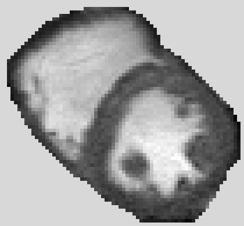
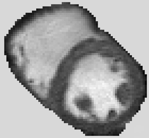
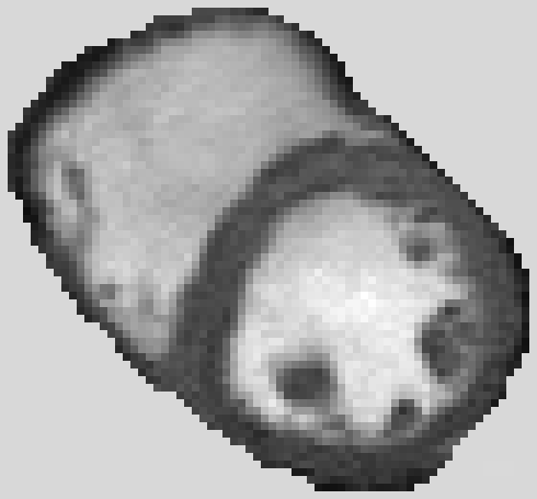
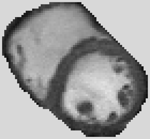
$t=0$	$t=\frac{1}{3}$	$t=\frac{2}{3}$	$t=1$
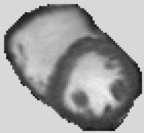
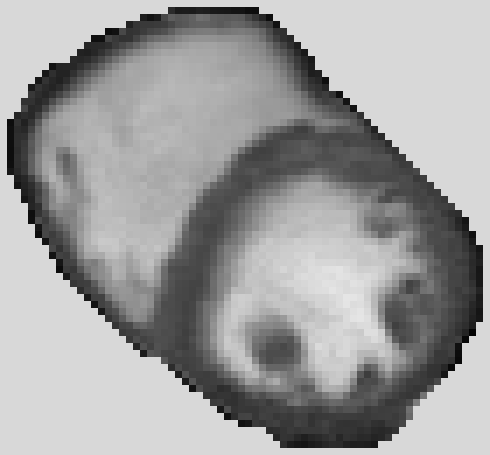
real image	transport image	transport image	real image

Figure 1: Density evolution between two non-convex, differing compact supports. Left and right input images ($t$=0 and $t$=1) show the starting and ending densities and supports (gray background does not represent any density value and has no effect on the computations), while the middle images (bottom) represent transported densities and supports computed at equally spaced intermediate times (with the actual measured cardiac images at corresponding times shown along the top row for comparison).

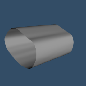
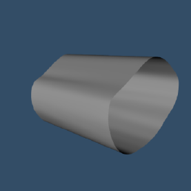
Figure 2: Two rendered viewpoints of the hypersurface ${\bf\Gamma}$ which models/constrains the dynamic support from $t$=0 to $t$=1.

In this first example we tackle the problem of interpolating between cardiac images captured at two different moments within the heart beat cycle shown on the left and the right in Figure 1 Notice that both cell boundaries represent non-convex shapes with several small concavities. We also see structures of interest inside the ventricle (papillary muscle cross sections) which not only move and deform along with the rest of the image, but which also change in their topological appearance. At a coarse scale, the boundary shapes appear to be similar, but detailed inspection reveals that finer scale protrusions and intrusions around the boundary differ, especially the concavity along the upper right edge of the left image which disappears in the right image. Nevertheless, both boundaries exhibit a matching simple topology, which we would like to preserve when morphing one into the other. Numerically, this can be challenging without an explicit model of the support boundary, making it difficult to guarantee that small scale protrusions don’t break off during transport to yield transitional topological changes.

Using these two cardiac images as the starting and ending densities at time $t=0$ and $t=1$ respectively, we solve the compact optimal transport problem with the variational approach outlined in this paper, using a 3D space-time grid for the solenoidal vector field ${\bf W}$ with 64 temporal slices, each of size 128x128 (same resolution as the two input images). A matching level set grid $\Psi$ is used to represent the spatiotemporal support as the set $\Psi<0$. We see the density (temporal component of ${\bf W}$) in Figure 1 at equally space intervals along the computed transport. We can see this more explicitly by visualizing the entire swept-out hypersurface ${\bf\Gamma}$ (the portion of the spatiotemporal support boundary strictly between 0 and 1) in Figure 2. This is very easily rendered as the zero level set of $\Psi$ and clearly reveals a smooth homotopy connecting the two end curves, one exposed within the top rendering and the other within the bottom).

4.2 Optimal transport with spatiotemporal support constraints

This next experiment illustrates through and intuitive toy-example an important and useful extension to the class of optimal transport problems which, to the best of our knowledge, is not accommodated by prior art, but is easily handled within the methodology outlined here. Namely, how might one compute the optimal transport between densities subject to constraints imposed on where (and possibly even when) mass is allowed or not allowed to move along the way?

4.2.1 Known initial and final densities with intermediate support constraints

We can easily motivate the utility of such constraints if we go back to the classic problem posed by Gaspard Monge. In formulating the problem to optimally move a pile of dirt from one place to another, no constraints were imposed on the path taken by each portion of moved dirt. While the unconstrained optimal solution may yield a realistic and realizable transport strategy in several practical circumstances, this cannot always be guaranteed. For example, suppose the task is to move a pile of dirt across a limited number of bridges to the other side of a river. The unconstrained solution could easily yield an impractical transport strategy which involves crossing open portions of the river. A related larger scale problem might involve planning the motion of massive numbers of land troops distributed over a set of territories to another set of territories taking into account geographical barriers such as mountains and bodies of water as well as political barriers which would render certain intermediate territories out of bounds.

Even when the topology of the desired transport is known, optimization subject to geometric constraints can still be nontrivial. For example, transporting a single pile of dirt across a single bridge which is narrower than the base of the pile is already an interesting problem. The unconstrained optimal transport will likely want to move some portion of dirt outside the confines of the bridge. Should all of that excess dirt simply be re-routed and accumulated along the closest edge of the bridge, or should some of it be moved more centrally inside the bridge, which makes the trajectory deviate even further from the unconstrained optimum but attenuates an otherwise massive spike in density along the edge? Clearly there is a trade off that is not easily intuited directly from the unconstrained solution.

These types of constraints are easily imposed using the variational framework presented in this paper due to the explicit representation and separate-yet-coupled evolution of the support boundary. So long as we choose an initial spatiotemporal support that satisfies the provided set of spatiotemporal constraints, the calculated gradient descent evolution of the resulting spatiotemporal hypersurface can simply be set to zero locally wherever its application would otherwise violate the constraints.

4.2.2 Unknown final density but with known support

Figure 3: Example of optimal transport with spatiotemporal support constraints. Mass is evacuated from the center of a disk with uniform initial density of 3.0 (appears as dark-gray/almost-black in the top-left frame), while constrained to remain inside the disk. The optimal evacuation strategy is computed by solving the optimal transport problem between the initial uniform density on the disk back to itself (normally the trivial transport of zero) but imposing a hole in the spatiotemporal support at $t$=$\frac{1}{2}$. Mass therefore evacuates the hole from $t$=0 to $t$=$\frac{1}{2}$ (shown above) and refills the hole from $t$=$\frac{1}{2}$ to $t$=1 (reverse of above).

Another extension of problems that are easily accommodated by this coupled variational approach include scenarios where the support of the target density is given but the target density itself is unknown (and therefore part of the optimization). Such a problem can easily be transformed into the problem of a known final density with intermediate constraints on the support by treating the desired final density as the halfway point ($t=\frac{1}{2}$) in transporting the initial density at $t=0$ back to itself again at $t=1$. In this way, the desired final support becomes a constraint on the intermediate support instead. Optimization of this reconfigured problem will yield both a forward copy (from $t=0$ to $t=\frac{1}{2}$) and a backward copy (from $t=\frac{1}{2}$ to $t=1$) of the optimal transport for the original problem as well as the optimal target density itself at $t=\frac{1}{2}$. As such, from an implementation standpoint, this class of problems can be handled the same way as the class of problems just described above.

A practical application for this form of constrained optimal transport would be to compute the most efficient evacuation strategy to clearing mass out of a given sub-region while keeping it within a larger encompassing region that already contains pre-existing mass. In this case we know the initial density and support, and we know the final support, simply the initial support minus the sub-region to be evacuated, but we don’t know or otherwise want to constrain the resulting new density within the now reduced support. We therefore seek the least costly way (according to the Wasserstein metric) to redistribute the mass originally contained within the subregion into its surrounding, already occupied neighborhood. Such a problem may arise, for example, when seeking to clear extensive zones of all materials and/or personnel while keeping them within the confines of larger zones whose occupants are free to be internally relocated if needed.

We illustrate precisely this scenario with an intuitive toy-problem in Figure 3. We start with uniformly distributed mass at $t=0$ with density 3.0 across a disk representing the global confines. In turn, we define the target distribution at $t=1$ to be the same, but impose a hole in the intermediate support at $t=\frac{1}{2}$ within the center of the disk. Solving the constrained optimal transport problem between these matching uniform distributions causes the initially filled hole to be evacuated from $t=0$ to $t=\frac{1}{2}$, as illustrated from left-to-right and top-to-bottom in Figure 3, and then to be refilled from $t=\frac{1}{2}$ to $t=1$, as also illustrated in Figure 3 when read in reverse. The optimal redistribution of mass is attained at $t=\frac{1}{2}$ and is displayed in grayscale at the end of the figure.

Even in this simplest illustrative example with constant density and maximal symmetry, it is by no means intuitively obvious how far away mass should be displaced from the hole boundary compared to how much it should be allowed to accumulate along the boundary. In fact, the density would become infinite if the evacuated mass were to remain strictly along the boundary. To get a better sense of where displaced mass accumulates upon preexisting mass, we show the net density change in Figure 4 (left side) which attains a maximum rise of 2.3 all around the boundary of the evacuated hole and gradually rolls off further outward.

We can make this toy problem even more interesting by evacuating mass near the boundary of the disk rather than its center. Looking at the resulting net density increase in Figure 4 (right side), we can make several observations. First, as expected, the redistribution is no longer symmetric. The symmetry is broken two different ways. First, the rise in density is much higher (3.0, a full 100% jump) along the bottom border of the hole compared to the top border. This is unsurprising since there is not as much room to move away from the hole, and so the same amount of evacuated mass distributed over a thinner local neighborhood must necessarily result in a larger accumulated density.

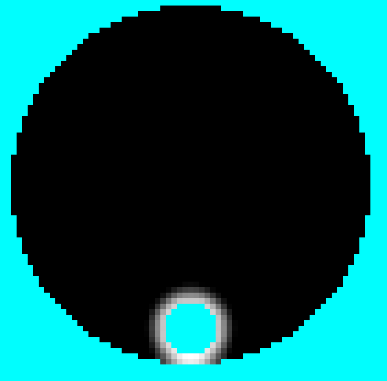
Evacuated mass from disk center	Evacuated mass near disk edge
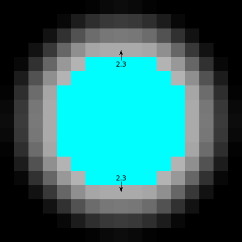
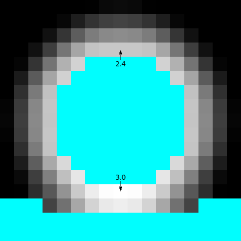
Close-up: symmetric increase	Close-up: nonsymmetric increase

Figure 4: Optimized mass evacuation from two different locations. Both cases begin with uniform mass density (3.0) over the disk then evacuate a hole. Accumulated density results wherever mass gets relocated (see previous figure). Final net accumulation is shown here as the rise in density. When the hole is perfectly centered (left), evacuated mass gets redistributed symmetrically with a peak density rise of 2.3 (77%). Non-symmetric restribution produces a peak rise of 3.0 when the hole is created near the boundary (right).

However, we also notice that the density jump near the top of the hole (2.4), while lower than the bottom, still exceeds the symmetric jump (2.3) when the hole was centered inside the disk. This differential grows as we travel along the border of the hole toward the bottom. This means that some of the mass within the lower half of the hole, which was all evacuated downward from the centered hole, actually got evacuated upward from the hole near the boundary of the confining domain. As such, at least two interesting interplays are relevant in this optimization. First, as in the symmetric case, how far away should mass be displaced away from borders versus accumulated along borders? Second, when displacement distances are limited, what is the right trade-off between higher accumulation at nearby borders versus more costly redirection toward farther borders of the region to be evacuated? These considerations are both naturally handled by this coupled variational framework.

5 Appendices

5.1 Detailed first variation and gradient calculation

We first note that a variation of ${\bf W}$ yields a variation of ${\bf V}$ which is orthogonal to ${\bf W}$ itself. This may be demonstrated directly using the expression (17) as follows.

$$\delta{\bf V} =\left(\frac{\delta{\bf W}}{\left({\bf W}\cdot{\bf e}_{0}\right)}-\frac{{\bf W}}{\left({\bf W}\cdot{\bf e}_{0}\right)^{2}}\left(\delta{\bf W}\cdot{\bf e}_{0}\right)\right)-\left(\frac{\delta{\bf W}\cdot{\bf W}}{\left({\bf W}\cdot{\bf e}_{0}\right)^{2}}-\frac{{\bf W}\cdot{\bf W}}{\left({\bf W}\cdot{\bf e}_{0}\right)^{3}}\left(\delta{\bf W}\cdot{\bf e}_{0}\right)\right){\bf e}_{0}$$

$${\bf W}\cdot\delta{\bf V} =\underbrace{\left(\frac{\delta{\bf W}\cdot{\bf W}}{\left({\bf W}\cdot{\bf e}_{0}\right)}-\frac{{\bf W}\cdot{\bf W}}{\left({\bf W}\cdot{\bf e}_{0}\right)^{2}}\left(\delta{\bf W}\cdot{\bf e}_{0}\right)\right)-\left(\frac{\delta{\bf W}\cdot{\bf W}}{\left({\bf W}\cdot{\bf e}_{0}\right)}-\frac{{\bf W}\cdot{\bf W}}{\left({\bf W}\cdot{\bf e}_{0}\right)^{2}}\left(\delta{\bf W}\cdot{\bf e}_{0}\right)\right)}_{\mbox{terms cancel}}=0$$

Using Lagrange multipliers to incorporate the mass preservation constraints we write the energy as

$$E({\bf W},{\bf\Gamma},\lambda,\alpha)=\int_{{\bf\Omega}}{\bf W}\cdot{\bf V}\,+\lambda\,\nabla\cdot{\bf W}\,d{\bf X}+\int_{{\bf\Gamma}}\alpha{\bf W}\cdot{\bf N}\,dS+\int_{{\bf\Gamma}_{0}}\alpha\left(\overbrace{{\bf W}\cdot{\bf N}}^{-{\bf W}\cdot{\bf{\bf e}_{0}}}+\rho_{0}\right)\,dS+\int_{{\bf\Gamma}_{1}}\alpha\left(\overbrace{{\bf W}\cdot{\bf N}}^{{\bf W}\cdot{\bf e}_{0}}-\rho_{1}\right)\,dS$$

and compute its first variation as follows.

$$\delta E= \int_{{\bf\Omega}}\delta{\bf W}\cdot{\bf V}+\underbrace{{\bf W}\cdot\delta{\bf V}}_{0}+\lambda\nabla\cdot\delta{\bf W}+\delta\lambda\,\nabla\cdot{\bf W}\;d{\bf X}+\int_{{\bf\Gamma}}\left({\bf W}\cdot{\bf V}+\lambda\nabla\cdot{\bf W}\right)\delta{\bf\Gamma}\cdot{\bf N}\,dS$$

$$+\int_{{\bf\Gamma}}\delta\alpha\,{\bf W}\cdot{\bf N}+\alpha\,\delta{\bf W}\cdot{\bf N}\,dS+\int_{{\bf\Gamma}}\left(\nabla_{S}\alpha\cdot{\bf W}+\alpha\nabla\cdot{\bf W}\right)\delta{\bf\Gamma}\cdot{\bf N}\,dS$$

$$-\int_{{\bf\Gamma}_{0}}\delta\alpha\left({\bf W}\cdot{\bf e}_{0}-\rho_{0}\right)+\alpha\,\delta{\bf W}\cdot{\bf e}_{0}\,dS+\int_{{\bf\Gamma}_{1}}\delta\alpha\left({\bf W}\cdot{\bf e}_{0}-\rho_{1}\right)+\alpha\,\delta{\bf W}\cdot{\bf e}_{0}\,dS$$

$$= \int_{{\bf\Omega}}\delta{\bf W}\cdot\left({\bf V}-\nabla\lambda\right)+\delta\lambda\,\nabla\cdot{\bf W}\;d{\bf X}+\int_{\partial{\bf\Omega}}\lambda\,\delta{\bf W}\cdot{\bf N}\,dS$$

$$+\int_{{\bf\Gamma}}\delta\alpha\,{\bf W}\cdot{\bf N}+\alpha\,\delta{\bf W}\cdot{\bf N}+\left({\bf W}\cdot\left({\bf V}+\nabla_{S}\alpha\right)+\left(\lambda+\alpha\right)\nabla\cdot{\bf W}\right)\delta{\bf\Gamma}\cdot{\bf N}\,dS$$

$$-\int_{{\bf\Gamma}_{0}}\delta\alpha\left({\bf W}\cdot{\bf e}_{0}-\rho_{0}\right)+\alpha\,\delta{\bf W}\cdot{\bf e}_{0}\,dS+\int_{{\bf\Gamma}_{1}}\delta\alpha\left({\bf W}\cdot{\bf e}_{0}-\rho_{1}\right)+\alpha\,\delta{\bf W}\cdot{\bf e}_{0}\,dS$$

$$= \int_{{\bf\Omega}}\delta{\bf W}\cdot\left({\bf V}-\nabla\lambda\right)+\delta\lambda\,\nabla\cdot{\bf W}\;d{\bf X}$$

$$+\int_{{\bf\Gamma}}\delta\alpha\,{\bf W}\cdot{\bf N}+\left(\lambda+\alpha\right)\,\delta{\bf W}\cdot{\bf N}+\left({\bf W}\cdot\left({\bf V}+\nabla_{S}\alpha\right)+\left(\lambda+\alpha\right)\nabla\cdot{\bf W}\right)\delta{\bf\Gamma}\cdot{\bf N}\,dS$$

$$-\int_{{\bf\Gamma}_{0}}\delta\alpha\left({\bf W}\cdot{\bf e}_{0}-\rho_{0}\right)+\left(\lambda+\alpha\right)\,\delta{\bf W}\cdot{\bf e}_{0}\,dS+\int_{{\bf\Gamma}_{1}}\delta\alpha\left({\bf W}\cdot{\bf e}_{0}-\rho_{1}\right)+\left(\lambda+\alpha\right)\,\delta{\bf W}\cdot{\bf e}_{0}\,dS$$

Plugging in the mass conversation constraints eliminates the dependence on $\delta\lambda$ and $\delta\alpha$ yielding the simpler expression

$$\delta E= \int_{{\bf\Omega}}\delta{\bf W}\cdot\left({\bf V}-\nabla\lambda\right)\;d{\bf X}+\int_{{\bf\Gamma}}\left(\lambda+\alpha\right)\,\delta{\bf W}\cdot{\bf N}+{\bf W}\cdot\left({\bf V}+\nabla_{S}\alpha\right)\delta{\bf\Gamma}\cdot{\bf N}\,dS$$

$$-\int_{{\bf\Gamma}_{0}}\left(\lambda+\alpha\right)\,\delta{\bf W}\cdot{\bf e}_{0}\,dS+\int_{{\bf\Gamma}_{1}}\left(\lambda+\alpha\right)\,\delta{\bf W}\cdot{\bf e}_{0}\,dS$$

Now apply the Helmholtz decomposition

$${\bf V}={\bf V}^{\parallel}+{\bf V}^{\perp}$$

where

$${\bf V}^{\parallel} =\nabla\phi$$

$${\bf V}^{\perp} ={\bf V}-\nabla\phi$$

$$\Delta\phi =\nabla\cdot{\bf V}\;\mbox{inside }{\bf\Omega}\quad\left(\mbox{$\therefore\nabla\cdot{\bf V}^{\perp}=0$}\right)$$

$$\nabla\phi\cdot\underbrace{{\bf N}}_{-{\bf e}_{0}} ={\bf V}\cdot{\bf N}\;\mbox{along }{\bf\Gamma}_{0}\quad\left(\mbox{$\therefore{\bf V}^{\perp}\cdot{\bf e}_{0}=0$}\right)$$

$$\nabla\phi\cdot\underbrace{{\bf N}}_{+{\bf e}_{0}} ={\bf V}\cdot{\bf N}\;\mbox{along }{\bf\Gamma}_{1}\quad\left(\mbox{$\therefore{\bf V}^{\perp}\cdot{\bf e}_{0}=0$}\right)$$

(note that the decomposition still depends upon the boundary condition for $\phi$ along ${\bf\Gamma}$). We choose $\delta{\bf W}={\bf V}^{\perp}$ to maintain the internal mass conservation constraint $\nabla\cdot{\bf W}=0$ as well as the flux constraints along ${\bf\Gamma}_{0}$ and ${\bf\Gamma}_{1}$. This eliminates the dependencies upon $\lambda$ everywhere and upon $\alpha$ along the temporal faces ${\bf\Gamma}_{0}$ and ${\bf\Gamma}_{1}$.

$$\delta E(\phi)= \int_{{\bf\Omega}}\|{\bf V}^{\perp}\|^{2}+{\bf V}^{\perp}\cdot{\bf V}^{\parallel}-{\bf V}^{\perp}\cdot\nabla\lambda\;d{\bf X}+\int_{{\bf\Gamma}}\left(\lambda+\alpha\right)\,{\bf V}^{\perp}\cdot{\bf{\bf N}}+{\bf W}\cdot\left({\bf V}+\nabla_{S}\alpha\right)\delta{\bf\Gamma}\cdot{\bf N}\,dS$$

$$-\int_{{\bf\Gamma}_{0}}\left(\lambda+\alpha\right)\,\underbrace{{\bf V}^{\perp}\cdot{\bf e}_{0}}_{0}\,dS+\int_{{\bf\Gamma}_{1}}\left(\lambda+\alpha\right)\,\underbrace{{\bf V}^{\perp}\cdot{\bf e}_{0}}_{0}\,dS$$

$$= \int_{{\bf\Omega}}\|{\bf V}^{\perp}\|^{2}+{\bf V}^{\perp}\cdot\nabla\phi+\lambda\underbrace{\nabla\cdot{\bf V}^{\perp}}_{0}\;d{\bf X}+\int_{{\bf\Gamma}}\alpha\,{\bf V}^{\perp}\cdot{\bf{\bf N}}+{\bf W}\cdot\left({\bf V}+\nabla_{S}\alpha\right)\delta{\bf\Gamma}\cdot{\bf N}\,dS$$

$$= \int_{{\bf\Omega}}\|{\bf V}^{\perp}\|^{2}-\phi\underbrace{\nabla\cdot{\bf V}^{\perp}}_{0}\;d{\bf X}+\int_{{\bf\Gamma}}\left(\phi+\alpha\right)\,{\bf V}^{\perp}\cdot{\bf{\bf N}}+{\bf W}\cdot\left({\bf V}+\nabla_{S}\alpha\right)\delta{\bf\Gamma}\cdot{\bf N}\,dS$$

$$= \int_{{\bf\Omega}}\|{\bf V}^{\perp}\|^{2}\;d{\bf X}+\int_{{\bf\Gamma}}\left(\phi+\alpha\right)\,{\bf V}^{\perp}\cdot{\bf{\bf N}}+{\bf W}\cdot\left({\bf V}+\nabla_{S}\alpha\right)\delta{\bf\Gamma}\cdot{\bf N}\,dS$$

$$= \int_{{\bf\Omega}}\|{\bf V}-\nabla\phi\|^{2}\;d{\bf X}+\int_{{\bf\Gamma}}\left(\phi+\alpha\right)\,\left({\bf V}-\nabla\phi\right)\cdot{\bf{\bf N}}+{\bf W}\cdot\left({\bf V}+\nabla_{S}\alpha\right)\delta{\bf\Gamma}\cdot{\bf N}\,dS$$

5.2 Coupled boundary and flux perturbations

To maintain the vanishing flux constraint ${\bf W}\cdot{\bf N}=0$ along hypersurface ${\bf\Gamma}$ portion of the support boundary $\partial{\bf\Omega}$, the normal perturbation $\delta{\bf\Gamma}\cdot{\bf N}$ of the boundary itself and the normal component of the solenoidal field perturbation $\delta{\bf W}\cdot{\bf N}$ cannot be applied independently but are coupled. This should not be surprising because the field ${\bf W}$ defines the transport which, by virtue of determining the density evolution, also determines the evolution of its support. To determine the resulting coupling between a support perturbation $\delta{\bf\Gamma}\cdot{\bf N}$ and the matching flux perturbation $\delta{\bf W}\cdot{\bf N}$, we differentiate the following constraint along the swept-out hypersurface

$${\bf W}({\bf{\bf\Gamma}}(s))\cdot{\bf N}(s)=0$$ (37)

where

$$s=(s_{1},\ldots,s_{n})$$

denotes isothermal coordinates aligned with the principal directions ${\bf T}_{1},\ldots,{\bf T}_{n}$ (unit tangent vectors) of the hypersurface. We choose this parameterization for the convenient property that geodesic torsions vanish along principal directions, and therefore

$$\frac{\partial{\bf T}_{j}}{\partial s_{i}}=\begin{cases}\kappa_{i}{\bf N},&i=j\\ 0,&i\neq j\end{cases}$$

were $\kappa_{i}$ denotes the principle curvature. We now expand

$$\delta({\bf W}\cdot{\bf N})=\left(\frac{\partial{\bf W}}{\partial{\bf X}}\delta{\bf\Gamma}+\delta{\bf W}\right)\cdot{\bf N}+{\bf W}\cdot\delta{\bf N}=0$$

to obtain

$$\delta{\bf W}\cdot{\bf N}= -{\bf N}^{T}\frac{\partial{\bf W}}{\partial{\bf X}}\delta{\bf\Gamma}-{\bf W}\cdot\delta{\bf N}$$

$$= \underbrace{-\left({\bf N}^{T}\frac{\partial{\bf W}}{\partial{\bf X}}{\bf N}\right)\delta{\bf\Gamma}\cdot{\bf N}-\sum_{i=1}^{n}\left({\bf N}^{T}\frac{\partial{\bf W}}{\partial{\bf X}}{\bf T}_{i}\right)\delta{\bf\Gamma}\cdot{\bf T}_{i}}_{{\bf\mbox{orthogonal components of }-{\bf N}^{T}\frac{\partial{\bf W}}{\partial{\bf X}}}\delta{\bf\Gamma}}-{\bf W}\cdot\underbrace{\left(\sum_{i=1}^{n}-{\bf T}_{i}\left(\frac{\partial(\delta{\bf\Gamma})}{\partial s_{i}}\cdot{\bf N}\right)\right)}_{\delta{\bf N}}$$

$$= \left(\overbrace{\nabla\cdot{\bf W}}^{0}-{\bf N}^{T}\frac{\partial{\bf W}}{\partial{\bf X}}{\bf N}\right)\delta{\bf\Gamma}\cdot{\bf N}-\sum_{i=1}^{n}\left({\bf N}^{T}\frac{\partial{\bf W}}{\partial{\bf X}}{\bf T}_{i}\right)\delta{\bf\Gamma}\cdot{\bf T}_{i}+\sum_{i=1}^{n}{\bf W}\cdot{\bf T}_{i}\left(\frac{\partial(\delta{\bf\Gamma})}{\partial s_{i}}\cdot{\bf N}\right)$$

$$= \left(\sum_{i=1}^{n}{\bf T}_{i}^{T}\frac{\partial{\bf W}}{\partial{\bf X}}{\bf T}_{i}\right)\delta{\bf\Gamma}\cdot{\bf N}-\sum_{i=1}^{n}\left({\bf N}^{T}\frac{\partial{\bf W}}{\partial{\bf X}}{\bf T}_{i}\right)\delta{\bf\Gamma}\cdot{\bf T}_{i}+\sum_{i=1}^{n}\left(\frac{\partial(\delta{\bf\Gamma})}{\partial s_{i}}\cdot{\bf N}\right)\left({\bf W}\cdot{\bf T}_{i}\right)$$

$$= \left(\sum_{i=1}^{n}{\bf T}_{i}^{T}\overbrace{\frac{\partial{\bf W}}{\partial{\bf X}}{\bf T}_{i}}^{\frac{\partial{\bf W}}{\partial s_{i}}}+\overbrace{{\bf W}\cdot\frac{\partial{\bf T}_{i}}{\partial s_{i}}}^{\kappa_{i}{\bf W}\cdot{\bf N}=0}\right)\delta{\bf\Gamma}\cdot{\bf N}-\sum_{i=1}^{n}\left({\bf N}^{T}\frac{\partial{\bf W}}{\partial{\bf X}}{\bf T}_{i}\right)\delta{\bf\Gamma}\cdot{\bf T}_{i}+\sum_{i=1}^{n}\left(\frac{\partial(\delta{\bf\Gamma})}{\partial s_{i}}\cdot{\bf N}\right)\left({\bf W}\cdot{\bf T}_{i}\right)$$

$$= \sum_{i=1}^{n}\frac{\partial}{\partial s_{i}}\left({\bf W}\cdot{\bf T}_{i}\right)\delta{\bf\Gamma}\cdot{\bf N}-\left({\bf N}^{T}\frac{\partial{\bf W}}{\partial{\bf X}}{\bf T}_{i}\right)\delta{\bf\Gamma}\cdot{\bf T}_{i}+\left(\frac{\partial(\delta{\bf\Gamma})}{\partial s_{i}}\cdot{\bf N}\right)\left({\bf W}\cdot{\bf T}_{i}\right)$$

Differentiating the vanishing flux condition (37) along each principal direction yields

$$\frac{\partial}{\partial s_{i}}({\bf W}\cdot{\bf N})=\left(\frac{\partial{\bf W}}{\partial{\bf X}}{\bf T}_{i}\right)\cdot{\bf N}-{\bf W}\cdot\kappa_{i}{\bf T}=0$$

allowing us to substitute

$${\bf N}^{T}\frac{\partial{\bf W}}{\partial{\bf X}}{\bf T}_{i}={\bf W}\cdot\kappa_{i}{\bf T}_{i}$$

into our previous expression and to continue as follows

$$\delta{\bf W}\cdot{\bf N}= \sum_{i=1}^{n}\frac{\partial}{\partial s_{i}}\left({\bf W}\cdot{\bf T}_{i}\right)\delta{\bf\Gamma}\cdot{\bf N}-\left({\bf W}\cdot\kappa_{i}{\bf T}_{i}\right)\delta{\bf\Gamma}\cdot{\bf T}_{i}+\left(\frac{\partial(\delta{\bf\Gamma})}{\partial s_{i}}\cdot{\bf N}\right)\left({\bf W}\cdot{\bf T}_{i}\right)$$

$$= \sum_{i=1}^{n}\frac{\partial}{\partial s_{i}}\left({\bf W}\cdot{\bf T}_{i}\right)\delta{\bf\Gamma}\cdot{\bf N}-\left({\bf W}\cdot\kappa_{i}{\bf T}_{i}\right)\delta{\bf\Gamma}\cdot{\bf T}_{i}+\frac{\partial(\sum_{j=1}^{n}\left(\delta{\bf\Gamma}\cdot{\bf T}_{j}\right){\bf T}_{j}+\left(\delta{\bf\Gamma}\cdot{\bf N}\right){\bf N})}{\partial s_{i}}\cdot{\bf N}\left({\bf W}\cdot{\bf T}_{i}\right)$$

$$= \sum_{i=1}^{n}\frac{\partial}{\partial s_{i}}\left({\bf W}\cdot{\bf T}_{i}\right)\delta{\bf\Gamma}\cdot{\bf N}-\kappa_{i}\left({\bf W}\cdot{\bf T}_{i}\right)\delta{\bf\Gamma}\cdot{\bf T}_{i}+\left(\sum_{j\neq i}\left(\delta{\bf\Gamma}\cdot{\bf T}_{j}\right)\underbrace{\frac{\partial{\bf T}_{j}}{\partial s_{i}}}_{0}+\left(\delta{\bf\Gamma}\cdot{\bf T}_{i}\right)\underbrace{\frac{\partial{\bf T}_{i}}{\partial s_{i}}}_{\kappa_{i}}+\frac{\partial}{\partial s_{i}}\left(\delta{\bf\Gamma}\cdot{\bf N}\right)\right)\left({\bf W}\cdot{\bf T}_{i}\right)$$

$$= \sum_{i=1}^{n}\frac{\partial}{\partial s_{i}}\left({\bf W}\cdot{\bf T}_{i}\right)\delta{\bf\Gamma}\cdot{\bf N}+\frac{\partial}{\partial s_{i}}\left(\delta{\bf\Gamma}\cdot{\bf N}\right)\left({\bf W}\cdot{\bf T}_{i}\right)$$

yielding the final expression for the coupling between $\delta{\bf W}\cdot{\bf N}$ and $\delta{\bf\Gamma}\cdot{\bf N}$.

$$\delta{\bf W}\cdot{\bf N}=\sum_{i=1}^{n}\frac{\partial}{\partial s_{i}}\Bigl{(}({\bf W}\cdot{\bf T}_{i})(\delta{\bf\Gamma}\cdot{\bf N})\Bigr{)}$$

It is generally difficult to invert this expression to express the boundary perturbation $\delta{\bf\Gamma}\cdot{\bf N}$ as a function of the flux perturbation $\delta{\bf W}\cdot{\bf N}$. However, in the special case of zero flux perturbation ${\bf\delta{\bf W}\cdot{\bf N}=}0$, we obtain

$$\sum_{i=1}^{n}\frac{\partial}{\partial s_{i}}\Bigl{(}({\bf W}\cdot{\bf T}_{i})(\delta{\bf\Gamma}\cdot{\bf N})\Bigr{)}=0$$

which, combined with the constraint that $\delta{\bf\Gamma}\cdot{\bf N}=0$ along the temporal boundaries of ${\bf\Gamma}$ at $t=0$ and at $t=1$, only admits the solution $\delta{\bf\Gamma}\cdot{\bf N}=0$ along the entirety of the hypersurface ${\bf\Gamma}$. As such, a vanishing flux perturbation implies a vanishing perturbation of the support boundary. The converse is also trivially demonstrated directly through equation (37).

5.3 Gradient descent step size

Maximum allowed step factor

Since any choice of step factor $\gamma_{k}$ in (34) maintains the solenoidal constraint and boundary flux conditions for ${\bf W}_{k+1}$, we enforce the constraint $\rho_{k+1}(\text{{\bf X}})>0$ for all ${\bf X}\in{\bf\Omega}$ to determine the upper limit for the allowable step factor $\gamma_{k}$.

$$0<\rho_{k+1}={\bf W}_{k+1}\cdot{\bf e}_{0}=\left({\bf W}_{k}+\gamma_{k}\underbrace{\delta{\bf W}_{k}}_{-{\bf V}_{k}^{\perp}}\right)\cdot{\bf e}_{0}={\bf\rho}_{k}+\,\gamma_{k}\delta\rho_{k}$$

Notice that this inequality is satisfied for arbitrarily large $\gamma_{k}$ whenever $\delta\rho_{k}\geq 0$ and so an upper bound needs to be considered only in cases where $\delta\rho_{k}({\bf X})<0$ for some ${\bf X}\in{\bf\Omega}$. Accordingly, if we denote the set

$${\bf\Omega}^{-}=\left\{{\bf X}\in{\bf\Omega}\;|\;\delta\rho_{k}<0\right\}$$

we may formulate the following strict upper bound for $\gamma_{k}$.

$$\gamma_{k,\max}=\begin{cases}\min\limits_{{\bf\Omega}^{-}}\left(-{\displaystyle\frac{{\bf\rho}_{k}}{\delta\rho_{k}}}\right),&{\bf\Omega}^{-}\neq\emptyset\\ \infty,&{\bf\Omega}^{-}=\emptyset\end{cases}$$

A numerically robust way to compute $y_{k,\max}$ while avoiding numerical overflow is to start with an exceedingly large estimate and then loop through the points ${\bf X}\in{\bf\Omega}$, checking for the condition $\gamma_{k,\max}\,\delta\rho_{k}<-\rho_{k}$. Whenever the condition is detected, the value of $y_{k,\max}$ should be replaced by $-\frac{{\bf\rho}_{k}}{\delta\rho_{k}}$ at the detected location ${\bf X}$. Since this condition will never be satisfied for points outside of the set ${\bf\Omega}^{+}$, there is no need test whether ${\bf X}\in{\bf\Omega}^{-}$ beforehand.

Some preliminary calculations

Using the dot notation for the derivative with respect to $\gamma_{k}$ we begin with a few preliminary calculations as follows. The last two dot product expressions will be useful in formulating the Newton update.

$${\bf W}_{k+1} ={\bf W}_{k}+\gamma_{k}\delta{\bf W}_{k}$$

$$\dot{{\bf W}}_{k+1} =\delta{\bf W}_{k}$$

$${\bf V}_{k+1} ={\bf U}_{k+1}-\frac{1}{2}\left({\bf U}_{k+1}\cdot{\bf U}_{k+1}+1\right){\bf e}_{0}=\frac{{\bf W}_{k+1}}{{\bf W}_{k+1}\cdot{\bf e}_{0}}-\frac{1}{2}\left(\frac{{\bf W}_{k+1}\cdot{\bf W}_{k+1}}{\left({\bf W}_{k+1}\cdot{\bf e}_{0}\right)^{2}}+1\right){\bf e}_{0}$$

$$\dot{{\bf V}}_{k+1} =\frac{1}{{\bf W}_{k+1}\cdot{\bf e}_{0}}\left(\delta{\bf W}_{k}-\frac{{\bf W}_{k+1}}{{\bf W}_{k+1}\cdot{\bf e}_{0}}\delta{\bf W}_{k}\cdot{\bf e}_{0}-\left(\frac{{\bf W}_{k+1}\cdot\delta{\bf W}_{k}}{{\bf W}_{k+1}\cdot{\bf e}_{0}}-\frac{{\bf W}_{k+1}\cdot{\bf W}_{k+1}}{\left({\bf W}_{k+1}\cdot{\bf e}_{0}\right)^{2}}\delta{\bf W}_{k}\cdot{\bf e}_{0}\right){\bf e}_{0}\right)$$

$${\bf W}_{k+1}\cdot\dot{{\bf V}}_{k+1} =0$$

$$\delta{\bf W}_{k}\cdot\dot{{\bf V}}_{k+1} =\frac{1}{{\bf W}_{k+1}\cdot{\bf e}_{0}}\left(\delta{\bf W}_{k}\cdot\delta{\bf W}_{k}-2\left(\frac{\delta{\bf W}_{k}\cdot{\bf e}_{0}}{{\bf W}_{k+1}\cdot{\bf e}_{0}}\right){\bf W}_{k+1}\cdot\delta{\bf W}_{k}+\left(\frac{\delta{\bf W}_{k}\cdot{\bf e}_{0}}{{\bf W}_{k+1}\cdot{\bf e}_{0}}\right)^{2}{\bf W}_{k+1}\cdot{\bf W}_{k+1}\right)$$

$$=\frac{1}{{\bf W}_{k+1}\cdot{\bf e}_{0}}\left\|\delta{\bf W}_{k}-\frac{\delta{\bf W}_{k}\cdot{\bf e}_{0}}{{\bf W}_{k+1}\cdot{\bf e}_{0}}{\bf W}_{k+1}\right\|^{2}=\frac{1}{{\bf W}_{k+1}\cdot{\bf e}_{0}}\left\|\underbrace{\delta{\bf W}_{k}-\left(\delta{\bf W}_{k}\cdot{\bf e}_{0}\right){\bf U}_{k+1}}_{{\bf e}_{0}\mbox{-components cancel}}\right\|^{2}$$

$$=\frac{\left\|\delta{\rm p}_{k}-\delta\rho_{k}v_{k+1}\right\|^{2}}{\rho_{k+1}}$$

where $\delta{\rm p}_{k}$ (momentum increment) denotes the spatial components of $\delta{\bf W}_{k}$ and where $\delta\rho_{k}$ (mass increment) denotes its temporal component

$$\delta{\bf W}_{k}=(\delta\rho_{k},\delta{\rm p}_{k})$$

Optimal step factor

We may employ Newton’s method to maximize the descent taken by the single step 34. To do so, we first derive expressions for the first and second derivatives of the updated energy $E_{k+1}$ as a function of $\gamma_{k}$ (exploiting the preliminary calculations listed above).

$$E_{k+1}(\gamma_{k}) =\int_{{\bf\Omega}}{\bf W}_{k+1}(\gamma_{k})\cdot{\bf V}_{k+1}(\gamma_{k})\,d{\bf X}$$

$$\dot{E}_{k+1}(\gamma_{k}) =\int_{{\bf\Omega}}{\bf\dot{W}}_{k+1}(\gamma_{k})\cdot{\bf V}_{k+1}(\gamma_{k})+\underbrace{{\bf W}_{k+1}(\gamma_{k})\cdot\dot{{\bf V}}_{k+1}(\gamma_{k})}_{0}\,d{\bf X}=\int_{{\bf\Omega}}\delta{\bf W}_{k}\cdot{\bf V}_{k+1}(\gamma_{k})\,d{\bf X}$$

$$\ddot{E}_{k+1}(\gamma_{k}) =\int_{{\bf\Omega}}\delta{\bf W}_{k}\cdot\dot{{\bf V}}_{k+1}(\gamma_{k})\,d{\bf X}=\int_{{\bf\Omega}}\frac{\left\|\delta{\rm p}_{k}-\delta\rho_{k}v_{k+1}\right\|^{2}}{\rho_{k+1}}\,d{\bf X}$$

Notice that

$$\ddot{E}_{k+1}(\gamma_{k}) \geq 0\quad\forall\gamma_{k}$$

$$\dot{E}_{k+1}(0) =\int_{{\bf\Omega}}\underbrace{\delta{\bf W}_{k}}_{-{\bf V}_{k}^{\perp}}\cdot{\bf V}_{k}\,d{\bf X}=\underbrace{-\int_{{\bf\Omega}}{\bf V}_{k}^{\perp}\cdot{\bf V}_{k}\,d{\bf X}=-\int_{{\bf\Omega}}\|{\bf V}_{k}^{\perp}\|^{2}\,d{\bf X}}_{\mbox{by orthogonality of ${\bf V}_{k}^{\perp}$and ${\bf V}_{k}^{\parallel}$}}\leq 0$$

and so, by the first inequality, $E_{k+1}(\gamma_{k})$ is convex with a unique local (i.e. global) minimum which is, by the second inequality, achieved for some $\gamma_{k}\geq 0$. If, in addition,

$$\dot{E}_{k+1}(\gamma_{k,\max})=\int_{{\bf\Omega}}\delta{\bf W}_{k}\cdot{\bf V}_{k+1}(\gamma_{k,\max})\,d{\bf X}\geq 0$$

then we can be apply Newton iterations $\gamma_{k}\to\gamma_{k}-\frac{\dot{E}_{k+1}}{\ddot{E}_{k+1}}$ to solve $\dot{E}_{k+1}(\gamma_{k})=0$ for $\gamma_{k}$ as follows.

Solve: $$\mbox{Poisson equation for $\lambda_{k}$ given }{\bf V}_{k}$$

Initialize: $$\delta{\bf W}_{k}={\bf V}_{k}^{\perp}={\bf V}_{k}-\nabla\lambda_{k}$$

$$\gamma_{k}=0$$

Loop: $${\bf W}_{k+1}={\bf W}_{k}+\gamma_{k}\delta{\bf W}_{k}=(\rho_{k+1},{\rm p}_{k+1})$$

$${\bf V}_{k+1}=\left(-\frac{1}{2}\|v_{k+1}\|^{2}\,,\,v_{k+1}\right)$$

$$\Delta\gamma_{k}=\frac{\dot{E}_{k+1}}{\ddot{E}_{k+1}}=\frac{\int_{{\bf\Omega}}\delta{\bf W}_{k}\cdot{\bf V}_{k+1}\,d{\bf X}}{\int_{{\bf\Omega}}\frac{\left\|\delta\rho_{k}\,v_{k+1}-\delta{\rm p}_{k}\right\|^{2}}{\rho_{k+1}}\,d{\bf X}}$$

$$\gamma_{k}\to\gamma_{k}-\Delta\gamma_{k}\;\left[\mbox{clip if needed so }0\leq\gamma_{k}<\gamma_{k,\max}\right]$$

References

- [1] G. Monge, “Mémoire sur la théorie des déblais et des remblais,” Histoire de l’Académie Royale des Sciences de Paris, 1781.
- [2] L. V. Kantorovich, “On a problem of monge,” CR (Doklady) Acad. Sci. URSS (NS), vol. 3, pp. 225–226, 1948.
- [3] W. Gangbo and R. McCann, “The geometry of optimal transportation,” Acta Mathematica, vol. 177, no. 2, pp. 113–161, 1996.
- [4] C. Villani, Topics in Optimal Transportation. American Mathematical Soc., 2003.
- [5] C. Villani, Optimal Transport: Old and New, vol. 338. Springer Science & Business Media, 2008.
- [6] L. C. Evans and W. Gangbo, “Differential equations methods for the Monge-Kantorovich mass transfer problem,” Memoirs of the American Mathematical Society, vol. 137, no. 653, pp. 0–0, 1999.
- [7] S. T. Rachev and L. Rüschendorf, Mass Transportation Problems: Volume I: Theory. Probability and its Applications, Berlin: Springer, 1998.
- [8] M. Arjovsky, S. Chintala, and L. Bottou, “Wasserstein GAN,” arxiv.org, vol. 1701.07875, 2017.
- [9] E. A. Carlen and J. Maas, “An analog of the 2-Wasserstein metric in non-commutative probability under which the Fermionic Fokker–Planck equation is gradient flow for the entropy,” Communications in Mathematical Physics, vol. 331, no. 3, pp. 887–926, 2014.
- [10] S. Haker, L. Zhu, A. Tannenbaum, and S. Angenent, “Optimal mass transport for registration and warping,” International Journal of Computer Vision, vol. 60, no. 3, pp. 225–240, 2004.
- [11] M. Mittnenzweig and A. Mielke, “An entropic gradient structure for lindblad equations and generic for quantum systems coupled to macroscopic models,” arXiv preprint arXiv:1609.05765, 2016.
- [12] S. T. Rachev and L. Rüschendorf, Mass Transportation Problems: Volumes I and II. Springer Science & Business Media, 1998.
- [13] J. C. Mathews, S. Nadeem, M. Pouryahya, Z. Belkhatir, J. O. Deasy, A. J. Levine, and A. R. Tannenbaum, “Functional network analysis reveals an immune tolerance mechanism in cancer,” Proceedings of the National Academy of Sciences, vol. 117, pp. 16339–16345, jul 2020.
- [14] J.-D. Benamou and Y. Brenier, “A computational fluid mechanics solution to the Monge-Kantorovich mass transfer problem,” Numerische Mathematik, vol. 84, no. 3, pp. 375–393, 2000.
- [15] F. Otto, “The geometry of dissipative evolution equations: the porous medium equation,” Communications in Partial Differential Equations, vol. 26, no. 1-2, pp. 101–174, 2001.
- [16] L. Zhu, Y. Yang, S. Haker, and A. Tannenbaum, “An image morphing technique based on optimal mass preserving mapping,” IEEE Transactions on Image Processing, vol. 16, no. 6, pp. 1481–1495, 2007.
- [17] S. Haker, A. Tannenbaum, and R. Kikinis, “Mass preserving mappings and image registration,” MICCAI, pp. 120–127, 2001.
- [18] S. Osher and R. Fedkiw, Level Set Methods and Dynamic Implicit Surfaces. Springer, 2003.
- [19] J. Sethian, Level Set Methods Fast Marching Methods. Cambridge University Press, 1999.
- [20] G. Sapiro, Geometric Partial Equations and Image Analysis. Cambridge University Press, 2001.
- [21] L. Susskind and A. Friedman, Special Relativity and Classical Field Theory: The Theoretical Minimum. Hachette Book Group, 2017.