Kilonova Detectability with Wide-Field Instruments

Abstract

Kilonovae are ultraviolet, optical, and infrared transients powered by the radioactive decay of heavy elements following a neutron star merger. Joint observations of kilonovae and gravitational waves can offer key constraints on the source of Galactic r-process enrichment, among other astrophysical topics. However, robust constraints on heavy element production requires rapid kilonova detection (within $\sim 1$ day of merger) as well as multi-wavelength observations across multiple epochs. In this study, we quantify the ability of 13 wide field-of-view instruments to detect kilonovae, leveraging a large grid of over 900 radiative transfer simulations with 54 viewing angles per simulation. We consider both current and upcoming instruments, collectively spanning the full kilonova spectrum. The Roman Space Telescope has the highest redshift reach of any instrument in the study, observing kilonovae out to $z\sim 1$ within the first day post-merger. We demonstrate that BlackGEM, DECam, GOTO, the Vera C. Rubin Observatory’s LSST, ULTRASAT, and VISTA can observe some kilonovae out to $z\sim 0.1$ ($\sim$475 Mpc), while DDOTI, MeerLICHT, PRIME, Swift/UVOT, and ZTF are confined to more nearby observations. Furthermore, we provide a framework to infer kilonova ejecta properties following non-detections and explore variation in detectability with these ejecta parameters.

1 Introduction

Neutron star mergers have long been invoked as a cosmic source of heavy elements, produced through rapid neutron capture (r-process) nucleosynthesis (Lattimer & Schramm, 1974; Lattimer et al., 1977; Symbalisty & Schramm, 1982; Eichler et al., 1989; Freiburghaus et al., 1999; Côté et al., 2018). Heavy lanthanides and actinides fuse in material gravitationally unbound during the coalescence of either binary neutron stars (BNS) or neutron star–black hole (NSBH) binaries with near-equal mass ratios (Metzger, 2019). The residual radioactive decay of these r-process elements spurs electromagnetic emission, called a kilonova (Li & Paczyński, 1998; Kulkarni, 2005; Metzger et al., 2010).

Kilonova emission spans ultraviolet, optical, and near-infrared wavelengths (UVOIR), with lower wavelength “blue” emission fading within a day of merger, giving way to “red” emission persisting for over a week. Observations of a kilonova’s rapid evolution can reveal the role of neutron star mergers in Galactic r-process enrichment, while holding promise for additional discoveries in cosmology, nuclear physics, and stellar astrophysics.

Gamma-ray burst emission may also accompany a neutron star merger (Blinnikov et al., 1984; Paczynski, 1986; Eichler et al., 1989; Narayan et al., 1992), with later theories (Popham et al., 1999; Fryer et al., 1999) linking neutron star mergers to short-duration gamma-ray bursts (sGRBs): transient signals with hard gamma-ray emission persisting for less than two seconds (Norris et al., 1984; Kouveliotou et al., 1993). Numerous follow-up observations of sGRBs reveal viable kilonova candidates (Perley et al., 2009; Tanvir et al., 2013; Berger et al., 2013; Yang et al., 2015; Jin et al., 2016; Troja et al., 2018; Gompertz et al., 2018; Ascenzi et al., 2019; Lamb et al., 2019; Troja et al., 2019b; Jin et al., 2020; Rossi et al., 2020; Fong et al., 2021; Rastinejad et al., 2021; O’Connor et al., 2021), strengthening the theorized connection between sGRBs, kilonovae, and neutron star mergers. Astronomers solidified this connection with the joint detection of gravitational-wave (GW) event GW170817 (Abbott et al., 2017c), GRB 170817A (Abbott et al., 2017b; Goldstein et al., 2017; Savchenko et al., 2017), and kilonova AT 2017gfo (Andreoni et al., 2017; Arcavi et al., 2017; Chornock et al., 2017; Coulter et al., 2017; Covino et al., 2017; Cowperthwaite et al., 2017; Drout et al., 2017; Evans et al., 2017; Kasliwal et al., 2017; Lipunov et al., 2017; Nicholl et al., 2017; Pian et al., 2017; Shappee et al., 2017; Smartt et al., 2017; Tanvir et al., 2017; Troja et al., 2017; Utsumi et al., 2017; Valenti et al., 2017). GW170817 also serves as the first GW detection containing a neutron star (Abbott et al., 2017c) and the first multi-messenger detection with GWs (Abbott et al., 2017d).

Several serendipitous circumstances allowed for detection of the kilonova associated to GW170817. The source’s comparatively tight sky localization (31 deg² at 90% credible level; LVC, 2017; Abbott et al., 2020b) combined with its nearby distance estimate (40${}^{+8}_{-8}$  Mpc; LVC, 2017) promoted prompt detection of an UVOIR counterpart within 12 hours post-merger (Arcavi et al., 2017; Coulter et al., 2017; Cowperthwaite et al., 2017; Lipunov et al., 2017; Tanvir et al., 2017; Valenti et al., 2017). Due to its nearby distance, GW170817 was confined to a localization volume of $\sim$ 520 Mpc³ at the 90% credible level (LVC, 2017), leaving only a few dozen plausible host galaxies, which were efficiently observed with galaxy-targeted observations. Additionally, GW170817’s favorable viewing angle ($\lesssim 20^{\circ}$; Ghirlanda et al., 2019; Troja et al., 2019a) aided coincident detection of a sGRB without excessive afterglow contamination of the kilonova signal.

However, detecting a kilonova at further distances becomes increasingly difficult, often requiring the use of wide field-of-view (FoV) instruments. For example, large sky localization, exacerbated by the lack of coincident sGRB detection, spurred fruitless counterpart searches (Hosseinzadeh et al., 2019; Paterson et al., 2020) following the GW detection of GW190425 (Abbott et al., 2020a; LVC, 2019). This BNS merger’s sky localization was constrained to a massive 10,183 deg² at the 90% credible level (LVC, 2019), requiring an area of the sky over 300 times the size of GW170817’s localization to be rapidly searched for transient signals. Additionally, the source was more distant than GW170817 (155${}^{+45}_{-45}$ Mpc; LVC, 2019) and confined to a larger localization volume ($9.7\times 10^{6}$ Mpc³; LVC, 2019), making efficient galaxy-targeted kilonova searches unfeasible.

As GW detector sensitivity increases, wide-field instruments will remain necessary tools for kilonova detection. The advent of more sensitive GW detectors will lead to compact binary merger detection at farther distances, which jointly increases the sky volume required for counterpart searches in addition to reducing the effectiveness of galaxy-targeted searches. In the third Observing Run (O3) of advanced LIGO (Aasi et al., 2015) and advanced Virgo (Acernese et al., 2015), the average redshift horizon of a 1.4$M_{\sun}$ + 1.4$M_{\sun}$ BNS was 300 Mpc, 240 Mpc, and 100 Mpc for the LIGO Livingston, LIGO Hanford, and Virgo detectors, respectively. We note that mergers comprised of more massive objects (e.g., NSBHs) are detectable at even farther distances.

The fourth Observing Run (O4) will considerably increase the sensitivity, with BNS horizon redshifts anticipated to increase to 360–430 Mpc, 200–270 Mpc, and 70–290 Mpc for advanced LIGO, advanced Virgo, and KAGRA (Akutsu et al., 2019), respectively (Abbott et al., 2020b). Furthermore, in the 2030s, proposed third-generation GW detectors including Einstein Telescope (Punturo et al., 2010) and Cosmic Explorer (Abbott et al., 2017a) will detect BNS mergers out to cosmological redshifts of $z\sim 4$ and $z\sim 10$, respectively (Hall & Evans, 2019), far beyond the reaches of currently existing instruments.

Although sky localization is expected to significantly improve with larger networks of GW detectors (Schutz, 2011; Nissanke et al., 2013; Abbott et al., 2020b), localization estimates will still encompass significant areas of the sky. In O4, the four-detector network of advanced LIGO, advanced Virgo, and KAGRA will observe BNS (NSBH) systems with a median sky localization area of 33 deg² (50 deg²) and volume of 52,000 Mpc³ (430,000 Mpc³), encapsulating thousands of plausible host galaxies (Abbott et al., 2020b). Moreover, the addition of a fifth GW detector in India will improve sky localization areas by approximately a factor of two (Pankow et al., 2018). However, even in the era of third-generation GW detectors, sky localization areas will remain large for distant BNS mergers with more than 50% of BNS mergers at $z\gtrsim 0.4$ constrained to localization areas in excess of 100 deg² with a network of three Cosmic Explorer instruments (Mills et al., 2018). Therefore, wide-field instruments will remain a necessary tool for kilonova detection into the 2030s.

In this paper, we assess kilonova detectability with 13 wide-field instruments, quantifying the redshift out to which kilonovae are detectable for a variety of filters. This study builds upon previous detectability studies (Scolnic et al., 2018) by employing the Los Alamos National Laboratory (LANL) grid of radiative transfer kilonova simulations (Wollaeger et al., 2021) to explore detectability for a diverse range of kilonova ejecta masses, velocities, morphologies, compositions, and inclinations.

We describe the set of wide-field instruments selected for the study in Section 2 and then quantify the typical redshift reach of each instrument in Section 3. In Section 4, we explore how each instrument’s ability to observe a kilonova varies with ejecta properties. We build upon these results in Section 5 to provide a framework for inferring kilonova properties from non-detections. We summarize each instrument’s capacity for kilonova detection in Section 6 and offer suggestions for future kilonova searches in Section 7. Throughout the study, we adopt a standard $\Lambda$-CDM cosmology with parameters $H_{0}=67.4$, $\Omega_{M}=0.315$, and $\Omega_{\Lambda}=0.685$ (Planck Collaboration et al., 2020). Data products and software produced through this study are available on GitHub.

2 Wide-Field Instruments

The optimal observing strategy for multi-wavelength follow-up of LIGO/Virgo/KAGRA candidate events is an evolving science (e.g., Kasliwal & Nissanke, 2014; Gehrels et al., 2016; Artale et al., 2020), and varies greatly depending on the instrument FoV, wavelength range, and sensitivity (see, e.g., Gehrels et al., 2015; Bartos et al., 2016; Cowperthwaite et al., 2019; Graham et al., 2019). Wide-field instruments provide the ability for rapid searches of GW sky localization regions with high cadence. In the next decade, a number of ground- and space-based facilities will be dedicated to these types of follow-up, enabling the ability to cover large sky regions in a short amount of time. We base our kilonova detectability study on a selection of current and future wide-field instruments with planned follow-up of LIGO/Virgo/KAGRA candidate events. In addition, we include instruments that have the sensitivity and wavelength coverage to contribute significantly to the kilonova detection rate, but that lack a formal GW follow-up strategy (i.e., LSST, Roman; Cowperthwaite et al., 2019; Foley et al., 2019).

We note that this study is focused on the ability of wide-field instruments to detect kilonovae arising from poorly-localized mergers. We primarily focus on kilonova searches following a LIGO/Virgo/KAGRA candidate BNS or NSBH event. However, the results of this study apply to kilonova searches following sGRB detections with large sky localization areas, such as some sGRBs detected with the Fermi Gamma-Ray Burst Monitor (Goldstein et al., 2020). The follow-up strategy for well-localized events is significantly different (as it does not require covering large sky areas), and is beyond the scope of this work.

All instruments in this study are either already active or plan to see first light within the 2020s, in the advanced ground-based GW detector era. Our study includes several existing instruments such as the Deca-Degree Optical Transient Imager (DDOTI; Watson et al., 2016), the Dark Energy Camera (DECam; Flaugher et al., 2015), the Gravitational-wave Optical Transient Observer (GOTO; Dyer et al., 2018, 2020), MeerLICHT (Bloemen et al., 2015), Swift’s Ultra-Violet Optical Telescope (UVOT; Roming et al., 2005), the Visible and Infrared Survey Telescope for Astronomy (VISTA; Sutherland et al., 2015), and the Zwicky Transient Facility (ZTF; Bellm et al., 2019). In addition, we include numerous near-term instruments such as BlackGEM (Bloemen et al., 2015), the Vera C. Rubin Observatory’s Legacy Survey of Space and Time (LSST; Ivezić et al., 2019), the PRime-focus Infrared Mirolensing Experiment (PRIME), the Nancy Grace Roman Space Telescope (Roman; Spergel et al., 2015), the Ultraviolet Transient Astronomy Satellite (ULTRASAT; Sagiv et al., 2014), and the Wide-Field Infrared Transient Explorer (WINTER; Lourie et al., 2020). This study is not a comprehensive selection of all wide-field instruments available in the coming decade.

The selected wide-field instruments span UVOIR wavelengths ($\sim$2,000-22,000 $\mathrm{\AA}$) typical of kilonova emission. The 5$\sigma$ limiting magnitudes were compiled from the literature based either on the instrument design sensitivity (i.e., BlackGEM, LSST, PRIME, Roman, ULTRASAT, WINTER) or the instrument performance during previous LIGO/Virgo observing runs (i.e., DECam, DDOTI, GOTO, MeerLICHT, UVOT, VISTA, ZTF). For instruments that have already demonstrated their capability to effectively cover GW localization regions, we focus our study on the filters used in those searches. The filter selection and limiting magnitudes are outlined here for each instrument (see also Table LABEL:tbl:kn):

BlackGEM	8.1	300	u	3800	21.5	0.037	0.013	0.091	1
			g	4850	22.6	0.057	0.011	0.21
			q	5800	23.0	0.072	0.027	0.23
			r	6250	22.3	0.052	0.022	0.14
			i	7650	21.8	0.044	0.013	0.13
			z	9150	20.7	0.025	0.011	0.069
DDOTI	69	7200	w	6190	20.5	0.023	0.0083	0.073	2,3
DECam	2.2	90	i	7870	22.5	0.058	0.022	0.18	4
			z	9220	21.8	0.042	0.014	0.12
GOTO	40	360	L	5730	21.0	0.029	0.0097	0.097	5,6
LSST	9.6	30	u	3690	23.6	0.078	0.012	0.28	7
			g	4830	24.7	0.14	0.035	0.48
			r	6220	24.2	0.12	0.043	0.43
			i	7570	23.8	0.099	0.038	0.31
			z	8700	23.2	0.079	0.029	0.24
			y	9700	22.3	0.052	0.021	0.14
MeerLICHT	2.7	60	u	3800	19.1	0.013	0.0052	0.035	1,8
			g	4850	20.2	0.019	0.0032	0.073
			q	5800	20.6	0.024	0.010	0.074
			r	6250	19.9	0.019	0.0067	0.046
			i	7650	19.4	0.016	0.0053	0.047
			z	9150	18.3	0.0085	0.0023	0.024
PRIME	1.56	100	Z	9030	20.5	0.023	0.0099	0.067	9
			Y	10200	20.0	0.019	0.0079	0.048
			J	12400	19.6	0.017	0.0067	0.044
			H	16300	18.4	0.0088	0.0023	0.023
Roman	0.28	67	R	6160	26.2	0.29	0.10	0.96	10,11
			Z	8720	25.7	0.24	0.10	0.79
			Y	10600	25.6	0.23	0.10	0.79
			J	12900	25.5	0.22	0.10	0.65
			H	15800	25.4	0.22	0.095	0.48
			F	18400	24.9	0.17	0.037	0.38
Swift/UVOT	0.08	80	u	3500	19.9	0.015	0.0019	0.061	12
ULTRASAT	200	900	NUV	2550	22.3	0.022	0.0022	0.10	13
VISTA	1.6	360	Y	10200	21.5	0.038	0.012	0.094	14,15
			J	12600	21.0	0.032	0.011	0.071
			H	16500	21.0	0.031	0.011	0.068
			$K_{s}$	21400	20.0	0.018	0.007	0.045
WINTER	1.0	360	Y	10200	21.5	0.038	0.012	0.093	16
			J	12500	21.3	0.036	0.012	0.075
			$H_{s}$	15800	20.5	0.023	0.010	0.052
ZTF	47	30	g	4770	20.8	0.025	0.0063	0.092	17
			r	6420	20.6	0.024	0.0092	0.074
			i	8320	19.9	0.019	0.0061	0.059

Note. — The column labeled $z_{50\%}$ represents the maximum redshift at which 50% of LANL kilonova models are observable at any one time in a given band. Columns labeled $z_{95\%}$ and $z_{5\%}$ enumerate similar redshifts for 95% and 5% of modeled kilonovae, respectively.

References. — (1) Paul Groot, 2021, Private Communication; (2) Thakur et al. (2020); (3) Becerra et al., in prep.; (4) Soares-Santos et al. (2016); (5) Ben Gompertz & Martin Dyer, 2021, Private Communication; (6) Dyer (2020); (7) Ivezić et al. (2019); (8) de Wet et al. (2021); (9) Takahiro Sumi, 2021, Private Communication; (10) Scolnic et al. (2018); (11) Hounsell et al. (2018); (12) Oates et al., in prep.; (13) Sagiv et al. (2014); (14) McMahon et al. (2013); (15) Banerji et al. (2015); (16) Nathan Lourie & Danielle Frostig, 2021, Private Communication; (17) Bellm et al. (2019)

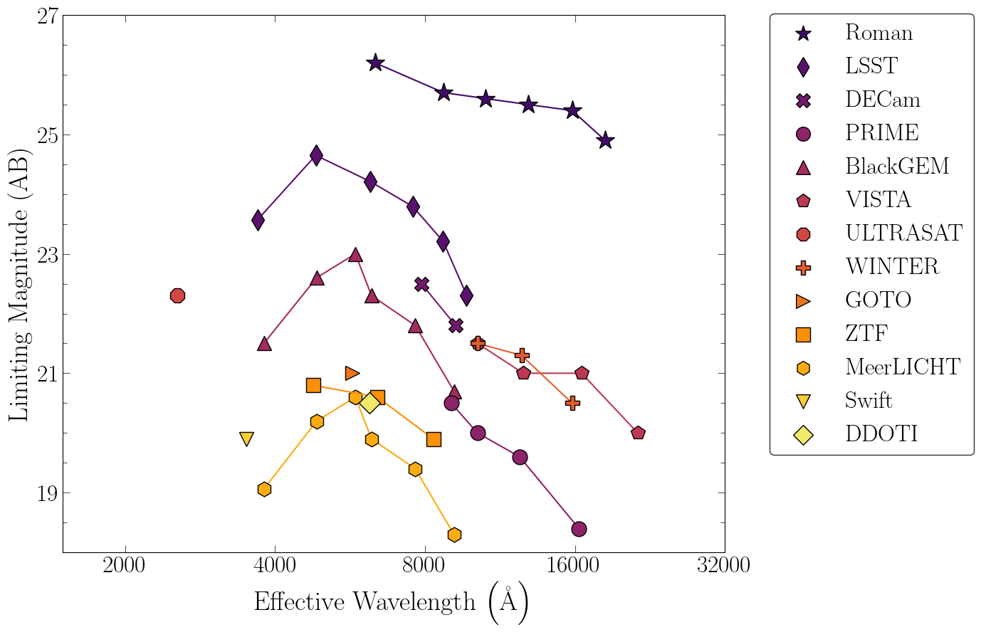
Figure 1: Limiting magnitudes for a selection of wide-field instruments. Each symbol corresponds to one instrument, with an instrument’s filters represented by its bandpass filter function’s effective wavelength. Lines connect filters from the same instrument. All limiting magnitudes are presented at the 5$\sigma$ confidence level, unless otherwise indicated in Table LABEL:tbl:kn.

BlackGEM $-$ BlackGEM is a planned array of wide-field optical telescopes located at the La Silla Observatory in Chile. It will initially consist of three 0.65-m optical telescopes, each with a 2.7 deg² FoV (Bloemen et al., 2015; Groot, 2019). Each telescope is equipped with a six-slot ($ugriz$ and broad $q$) filter wheel. The main focus of the BlackGEM mission is the follow-up of LIGO/Virgo/KAGRA candidate events, with a goal of achieving a cadence of two hours on low-latency sky localization using the $u$, $q$, and $i$ filters. In order to determine the most sensitive filters for KN detection, we also include $g$, $r$, and $z$ in our study. The $5\sigma$ limiting magnitude for a 300 s integration time under photometric observing conditions ($1\arcsec$ seeing) is $q\gtrsim 23$ mag (Paul Groot, 2021, Private Communication).

DDOTI $-$ DDOTI is a wide-field, robotic imager located at the Observatorio Astronómico Nacional (OAN) in Sierra San Pedro Mártir, Mexico (Watson et al., 2016). The instrument is comprised of six 28-cm telescopes with a combined 69 deg² FoV. DDOTI produces unfiltered images, referred to as the $w$-band. It has previously been using in the follow-up of GW190814 (Thakur et al., 2020). Based on DDOTI follow-up during O3 (Becerra et al., in prep.), we adopt a median exposure time of $\sim$ $2$ hr, yielding a median $10\sigma$ limiting magnitude $w\gtrsim 20.5$ mag.

DECam $-$ DECam is mounted on the 4-m Victor M. Blanco telescope at the Cerro Tololo Inter-American Observatory (CTIO) in Chile. The instrument has a 2.2 deg² FoV, and was designed for the purpose of wide-field optical ($ugrizY$) surveys (Flaugher et al., 2015). Electromagnetic follow-up of LIGO/Virgo candidate events has been carried out in previous observing runs by the Dark Energy Survey GW (DESGW) Collaboration (e.g., Soares-Santos et al., 2016, 2017; Andreoni et al., 2020; Herner et al., 2020; Morgan et al., 2020) using the $i$- and $z$-bands. In this work, we focus on kilonova detection by DECam at these wavelengths.

GOTO $-$ At design specifications, GOTO will include an array of $16\times$ 40-cm telescopes on two robotic mounts (producing a 160 deg² FoV) at two separate locations in Spain and Australia, allowing for coverage of both hemispheres (Dyer et al., 2018, 2020; Dyer, 2020). A prototype, referred to as GOTO-4 (18 deg² FoV), was instituted in La Palma, Spain in 2017 with an initial array of 4 telescopes. This was upgraded to an 8 telescope array in 2020 (GOTO-8), yielding a 40 deg² FoV (Dyer et al., 2020). The prototype mission, GOTO-4 has demonstrated its capability to cover large GW localization regions during O3 with good sensitivity to optical transients (Gompertz et al., 2020). In a 360 s integration time, GOTO can reach depths of $L\gtrsim 21.0$ mag (Ben Gompertz & Martin Dyer, 2021, Private Communication), where $L$ is a wide-band filter, approximately equivalent to $g+r$.

LSST $-$ The Vera C. Rubin Observatory, currently under construction on Cerro Pachon in Chile, has a planned first light in 2023. The observatory consists of an 8.4-m wide-field, optical telescope covering a 9.6 deg² FoV. The Rubin Observatory’s LSST will survey half the sky every three nights in the $ugrizy$ filters. The planned Wide-Fast-Deep (WFD) survey will reach $r\gtrsim 24.2$ mag (assuming airmass $\sim$ $1.2$) for a 30 s integration time (Ivezić et al., 2019). Despite the lack of a formal GW follow-up strategy, we have included LSST within this study to highlight the sensitivity of the WFD survey (see also, e.g., Scolnic et al., 2018; Cowperthwaite et al., 2019) in order to encourage GW follow-up, and demonstrate the prospect of serendipitous detection.

MeerLICHT $-$ MeerLICHT is a fully robotic 0.65-m optical telescope located at the South African Astronomical Observatory (SAAO) in Sutherland, South Africa (Bloemen et al., 2015). MeerLICHT was designed as the prototype instrument for the BlackGEM array (Groot, 2019). The telescope has a 2.7 deg² FoV, and covers the same $ugr(q)iz$ wavelengths as BlackGEM. MeerLICHT has been used for GW follow-up during past LIGO/Virgo observing runs (e.g., GW190814; de Wet et al., 2021) with observations in the $u$, $q$, and $i$ filters. For comparison to BlackGEM, we likewise include the $g$, $r$, and $z$ filters in our study. MeerLICHT is sky background limited in 60 s exposures, yielding a limiting magnitude $q\gtrsim 20.6$ mag.

PRIME $-$ PRIME is a 1.8-m wide-field infrared telescope under construction at SAAO. The telescope has a 1.56 deg² FoV, and covers wavelengths $ZYJH$. In a 100 s integration time PRIME reaches depths of $z\gtrsim 20.5$ mag and $Y\gtrsim 20.0$ mag (Takahiro Sumi, 2021, Private Communication).

Roman $-$ The 2.4-m Roman Space Telescope (formerly WFIRST), with planned launch in 2025, will cover a 0.28 deg² FoV ($\sim$ $200$ times larger than HST; Spergel et al., 2015). The Wide Field Instrument (WFI) is sensitive to optical/infrared wavelengths between 5000–20000 $\mathrm{\AA}$. In this study, we focus on the $RZYJHF$ filters. We have chosen to include Roman within this study in order to encourage GW follow-up (see also Foley et al., 2019), and demonstrate its sensitivity to kilonovae out to cosmological distances. The instrument sensitivity is adopted following Hounsell et al. (2018) and Scolnic et al. (2018).

UVOT $-$ The UVOT onboard the Neil Gehrels Swift Observatory has a wavelength coverage of 1600–8000 $\mathrm{\AA}$, and a 0.08 deg² FoV (Roming et al., 2005). Despite its smaller FoV, Swift is able to cover large regions of the sky in $<24$ hr with a rapid response (a few hours) to LIGO/Virgo alerts (Evans et al., 2016, 2017; Klingler et al., 2019; Page et al., 2020; Klingler et al., 2021). In addition, Swift has the added benefit of simultaneous X-ray coverage from the X-ray Telescope (XRT). UVOT follow-up has been optimized for its smaller FoV by targeting galaxies with high probabilities of being the host, ensuring they are completely within the FoV (Klingler et al., 2019). The large majority of UVOT tiles are observed with the $u$-band, and, therefore, we focus our analysis on this filter. Based on GW follow-up during O3, we adopt a median $5\sigma$ limiting magnitude $u\gtrsim 19.9$ mag (Oates et al., in prep.).

ULTRASAT $-$ ULTRASAT is an ultraviolet telescope with planned launch to geostationary orbit in 2024. The instrument will have a 200 deg² FoV, and cover wavelengths between 2200–2800 $\mathrm{\AA}$, referred to as $NUV$. The estimated limiting magnitude in 900 s integration time is $NUV\gtrsim 22.3$ mag. Since ULTRASAT does not have a publicly available filter function, we approximated the filter response with a top-hat function between 2200 and 2800 $\mathrm{\AA}$.

VISTA $-$ VISTA is a 4-m wide-field survey telescope equipped with the VISTA InfraRed CAMera (VIRCAM) covering wavelengths $ZYJHK_{s}$ with a $1.6$ deg² FoV (Sutherland et al., 2015). VISTA is located at the Cerro Paranal Observatory in Chile, and operated by the European Southern Observatory (ESO). Follow-up of LIGO/Virgo candidate events has largely occurred through the Vista Near infra-Red Observations Uncovering Gravitational wave Events (VINROUGE) project in the $Y$, $J$, and $K_{s}$ filters (e.g, Tanvir et al., 2017; Ackley et al., 2020). The $5\sigma$ limiting magnitudes were taken from the Vista Hemisphere Survey (McMahon et al., 2013; Banerji et al., 2015) and re-scaled to a 360 s exposure time, yielding $Y\gtrsim 21.5$ mag, $J\gtrsim 21.0$ mag, $H\gtrsim 21.0$ mag, and $K_{s}\gtrsim 20.0$ mag.

WINTER $-$ WINTER is a new infrared instrument, with planned first light in mid-2021 (Lourie et al., 2020; Frostig et al., 2020). WINTER will use a 1-m robotic telescope located at the Palomar Observatory in California, United States. The instrument has a $\sim$ 1 deg² FoV, and covers infrared wavelengths $YJH_{s}$. In a 360 s integration time, WINTER reaches $5\sigma$ depth $Y\gtrsim 21.5$ mag, $J\gtrsim 21.3$ mag, and $H_{s}\gtrsim 20.5$ mag (Nathan Lourie & Danielle Frostig, 2021, Private Communication).

ZTF $-$ ZTF employs a wide-field camera (47 deg² FoV) on the Palomar 48-in (P48) Oschin (Schmidt) telescope in San Diego County, California, United States (Bellm et al., 2019). Using 30 s exposures, it can cover 3760 deg² hr^-1 to limiting magnitude $r\gtrsim 20.6$ mag (Graham et al., 2019). This capability makes ZTF an effective tool for kilonova searches, both for GW candidate events (Coughlin et al., 2019; Kasliwal et al., 2020) and serendipitous discovery (Andreoni et al., 2021).

We note that the follow-up strategy and sensitivity of these instruments varies greatly depending on a number of factors, such as the observing conditions, sky location, and the size of the GW localization region. The sensitivity assumed in this work is considered to be an approximate limiting magnitude for GW follow-up, while noting that this sensitivity is variable day-to-day for each ground-based instrument. We also note that the limiting magnitudes are computed for “snapshot” exposures, and more sensitive images can be obtained by stacking multiple exposures over the course of a night. Figure 1 displays the assumed limiting magnitudes, indicating separate filters by their effective wavelength. For consistency, we compute effective wavelengths from all filter response functions using Eq. 1 of King (1952). These instruments provide an excellent coverage of the range of wavelengths expected for kilonovae. In Table LABEL:tbl:kn, we present the FoV, typical exposure time of GW tiling, filter effective wavelengths, and limiting magnitudes for each instrument.

3 Assessing Kilonova Detectability

Dyn. ejecta mass	$\{0.001,0.003,0.01,0.03,0.1\}$ $M_{\sun}$
Wind ejecta mass	$\{0.001,0.003,0.01,0.03,0.1\}$ $M_{\sun}$
Dyn. ejecta velocity	$\{0.05,0.15,0.3\}$ $c$
Wind ejecta velocity	$\{0.05,0.15,0.3\}$ $c$
Dyn. ejecta morphology	Toroidal (T; Cassini oval family; Korobkin et al. 2021)
Wind ejecta morphology	Spherical (S) or “Peanut” (P; Cassini oval family; Korobkin et al. 2021)
Dyn. ejecta composition	initial $Y_{e}=0.04$ (see Table 2 in Wollaeger et al. 2021)
Wind ejecta composition	initial $Y_{e}=0.27$ or $0.37$ (see Table 2 in Wollaeger et al. 2021)

We employ the Los Alamos National Laboratory (LANL) grid of kilonova simulations (Wollaeger et al., 2021) to assess each instrument’s ability to observe a kilonova. Rather than limiting our study to AT 2017gfo-like kilonovae, these radiative transfer simulations span a wide range of ejecta parameters, including expected values from both BNS and NSBH progenitors. The LANL simulations are two-component, multi-dimensional, axisymmetric kilonova models, generated with the Monte Carlo radiative transfer code SuperNu (Wollaeger et al., 2013; Wollaeger & van Rossum, 2014). These simulations rely on nucleosynthesis results from the WinNet code (Winteler et al., 2012; Korobkin et al., 2012) in addition to a set of tabulated binned opacities (Fontes et al., 2020) from the LANL suite of atomic physics codes (Fontes et al., 2015). The most recent LANL grid of kilonova simulations (Wollaeger et al., 2021) includes a full set of lanthanides and fourth row elements, some of which were not included in previous datasets (Wollaeger et al., 2018).

These radiative transfer simulations simultaneously evolve two ejecta components: a dynamical ejecta and wind ejecta component. The dynamical ejecta component is initiated with a low electron fraction ($Y_{e}=0.04$), and corresponds to the lanthanide-rich or “red” emission. This component has composition consistent with the robust “strong” r-process pattern such as the one repeatedly found in metal-poor r-process enriched stars and in the Solar r-process residuals (Sneden et al., 2009; Holmbeck et al., 2020). The second, lanthanide-poor wind ejecta component corresponds to the “blue” kilonova emission and is primarily composed of wind-driven ejecta from the post-merger accretion disk. The wind ejecta is initiated with two separate wind compositions, representing either high- ($Y_{e}=0.37$) or mid- ($Y_{e}=0.27$) latitude wind composition, consistent with winds induced by a wide range of post-merger remnants (Lippuner et al., 2017; Wollaeger et al., 2021). Dynamical ejecta is initiated with a toroidal morphology, constrained near the binary’s orbital plane, while the wind ejecta is modeled by either a spherical or “peanut-shaped” geometry (Korobkin et al., 2021). Figure 2 presents the two morphological configurations used in the simulation set. Models span five ejecta masses (0.001, 0.003, 0.01, 0.03, and 0.1$M_{\sun}$) and three ejecta velocities (0.05, 0.15, and 0.3$c$) for each component, covering the full range of kilonova properties anticipated from numerical simulations (see Wollaeger et al. 2021 and references therein). By considering all possible combinations of ejecta properties, the LANL grid includes 900 kilonova simulations. The full set of simulation parameters are compiled in Table LABEL:tbl:nome.

Figure 2: Schematics of the two combined morphologies used in the simulation grid (Wollaeger et al., 2021). All models have a toroidal (T, red) dynamical ejecta, 450 models are simulated with a spherical wind (S, blue), and 450 models are simulated with a peanut-shaped wind (P, blue). Each component is varied over the mass-velocity grid in Table LABEL:tbl:nome, and hence is not necessarily drawn to scale here (adapted from Korobkin et al. 2021 and Wollaeger et al. 2021).

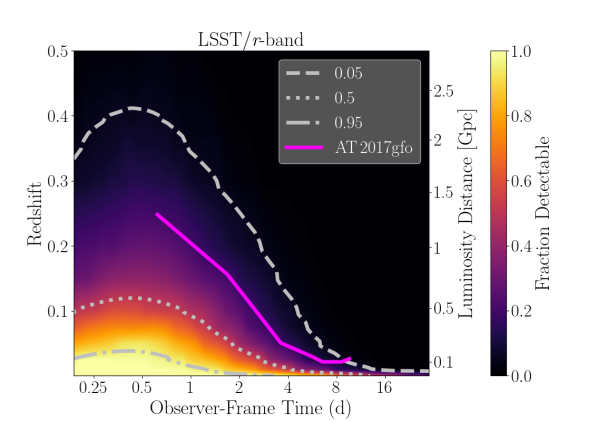
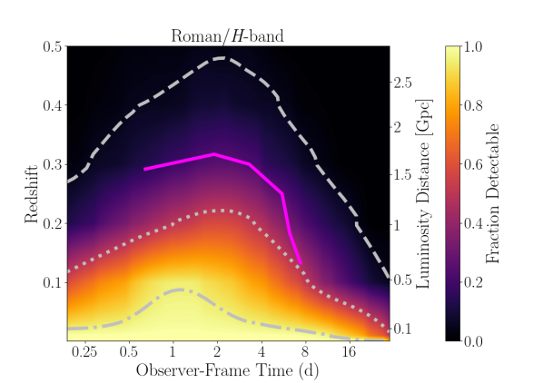
Figure 3: Detectability constraints for two filters: LSST/r-band (top) and Roman/H-band (bottom). Contours indicate the fraction of 48,600 simulated kilonovae (900 simulations each rendered at 54 viewing angles) with apparent magnitudes brighter than the limiting magnitude in each filter, for a given redshift and observer-frame time. The three white contours demarcate regions where 5%, 50%, and 95% of simulated kilonovae are detectable. The magenta curve represents each filter’s ability to detect AT 2017gfo-like kilonovae.

These 900 simulations have previously been used to estimate kilonova properties associated with follow-up of GW190814 (Thakur et al., 2020) and targeted observations of two cosmological sGRBs (O’Connor et al., 2021; Bruni et al., 2021). Additionally, the LANL simulation grid is the basis for an active learning-based approach to a kilonova lightcurve surrogate modeling and parameter estimation framework (Ristic et al., 2021).

All 900 multi-dimensional simulation are rendered in 54 viewing angles, each subtending an equal solid angle of $4\pi/54$ sr. In this study, we use spectra from all 54 viewing angle renditions to quantify detectability, making the generous assumption that a GW event has equal probability of detection with all viewing angles. This differs from kilonova searches aimed at sGRBs, such as in O’Connor et al. 2021, where we limit our simulation grid to face-on viewing angles ($\theta_{v}\lesssim 15.64^{\circ}$) as sGRBs are typically detected on-axis. By including all 54 viewing angles of the 900 LANL kilonova simulations, our detectability study incorporates a full suite of 48,600 kilonova models.

Each model includes a set of time-dependent spectra, which are converted to lightcurves by computing a magnitude associated with each spectrum. Spectra are not simulated for the first three hours post-merger (rest frame). We render each simulated spectra set into a lightcurve for various redshifts, $z$, and for a broad range of filters with corresponding wavelength-dependent bandpass filter functions $R\left(\lambda_{0}\right)$. Magnitudes are computed according to

$$m_{\mathrm{AB}}=-2.41-\frac{\int_{0}^{\infty}f\left(\lambda_{0}\left(1+z\right)^{-1}\right)R\left(\lambda_{0}\right)\lambda_{0}d\lambda_{0}}{\left(1+z\right)\int_{0}^{\infty}R\left(\lambda_{0}\right)\lambda_{0}^{-1}d\lambda_{0}},$$ (1)

where $\lambda_{0}$ is the observed wavelength and $f\left(\lambda_{0}\right)$ is the wavelength-dependent spectral flux density (Hogg et al., 2002; Blanton et al., 2003). In Equation 1, we account for cosmological K-corrections (Humason et al., 1956; Oke & Sandage, 1968) by converting rest-frame spectral emission to observer-frame wavelengths.

We define a kilonova as detectable in a given filter if it outshines the limiting magnitude of the filter, as listed in Table LABEL:tbl:kn. Then, we trace the detectability’s variation with redshift, by considering lightcurves at various cosmological distances. Figure 3 displays detectability constraints for two representative filters: the LSST r-band (optical) and the Roman Space Telescope’s H-band (near-infrared). We present detectability, defined as the fraction of detectable kilonova simulations, as a function of both redshift and observer-frame time. Detectability in the LSST/r-band decreases over time, as kilonovae optical emission fades within $\sim$1 day post-merger. However, the higher wavelength Roman/H-band reaches peak detectability two days post-merger, with 5% of nearby ($<$ 1 Gpc) kilonovae detectable over two weeks after merger. For comparison, Figure 3 includes detectability constraints for AT 2017gfo-like kilonovae, computed from spectroscopic data (Chornock et al., 2017; Cowperthwaite et al., 2017; Nicholl et al., 2017; Pian et al., 2017; Shappee et al., 2017; Smartt et al., 2017). We do not present AT 2017gfo-like detectability within 12 hours of merger, as no spectra were collected at this point in the kilonova evolution. Our AT 2017gfo-like detectability metrics are broadly consistent with previous studies (Scolnic et al., 2018; Rastinejad et al., 2021). Similar figures for all filters in Table LABEL:tbl:kn are available in Appendix A.

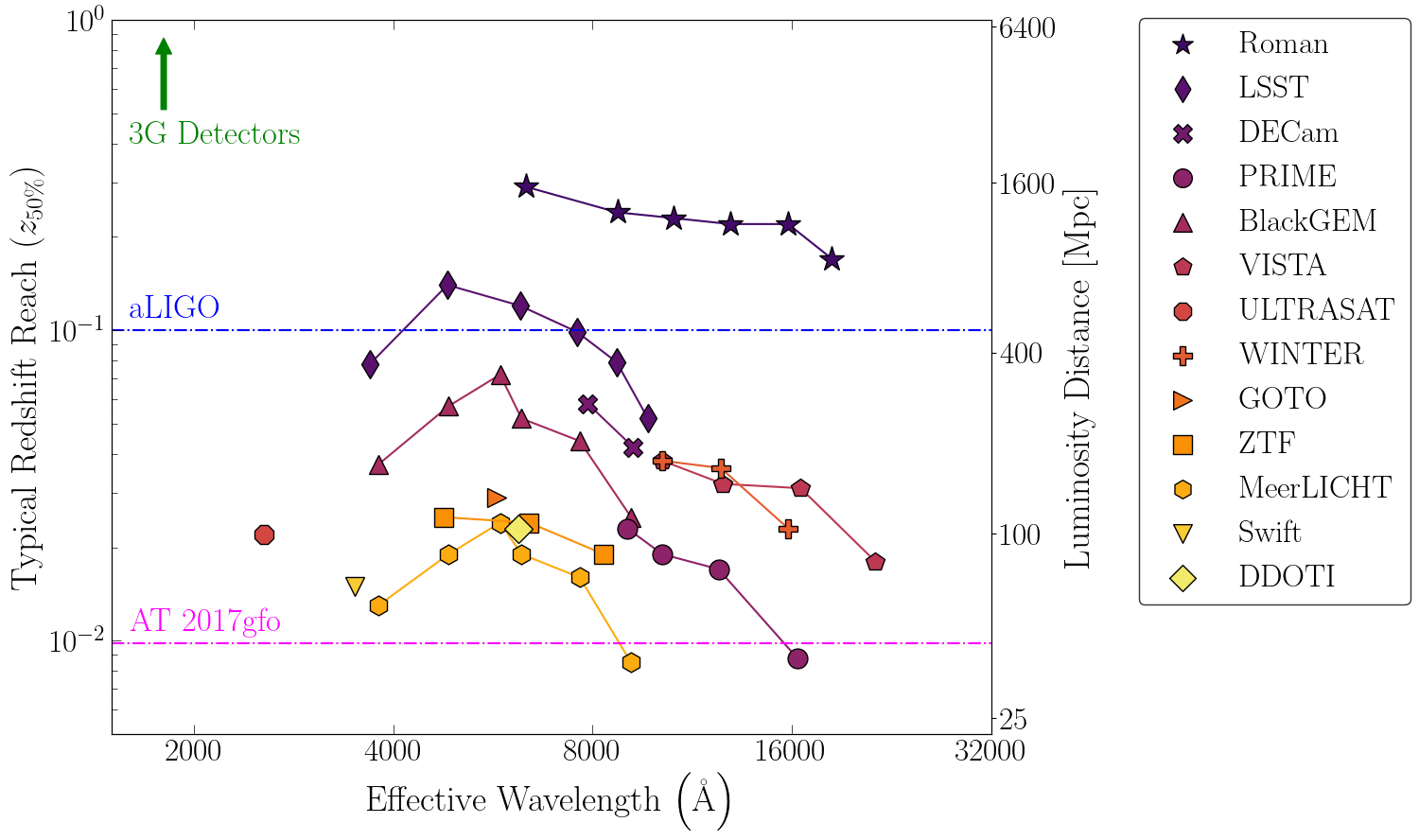
Figure 4: Typical redshift reach for a selection of instruments. The vertical axis indicates the maximum redshift at which 50% of the LANL simulated lightcurves are detectable in a given filter at any one time. Similarly to Figure 4, each symbol corresponds to one instrument, with an instrument’s filter represented by their bandpass filter function’s effective wavelength. Lines connect filters from the same instrument. The magenta horizontal line indicates the redshift of AT 2017gfo’s host galaxy (Kourkchi & Tully, 2017), while the blue line indicates the redshift horizon for a 1.4$M_{\sun}$ + 1.4$M_{\sun}$ BNS at advanced LIGO’s design sensitivity (Hall & Evans, 2019). Horizon redshifts for third-generation GW detectors, including Cosmic Explorer and Einstein Telescope, exceed the maximum redshift in the figure.

For each filter, we compute the maximum redshift at which 50% of simulated kilonovae are detectable at any one time, $z_{50\%}$, called the “typical redshift reach.” With this definition, we ascribe a typical redshift reach of $z_{50\%}=0.12$ and $z_{50\%}=0.22$ to the LSST/r-band and Roman/H-band in Figure 3, respectively. Table LABEL:tbl:kn lists the typical redshift reaches for all instruments and filters, in addition to compiling maximum detectable redshifts for both 95% and 5% of simulated kilonovae as $z_{95\%}$ and $z_{5\%}$, respectively.

Additionally, Figure 4 compares the typical redshift reach for all instruments in this study, highlighting the differences as a function of their effective wavelengths (see Table LABEL:tbl:kn). Typical redshift reaches vary from $z_{50\%}=0.0085$ ($\sim$38 Mpc) for the MeerLICHT/z-band up to $z_{50\%}=0.29$ ($\sim$1.5 Gpc) for the Roman/R-band. As anticipated, the typical redshift reach for each instrument correlates significantly with the limiting magnitude distribution in Figure 1. We remind the reader that simulated lightcurves are not available earlier than three hours post-merger (rest frame), resulting in no detectability predictions in this time range. This omission may bias the detectability estimates of low-wavelength (ultraviolet) filters, such as the ULTRASAT/$NUV$-band, LSST/u-band, and UVOT/u-band.

4 Detectability Variations with Kilonova Properties

The typical redshift reach often varies significantly with kilonova properties, such as the ejecta mass or velocity. Larger ejecta masses generally result in more luminous kilonova emission, allowing for detection at higher redshifts, while kilonovae containing lower ejecta masses are only detectable at nearby distances. This mass dependency makes it difficult to determine whether a GW candidate event will produce an observable kilonova for a given instrument. Robust detectability metrics are further muddled by compounding degeneracies with other parameters such as velocity of the expanding ejecta, viewing angle, and composition.

Differing kilonova properties induce variations in kilonova detectability. For example, a kilonova with large wind ejecta mass and small dynamical ejecta mass may be easily detectable in the ultraviolet but difficult to observe in near-infrared filters, while other kilonova parameters may produce emission that is primarily detectable in the infrared. Lower-wavelength filters probe the wind ejecta, with peak emission in optical wavelengths at early times. At the low-wavelength extreme, ultraviolet instruments capture the early structure of the outermost wind-driven ejecta (Arcavi, 2018; Banerjee et al., 2020). However, these low-wavelength filters offer little insight into the dynamical ejecta, which peaks at redder wavelengths. Additionally, a filter’s variation with kilonova parameters depends on the source redshift: high-redshift kilonova emission is shifted to higher wavelengths, requiring subsequently redder filters to capture variability in dynamical ejecta mass. If kilonovae properties are unknown, multi-band observations across UVOIR wavelengths are necessary to maximize the probability of kilonova detection.

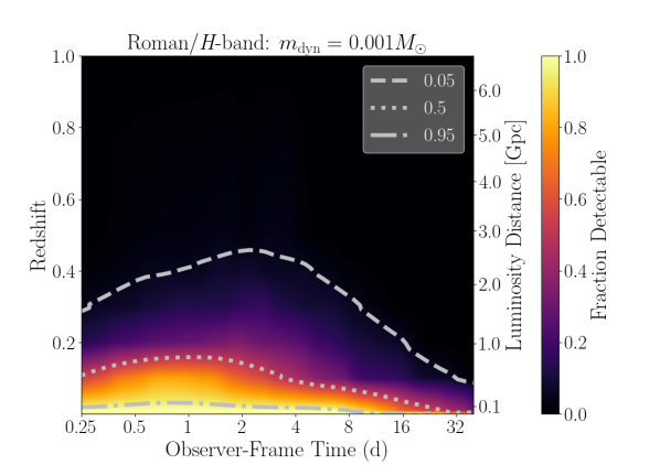
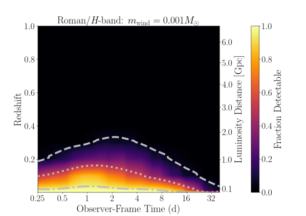
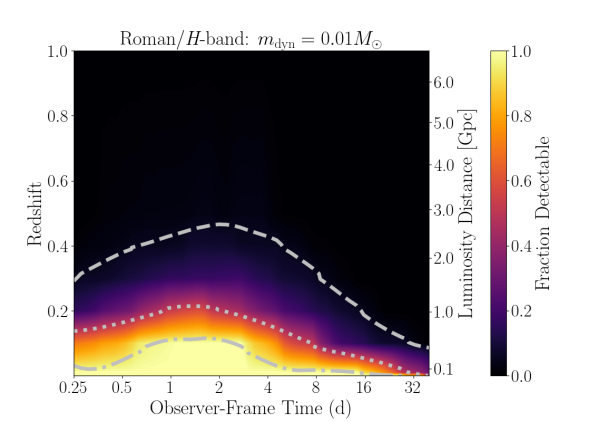
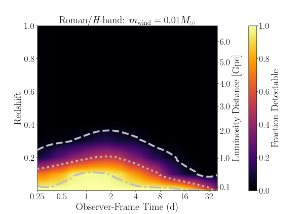
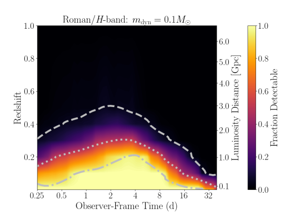
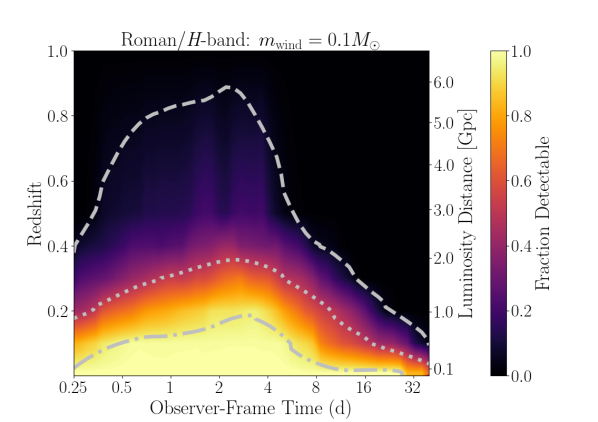
Figure 5: Detectability constraints for the Roman/H-band for six sets of kilonova simulations. The left column represents variation with dynamical ejecta mass, while the right presents variation with wind ejecta mass. The top row corresponds to lower masses (0.001$M_{\sun}$), middle row corresponds to an intermediate mass (0.01$M_{\sun}$), while the bottom row present high ejecta masses (0.1$M_{\sun}$). We place no restrictions on ejecta velocities, morphology, composition, or viewing angle, such that each panel includes 9720 simulations (180 simulated kilonovae each with 54 viewing angles) of the full set of 48,600 LANL kilonovae.

Figure 5 demonstrates the variation in kilonova detectability in the Roman/H-band for different ejecta masses. The left (right) column restricts the simulation set to one dynamical (wind) ejecta mass, while allowing all other parameters to vary, resulting in 9720 simulations per panel (180 simulations each with 54 viewing angles). In the left column, dynamical ejecta mass varies from the lowest (0.001$M_{\sun}$) to the largest (0.1$M_{\sun}$) values in the LANL simulation grid. Larger ejecta masses enhance detectability, as 50% of simulations with dynamical ejecta masses of 0.1$M_{\sun}$ are detectable out to $z=0.31$, with peak emission three days post-merger. Lower ejecta masses induce both dimmer emission and an earlier peak timescale (e.g., Kasen et al., 2017), as shown by the diminished late-time detectability and smaller typical redshift reach ($z=0.16$) for dynamical ejecta masses of 0.001$M_{\sun}$. However, a small subset of kilonovae with low dynamical ejecta masses remain detectable at redshifts $z>0.3$, consistent with the addition of a large wind ejecta mass. The variation is a bit more pronounced for wind ejecta: 50% of simulated kilonovae with large wind ejecta masses (0.1$M_{\sun}$) are detectable out to $z=0.37$, while less than 5% of low wind ejecta (0.001$M_{\sun}$) kilonovae are detectable at such high redshifts. Additionally, as higher redshift ($z\gtrsim 0.4$) kilonova emission is proportionally shifted to higher wavelengths, the Roman/H-band becomes less effective at detecting emission from high dynamical ejecta mass mergers. As a result, variation with dynamical ejecta mass decreases with redshift.

Different wavelength bands exhibit varying dependency on ejecta mass. Similarly to in the near-infrared (Roman/H-band), detectability at optical and ultraviolet wavelengths varies significantly with wind ejecta masses. However, optical and ultraviolet bands show little variability with dynamical ejecta masses. We define the variable $v$ to quantify a given filter’s sensitivity to a kilonova property such as ejecta mass. As an example, we can quantify the Roman/H-band’s dependence on wind ejecta mass by comparing the 50% detectability contours (dot–dashed lines) in Figure 5. We label the 50% detectability contour for the lowest ejecta mass (top panel) and highest ejecta mass (bottom panel) as $g(t)$ and $f(t)$, respectively. We then quantify variability with mass as:

$$v=\frac{\int_{t_{\mathrm{min}}}^{t_{\mathrm{max}}}\left|f\left(t\right)-g\left(t\right)\right|dt}{\frac{1}{2}\int_{t_{\mathrm{min}}}^{t_{\mathrm{max}}}\left[f\left(t\right)+g\left(t\right)\right]dt},$$ (2)

integrating from the smallest rest-frame time, $t_{\mathrm{min}}=0.125$ d, to a maximum time of $t_{\mathrm{max}}=20$ d. Values of $v$ close to zero indicate negligible variation with a given parameter, while higher values of $v$ indicate a significant dependence. There is no upper limit on $v$, although we note that a value of $v=1$ corresponds to a three-fold enhancement in $z_{50\%}$ between two subsets of parameters (i.e. $f\left(t\right)=3g\left(t\right)$). Based on the 50% contours in Figure 5, the Roman/H-band produces $v=0.91$ for dynamical ejecta mass (left column) and $v=0.94$ for wind ejecta mass (right column), suggesting that the Roman/H-band’s detectability is slightly more dependent on wind ejecta mass than dynamical ejecta mass.

Figure 6 presents the variability scores for all filters in Figure 4 as a function of both dynamical ejecta mass (purple) and wind ejecta mass (orange). As anticipated, variability with dynamical ejecta mass increases with filter wavelength, while wind ejecta mass variability decreases with wavelength. Ultraviolet filters exhibit the largest dependence on wind ejecta mass, with the UVOT/u-band and ULTRASAT/NUV-band both yielding $v=1.7$. The PRIME/$H$-band demonstrates the largest variability with dynamical ejecta mass, with $v=1.3$. Variability scores directly relate to a filter’s ability to constrain a given parameter from photometric observations (see Section 5).

The interplay between various kilonova parameters must be considered to fully capture variations in detectability. For example, masses for both dynamical and wind ejecta alter kilonova emission, and thus affect detectability. We explore the interrelation of dynamical and wind ejecta masses in Figure 7, using the Roman/H-band as an example. The top (bottom) panel restricts total ejecta mass to the lowest (highest) simulated mass, where total mass is the sum of both dynamical and wind ejecta masses. In both panels, the total mass is fixed while composition, morphology, viewing angles, and ejecta velocities vary, resulting in 1944 simulations in each panel (36 simulations each rendered at 54 viewing angles). Total mass significantly alters kilonova detectability in the Roman/H-band, with a variability $v=1.6$ between the total masses of 0.002$M_{\sun}$ (top panel) and 0.2$M_{\sun}$ (bottom panel). Kilonovae with higher total ejecta masses are detectable at significantly higher redshifts than their low mass counterparts.

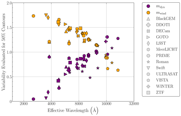
Figure 6: Mass-dependent variability for a selection of filters. Each symbol corresponds to one instrument, with an instrument’s filters represented by their bandpass filter function’s effective wavelength. The vertical axis represents each filter’s dependence to either dynamical ejecta mass (purple) or wind ejecta mass (orange), as defined in Equation 2. Higher-wavelength filters are increasingly sensitive to variations in dymamical ejecta mass, while dependence on wind ejecta mass decreases with increasing filter wavelength.

In addition to mass, other properties of neutron star mergers affect kilonova detectability. Luminosity may vary with viewing angle due to morphological effects (Korobkin et al., 2021) and lanthanide curtaining (Kasen et al., 2015). Additionally, ejecta composition significantly alters detectability in some filters, as lanthanide-poor ejecta yields significantly less luminous emission in the redder optical and infrared filters than mergers with lanthanide-rich ejecta. Ejecta velocity also has a pronounced effect on detectability, with higher ejecta velocities leading to earlier peak emission and subsequently more luminous kilonovae (e.g., Kasen et al., 2017). Numerous other factors alter simulated lightcurves and kilonova detectability including decay product thermalization and nuclear mass models (Lippuner & Roberts, 2015; Hotokezaka & Nakar, 2020). Considerably more uncertain nuclear physics may be propagated by allowing synthesized r-process abundance patterns to differ from the robust “strong” pattern, as done in Barnes et al. (2020) and Zhu et al. (2021).

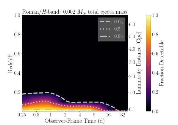
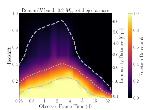
Figure 7: Detectability constraints for the Roman/H-band for two total ejecta masses, corresponding to the sum of dynamical and wind ejecta masses. The top panel displays the smallest total ejecta mass (0.002$M_{\sun}$), while the bottom panel corresponds to the largest total ejecta mass (0.2$M_{\sun}$). We place no restrictions on morphology, composition, viewing angle, or ejecta velocity, such that each panel includes 1944 simulations (36 simulations each with 54 viewing angles) of the full set of 48,600 LANL kilonova simulations.

5 Inferring Kilonova Properties with Wide-Field Observations

We can leverage parameter-dependent variations in kilonova detectability to infer ejecta properties and guide future observations. By coupling non-detections in wide-field transient searches with the kilonova detectability metrics presented in this work, constraints can be placed on kilonova ejecta properties. Non-detections are particularly constraining when a very large fraction of the GW sky localization is covered by multiple instruments or filters in a short period of time. To explore this, we consider observations in the Roman/H-band taking place two days post-trigger for a merger with a predicted redshift of $z=0.2$ (an ambitious $\sim$1 Gpc for current GW detectors). If these observations yield no transient detection, the total ejecta mass of an associated kilonova can be constrained to lower masses. This relationship is supported by Figure 7, as nearly 100% of simulated kilonovae with total ejecta masses of 0.2$M_{\sun}$ are detectable two days post-merger at $z=0.2$, while no kilonovae with total ejecta masses of 0.002$M_{\sun}$ are detectable. Thus, a non-detection rules out the presence of a high-ejecta mass kilonova at $z=0.2$.

This method has previously been employed by Thakur et al. 2020 to constrain parameters for a plausible kilonova associated with GW190814 (Abbott et al., 2020d). The authors compare upper limits from wide-field searches (including DDOTI) to the LANL kilonova grid, ruling out the presence of a high-mass ($>$ 0.1$M_{\sun}$) and fast-moving (mean velocity $\geq 0.3c$) wind ejecta. Total ejecta masses $\geq$ 0.2$M_{\sun}$ are also strongly disfavored by the upper limits.

Non-detections in wide-field searches may also guide subsequent observing schedules. For example, assume that you are planning additional follow-up observations after a non-detection in the BlackGEM/q-band at 12 hours post-merger for an event at $z=0.05$ ($\sim$230 Mpc) that has not been detected by any other instrument. Of all the instruments in this study intended to follow-up GW candidate events (i.e. not including LSST or Roman), an additional BlackGEM observation is best suited for follow-up observations. This conclusion was reached by searching the 48,600 LANL kilonova models to identify kilonovae that are undetectable with BlackGEM at this redshift and time, but detectable with other instruments between 12 and 36 hours post-merger. Based on the LANL kilonova grid, 8% of simulated kilonovae are detectable 36 hours post-merger in the BlackGEM/q-band, but not detectable 12 hours post-merger. A selection of detectable lightcurves is highlighted in the left panel of Figure 8, suggesting the presence of high mass ($\geq$ 0.03$M_{\sun}$) and slow-moving (mean velocity $<0.15c$) wind ejecta. BlackGEM’s q-band does not offer strong constraints on dynamical ejecta properties, consistent with the discussion in Section 4 and Figure 6. DECam can also provide useful follow-up observations after a non-detection at 12 hours, with 6% of simulated kilonovae detectable in DECam but not BlackGEM at the aforementioned times. Several instruments, including DDOTI, GOTO, VISTA, and PRIME, have negligible probability of detecting a kilonova at $z=0.05$ following a BlackGEM non-detection. However, we note that both LSST and Roman have the highest probability of detecting a kilonova in this scenario, further highlighting their utility in kilonova searches.

We performed a similar analysis assuming a non-detection with WINTER (J-band) 12 hours post-merger for a GW event at $z=0.05$ ($\sim$230 Mpc). Again, we searched the 48,600 LANL kilonova models for kilonovae that are undetectable with the WINTER/J-band at this redshift and time, but detectable with other instruments between 12 and 36 hours post-merger. Based on the LANL kilonova grid, 16% of simulated kilonovae are detectable with the WINTER/J-band 36 hours post-merger but not detectable 12 hours post-merger. These lightcurves are highlighted in the right panel of Figure 8. The WINTER non-detection and subsequent detection are consistent with large ejecta masses, with over 70% of orange lightcurves in Figure 8 corresponding to total ejecta masses $\geq$ 0.1$M_{\sun}$. WINTER’s J-band offers constraints on both dynamical and wind ejecta parameters, as expected from Figure 6. In addition to WINTER, several instruments in this study are capable of observing kilonovae following a WINTER non-detection. For example, over 40% of simulated lightcurves are observable in the BlackGEM/q-band at 36 hours post-merger following a WINTER non-detection 24 hours earlier. Additional instruments have non-zero probabilities of detecting a kilonova under this scenario: GOTO can observe 6% of simulated kilonovae following a WINTER non-detection, DDOTI can observe 12%, VISTA can observe 15%, ZTF can observe 3%, and ULTRASAT can observe 1%.

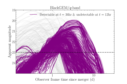
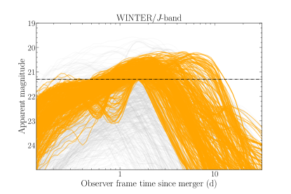
Figure 8: Simulated kilonova lightcurves, in the observer frame, in the BlackGem/q-band (left) and WINTER/J-band (right) for a merger at $z=0.05$ ($\sim$230 Mpc). Purple and orange lightcurves are detectable at 36 hours but undetectable at 12 hours in the selected filter. Gray lightcurves do not meet this criterion. Horizontal dot–dashed lines correspond to limiting magnitudes in each filter. Only a subset of the full LANL kilonova grid is displayed, for clarity. These panels also highlight the variation in lightcurve behavior between optical (BlackGEM) and near-infrared (WINTER) filters.

These examples demonstrate how non-detections offer powerful constrains on kilonova ejecta properties. However, targeted observations with large aperture telescopes are better suited to sample kilonova emission after an initial detection in a wide-field search, providing multi-band observations over the duration of kilonova evolution. The LANL set of kilonova models provides a rich data set for thorough statistical analysis and optimization of kilonova observing strategies, beyond the study of non-detections in wide-field surveys, which we reserve for future work. In addition, we refer the reader to several other studies on the efficacy of Bayesian parameter estimation to infer kilonova parameters (i.e. Coughlin et al., 2018; Barbieri et al., 2019; Nicholl et al., 2021; Heinzel et al., 2021; Ristic et al., 2021).

6 Instrument Results

In this section, we briefly summarize each instrument’s capacity for kilonova detection. We describe the accessible redshifts for each filter and the most probable times for kilonova detection. Additional figures for each instrument are presented in Appendix A.

BlackGEM $-$ BlackGEM’s optical and near-infrared filters are well-suited to detect kilonova emission, especially within two days post-merger. The broad q-band provides the best opportunities for detection, with 50% of simulated kilonovae detectable at $z=0.072$ ($\sim$340 Mpc) and high wind ejecta mass kilonovae detectable out to $z\sim 0.2$. Our results largely support BlackGEM’s plan to follow-up with the u, q, and i filters. However, we note that the z-band increases the detectable kilonova parameter space at later times ($t\geq 2$ d). As an example, nearly 10% of modeled kilonovae at $z=0.01$ ($\sim$45 Mpc) are only observable in the z-band at $t=4$ d (observer frame) and not observable in any other BlackGEM filters.

DDOTI $-$ DDOTI’s $w$ filter can detect 50% of simulated kilonovae out to $z=0.023$ ($\sim$100 Mpc), with a peak detectability 12 hours post-merger. DDOTI can follow-up some LIGO/Virgo/KAGRA candidate events with inferred redshifts out to $z=0.073$ ($\sim$340 Mpc).

DECam $-$ DECam’s i- and z-bands are sensitive to kilonova detection, reaching $z_{50\%}$ of 0.058 ($\sim$270 Mpc) and 0.042 ($\sim$190 Mpc), respectively. Despite its lesser sensitivity the z-band may be better suited to detect kilonovae than the i-band, as nearly all simulated kilonovae detectable in the i-band are also detectable by the z-band. DECam is able to observe high ejecta mass kilonovae out to $z=0.18$ ($\sim$900 Mpc).

GOTO $-$ GOTO’s L-band achieves a $z_{50\%}=0.029$ ($\sim$130 Mpc), with peak detectability $\sim$8 hr post-merger. GOTO is able to follow-up high wind ejecta mass LIGO/Virgo/KAGRA candidate events with inferred redshifts out to $z=0.097$ ($\sim$460 Mpc).

LSST $-$ LSST can observe the most distant kilonovae out of all other ground-based instruments in the study. The g-band reaches the highest typical redshift reach, with a $z_{50\%}=0.14$ peaking $\sim$8 hr post-merger. We especially encourage the use of LSST’s g, r, and i filters for follow-up of relatively distant LIGO/Virgo/KAGRA candidate events ($z=0.15-0.5$) that may not be observable with other ground-based, wide-field instruments.

MeerLICHT $-$ Similarly to BlackGEM, MeerLICHT’s broad q filter is the most sensitive at detecting kilonovae. MeerLICHT has better chances to observe kilonovae located at $z<0.074$ ($\sim$345 Mpc). For comparison, BlackGEM can detect kilonovae at over twice the distance of MeerLICHT.

PRIME $-$ This ground-based infrared instrument is useful for late-time kilonova searches, with peak detectability between one and eight days post-merger. The most sensitive filter reaches a $z_{50\%}=0.023$ ($\sim$100 Mpc), with some high ejecta mass kilonovae detectable out to $z=0.067$ ($\sim$300 Mpc). Additionally, the PRIME/H-band may offer strong constraints on dynamical ejecta masses.

Roman $-$ Roman provides an excellent tool for kilonova detection and GW follow-up. The Roman/R-band is the most sensitive filter in our study, reaching $z_{50\%}=0.29$ with some kilonovae detectable out to $z\sim 1$. However, Roman’s relatively small FoV precludes follow-up of GW candidate events with large localization areas. We encourage the use of the Roman Space Telescope for GW follow-up (see also Foley et al., 2019), especially for distant and/or well-localized candidate events.

UVOT $-$ Swift/UVOT’s u-band reaches a $z_{50\%}=0.015$ ($\sim$70 Mpc), with a peak detectability around four hours post-merger. The u-band is well-suited to follow-up LIGO/Virgo/KAGRA candidate out to $z=0.061$ ($\sim$280 Mpc). UVOT’s detectability estimates may be biased by the lack of simulated lightcurves within three hours post-merger.

ULTRASAT $-$ ULTRASAT provides an excellent tool for early kilonova detection. It’s 200 deg² NUV filter can detect 50% of simuilated kilonovae out to $z=0.022$ ($\sim$100 Mpc), with high wind ejecta mass mergers detectable out to $z=0.1$ within the first 12 hours post-merger. We caution the reader in their interpretation of ULTRASAT results. This study is based on an approximate ULTRASAT filter, as no finalized filter is publicly available. We anticipate that ULTRASAT’s detectability estimate would increase with the availability of simulated lightcurves before three hours.

VISTA $-$ VISTA is one of the most sensitive ground-based infrared facilities in the study, with $z_{50\%}=0.038$ ($\sim$170 Mpc) for the Y-band. VISTA is able to follow-up high ejecta mass LIGO/Virgo/KAGRA candidate events out to $z=0.094$ ($\sim$450 Mpc) one day post-merger. Additionally, VISTA observations may provide strong constraints on dynamical ejecta masses.

WINTER $-$ Similarly to VISTA, WINTER is one of the most sensitive ground-based infrared facilities in the study, with $z_{50\%}=0.038$ ($\sim$170 Mpc) for the Y-band. WINTER is capable of follow-up some nearby (within $\sim$ 100 Mpc) mergers over two weeks post-merger. WINTER can observe high ejecta mass kilonovae out to $z=0.093$ ($\sim$440 Mpc) one day post-merger, in addition to offering tight constraints on dynamical ejecta mass.

ZTF $-$ ZTF is well-suited to search large sky localization regions for relatively nearby kilonovae ($z\lesssim 0.1$), with a typical redshift reach of $z\sim 0.02$ ($\sim$100 Mpc) in the g-, r-, and i-bands. ZTF is able to detect a subset of high ejecta mass kilonovae out to $z=0.094$ ($\sim$445 Mpc).

7 Discussion & Conclusions

This study explores kilonova searches with current and upcoming wide-field instruments. This analysis relies on the LANL grid of kilonova simulations (Wollaeger et al., 2021), a set of 48,600 radiative transfer models which span a variety of ejecta parameters. Based on these simulations, we quantify each instrument’s ability to detect a kilonova, recording the fraction of observable kilonovae from the simulation grid for various times and redshifts. The 44 filters in this study have significant variations in their typical redshift reach; ultraviolet filters are restricted to observing nearby kilonovae ($z<0.3$), while the Roman Space Telescope can observe a subset of kilonovae out to $z\sim 1$. We concentrate on wide-field kilonova searches following a GW candidate event, although the conclusions of this study are equally relevant to kilonova searches following poorly-localized short GRBs. Additionally, the framework presented in this study is easily adaptable, and can be applied to searches performed by more sensitive, smaller FoV instruments (e.g., Gemini, Keck, GTC, VLT, SALT, HST, JWST) following the detection of a kilonova. Additionally, we remind the reader that the facilities studied in this work do not constitute a comprehensive selection of wide-field instruments.

Detecting, analyzing, and modeling kilonovae is a new and evolving science; many uncertainties remain after only a single confident multi-messenger observation with GWs (Abbott et al., 2017d). As a result, the models that lay the foundation of this study rely on numerous physical assumptions, including the use of a specific nuclear mass model (FRDM, Möller et al., 1995) and decay product thermalization (Barnes et al., 2016; Rosswog et al., 2017). While the LANL grid of kilonova models covers a wide range of kilonova parameters (see Section 3 and Table LABEL:tbl:nome), this simulation grid does not span all possible ejecta scenarios. For instance, the simulations do not encompass all possible variations in ejecta morphology (Korobkin et al., 2021) or composition (Even et al., 2020). We also ignore changes in the detected UVOIR emission due to extinction or the presence of contamination from either a sGRB afterglow or host galaxy, which will be expanded upon in a future work.

Our work produces results that are consistent with the detectability study presented by Scolnic et al. (2018), which determined kilonova detectability using an AT 2017gfo-like model. Scolnic et al. (2018) predict a redshift range of $z=0.02-0.25$ for LSST, consistent with our redshift range of $z=0.035-0.48$ for the most sensitive LSST filter. Our results are also broadly consistent with the detectability estimates presented by Rastinejad et al. (2021), which leveraged three kilonova models (in addition to AT 2017gfo) to infer the maximum redshift of kilonova detection.

Similarly to Scolnic et al. (2018), we focus only on the ability of these instruments to detect a kilonova, and not its unambiguous identification (as this outcome depends on multi-epoch observations across a range of filters). Wide-field searches are likely to uncover numerous other transient signals (e.g., supernovae), potentially masquerading as a kilonova signal (see Cowperthwaite & Berger 2015 for a discussion of kilonova contaminants). LIGO/Virgo/KAGRA candidate events constrained to large localization volumes are increasingly likely to reveal false positive kilonova candidates, further necessitating the need for repeated observations of each field to rapidly distinguish a kilonova candidate. In future work, we intend to provide methods to disentangle kilonova candidates from other transients with a limited number of photometric observations.

We caution the reader in the interpretation of our results and emphasize that the typical redshift reach values presented in Table LABEL:tbl:kn and Figure 4 refer to the redshifts at which 50% of simulated kilonovae are detectable. This is not equivalent to the probability of detection for the full population of kilonovae. For example, our results claim that 50% of simulated kilonovae are observable in the LSST/r-band at $z=0.12$. This does not imply that the LSST/r-band has a 50% probability of observing a kilonova at $z=0.12$. Such a statement relies on a realistic astrophysical distribution of kilonova ejecta properties, while our study is based on a uniformly sampled grid of models. This study could be expanded to draw from a distribution of kilonova models with the availability of more robust models for binary neutron star populations, neutron star equation of state, and mappings between compact object progenitors and ejecta. Additionally, this work could be further expanded to include redshift-dependent rates of neutron star mergers and associated GW detection.

Multi-band observations capture variability in kilonova emission and provide tighter constraints on kilonova properties, such as the composition and ejecta mass. Once a kilonova is identified, targeted follow-up observations at several wavelengths (and times) are necessary to constrain ejecta properties. Additionally, instruments must be distributed in geographically disparate locations, similarly to the Las Cumbres Observatory Global Telescope Network (Brown et al., 2013), to maximize the probability of kilonova detection. Instrument response time may also vary significantly based on the location of a neutron star merger on the sky. We stress the utility of both ground-based and space-based detectors to allow for rapid follow-up post-trigger, aiding in kilonova detection.

Kilonova searches also benefit from a variety of fields-of-view and exposure times, such as the collection of instruments in this study. Wide FoV instruments with short exposure times are best suited to rapidly scan the sky for GW candidate events localized to large regions of the sky, while smaller FoV instruments with longer exposure times are better suited for well-localized ($\lesssim$ 10 deg²) events. For example, while the Roman Space Telescope has the largest typical redshift reach in this study, less sensitive, wider FoV instruments are better able to follow-up GW candidate events with large localization areas.

Based on the results of our study, we present the following findings to guide observing strategies and commissioning of future instruments:

1. This study demonstrates the utility of a diversity of wide-field instruments to search for kilonovae following GW detections. This includes a variety in instrument location, sensitivity, FoV, cadence, exposure time, and wavelength coverage. Additionally, rapid dissemination of both GW and electromagnetic search results is critical to optimize counterpart searches among this diverse array of instruments.

2. Early observations increase the probability of observing a kilonova, especially at ultraviolet and optical wavelengths. Based on the results in this study, we stress the importance of early-time observations for kilonova detection. Although not a focus of this study, we note that early observations offer the most stringent constraints on wind ejecta properties.

3. More sensitive wide-field ultraviolet instruments are needed for kilonova detection as LIGO/Virgo/KAGRA reach design sensitivity. The ultraviolet instruments in this study can observe only a small fraction of kilonovae beyond $z\sim 0.1$, which is equivalent to the BNS horizon redshift of advanced LIGO at design sensitivity (Abbott et al., 2020b).

4. We promote the construction of additional wide-field near-infrared instruments. Compared to optical instruments, few ground-based near-infrared instruments are available for GW follow-up, potentially reducing the probability of kilonova detection. Near-infrared instruments hold immense promise for kilonova detection, as they are able to detect kilonovae within several days post-merger as opposed to the limited timescale accessible to ultraviolet and optical instruments.

5. We recommend using this work as a guide for scheduling future kilonova observations. Based on the results of this study, we encourage observations if more than 5% of simulated kilonovae are detectable at a given time and redshift based on the figures in Appendix A.

6. Low-latency GW products, such as sky localization and distance estimates, should be used to alter observing strategies. We recommend comparing low-latency distance estimates to the detectability estimates provided in this work.

The current and upcoming wide-field instruments in this study are well-poised to observe kilonovae coincident with GW events in the advanced detector era. However, the landscape of multi-messenger astronomy with GWs will change through the construction of new detectors. Sky localization will improve as additional GW detectors are commissioned (Abbott et al., 2020b), allowing larger aperture instruments to cover higher percentages of the localization region. Simultaneously, enhanced GW detector sensitivity will reveal neutron star mergers at cosmic distances previously inaccessible through GWs alone, with the Einstein Telescope and Cosmic Explorer detecting BNS mergers at redshifts of out to $z\sim 4$ and $z\sim 10$, respectively (Hall & Evans, 2019). To match the increase in GW detector sensitivity, innovative UVOIR instruments must be constructed to observe kilonovae in the era of third-generation GW detectors.

Appendix A Supplementary Figures

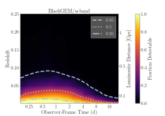
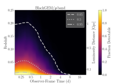
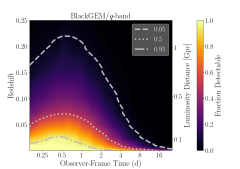
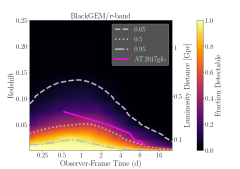
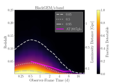
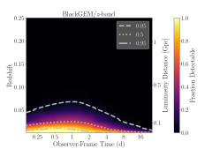
Figure 9: Detectability constraints for six BlackGEM filters. Contours indicate the fraction of 48,600 simulated kilonovae (900 simulations each rendered at 54 viewing angles) with apparent magnitudes brighter than the limiting magnitude in each filter, for a given redshift and observer-frame time. The three white contours demarcate regions where 5%, 50%, and 95% of simulated kilonovae are detectable. The magenta curve represents each filter’s ability to detect AT 2017gfo-like kilonovae; we only present AT 2017gfo-like detectability for filters that are fully spanned by AT 2017gfo spectral observations.

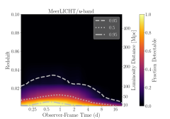
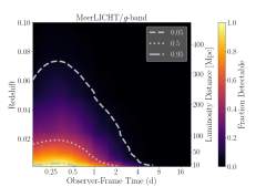
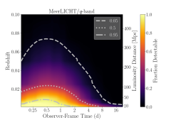
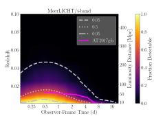
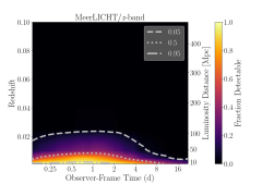
Figure 10: Detectability contours for MeerLICHT (see Figure 9 caption).

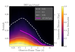
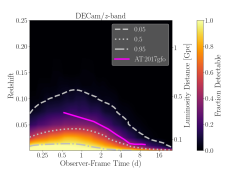
Figure 11: Detectability contours for DECam (see Figure 9 caption).

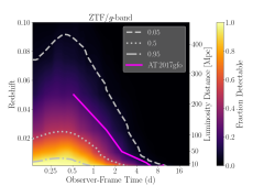
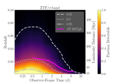
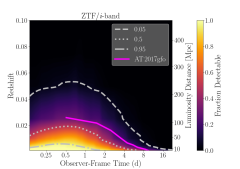
Figure 12: Detectability contours for ZTF (see Figure 9 caption).

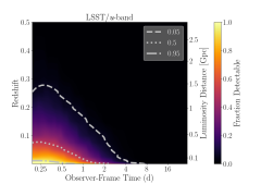
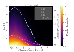
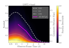
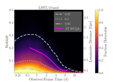
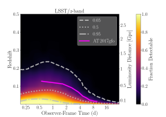
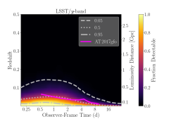
Figure 13: Detectability contours for LSST (see Figure 9 caption).

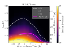
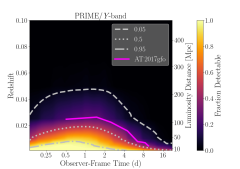
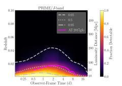
Figure 14: Detectability contours for PRIME (see Figure 9 caption).

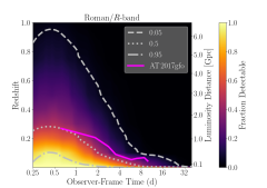
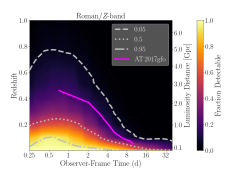
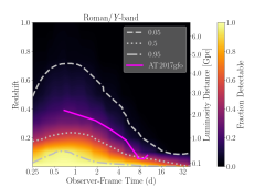
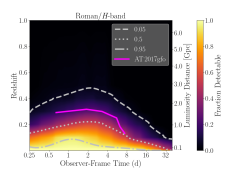
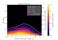
Figure 15: Detectability contours for Roman (see Figure 9 caption).

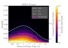
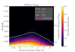
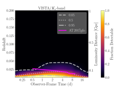
Figure 16: Detectability contours for VISTA (see Figure 9 caption).

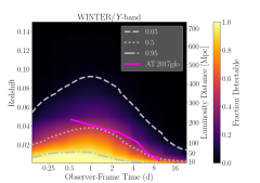
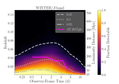
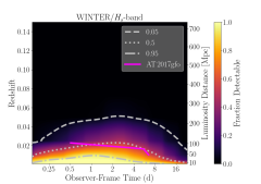
Figure 17: Detectability contours for WINTER (see Figure 9 caption).

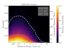
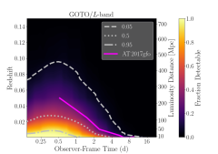
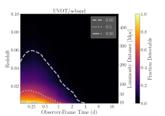
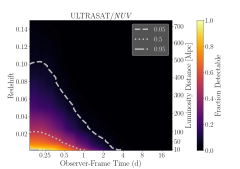
Figure 18: Detectability contours for instruments with only one filter included in the study: DDOTI (top left), GOTO (top right), Swift/UVOT (bottom left), and ULTRASAT (bottom right). See Figure 9 for more details. Note that the range of the vertical axis is not consistent in each panel.

References

- Aasi et al. (2015) Aasi, J., Abbott, B. P., Abbott, R., et al. 2015, Classical and Quantum Gravity, 32, 074001
- Abbott et al. (2017a) Abbott, B. P., Abbott, R., Abbott, T. D., et al. 2017a, Classical and Quantum Gravity, 34, 044001
- Abbott et al. (2017b) —. 2017b, ApJ, 848, L13
- Abbott et al. (2017c) —. 2017c, Phys. Rev. Lett., 119, 161101
- Abbott et al. (2017d) —. 2017d, ApJ, 848, L12
- Abbott et al. (2019) —. 2019, Physical Review X, 9, 031040
- Abbott et al. (2020a) —. 2020a, ApJ, 892, L3
- Abbott et al. (2020b) —. 2020b, Living Reviews in Relativity, 23, 3
- Abbott et al. (2020c) Abbott, R., Abbott, T. D., Abraham, S., et al. 2020c, Phys. Rev. D, 102, 043015
- Abbott et al. (2020d) —. 2020d, ApJ, 896, L44
- Abbott et al. (2020e) —. 2020e, arXiv e-prints, arXiv:2010.14527
- Acernese et al. (2015) Acernese, F., Agathos, M., Agatsuma, K., et al. 2015, Classical and Quantum Gravity, 32, 024001
- Ackley et al. (2020) Ackley, K., Amati, L., Barbieri, C., et al. 2020, A&A, 643, A113
- Akutsu et al. (2019) Akutsu, T., Ando, M., Arai, K., et al. 2019, Nature Astronomy, 3, 35
- Andreoni et al. (2017) Andreoni, I., Ackley, K., Cooke, J., et al. 2017, PASA, 34, e069
- Andreoni et al. (2020) Andreoni, I., Goldstein, D. A., Kasliwal, M. M., et al. 2020, ApJ, 890, 131
- Andreoni et al. (2021) Andreoni, I., Coughlin, M. W., Kool, E. C., et al. 2021, arXiv e-prints, arXiv:2104.06352
- Arcavi (2018) Arcavi, I. 2018, ApJ, 855, L23
- Arcavi et al. (2017) Arcavi, I., Hosseinzadeh, G., Howell, D. A., et al. 2017, Nature, 551, 64
- Artale et al. (2020) Artale, M. C., Bouffanais, Y., Mapelli, M., et al. 2020, MNRAS, 495, 1841
- Ascenzi et al. (2019) Ascenzi, S., Coughlin, M. W., Dietrich, T., et al. 2019, MNRAS, 486, 672
- Astropy Collaboration et al. (2013) Astropy Collaboration, Robitaille, T. P., Tollerud, E. J., et al. 2013, A&A, 558, A33
- Astropy Collaboration et al. (2018) Astropy Collaboration, Price-Whelan, A. M., Sipőcz, B. M., et al. 2018, AJ, 156, 123
- Banerjee et al. (2020) Banerjee, S., Tanaka, M., Kawaguchi, K., Kato, D., & Gaigalas, G. 2020, ApJ, 901, 29
- Banerji et al. (2015) Banerji, M., Jouvel, S., Lin, H., et al. 2015, MNRAS, 446, 2523
- Barbieri et al. (2019) Barbieri, C., Salafia, O. S., Perego, A., Colpi, M., & Ghirlanda, G. 2019, A&A, 625, A152
- Barnes et al. (2016) Barnes, J., Kasen, D., Wu, M.-R., & Martínez-Pinedo, G. 2016, ApJ, 829, 110
- Barnes et al. (2020) Barnes, J., Zhu, Y. L., Lund, K. A., et al. 2020, arXiv e-prints, arXiv:2010.11182
- Bartos et al. (2016) Bartos, I., Huard, T. L., & Márka, S. 2016, ApJ, 816, 61
- Bellm et al. (2019) Bellm, E. C., Kulkarni, S. R., Graham, M. J., et al. 2019, PASP, 131, 018002
- Berger et al. (2013) Berger, E., Fong, W., & Chornock, R. 2013, ApJ, 774, L23
- Blanton et al. (2003) Blanton, M. R., Brinkmann, J., Csabai, I., et al. 2003, AJ, 125, 2348
- Blinnikov et al. (1984) Blinnikov, S. I., Novikov, I. D., Perevodchikova, T. V., & Polnarev, A. G. 1984, Soviet Astronomy Letters, 10, 177
- Bloemen et al. (2015) Bloemen, S., Groot, P., Nelemans, G., & Klein-Wolt, M. 2015, in Astronomical Society of the Pacific Conference Series, Vol. 496, Living Together: Planets, Host Stars and Binaries, ed. S. M. Rucinski, G. Torres, & M. Zejda, 254
- Brown et al. (2013) Brown, T. M., Baliber, N., Bianco, F. B., et al. 2013, PASP, 125, 1031
- Bruni et al. (2021) Bruni, G., O’Connor, B., Matsumoto, T., et al. 2021, MNRAS, arXiv:2105.01440
- Chen et al. (2021) Chen, H.-Y., Holz, D. E., Miller, J., et al. 2021, Classical and Quantum Gravity, 38, 055010
- Chornock et al. (2017) Chornock, R., Berger, E., Kasen, D., et al. 2017, ApJ, 848, L19
- Côté et al. (2018) Côté, B., Fryer, C. L., Belczynski, K., et al. 2018, ApJ, 855, 99
- Coughlin et al. (2018) Coughlin, M. W., Dietrich, T., Doctor, Z., et al. 2018, MNRAS, 480, 3871
- Coughlin et al. (2019) Coughlin, M. W., Ahumada, T., Anand, S., et al. 2019, ApJ, 885, L19
- Coulter et al. (2017) Coulter, D. A., Foley, R. J., Kilpatrick, C. D., et al. 2017, Science, 358, 1556
- Covino et al. (2017) Covino, S., Wiersema, K., Fan, Y. Z., et al. 2017, Nature Astronomy, 1, 791
- Cowperthwaite & Berger (2015) Cowperthwaite, P. S., & Berger, E. 2015, ApJ, 814, 25
- Cowperthwaite et al. (2019) Cowperthwaite, P. S., Villar, V. A., Scolnic, D. M., & Berger, E. 2019, ApJ, 874, 88
- Cowperthwaite et al. (2017) Cowperthwaite, P. S., Berger, E., Villar, V. A., et al. 2017, ApJ, 848, L17
- de Wet et al. (2021) de Wet, S., Groot, P. J., Bloemen, S., et al. 2021, arXiv e-prints, arXiv:2103.02399
- Drout et al. (2017) Drout, M. R., Piro, A. L., Shappee, B. J., et al. 2017, Science, 358, 1570
- Dyer (2020) Dyer, M. J. 2020, PhD thesis, University of Sheffield
- Dyer et al. (2018) Dyer, M. J., Dhillon, V. S., Littlefair, S., et al. 2018, in Society of Photo-Optical Instrumentation Engineers (SPIE) Conference Series, Vol. 10704, Observatory Operations: Strategies, Processes, and Systems VII, 107040C
- Dyer et al. (2020) Dyer, M. J., Steeghs, D., Galloway, D. K., et al. 2020, in Society of Photo-Optical Instrumentation Engineers (SPIE) Conference Series, Vol. 11445, Society of Photo-Optical Instrumentation Engineers (SPIE) Conference Series, 114457G
- Eichler et al. (1989) Eichler, D., Livio, M., Piran, T., & Schramm, D. N. 1989, Nature, 340, 126
- Evans et al. (2016) Evans, P. A., Kennea, J. A., Palmer, D. M., et al. 2016, MNRAS, 462, 1591
- Evans et al. (2017) Evans, P. A., Cenko, S. B., Kennea, J. A., et al. 2017, Science, 358, 1565
- Even et al. (2020) Even, W., Korobkin, O., Fryer, C. L., et al. 2020, ApJ, 899, 24
- Finn & Chernoff (1993) Finn, L. S., & Chernoff, D. F. 1993, Phys. Rev. D, 47, 2198
- Flaugher et al. (2015) Flaugher, B., Diehl, H. T., Honscheid, K., et al. 2015, AJ, 150, 150
- Foley et al. (2019) Foley, R., Bloom, J. S., Cenko, S. B., et al. 2019, BAAS, 51, 305
- Fong et al. (2021) Fong, W., Laskar, T., Rastinejad, J., et al. 2021, ApJ, 906, 127
- Fontes et al. (2020) Fontes, C. J., Fryer, C. L., Hungerford, A. L., Wollaeger, R. T., & Korobkin, O. 2020, MNRAS, 493, 4143
- Fontes et al. (2015) Fontes, C. J., Zhang, H. L., Abdallah, J., J., et al. 2015, Journal of Physics B Atomic Molecular Physics, 48, 144014
- Freiburghaus et al. (1999) Freiburghaus, C., Rosswog, S., & Thielemann, F. K. 1999, ApJ, 525, L121
- Frostig et al. (2020) Frostig, D., Baker, J. W., Brown, J., et al. 2020, in Society of Photo-Optical Instrumentation Engineers (SPIE) Conference Series, Vol. 11447, Society of Photo-Optical Instrumentation Engineers (SPIE) Conference Series, 1144767
- Fryer et al. (1999) Fryer, C. L., Woosley, S. E., & Hartmann, D. H. 1999, ApJ, 526, 152
- Gehrels et al. (2016) Gehrels, N., Cannizzo, J. K., Kanner, J., et al. 2016, ApJ, 820, 136
- Gehrels et al. (2015) Gehrels, N., Spergel, D., & WFIRST SDT Project. 2015, in Journal of Physics Conference Series, Vol. 610, Journal of Physics Conference Series, 012007
- Ghirlanda et al. (2019) Ghirlanda, G., Salafia, O. S., Paragi, Z., et al. 2019, Science, 363, 968
- Goldstein et al. (2017) Goldstein, A., Veres, P., Burns, E., et al. 2017, ApJ, 848, L14
- Goldstein et al. (2020) Goldstein, A., Fletcher, C., Veres, P., et al. 2020, ApJ, 895, 40
- Gompertz et al. (2018) Gompertz, B. P., Levan, A. J., Tanvir, N. R., et al. 2018, ApJ, 860, 62
- Gompertz et al. (2020) Gompertz, B. P., Cutter, R., Steeghs, D., et al. 2020, MNRAS, 497, 726
- Graham et al. (2019) Graham, M. J., Kulkarni, S. R., Bellm, E. C., et al. 2019, PASP, 131, 078001
- Groot (2019) Groot, P. J. 2019, Nature Astronomy, 3, 1160
- Guillochon et al. (2017) Guillochon, J., Parrent, J., Kelley, L. Z., & Margutti, R. 2017, ApJ, 835, 64
- Hall & Evans (2019) Hall, E. D., & Evans, M. 2019, Classical and Quantum Gravity, 36, 225002
- Harris et al. (2020) Harris, C. R., Millman, K. J., van der Walt, S. J., et al. 2020, Nature, 585, 357
- Heinzel et al. (2021) Heinzel, J., Coughlin, M. W., Dietrich, T., et al. 2021, MNRAS, 502, 3057
- Herner et al. (2020) Herner, K., Annis, J., Brout, D., et al. 2020, Astronomy and Computing, 33, 100425
- Hogg et al. (2002) Hogg, D. W., Baldry, I. K., Blanton, M. R., & Eisenstein, D. J. 2002, arXiv e-prints, astro
- Holmbeck et al. (2020) Holmbeck, E. M., Hansen, T. T., Beers, T. C., et al. 2020, ApJS, 249, 30
- Hosseinzadeh et al. (2019) Hosseinzadeh, G., Cowperthwaite, P. S., Gomez, S., et al. 2019, ApJ, 880, L4
- Hotokezaka & Nakar (2020) Hotokezaka, K., & Nakar, E. 2020, ApJ, 891, 152
- Hounsell et al. (2018) Hounsell, R., Scolnic, D., Foley, R. J., et al. 2018, ApJ, 867, 23
- Humason et al. (1956) Humason, M. L., Mayall, N. U., & Sandage, A. R. 1956, AJ, 61, 97
- Hunter (2007) Hunter, J. D. 2007, Computing in Science & Engineering, 9, 90
- Ivezić et al. (2019) Ivezić, Ž., Kahn, S. M., Tyson, J. A., et al. 2019, ApJ, 873, 111
- Jin et al. (2020) Jin, Z.-P., Covino, S., Liao, N.-H., et al. 2020, Nature Astronomy, 4, 77
- Jin et al. (2016) Jin, Z.-P., Hotokezaka, K., Li, X., et al. 2016, Nature Communications, 7, 12898
- Kasen et al. (2015) Kasen, D., Fernández, R., & Metzger, B. D. 2015, MNRAS, 450, 1777
- Kasen et al. (2017) Kasen, D., Metzger, B., Barnes, J., Quataert, E., & Ramirez-Ruiz, E. 2017, Nature, 551, 80
- Kasliwal & Nissanke (2014) Kasliwal, M. M., & Nissanke, S. 2014, ApJ, 789, L5
- Kasliwal et al. (2017) Kasliwal, M. M., Nakar, E., Singer, L. P., et al. 2017, Science, 358, 1559
- Kasliwal et al. (2020) Kasliwal, M. M., Anand, S., Ahumada, T., et al. 2020, ApJ, 905, 145
- King (1952) King, I. 1952, ApJ, 115, 580
- Klingler et al. (2019) Klingler, N. J., Kennea, J. A., Evans, P. A., et al. 2019, ApJS, 245, 15
- Klingler et al. (2021) Klingler, N. J., Lien, A., Oates, S. R., et al. 2021, ApJ, 907, 97
- Korobkin et al. (2012) Korobkin, O., Rosswog, S., Arcones, A., & Winteler, C. 2012, MNRAS, 426, 1940
- Korobkin et al. (2021) Korobkin, O., Wollaeger, R. T., Fryer, C. L., et al. 2021, ApJ, 910, 116
- Kourkchi & Tully (2017) Kourkchi, E., & Tully, R. B. 2017, ApJ, 843, 16
- Kouveliotou et al. (1993) Kouveliotou, C., Meegan, C. A., Fishman, G. J., et al. 1993, ApJ, 413, L101
- Kulkarni (2005) Kulkarni, S. R. 2005, arXiv e-prints, astro
- Lamb et al. (2019) Lamb, G. P., Tanvir, N. R., Levan, A. J., et al. 2019, ApJ, 883, 48
- Lattimer et al. (1977) Lattimer, J. M., Mackie, F., Ravenhall, D. G., & Schramm, D. N. 1977, ApJ, 213, 225
- Lattimer & Schramm (1974) Lattimer, J. M., & Schramm, D. N. 1974, ApJ, 192, L145
- Li & Paczyński (1998) Li, L.-X., & Paczyński, B. 1998, ApJ, 507, L59
- Lippuner et al. (2017) Lippuner, J., Fernández, R., Roberts, L. F., et al. 2017, MNRAS, 472, 904
- Lippuner & Roberts (2015) Lippuner, J., & Roberts, L. F. 2015, ApJ, 815, 82
- Lipunov et al. (2017) Lipunov, V. M., Gorbovskoy, E., Kornilov, V. G., et al. 2017, ApJ, 850, L1
- Lourie et al. (2020) Lourie, N. P., Baker, J. W., Burruss, R. S., et al. 2020, in Society of Photo-Optical Instrumentation Engineers (SPIE) Conference Series, Vol. 11447, Society of Photo-Optical Instrumentation Engineers (SPIE) Conference Series, 114479K
- LVC (2017) LVC. 2017, GRB Coordinates Network, 21513, 1
- LVC (2019) —. 2019, GRB Coordinates Network, 24168, 1
- McMahon et al. (2013) McMahon, R. G., Banerji, M., Gonzalez, E., et al. 2013, The Messenger, 154, 35
- Metzger (2019) Metzger, B. D. 2019, Living Reviews in Relativity, 23, 1
- Metzger et al. (2010) Metzger, B. D., Martínez-Pinedo, G., Darbha, S., et al. 2010, MNRAS, 406, 2650
- Mills et al. (2018) Mills, C., Tiwari, V., & Fairhurst, S. 2018, Phys. Rev. D, 97, 104064
- Möller et al. (1995) Möller, P., Nix, J. R., Myers, W. D., & Swiatecki, W. J. 1995, Atomic Data and Nuclear Data Tables, 59, 185
- Morgan et al. (2020) Morgan, R., Soares-Santos, M., Annis, J., et al. 2020, ApJ, 901, 83
- Narayan et al. (1992) Narayan, R., Paczynski, B., & Piran, T. 1992, ApJ, 395, L83
- Nicholl et al. (2021) Nicholl, M., Margalit, B., Schmidt, P., et al. 2021, arXiv e-prints, arXiv:2102.02229
- Nicholl et al. (2017) Nicholl, M., Berger, E., Kasen, D., et al. 2017, ApJ, 848, L18
- Nissanke et al. (2010) Nissanke, S., Holz, D. E., Hughes, S. A., Dalal, N., & Sievers, J. L. 2010, ApJ, 725, 496
- Nissanke et al. (2013) Nissanke, S., Kasliwal, M., & Georgieva, A. 2013, ApJ, 767, 124
- Norris et al. (1984) Norris, J. P., Cline, T. L., Desai, U. D., & Teegarden, B. J. 1984, Nature, 308, 434
- O’Connor et al. (2021) O’Connor, B., Troja, E., Dichiara, S., et al. 2021, MNRAS, 502, 1279
- Oke & Sandage (1968) Oke, J. B., & Sandage, A. 1968, ApJ, 154, 21
- Paczynski (1986) Paczynski, B. 1986, ApJ, 308, L43
- Page et al. (2020) Page, K. L., Evans, P. A., Tohuvavohu, A., et al. 2020, MNRAS, 499, 3459
- Pankow et al. (2018) Pankow, C., Chase, E. A., Coughlin, S., Zevin, M., & Kalogera, V. 2018, ApJ, 854, L25
- Paterson et al. (2020) Paterson, K., Lundquist, M. J., Rastinejad, J. C., et al. 2020, arXiv e-prints, arXiv:2012.11700
- Perley et al. (2009) Perley, D. A., Metzger, B. D., Granot, J., et al. 2009, ApJ, 696, 1871
- Pian et al. (2017) Pian, E., D’Avanzo, P., Benetti, S., et al. 2017, Nature, 551, 67
- Planck Collaboration et al. (2020) Planck Collaboration, Aghanim, N., Akrami, Y., et al. 2020, A&A, 641, A6
- Popham et al. (1999) Popham, R., Woosley, S. E., & Fryer, C. 1999, ApJ, 518, 356
- Punturo et al. (2010) Punturo, M., Abernathy, M., Acernese, F., et al. 2010, Classical and Quantum Gravity, 27, 194002
- Rastinejad et al. (2021) Rastinejad, J. C., Fong, W., Kilpatrick, C. D., et al. 2021, arXiv e-prints, arXiv:2101.03175
- Ristic et al. (2021) Ristic, M., Champion, E., O’Shaughnessy, R., et al. 2021, arXiv e-prints, arXiv:2105.07013
- Rodrigo & Solano (2020) Rodrigo, C., & Solano, E. 2020, in Contributions to the XIV.0 Scientific Meeting (virtual) of the Spanish Astronomical Society, 182
- Roming et al. (2005) Roming, P. W. A., Kennedy, T. E., Mason, K. O., et al. 2005, Space Sci. Rev., 120, 95
- Rossi et al. (2020) Rossi, A., Stratta, G., Maiorano, E., et al. 2020, MNRAS, 493, 3379
- Rosswog et al. (2017) Rosswog, S., Feindt, U., Korobkin, O., et al. 2017, Classical and Quantum Gravity, 34, 104001
- Sagiv et al. (2014) Sagiv, I., Gal-Yam, A., Ofek, E. O., et al. 2014, AJ, 147, 79
- Savchenko et al. (2017) Savchenko, V., Ferrigno, C., Kuulkers, E., et al. 2017, ApJ, 848, L15
- Schutz (2011) Schutz, B. F. 2011, Classical and Quantum Gravity, 28, 125023
- Scolnic et al. (2018) Scolnic, D., Kessler, R., Brout, D., et al. 2018, ApJ, 852, L3
- Shappee et al. (2017) Shappee, B. J., Simon, J. D., Drout, M. R., et al. 2017, Science, 358, 1574
- Singer et al. (2016) Singer, L. P., Chen, H.-Y., Holz, D. E., et al. 2016, ApJ, 829, L15
- Smartt et al. (2017) Smartt, S. J., Chen, T. W., Jerkstrand, A., et al. 2017, Nature, 551, 75
- Sneden et al. (2009) Sneden, C., Lawler, J. E., Cowan, J. J., Ivans, I. I., & Den Hartog, E. A. 2009, ApJS, 182, 80
- Soares-Santos et al. (2016) Soares-Santos, M., Kessler, R., Berger, E., et al. 2016, ApJ, 823, L33
- Soares-Santos et al. (2017) Soares-Santos, M., Holz, D. E., Annis, J., et al. 2017, ApJ, 848, L16
- Spergel et al. (2015) Spergel, D., Gehrels, N., Baltay, C., et al. 2015, arXiv e-prints, arXiv:1503.03757
- Sutherland et al. (2015) Sutherland, W., Emerson, J., Dalton, G., et al. 2015, A&A, 575, A25
- Symbalisty & Schramm (1982) Symbalisty, E., & Schramm, D. N. 1982, Astrophys. Lett., 22, 143
- Tanvir et al. (2013) Tanvir, N. R., Levan, A. J., Fruchter, A. S., et al. 2013, Nature, 500, 547
- Tanvir et al. (2017) Tanvir, N. R., Levan, A. J., González-Fernández, C., et al. 2017, ApJ, 848, L27
- Thakur et al. (2020) Thakur, A. L., Dichiara, S., Troja, E., et al. 2020, MNRAS, 499, 3868
- Troja et al. (2017) Troja, E., Piro, L., van Eerten, H., et al. 2017, Nature, 551, 71
- Troja et al. (2018) Troja, E., Ryan, G., Piro, L., et al. 2018, Nature Communications, 9, 4089
- Troja et al. (2019a) Troja, E., van Eerten, H., Ryan, G., et al. 2019a, MNRAS, 489, 1919
- Troja et al. (2019b) Troja, E., Castro-Tirado, A. J., Becerra González, J., et al. 2019b, MNRAS, 489, 2104
- Utsumi et al. (2017) Utsumi, Y., Tanaka, M., Tominaga, N., et al. 2017, PASJ, 69, 101
- Valenti et al. (2017) Valenti, S., Sand, D. J., Yang, S., et al. 2017, ApJ, 848, L24
- Virtanen et al. (2020) Virtanen, P., Gommers, R., Oliphant, T. E., et al. 2020, Nature Methods, 17, 261
- Watson et al. (2016) Watson, A. M., Lee, W. H., Troja, E., et al. 2016, in Society of Photo-Optical Instrumentation Engineers (SPIE) Conference Series, Vol. 9910, Observatory Operations: Strategies, Processes, and Systems VI, ed. A. B. Peck, R. L. Seaman, & C. R. Benn, 99100G
- Winteler et al. (2012) Winteler, C., Käppeli, R., Perego, A., et al. 2012, ApJ, 750, L22
- Wollaeger & van Rossum (2014) Wollaeger, R. T., & van Rossum, D. R. 2014, ApJS, 214, 28
- Wollaeger et al. (2013) Wollaeger, R. T., van Rossum, D. R., Graziani, C., et al. 2013, ApJS, 209, 36
- Wollaeger et al. (2018) Wollaeger, R. T., Korobkin, O., Fontes, C. J., et al. 2018, MNRAS, 478, 3298
- Wollaeger et al. (2021) Wollaeger, R. T., Fryer, C. L., Chase, E. A., et al. 2021, ApJ, submitted
- Yang et al. (2015) Yang, B., Jin, Z.-P., Li, X., et al. 2015, Nature Communications, 6, 7323
- Zhu et al. (2021) Zhu, Y. L., Lund, K. A., Barnes, J., et al. 2021, ApJ, 906, 94