Euler-Schrödinger Transformation

Abstract

Here we present a transformation that maps the Schrödinger equation of quantum mechanics to the incompressible Euler equations of fluid mechanics. The transformation provides a wave solution and a potential function based on fluid properties that satisfy the Schrödinger equation given that the fluid velocity and pressure satisfy the Euler equations. Interestingly, in our transformation, the equivalent of quantum potential becomes the physical surface tension. This is contrary to the Madelung transformation that maps the Schrödinger equation to the compressible Euler equations where there is no physical counterpart for the quantum potential. Lastly, we show that using this transformation, the Bohm equation can be mapped to a particle’s equation of motion moving on the free surface of the fluid.

We present a transformation between the Schrödinger equation of quantum mechanics and the incompressible Euler equations (incompressible, inviscid, and irrotational hydrodynamic equations for the surface gravity waves). It is to be noted that the transformation between the Schrödinger equation and compressible Euler equations is known as the Madelung transform. Contrary to the Madelung transformation where there is no classical analog for the quantum potential, we find a classical counterpart to the quantum potential which becomes the surface tension with the Planck constant acting similar to the surface tension over density. We present two versions of our transformation, where we add complexity to the transformation step by step: (i) in the first version, we map the Schrödinger equation to the surface gravity wave equations for an inviscid, irrotational, and incompressible fluid with surface tension in deep water; (ii) next, we assume a finite depth fluid and also a particle bouncing on the free surface (bouncind droplet setup Couder et al. (2005)), and show how the transformation changes in mapping Schrödinger equation to the Euler equations. Assuming Bohmian mechanics, we find the analog of Bohm equation using our transformation, and show that under certain conditions, the transformation of Bohm equation matches with the Newton equation of motion for the bouncing droplet. This process may help us understand why the bouncing droplet problem Couder et al. (2005) has shown quantum resemblance (such as single-slit patterns and double-slit diffraction Couder and Fort (2006), tunnelling Eddi et al. (2009), orbital quantization Fort et al. (2010), level splitting Eddi et al. (2012), and wavelike statistics in a confined region Harris et al. (2013)).

I (I) Simplified Euler-Schrödinger Transformation

Schrödinger equation– The position-space Schrödinger equation for a single non-relativistic particle with mass $m$ in a potential $V(\textbf{q},t)$ is

$$\mathrm{i}\hbar\frac{\partial\psi}{\partial t}(\textbf{q},t)=-\frac{\hbar^{2}}{2m}\Delta\psi(\textbf{q},t)+V(\textbf{q})\psi(\textbf{q},t)$$ (1)

where $\hbar$ is the reduced Planck constant ($\hbar=h/2\pi$), and $\psi(\textbf{q},t):\mathbb{R}^{3}\times\mathbb{R}\rightarrow\mathbb{C}$ is a wave function that assigns a complex number to each point $\textbf{q}\in\mathbb{R}^{3}$ in space at each time $t\in\mathbb{R}$.

Euler equations– Considering the irrotational motion of a homogeneous, incompressible, and inviscid fluid with the surface tension $\sigma$ and density $\rho$; the governing equations in terms of the velocity potential $\phi$ and surface elevation $\eta$ read

$$\nabla^{2}\phi=0,\qquad z\leq\eta,$$ (2a)

$$\eta_{t}+\nabla(\eta-z).\nabla\phi=0,\qquad z=\eta,$$ (2b)

$$\phi_{t}+\frac{1}{2}|\nabla\phi|^{2}+g\eta+\frac{\sigma}{\rho}\nabla.\hat{\textbf{n}}=0\qquad z=\eta,$$ (2c)

$$\phi_{z}=0,\qquad z\rightarrow-\infty,$$ (2d)

where $\hat{\textbf{n}}$ is the unit normal vector at the surface $z=\eta$. In the governing equations, (2a) is the continuity equation in the fluids domain, (2b) and (2d) are kinematic boundary conditions at the surface and bottom, and (2c) is the dynamic boundary condition at the surface.

The Euler-Schrödinger Transformation– In the Schrödinger equation, we pick $m=1$, $\hbar=\sqrt{{2\sigma}/{\rho}}$ and define the potential function as $V=\frac{1}{\hbar}\left(P/\rho+gz\right)$, where the parameters are related to the fluid equations of motion. We assume a wave function in the form of $\Psi=H(\eta-z)\exp\left({\mathrm{i}\phi/\hbar}\right)$, where $H(\cdot)$ is a step function (see Fig. 1).

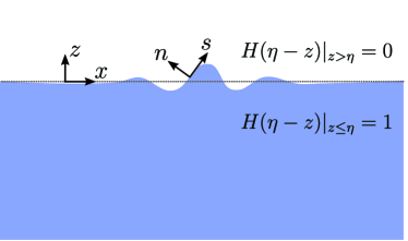
Figure 1: Schematic of an incompressible fluid with a free surface. The calm fluid surface is at $z=0$ and positive $z$ points upward. The tangential and normal coordinate system is defined on the free surface, where positive $n$ points outward. The step functions are unity inside the fluids domain $\mathcal{H}=H(\eta-z)|_{z<\eta}=1$, and zero outsize $H(\eta-z)|_{z>\eta}=0$.

Next, we show that if $\Psi=H(\eta-z)\exp\left({\mathrm{i}\phi/\hbar}\right)$ satisfies the Schrödinger’s equation (Eq.(1)) with $V=\frac{1}{\hbar}\left(P/\rho+gz\right)$, the fluid properties $\eta,\phi,\rho,P$ should then satisfy the Euler equations (Eq. (2)). Inserting the wave function into the Schrödinger equation (1), we obtain the following equations for the real and imaginary part:

$$-H(\eta-z)\phi_{t}+\frac{\sigma}{\rho}\nabla^{2}H(\eta-z)-\frac{1}{2}H(\eta-z)|\nabla\phi|^{2}$$

$$\qquad-\left(\frac{P}{\rho}+gz\right)\cdot H(\eta-z)=0,$$ (3a)

$$\mathrm{i}\left(\frac{\partial}{\partial t}H(\eta-z)+\nabla H(\eta-z)\cdot\nabla\phi\right)+\mathrm{i}\frac{1}{2}H(\eta-z)\nabla^{2}\phi=0.$$ (3b)

Here Eq. (3a) is the real part and Eq. (3b) is the imaginary part. Note that $F(x,y,z):=\eta(x,y)-z=0$ defines the free water surface $\Gamma_{s}$, and as a result $\partial H(\eta-z)/\partial t=\eta_{t}\delta(\eta-z)$, and $\nabla H(\eta-z)=\nabla(\eta-z)\delta(\eta-z)$. We now show that Eqs. (3)a-d is equivalent to Eq. (2). Multiplying Eq. (3b) by an arbitrary function $f(\textbf{x})$ where $\textbf{x}\in\mathbb{R}^{3}$ and integrating over the whole space $\Omega\subseteq\mathbb{R}^{3}$, we obtain

$$\iiint_{\Omega}\left[f(\mathbf{x})\left(\eta_{t}+\nabla(\eta-z).\nabla\phi\right)\right]\delta(\eta-z)\textrm{d}V$$

$$\qquad+\iiint_{\Omega}\frac{1}{2}H(\eta-z)f(\mathbf{x})\nabla^{2}\phi\textrm{d}V=0,$$ (4)

which reduces to

$$\iint_{\mathcal{S}}\left[f(\mathbf{x})\left(\eta_{t}+\nabla(\eta-z).\nabla\phi\right)\right]_{z=\eta}\textrm{d}A$$

$$\qquad+\iint_{\mathcal{S}}\textrm{d}A\int_{-\infty}^{\eta}\textrm{d}zf(\mathbf{x})\nabla^{2}\phi=0,$$ (5)

where $\mathcal{S}\subseteq\mathbb{R}^{2}$ is the free surface of the fluid. Since $f(\mathbf{x})$ is an arbitrary function, we obtain

$$\nabla^{2}\phi=0,\qquad-\infty\leq z\leq\eta$$ (6a)

$$\eta_{t}+\nabla(\eta-z).\nabla\phi=0\qquad z=\eta$$ (6b)

which are respectively the incompressibility and the kinematic boundary conditions. We now show that (3a) simplifies to the dynamic boundary condition (2c). Let $g(\mathbf{x})$ be a function with supp$(g)=\mathbb{R}^{2}\times[a,b]$, where $a<\inf(\eta)-\delta<0$, $b>\sup(\eta)+\delta$, and $\delta>0$. We assume the normal derivative of this function on the surface is zero, i.e. $\partial g/\partial n|_{z=\eta}=0$, where n is the normal direction on the surface $z=\eta$. We now multiply equation (3a) by this function $g(\mathbf{x})$ and take the integral over $\Omega=\mathbb{R}^{2}\times[a^{\prime},b^{\prime}]$, where in the $z$-direction it contains supp$(g)$, i.e. $a^{\prime}\leq a\leq 0\leq b\leq b^{\prime}$. We find

$$\iiint_{\Omega}H(\eta-z)g(\mathbf{x})\left(\phi_{t}+\frac{1}{2}|\nabla\phi|^{2}+\frac{P}{\rho}+g\right)\textrm{d}V$$

$$\qquad-\frac{\sigma}{\rho}\iiint_{\Omega}g(\mathbf{x})\nabla\ \cdot\left(-\textbf{n}\delta(n)\right)=0,$$ (7)

where we used the fact that $\nabla H(\eta-z)=-\hat{\textbf{n}}~{}\delta(n)$. Expanding the right hand side, we obtain

$$\iint_{\mathcal{S}}\textrm{d}A\int_{a^{\prime}}^{\eta}\textrm{d}zg(\mathbf{x})\left(\phi_{t}+\frac{1}{2}|\nabla\phi|^{2}+\frac{P}{\rho}+g\right)$$

$$+\frac{\sigma}{\rho}\left[\iiint_{\Omega}\left(g(\mathbf{x})\nabla\cdot\hat{\textbf{n}}\delta(n)+g(\mathbf{x})\frac{\partial}{\partial n}\delta(n)\right)\textrm{d}V\right]=0.$$ (8)

and as a result

$$\iint_{\mathcal{S}}\textrm{d}A\int_{a^{\prime}}^{\eta}\textrm{d}zg(\mathbf{x})\left(\phi_{t}-\frac{1}{2}|\nabla\phi|^{2}+\frac{P}{\rho}+g\right)$$

$$\quad+\frac{\sigma}{\rho}\iiint_{\Omega}g(\mathbf{x})\nabla\cdot\hat{\textbf{n}}\delta(n)\,\textrm{d}V=-\frac{\sigma}{\rho}\iiint_{\Omega}g(\mathbf{x})\frac{\partial}{\partial n}\delta(n)\,\textrm{d}V.$$ (9)

The right-hand side of the above equation is zero: if we use integral by parts on the right-hand side, we obtain

$$\iiint_{\Omega}g(\mathbf{x})\frac{\partial}{\partial n}\delta(n)\textrm{d}V$$

$$\qquad=\iiint_{\Omega}\frac{\partial}{\partial n}\left(g(\mathbf{x})\delta(n)\right)\textrm{d}V-\iiint_{\Omega}\left(\frac{\partial g(\mathbf{x})}{\partial n}\right)\delta(n)\,\textrm{d}V,$$ (10)

where (i) the first and (ii) the second integrals are zero, since (i) by changing the coordinates from Cartesian coordinate $(x,y,z)$ to $(t,s,n)$, this integral vanishes with the compactness of $g(\mathbf{x})$ and (ii) we assumed that $\partial g/\partial n|_{z=\eta}=0$. Looking back at Eq. (I), since $g(\mathbf{x})$ is arbitrary, we obtain

$$\phi_{t}-\frac{1}{2}|\nabla\phi|^{2}+\frac{P}{\rho}+gz+\left(\frac{\sigma}{\rho}\nabla.\textbf{n}\right)\delta(n)=0,\quad z\leq\eta$$ (11)

which is the same as equation (2c) on the surface. Note that Eq. (11) is what we obtain starting from Navier-Stokes equations, and in the Euler equations we only consider the above equation on the free surface, i.e., $z=\eta$. Equations (6) and (11) together are collectively the Euler equations (Eq. (2)). Note that, since the domain is unbounded in the $z$-direction, we impose the regularizing condition that $\phi$ vanishing at infinity (i.e., $z\rightarrow\infty$), which is Eq. (2d) and is a condition for the velocity potential to be bounded.

II (II) Euler-Schrödinger transformation

Schrödinger equation– As discussed in the previous section, the Schrödinger equation is

$$\mathrm{i}\hbar\frac{\partial\psi}{\partial t}(\textbf{x},t)=-\frac{\hbar^{2}}{2m}\Delta\psi(\textbf{x},t)+V(\textbf{x})\psi(\textbf{x},t),$$ (12)

where $\hbar$ is the reduced Plank constant, and $\psi(\textbf{x},t):\mathbb{R}^{3}\times\mathbb{R}\rightarrow\mathbb{C}$ is the wave function of a particle with mass $m$ in the potential $V(\textbf{x})$. Considering Bohmian mechanics, there exists a particle with mass $m$ and position $\textbf{Q}\in\mathbb{R}^{3}$, and the particle is guided by a the wave function $\psi(\textbf{x},t)$ with the equation

$$\frac{\textrm{d}\textbf{Q}}{\textrm{d}t}=\frac{\hbar}{m}\Im\left\{\frac{\nabla\psi}{\psi}(\textbf{x},t)\right\},$$ (13)

where $\Im(z)$ gives the imaginary part of the complex number $z$. This equation is known as Bohm equation, and governs the trajectory of a quantum particle.

Euler’s equations– Now consider a fluid bath with a free surface on a vibrating plate where a droplet is bouncing on its free surface (see Fig. 2). We assume a coordinate system attached to the vibrating bath with a positive $z$-axis pointing upward and the fluid’s calm surface being at $z=0$. The vibration frequency of the bath is identified by $\omega$ and the acceleration amplitude is $\gamma$ i.e. the acceleration is $\hat{\gamma}=\gamma\cos(\omega t)$. We consider the fluid to be homogeneous, incompressible, inviscid, and irrotational. At each time the droplet hits the surface, it receives some force $\vec{\mathcal{F}}_{i}$ at the particle’s location $\textbf{X}_{i}$ and impacts time $t_{i}$. Since $\vec{\mathcal{F}}_{i}$ is the contact force applied to the droplet, $-\vec{\mathcal{F}}_{i}$ is the reaction of this force and is applied to the fluid surface. The governing equations for the fluid read as

$$\nabla^{2}\phi=0,\qquad z\leq\eta,$$ (14a)

$$\eta_{t}+\nabla(\eta-z).\nabla\phi=0,\qquad z=\eta,$$ (14b)

$$\phi_{t}+\frac{1}{2}|\nabla\phi|^{2}+(g-\hat{\gamma})\eta+\frac{\sigma}{\rho}\nabla.\hat{\textbf{n}}+$$

$$\qquad\sum_{i}\Theta_{i}\delta(\textbf{x}-\textbf{X}_{i})\delta(t-t_{i})=0\qquad z=\eta,$$ (14c)

$$\phi_{z}=0,\qquad z=-h,$$ (14d)

where $z=-h$ is the bottom of the fluid bath, $\hat{\textbf{n}}$ is unit normal vector at the surface $z=\eta$, and $\Theta_{i}$ is a potential function defined as $\vec{\mathcal{F}}_{i}=-\nabla\Theta_{i}$. Here, (14a) is the continuity equation in the fluid domain, (14b) and (14d) are kinematic boundary conditions at the free surface and bottom boundary, and (14c) is the dynamic boundary condition at the surface. The Euler equations (Eqs. (14)a-d) and droplet’s equation are coupled, and should be solved together. The droplet’s equation of motion can be written as

$$m\frac{\textrm{d}^{2}\textbf{X}}{\textrm{d}t^{2}}=-m(g-\hat{\gamma})\,\hat{\mathbf{z}}+\sum_{i}\vec{\mathcal{F}}_{i}\delta(\textbf{x}-\textbf{X}_{i})\delta(t-t_{i}),$$ (15)

where $m$ is the mass of the droplet, X is its position vector of the droplet, $\vec{\mathcal{F}}_{i}$ accounts for the contact force applied to the particle at time $t_{i}$ and the particle’s location $\textbf{X}_{i}$, and $\delta(\cdot)$ is the Dirac delta function. It is worth noting that, in the Eqs. (14)a-d, if we set all $\vec{\mathcal{F}}_{i}=0$, and also $\hat{\gamma}=0$, the governing equations reduce to general Euler equations (Eqs. (2)a-d).

Euler-Schrödinger Transformation– In this section, we present a wave function $\Psi$ and a potential function $V$ as a function of fluid free surface $\eta$, and velocity potential $\phi$, such that if $\Psi$ and $V$ satisfy the Schrödinger equation (Eq. (12)) then the resulting $\eta$ and $\phi$ satisfy the Euler equations (Eqs. (14)a-d). Conversely, if $\eta$ and $\phi$ satisfy the Euler equations, the obtained wave function $\Psi$ satisfies the Schrödinger equation with the potential function $V$.

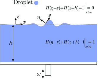
Figure 2: Schematic of the fluid bath and droplet bouncing on its free surface. The calm fluid surface is at $z=0$ with positive $z$ pointing upward. The tangential coordinate is defined on the surface with positive normal direction $n$ points out of the fluid’s domain. The step function $\left[H(\eta-z)+H(z+h)-1\right]|_{-h<z<\eta}=1$ inside the fluid and $\left[H(\eta-z)+H(z+h)-1\right]|_{z>\eta}=0$ outside of the fluid domain. The fluid depth is $\tilde{h}$.

Consider a wave function as

$$\Psi\equiv\left[H(\eta-z)+H(z+h)-1\right]\exp(\mathrm{i}\phi/\hbar),$$ (16)

where $H(\cdot)$ is a step function, and $z=-h$ represents the bottom of the fluid bath. Additionally, we define a potential function $V$ in the Schrödinger equation based on the fluids parameters as

$$V\equiv\frac{1}{\hbar}\left(P/\rho+(g-\hat{\gamma})z+\sum\Theta_{i}\delta(\textbf{x}-\textbf{X}_{i})\delta(t-t_{i})\right),$$ (17)

and assume $m\equiv 1$, $\hbar\equiv\sqrt{2\sigma/\rho}$. Inserting the wave function into the Schrödinger equation, we obtain

$$\mathrm{i}\left(\frac{\partial}{\partial t}H(\eta-z)+\nabla H(\eta-z).\nabla\phi\right)+$$

$$\quad\mathrm{i}\left(\frac{\partial}{\partial t}H(z+h)+\nabla H(z+h).\nabla\phi\right)+$$

$$\qquad\quad\mathrm{i}\frac{1}{2}\left[H(\eta-z)+H(z+h)-1\right]\nabla^{2}\phi=0,$$ (18)

for the imaginary part, and for the real part we obtain

$$-\left[H(\eta-z)+H(z+h)-1\right]\phi_{t}+\frac{\sigma}{\rho}\nabla^{2}H(\eta-z)$$

$$\quad+\frac{\sigma}{\rho}\nabla^{2}H(z+h)-\left[H(\eta-z)+H(z+h)-1\right]\cdot$$

$$\left(\frac{1}{2}|\nabla\phi|^{2}+\frac{P}{\rho}+(g-\hat{\gamma})z+\sum\Theta_{i}\delta(\textbf{x}-\textbf{X}_{i})\delta(t-t_{i})\right)=0.$$ (19)

Note that Eqs. (II) and (II) here are similar to the Eqs. (3b) and (3a). Equation (II) can be simplified to

$$\mathrm{i}\left(\frac{\partial\eta}{\partial t}+\nabla(\eta-z).\nabla\phi\right)\delta(\eta-z)+\mathrm{i}\left(\hat{\mathbf{z}}.\nabla\phi\right)\delta(z+h)+$$

$$\qquad\quad\mathrm{i}\frac{1}{2}\left[H(\eta-z)+H(z+h)-1\right]\nabla^{2}\phi=0.$$ (20)

With an argument, similar to that of the previous section, this equation reduces to

$$\nabla^{2}\phi=0,\quad-h\leq z\leq\eta,$$ (21a)

$$\eta_{t}+\nabla(\eta-z).\nabla\phi=0,\quad z=\eta,$$ (21b)

$$\phi_{z}=0,\qquad z=-h,$$ (21c)

where equations (21a), (21b), (21c) matches with equations (14a), (14b), (14d) respectively. Furthermore, equation (II), with an argument similar to that of the previous section, reduces to

$$\phi_{t}+\frac{1}{2}|\nabla\phi|^{2}+(g-\hat{\gamma})z+$$

$$\qquad\sum\Theta_{i}\delta(\textbf{x}-\textbf{X}_{i})\delta(t-t_{i})+\left(\frac{\sigma}{\rho}\nabla.\textbf{n}\right)=0,\quad z=\eta,$$ (22a)

$$\phi_{t}+\frac{1}{2}|\nabla\phi|^{2}+\frac{P}{\rho}+(g-\hat{\gamma})z+$$

$$\quad\sum\Theta_{i}\delta(\textbf{x}-\textbf{X}_{i})\delta(t-t_{i})=0,\quad-h\leq z<\eta,$$ (22b)

which at $z=\eta$ matches with equation (14c). Note that the fluid pressure becomes zero at the fluid’s free surface, i.e., $P_{z=\eta}=0$.

Particle’s Motion– Inserting the wave function (16) into the Bohm equation (13), we obtain

$$\textbf{v}=\frac{\textrm{d}\textbf{Q}}{\textrm{d}t}=\nabla\phi.$$ (23)

Note that in our droplet’s setup, the droplet is outside the fluid, while $\phi$ is only defined at the surface and inside the fluid domain. We, therefore, take $\phi$ as the velocity potential calculated at the surface. Taking the time derivative of equation (23), the particle’s dynamic equation is obtained. Using (14b), the acceleration of the particle becomes

$$\frac{\textrm{d}\textbf{v}}{\textrm{d}t} =\nabla\phi_{t}=\nabla\left(\frac{1}{2}|\nabla\phi|^{2}\right)-(g-\hat{\gamma})\,\hat{\mathbf{z}}+$$

$$\sum\vec{\mathcal{F}}_{i}\delta(\textbf{x}-\textbf{X}_{i})\delta(t-t_{i})+\nabla\left(\frac{\sigma}{\rho}\nabla.\textbf{n}\right).$$ (24)

Assuming the non-linearity is small i.e. $|\nabla\phi|/|\textbf{v}|\ll 1$, the droplet’s equation of motion becomes

$$\frac{\textrm{d}\textbf{v}}{\textrm{d}t}=-(g-\hat{\gamma})\,\hat{\mathbf{z}}+\sum\vec{\mathcal{F}}\delta(\textbf{x}-\textbf{X}_{i})\delta(t-t_{i})+\nabla\left(\frac{\sigma}{\rho}\nabla.\textbf{n}\right).$$ (25)

The obtained equation is similar to (15) with an extra term on the right-hand side, that is related to the gradient effect of surface tension.

III Remarks

In this section, we review some basic conclusions that can be made based on the transformation.

• The probability of finding a particle at a point is proportional to $|\psi|^{2}$ and the integral of this probability over the whole space should add up to unity

  $$\int|\psi|^{2}\textrm{d}V=1.$$ (26)

  The equivalent of this condition, using the transformation, translates into the fact that the volume of the fluid is constant,

  $$\int H(\eta-z)\cdot H(\eta-z)\textrm{d}V=\int_{\Lambda}\textrm{d}V=V_{0},$$ (27)

  where $\Lambda$ is the fluids domain and $V_{0}$ is the total volume of fluid.

• The flow of probability using the Schrödinger equation is obtained as

  $$\frac{\partial|\psi|^{2}}{\partial t}+\nabla.\left[\frac{\hbar}{2m\mathrm{i}}\left(\psi^{*}\nabla\psi-\psi\nabla\psi^{*}\right)\right]=0.$$ (28)

  The equivalent form of this equation, using the Euler-Schrödinger equation becomes

  $$\qquad\frac{\partial H(\eta-z)\cdot H(\eta-z)}{\partial t}+$$

  $$\qquad\quad\quad\frac{1}{2}\nabla.(H(\eta-z)\cdot H(\eta-z)\nabla\phi)=0,$$ (29)

  $$\qquad\delta(\eta-z)\left[\eta_{t}+\nabla(\eta-z).\nabla\phi\right]+$$

  $$\qquad\quad\quad\frac{1}{2}H(\eta-z)\nabla^{2}\phi=0,$$ (30)

  which is the same as surface kinematic boundary condition together with the Laplacian equation (conservation of mass).

• The scale at which quantum effects are observed is such that $\hbar/ML^{2}T^{-1}\approx 1$, where $M,L$, and $T$ are the mass, length and time scales of the problem. Similar arguments for the bouncing droplet’s problem, yield $\sigma/\rho gL^{2}\approx 1$. As a result, the length scale at which we expect to see quantum-like behaviors for the silicone oil becomes $L\approx 2.5mm$, which is close to the length scale of experiments.

IV Conclusion

In summary, we provided a transformation that maps the Schrödinger equation of quantum wave mechanics to Euler equations of fluid wave mechanics. Specifical,ly we showed

Schrödinger Equation: $$\qquad\mathrm{i}\hbar\frac{\partial\psi}{\partial t}(\textbf{x},t)=-\frac{\hbar^{2}}{2m}\Delta\psi(\textbf{x},t)+V(\textbf{x})\psi(\textbf{x},t)$$ (31)

$$\text{Assuming:}\quad\Bigg{\updownarrow} \psi(\textbf{x},t)=\left[H(\eta-z)+H(z+h)-1\right]e^{\mathrm{i}\phi/\hbar},~{}V=\frac{1}{\hbar}\left(\frac{P}{\rho}+gz\right)$$ (32)

Euler’s Equation: $$\qquad\begin{cases}&\nabla^{2}\phi=0,\qquad-h\leq z\leq\eta\\ &\eta_{t}+\nabla(\eta-z).\nabla\phi=0,\qquad z=\eta\\ &\phi_{t}+\frac{1}{2}|\nabla\phi|^{2}+g\eta+\frac{\sigma}{\rho}\nabla.\hat{\textbf{n}}=0\\ &\phi_{z}=0,\qquad z=-h\end{cases}$$ (33)

wherein (31), $\psi$ is the wave function, $\hbar$ is the reduced Plank constant, and $m$ is the quantum particle’s mass; and in (33), $\phi$ is the velocity potential, $z=\eta$ is the free surface, $\rho$ is fluid’s density, $\sigma$ is the surface tension, and n is the a normal vector pointing outward of the fluid’s free surface at $z=\eta$. Equation (32) also provides the transformation that relates the quantum wave solution and potential to the fluid’s parameters. We further showed that the same transformation works even when the fluid bath is vibrating with the acceleration $\gamma=\hat{\gamma}\cos\omega t$ and there is a particle that bounces on the surface and exerts a force at the surface $\mathcal{F}_{i}=\nabla\Theta_{i}$ at the point $\textbf{x}=\textbf{X}_{i}$ and time $t=t_{i}$. Precisely the equations are

Schrödinger Equation: $$\qquad\mathrm{i}\hbar\frac{\partial\psi}{\partial t}(\textbf{x},t)=-\frac{\hbar^{2}}{2m}\Delta\psi(\textbf{x},t)+V(\textbf{x})\psi(\textbf{x},t)$$

$$\text{Assuming:}\quad\Bigg{\uparrow} \psi(\textbf{x},t)=\left[H(\eta-z)+H(z+h)-1\right]e^{\mathrm{i}\phi/\hbar},$$

$$\text{and}\quad\quad\Bigg{\downarrow} ~{}V=\frac{1}{\hbar}\left(\frac{P}{\rho}+(g-\hat{\gamma})z+\sum\Theta_{i}\delta(\textbf{x}-\textbf{X}_{i})\delta(t-t_{i})\right)$$

Euler’s Equation: $$\qquad\begin{cases}&\nabla^{2}\phi=0,\qquad-h\leq z\leq\eta\\ &\eta_{t}+\nabla(\eta-z).\nabla\phi=0,\qquad z=\eta\\ &\phi_{t}+\frac{1}{2}|\nabla\phi|^{2}+(g-\hat{\gamma})\eta+\frac{\sigma}{\rho}\nabla.\hat{\textbf{n}}+\sum_{i}\Theta_{i}\delta(\textbf{x}-\textbf{X}_{i})=0\\ &\phi_{z}=0,\qquad z=-h\end{cases}$$

Considering this transformation, the Bohm particle equation also maps to the particle’s equation of motion if the surface remains almost flat and we can ignore the nonlinear term, i.e.,

$$\frac{\textrm{d}\textbf{Q}}{\textrm{d}t}=\frac{\hbar}{m}\Im\left\{\frac{\nabla\psi}{\psi}(\textbf{x},t)\right\}$$

$$\qquad\qquad\big{\downarrow}$$

$$m\frac{\textrm{d}^{2}\textbf{X}}{\textrm{d}t^{2}}=-m(g-\gamma)\hat{\mathbf{z}}+\sum\vec{\mathcal{F}}_{i}\delta(\textbf{x}-\textbf{X}_{i})\delta(t-t_{i})$$

References

- Couder et al. (2005) Y. Couder, S. Protiere, E. Fort, and A. Boudaoud, Nature 437, 208 (2005).
- Couder and Fort (2006) Y. Couder and E. Fort, Physical review letters 97, 154101 (2006).
- Eddi et al. (2009) A. Eddi, E. Fort, F. Moisy, and Y. Couder, Physical review letters 102, 240401 (2009).
- Fort et al. (2010) E. Fort, A. Eddi, A. Boudaoud, J. Moukhtar, and Y. Couder, Proceedings of the National Academy of Sciences 107, 17515 (2010).
- Eddi et al. (2012) A. Eddi, J. Moukhtar, S. Perrard, E. Fort, and Y. Couder, Physical review letters 108, 264503 (2012).
- Harris et al. (2013) D. M. Harris, J. Moukhtar, E. Fort, Y. Couder, and J. W. Bush, Physical Review E 88, 011001 (2013).