Imaging in random media by two-point coherent interferometry

Liliana Borcea111Department of Mathematics, University of Michigan, Ann Arbor, MI 48109. borcea@umich.edu    Josselin Garnier222CMAP, CNRS, Ecole Polytechnique, Institut Polytechnique de Paris, 91128 Palaiseau Cedex, France. josselin.garnier@polytechnique.edu
Abstract

This paper considers wave-based imaging through a heterogeneous (random) scattering medium. The goal is to estimate the support of the reflectivity function of a remote scene from measurements of the backscattered wave field. The proposed imaging methodology is based on the coherent interferometric (CINT) approach that exploits the local empirical cross correlations of the measurements of the wave field. The standard CINT images are known to be robust (statistically stable) with respect to the random medium, but the stability comes at the expense of a loss of resolution. This paper shows that a two-point CINT function contains the information needed to obtain statistically stable and high-resolution images. Different methods to build such images are presented, theoretically analyzed and compared with the standard imaging approaches using numerical simulations. The first method involves a phase-retrieval step to extract the reflectivity function from the modulus of its Fourier transform. The second method involves the evaluation of the leading eigenvector of the two-point CINT imaging function seen as the kernel of a linear operator. The third method uses an optimization step to extract the reflectivity function from some cross products of its Fourier transform. The presentation is for the synthetic aperture radar data acquisition setup, where a moving sensor probes the scene with signals emitted periodically and records the resulting backscattered wave. The generalization to other imaging setups, with passive or active arrays of sensors, is discussed briefly.

keywords:
Imaging, wave scattering, random medium, coherent interferometry, synthetic aperture radar, spectral analysis, phase retrieval.
AMS:
35Q93, 45Q05, 49R99, 60H30.

1 Introduction

The goal of inverse scattering is to estimate an unknown medium using sensors that emit probing signals and measure the generated (backscattered or transmitted) waves. The mathematical formulation is an inverse problem for a wave equation, that seeks to “invert” the nonlinear mapping between the unknown coefficients (e.g. wave speed) and the solution (the wave) at the points of measurement. Typically the mapping is not invertible, hence the quotation marks, and only an approximation of the coefficients can be expected.

Wave-based imaging is a simplification of the inverse scattering problem, which seeks a qualitative estimate of the reflective structures in the medium, modeled by a reflectivity function ρ𝜌\rho which captures sharp variations (e.g., jump discontinuities) of the coefficients in the wave equation. It uses various data processing to compute an imaging function (image in short) (y)y\mathcal{I}({{\itbf y}}) at points yy{{\itbf y}} in a search region, whose peaks are interpreted as locations of the sought-after reflectors.

The existing imaging methodology has been driven by applications in radar imaging [16, 14, 22], seismic inversion [15, 3], nondestructive evaluation [33], ultrasound for medical diagnostics [24], etc. It consists of efficient methods known as reverse time migration [3], filtered backprojection [14], linear sampling [12], factorization [26] and so on. These methods assume that the background medium which hosts the reflective structures is known and non-scattering. With a few exceptions, they also use the single-scattering (Born) approximation, which linearizes the mapping from the reflectivity ρ𝜌\rho to the wave at the sensors. The Born approximation is only partially understood [34, Section 3] but it is the foundation of contemporary seismic and radar imaging. Multiple scattering effects are known to cause some artifacts aka “ghosts” or “multiples” in images, but these are sometimes easy to spot and they pale in comparison with the artifacts caused by heterogeneous backgrounds.

We are interested in imaging through heterogeneous media with numerous weak inhomogeneities, like concrete, biological tissue, the Earth’s crust and the turbulent atmosphere. The inhomogeneities, which are often called “clutter”, have little effect on waves at low enough frequency and at moderate imaging range, so the existing methodology is adequate. For example, S-band radar which operates at 2-4GHz is mostly insensitive to atmospheric effects. However, the pursuit of better resolution of images, which is proportional to the wavelength, has lead to the development of high-frequency systems like Ka-band radar (26.5-40GHz) and even W-band radar (75-110GHz). Cumulative scattering in the atmosphere impedes imaging with such high-frequency radar, especially at ranges 1absent1\geq 1km of interest. Conventional approaches ignore this impediement and thus produce images with significant and unpredictable artifacts.

To study imaging through heterogeneous backgrounds, we model the inhomogeneities by random fluctuations of the wave speed. Imaging is carried out in a single medium, not an ensemble of realizations, but the inhomogeneities are impossible to estimate from the band-limited data and are therefore uncertain. The random model places the problem in a stochastic framework, where we can quantify the robustness of images to the uncertainty of the fluctuations of the wave speed.

As long as the range of imaging does not exceed a transport mean free path, the length scale marking the onset of diffusion in the random medium [35], coherent imaging can be done with empirical cross correlations of the measurements calculated over carefully chosen pairs of sensors (less than 𝒳𝒳\mathcal{X} apart) and time windows of duration 𝒯𝒯\mathcal{T}. The coherent interferometric (CINT) imaging approach [10, 7, 20] synchronizes these cross correlations relative to an imaging point yy{{\itbf y}}, using travel time delays calculated in the known reference medium, without fluctuations, and then sums over the selected pairs of sensors to compute the image CINT(y)superscriptCINTy\mathcal{I}^{{\scalebox{0.5}[0.4]{CINT}}}({{\itbf y}}). The user-defined thresholds 𝒳𝒳\mathcal{X} and 𝒯𝒯\mathcal{T} are key in CINT, as they account for the statistical decorrelation of the components of the wave field [31, 35] over a spatial offset 𝒳dsubscript𝒳𝑑\mathcal{X}_{d} called the decoherence length, and a frequency offset ΩdsubscriptΩ𝑑\Omega_{d} called the decoherence frequency. These scales depend on the statistics of the fluctuations of the wave speed, not the particular realization, and since the optimal threshold choices are 𝒳𝒳dless-than-or-similar-to𝒳subscript𝒳𝑑\mathcal{X}\lesssim\mathcal{X}_{d} and 1/𝒯Ωdless-than-or-similar-to1𝒯subscriptΩ𝑑1/\mathcal{T}\lesssim\Omega_{d}, they can be estimated with optimization, while forming CINT images [10]. The resolution analysis of CINT is well understood [10, 7] and reveals a trade-off between resolution and robustness, also called statistical stability with respect to the uncertainty of the medium. The robustness is controlled by the user-defined 𝒳𝒳\mathcal{X} and 1/𝒯1𝒯1/\mathcal{T}: the smaller they are, the less sensitive the image CINT(y)superscriptCINTy\mathcal{I}^{{\scalebox{0.5}[0.4]{CINT}}}({{\itbf y}}) to the inhomogeneities in the medium. However, the diameter of the support of the CINT point spread function is roughly proportional to 1/𝒳1𝒳1/\mathcal{X} in the cross-range direction and 𝒯𝒯\mathcal{T} in the range direction, so robustness comes at the expense of resolution. Worse yet, the resolution cannot be improved by increasing the aperture that supports the sensors and the bandwidth of the probing signals.

It was observed in [9], in the context of imaging a group of point sources with a passive array of receivers, that CINT does not use the empirical cross correlations in an optimal way. A different processing of these cross correlations led to a new “two-point CINT” function (y,y)ysuperscripty\mathcal{I}({{\itbf y}},{{\itbf y}}^{\prime}), which allowed accurate estimates of offsets between the source locations. Imaging was then carried out with a direct search algorithm, but the search grows in complexity with the number of sources, and the localization is correct up to a rigid body translation and rotation of the group.

A similar two-point CINT function (y,y)ysuperscripty\mathcal{I}({{\itbf y}},{{\itbf y}}^{\prime}) was introduced and analyzed in [5] for imaging with synthetic aperture radar (SAR) in random media. The main result was that it is possible to estimate from it the modulus |ρ^(𝜿)|^𝜌𝜿|\widehat{\rho}({\bm{\kappa}})| of the Fourier transform ρ^(𝜿)^𝜌𝜿\widehat{\rho}({\bm{\kappa}}) of the reflectivity ρ(y)𝜌y\rho({{\itbf y}}), for 𝜿𝜿{\bm{\kappa}} in a rectangular domain centered at the origin, with side lengths determined by the central wavelength and the bandwidth of the probing signals, the aperture size and the range of imaging. Phase retrieval was then used to estimate ρ^(𝜿)^𝜌𝜿\widehat{\rho}({\bm{\kappa}}), followed by an inverse Fourier transform to get an image. This approach is robust to both cumulative scattering and additive noise induced effects, as long as there is strong prior information about the reflectivity, such as ρ(y)0𝜌y0\rho({{\itbf y}})\geq 0. Without it, the method is unstable and prone to noise artifacts. In addition, the estimation is correct only up to a rigid body translation and a reflection with respect to the origin.

In this paper we show that the two-point CINT function (y,y)ysuperscripty\mathcal{I}({{\itbf y}},{{\itbf y}}^{\prime}) contains more information about the unknown reflectivity than has been used so far. To exploit this information we introduce two new imaging approaches:

1. The first approach is specialized to an imaging scene with a group of small, point-like reflectors. It uses the spectral decomposition of the linear integral operator \mathcal{L} with kernel (y,y)ysuperscripty\mathcal{I}({{\itbf y}},{{\itbf y}}^{\prime}), and shows that if the reflectors are not too close, then they can be localized by using the leading eigenvector of \mathcal{L} with better resolution than in CINT. This resolution is not as good as the one achieved in [5] with the phase retrieval approach, but there are important advantages: The method is much more robust to clutter and noise effects, there is no restriction on the sign of the reflectivity, and there is no translation or reflection ambiguity. In particular, unlike any of the existing methods, it can distinguish between reflectors with positive and negative reflectivities.

2. The second approach applies to a general reflectivity function ρ(y)𝜌y\rho({{\itbf y}}). It estimates from the data the product ρ^(𝜿)ρ^(𝜿)¯^𝜌𝜿¯^𝜌superscript𝜿\widehat{\rho}({\bm{\kappa}})\overline{\widehat{\rho}({\bm{\kappa}}^{\prime})}, where the bar denotes complex conjugate and i) the vector (𝜿+𝜿)/2𝜿superscript𝜿2({\bm{\kappa}}+{\bm{\kappa}}^{\prime})/2 lies in a rectangular domain centered at the origin, of side lengths determined by the central wavelength and the bandwidth of the probing signals, the aperture size and the range of imaging, ii) the vector 𝜿𝜿𝜿superscript𝜿{\bm{\kappa}}-{\bm{\kappa}}^{\prime} lies in a much smaller rectangular domain, also centered at the origin, with side lengths that depend on the decoherence parameters 𝒳dsubscript𝒳𝑑\mathcal{X}_{d}, ΩdsubscriptΩ𝑑\Omega_{d} and the user-defined thresholds 𝒳𝒳\mathcal{X}, 𝒯𝒯\mathcal{T}. The Fourier transform of the reflectivity can then be estimated from these products using optimization, and an image follows via inverse Fourier transform.

We study these two imaging approaches from first principles, using analysis and numerical simulations, in the context of SAR imaging in random media. We also explain briefly how the results extend to imaging sources with passive arrays of receivers and also to imaging reflectivities with active arrays of sensors that are both sources and receivers. The random wave distortion caused by scattering in the heterogeneous background is captured in our analysis using the high-frequency, geometrical optics model of wave propagation in random media [31]. This model has been used for imaging in [7, 19, 9, 5], so we recall the relevant results from there. The advantage of the model is that it accounts for the main impediments of coherent imaging in random media, but it is simple enough to allow a very explicit calculation of the two-point CINT function (y,y)ysuperscripty\mathcal{I}({{\itbf y}},{{\itbf y}}^{\prime}). Nevertheless, our imaging approaches are not model specific, and they can be analyzed with more complex wave propagation models, like the paraxial one studied in [21].

The paper is organized as follows: Section 2 formulates the SAR imaging problem and reviews from [5] the calculation and properties of the two-point CINT function (y,y)ysuperscripty\mathcal{I}({{\itbf y}},{{\itbf y}}^{\prime}). The new results are in sections 35. The first imaging approach is studied in section 3 and the second imaging approach is given in section 4. We use numerical simulations in section 5 to assess the performance of these two approaches and compare with conventional imaging, CINT imaging and imaging using phase retrieval. We end with a summary in section 6.

2 Formulation of the imaging problem

We give here the SAR data model for imaging, and recall from [5] the relevant facts on the two-point CINT function, that are used in sections 34. We also describe briefly how the results generalize to two other common imaging setups with passive and active arrays of sensors.

2.1 SAR imaging in random media

In SAR imaging, a sensor placed on a moving platform emits periodically, at time interval T𝑇T, a signal f(t)𝑓𝑡f(t) which generates a wave that propagates to the reflective imaging scene, is backscattered there and is then recorded back at the sensor. The location of the sensor at the nthsuperscript𝑛thn^{\rm th} emission instant nT𝑛𝑇nT is denoted by xnsubscriptx𝑛{{\itbf x}}_{n}, and the recording is Rn(t)subscript𝑅𝑛𝑡R_{n}(t), for time t(0,T)𝑡0𝑇t\in(0,T). The trajectory of the platform may be arbitrary, but for simplicity we assume it is straight, of length a𝑎a, called the aperture. We make two hypotheses that allow for two simplifying approximations:
1) The platform moves slowly so that the start-stop approximation is valid. This considers the platform as stationary during the round trip of the wave from the sensor to the reflective imaging scene, and it is justified by the large wave speed compared to the speed of the platform. However, the motion of the sensor between the emission and reception can be accounted for, by introducing some Doppler phase corrections in the analysis, as is done for example in [6].
2) The platform moves a small distance in each period T𝑇T, so the locations xnsubscriptx𝑛{{\itbf x}}_{n} of emission and recording are close enough to allow the approximation of sums over n=0,,N𝑛0𝑁n=0,\ldots,N by integrals over the aperture. This so-called continuum aperture approximation is convenient for the analysis.

The signal f(t)𝑓𝑡f(t) may be a chirp [16] or a pulse, with bandwidth B𝐵B and modulation at central frequency ωoBmuch-greater-thansubscript𝜔𝑜𝐵{\omega}_{o}\gg B. We use a pulse and assume for convenience that it has Gaussian envelope

f(t)=s(t)+c.c.,s(t)=B2πexp(iωotB2t22),{f(t)=s(t)+c.c.},\quad\quad s(t)=\frac{B}{\sqrt{2\pi}}\exp\Big{(}-i{\omega}_{o}t-\frac{B^{2}t^{2}}{2}\Big{)}, (1)

where c.c.formulae-sequence𝑐𝑐c.c. stands for complex conjugate. All the recordings are gathered in the data used for imaging:

data={Rn(t),t(0,T),n=0,,N}.{\rm data}=\{R_{n}(t),~{}~{}t\in(0,T),~{}~{}n=0,\ldots,N\}. (2)

Note that there are only two degrees of freedom in these data: the “slow time” nT𝑛𝑇nT of emission of the signals and the “fast time” t𝑡t. Thus, it is impossible to determine a reflectivity function in three dimensions, which is why imaging is done on a surface with known topography [16, 14]. For simplicity, we work in two dimensions, where the problem is formally determined***In three dimensions, the two-dimensional image in the range vs. cross-range plane can be mapped to an image on the surface with known topography.. We use the system of coordinates x=(x,x)x𝑥subscript𝑥parallel-to{{\itbf x}}=(x,x_{\parallel}) with origin at the center of the imaging domain 𝒟𝒟\mathcal{D}, as illustrated in Fig. 1. The xsubscript𝑥parallel-tox_{\parallel} axis is along the “range” direction that points from 𝒟𝒟\mathcal{D} to the aperture and the x𝑥x axis is along the “cross-range” direction, which is aligned with the aperture.

Refer to caption
x0subscriptx0{{\itbf x}}_{0}x1subscriptx1{{\itbf x}}_{1}xNsubscriptx𝑁{{\itbf x}}_{N}x𝑥xxsubscript𝑥parallel-tox_{\parallel}a𝑎aimaging domain 𝒟𝒟\mathcal{D}range bin
Fig. 1: Illustration of the SAR imaging setup in two dimensions. The sensor moves on a straight trajectory which defines a linear aperture of length a𝑎a. It emits signals and records the backscattered waves at points xjsubscriptx𝑗{{\itbf x}}_{j}, for j=0,,N𝑗0𝑁j=0,\ldots,N. The imaging domain supports the unknown reflectivity and it is separated from the aperture by a random medium. The hashed region in the imaging domain 𝒟𝒟\mathcal{D} illustrates a range bin. The drawing is not up to scale. The diameter of 𝒟𝒟\mathcal{D} is supposed to be much smaller than the distance (range) to the sensor, which is why the range bin is approximately a thin horizontal strip.

SAR data are often processed using range gating, which groups the recordings based on their arrival times. It allows the segmentation of 𝒟𝒟\mathcal{D} in “range bins”, which are sets of points with range estimated from the selected arrival time window (see Fig. 1). The advantage of range gating is that imaging in each range bin is one-dimensional, in the cross-range direction. We will use it in both the analysis and the numerical simulations.

2.2 Wave equation

The wave generated by the nthsuperscript𝑛thn^{\rm th} emission is modeled by ureal,n(x,t)=un(x,t)+c.c.formulae-sequencesubscript𝑢real𝑛x𝑡subscript𝑢𝑛x𝑡𝑐𝑐u_{{\rm real},n}({{\itbf x}},t)=u_{n}({{\itbf x}},t)+c.c., where un(x,t)subscript𝑢𝑛x𝑡u_{n}({{\itbf x}},t) is the solution of the wave equation

1c2[1+σμ(x)+ρ(x)]t2un(x,t)Δxun(x,t)=s(tnT)δ(xxn),1superscript𝑐2delimited-[]1𝜎𝜇x𝜌xsuperscriptsubscript𝑡2subscript𝑢𝑛x𝑡subscriptΔxsubscript𝑢𝑛x𝑡𝑠𝑡𝑛𝑇𝛿xsubscriptx𝑛\frac{1}{c^{2}}\left[1+\sigma\mu\left(\frac{{{\itbf x}}}{\ell}\right)+\rho({{\itbf x}})\right]\partial_{t}^{2}u_{n}({{\itbf x}},t)-\Delta_{{{\itbf x}}}u_{n}({{\itbf x}},t)=s(t-nT)\delta({{\itbf x}}-{{\itbf x}}_{n}), (3)

for t𝑡t\in\mathbb{R} and x=(x,x)2x𝑥subscript𝑥parallel-tosuperscript2{{\itbf x}}=(x,x_{\parallel})\in\mathbb{R}^{2}. The wave field is vanishing before the onset of the source. The reflectivity that we wish to image is ρ(x)𝜌x\rho({{\itbf x}}) and the wave speed in the heterogeneous background medium fluctuates about the constant value c𝑐c. The fluctuations are modeled by the random field μ(𝝃)𝜇𝝃\mu({\bm{\xi}}) of dimensionless argument 𝝃2𝝃superscript2{\bm{\xi}}\in\mathbb{R}^{2}. This field is statistically homogeneous, with mean zero and integrable covariance

𝒞(𝝃𝝃)=𝔼[μ(𝝃)μ(𝝃)],𝒞𝝃superscript𝝃𝔼delimited-[]𝜇𝝃𝜇superscript𝝃\mathcal{C}({\bm{\xi}}-{\bm{\xi}}^{\prime})=\mathbb{E}[\mu({\bm{\xi}})\mu({\bm{\xi}}^{\prime})], (4)

and it is normalized so that

𝒞(𝟎)=1and2𝑑𝝃𝒞(𝝃)=1.𝒞01andsubscriptsuperscript2differential-d𝝃𝒞𝝃1\mathcal{C}({\bf 0})=1~{}~{}\mbox{and}~{}~{}\int_{\mathbb{R}^{2}}d{\bm{\xi}}\,\mathcal{C}({\bm{\xi}})=1. (5)

The length scale \ell in (3) is the correlation length (typical size of the inhomogeneities) and σ𝜎\sigma is the standard deviation of the fluctuations. For the sake of explicit calculations, we use the Gaussian covariance function

𝒞(𝝃)=exp(π|𝝃|2).𝒞𝝃𝜋superscript𝝃2\mathcal{C}({\bm{\xi}}\,)=\exp(-\pi|{\bm{\xi}}|^{2}). (6)

Other covariance functions can be considered, like the Kolmogorov model [22, Appendix 4.A.4], and the imaging will be qualitatively the same.

The wave propagation model is based on the high-frequency, long-range scale separation assumption

λoL,much-less-thansubscript𝜆𝑜much-less-than𝐿\lambda_{o}\ll\ell\ll L, (7)

where λo=2πc/ωosubscript𝜆𝑜2𝜋𝑐subscript𝜔𝑜\lambda_{o}=2\pi c/{\omega}_{o} is the central wavelength and L𝐿L is the range scale i.e., the distance from the aperture to the range bin in the imaging domain. The standard deviation of the fluctuations is small σ1much-less-than𝜎1\sigma\ll 1, but still causes large random wavefront distortion. More details on the scaling assumptions are given in Appendix A, where we recall from [19] the random geometrical optics approximation of the Green’s function used next to write the data model.

2.3 Data model

We model the data

Rn(t)subscript𝑅𝑛𝑡\displaystyle R_{n}(t) =ureal,n(xn,t)+Wn(t),ureal,n(xn,t)=un(xn,t)+c.c.formulae-sequenceformulae-sequenceabsentsubscript𝑢real𝑛subscriptx𝑛𝑡subscript𝑊𝑛𝑡subscript𝑢real𝑛subscriptx𝑛𝑡subscript𝑢𝑛subscriptx𝑛𝑡𝑐𝑐\displaystyle=u_{{\rm real},n}({{\itbf x}}_{n},t)+W_{n}(t),\qquad u_{{\rm real},n}({{\itbf x}}_{n},t)=u_{n}({{\itbf x}}_{n},t)+c.c. (8)

using the single-scattering (Born) approximation with respect to the reflectivity ρ𝜌\rho, as is typically done in SAR imaging:

un(xn,t)subscript𝑢𝑛subscriptx𝑛𝑡\displaystyle u_{n}({{\itbf x}}_{n},t) dω2πeiω(tnT)s^(ω)k2(ω)𝒟𝑑zρ(z)G^μ2(z,xn,ω).absentsubscript𝑑𝜔2𝜋superscript𝑒𝑖𝜔𝑡𝑛𝑇^𝑠𝜔superscript𝑘2𝜔subscript𝒟differential-dz𝜌zsuperscriptsubscript^𝐺𝜇2zsubscriptx𝑛𝜔\displaystyle\approx\int_{\mathbb{R}}\frac{d{\omega}}{2\pi}e^{-i{\omega}(t-nT)}\widehat{s}({\omega})k^{2}({\omega})\int_{\mathcal{D}}d{{\itbf z}}\,\rho({{\itbf z}})\widehat{G}_{\mu}^{2}({{\itbf z}},{{\itbf x}}_{n},{\omega}). (9)

Here s^(ω)^𝑠𝜔\widehat{s}({\omega}) is the Fourier transform of the signal (1)

s^(ω)=exp((ωωo)22B2),^𝑠𝜔superscript𝜔subscript𝜔𝑜22superscript𝐵2\widehat{s}({\omega})=\exp\Big{(}-\frac{({\omega}-{\omega}_{o})^{2}}{2B^{2}}\Big{)},

k(ω)=ω/c𝑘𝜔𝜔𝑐k({\omega})={\omega}/c is the wavenumber, the propagation in the random medium from xnsubscriptx𝑛{{\itbf x}}_{n} to zsupp(ρ)𝒟zsupp𝜌𝒟{{\itbf z}}\in\mbox{supp}(\rho)\subset\mathcal{D} is modeled by the Green’s function G^μsubscript^𝐺𝜇\widehat{G}_{\mu} of the Helmholtz’s equation with squared index of refraction 1+σμ(x/)1𝜎𝜇x1+\sigma\mu({{\itbf x}}/\ell), and Wn(t)subscript𝑊𝑛𝑡W_{n}(t) is additive measurement noise.

The random travel time model gives (see Appendix A)

G^μ(z,xn,ω)G^o(z,xn,ω)exp[iωτμ(z,xn)],subscript^𝐺𝜇zsubscriptx𝑛𝜔subscript^𝐺𝑜zsubscriptx𝑛𝜔𝑖𝜔subscript𝜏𝜇zsubscriptx𝑛\widehat{G}_{\mu}({{\itbf z}},{{\itbf x}}_{n},{\omega})\approx\widehat{G}_{o}({{\itbf z}},{{\itbf x}}_{n},{\omega})\exp\left[i{\omega}\tau_{\mu}({{\itbf z}},{{\itbf x}}_{n})\right], (10)

where

G^o(z,xn,ω)=i4H0(1)(k(ω)|zxn|)exp[ik(ω)|zxn|+iπ/4]8πk(ω)|zxn|,subscript^𝐺𝑜zsubscriptx𝑛𝜔𝑖4superscriptsubscript𝐻01𝑘𝜔zsubscriptx𝑛𝑖𝑘𝜔zsubscriptx𝑛𝑖𝜋48𝜋𝑘𝜔zsubscriptx𝑛\widehat{G}_{o}({{\itbf z}},{{\itbf x}}_{n},{\omega})=\frac{i}{4}H_{0}^{(1)}\big{(}k({\omega})|{{\itbf z}}-{{\itbf x}}_{n}|\big{)}\approx\frac{\exp\big{[}ik({\omega})|{{\itbf z}}-{{\itbf x}}_{n}|+i\pi/4\big{]}}{\sqrt{8\pi k({\omega})|{{\itbf z}}-{{\itbf x}}_{n}|}}, (11)

is the Green’s function in the reference homogeneous medium with wave speed c𝑐c and τμ(z,xn)subscript𝜏𝜇zsubscriptx𝑛\tau_{\mu}({{\itbf z}},{{\itbf x}}_{n}) is the random travel time fluctuation which gives the wavefront distortion. As explained in Appendix A, due to the long-range assumption |zxn|=O(L)zsubscriptx𝑛𝑂𝐿much-greater-than|{{\itbf z}}-{{\itbf x}}_{n}|=O(L)\gg\ell, the process τμ(z,xn)subscript𝜏𝜇zsubscriptx𝑛\tau_{\mu}({{\itbf z}},{{\itbf x}}_{n}) has Gaussian statistics, so we can easily calculate the statistical moments of G^μ2superscriptsubscript^𝐺𝜇2\widehat{G}_{\mu}^{2}. We write here the first two moments: The mean is negligible

𝔼[G^μ2(z,xn,ω)]0,𝔼delimited-[]superscriptsubscript^𝐺𝜇2zsubscriptx𝑛𝜔0\mathbb{E}\big{[}\widehat{G}_{\mu}^{2}({{\itbf z}},{{\itbf x}}_{n},{\omega})\big{]}\approx 0, (12)

due to the large random wavefront distortion. This behavior is well known and it is called the loss of coherence of the wave due to scattering in the random medium [31, 23]. The second moment, where the bar denotes complex conjugate, is

𝔼[G^μ2(z,xn,ω)G^μ2(z,xn,ω)¯]𝔼delimited-[]superscriptsubscript^𝐺𝜇2zsubscriptx𝑛𝜔¯superscriptsubscript^𝐺𝜇2superscriptzsubscriptxsuperscript𝑛superscript𝜔absent\displaystyle\mathbb{E}\big{[}\widehat{G}_{\mu}^{2}({{\itbf z}},{{\itbf x}}_{n},{\omega})\overline{\widehat{G}_{\mu}^{2}({{\itbf z}}^{\prime},{{\itbf x}}_{n^{\prime}},{\omega}^{\prime})}\big{]}\approx G^o2(z,xn,ω)G^o2(z,xn,ω)¯superscriptsubscript^𝐺𝑜2zsubscriptx𝑛𝜔¯superscriptsubscript^𝐺𝑜2superscriptzsubscriptxsuperscript𝑛superscript𝜔\displaystyle\widehat{G}_{o}^{2}({{\itbf z}},{{\itbf x}}_{n},{\omega})\overline{\widehat{G}_{o}^{2}({{\itbf z}}^{\prime},{{\itbf x}}_{n^{\prime}},{\omega}^{\prime})}
×exp[(ωω)22Ωd2(xnxn)22𝒳d2].absentsuperscript𝜔superscript𝜔22superscriptsubscriptΩ𝑑2superscriptsubscript𝑥superscript𝑛subscript𝑥𝑛22superscriptsubscript𝒳𝑑2\displaystyle\times\exp\Big{[}-\frac{({\omega}-{\omega}^{\prime})^{2}}{2\Omega_{d}^{2}}-\frac{(x_{n^{\prime}}-x_{n})^{2}}{2\mathcal{X}_{d}^{2}}\Big{]}. (13)

Unlike the mean, this moment is large as long as the frequency and sensor offsets are smaller than the decoherence frequency ΩdsubscriptΩ𝑑\Omega_{d} and decoherence length 𝒳dsubscript𝒳𝑑\mathcal{X}_{d}, respectively. These two scales model the decorrelation of the wave components in the random medium. They are written explicitly in Appendix A and satisfyThe summary in Appendix A shows that Ωdωomuch-less-thansubscriptΩ𝑑subscript𝜔𝑜\Omega_{d}\ll{\omega}_{o} and 𝒳dmuch-less-thansubscript𝒳𝑑\mathcal{X}_{d}\ll\ell. For broadband imaging systems it is typical that ΩdBmuch-less-thansubscriptΩ𝑑𝐵\Omega_{d}\ll B. We choose the aperture aless-than-or-similar-to𝑎a\lesssim\ell in order to simplify the expression of the imaging functions. In practice this can be arranged by aperture segmentation, and then combining the results obtained with each sub-aperture.

ΩdBωo,𝒳da.formulae-sequencemuch-less-thansubscriptΩ𝑑𝐵much-less-thansubscript𝜔𝑜much-less-thansubscript𝒳𝑑𝑎less-than-or-similar-to\Omega_{d}\ll B\ll{\omega}_{o},~{}~{}\mathcal{X}_{d}\ll a\lesssim\ell. (14)

Note that (13) is a simplification of a more general second moment formula given in Appendix A, with right-hand side depending on zz{{\itbf z}} and zsuperscriptz{{\itbf z}}^{\prime}. This simplification holds if the cross-range diameter of the support of ρ𝜌\rho, which is a subset of the imaging domain 𝒟𝒟\mathcal{D}, is smaller than 𝒳dsubscript𝒳𝑑\mathcal{X}_{d}. We refer to the end of Appendix A for a justification of this assumption in the context of this paper.

The additive noise Wn(t)subscript𝑊𝑛𝑡W_{n}(t) is modeled as Gaussian, mean zero, white in t𝑡t and uncorrelated in n𝑛n. Its Fourier components W^n(ω)subscript^𝑊𝑛𝜔\widehat{W}_{n}({\omega}) satisfy

𝔼[W^n(ω)W^n(ω)¯]=σW2δ(ωω)δn,n,𝔼delimited-[]subscript^𝑊𝑛𝜔¯subscript^𝑊superscript𝑛superscript𝜔superscriptsubscript𝜎𝑊2𝛿𝜔superscript𝜔subscript𝛿𝑛superscript𝑛\mathbb{E}\left[\widehat{W}_{n}({\omega})\overline{\widehat{W}_{n^{\prime}}({\omega}^{\prime})}\right]=\sigma_{{}_{W}}^{2}\delta({\omega}-{\omega}^{\prime})\delta_{n,n^{\prime}}, (15)

where δn,nsubscript𝛿𝑛superscript𝑛\delta_{n,n^{\prime}} is the Kronecker symbol. Other additive noise models can be considered, and the results will be qualitatively similar.

2.4 The two-point CINT function

Let y𝒟y𝒟{{\itbf y}}\in\mathcal{D} be a point in the imaging domain and introduce the following reference wave field

Fn(y,t)=dω2πeiωtF^n(y,ω),F^n(y,ω):=s^(ω)G^o2(y,xn,ω)exp(xn2a2).formulae-sequencesubscript𝐹𝑛y𝑡subscript𝑑𝜔2𝜋superscript𝑒𝑖𝜔𝑡subscript^𝐹𝑛y𝜔assignsubscript^𝐹𝑛y𝜔^𝑠𝜔superscriptsubscript^𝐺𝑜2ysubscriptx𝑛𝜔superscriptsubscript𝑥𝑛2superscript𝑎2F_{n}({{\itbf y}},t)=\int_{\mathbb{R}}\frac{d{\omega}}{2\pi}\,e^{-i{\omega}t}\widehat{F}_{n}({{\itbf y}},{\omega}),\qquad\widehat{F}_{n}({{\itbf y}},{\omega}):=\widehat{s}({\omega})\widehat{G}_{o}^{2}({{\itbf y}},{{\itbf x}}_{n},{\omega})\exp\Big{(}-\frac{x_{n}^{2}}{a^{2}}\Big{)}. (16)

Aside from the exponential factor, which is a Gaussian apodization convenient for the analysis, this field models the wave emitted and received at xnsubscriptx𝑛{{\itbf x}}_{n}, after scattering by a hypothetic point reflector at yy{{\itbf y}} in the reference medium. In conventional imaging, Fn(y,t)subscript𝐹𝑛y𝑡F_{n}({{\itbf y}},t) is “matched” to the data in order to obtain the SAR imaging function

SAR(y)superscriptSARy\displaystyle\mathcal{I}^{{\scalebox{0.5}[0.4]{SAR}}}({{\itbf y}}) :=n=0N𝑑tRn(t)Fn(y,tnT)¯assignabsentsuperscriptsubscript𝑛0𝑁subscriptdifferential-d𝑡subscript𝑅𝑛𝑡¯subscript𝐹𝑛y𝑡𝑛𝑇\displaystyle:=\sum_{n=0}^{N}\int_{\mathbb{R}}dt\,R_{n}(t)\overline{F_{n}({{\itbf y}},t-nT)}
=n=0Ndω2πR^n(ω)F^n(y,ω)¯eiωnT.absentsuperscriptsubscript𝑛0𝑁subscript𝑑𝜔2𝜋subscript^𝑅𝑛𝜔¯subscript^𝐹𝑛y𝜔superscript𝑒𝑖𝜔𝑛𝑇\displaystyle=\sum_{n=0}^{N}\int_{\mathbb{R}}\frac{d{\omega}}{2\pi}\widehat{R}_{n}({\omega})\overline{\widehat{F}_{n}({{\itbf y}},{\omega})}e^{-i{\omega}nT}. (17)

The two-point CINT function is calculated as follows [5]

(y,y):=n,n=0Nassignysuperscriptysuperscriptsubscript𝑛superscript𝑛0𝑁subscript\displaystyle\mathcal{I}({{\itbf y}},{{\itbf y}}^{\prime}):=\sum_{n,n^{\prime}=0}^{N}\int_{\mathbb{R}} dω2πdω2πR^n(ω)F^n(y,ω)¯eiωnTR^n(ω)¯F^n(y,ω)eiωnT𝑑𝜔2𝜋subscript𝑑superscript𝜔2𝜋subscript^𝑅𝑛𝜔¯subscript^𝐹𝑛y𝜔superscript𝑒𝑖𝜔𝑛𝑇¯subscript^𝑅superscript𝑛superscript𝜔subscript^𝐹superscript𝑛superscriptysuperscript𝜔superscript𝑒𝑖superscript𝜔superscript𝑛𝑇\displaystyle\frac{d{\omega}}{2\pi}\int_{\mathbb{R}}\frac{d{\omega}^{\prime}}{2\pi}\widehat{R}_{n}({\omega})\overline{\widehat{F}_{n}({{\itbf y}},{\omega})}e^{-i{\omega}nT}\overline{\widehat{R}_{n^{\prime}}({\omega}^{\prime})}\widehat{F}_{n^{\prime}}({{\itbf y}}^{\prime},{\omega}^{\prime})e^{i{\omega}^{\prime}n^{\prime}T}
×exp[(xnxn)22𝒳2(ωω)22Ω2],y,y𝒟,\displaystyle\times\exp\left[-\frac{(x_{n}-x_{n^{\prime}})^{2}}{2\mathcal{X}^{2}}-\frac{({\omega}-{\omega}^{\prime})^{2}}{2\Omega^{2}}\right],\qquad{{\itbf y}},{{\itbf y}}^{\prime}\in\mathcal{D}, (18)

where 𝒳𝒳\mathcal{X} and Ω=1/𝒯Ω1𝒯\Omega=1/\mathcal{T} are the user-defined threshold parameters discussed in the introduction. Because it depends on two points, (18) is not an imaging function, so we need additional processing to obtain an image. The simplest processing is to evaluate (18) on the diagonal, and thus obtain the CINT image

CINT(y):=(y,y).assignsuperscriptCINTyyy\mathcal{I}^{{\scalebox{0.5}[0.4]{CINT}}}({{\itbf y}}):=\mathcal{I}({{\itbf y}},{{\itbf y}}). (19)

However, this is not the optimal choice, as we explain in the next section, where we study the expression of the expectation of (18). The derivation of this expression is a lengthy calculation given in [5], which uses the continuum aperture approximation.

Note that CINT(y)superscriptCINTy\mathcal{I}^{{\scalebox{0.5}[0.4]{CINT}}}({{\itbf y}}) is nonnegative, real valued (see Appendix B) and furthermore, CINT(y)=|SAR(y)|2superscriptCINTysuperscriptsuperscriptSARy2\mathcal{I}^{{\scalebox{0.5}[0.4]{CINT}}}({{\itbf y}})=\left|\mathcal{I}^{{\scalebox{0.5}[0.4]{SAR}}}({{\itbf y}})\right|^{2} if we choose 𝒳a,ΩBformulae-sequencemuch-greater-than𝒳𝑎much-greater-thanΩ𝐵\mathcal{X}\gg a,~{}\Omega\gg B. We will see that the thresholding is important for achieving statistical stability of the two-point CINT function, meaning that its random fluctuations are small with respect to its mean. A good choice of the threshold parameters turns out to be 𝒳𝒳dless-than-or-similar-to𝒳subscript𝒳𝑑\mathcal{X}\lesssim\mathcal{X}_{d} and ΩΩdless-than-or-similar-toΩsubscriptΩ𝑑\Omega\lesssim\Omega_{d}, so that the expectations of all the terms in (18) are large as we will discuss in section 2.6.

2.5 The expectation of the two-point CINT function

The calculations in [5] give that

𝔼[(y,y)]𝒥(y,y)e2iko(yy)+𝔼[W(y,y)],𝔼delimited-[]ysuperscripty𝒥ysuperscriptysuperscript𝑒2𝑖subscript𝑘𝑜subscript𝑦parallel-tosuperscriptsubscript𝑦parallel-to𝔼delimited-[]subscript𝑊ysuperscripty\mathbb{E}\left[\mathcal{I}({{\itbf y}},{{\itbf y}}^{\prime})\right]\approx\mathcal{J}({{\itbf y}},{{\itbf y}}^{\prime})e^{-2ik_{o}(y_{\parallel}-y_{\parallel}^{\prime})}+\mathbb{E}\left[\mathcal{I}_{{}_{W}}({{\itbf y}},{{\itbf y}}^{\prime})\right], (20)

where

𝒥(y,y)=C𝒟𝑑z𝒟𝑑zρko(z)ρko(z)¯𝒦H(z+z2y+y2)𝒥ysuperscripty𝐶subscript𝒟differential-dzsubscript𝒟differential-dsuperscriptzsubscript𝜌subscript𝑘𝑜z¯subscript𝜌subscript𝑘𝑜superscriptzsubscript𝒦Hzsuperscriptz2ysuperscripty2\displaystyle\mathcal{J}({{\itbf y}},{{\itbf y}}^{\prime})=C\int_{\mathcal{D}}d{{\itbf z}}\int_{\mathcal{D}}d{{\itbf z}}^{\prime}\rho_{k_{o}}({{\itbf z}})\overline{\rho_{k_{o}}({{\itbf z}}^{\prime})}\,\mathcal{K}_{{\itbf{H}}}\Big{(}\frac{{{\itbf z}}+{{\itbf z}}^{\prime}}{2}-\frac{{{\itbf y}}+{{\itbf y}}^{\prime}}{2}\Big{)}
×𝒦h((zz)(yy)),absentsubscript𝒦hzsuperscriptzysuperscripty\displaystyle\times\mathcal{K}_{{\itbf{h}}}\left(({{\itbf z}}-{{\itbf z}}^{\prime})-({{\itbf y}}-{{\itbf y}}^{\prime})\right), (21)

and the second term is the contribution of the additive noise

𝔼[W(y,y)]=CWexp[(yy)2h2(yy)22h22iko(yy)].𝔼delimited-[]subscript𝑊ysuperscriptysubscript𝐶𝑊superscriptsubscript𝑦parallel-tosuperscriptsubscript𝑦parallel-to2superscriptsubscriptparallel-to2superscript𝑦superscript𝑦22superscript22𝑖subscript𝑘𝑜subscript𝑦parallel-tosuperscriptsubscript𝑦parallel-to\displaystyle\mathbb{E}\left[\mathcal{I}_{{}_{W}}({{\itbf y}},{{\itbf y}}^{\prime})\right]=C_{{}_{W}}\exp\left[-\frac{(y_{\parallel}-y_{\parallel}^{\prime})^{2}}{h_{\parallel}^{2}}-\frac{(y-y^{\prime})^{2}}{2h^{2}}-2ik_{o}(y_{\parallel}-y_{\parallel}^{\prime})\right]. (22)

The calculation is carried out with the continuum approximation of a dense array n=0Nψ(xn)exp(xn2/a2)𝑑xψ(x)exp(x2/a2)superscriptsubscript𝑛0𝑁𝜓subscript𝑥𝑛superscriptsubscript𝑥𝑛2superscript𝑎2subscriptdifferential-d𝑥𝜓𝑥superscript𝑥2superscript𝑎2\sum_{n=0}^{N}\psi(x_{n})\exp(-x_{n}^{2}/a^{2})\approx\int_{\mathbb{R}}dx\,\psi(x)\exp(-x^{2}/a^{2}). In (21) we introduced the reflectivity modulated in the range direction at the central wavenumber ko=ωo/csubscript𝑘𝑜subscript𝜔𝑜𝑐k_{o}={\omega}_{o}/c,

ρko(z):=ρ(z)exp(2ikoz),assignsubscript𝜌subscript𝑘𝑜z𝜌z2𝑖subscript𝑘𝑜subscript𝑧parallel-to\rho_{k_{o}}({{\itbf z}}):=\rho({{\itbf z}})\exp(-2ik_{o}z_{\parallel}), (23)

and the blurring kernels

𝒦H(x)=KH(x)KH(x),𝒦h(x)=Kh(x)Kh(x),formulae-sequencesubscript𝒦Hxsubscript𝐾𝐻𝑥subscript𝐾subscript𝐻parallel-tosubscript𝑥parallel-tosubscript𝒦hxsubscript𝐾𝑥subscript𝐾subscriptparallel-tosubscript𝑥parallel-to\displaystyle\mathcal{K}_{{\itbf{H}}}({{\itbf x}})=K_{H}(x)K_{H_{\parallel}}(x_{\parallel}),\qquad\mathcal{K}_{{\itbf{h}}}({{\itbf x}})=K_{h}(x)K_{h_{\parallel}}(x_{\parallel}), (24)

defined by the Gaussian

Kα(x):=12παexp(x22α2),α{H,H,h,h}.formulae-sequenceassignsubscript𝐾𝛼𝑥12𝜋𝛼superscript𝑥22superscript𝛼2𝛼𝐻subscript𝐻parallel-tosubscriptparallel-toK_{\alpha}(x):=\frac{1}{\sqrt{2\pi}\alpha}\exp\Big{(}-\frac{x^{2}}{2\alpha^{2}}\Big{)},\qquad\alpha\in\{H,H_{\parallel},h,h_{\parallel}\}. (25)

The resolution scales in (24) are

HH\displaystyle{\itbf{H}} =(H,H),H:=L2ko1𝒳2+1𝒳d2+1a2,H:=c21Ω2+1Ωd2+1B2,formulae-sequenceabsent𝐻subscript𝐻parallel-toformulae-sequenceassign𝐻𝐿2subscript𝑘𝑜1superscript𝒳21superscriptsubscript𝒳𝑑21superscript𝑎2assignsubscript𝐻parallel-to𝑐21superscriptΩ21superscriptsubscriptΩ𝑑21superscript𝐵2\displaystyle=(H,H_{\parallel}),\quad H:=\frac{L}{2k_{o}}\sqrt{\frac{1}{\mathcal{X}^{2}}+\frac{1}{\mathcal{X}_{d}^{2}}+\frac{1}{a^{2}}},\quad H_{\parallel}:=\frac{c}{2}\sqrt{\frac{1}{\Omega^{2}}+\frac{1}{\Omega_{d}^{2}}+\frac{1}{B^{2}}}, (26)

and

hh\displaystyle{\itbf{h}} =(h,h),h:=Lkoa,h:=cB.formulae-sequenceabsentsubscriptparallel-toformulae-sequenceassign𝐿subscript𝑘𝑜𝑎assignsubscriptparallel-to𝑐𝐵\displaystyle=(h,h_{\parallel}),\quad h:=\frac{L}{k_{o}a},\quad h_{\parallel}:=\frac{c}{B}. (27)

The factors C𝐶C and CWsubscript𝐶𝑊C_{{}_{W}} in (21)–(22) are constants whose expressions are given in [5] and whose precise values are not important for this paper. We only need the ratio

CWC=O(σW2),subscript𝐶𝑊𝐶𝑂superscriptsubscript𝜎𝑊2\frac{C_{{}_{W}}}{C}=O(\sigma_{{}_{W}}^{2}), (28)

which quantifies the relative strength of the additive noise effect.

Note that if imaging took place in the reference medium (Ωd+subscriptΩ𝑑\Omega_{d}\to+\infty, 𝒳d+subscript𝒳𝑑{\cal X}_{d}\to+\infty) and we had no thresholding (Ω+Ω\Omega\to+\infty, 𝒳+𝒳{\cal X}\to+\infty), then the resolution scales would satisfy H=h/2Hh2{\itbf{H}}={\itbf{h}}/2, and we would get after a straightforward calculation that

𝒥o(y,y)subscript𝒥𝑜ysuperscripty\displaystyle\mathcal{J}_{o}({{\itbf y}},{{\itbf y}}^{\prime}) =Co[𝒟𝑑zρko(z)𝒦h/2(zy)][𝒟𝑑zρko(z)𝒦h/2(zy)]¯absentsubscript𝐶𝑜delimited-[]subscript𝒟differential-dzsubscript𝜌subscript𝑘𝑜zsubscript𝒦h2zy¯delimited-[]subscript𝒟differential-dsuperscriptzsubscript𝜌subscript𝑘𝑜superscriptzsubscript𝒦h2superscriptzsuperscripty\displaystyle=C_{o}\left[\int_{\mathcal{D}}d{{\itbf z}}\,\rho_{k_{o}}({{\itbf z}})\mathcal{K}_{{\itbf{h}}/\sqrt{2}}({{\itbf z}}-{{\itbf y}})\right]\overline{\left[\int_{\mathcal{D}}d{{\itbf z}}^{\prime}\,\rho_{k_{o}}({{\itbf z}}^{\prime})\mathcal{K}_{{\itbf{h}}/\sqrt{2}}({{\itbf z}}^{\prime}-{{\itbf y}}^{\prime})\right]}
=oSAR(y)oSAR(y)¯.absentsubscriptsuperscriptSAR𝑜y¯subscriptsuperscriptSAR𝑜superscripty\displaystyle=\mathcal{I}^{{\scalebox{0.5}[0.4]{SAR}}}_{o}({{\itbf y}})\overline{\mathcal{I}^{{\scalebox{0.5}[0.4]{SAR}}}_{o}({{\itbf y}}^{\prime})}. (29)

Here Cosubscript𝐶𝑜C_{o} is a constant similar to C𝐶C and oSAR(y)subscriptsuperscriptSAR𝑜y\mathcal{I}^{{\scalebox{0.5}[0.4]{SAR}}}_{o}({{\itbf y}}) is the ideal SAR image in the homogeneous reference medium, with well-known resolution described by h=(h,h)hsubscriptparallel-to{\itbf{h}}=(h,h_{\parallel}) [16, 22]. Moreover, when evaluating (29) at y=yysuperscripty{{\itbf y}}={{\itbf y}}^{\prime}, we recover the squared modulus of the conventional SAR imaging function.

Cumulative scattering in the random medium impedes imaging, and this is captured in (21) by the kernel 𝒦Hsubscript𝒦H\mathcal{K}_{{\itbf{H}}}, with resolution scales (26) satisfying

Hh𝐻\displaystyle\frac{H}{h} =121+(a𝒳)2+(a𝒳d)2(14)1,absent121superscript𝑎𝒳2superscript𝑎subscript𝒳𝑑2superscriptmuch-greater-thanitalic-(14italic-)1\displaystyle=\frac{1}{2}\sqrt{1+\Big{(}\frac{a}{\mathcal{X}}\Big{)}^{2}+\Big{(}\frac{a}{\mathcal{X}_{d}}\Big{)}^{2}}\stackrel{{\scriptstyle\eqref{eq:DecScales}}}{{\gg}}1, (30)
Hhsubscript𝐻parallel-tosubscriptparallel-to\displaystyle\frac{H_{\parallel}}{h_{\parallel}} =121+(BΩ)2+(BΩd)2(14)1.absent121superscript𝐵Ω2superscript𝐵subscriptΩ𝑑2superscriptmuch-greater-thanitalic-(14italic-)1\displaystyle=\frac{1}{2}\sqrt{1+\Big{(}\frac{B}{\Omega}\Big{)}^{2}+\Big{(}\frac{B}{\Omega_{d}}\Big{)}^{2}}\stackrel{{\scriptstyle\eqref{eq:DecScales}}}{{\gg}}1. (31)

Therefore, equation (21) shows that for any z,zsupp(ρ)zsuperscriptzsupp𝜌{{\itbf z}},{{\itbf z}}^{\prime}\in\mbox{supp}(\rho), the two-point CINT function can determine the center points (z+z)/2zsuperscriptz2({{\itbf z}}+{{\itbf z}}^{\prime})/2 with much less precision than the offsets zzzsuperscriptz{{\itbf z}}-{{\itbf z}}^{\prime}.

When evaluating (20) on the diagonal, as we do in CINT imaging, we get

𝔼[CINT(y)]C𝒟𝑑z𝒟𝑑zρko(z)ρko(z)¯𝒦h(zz)𝒦H(z+z2y)+CW.𝔼delimited-[]superscriptCINTy𝐶subscript𝒟differential-dzsubscript𝒟differential-dsuperscriptzsubscript𝜌subscript𝑘𝑜z¯subscript𝜌subscript𝑘𝑜superscriptzsubscript𝒦hzsuperscriptzsubscript𝒦Hzsuperscriptz2ysubscript𝐶𝑊\mathbb{E}\left[\mathcal{I}^{{\scalebox{0.5}[0.4]{CINT}}}({{\itbf y}})\right]\approx C\int_{\mathcal{D}}d{{\itbf z}}\int_{\mathcal{D}}d{{\itbf z}}^{\prime}\,\rho_{k_{o}}({{\itbf z}})\overline{\rho_{k_{o}}({{\itbf z}}^{\prime})}\mathcal{K}_{{\itbf{h}}}({{\itbf z}}-{{\itbf z}}^{\prime})\mathcal{K}_{{\itbf{H}}}\Big{(}\frac{{{\itbf z}}+{{\itbf z}}^{\prime}}{2}-{{\itbf y}}\Big{)}+C_{{}_{W}}. (32)

The information on the offsets zzzsuperscriptz{{\itbf z}}-{{\itbf z}}^{\prime} is lost in CINT, and the image is blurry, with the poor resolution H=(H,H)H𝐻subscript𝐻parallel-to{\itbf{H}}=(H,H_{\parallel}). The point of [9, 5] and this paper is that the offset information contained in the two-point CINT function can be used to improve the resolution.

2.6 Statistical stability

The advantage of using the thresholding in the two-point CINT function is seen when studying the variance Var[(y,y)]Vardelimited-[]ysuperscripty\mbox{Var}[\mathcal{I}({{\itbf y}},{{\itbf y}}^{\prime})]. This is calculated in [5] and we now summarize the results.

If there is no additive noise and if 𝒳𝒳dless-than-or-similar-to𝒳subscript𝒳𝑑\mathcal{X}\lesssim\mathcal{X}_{d}, ΩΩdless-than-or-similar-toΩsubscriptΩ𝑑\Omega\lesssim\Omega_{d}, then we have

Var[(y,y)]=O(𝒳2𝒳d2)+O(Ω2Ωd2)|𝔼[(y,y)]|,Vardelimited-[]ysuperscripty𝑂superscript𝒳2superscriptsubscript𝒳𝑑2𝑂superscriptΩ2superscriptsubscriptΩ𝑑2𝔼delimited-[]ysuperscripty\sqrt{\mbox{Var}[\mathcal{I}({{\itbf y}},{{\itbf y}}^{\prime})]}=\sqrt{O\left(\frac{\mathcal{X}^{2}}{\mathcal{X}_{d}^{2}}\right)+O\left(\frac{\Omega^{2}}{\Omega_{d}^{2}}\right)}\big{|}\mathbb{E}[\mathcal{I}({{\itbf y}},{{\itbf y}}^{\prime})]\big{|}, (33)

so the smaller 𝒳𝒳\mathcal{X} and ΩΩ\Omega are, the closer (y,y)ysuperscripty\mathcal{I}({{\itbf y}},{{\itbf y}}^{\prime}) is to its mean. However, if these are too small, the resolution scales in HH{\itbf{H}} deteriorate. The optimal choice of the thresholds, which balances the trade-off between resolution and stability, is, therefore, 𝒳𝒳dless-than-or-similar-to𝒳subscript𝒳𝑑\mathcal{X}\lesssim\mathcal{X}_{d} and ΩΩdless-than-or-similar-toΩsubscriptΩ𝑑\Omega\lesssim\Omega_{d}. In the analysis carried out in sections 34 we assume optimal thresholds, and approximate the two-point CINT function by its mean.

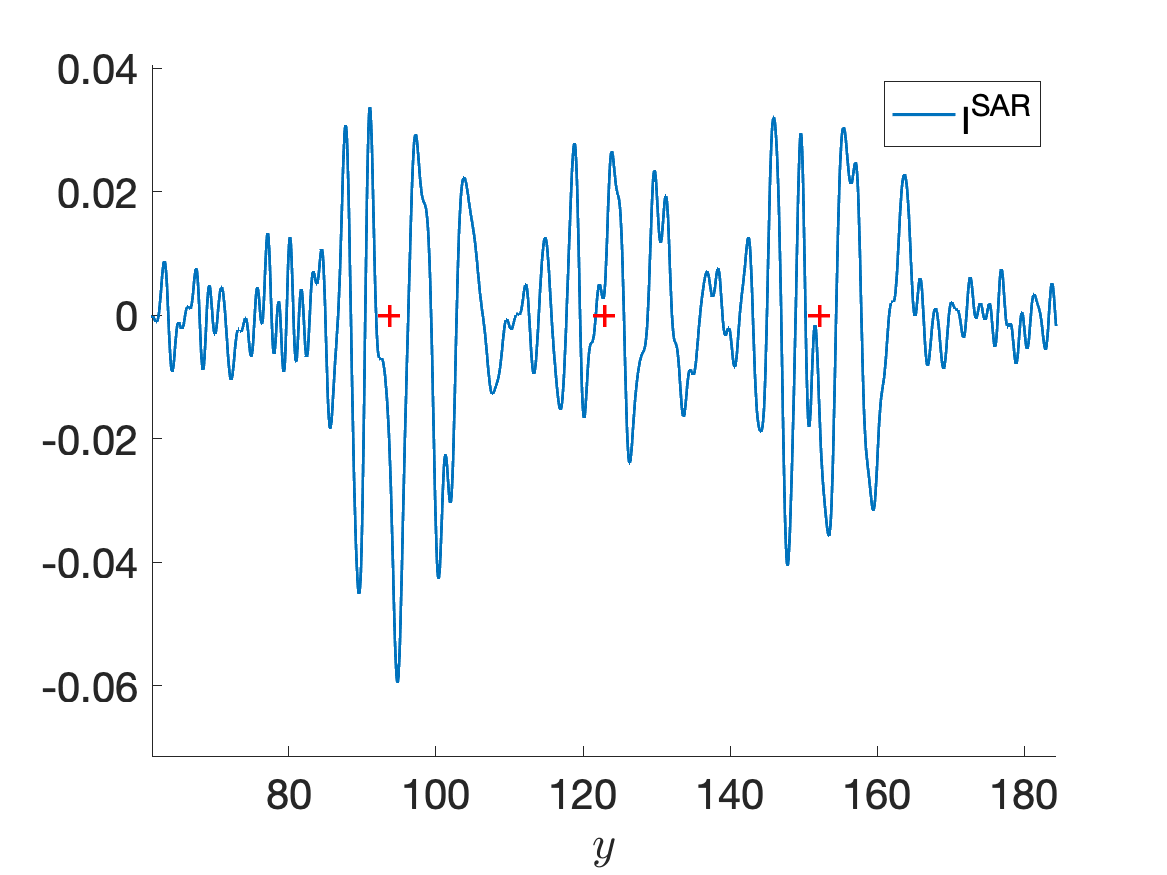
Note that in conventional SAR imaging there is no thresholding and the coefficient of variation of |SAR(y)|2superscriptsuperscriptSARy2\left|\mathcal{I}^{{\scalebox{0.5}[0.4]{SAR}}}({{\itbf y}})\right|^{2} is equal to one when there is no additive noise [5]. The numerical simulations in section 5 illustrate how the statistical instability of conventional SAR manifests: the images change dramatically with the realizations of the fluctuations μ𝜇\mu, they have large artifacts and thus cannot be used to estimate the support of the reflectivity.

For the additive noise contribution we give the covariance of the fluctuations

Cov[W(y,y),W(z,z)]Covsubscript𝑊ysuperscriptysubscript𝑊zsuperscriptz\displaystyle\mbox{Cov}\left[\mathcal{I}_{{}_{W}}({{\itbf y}},{{\itbf y}}^{\prime}),\mathcal{I}_{{}_{W}}({{\itbf z}},{{\itbf z}}^{\prime})\right] =CW2exp[(yz)2h2(yz)22h2+2iko(yz)]absentsuperscriptsubscript𝐶𝑊2superscriptsubscript𝑦parallel-tosubscript𝑧parallel-to2superscriptsubscriptparallel-to2superscript𝑦𝑧22superscript22𝑖subscript𝑘𝑜subscript𝑦parallel-tosubscript𝑧parallel-to\displaystyle=C_{{}_{W}}^{2}\exp\Big{[}-\frac{(y_{\parallel}-z_{\parallel})^{2}}{h_{\parallel}^{2}}-\frac{(y-z)^{2}}{2h^{2}}+2ik_{o}(y_{\parallel}-z_{\parallel})\Big{]}
×exp[(yz)2h2(yz)22h22iko(yz)],absentsuperscriptsuperscriptsubscript𝑦parallel-tosuperscriptsubscript𝑧parallel-to2superscriptsubscriptparallel-to2superscriptsuperscript𝑦superscript𝑧22superscript22𝑖subscript𝑘𝑜superscriptsubscript𝑦parallel-tosuperscriptsubscript𝑧parallel-to\displaystyle\times\exp\Big{[}-\frac{(y_{\parallel}^{\prime}-z_{\parallel}^{\prime})^{2}}{h_{\parallel}^{2}}-\frac{(y^{\prime}-z^{\prime})^{2}}{2h^{2}}-2ik_{o}(y_{\parallel}^{\prime}-z_{\parallel}^{\prime})\Big{]}, (34)

which simplifies for the CINT imaging function to

Cov[WCINT(y),WCINT(z)]CovsubscriptsuperscriptCINT𝑊ysubscriptsuperscriptCINT𝑊z\displaystyle\mbox{Cov}\left[\mathcal{I}^{\scalebox{0.5}[0.4]{CINT}}_{{}_{W}}({{\itbf y}}),\mathcal{I}^{\scalebox{0.5}[0.4]{CINT}}_{{}_{W}}({{\itbf z}})\right] =CW2exp[2(yz)2h2(yz)2h2].absentsuperscriptsubscript𝐶𝑊22superscriptsubscript𝑦parallel-tosubscript𝑧parallel-to2superscriptsubscriptparallel-to2superscript𝑦𝑧2superscript2\displaystyle=C_{{}_{W}}^{2}\exp\Big{[}-\frac{2(y_{\parallel}-z_{\parallel})^{2}}{h_{\parallel}^{2}}-\frac{(y-z)^{2}}{h^{2}}\Big{]}. (35)

Since |𝔼[W(y,y)]|2=O(CW2)superscript𝔼delimited-[]subscript𝑊ysuperscripty2𝑂superscriptsubscript𝐶𝑊2\left|\mathbb{E}\left[\mathcal{I}_{{}_{W}}({{\itbf y}},{{\itbf y}}^{\prime})\right]\right|^{2}=O(C_{{}_{W}}^{2}), the noise contribution to two-point or to regular CINT imaging is not statistically stable. It causes speckle with relative amplitude CW/C=O(σW2)subscript𝐶𝑊𝐶𝑂superscriptsubscript𝜎𝑊2C_{{}_{W}}/C=O(\sigma_{{}_{W}}^{2}) and with speckle size of order hh in cross range and hsubscriptparallel-toh_{\parallel} in range. Such speckle is not important for the CINT image, which has the poor resolution quantified by HH{\itbf{H}}. In fact, the speckle can be removed by using a low-pass filter on CINT(y)superscriptCINTy\mathcal{I}^{\scalebox{0.5}[0.4]{CINT}}({{\itbf y}}). However, noise affects the two-point CINT function (y,y)ysuperscripty\mathcal{I}({{\itbf y}},{{\itbf y}}^{\prime}), because the speckle size is similar to the resolution hh{\itbf{h}} of the offset vectors yyysuperscripty{{\itbf y}}-{{\itbf y}}^{\prime}. If the noise is weak (σW1much-less-thansubscript𝜎𝑊1\sigma_{{}_{W}}\ll 1), it can be viewed as a perturbation of the imaging methods described in [5] and in section 4, which predict the ideal resolution quantified by hh{\itbf{h}}. However, if σWsubscript𝜎𝑊\sigma_{{}_{W}} is larger, the speckle should be filtered out using a low-pass filter. We can still achieve a better resolution than with CINT, but not as good as the ideal one.

2.7 Generalization to other imaging setups

The imaging methods described in sections 34 are based on the expression (21), which gives the mean (20) of the two-point CINT function. We now describe how this expression generalizes to two other imaging setups:

\bullet Imaging sources with a passive array. Suppose that we had a collection of N+1𝑁1N+1 receivers at closely spaced locations (xj)j=0Nsuperscriptsubscriptsubscriptx𝑗𝑗0𝑁\big{(}{{\itbf x}}_{j}\big{)}_{j=0}^{N} in a line segment of length a𝑎a. Such a collection is called a passive array with aperture a𝑎a. The imaging problem would then be to localize a group of sources in the domain 𝒟𝒟\mathcal{D}, which gives a source term in the wave equation of the form S(x,t)𝑆x𝑡S({{\itbf x}},t) that generates a wave u(x,t)𝑢x𝑡u({{\itbf x}},t). This wave propagates through the random medium and it is received at the array. The data model

Rn(t)::subscript𝑅𝑛𝑡absent\displaystyle R_{n}(t): =u(xn,t)+Wn(t),absent𝑢subscriptx𝑛𝑡subscript𝑊𝑛𝑡\displaystyle={u({{\itbf x}}_{n},t)}+W_{n}(t),

with

u(xn,t)𝑢subscriptx𝑛𝑡\displaystyle{u({{\itbf x}}_{n},t)} =dω2πeiωt𝒟𝑑zS^(z,ω)G^μ(z,xn,ω),absentsubscript𝑑𝜔2𝜋superscript𝑒𝑖𝜔𝑡subscript𝒟differential-dz^𝑆z𝜔subscript^𝐺𝜇zsubscriptx𝑛𝜔\displaystyle=\int_{\mathbb{R}}\frac{d{\omega}}{2\pi}e^{-i{\omega}t}\int_{\mathcal{D}}d{{\itbf z}}\,\widehat{S}({{\itbf z}},{\omega})\widehat{G}_{\mu}({{\itbf z}},{{\itbf x}}_{n},{\omega}),

is very similar to (9), except for the one way propagation between the sources and the receivers, which is why in the equation above we have G^μsubscript^𝐺𝜇\widehat{G}_{\mu} and not G^μ2superscriptsubscript^𝐺𝜇2\widehat{G}_{\mu}^{2}. The two-point CINT function (y,y)ysuperscripty\mathcal{I}({{\itbf y}},{{\itbf y}}^{\prime}) is given by the same data processing as in (18), with

F^n(y,ω)=s^(ω)G^o(y,xn,ω)exp(xn2a2),subscript^𝐹𝑛y𝜔^𝑠𝜔subscript^𝐺𝑜ysubscriptx𝑛𝜔superscriptsubscript𝑥𝑛2superscript𝑎2\widehat{F}_{n}({{\itbf y}},\omega)=\widehat{s}({\omega})\widehat{G}_{o}({{\itbf y}},{{\itbf x}}_{n},{\omega})\exp\Big{(}-\frac{x_{n}^{2}}{a^{2}}\Big{)},

and s^(ω)=exp[(ωωo)2/(2B2)]^𝑠𝜔superscript𝜔subscript𝜔𝑜22superscript𝐵2\widehat{s}({\omega})=\exp[-({\omega}-{\omega}_{o})^{2}/(2B^{2})] a frequency filter, with Bωomuch-less-than𝐵subscript𝜔𝑜B\ll{\omega}_{o}. The expression of the expectation of (y,y)ysuperscripty\mathcal{I}({{\itbf y}},{{\itbf y}}^{\prime}) is (20) modified as follows: ρ(z)𝜌z\rho({{\itbf z}}) is replaced by S^(z,ωo)^𝑆zsubscript𝜔𝑜\widehat{S}({{\itbf z}},{\omega}_{o}) (assuming S^(z,ω)^𝑆z𝜔\widehat{S}({{\itbf z}},{\omega}) is almost constant over the frequency interval centered at ωosubscript𝜔𝑜{\omega}_{o} and bandwidth B𝐵B), and all the resolution parameters in (26)–(27) are divided by two.

\bullet Imaging with an active array. If we wished to image the reflectivity ρ𝜌\rho using an active array of sensors at xnsubscriptx𝑛{{\itbf x}}_{n}, for n=0,,N𝑛0𝑁n=0,\ldots,N, with linear aperture of length a𝑎a, the data would be collected as follows: The array would emit a probing signal f(t)=s(t)+c.c.formulae-sequence𝑓𝑡𝑠𝑡𝑐𝑐f(t)=s(t)+c.c. from one sensor location xnsubscriptx𝑛{{\itbf x}}_{n} at a time, and the response

Rn,n(t)=ureal(xn,t;xn)+Wn,n(t),subscript𝑅superscript𝑛𝑛𝑡subscript𝑢realsubscriptxsuperscript𝑛𝑡subscriptx𝑛subscript𝑊superscript𝑛𝑛𝑡R_{n^{\prime},n}(t)=u_{{\rm real}}({{\itbf x}}_{n^{\prime}},t;{{\itbf x}}_{n})+W_{n^{\prime},n}(t),

with

ureal(xn,t;xn)=dω2πeiωts^(ω)k2(ω)𝒟𝑑zρ(z)G^μ(z,xn,ω)G^μ(z,xn,ω)+c.c.formulae-sequencesubscript𝑢realsubscriptxsuperscript𝑛𝑡subscriptx𝑛subscript𝑑𝜔2𝜋superscript𝑒𝑖𝜔𝑡^𝑠𝜔superscript𝑘2𝜔subscript𝒟differential-dz𝜌zsubscript^𝐺𝜇zsubscriptx𝑛𝜔subscript^𝐺𝜇zsubscriptxsuperscript𝑛𝜔𝑐𝑐u_{{\rm real}}({{\itbf x}}_{n^{\prime}},t;{{\itbf x}}_{n})=\int_{\mathbb{R}}\frac{d{\omega}}{2\pi}e^{-i{\omega}t}\widehat{s}({\omega})k^{2}({\omega})\int_{\mathcal{D}}d{{\itbf z}}\,\rho({{\itbf z}})\widehat{G}_{\mu}({{\itbf z}},{{\itbf x}}_{n},{\omega})\widehat{G}_{\mu}({{\itbf z}},{{\itbf x}}_{n^{\prime}},{\omega})+c.c.

would be measured at all the sensor locations xnsubscriptxsuperscript𝑛{{\itbf x}}_{n^{\prime}}, for n=0,,Nsuperscript𝑛0𝑁n^{\prime}=0,\ldots,N, where Wn,n(t)subscript𝑊superscript𝑛𝑛𝑡W_{n^{\prime},n}(t) is the additive noise. Here we used again the Born approximation. The calculation of the two-point CINT function (y,y)ysuperscripty\mathcal{I}({{\itbf y}},{{\itbf y}}^{\prime}) from the response matrix (Rn,n(t))n,n=0Nsuperscriptsubscriptsubscript𝑅superscript𝑛𝑛𝑡𝑛superscript𝑛0𝑁\big{(}R_{n^{\prime},n}(t)\big{)}_{n,n^{\prime}=0}^{N} is like in (18), with the following differences: The matching is done for each source-receiver pair, using the field

F^n,n(y,ω)=s^(ω)G^o(y,xn,ω)G^o(y,xn,ω)exp(xn2+xn2a2),subscript^𝐹superscript𝑛𝑛y𝜔^𝑠𝜔subscript^𝐺𝑜ysubscriptx𝑛𝜔subscript^𝐺𝑜ysubscriptxsuperscript𝑛𝜔superscriptsubscript𝑥𝑛2superscriptsubscript𝑥superscript𝑛2superscript𝑎2\displaystyle\widehat{F}_{n^{\prime},n}({{\itbf y}},{\omega})=\widehat{s}({\omega})\widehat{G}_{o}({{\itbf y}},{{\itbf x}}_{n},{\omega})\widehat{G}_{o}({{\itbf y}},{{\itbf x}}_{n^{\prime}},{\omega})\exp\Big{(}-\frac{x_{n}^{2}+x_{n^{\prime}}^{2}}{a^{2}}\Big{)},

and the sensor offset thresholding is done for both the source and receiver pairs. We refer to [10, 7] for the study of the CINT imaging function CINT(y)=(y,y)superscriptCINTyyy\mathcal{I}^{{\scalebox{0.5}[0.4]{CINT}}}({{\itbf y}})=\mathcal{I}({{\itbf y}},{{\itbf y}}) in this setup. Using the expressions of the statistical moments of the Green’s function, it follows after some calculation that the expression of 𝔼[(y,y)]𝔼delimited-[]ysuperscripty\mathbb{E}[\mathcal{I}({{\itbf y}},{{\itbf y}}^{\prime})] is like that in (20) and the statistical stability is ensured provided that the condition 𝒳𝒳dless-than-or-similar-to𝒳subscript𝒳𝑑\mathcal{X}\lesssim\mathcal{X}_{d}, ΩΩdless-than-or-similar-toΩsubscriptΩ𝑑\Omega\lesssim\Omega_{d} is satisfied.

3 Spectral approach to imaging

In this section we study the linear integral operator \mathcal{L} with kernel given by the two-point CINT function (18), and show that its leading eigenfunction can be used to image the reflectivity of a group of point-like reflectors. For simplicity, the imaging is carried out in a range-bin i.e., it is one-dimensional, in the cross-range direction. However, it is possible to extend the imaging to the range and cross-range plane, as explained briefly at the end of the section. We assume that the threshold parameters are chosen as explained in section 2.6, so we can approximate (y,y)ysuperscripty\mathcal{I}({{\itbf y}},{{\itbf y}}^{\prime}) by its expectation. The additive noise is ignored in the spectral analysis of \mathcal{L}, although it could be taken into account using the tools in [25]. Nevertheless, the numerical simulations in section 5 are for noisy data.

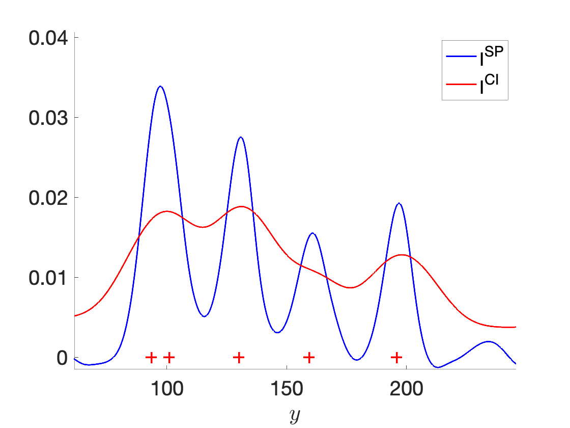
Before we begin, let us explain how our approach differs from other imaging methods that use spectral analysis. The popular MUSIC (Multiple Signal Classification) method, which is related to linear sampling [13] and also the factorization method [26], uses the spectral decomposition of the response matrix at a single frequency, collected by an active array of sensors to locate small reflectors [30, 2]. It can be modified to handle strong additive noise as shown in [4], but it does not work in random media, where cross correlations have emerged as an important tool for mitigating the wave distortion. In [28, 29] cross correlations are used to calculate a two-point function like (18), but since the imaging is through a homogeneous medium, there is no thresholding. Therefore, the two-point function is an outer product, like (29), and its samples on the search grid define a rank-one matrix whose leading eigenvector can be used to image. Due to the thresholding needed for statistical stability of imaging in random media, our two-point CINT function is not an outer product and the spectral analysis is much more complicated. It reveals that the leading eigenfunction is useful for improving the resolution of imaging only under a sufficient separation condition between the reflectors. Furthermore, the resolution of the resulting image is surprising: It is of the order Hh𝐻\sqrt{Hh}, which is better than the CINT resolution H𝐻H but worse than the ideal resolution hh.

3.1 The integral operator and the imaging function

Consider a reflectivity of the form

ρ(z)=j=1Mρjδ(zzj),𝜌zsuperscriptsubscript𝑗1𝑀subscript𝜌𝑗𝛿zsubscriptz𝑗\rho({{\itbf z}})=\sum_{j=1}^{M}\rho_{j}\delta({{\itbf z}}-{{\itbf z}}_{j}), (36)

which models a group of M𝑀M point-like reflectors at zjsubscriptz𝑗{{\itbf z}}_{j}, with reflectivity ρjsubscript𝜌𝑗\rho_{j}\in\mathbb{R}, for j=1,,M𝑗1𝑀j=1,\ldots,M. Because we image in a fixed range bin 𝒟zsubscript𝒟subscript𝑧parallel-to\mathcal{D}_{z_{\parallel}} at range coordinate zsubscript𝑧parallel-toz_{\parallel}, we assume that the reflector locations are zj=(zj,z)subscriptz𝑗subscript𝑧𝑗subscript𝑧parallel-to{{\itbf z}}_{j}=(z_{j},z_{\parallel}) and the search points in 𝒟zsubscript𝒟subscript𝑧parallel-to\mathcal{D}_{z_{\parallel}} are y=(y,z)y𝑦subscript𝑧parallel-to{{\itbf y}}=(y,z_{\parallel}) and y=(y,z)superscriptysuperscript𝑦subscript𝑧parallel-to{{\itbf y}}^{\prime}=(y^{\prime},z_{\parallel}).

The proposed spectral based imaging function is

SP(y=(y,z)):=V0(y),assignsuperscriptSPy𝑦subscript𝑧parallel-tosuperscriptsubscript𝑉0𝑦\mathcal{I}^{{\scalebox{0.5}[0.4]{SP}}}({{\itbf y}}=(y,z_{\parallel})):=V_{0}^{\mathcal{I}}(y), (37)

where V0(y)superscriptsubscript𝑉0𝑦V_{0}^{\mathcal{I}}(y) is the leading eigenfunction of the integral operator superscript{\cal L}^{\cal I} with kernel (y=(y,z),y=(y,z))formulae-sequencey𝑦subscript𝑧parallel-tosuperscriptysuperscript𝑦subscript𝑧parallel-to{\cal I}({{\itbf y}}=(y,z_{\parallel}),{{\itbf y}}^{\prime}=(y^{\prime},z_{\parallel})):

:L2()L2(),φ(y)=𝑑y((y,z),(y,z))φ(y),φL2().:superscriptformulae-sequencemaps-tosuperscript𝐿2superscript𝐿2formulae-sequencesuperscript𝜑𝑦subscriptdifferential-dsuperscript𝑦𝑦subscript𝑧parallel-tosuperscript𝑦subscript𝑧parallel-to𝜑superscript𝑦for-all𝜑superscript𝐿2\mathcal{L}^{\mathcal{I}}:L^{2}(\mathbb{R})\mapsto L^{2}(\mathbb{R}),\qquad\mathcal{L}^{\mathcal{I}}\varphi(y)=\int_{\mathbb{R}}dy^{\prime}\,{\cal I}((y,z_{\parallel}),(y^{\prime},z_{\parallel}))\varphi(y^{\prime}),\qquad\forall\,\varphi\in L^{2}(\mathbb{R}).

This kernel is Hermitian and square integrable, so superscript\mathcal{L}^{\mathcal{I}} is self-adjoint and Hilbert-Schmidt [11, Chapter 6]. We also show in Appendix C.1 that it is positive semidefinite. Our goal in the remainder of the section is to explain when and how the imaging function SPsuperscriptSP\mathcal{I}^{{\scalebox{0.5}[0.4]{SP}}} works.

Substituting (36) into the expression of the expectation of the two-point CINT function obtained from (20)–(21) and using the statistical stability (y,y)𝔼[(y,y)]ysuperscripty𝔼delimited-[]ysuperscripty\mathcal{I}({{\itbf y}},{{\itbf y}}^{\prime})\approx\mathbb{E}\big{[}\mathcal{I}({{\itbf y}},{{\itbf y}}^{\prime})\big{]}, we get

(y,y)𝕂(y,y),ysuperscripty𝕂𝑦superscript𝑦\mathcal{I}({{\itbf y}},{{\itbf y}}^{\prime})\approx\mathbb{K}(y,y^{\prime}),

with

𝕂(y,y)𝕂𝑦superscript𝑦\displaystyle\mathbb{K}(y,y^{\prime}) :=Cj,j=1MρjρjKH(zj+zj2y+y2)Kh((zjzj)(yy)),assignabsent𝐶superscriptsubscript𝑗superscript𝑗1𝑀subscript𝜌𝑗subscript𝜌superscript𝑗subscript𝐾𝐻subscript𝑧𝑗subscript𝑧superscript𝑗2𝑦superscript𝑦2subscript𝐾subscript𝑧𝑗subscript𝑧superscript𝑗𝑦superscript𝑦\displaystyle:=C\sum_{j,j^{\prime}=1}^{M}\rho_{j}\rho_{j^{\prime}}K_{H}\Big{(}\frac{z_{j}+z_{j^{\prime}}}{2}-\frac{y+y^{\prime}}{2}\Big{)}K_{h}\big{(}(z_{j}-z_{j^{\prime}})-(y-y^{\prime})\big{)}, (38)

where KHsubscript𝐾𝐻K_{H} and Khsubscript𝐾K_{h} are defined as in (25), H𝐻H and hh are given in (26)–(27), and C𝐶C is the redefined constant equal to what we had in (21), divided by 2πHh2𝜋subscript𝐻parallel-tosubscriptparallel-to2\pi H_{\parallel}h_{\parallel}. The linear integral operator that we wish to study is

:L2()L2(),φ(y)=𝑑y𝕂(y,y)φ(y),φL2().:formulae-sequencemaps-tosuperscript𝐿2superscript𝐿2formulae-sequence𝜑𝑦subscriptdifferential-dsuperscript𝑦𝕂𝑦superscript𝑦𝜑superscript𝑦for-all𝜑superscript𝐿2\mathcal{L}:L^{2}(\mathbb{R})\mapsto L^{2}(\mathbb{R}),\qquad\mathcal{L}\varphi(y)=\int_{\mathbb{R}}dy^{\prime}\,\mathbb{K}(y,y^{\prime})\varphi(y^{\prime}),\qquad\forall\,\varphi\in L^{2}(\mathbb{R}). (39)

Again it can be verified that \mathcal{L} is self-adjoint, Hilbert-Schmidt, and positive semidefinite. The spectral theorem [11, Chapter 6] then gives that the eigenfunctions (Vn(y))n0subscriptsubscript𝑉𝑛𝑦𝑛0\left(V_{n}(y)\right)_{n\geq 0} of \mathcal{L} form an orthonormal basis of L2()superscript𝐿2L^{2}(\mathbb{R}) and the eigenvalues (Λn)n0subscriptsubscriptΛ𝑛𝑛0\left(\Lambda_{n}\right)_{n\geq 0} are non-negative. These eigenvalues are sorted in decreasing order and limnΛn=0subscript𝑛subscriptΛ𝑛0\lim_{n\to\infty}\Lambda_{n}=0.

3.2 The spectral decomposition

It is instructive to consider first the case of a single reflector, modeled by the reflectivity ρ(z)=ρjδ(zzj)𝜌zsubscript𝜌𝑗𝛿zsubscriptz𝑗\rho({{\itbf z}})=\rho_{j}\delta({{\itbf z}}-{{\itbf z}}_{j}), for any given j=1,,M𝑗1𝑀j=1,\ldots,M. The operator (39) simplifies for such a reflectivity to

j:L2()L2(),jφ(y)=𝑑y𝕂j(y,y)φ(y),φL2(),:subscript𝑗formulae-sequencemaps-tosuperscript𝐿2superscript𝐿2formulae-sequencesubscript𝑗𝜑𝑦subscriptdifferential-dsuperscript𝑦subscript𝕂𝑗𝑦superscript𝑦𝜑superscript𝑦for-all𝜑superscript𝐿2\mathcal{L}_{j}:L^{2}(\mathbb{R})\mapsto L^{2}(\mathbb{R}),\qquad\mathcal{L}_{j}\varphi(y)=\int_{\mathbb{R}}dy^{\prime}\,\mathbb{K}_{j}(y,y^{\prime})\varphi(y^{\prime}),\qquad\forall\,\varphi\in L^{2}(\mathbb{R}), (40)

with

𝕂j(y,y):=Cρj2KH(zjy+y2)Kh(yy).assignsubscript𝕂𝑗𝑦superscript𝑦𝐶superscriptsubscript𝜌𝑗2subscript𝐾𝐻subscript𝑧𝑗𝑦superscript𝑦2subscript𝐾superscript𝑦𝑦\mathbb{K}_{j}(y,y^{\prime}):=C\rho_{j}^{2}K_{H}\Big{(}z_{j}-\frac{y+y^{\prime}}{2}\Big{)}K_{h}(y^{\prime}-y). (41)

Because the kernel (41) is non-negative, jsubscript𝑗\mathcal{L}_{j} is a positive operator with non-negative leading eigenfunction, by the Krein-Rutman theorem [27]. For imaging a single reflector we only need this eigenfunction, but the result for the reflectivity (36) uses the full spectral decomposition of jsubscript𝑗\mathcal{L}_{j}, given in the next proposition proved in Appendix C.2.

Proposition 1.

Let j𝑗j be any index in the set {1,,M}1𝑀\{1,\ldots,M\}. The eigenvalues of the operator jsubscript𝑗\mathcal{L}_{j} are

Λj,n=Cρj22π(H+h/2)(Hh/2H+h/2)n,n0,formulae-sequencesubscriptΛ𝑗𝑛𝐶superscriptsubscript𝜌𝑗22𝜋𝐻2superscript𝐻2𝐻2𝑛𝑛0\Lambda_{j,n}=\frac{C\rho_{j}^{2}}{\sqrt{2\pi}(H+h/2)}\left(\frac{H-h/2}{H+h/2}\right)^{n},\qquad n\geq 0, (42)

and the eigenfunctions are given by

Vj,n(y)=Cj,nexp[(yzj)22Hh]pn(yzjHh),n0,formulae-sequencesubscript𝑉𝑗𝑛𝑦subscript𝐶𝑗𝑛superscript𝑦subscript𝑧𝑗22𝐻subscript𝑝𝑛𝑦subscript𝑧𝑗𝐻𝑛0V_{j,n}(y)=C_{j,n}\exp\Big{[}-\frac{(y-z_{j})^{2}}{2Hh}\Big{]}p_{n}\Big{(}\frac{y-z_{j}}{\sqrt{Hh}}\Big{)},\qquad n\geq 0, (43)

for polynomials pn(ξ)subscript𝑝𝑛𝜉p_{n}(\xi) of degree n𝑛n,

pn(ξ)=ξn+l=0n1γnlξl,subscript𝑝𝑛𝜉superscript𝜉𝑛superscriptsubscript𝑙0𝑛1subscript𝛾𝑛𝑙superscript𝜉𝑙p_{n}(\xi)=\xi^{n}+\sum_{l=0}^{n-1}\gamma_{nl}\xi^{l}, (44)

with p0(ξ)=1subscript𝑝0𝜉1p_{0}(\xi)=1 and with coefficients γnlsubscript𝛾𝑛𝑙\gamma_{nl} given explicitly in Appendix C.2. Here Cj,nsubscript𝐶𝑗𝑛C_{j,n} is a normalizing constant so that Vj,nL2()=1subscriptnormsubscript𝑉𝑗𝑛superscript𝐿21\|V_{j,n}\|_{L^{2}(\mathbb{R})}=1.

We conclude from (43) that the leading eigenfunction

Vj,0(y)=12πHhexp[(yzj)22Hh],subscript𝑉𝑗0𝑦12𝜋𝐻superscript𝑦subscript𝑧𝑗22𝐻V_{j,0}(y)=\frac{1}{\sqrt{2\pi Hh}}\exp\Big{[}-\frac{(y-z_{j})^{2}}{2Hh}\Big{]}, (45)

peaks at the location zjsubscript𝑧𝑗z_{j} of the reflector, and it is large for |yzj|=O(Hh)𝑦subscript𝑧𝑗𝑂𝐻|y-z_{j}|=O(\sqrt{Hh}). Thus, this eigenfunction gives an imaging function for a scene with a single reflector, with resolution Hh𝐻\sqrt{Hh} that is much better than the CINT resolution H𝐻H, but not as good as the ideal resolution hh.

Now we can state the result for the reflectivity (36), which models M𝑀M point-like reflectors. If these reflectors are not sufficiently spaced out, then the image (37) peaks near their locations, but it does not have better resolution than CINT, as shown with numerical simulations in section 5. The separation condition that allows a better localization with V0(y)subscript𝑉0𝑦V_{0}(y) is

ζ:=min1j,lM,jl|zjzl|3H>1.assign𝜁subscriptformulae-sequence1𝑗formulae-sequence𝑙𝑀𝑗𝑙subscript𝑧𝑗subscript𝑧𝑙3𝐻1\zeta:=\min_{1\leq j,l\leq M,j\neq l}\frac{|z_{j}-z_{l}|}{3H}>1. (46)

The next proposition proved in Appendix C.3 states that if (46) holds, then the interaction between the reflectors is weak and the spectral decomposition of \mathcal{L} is determined by the decomposition of the operators jsubscript𝑗\mathcal{L}_{j}, given in Proposition 1.

Proposition 2.

If the point-like reflectors are well separated, as stated in (46), then the spectral decomposition of the operator \mathcal{L} defined in (39) is as follows: The eigenvalues are

Λn=j=1MΛj,n+O(e9ζ2/2),n0,formulae-sequencesubscriptΛ𝑛superscriptsubscript𝑗1𝑀subscriptΛ𝑗𝑛𝑂superscript𝑒9superscript𝜁22𝑛0\Lambda_{n}=\sum_{j=1}^{M}\Lambda_{j,n}+O\left(e^{-9\zeta^{2}/2}\right),\qquad n\geq 0, (47)

with terms given in (42) and the eigenfunctions are approximated by the sum

Vn(y)=Cnj=1MρjVj,n(y)+O(e9ζ2/2),n0,formulae-sequencesubscript𝑉𝑛𝑦subscript𝐶𝑛superscriptsubscript𝑗1𝑀subscript𝜌𝑗subscript𝑉𝑗𝑛𝑦𝑂superscript𝑒9superscript𝜁22𝑛0V_{n}(y)=C_{n}\sum_{j=1}^{M}\rho_{j}V_{j,n}(y)+O\left(e^{-9\zeta^{2}/2}\right),\qquad n\geq 0, (48)

with terms given in (43). Here Cnsubscript𝐶𝑛C_{n} is a normalizing constant so that VnL2()=1subscriptnormsubscript𝑉𝑛superscript𝐿21\|V_{n}\|_{L^{2}(\mathbb{R})}=1.

3.3 Discussion

It may seem peculiar that according to Propositions 1 and 2, the imaging function

SP(y,z)=V0(y)V0(y)C0j=1Mρjexp[(yzj)22Hh]superscriptSP𝑦subscript𝑧parallel-tosuperscriptsubscript𝑉0𝑦subscript𝑉0𝑦subscript𝐶0superscriptsubscript𝑗1𝑀subscript𝜌𝑗superscript𝑦subscript𝑧𝑗22𝐻\mathcal{I}^{{\scalebox{0.5}[0.4]{SP}}}(y,z_{\parallel})=V_{0}^{\mathcal{I}}(y)\approx V_{0}(y)\approx C_{0}\sum_{j=1}^{M}\rho_{j}\exp\left[-\frac{(y-z_{j})^{2}}{2Hh}\right] (49)

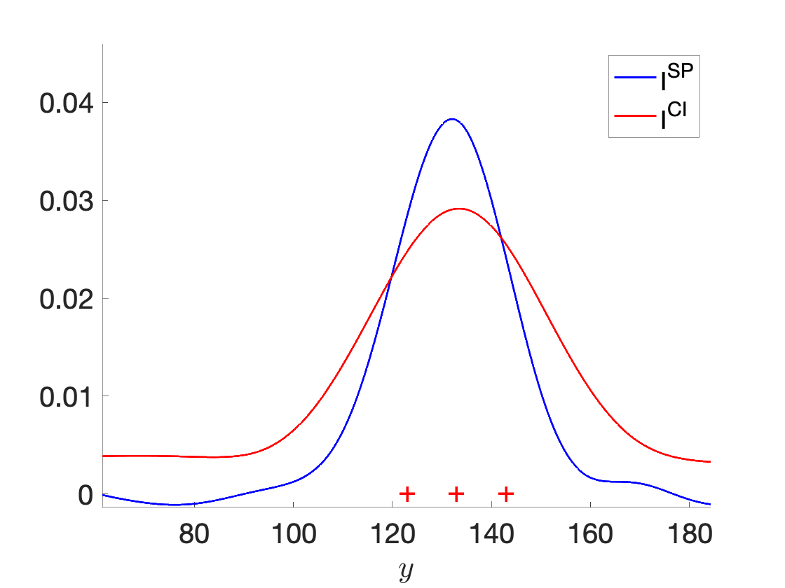
has resolution Hh𝐻\sqrt{Hh} and yet it assumes the larger separation condition (46). The numerical simulations in section 5 show that (46) can be improved a bit to ζ1/3greater-than-or-equivalent-to𝜁13\zeta\gtrsim 1/3. Still, the needed separation is of the order of the resolution of CINT, so what do we gain when imaging with SP(y)superscriptSP𝑦\mathcal{I}^{{\scalebox{0.5}[0.4]{SP}}}(y)? There are two clear advantages:

1. The localization of the reflectors with (37) is more precise than with CINT and does not require deconvolution as in [8]. Therefore, (37) is more robust to random fluctuations of the two-point CINT function about its mean and also to additive noise.

2. The CINT imaging approach cannot distinguish between positive and negative reflectivities. This can be seen from the expression (38) evaluated on the diagonal

CINT(y=(y,z))superscriptCINTy𝑦subscript𝑧parallel-to\displaystyle\mathcal{I}^{\scalebox{0.5}[0.4]{CINT}}({{\itbf y}}=(y,z_{\parallel})) =(y,y)absentyy\displaystyle=\mathcal{I}({{\itbf y}},{{\itbf y}})
Cj,j=1Mρjρj𝒦H(zj+zj2y)𝒦h(zjzj),absent𝐶superscriptsubscript𝑗superscript𝑗1𝑀subscript𝜌𝑗subscript𝜌superscript𝑗subscript𝒦𝐻subscript𝑧𝑗subscript𝑧superscript𝑗2𝑦subscript𝒦subscript𝑧𝑗subscript𝑧superscript𝑗\displaystyle\approx C\sum_{j,j^{\prime}=1}^{M}\rho_{j}\rho_{j^{\prime}}\mathcal{K}_{H}\Big{(}\frac{z_{j}+z_{j^{\prime}}}{2}-y\Big{)}\mathcal{K}_{h}(z_{j}-z_{j^{\prime}}), (50)

which simplifies under the assumption (46) to

CINT(y)C2πhHj=1Mρj2exp[(yzj)22H2].superscriptCINTy𝐶2𝜋𝐻superscriptsubscript𝑗1𝑀superscriptsubscript𝜌𝑗2superscript𝑦subscript𝑧𝑗22superscript𝐻2\displaystyle\mathcal{I}^{\scalebox{0.5}[0.4]{CINT}}({{\itbf y}})\approx\frac{C}{2\pi hH}\sum_{j=1}^{M}\rho_{j}^{2}\exp\Big{[}-\frac{(y-z_{j})^{2}}{2H^{2}}\Big{]}. (51)

Compare this with (49), which in addition to better localization of the reflectors, it distinguishes the sign of their reflectivity.

We end with the remark that although we considered imaging at fixed range zsubscript𝑧parallel-toz_{\parallel}, the spectral approach can be extended to imaging in range and cross range. This extension is needed even for a fixed range bin 𝒟zsubscript𝒟subscript𝑧parallel-to\mathcal{D}_{z_{\parallel}}, because arrival times can be estimated up to O(1/Ω)𝑂1ΩO(1/\Omega) precision, and thus the points yy{{\itbf y}} in 𝒟zsubscript𝒟subscript𝑧parallel-to\mathcal{D}_{z_{\parallel}} are at coordinates y=(y,z+O(H))y𝑦subscript𝑧parallel-to𝑂subscript𝐻parallel-to{{\itbf y}}=\big{(}y,z_{\parallel}+O(H_{\parallel})\big{)}. Indeed, for the reflectivity (36), the kernel of the integral operator \mathcal{L} is

(y,y)e2iko(yy)(20)𝒥(y,y)=(21)Cj,j=1Mρko(zj)ρko(zj)¯superscriptitalic-(20italic-)ysuperscriptysuperscript𝑒2𝑖subscript𝑘𝑜subscript𝑦parallel-tosuperscriptsubscript𝑦parallel-to𝒥ysuperscriptysuperscriptitalic-(21italic-)𝐶superscriptsubscript𝑗superscript𝑗1𝑀subscript𝜌subscript𝑘𝑜subscriptz𝑗¯subscript𝜌subscript𝑘𝑜subscriptzsuperscript𝑗\displaystyle\mathcal{I}({{\itbf y}},{{\itbf y}}^{\prime})e^{2ik_{o}(y_{\parallel}-y_{\parallel}^{\prime})}\stackrel{{\scriptstyle\eqref{eq:2.1}}}{{\approx}}\mathcal{J}({{\itbf y}},{{\itbf y}}^{\prime})\stackrel{{\scriptstyle\eqref{eq:2.2}}}{{=}}C\sum_{j,j^{\prime}=1}^{M}\rho_{k_{o}}({{\itbf z}}_{j})\overline{\rho_{k_{o}}({{\itbf z}}_{j^{\prime}})}
×𝒦H(zj+zj2y+y2)𝒦h((zjzj)(yy)),absentsubscript𝒦Hsubscriptz𝑗subscriptzsuperscript𝑗2ysuperscripty2subscript𝒦hsubscriptz𝑗subscriptzsuperscript𝑗ysuperscripty\displaystyle\times\mathcal{K}_{{\itbf{H}}}\Big{(}\frac{{{\itbf z}}_{j}+{{\itbf z}}_{j^{\prime}}}{2}-\frac{{{\itbf y}}+{{\itbf y}}^{\prime}}{2}\Big{)}\mathcal{K}_{{\itbf{h}}}\big{(}({{\itbf z}}_{j}-{{\itbf z}}_{j^{\prime}})-({{\itbf y}}-{{\itbf y}}^{\prime})\big{)},

with ρko(zj)=ρjexp(2ikoz,j),\rho_{k_{o}}({{\itbf z}}_{j})=\rho_{j}\exp(-2ik_{o}z_{\parallel,j}), for j=1,,M.𝑗1𝑀j=1,\ldots,M. It is easily verified that this \mathcal{L} is also self-adjoint, positive semidefinite and Hilbert-Schmidt. Moreover, the operator jsubscript𝑗\mathcal{L}_{j} associated to a single reflector at zjsubscriptz𝑗{{\itbf z}}_{j} has a separable kernel in range and cross range

𝒥j(y,y)=Cρj2𝒦H(zjy+y2)𝒦h(yy),subscript𝒥𝑗ysuperscripty𝐶superscriptsubscript𝜌𝑗2subscript𝒦Hsubscriptz𝑗ysuperscripty2subscript𝒦hysuperscripty\mathcal{J}_{j}({{\itbf y}},{{\itbf y}}^{\prime})=C\rho_{j}^{2}\mathcal{K}_{{\itbf{H}}}\Big{(}{{\itbf z}}_{j}-\frac{{{\itbf y}}+{{\itbf y}}^{\prime}}{2}\Big{)}\mathcal{K}_{{\itbf{h}}}({{\itbf y}}-{{\itbf y}}^{\prime}),

so its spectral analysis can be carried out in the two coordinates as we have done in this section. Then, under a sufficient separation condition between the reflectors, the spectrum of the operator with kernel 𝒥(y,y)𝒥ysuperscripty\mathcal{J}({{\itbf y}},{{\itbf y}}^{\prime}) can be written in terms of the spectra of the operators jsubscript𝑗\mathcal{L}_{j}, similar to Proposition 2.

4 Optimization approach to imaging

In this section we describe the second approach for obtaining an image from the two-point CINT function (18). It works for a general reflectivity ρ(y)𝜌y\rho({{\itbf y}}) of compact support, not just for point reflectors, as long as |ρ(y)|𝜌y|\rho({{\itbf y}})| is small enough so that the Born approximation data model (9) is adequate.

Like in the previous section, we assume that (y,y)ysuperscripty\mathcal{I}({{\itbf y}},{{\itbf y}}^{\prime}) is computed using proper thresholding, so we can approximate it in the noiseless case by its expectation given in (20)–(21)

(y,y)Ce2iko(yy)𝒟𝑑z𝒟𝑑zρko(z)ρko(z)¯𝒦H(z+z2y+y2)ysuperscripty𝐶superscript𝑒2𝑖subscript𝑘𝑜subscript𝑦parallel-tosuperscriptsubscript𝑦parallel-tosubscript𝒟differential-dzsubscript𝒟differential-dsuperscriptzsubscript𝜌subscript𝑘𝑜z¯subscript𝜌subscript𝑘𝑜superscriptzsubscript𝒦Hzsuperscriptz2ysuperscripty2\displaystyle\mathcal{I}({{\itbf y}},{{\itbf y}}^{\prime})\approx Ce^{-2ik_{o}(y_{\parallel}-y_{\parallel}^{\prime})}\int_{\mathcal{D}}d{{\itbf z}}\int_{\mathcal{D}}d{{\itbf z}}^{\prime}\rho_{k_{o}}({{\itbf z}})\overline{\rho_{k_{o}}({{\itbf z}}^{\prime})}\mathcal{K}_{{\itbf{H}}}\left(\frac{{{\itbf z}}+{{\itbf z}}^{\prime}}{2}-\frac{{{\itbf y}}+{{\itbf y}}^{\prime}}{2}\right)
×𝒦h((zz)(yy)),absentsubscript𝒦hzsuperscriptzysuperscripty\displaystyle\times\mathcal{K}_{{\itbf{h}}}\left(({{\itbf z}}-{{\itbf z}}^{\prime})-({{\itbf y}}-{{\itbf y}}^{\prime})\right), (52)

where ρko(z)subscript𝜌subscript𝑘𝑜z\rho_{k_{o}}({{\itbf z}}) is the modulated reflectivity defined in (23). The noise adds speckle to the image, as explained in section 2.6, and we comment at the end of the section how it can be mitigated, at the expense of resolution.

4.1 The case of noiseless data

Let us multiply (52) by exp[2iko(yy)]2𝑖subscript𝑘𝑜subscript𝑦parallel-tosuperscriptsubscript𝑦parallel-to\exp[2ik_{o}(y_{\parallel}-y_{\parallel}^{\prime})] and take the Fourier transform with respect to the center point (y+y)/2ysuperscripty2({{\itbf y}}+{{\itbf y}}^{\prime})/2 and the offset yyysuperscripty{{\itbf y}}-{{\itbf y}}^{\prime}. We obtain using

ρ^ko(𝜿)=𝒟𝑑zρko(z)ei𝜿z=𝒟𝑑zρ(z)ei𝜿z2ikoz,subscript^𝜌subscript𝑘𝑜𝜿subscript𝒟differential-dzsubscript𝜌subscript𝑘𝑜zsuperscript𝑒𝑖𝜿zsubscript𝒟differential-dz𝜌zsuperscript𝑒𝑖𝜿z2𝑖subscript𝑘𝑜subscript𝑧parallel-to\widehat{\rho}_{k_{o}}({\bm{\kappa}})=\int_{\mathcal{D}}d{{\itbf z}}\,\rho_{k_{o}}({{\itbf z}})e^{-i{\bm{\kappa}}\cdot{{\itbf z}}}=\int_{\mathcal{D}}d{{\itbf z}}\,\rho({{\itbf z}})e^{-i{\bm{\kappa}}\cdot{{\itbf z}}-2ik_{o}z_{\parallel}}, (53)

that

2𝑑y2subscriptsuperscript2differential-dysubscriptsuperscript2\displaystyle\int_{\mathbb{R}^{2}}d{{{\itbf y}}}\int_{\mathbb{R}^{2}} dyei𝜿~(y+y2)i𝜿(yy)+2iko(yy)(y,y)𝑑superscriptysuperscript𝑒𝑖~𝜿ysuperscripty2𝑖𝜿ysuperscripty2𝑖subscript𝑘𝑜subscript𝑦parallel-tosuperscriptsubscript𝑦parallel-toysuperscripty\displaystyle d{{{\itbf y}}^{\prime}}\,e^{-i\widetilde{{\bm{\kappa}}}\cdot\left(\frac{{{\itbf y}}+{{\itbf y}}^{\prime}}{2}\right)-i{{\bm{\kappa}}}\cdot({{\itbf y}}-{{\itbf y}}^{\prime})+2ik_{o}(y_{\parallel}-y_{\parallel}^{\prime})}\mathcal{I}({{\itbf y}},{{\itbf y}}^{\prime})
Cρ^ko(𝜿+𝜿~2)ρ^ko(𝜿𝜿~2)¯exp(κ2h2+κ2h2+κ~2H2+κ~2H22),absent𝐶subscript^𝜌subscript𝑘𝑜𝜿~𝜿2¯subscript^𝜌subscript𝑘𝑜𝜿~𝜿2superscript𝜅2superscript2superscriptsubscript𝜅parallel-to2superscriptsubscriptparallel-to2superscript~𝜅2superscript𝐻2superscriptsubscript~𝜅parallel-to2superscriptsubscript𝐻parallel-to22\displaystyle\approx C\widehat{\rho}_{k_{o}}\Big{(}{\bm{\kappa}}+\frac{\widetilde{{\bm{\kappa}}}}{2}\Big{)}\overline{\widehat{\rho}_{k_{o}}\Big{(}{{\bm{\kappa}}}-\frac{\widetilde{{\bm{\kappa}}}}{2}\Big{)}}\exp\Big{(}-\frac{\kappa^{2}h^{2}+\kappa_{\parallel}^{2}h_{\parallel}^{2}+\widetilde{\kappa}^{2}H^{2}+\widetilde{\kappa}_{\parallel}^{2}H_{\parallel}^{2}}{2}\Big{)}, (54)

where 𝜿=(κ,κ)𝜿𝜅subscript𝜅parallel-to{\bm{\kappa}}=(\kappa,\kappa_{\parallel}) and 𝜿~=(κ~,κ~)~𝜿~𝜅subscript~𝜅parallel-to\widetilde{\bm{\kappa}}=(\widetilde{\kappa},\widetilde{\kappa}_{\parallel}). Thus, we can estimate from the two-point CINT function (18) the following product of the Fourier transform of the reflectivity:

ρ^ko(𝜿+𝜿~2)subscript^𝜌subscript𝑘𝑜𝜿~𝜿2\displaystyle\widehat{\rho}_{k_{o}}\Big{(}{\bm{\kappa}}+\frac{\widetilde{{\bm{\kappa}}}}{2}\Big{)} ρ^ko(𝜿𝜿~2)¯P(𝜿,𝜿~)¯subscript^𝜌subscript𝑘𝑜𝜿~𝜿2𝑃𝜿~𝜿\displaystyle\overline{\widehat{\rho}_{k_{o}}\Big{(}{{\bm{\kappa}}}-\frac{\widetilde{{\bm{\kappa}}}}{2}\Big{)}}\approx P({\bm{\kappa}},\widetilde{{\bm{\kappa}}}) (55)

for arguments

𝜿𝒮h:=(3/h,3/h)×(3/h,3/h) and 𝜿~𝒮H:=(3/H,3/H)×(3/H,3/H),𝜿subscript𝒮hassign333subscriptparallel-to3subscriptparallel-to and ~𝜿subscript𝒮Hassign3𝐻3𝐻3subscript𝐻parallel-to3subscript𝐻parallel-to{\bm{\kappa}}\in\mathcal{S}_{{\itbf{h}}}:=(-3/h,3/h)\times(-3/h_{\parallel},3/h_{\parallel})\mbox{ and }\widetilde{\bm{\kappa}}\in\mathcal{S}_{{\itbf{H}}}:=(-3/H,3/H)\times(-3/H_{\parallel},3/H_{\parallel}),

where

P(𝜿,𝜿~):=assign𝑃𝜿~𝜿absent\displaystyle P({\bm{\kappa}},\widetilde{{\bm{\kappa}}}):= C1exp(κ2h2+κ2h2+κ~2H2+κ~2H22)superscript𝐶1superscript𝜅2superscript2superscriptsubscript𝜅parallel-to2superscriptsubscriptparallel-to2superscript~𝜅2superscript𝐻2superscriptsubscript~𝜅parallel-to2superscriptsubscript𝐻parallel-to22\displaystyle C^{-1}\exp\Big{(}\frac{\kappa^{2}h^{2}+\kappa_{\parallel}^{2}h_{\parallel}^{2}+\widetilde{\kappa}^{2}H^{2}+\widetilde{\kappa}_{\parallel}^{2}H_{\parallel}^{2}}{2}\Big{)}
×2dy2dy~ei𝜿~(y+y2)i𝜿(yy)+2iko(yy)(y,y).\displaystyle\times\int_{\mathbb{R}^{2}}d{{{\itbf y}}}\int_{\mathbb{R}^{2}}d\widetilde{{{\itbf y}}}\,e^{-i\widetilde{{\bm{\kappa}}}\cdot\left(\frac{{{\itbf y}}+{{\itbf y}}^{\prime}}{2}\right)-i{{\bm{\kappa}}}\cdot({{\itbf y}}-{{\itbf y}}^{\prime})+2ik_{o}(y_{\parallel}-y_{\parallel}^{\prime})}\mathcal{I}({{\itbf y}},{{\itbf y}}^{\prime}). (56)

Note that if we evaluate (55) at 𝜿~=𝟎~𝜿0\widetilde{{\bm{\kappa}}}={\bf 0} we obtain the modulus squared of (53),

|ρ^ko(𝜿)|2P(𝜿,𝟎).superscriptsubscript^𝜌subscript𝑘𝑜𝜿2𝑃𝜿0\left|\widehat{\rho}_{k_{o}}({\bm{\kappa}})\right|^{2}\approx P({\bm{\kappa}},{\bf 0}). (57)

This was used in [5] combined with phase retrieval to obtain an image of ρ(y)𝜌y\rho({{\itbf y}}). Since ρko(y)subscript𝜌subscript𝑘𝑜y\rho_{k_{o}}({{\itbf y}}) and ρko(yz)subscript𝜌subscript𝑘𝑜yz\rho_{k_{o}}({{\itbf y}}-{{\itbf z}}) have the same modulus of the Fourier transform, for any fixed zz{{\itbf z}}, the phase retrieval approach is ambiguous with respect to a global shift of the reflectivity scene. Moreover, unless we have strong prior information about the reflectivity, the imaging is not robust to additive noise and to fluctuations of the two-point CINT function about its mean. In [5] and in the numerical simulations in section 5 the prior is ρ(y)0𝜌y0\rho({{\itbf y}})\geq 0. Other choices such as sparsity of the support of ρ(y)𝜌y\rho({{\itbf y}}) [32] or knowledge of the support [18] can also been used, but imaging with such priors appears even more sensitive to noise.

Our proposed approach is to estimate directly the Fourier transform (53) from (55), without phase retrieval. For noiseless data the estimation could be in principle for 𝜿𝒮h𝜿subscript𝒮h{\bm{\kappa}}\in\mathcal{S}_{{\itbf{h}}}, but as we explain below and show with numerical simulations in section 5, the method is more robust if we restrict 𝜿𝜿{\bm{\kappa}} to a smaller rectangle 𝒮𝒮h.𝒮subscript𝒮h\mathscr{S}\subset\mathcal{S}_{{\itbf{h}}}.

To see that it is possible to find ρ^ko(𝜿)subscript^𝜌subscript𝑘𝑜𝜿\widehat{\rho}_{k_{o}}({\bm{\kappa}}) from P(𝜿,𝜿~)𝑃𝜿~𝜿P({\bm{\kappa}},\widetilde{{\bm{\kappa}}}), consider a cover of 𝒮𝒮\mathscr{S} with closed rectangular domains rj+𝒮~subscriptr𝑗~𝒮{\itbf r}_{j}+\widetilde{\mathscr{S}} centered at nodes {rj=(rj,r,j),j=1,,J}\{{\itbf r}_{j}=(r_{j},r_{\parallel,j}),~{}j=1,\ldots,J\} of a uniform grid with steps Δ=1/HΔ1𝐻\Delta=1/H in cross range and Δ=1/HsubscriptΔparallel-to1subscript𝐻parallel-to\Delta_{\parallel}=1/H_{\parallel} in range. Here 𝒮~𝒮H~𝒮subscript𝒮H\widetilde{\mathscr{S}}\subseteq\mathcal{S}_{{\itbf{H}}}. Then, we can estimate recursively ρ^ko(𝜿)subscript^𝜌subscript𝑘𝑜𝜿\widehat{\rho}_{k_{o}}({\bm{\kappa}}) in each rectangle, starting from the one centered at the origin, as follows:

Step 1: Evaluate (56) at 𝜿=𝜿~/2𝜿~𝜿2{\bm{\kappa}}=\widetilde{{\bm{\kappa}}}/2, to get

ρ^ko(𝜿~)ρ^ko(𝟎)¯P(𝜿~2,𝜿~),𝜿~𝒮~.formulae-sequencesubscript^𝜌subscript𝑘𝑜~𝜿¯subscript^𝜌subscript𝑘𝑜0𝑃~𝜿2~𝜿~𝜿~𝒮\widehat{\rho}_{k_{o}}(\widetilde{{\bm{\kappa}}})\overline{\widehat{\rho}_{k_{o}}({\bf 0})}\approx P\left(\frac{\widetilde{{\bm{\kappa}}}}{2},\widetilde{{\bm{\kappa}}}\right),\qquad\widetilde{\bm{\kappa}}\in\widetilde{\mathscr{S}}.

If ρ^ko(𝟎)0subscript^𝜌subscript𝑘𝑜00\widehat{\rho}_{k_{o}}({\bf 0})\neq 0, which is generically the case, we can determine ρ^ko(𝜿~)subscript^𝜌subscript𝑘𝑜~𝜿\widehat{\rho}_{k_{o}}(\widetilde{{\bm{\kappa}}}) for 𝜿~𝒮~~𝜿~𝒮\widetilde{\bm{\kappa}}\in\widetilde{\mathscr{S}}, up to a multiplicative constant. Note that since ρko(y)subscript𝜌subscript𝑘𝑜y\rho_{k_{o}}({{\itbf y}}) has compact support, its Fourier transform is analytic by the Paley-Wiener theorem, so even if ρ^ko(𝟎)=0subscript^𝜌subscript𝑘𝑜00\widehat{\rho}_{k_{o}}({\bf 0})=0, we can find ϵbold-italic-ϵ{\bm{\epsilon}} in a small vicinity of 𝟎0{\bf 0} where ρ^ko(ϵ)0subscript^𝜌subscript𝑘𝑜bold-italic-ϵ0\widehat{\rho}_{k_{o}}({\bm{\epsilon}})\neq 0, and therefore we can estimate ρ^ko(𝜿~+ϵ)subscript^𝜌subscript𝑘𝑜~𝜿bold-italic-ϵ\widehat{\rho}_{k_{o}}(\widetilde{{\bm{\kappa}}}+{\bm{\epsilon}}) up to a multiplicative constant.

Step 2: For q=±1,±2,,𝑞plus-or-minus1plus-or-minus2q=\pm 1,\pm 2,\ldots, evaluate (56) at 𝜿=𝜿~/2+(qΔ,0)𝜿~𝜿2𝑞Δ0{\bm{\kappa}}=\widetilde{{\bm{\kappa}}}/2+(q\Delta,0), to get

ρ^ko(𝜿~+(qΔ,0))ρ^ko((qΔ,0))¯P(𝜿~2+(qΔ,0),𝜿~),𝜿~𝒮~.formulae-sequencesubscript^𝜌subscript𝑘𝑜~𝜿𝑞Δ0¯subscript^𝜌subscript𝑘𝑜𝑞Δ0𝑃~𝜿2𝑞Δ0~𝜿~𝜿~𝒮\widehat{\rho}_{k_{o}}\big{(}\widetilde{{\bm{\kappa}}}+(q\Delta,0)\big{)}\overline{\widehat{\rho}_{k_{o}}\big{(}(q\Delta,0)\big{)}}\approx P\left(\frac{\widetilde{{\bm{\kappa}}}}{2}+(q\Delta,0),\widetilde{{\bm{\kappa}}}\right),\qquad\widetilde{\bm{\kappa}}\in\widetilde{\mathscr{S}}.

Using the estimated ρ^ko((qΔ,0))subscript^𝜌subscript𝑘𝑜𝑞Δ0\widehat{\rho}_{k_{o}}\big{(}(q\Delta,0)\big{)} at the previous steps, determine ρ^ko(𝜿~+(qΔ,0))subscript^𝜌subscript𝑘𝑜~𝜿𝑞Δ0\widehat{\rho}_{k_{o}}\big{(}\widetilde{{\bm{\kappa}}}+(q\Delta,0)\big{)}. Stop when 2(|q|+1)Δ2𝑞1Δ2(|q|+1)\Delta exceeds the cross-range side length of 𝒮𝒮\mathscr{S}.

Step 3: After Step 2, we have estimated ρ^ko(𝜿)subscript^𝜌subscript𝑘𝑜superscript𝜿\widehat{\rho}_{k_{o}}({\bm{\kappa}}^{\prime}) for 𝜿=(κ,κ)superscript𝜿superscript𝜅superscriptsubscript𝜅parallel-to{\bm{\kappa}}^{\prime}=(\kappa^{\prime},\kappa_{\parallel}^{\prime}) in the thin strip |κ|<3/Hsuperscriptsubscript𝜅parallel-to3subscript𝐻parallel-to|\kappa_{\parallel}^{\prime}|<3/H_{\parallel} in 𝒮𝒮\mathscr{S}. Let q=0,±1,±2,,𝑞0plus-or-minus1plus-or-minus2q=0,\pm 1,\pm 2,\ldots, and evaluate (56) at 𝜿=𝜿+𝜿~2+(0,qΔ)𝜿superscript𝜿~𝜿20𝑞subscriptΔparallel-to{\bm{\kappa}}={\bm{\kappa}}^{\prime}+\frac{\widetilde{\bm{\kappa}}}{2}+(0,q\Delta_{\parallel}) and 𝜿~=(0,κ~)~𝜿0subscript~𝜅parallel-to\widetilde{{\bm{\kappa}}}=(0,\widetilde{\kappa}_{\parallel}) to get

ρ^ko(𝜿+(0,κ~+qΔ))ρ^ko(𝜿+(0,qΔ))¯P(𝜿+(0,κ~2+qΔ),(0,κ~)).subscript^𝜌subscript𝑘𝑜superscript𝜿0subscript~𝜅parallel-to𝑞subscriptΔparallel-to¯subscript^𝜌subscript𝑘𝑜superscript𝜿0𝑞subscriptΔparallel-to𝑃superscript𝜿0~subscript𝜅parallel-to2𝑞subscriptΔparallel-to0subscript~𝜅parallel-to\widehat{\rho}_{k_{o}}\big{(}{\bm{\kappa}}^{\prime}+(0,\widetilde{\kappa}_{\parallel}+q\Delta_{\parallel})\big{)}\overline{\widehat{\rho}_{k_{o}}\big{(}{\bm{\kappa}}^{\prime}+(0,q\Delta_{\parallel})\big{)}}\approx P\left({\bm{\kappa}}^{\prime}+\big{(}0,\frac{\widetilde{\kappa_{\parallel}}}{2}+q\Delta_{\parallel}\big{)},(0,\widetilde{\kappa}_{\parallel})\right).

Using the previously estimated ρ^ko(𝜿+(0,qΔ))subscript^𝜌subscript𝑘𝑜superscript𝜿0𝑞subscriptΔparallel-to\widehat{\rho}_{k_{o}}\big{(}{\bm{\kappa}}^{\prime}+(0,q\Delta_{\parallel})\big{)}, determine ρ^ko(𝜿+(0,κ~+qΔ))subscript^𝜌subscript𝑘𝑜superscript𝜿0subscript~𝜅parallel-to𝑞subscriptΔparallel-to\widehat{\rho}_{k_{o}}\big{(}{\bm{\kappa}}^{\prime}+(0,\widetilde{\kappa}_{\parallel}+q\Delta_{\parallel})\big{)}. Stop when 2(|q|+1)Δ2𝑞1subscriptΔparallel-to2(|q|+1)\Delta_{\parallel} exceeds the range side length of 𝒮𝒮\mathscr{S}.

This algorithm has the drawback that it involves divisions by complex numbers that may be small. In our numerical simulations we have found that a more robust estimate of ρ^ko(𝜿)subscript^𝜌subscript𝑘𝑜𝜿\widehat{\rho}_{k_{o}}({\bm{\kappa}}) can be obtained with optimization: Since the modulus |ρ^ko(𝜿)|subscript^𝜌subscript𝑘𝑜𝜿|\widehat{\rho}_{k_{o}}({\bm{\kappa}})| is determined by (57), the optimization involves only the phase:

minθ(𝜿)[π,π)𝒮d𝜿𝒮~d𝜿~|P(𝜿,𝜿~)|ρ^ko(𝜿+𝜿~2)||ρ^ko(𝜿𝜿~2)|\displaystyle\min_{\theta({\bm{\kappa}})\in[-\pi,\pi)}\int_{\mathscr{S}}d{\bm{\kappa}}\int_{\widetilde{\mathscr{S}}}d\widetilde{\bm{\kappa}}\left|P({\bm{\kappa}},\widetilde{\bm{\kappa}})-\Big{|}\widehat{\rho}_{k_{o}}\Big{(}{\bm{\kappa}}+\frac{\widetilde{{\bm{\kappa}}}}{2}\Big{)}\Big{|}\Big{|}\widehat{\rho}_{k_{o}}\Big{(}{{\bm{\kappa}}}-\frac{\widetilde{{\bm{\kappa}}}}{2}\Big{)}\Big{|}\right.
×exp[iθ(𝜿+𝜿~2)iθ(𝜿𝜿~2)]|2.\displaystyle\left.\times\exp\Big{[}i\theta\Big{(}{\bm{\kappa}}+\frac{\widetilde{{\bm{\kappa}}}}{2}\Big{)}-i\theta\Big{(}{\bm{\kappa}}-\frac{\widetilde{{\bm{\kappa}}}}{2}\Big{)}\Big{]}\right|^{2}. (58)

The minimization (58) may be expensive, but in our experience it is feasible to use at least for one range bin at a time, as shown in section 5. Although we have not done so, the problem can be regularized by adding to the objective function some penalty term like the L1(𝒟)superscript𝐿1𝒟L^{1}(\mathcal{D}) or TV𝑇𝑉TV norm of ρ(y)𝜌y\rho({{\itbf y}}).

If we denote by θest(𝜿)superscript𝜃est𝜿\theta^{\rm est}({\bm{\kappa}}) the estimated phase, then we have

ρ^koest(𝜿):=|ρ^ko(𝜿)|exp[iθest(𝜿)]=P(𝜿,𝟎)exp[iθest(𝜿)],assignsuperscriptsubscript^𝜌subscript𝑘𝑜est𝜿subscript^𝜌subscript𝑘𝑜𝜿𝑖superscript𝜃est𝜿𝑃𝜿0𝑖superscript𝜃est𝜿\widehat{\rho}_{k_{o}}^{\rm est}({\bm{\kappa}}):=|\widehat{\rho}_{k_{o}}({\bm{\kappa}})|\exp\big{[}i\theta^{\rm est}({\bm{\kappa}})\big{]}=\sqrt{P({\bm{\kappa}},{\bf 0})}\exp\big{[}i\theta^{\rm est}({\bm{\kappa}})\big{]}, (59)

and we can image the reflectivity using the inverse Fourier transform

OP(y):=e2ikoy2d𝜿(2π)2ei𝜿yχ𝒮(𝜿)ρ^koest(𝜿).assignsuperscriptOPysuperscript𝑒2𝑖subscript𝑘𝑜subscript𝑦parallel-tosubscriptsuperscript2𝑑𝜿superscript2𝜋2superscript𝑒𝑖𝜿ysubscript𝜒𝒮𝜿superscriptsubscript^𝜌subscript𝑘𝑜est𝜿\mathcal{I}^{{\scalebox{0.5}[0.4]{OP}}}({{\itbf y}}):=e^{2ik_{o}y_{\parallel}}\int_{\mathbb{R}^{2}}\frac{d{\bm{\kappa}}}{(2\pi)^{2}}\,e^{i{\bm{\kappa}}\cdot{{\itbf y}}}\chi_{{}_{\mathscr{S}}}({\bm{\kappa}})\widehat{\rho}_{k_{o}}^{\rm est}({\bm{\kappa}}). (60)

Here χ𝒮(𝜿)subscript𝜒𝒮𝜿\chi_{{}_{\mathscr{S}}}({\bm{\kappa}}) is a smooth tapering function supported in the estimation domain 𝒮𝒮\mathscr{S}. The Fourier transforms are carried out with the FFT algorithm, and so the integrals in (58) and (60) are approximated by sums.

4.2 Noisy data and filtering

We see from (60) that if ρ^ko(𝜿)subscript^𝜌subscript𝑘𝑜𝜿\widehat{\rho}_{k_{o}}({\bm{\kappa}}) can be estimated robustly in a domain 𝒮𝒮\mathscr{S} as large as 𝒮hsubscript𝒮h\mathcal{S}_{{\itbf{h}}}, then the resolution of the image (60) is the ideal one, described by the components of hh{\itbf{h}}. This ideal resolution cannot be achieved in practice due to noise effects, which manifest as speckle in the two-point CINT function, with typical size of order hh in cross range and hsubscriptparallel-toh_{\parallel} in range (recall section 2.6). The variations of (y,y)ysuperscripty\mathcal{I}({{\itbf y}},{{\itbf y}}^{\prime}) about its mean also affect the result. The imaging is stabilized by using a domain 𝒮=[1/hest,1/hest]×[1/hest,1/hest]𝒮1superscriptest1superscriptest1superscriptsubscriptparallel-toest1superscriptsubscriptparallel-toest\mathscr{S}=[-1/h^{\rm est},1/h^{\rm est}\big{]}\times[-1/h_{\parallel}^{\rm est},1/h_{\parallel}^{\rm est}], with

Hhesth,Hhesth.formulae-sequencemuch-greater-than𝐻superscriptestmuch-greater-thanmuch-greater-thansubscript𝐻parallel-tosuperscriptsubscriptparallel-toestmuch-greater-thansubscriptparallel-toH\gg h^{\rm est}\gg h,\qquad H_{\parallel}\gg h_{\parallel}^{\rm est}\gg h_{\parallel}.

The resolution of the image is then given by hest=(hest,hest)superscripthestsuperscriptestsuperscriptsubscriptparallel-toest{\itbf{h}}^{\rm est}=(h^{\rm est},h_{\parallel}^{\rm est}), which is much better than that of CINT, but not as good as the ideal one given by h=(h,h)hsubscriptparallel-to{\itbf{h}}=(h,h_{\parallel}).

5 Numerical results

In this section we use numerical simulations to assess the performance of the two imaging approaches proposed in sections 3 and 4 and to compare with conventional SAR imaging, CINT imaging and imaging using the phase retrieval approach introduced in [5].

5.1 Setup

We consider a reflectivity of the form (36), with three or five reflectors in a single range bin, so the imaging is one-dimensional, along the cross-range direction. The data are generated with the random travel model (9), using a random phase screen with correlation length =a/2𝑎2\ell=a/2. The reference length scale is the central wavelength λosubscript𝜆𝑜\lambda_{o}, the range bin is at distance L=2104λo𝐿2superscript104subscript𝜆𝑜L=2\cdot 10^{4}\lambda_{o} and the aperture is a=L/(2π)𝑎𝐿2𝜋a=L/(2\pi). The random phase of the Green’s function has mean zero and variance (see (68))

𝔼[(ωoτμ(z,xn))2]=:στ2.\mathbb{E}\left[\big{(}{\omega}_{o}\tau_{\mu}({{\itbf z}},{{\itbf x}}_{n})\big{)}^{2}\right]=:\sigma_{\tau}^{2}. (61)

By varying στsubscript𝜎𝜏\sigma_{\tau} we increase or decrease the wavefront distortion. The decoherence length is, according to (72), 𝒳d=3/(2στ).subscript𝒳𝑑32subscript𝜎𝜏\mathcal{X}_{d}={\sqrt{3}\ell}/(2\sigma_{\tau}). Because we image only in cross range, we use time-harmonic data, so the cross correlations are only over the sensor locations, offset by at most 𝒳=min{a,𝒳d/3}.𝒳𝑎subscript𝒳𝑑3\mathcal{X}=\min\{a,\mathcal{X}_{d}/3\}. The additive noise is modeled as explained in section 2.3, with standard deviation σWsubscript𝜎𝑊\sigma_{{}_{W}}. We show results with σW=0subscript𝜎𝑊0\sigma_{{}_{W}}=0 and with σWsubscript𝜎𝑊\sigma_{{}_{W}} such that the noise term in (8) is 10%percent1010\% of the maximum value of the recorded signal.

The aperture is centered at the origin, and consists of N=400𝑁400N=400 sensor locations. The imaging domain is the interval 𝒟=(0,245λo)𝒟0245subscript𝜆𝑜\mathcal{D}=(0,245\lambda_{o}) and it is sampled on a fine uniform grid with spacing 0.03λo0.03subscript𝜆𝑜0.03\lambda_{o}. The SAR imaging function is computed as in (17) and the two-point CINT function and the CINT image are computed as in (18) and (19). The leading eigenvector which defines the image (37) is calculated with the power method. The optimization (58) is carried out with the MATLAB optimization routine “fminunc”. This ignores the constraint θ(κ)[π,π)𝜃𝜅𝜋𝜋\theta(\kappa)\in[-\pi,\pi) so it gives an estimated phase up to an integer factor of 2π2𝜋2\pi. The phase retrieval image is obtained from the modulus |ρ^(κ)|^𝜌𝜅|\widehat{\rho}(\kappa)| given by (57) evaluated at 𝜿=(κ,0)𝜿𝜅0{\bm{\kappa}}=(\kappa,0), using the standard algorithm [17, 32] with positivity constraint: At each iteration of this algorithm, we Fourier transform the current estimate of ρ𝜌\rho and update the modulus to match the given |ρ^(κ)|^𝜌𝜅|\widehat{\rho}(\kappa)| at |κ|<3/h𝜅3|\kappa|<3/h. The higher |κ|𝜅|\kappa| components are set to 00. The result is then inverse Fourier transformed and the phase is adjusted to match the positivity constraint ρ(y)0𝜌𝑦0\rho(y)\geq 0.

Refer to captionRefer to caption

Refer to caption Refer to caption Refer to caption

Fig. 2: Results for the reflectivity (62) obtained with ideal data: noiseless and in the homogeneous medium. The SAR image SAR(y)superscriptSAR𝑦\displaystyle\mathcal{I}^{{\scalebox{0.5}[0.4]{SAR}}}(y) is in the top left plot. The two-point CINT function (y,y)𝑦superscript𝑦\mathcal{I}(y,y^{\prime}) is in the top right plot. The bottom line shows: The image PR(y)superscriptPR𝑦\mathcal{I}^{{\scalebox{0.5}[0.4]{PR}}}(y) obtained via phase retrieval (left), the square root of the CINT image CI(y):=CINT(y)assignsuperscriptCI𝑦superscriptCINT𝑦\mathcal{I}^{{\scalebox{0.5}[0.4]{CI}}}(y):=\sqrt{\mathcal{I}^{{\scalebox{0.5}[0.4]{CINT}}}(y)} (red line) and the spectral based image SP(y)superscriptSP𝑦\mathcal{I}^{{\scalebox{0.5}[0.4]{SP}}}(y) (blue line) are in the middle plot and the optimization based image OP(y)superscriptOP𝑦\mathcal{I}^{{\scalebox{0.5}[0.4]{OP}}}(y) is in the right plot. The axes are in λosubscript𝜆𝑜\lambda_{o} units. The locations of the reflectors are indicated with red crosses on the abscissa.

Refer to captionRefer to caption

Refer to caption Refer to caption Refer to caption

Fig. 3: Results for the reflectivity (62) in the random medium with στ=3.1subscript𝜎𝜏3.1\sigma_{\tau}=3.1 and with 10%percent1010\% additive noise.

Refer to captionRefer to caption

Refer to caption Refer to caption Refer to caption

Fig. 4: Results obtained for the reflectivity (63) in the random medium with στ=3.1subscript𝜎𝜏3.1\sigma_{\tau}=3.1 and with 10%percent1010\% additive noise.

Refer to captionRefer to caption

Refer to caption Refer to caption Refer to caption

Fig. 5: Results obtained for the reflectivity (64) in the random medium with στ=4subscript𝜎𝜏4\sigma_{\tau}=4 and with 10%percent1010\% additive noise.

5.2 Results

We begin in Fig. 2 with results obtained in the ideal case where the medium is homogeneous and there is no noise. There are three reflectors in this simulation, modeled by

ρ(y)=2.2δ(y133λo)+1.3δ(y123λo)+0.8δ(y143λo),𝜌𝑦2.2𝛿𝑦133subscript𝜆𝑜1.3𝛿𝑦123subscript𝜆𝑜0.8𝛿𝑦143subscript𝜆𝑜\rho(y)=2.2\delta(y-133\lambda_{o})+1.3\delta(y-123\lambda_{o})+0.8\delta(y-143\lambda_{o}), (62)

and we see from the top left plot that the conventional SAR image SAR(y)superscriptSAR𝑦\mathcal{I}^{\scalebox{0.5}[0.4]{SAR}}(y) localizes them very well. The two-point CINT function (y,y)𝑦superscript𝑦\mathcal{I}(y,y^{\prime}) is displayed in the top right plot. It has nine distinct peaks, corresponding to the offsets between the coordinates of the reflectors. The plots in the bottom line show the image PR(y)superscriptPR𝑦\mathcal{I}^{{\scalebox{0.5}[0.4]{PR}}}(y) obtained via phase retrieval (left plot), the images SP(y)superscriptSP𝑦\mathcal{I}^{{\scalebox{0.5}[0.4]{SP}}}(y) and CI(y):=CINT(y)assignsuperscriptCI𝑦superscriptCINT𝑦\mathcal{I}^{{\scalebox{0.5}[0.4]{CI}}}(y):=\sqrt{\mathcal{I}^{\scalebox{0.5}[0.4]{CINT}}(y)} (middle plot) and OP(y)superscriptOP𝑦\mathcal{I}^{{\scalebox{0.5}[0.4]{OP}}}(y) (right plot). Because the CINT image is squared in the reflectivity, we take its square root to compare it with the other functions. We conclude from the plots that all methods give equally good estimates of the reflectivity (62), although the phase retrieval image is ambiguous to an overall shift, as expected.

In Fig. 3 we show the results for the same reflectivity (62), except that the data are contaminated with 10%percent1010\% additive noise and they are distorted by a random medium, as quantified by the standard deviation στ=3.1subscript𝜎𝜏3.1\sigma_{\tau}=3.1 (recall (61)). We use a single realization of the medium, so there is no averaging over realizations. The images are displayed in the same format as in Fig. 2. Note the significant deterioration of the SAR image, which exhibits many spurious large peaks. Repeated simulations show that these change unpredictably with the realization of the random medium. The two-point CINT function is insensitive with respect to the realization of the medium, but as shown by (38) it is affected by the blur along the diagonal. The resolution parameters are H=11.36λo𝐻11.36subscript𝜆𝑜H=11.36\lambda_{o} and h=λosubscript𝜆𝑜h=\lambda_{o}. The separation between the reflectors is ζ=0.88H𝜁0.88𝐻\zeta=0.88H, so the CINT image CI(y)superscriptCI𝑦\mathcal{I}^{{\scalebox{0.5}[0.4]{CI}}}(y) and the spectral based image SP(y)superscriptSP𝑦\mathcal{I}^{{\scalebox{0.5}[0.4]{SP}}}(y) cannot resolve the reflectors. The phase retrieval image PR(y)superscriptPR𝑦\mathcal{I}^{{\scalebox{0.5}[0.4]{PR}}}(y) resolves the reflectors, up to an ambiguous overall shift. The image OP(y)superscriptOP𝑦\mathcal{I}^{{\scalebox{0.5}[0.4]{OP}}}(y) locates correctly the reflectors, so it has better resolution than SP(y)superscriptSP𝑦\mathcal{I}^{{\scalebox{0.5}[0.4]{SP}}}(y), but not as good as in the homogeneous medium. This is due to the filtering explained in section 4.2. This filtering also leads to some Gibbs-like oscillations, which can be mitigated in principle by adding some regularization to the optimization that minimizes say the L1(𝒟)superscript𝐿1𝒟L^{1}(\mathcal{D}) norm of ρestsuperscript𝜌est\rho^{\rm est}.

In Fig. 4 we show the results for imaging through the same random medium as in Fig. 3 and with 10%percent1010\% additive noise, except that the scene has five reflectors

ρ(y)=2δ(y93.7λo)+2δ(y101λo)+3δ(y130λo)+1.5δ(y159λo)+2δ(y196λo).𝜌𝑦2𝛿𝑦93.7subscript𝜆𝑜2𝛿𝑦101subscript𝜆𝑜3𝛿𝑦130subscript𝜆𝑜1.5𝛿𝑦159subscript𝜆𝑜2𝛿𝑦196subscript𝜆𝑜\rho(y)=2\delta(y-93.7\lambda_{o})+2\delta(y-101\lambda_{o})+3\delta(y-130\lambda_{o})+1.5\delta(y-159\lambda_{o})+2\delta(y-196\lambda_{o}). (63)

The first two reflectors are within 0.88H0.88𝐻0.88H distance but the other reflectors are better separated at offsets 2.56H2.56𝐻2.56H, 2.56H2.56𝐻2.56H and 3.26H3.26𝐻3.26H, respectively. As predicted by the analysis in section 3, the image SP(y)superscriptSP𝑦\mathcal{I}^{{\scalebox{0.5}[0.4]{SP}}}(y) locates the well separated reflectors with better resolution than CINT, but it does not resolve the nearby reflectors. The optimization approach resolves all the reflectors (bottom right plot), where again the Gibbs-like oscillations are due to filtering. The phase retrieval approach gives a much noisier image than in Fig. 3 and the SAR image is not informative.

Finally, we show in Fig. 5 the results for imaging through a stronger random medium, with στ=4subscript𝜎𝜏4\sigma_{\tau}=4, and with 10%percent1010\% additive noise. The resolution scales are H=14.615λo𝐻14.615subscript𝜆𝑜H=14.615\lambda_{o} and h=λosubscript𝜆𝑜h=\lambda_{o}. The scene consists of three reflectors, one with negative reflectivity,

ρ(y)=2δ(y93.7λo)δ(y123λo)+1.5δ(y152λo).𝜌𝑦2𝛿𝑦93.7subscript𝜆𝑜𝛿𝑦123subscript𝜆𝑜1.5𝛿𝑦152subscript𝜆𝑜\rho(y)=2\delta(y-93.7\lambda_{o})-\delta(y-123\lambda_{o})+1.5\delta(y-152\lambda_{o}). (64)

The separation between the reflectors is 2H2𝐻2H and 1.98H1.98𝐻1.98H, which is slightly smaller than what we assumed in section 3. Still, the spectral based image SP(y)superscriptSP𝑦\mathcal{I}^{{\scalebox{0.5}[0.4]{SP}}}(y) localizes correctly the reflectors, with better resolution than CINT and it also gives correctly the signs and relative magnitudes of the reflectivities. The optimization-based imaging method also works well and gives better resolution, aside from the Gibbs-like oscillations. The SAR image is useless and the phase retrieval based approach gives also a wrong result because our implementation assumes a positive reflectivity, which is not the case in this simulation.

6 Summary

In this paper we have shown that the two-point CINT function calculated from the empirical cross correlations of the measured wave field contains the relevant information to obtain statistically stable and high-resolution synthetic aperture radar (SAR) images of the reflectivity of a remote scene. We have introduced two new methods to build such images starting from first principles and taking into account additive measurement noise and clutter induced effects i.e., wave distortion due to random scattering. With analysis and numerical simulations, we have characterized the pros and cons of five imaging approaches. The first is the conventional SAR imaging method. The other four methods, which include the novel two, are based on the two-point CINT function:

  • The conventional SAR imaging function SAR(y)superscriptSARy\mathcal{I}^{{\scalebox{0.5}[0.4]{SAR}}}({{\itbf y}}) is robust to measurement noise but not to clutter induced effects. If these effects are negligible, it is computationally cheap, it has high resolution, it works no matter the sign of the reflectivity function ρ(y)𝜌y\rho({{\itbf y}}), and it can recover the sign of ρ(y)𝜌y\rho({{\itbf y}}). If clutter induced effects are significant, SAR(y)superscriptSARy\mathcal{I}^{{\scalebox{0.5}[0.4]{SAR}}}({{\itbf y}}) is useless because of strong and unpredictable artifacts.

  • The standard CINT imaging function CI(y)=CINT(y)superscriptCIysuperscriptCINTy\mathcal{I}^{{\scalebox{0.5}[0.4]{CI}}}({{\itbf y}})=\sqrt{\mathcal{I}^{{\scalebox{0.5}[0.4]{CINT}}}({{\itbf y}})} is robust to both measurement and clutter induced effects, but has poor resolution. It has moderate computational cost, it works with a reflectivity function that may change sign, but it cannot recover the sign.

  • The phase-retrieval imaging function PR(y)superscriptPRy\mathcal{I}^{{\scalebox{0.5}[0.4]{PR}}}({{\itbf y}}) is robust to clutter induced effects. If the reflectivity function has constant sign, it is also robust to measurement noise and it gives a high resolution image. However, the phase retrieval step makes the imaging computationally expensive, and the resulting image has an uncertain global shift and symmetry with respect to the origin. If the reflectivity changes sign, the imaging is sensitive to noise.

  • The spectral based imaging function SP(y)superscriptSPy\mathcal{I}^{{\scalebox{0.5}[0.4]{SP}}}({{\itbf y}}) has moderate resolution, but it is very robust to measurement noise and to clutter induced effects. It is computationally moderately expensive, thanks to the power method, it works with a reflectivity function that may change sign and it can recover the sign of ρ(y)𝜌y\rho({{\itbf y}}). However, it requires a sparse enough imaging scene, where the reflectors are sufficiently well separated.

  • The optimization based imaging function OP(y)superscriptOPy\mathcal{I}^{{\scalebox{0.5}[0.4]{OP}}}({{\itbf y}}) has moderate to high resolution and it is robust to measurement noise and to clutter induced effects. It is computationally expensive, but it works with a reflectivity function that may change sign and it can recover the sign of ρ(y)𝜌y\rho({{\itbf y}}). The imaging may be potentially improved by adding prior information about ρ(y)𝜌y\rho({{\itbf y}}) as a penalty term in the optimization.

Acknowledgements

This work is partially supported by the AFOSR grant FA9550-21-1-0166.

Appendix A Random travel time model

In this appendix we recall from [19, Chapter 12] and [7] the geometrical optics “random travel time” model of the Green’s function G^μ(z,xn,ω)subscript^𝐺𝜇zsubscriptx𝑛𝜔\widehat{G}_{\mu}({{\itbf z}},{{\itbf x}}_{n},{\omega}) at frequency ω𝜔{\omega} in the bandwidth of the probing signal. Since this bandwidth is much smaller than the central frequency ωosubscript𝜔𝑜{\omega}_{o}, we have ω/ωo1𝜔subscript𝜔𝑜1{\omega}/{\omega}_{o}\approx 1 and therefore, the wavelength is approximately λosubscript𝜆𝑜\lambda_{o}.

We are interested in points z=(z,z)z𝑧subscript𝑧parallel-to{{\itbf z}}=(z,z_{\parallel}) in the support of the reflectivity ρ𝜌\rho, which are at large range offset of order Lmuch-greater-than𝐿L\gg\ell from the location xn=(xn,L)subscriptx𝑛subscript𝑥𝑛𝐿{{\itbf x}}_{n}=(x_{n},L) of the platform, for n=0,,N𝑛0𝑁n=0,\ldots,N. The geometrical optics approximation is obtained under the high-frequency assumption λomuch-less-thansubscript𝜆𝑜\lambda_{o}\ll\ell and for small fluctuations σ1much-less-than𝜎1\sigma\ll 1. The precise scaling assumptions are

σ2(L)3λo2σ2L1,much-less-thansuperscript𝜎2superscript𝐿3superscriptsubscript𝜆𝑜2superscript𝜎2𝐿much-less-than1\sigma^{2}\left(\frac{L}{\ell}\right)^{3}\ll\frac{\lambda_{o}^{2}}{\sigma^{2}\ell L}\ll 1, (65)

where the first inequality says that the fluctuations are weak enough, so the rays are approximately straight, the variance of the geometrical spreading amplitude factor of the Green’s function is negligible and only the first order in σ𝜎\sigma correction of the travel time matters. However, the second inequality says that σ𝜎\sigma is not too small, so we have significant random fluctuations of the travel time.

The Green’s function approximation is (10), with random travel time correction

τμ(z,xn)=σ|zxn|2c01𝑑sμ[xn+(zxn)s],subscript𝜏𝜇zsubscriptx𝑛𝜎zsubscriptx𝑛2𝑐superscriptsubscript01differential-d𝑠𝜇delimited-[]subscriptx𝑛zsubscriptx𝑛𝑠\tau_{\mu}({{\itbf z}},{{\itbf x}}_{n})=\frac{\sigma|{{\itbf z}}-{{\itbf x}}_{n}|}{2c}\int_{0}^{1}ds\,\mu\left[\frac{{{\itbf x}}_{n}+({{\itbf z}}-{{\itbf x}}_{n})s}{\ell}\right], (66)

calculated by integration along the straight ray from xnsubscriptx𝑛{{\itbf x}}_{n} to zz{{\itbf z}}. Obviously, it satisfies

𝔼[τμ(z,xn)]=0.𝔼delimited-[]subscript𝜏𝜇zsubscriptx𝑛0\mathbb{E}\left[\tau_{\mu}({{\itbf z}},{{\itbf x}}_{n})\right]=0. (67)

Because |zxn|=O(L)zsubscriptx𝑛𝑂𝐿much-greater-than|{{\itbf z}}-{{\itbf x}}_{n}|=O(L)\gg\ell, the process τ(y,xn)𝜏ysubscriptx𝑛\tau({{\itbf y}},{{\itbf x}}_{n}) has Gaussian statistics [19, Lemma 12.1] with variance

𝔼[τμ2(z,xn)]=τ2:=2πσ2L4c2,𝔼delimited-[]subscriptsuperscript𝜏2𝜇zsubscriptx𝑛superscript𝜏2assign2𝜋superscript𝜎2𝐿4superscript𝑐2\mathbb{E}\left[\tau^{2}_{\mu}({{\itbf z}},{{\itbf x}}_{n})\right]=\tau^{2}:=\frac{\sqrt{2\pi}\sigma^{2}\ell L}{4c^{2}}, (68)

and covariance

𝔼[τμ(z,xn)τμ(z,xn)]τ201𝑑sexp{[(xnxn)s+(zz)(1s)]222}.𝔼delimited-[]subscript𝜏𝜇zsubscriptx𝑛subscript𝜏𝜇superscriptzsubscriptxsuperscript𝑛superscript𝜏2superscriptsubscript01differential-d𝑠superscriptdelimited-[]subscript𝑥𝑛subscript𝑥superscript𝑛𝑠𝑧superscript𝑧1𝑠22superscript2\mathbb{E}\left[\tau_{\mu}({{\itbf z}},{{\itbf x}}_{n})\tau_{\mu}({{\itbf z}}^{\prime},{{\itbf x}}_{n^{\prime}})\right]\approx\tau^{2}\int_{0}^{1}ds\,\exp\left\{-\frac{[(x_{n}-x_{n^{\prime}})s+(z-z^{\prime})(1-s)]^{2}}{2\ell^{2}}\right\}.

Consequently, the expectation of the random exponential in (10) is

𝔼[exp[iωτμ(z,xn)]]=exp(ω2τ22)0,𝔼delimited-[]𝑖𝜔subscript𝜏𝜇zsubscriptx𝑛superscript𝜔2superscript𝜏220\mathbb{E}\big{[}\exp[i{\omega}\tau_{\mu}({{\itbf z}},{{\itbf x}}_{n})]\big{]}=\exp\Big{(}-\frac{{\omega}^{2}\tau^{2}}{2}\Big{)}\approx 0, (69)

where we used assumption (65). Moreover, after some calculation, as shown in [19, Section 12.1.3], we obtain

𝔼[exp[iωτμ(z,xn)iωτμ(z,xn)]]exp[(ωω)28Ωd2\displaystyle\mathbb{E}\left[\exp[i{\omega}\tau_{\mu}({{\itbf z}},{{\itbf x}}_{n})-i{\omega}^{\prime}\tau_{\mu}({{\itbf z}}^{\prime},{{\itbf x}}_{n^{\prime}})]\right]\approx\exp\left[-\frac{({\omega}-{\omega}^{\prime})^{2}}{8\Omega_{d}^{2}}\right.
(xnxn)2+(xnxn)(zz)+(zz)28𝒳d2],\displaystyle\qquad\qquad\left.-\frac{(x_{n^{\prime}}-x_{n})^{2}+(x_{n^{\prime}}-x_{n})(z^{\prime}-z)+(z^{\prime}-z)^{2}}{8\mathcal{X}_{d}^{2}}\right], (70)

where we introduced the frequency scale called “decoherence frequency”

Ωd:=12τ=(68)c(2π)1/4σL(65)c(2π)1/4LLλ=O(ωo),assignsubscriptΩ𝑑12𝜏superscriptitalic-(68italic-)𝑐superscript2𝜋14𝜎𝐿superscriptmuch-less-thanitalic-(65italic-)𝑐superscript2𝜋14𝐿𝐿𝜆𝑂subscript𝜔𝑜\displaystyle\Omega_{d}:=\frac{1}{2\tau}\stackrel{{\scriptstyle\eqref{eq:A6}}}{{=}}\frac{c}{(2\pi)^{1/4}\sigma\sqrt{\ell L}}\stackrel{{\scriptstyle\eqref{eq:A1}}}{{\ll}}\frac{c}{(2\pi)^{1/4}\sqrt{\ell L}}\frac{\sqrt{\ell L}}{\lambda}=O({\omega}_{o}), (71)

and the length scale called “decoherence length”

𝒳d:=32ωoτ=(68)3λo(2π)5/4σL(65)3λo(2π)5/4LLλo=O().assignsubscript𝒳𝑑32subscript𝜔𝑜𝜏superscriptitalic-(68italic-)3subscript𝜆𝑜superscript2𝜋54𝜎𝐿superscriptmuch-less-thanitalic-(65italic-)3subscript𝜆𝑜superscript2𝜋54𝐿𝐿subscript𝜆𝑜𝑂\displaystyle\mathcal{X}_{d}:=\frac{\sqrt{3}\ell}{2{\omega}_{o}\tau}\stackrel{{\scriptstyle\eqref{eq:A6}}}{{=}}\frac{\sqrt{3}\lambda_{o}\sqrt{\ell}}{(2\pi)^{5/4}\sigma\sqrt{L}}\stackrel{{\scriptstyle\eqref{eq:A1}}}{{\ll}}\frac{\sqrt{3}\lambda_{o}\sqrt{\ell}}{(2\pi)^{5/4}\sqrt{L}}\frac{\sqrt{\ell L}}{\lambda_{o}}=O(\ell). (72)

Finally, we see that if we make the additional assumption

σλoL,much-less-than𝜎subscript𝜆𝑜𝐿\sigma\ll\frac{\sqrt{\ell\lambda_{o}}}{L}, (73)

which is comparable to the first inequality in (65) if =O(λoL)𝑂subscript𝜆𝑜𝐿\ell=O(\sqrt{\lambda_{o}L}) for example, then we can conclude that if

|zz|=O(λoL𝒳d),𝑧superscript𝑧𝑂subscript𝜆𝑜𝐿subscript𝒳𝑑|z-z^{\prime}|=O\left(\frac{\lambda_{o}L}{\mathcal{X}_{d}}\right), (74)

we have |zz|𝒳dmuch-less-than𝑧superscript𝑧subscript𝒳𝑑|z-z^{\prime}|\ll\mathcal{X}_{d} and we can simplify the moment formula (70) as in (13). Note that the right-hand side in (74) is basically the CINT cross-range resolution H𝐻H. In this paper we are interested in zooming in a peak of the CINT image, which is why we assume (74).

Appendix B Proof that CINTsuperscriptCINT\mathcal{I}^{{\scalebox{0.5}[0.4]{CINT}}} is nonnegative, real valued

By (18) the CINT function is given by

CINT(y)=n,n=0Ndω2πdω2πrn(y,ω)rn(y,ω)¯exp[(xnxn)22𝒳2(ωω)22Ω2],superscriptCINTysuperscriptsubscript𝑛superscript𝑛0𝑁subscript𝑑𝜔2𝜋subscript𝑑superscript𝜔2𝜋subscript𝑟𝑛y𝜔¯subscript𝑟superscript𝑛ysuperscript𝜔superscriptsubscript𝑥𝑛subscript𝑥superscript𝑛22superscript𝒳2superscript𝜔superscript𝜔22superscriptΩ2\mathcal{I}^{\scalebox{0.5}[0.4]{CINT}}({{\itbf y}})=\sum_{n,n^{\prime}=0}^{N}\int_{\mathbb{R}}\frac{d{\omega}}{2\pi}\int_{\mathbb{R}}\frac{d{\omega}^{\prime}}{2\pi}r_{n}({{\itbf y}},{\omega})\overline{r_{n^{\prime}}({{\itbf y}},{\omega}^{\prime})}\exp\Big{[}-\frac{(x_{n}-x_{n^{\prime}})^{2}}{2\mathcal{X}^{2}}-\frac{({\omega}-{\omega}^{\prime})^{2}}{2\Omega^{2}}\Big{]},

where rn(y,ω)=R^n(ω)F^n(y,ω)¯eiωnTsubscript𝑟𝑛y𝜔subscript^𝑅𝑛𝜔¯subscript^𝐹𝑛y𝜔superscript𝑒𝑖𝜔𝑛𝑇r_{n}({{\itbf y}},{\omega})=\widehat{R}_{n}({\omega})\overline{\widehat{F}_{n}({{\itbf y}},{\omega})}e^{-i{\omega}nT}. As

exp[(xnxn)22𝒳2]superscriptsubscript𝑥𝑛subscript𝑥superscript𝑛22superscript𝒳2\displaystyle\exp\Big{[}-\frac{(x_{n}-x_{n^{\prime}})^{2}}{2\mathcal{X}^{2}}\Big{]} =2π𝒳𝑑x′′exp[(x′′xn)2𝒳2]exp[(x′′xn)2𝒳2],absent2𝜋𝒳subscriptdifferential-dsuperscript𝑥′′superscriptsuperscript𝑥′′subscript𝑥𝑛2superscript𝒳2superscriptsuperscript𝑥′′subscript𝑥superscript𝑛2superscript𝒳2\displaystyle=\frac{\sqrt{2}}{\sqrt{\pi}\mathcal{X}}\int_{\mathbb{R}}dx^{\prime\prime}\exp\Big{[}-\frac{(x^{\prime\prime}-x_{n})^{2}}{\mathcal{X}^{2}}\Big{]}\exp\Big{[}-\frac{(x^{\prime\prime}-x_{n^{\prime}})^{2}}{\mathcal{X}^{2}}\Big{]},
exp[(ωω)22Ω2]superscript𝜔superscript𝜔22superscriptΩ2\displaystyle\exp\Big{[}-\frac{({\omega}-{\omega}^{\prime})^{2}}{2\Omega^{2}}\Big{]} =2πΩ𝑑ω′′exp[(ω′′ω)2Ω2]exp[(ω′′ω)2Ω2],absent2𝜋Ωsubscriptdifferential-dsuperscript𝜔′′superscriptsuperscript𝜔′′𝜔2superscriptΩ2superscriptsuperscript𝜔′′superscript𝜔2superscriptΩ2\displaystyle=\frac{\sqrt{2}}{\sqrt{\pi}\Omega}\int_{\mathbb{R}}d{\omega}^{\prime\prime}\exp\Big{[}-\frac{({\omega}^{\prime\prime}-{\omega})^{2}}{\Omega^{2}}\Big{]}\exp\Big{[}-\frac{({\omega}^{\prime\prime}-{\omega}^{\prime})^{2}}{\Omega^{2}}\Big{]},

we can also write

CINT(y)=2πΩ𝒳𝑑ω′′𝑑x′′|n=0Ndω2πexp[(x′′xn)2𝒳2(ω′′ω)2Ω2]rn(y,ω)|2,superscriptCINTy2𝜋Ω𝒳subscriptdifferential-dsuperscript𝜔′′subscriptdifferential-dsuperscript𝑥′′superscriptsuperscriptsubscript𝑛0𝑁subscript𝑑𝜔2𝜋superscriptsuperscript𝑥′′subscript𝑥𝑛2superscript𝒳2superscriptsuperscript𝜔′′𝜔2superscriptΩ2subscript𝑟𝑛y𝜔2\mathcal{I}^{\scalebox{0.5}[0.4]{CINT}}({{\itbf y}})=\frac{2}{\pi\Omega\mathcal{X}}\int_{\mathbb{R}}d{\omega}^{\prime\prime}\int_{\mathbb{R}}dx^{\prime\prime}\Big{|}\sum_{n=0}^{N}\int_{\mathbb{R}}\frac{d{\omega}}{2\pi}\exp\Big{[}-\frac{(x^{\prime\prime}-x_{n})^{2}}{\mathcal{X}^{2}}-\frac{({\omega}^{\prime\prime}-{\omega})^{2}}{\Omega^{2}}\Big{]}r_{n}({{\itbf y}},{\omega})\Big{|}^{2},

which proves that CINT(y)0superscriptCINTy0\mathcal{I}^{\scalebox{0.5}[0.4]{CINT}}({{\itbf y}})\geq 0.

Appendix C Estimation of the spectrum of \mathcal{L}

Here we give the calculations for the results stated in section 3.

C.1 Proof that \mathcal{L} is positive semidefinite

To show that

φ,φ=𝑑yφ(y)¯φ(y)0,φL2(),formulae-sequence𝜑𝜑subscriptdifferential-d𝑦¯𝜑𝑦𝜑𝑦0for-all𝜑superscript𝐿2\left<\varphi,\mathcal{L}\varphi\right>=\int_{\mathbb{R}}dy\,\overline{\varphi(y)}\mathcal{L}\varphi(y)\geq 0,\qquad\forall\,\varphi\in L^{2}(\mathbb{R}), (75)

let us recall from equations (9), (16) and (18) the calculation of the kernel of \mathcal{L}. With the notation

rn(y,ω):=R^n(ω)F^n(y,ω)¯eiωnT,assignsubscript𝑟𝑛𝑦𝜔subscript^𝑅𝑛𝜔¯subscript^𝐹𝑛y𝜔superscript𝑒𝑖𝜔𝑛𝑇r_{n}(y,{\omega}):=\widehat{R}_{n}({\omega})\overline{\widehat{F}_{n}({{\itbf y}},{\omega})}e^{-i{\omega}nT},

for points y=(y,z)y𝑦subscript𝑧parallel-to{{\itbf y}}=(y,z_{\parallel}) in the range bin 𝒟zsubscript𝒟subscript𝑧parallel-to\mathcal{D}_{z_{\parallel}}, we obtain that

𝕂(y,y)=n,n=0Ndω2πdω2πrn(y,ω)rn(y,ω)¯exp[(xnxn)22𝒳2(ωω)22Ω2].𝕂𝑦superscript𝑦superscriptsubscript𝑛superscript𝑛0𝑁subscript𝑑𝜔2𝜋subscript𝑑superscript𝜔2𝜋subscript𝑟𝑛𝑦𝜔¯subscript𝑟superscript𝑛superscript𝑦superscript𝜔superscriptsubscript𝑥𝑛subscript𝑥superscript𝑛22superscript𝒳2superscript𝜔superscript𝜔22superscriptΩ2\mathbb{K}(y,y^{\prime})=\sum_{n,n^{\prime}=0}^{N}\int_{\mathbb{R}}\frac{d{\omega}}{2\pi}\int_{\mathbb{R}}\frac{d{\omega}^{\prime}}{2\pi}r_{n}(y,{\omega})\overline{r_{n^{\prime}}(y^{\prime},{\omega}^{\prime})}\exp\left[-\frac{(x_{n}-x_{n^{\prime}})^{2}}{2\mathcal{X}^{2}}-\frac{({\omega}-{\omega}^{\prime})^{2}}{2\Omega^{2}}\right].

Substituting this expression into definition (39) of \mathcal{L}, we get

φ,φ=𝑑yφ(y)¯𝜑𝜑subscriptdifferential-d𝑦¯𝜑𝑦\displaystyle\left<\varphi,\mathcal{L}\varphi\right>=\int_{\mathbb{R}}dy\,\overline{\varphi(y)} 𝑑yφ(y)n,n=0Ndω2πdω2πrn(y,ω)rn(y,ω)¯subscriptdifferential-dsuperscript𝑦𝜑superscript𝑦superscriptsubscript𝑛superscript𝑛0𝑁subscript𝑑𝜔2𝜋subscript𝑑superscript𝜔2𝜋subscript𝑟𝑛𝑦𝜔¯subscript𝑟superscript𝑛superscript𝑦superscript𝜔\displaystyle\int_{\mathbb{R}}dy^{\prime}\varphi(y^{\prime})\sum_{n,n^{\prime}=0}^{N}\int_{\mathbb{R}}\frac{d{\omega}}{2\pi}\int_{\mathbb{R}}\frac{d{\omega}^{\prime}}{2\pi}r_{n}(y,{\omega})\overline{r_{n^{\prime}}(y^{\prime},{\omega}^{\prime})}
×exp[(xnxn)22𝒳2(ωω)22Ω2],absentsuperscriptsubscript𝑥𝑛subscript𝑥superscript𝑛22superscript𝒳2superscript𝜔superscript𝜔22superscriptΩ2\displaystyle\times\exp\left[-\frac{(x_{n}-x_{n^{\prime}})^{2}}{2\mathcal{X}^{2}}-\frac{({\omega}-{\omega}^{\prime})^{2}}{2\Omega^{2}}\right], (76)

and the goal is to show that this is non-negative. Let us denote

rn(ω):=𝑑yφ(y)¯rn(y,ω),assignsubscript𝑟𝑛𝜔subscriptdifferential-d𝑦¯𝜑𝑦subscript𝑟𝑛𝑦𝜔r_{n}({\omega}):=\int_{\mathbb{R}}dy\,\overline{\varphi(y)}{r_{n}(y,{\omega})},

so that (76) becomes

φ,φ=n,n=0Ndω2πdω2πrn(ω)rn(ω)¯exp[(xnxn)22𝒳2(ωω)22Ω2].𝜑𝜑superscriptsubscript𝑛superscript𝑛0𝑁subscript𝑑𝜔2𝜋subscript𝑑superscript𝜔2𝜋subscript𝑟𝑛𝜔¯subscript𝑟superscript𝑛superscript𝜔superscriptsubscript𝑥𝑛subscript𝑥superscript𝑛22superscript𝒳2superscript𝜔superscript𝜔22superscriptΩ2\displaystyle\left<\varphi,\mathcal{L}\varphi\right>=\sum_{n,n^{\prime}=0}^{N}\int_{\mathbb{R}}\frac{d{\omega}}{2\pi}\int_{\mathbb{R}}\frac{d{\omega}^{\prime}}{2\pi}\,r_{n}({\omega})\overline{r_{n^{\prime}}({\omega}^{\prime})}\exp\left[-\frac{(x_{n}-x_{n^{\prime}})^{2}}{2\mathcal{X}^{2}}-\frac{({\omega}-{\omega}^{\prime})^{2}}{2\Omega^{2}}\right].

From here, the proof that φ,φ0𝜑𝜑0\left<\varphi,\mathcal{L}\varphi\right>\geq 0 is the same as the proof of the positivity of CINTsuperscriptCINT\mathcal{I}^{\scalebox{0.5}[0.4]{CINT}} presented in appendix B.

C.2 Proof of Proposition 1

We begin with an identity, which is verified by direct calculation

𝑑yKHsubscriptdifferential-dsuperscript𝑦subscript𝐾𝐻\displaystyle\int_{\mathbb{R}}dy^{\prime}\,K_{H} (y+y2zj+zj2)Kh((yy)(zjzj))e(yη)22hH=12π(H+h/2)𝑦superscript𝑦2subscript𝑧𝑗subscript𝑧superscript𝑗2subscript𝐾𝑦superscript𝑦subscript𝑧𝑗subscript𝑧superscript𝑗superscript𝑒superscriptsuperscript𝑦𝜂22𝐻12𝜋𝐻2\displaystyle\Big{(}\frac{y+y^{\prime}}{2}-\frac{z_{j}+z_{j^{\prime}}}{2}\Big{)}K_{h}\big{(}(y-y^{\prime})-(z_{j}-z_{j^{\prime}})\big{)}e^{-\frac{(y^{\prime}-\eta)^{2}}{2hH}}=\frac{1}{\sqrt{2\pi}(H+h/2)}
×exp{(zjη)22(H+h/2)2[yzj+(zjη)(Hh/2H+h/2)]22Hh},absentsuperscriptsubscript𝑧superscript𝑗𝜂22superscript𝐻22superscriptdelimited-[]𝑦subscript𝑧𝑗subscript𝑧superscript𝑗𝜂𝐻2𝐻222𝐻\displaystyle\hskip 14.45377pt\times\exp\left\{-\frac{(z_{j^{\prime}}-\eta)^{2}}{2(H+h/2)^{2}}-\frac{\Big{[}y-z_{j}+(z_{j^{\prime}}-\eta)\Big{(}\frac{H-h/2}{H+h/2}\Big{)}\Big{]}^{2}}{2Hh}\right\}, (77)

where η𝜂\eta is some arbitrary real number. The proof of Proposition 1 uses this identity and the Hermite polynomials Hen(ξ)subscriptHe𝑛𝜉{\rm He}_{n}(\xi), for n0𝑛0n\geq 0. These polynomials are given by [1]

Hen(ξ):=(1)neξ2/2dndξneξ2/2=m=0n/2θn,n2mξn2m,assignsubscriptHe𝑛𝜉superscript1𝑛superscript𝑒superscript𝜉22superscript𝑑𝑛𝑑superscript𝜉𝑛superscript𝑒superscript𝜉22superscriptsubscript𝑚0𝑛2subscript𝜃𝑛𝑛2𝑚superscript𝜉𝑛2𝑚{\rm He}_{n}(\xi):=(-1)^{n}e^{{\xi^{2}}/{2}}\frac{d^{n}}{d\xi^{n}}e^{-{\xi^{2}}/{2}}=\sum_{m=0}^{\lfloor{n/2}\rfloor}\theta_{n,n-2m}\xi^{n-2m}, (78)

with coefficients

θn,n2m=(1)mn!m!(n2m)!,subscript𝜃𝑛𝑛2𝑚superscript1𝑚𝑛𝑚𝑛2𝑚\theta_{n,n-2m}=\frac{(-1)^{m}n!}{m!(n-2m)!}, (79)

and they form an orthogonal basis of Lw2()subscriptsuperscript𝐿2𝑤L^{2}_{w}(\mathbb{R}), the Hilbert space of square integrable functions with respect to the weight w(ξ):=exp(ξ2/2),assign𝑤𝜉superscript𝜉22w(\xi):=\exp(-\xi^{2}/2),

𝑑ξHen(ξ)Hem(ξ)eξ2/2=2πn!δn,m.subscriptdifferential-d𝜉subscriptHe𝑛𝜉subscriptHe𝑚𝜉superscript𝑒superscript𝜉222𝜋𝑛subscript𝛿𝑛𝑚\int_{\mathbb{R}}d\xi\,{\rm He}_{n}(\xi){\rm He}_{m}(\xi)e^{-\xi^{2}/2}=\sqrt{2\pi}\,n!\,\delta_{n,m}. (80)
Lemma 3.

Let η𝜂\eta be an arbitrary real number. We have for all n0𝑛0n\geq 0,

𝑑yKH(y+y2zj+zj2)Kh((yy)(zjzj))e(yη)22hHHen(yηHh)subscriptdifferential-dsuperscript𝑦subscript𝐾𝐻𝑦superscript𝑦2subscript𝑧𝑗subscript𝑧superscript𝑗2subscript𝐾𝑦superscript𝑦subscript𝑧𝑗subscript𝑧superscript𝑗superscript𝑒superscriptsuperscript𝑦𝜂22𝐻subscriptHe𝑛superscript𝑦𝜂𝐻\displaystyle\int_{\mathbb{R}}dy^{\prime}\,K_{H}\Big{(}\frac{y+y^{\prime}}{2}-\frac{z_{j}+z_{j^{\prime}}}{2}\Big{)}K_{h}\big{(}(y-y^{\prime})-(z_{j}-z_{j^{\prime}})\big{)}e^{-\frac{(y^{\prime}-\eta)^{2}}{2hH}}{\rm He}_{n}\Big{(}\frac{y^{\prime}-\eta}{\sqrt{Hh}}\Big{)}
=(H2+h2/4)n/22π(H+h/2)n+1exp{(zjη)22(H+h/2)2[yzj+(zjη)(Hh/2H+h/2)]22Hh}absentsuperscriptsuperscript𝐻2superscript24𝑛22𝜋superscript𝐻2𝑛1superscriptsubscript𝑧superscript𝑗𝜂22superscript𝐻22superscriptdelimited-[]𝑦subscript𝑧𝑗subscript𝑧superscript𝑗𝜂𝐻2𝐻222𝐻\displaystyle=\frac{(H^{2}+h^{2}/4)^{n/2}}{\sqrt{2\pi}(H+h/2)^{n+1}}\exp\left\{-\frac{(z_{j^{\prime}}-\eta)^{2}}{2(H+h/2)^{2}}-\frac{\Big{[}y-z_{j}+(z_{j^{\prime}}-\eta)\Big{(}\frac{H-h/2}{H+h/2}\Big{)}\Big{]}^{2}}{2Hh}\right\}
×Hen[(yzj)(Hh/2)Hh(H2+h2/4)+(zjη)H2+h2/4Hh(H+h/2)].absentsubscriptHe𝑛delimited-[]𝑦subscript𝑧𝑗𝐻2𝐻superscript𝐻2superscript24subscript𝑧superscript𝑗𝜂superscript𝐻2superscript24𝐻𝐻2\displaystyle\quad\times{\rm He}_{n}\left[\frac{(y-z_{j})(H-h/2)}{\sqrt{Hh(H^{2}+h^{2}/4)}}+\frac{(z_{j^{\prime}}-\eta)\sqrt{H^{2}+h^{2}/4}}{\sqrt{Hh}(H+h/2)}\right]. (81)
Proof.

The case n=0𝑛0n=0 is just the identity (77), because He0(ξ)=1subscriptHe0𝜉1{\rm He}_{0}(\xi)=1, so let us consider n>1𝑛1n>1. For convenience, denote the left-hand side in (81) by nsubscript𝑛\mathcal{F}_{n}. Substituting the definition (78) of the Hermite polynomial into it we get

n=(Hh)n/2𝑑yKH(y+y2zj+zj2)Kh((yy)(zjzj))subscript𝑛superscript𝐻𝑛2subscriptdifferential-dsuperscript𝑦subscript𝐾𝐻𝑦superscript𝑦2subscript𝑧𝑗subscript𝑧superscript𝑗2subscript𝐾𝑦superscript𝑦subscript𝑧𝑗subscript𝑧superscript𝑗\displaystyle\mathcal{F}_{n}=(Hh)^{n/2}\int_{\mathbb{R}}dy^{\prime}\,K_{H}\Big{(}\frac{y+y^{\prime}}{2}-\frac{z_{j}+z_{j^{\prime}}}{2}\Big{)}K_{h}\big{(}(y-y^{\prime})-(z_{j}-z_{j^{\prime}})\big{)}
×dndηnexp[(yη)22Hh],absentsuperscript𝑑𝑛𝑑superscript𝜂𝑛superscriptsuperscript𝑦𝜂22𝐻\displaystyle\times\frac{d^{n}}{d\eta^{n}}\exp\Big{[}-\frac{(y^{\prime}-\eta)^{2}}{2Hh}\Big{]}, (82)

because

dndξneξ2/2|ξ=yηHh=(Hh)ndndηnexp[(yη)22Hh].evaluated-atsuperscript𝑑𝑛𝑑superscript𝜉𝑛superscript𝑒superscript𝜉22𝜉superscript𝑦𝜂𝐻superscript𝐻𝑛superscript𝑑𝑛𝑑superscript𝜂𝑛superscriptsuperscript𝑦𝜂22𝐻\frac{d^{n}}{d\xi^{n}}e^{-{\xi^{2}}/{2}}\Big{|}_{\xi=\frac{y^{\prime}-\eta}{\sqrt{Hh}}}=\big{(}-\sqrt{Hh}\big{)}^{n}\frac{d^{n}}{d\eta^{n}}\exp\Big{[}-\frac{(y^{\prime}-\eta)^{2}}{2Hh}\Big{]}.

The integrand is smooth, so we can interchange the integral with the derivative in η𝜂\eta, and then use the identity (77) to rewrite (82) as

n=(Hh)n/22π(H+h/2)dndηnexp{(zjη)22(H+h/2)2[yzj+(zjη)(Hh/2H+h/2)]22Hh}.subscript𝑛superscript𝐻𝑛22𝜋𝐻2superscript𝑑𝑛𝑑superscript𝜂𝑛superscriptsubscript𝑧superscript𝑗𝜂22superscript𝐻22superscriptdelimited-[]𝑦subscript𝑧𝑗subscript𝑧superscript𝑗𝜂𝐻2𝐻222𝐻\displaystyle\mathcal{F}_{n}=\frac{(Hh)^{n/2}}{\sqrt{2\pi}(H+h/2)}\frac{d^{n}}{d\eta^{n}}\exp\left\{-\frac{(z_{j^{\prime}}-\eta)^{2}}{2(H+h/2)^{2}}-\frac{\Big{[}y-z_{j}+(z_{j^{\prime}}-\eta)\Big{(}\frac{H-h/2}{H+h/2}\Big{)}\Big{]}^{2}}{2Hh}\right\}.

Grouping all the η𝜂\eta terms in the exponent in a single square

(zjη)22(H+h/2)2+[yzj+(zjη)(Hh/2H+h/2)]22Hh=(yzj)22(H2+h2/4)superscriptsubscript𝑧superscript𝑗𝜂22superscript𝐻22superscriptdelimited-[]𝑦subscript𝑧𝑗subscript𝑧superscript𝑗𝜂𝐻2𝐻222𝐻superscript𝑦subscript𝑧𝑗22superscript𝐻2superscript24\displaystyle\frac{(z_{j^{\prime}}-\eta)^{2}}{2(H+h/2)^{2}}+\frac{\Big{[}y-z_{j}+(z_{j^{\prime}}-\eta)\Big{(}\frac{H-h/2}{H+h/2}\Big{)}\Big{]}^{2}}{2Hh}=\frac{(y-z_{j})^{2}}{2(H^{2}+h^{2}/4)}
+12[(zjη)H2+h2/4Hh(H+h/2)+(yzj)(Hh/2)Hh(H2+h2/4)]2,12superscriptdelimited-[]subscript𝑧superscript𝑗𝜂superscript𝐻2superscript24𝐻𝐻2𝑦subscript𝑧𝑗𝐻2𝐻superscript𝐻2superscript242\displaystyle+\frac{1}{2}\left[\frac{(z_{j^{\prime}}-\eta)\sqrt{H^{2}+h^{2}/4}}{\sqrt{Hh}(H+h/2)}+\frac{(y-z_{j})(H-h/2)}{\sqrt{Hh(H^{2}+h^{2}/4)}}\right]^{2}, (83)

we obtain

n=(Hh)n/22π(H+h/2)exp[(yzj)22(H2+h2/4)][H2+h2/4Hh(H+h/2)]nsubscript𝑛superscript𝐻𝑛22𝜋𝐻2superscript𝑦subscript𝑧𝑗22superscript𝐻2superscript24superscriptdelimited-[]superscript𝐻2superscript24𝐻𝐻2𝑛\displaystyle\mathcal{F}_{n}=\frac{(Hh)^{n/2}}{\sqrt{2\pi}(H+h/2)}\exp\left[-\frac{(y-z_{j})^{2}}{2(H^{2}+h^{2}/4)}\right]\left[-\frac{\sqrt{H^{2}+h^{2}/4}}{\sqrt{Hh}(H+h/2)}\right]^{n}
×dndξneξ2/2|ξ=(zjη)H2+h2/4Hh(H+h/2)+(yzj)(Hh/2)Hh(H2+h2/4).absentevaluated-atsuperscript𝑑𝑛𝑑superscript𝜉𝑛superscript𝑒superscript𝜉22𝜉subscript𝑧superscript𝑗𝜂superscript𝐻2superscript24𝐻𝐻2𝑦subscript𝑧𝑗𝐻2𝐻superscript𝐻2superscript24\displaystyle\times\frac{d^{n}}{d\xi^{n}}e^{-\xi^{2}/2}\Big{|}_{\xi=\frac{(z_{j^{\prime}}-\eta)\sqrt{H^{2}+h^{2}/4}}{\sqrt{Hh}(H+h/2)}+\frac{(y-z_{j})(H-h/2)}{\sqrt{Hh(H^{2}+h^{2}/4)}}}.

The result (81) in the lemma follows from this equation, definition (78) of the polynomial HensubscriptHe𝑛{\rm He}_{n} and the identity (83). ∎

To get the eigenfunctions of the operator jsubscript𝑗\mathcal{L}_{j} defined in (41), we use Lemma 3 for η=zj=zj𝜂subscript𝑧𝑗subscript𝑧superscript𝑗\eta=z_{j}=z_{j^{\prime}}. We get

je(yzj)22hHHen(yzjHh)subscript𝑗superscript𝑒superscript𝑦subscript𝑧𝑗22𝐻subscriptHe𝑛𝑦subscript𝑧𝑗𝐻\displaystyle\mathcal{L}_{j}e^{-\frac{(y-z_{j})^{2}}{2hH}}{\rm He}_{n}\Big{(}\frac{y-z_{j}}{\sqrt{Hh}}\Big{)} =𝑑y𝕂j(y,y)e(yzj)22hHHen(yzjHh)absentsubscriptdifferential-dsuperscript𝑦subscript𝕂𝑗𝑦superscript𝑦superscript𝑒superscriptsuperscript𝑦subscript𝑧𝑗22𝐻subscriptHe𝑛superscript𝑦subscript𝑧𝑗𝐻\displaystyle=\int_{\mathbb{R}}dy^{\prime}\,\mathbb{K}_{j}(y,y^{\prime})e^{-\frac{(y^{\prime}-z_{j})^{2}}{2hH}}{\rm He}_{n}\Big{(}\frac{y^{\prime}-z_{j}}{\sqrt{Hh}}\Big{)}
=Cρj2(H2+h2/4)n/22π(H+h/2)n+1e(yzj)22HhHen[(yzj)(Hh/2)Hh(H2+h2/4)],absent𝐶superscriptsubscript𝜌𝑗2superscriptsuperscript𝐻2superscript24𝑛22𝜋superscript𝐻2𝑛1superscript𝑒superscript𝑦subscript𝑧𝑗22𝐻subscriptHe𝑛delimited-[]𝑦subscript𝑧𝑗𝐻2𝐻superscript𝐻2superscript24\displaystyle=\frac{C\rho_{j}^{2}(H^{2}+h^{2}/4)^{n/2}}{\sqrt{2\pi}(H+h/2)^{n+1}}e^{-\frac{(y-z_{j})^{2}}{2Hh}}{\rm He}_{n}\left[\frac{(y-z_{j})(H-h/2)}{\sqrt{Hh(H^{2}+h^{2}/4)}}\right], (84)

which looks almost like an eigenvalue equation, except that the argument of the Hermite polynomial in the right-hand side is not (yzh)/Hh𝑦subscript𝑧𝐻(y-z_{h})/\sqrt{Hh}, but an approximation of it, since Hhmuch-greater-than𝐻H\gg h. Now let us define the new kernel

𝔎j(y,y):=e(yzj)22Hh𝕂j(y,y)e(yzj)22hH,assignsubscript𝔎𝑗𝑦superscript𝑦superscript𝑒superscript𝑦subscript𝑧𝑗22𝐻subscript𝕂𝑗𝑦superscript𝑦superscript𝑒superscriptsuperscript𝑦subscript𝑧𝑗22𝐻\mathfrak{K}_{j}(y,y^{\prime}):=e^{\frac{(y-z_{j})^{2}}{2Hh}}\mathbb{K}_{j}(y,y^{\prime})e^{-\frac{(y^{\prime}-z_{j})^{2}}{2hH}}, (85)

which is related to 𝕂j(y,y)subscript𝕂𝑗𝑦superscript𝑦\mathbb{K}_{j}(y,y^{\prime}) by a similarity transformation, and obtain from (84) that

𝑑y𝔎j(y,y)Hen(yzjHh)=Cρj2(H2+h2/4)n/22π(H+h/2)n+1Hen[(yzj)(Hh/2)Hh(H2+h2/4)].subscriptdifferential-dsuperscript𝑦subscript𝔎𝑗𝑦superscript𝑦subscriptHe𝑛superscript𝑦subscript𝑧𝑗𝐻𝐶superscriptsubscript𝜌𝑗2superscriptsuperscript𝐻2superscript24𝑛22𝜋superscript𝐻2𝑛1subscriptHe𝑛delimited-[]𝑦subscript𝑧𝑗𝐻2𝐻superscript𝐻2superscript24\displaystyle\int_{\mathbb{R}}dy^{\prime}\,\mathfrak{K}_{j}(y,y^{\prime}){\rm He}_{n}\Big{(}\frac{y^{\prime}-z_{j}}{\sqrt{Hh}}\Big{)}=\frac{C\rho_{j}^{2}(H^{2}+h^{2}/4)^{n/2}}{\sqrt{2\pi}(H+h/2)^{n+1}}{\rm He}_{n}\left[\frac{(y-z_{j})(H-h/2)}{\sqrt{Hh(H^{2}+h^{2}/4)}}\right]. (86)

We use next this result and the completeness of the set of Hermite polynomials {Hen(ξ),n0}subscriptHe𝑛𝜉𝑛0\{{\rm He}_{n}(\xi),n\geq 0\} to derive the expression of the polynomials {pn(ξ),n0}subscript𝑝𝑛𝜉𝑛0\{p_{n}(\xi),\,n\geq 0\} in Proposition 1, which satisfy

𝑑y𝔎j(y,y)pn(yzjHh)=Λj,npn(yzjHh),n0.formulae-sequencesubscriptdifferential-dsuperscript𝑦subscript𝔎𝑗𝑦superscript𝑦subscript𝑝𝑛superscript𝑦subscript𝑧𝑗𝐻subscriptΛ𝑗𝑛subscript𝑝𝑛𝑦subscript𝑧𝑗𝐻𝑛0\int_{\mathbb{R}}dy^{\prime}\,\mathfrak{K}_{j}(y,y^{\prime})p_{n}\left(\frac{y^{\prime}-z_{j}}{\sqrt{Hh}}\right)=\Lambda_{j,n}p_{n}\left(\frac{y-z_{j}}{\sqrt{Hh}}\right),\qquad n\geq 0. (87)

We see from the definition (78) that there is a bijective mapping between the set of Hermite polynomials {Hen(ξ),n0}subscriptHe𝑛𝜉𝑛0\{{\rm He}_{n}(\xi),n\geq 0\} and the set of monomials {ξn,n0}superscript𝜉𝑛𝑛0\{\xi^{n},n\geq 0\}. Indeed, we have

(He0(ξ)He2(ξ)He4(ξ))=(θ0,00000θ2,0θ2,2000θ4,0θ4,2θ4,400)(1ξ2ξ4),matrixsubscriptHe0𝜉subscriptHe2𝜉subscriptHe4𝜉matrixsubscript𝜃000000subscript𝜃20subscript𝜃22000subscript𝜃40subscript𝜃42subscript𝜃4400missing-subexpressionmissing-subexpressionmatrix1superscript𝜉2superscript𝜉4\displaystyle\begin{pmatrix}{\rm He}_{0}(\xi)\\ {\rm He}_{2}(\xi)\\ {\rm He}_{4}(\xi)\\ \vdots\end{pmatrix}=\begin{pmatrix}\theta_{0,0}&0&0&0&\ldots&0\\ \theta_{2,0}&\theta_{2,2}&0&0&\ldots&0\\ \theta_{4,0}&\theta_{4,2}&\theta_{4,4}&0&\ldots&0\\ &&\vdots\end{pmatrix}\begin{pmatrix}1\\ \xi^{2}\\ \xi^{4}\\ \vdots\end{pmatrix}, (88)

and similarly

(He1(ξ)He3(ξ)He5(ξ))=(θ1,10000θ3,1θ3,3000θ5,1θ5,3θ5,500)(ξξ3ξ5),matrixsubscriptHe1𝜉subscriptHe3𝜉subscriptHe5𝜉matrixsubscript𝜃110000subscript𝜃31subscript𝜃33000subscript𝜃51subscript𝜃53subscript𝜃5500missing-subexpressionmissing-subexpressionmatrix𝜉superscript𝜉3superscript𝜉5\displaystyle\begin{pmatrix}{\rm He}_{1}(\xi)\\ {\rm He}_{3}(\xi)\\ {\rm He}_{5}(\xi)\\ \vdots\end{pmatrix}=\begin{pmatrix}\theta_{1,1}&0&0&0&\ldots&0\\ \theta_{3,1}&\theta_{3,3}&0&0&\ldots&0\\ \theta_{5,1}&\theta_{5,3}&\theta_{5,5}&0&\ldots&0\\ &&\vdots\end{pmatrix}\begin{pmatrix}\xi\\ \xi^{3}\\ \xi^{5}\\ \vdots\end{pmatrix}, (89)

which we write in compact form as

Hen(ξ)=i=0nΘn,iξi.subscriptHe𝑛𝜉superscriptsubscript𝑖0𝑛subscriptΘ𝑛𝑖superscript𝜉𝑖{\rm He}_{n}(\xi)=\sum_{i=0}^{n}\Theta_{n,i}\xi^{i}. (90)

Note that 𝚯=(Θn,i)n,i0𝚯subscriptsubscriptΘ𝑛𝑖𝑛𝑖0\bm{\Theta}=\big{(}\Theta_{n,i}\big{)}_{n,i\geq 0} is lower triangular, with non-zero diagonal entries, so we can invert equation (90) to get

ξi=l=0i(𝚯1)i,lHel(ξ),i0.formulae-sequencesuperscript𝜉𝑖superscriptsubscript𝑙0𝑖subscriptsuperscript𝚯1𝑖𝑙subscriptHe𝑙𝜉𝑖0\xi^{i}=\sum_{l=0}^{i}(\bm{\Theta}^{-1})_{i,l}{\rm He}_{l}(\xi),\qquad i\geq 0. (91)

The polynomials that we seek are of the form

(p0(ξ)p1(ξ)p2(ξ))=𝚪(1ξξ2),matrixsubscript𝑝0𝜉subscript𝑝1𝜉subscript𝑝2𝜉𝚪matrix1𝜉superscript𝜉2\begin{pmatrix}p_{0}(\xi)\\ p_{1}(\xi)\\ p_{2}(\xi)\\ \vdots\end{pmatrix}=\bm{\Gamma}\begin{pmatrix}1\\ \xi\\ \xi^{2}\\ \vdots\end{pmatrix}, (92)

where 𝚪=(γn,i)n,i0𝚪subscriptsubscript𝛾𝑛𝑖𝑛𝑖0\bm{\Gamma}=(\gamma_{n,i})_{n,i\geq 0} is the lower triangular matrix of coefficients that we wish to determine, with diagonal γn,n=1subscript𝛾𝑛𝑛1\gamma_{n,n}=1. To find these coefficients substitute pnsubscript𝑝𝑛p_{n} from (92) in (87),

i=0nγn,i𝑑y𝕂j(y,y)(yzjHh)i=Λj,ni=0nγn,i(yzjHh)isuperscriptsubscript𝑖0𝑛subscript𝛾𝑛𝑖subscriptdifferential-dsuperscript𝑦subscript𝕂𝑗𝑦superscript𝑦superscriptsuperscript𝑦subscript𝑧𝑗𝐻𝑖subscriptΛ𝑗𝑛superscriptsubscript𝑖0𝑛subscript𝛾𝑛𝑖superscript𝑦subscript𝑧𝑗𝐻𝑖\sum_{i=0}^{n}\gamma_{n,i}\int_{\mathbb{R}}dy^{\prime}\,\mathbb{K}_{j}(y,y^{\prime})\left(\frac{y^{\prime}-z_{j}}{\sqrt{Hh}}\right)^{i}=\Lambda_{j,n}\sum_{i=0}^{n}\gamma_{n,i}\left(\frac{y-z_{j}}{\sqrt{Hh}}\right)^{i}

and use (91) and (86) to get

i=0nγn,il=0i(𝚯1)i,lCρj2(H2+h2/4)l/22π(H+h/2)l+1Hel[(yzj)(Hh/2)Hh(H2+h2/4)]=Λj,nsuperscriptsubscript𝑖0𝑛subscript𝛾𝑛𝑖superscriptsubscript𝑙0𝑖subscriptsuperscript𝚯1𝑖𝑙𝐶superscriptsubscript𝜌𝑗2superscriptsuperscript𝐻2superscript24𝑙22𝜋superscript𝐻2𝑙1subscriptHe𝑙delimited-[]𝑦subscript𝑧𝑗𝐻2𝐻superscript𝐻2superscript24subscriptΛ𝑗𝑛\displaystyle\sum_{i=0}^{n}\gamma_{n,i}\sum_{l=0}^{i}(\bm{\Theta}^{-1})_{i,l}\frac{C\rho_{j}^{2}(H^{2}+h^{2}/4)^{l/2}}{\sqrt{2\pi}(H+h/2)^{l+1}}{\rm He}_{l}\left[\frac{(y-z_{j})(H-h/2)}{\sqrt{Hh(H^{2}+h^{2}/4)}}\right]=\Lambda_{j,n}
×i=0nγn,i(yzjHh)i.\displaystyle\times\sum_{i=0}^{n}\gamma_{n,i}\left(\frac{y-z_{j}}{\sqrt{Hh}}\right)^{i}. (93)

Finally, substituting HelsubscriptHe𝑙{\rm He}_{l} from (90), we obtain

Cρj22π(H+h/2)i=0nl=0iq=0l𝐶superscriptsubscript𝜌𝑗22𝜋𝐻2superscriptsubscript𝑖0𝑛superscriptsubscript𝑙0𝑖superscriptsubscript𝑞0𝑙\displaystyle\frac{C\rho_{j}^{2}}{\sqrt{2\pi}(H+h/2)}\sum_{i=0}^{n}\sum_{l=0}^{i}\sum_{q=0}^{l} γn,i(𝚯𝟏)i,l(H2+h2/4H+h/2)lΘl,q(Hh/2H2+h2/4)qsubscript𝛾𝑛𝑖subscriptsuperscript𝚯1𝑖𝑙superscriptsuperscript𝐻2superscript24𝐻2𝑙subscriptΘ𝑙𝑞superscript𝐻2superscript𝐻2superscript24𝑞\displaystyle\gamma_{n,i}(\bm{\Theta^{-1}})_{i,l}\left(\frac{\sqrt{H^{2}+h^{2}/4}}{H+h/2}\right)^{l}\Theta_{l,q}\left(\frac{H-h/2}{\sqrt{H^{2}+h^{2}/4}}\right)^{q}
×(yzjHh)q=Λj,nq=0nγn,q(yzjHh)q.\displaystyle\times\left(\frac{y-z_{j}}{\sqrt{Hh}}\right)^{q}=\Lambda_{j,n}\sum_{q=0}^{n}\gamma_{n,q}\left(\frac{y-z_{j}}{\sqrt{Hh}}\right)^{q}. (94)

We can now determine the matrix 𝚪𝚪\bm{\Gamma} and the eigenvalues as follows: Introduce the diagonal matrices

𝓓:=assign𝓓absent\displaystyle\bm{\mathcal{D}}:= diag((H2+h2/4H+h/2)l,l0),diagsuperscriptsuperscript𝐻2superscript24𝐻2𝑙𝑙0\displaystyle\mbox{diag}\left(\left(\frac{\sqrt{H^{2}+h^{2}/4}}{H+h/2}\right)^{l},~{}l\geq 0\right), (95)
𝐃:=assign𝐃absent\displaystyle{\bf D}:= diag((Hh/2H2+h2/4)q,q0),diagsuperscript𝐻2superscript𝐻2superscript24𝑞𝑞0\displaystyle\mbox{diag}\left(\left(\frac{H-h/2}{\sqrt{H^{2}+h^{2}/4}}\right)^{q},~{}q\geq 0\right), (96)

and let also

𝚲~𝒋:=diag(Λ~j,n:=Λj,n2π(H+h/2)Cρj2,n0).assignsubscriptbold-~𝚲𝒋diagformulae-sequenceassignsubscript~Λ𝑗𝑛subscriptΛ𝑗𝑛2𝜋𝐻2𝐶superscriptsubscript𝜌𝑗2𝑛0\bm{\widetilde{\Lambda}_{j}}:=\mbox{diag}\left(\widetilde{\Lambda}_{j,n}:=\frac{\Lambda_{j,n}\sqrt{2\pi}(H+h/2)}{C\rho_{j}^{2}},~{}n\geq 0\right). (97)

Then, since the monomials are linearly independent, we obtain from (94) that

𝚪𝚯1𝓓𝚯𝐃=𝚲~j𝚪.𝚪superscript𝚯1𝓓𝚯𝐃subscriptbold-~𝚲𝑗𝚪\bm{\Gamma}\bm{\Theta}^{-1}\bm{\mathcal{D}}\bm{\Theta}{\bf D}=\bm{\widetilde{\Lambda}}_{j}\bm{\Gamma}. (98)

Let us look at the diagonal part of the matrix equality (98): The left-hand side gives

(𝚪𝚯1𝓓𝚯𝐃)n,nsubscript𝚪superscript𝚯1𝓓𝚯𝐃𝑛𝑛\displaystyle\left(\bm{\Gamma}\bm{\Theta}^{-1}\bm{\mathcal{D}}\bm{\Theta}{\bf D}\right)_{n,n} =i=0nγn,i(𝚯1𝓓𝚯𝐃)i,n=γn,n(𝚯1𝓓𝚯𝐃)n,nabsentsuperscriptsubscript𝑖0𝑛subscript𝛾𝑛𝑖subscriptsuperscript𝚯1𝓓𝚯𝐃𝑖𝑛subscript𝛾𝑛𝑛subscriptsuperscript𝚯1𝓓𝚯𝐃𝑛𝑛\displaystyle=\sum_{i=0}^{n}\gamma_{n,i}\left(\bm{\Theta}^{-1}\bm{\mathcal{D}}\bm{\Theta}{\bf D}\right)_{i,n}=\gamma_{n,n}\left(\bm{\Theta}^{-1}\bm{\mathcal{D}}\bm{\Theta}{\bf D}\right)_{n,n}
=(𝚯1𝓓𝚯𝐃)n,n,absentsubscriptsuperscript𝚯1𝓓𝚯𝐃𝑛𝑛\displaystyle=\left(\bm{\Theta}^{-1}\bm{\mathcal{D}}\bm{\Theta}{\bf D}\right)_{n,n}, (99)

where the second equality is because 𝚯1𝓓𝚯𝐃superscript𝚯1𝓓𝚯𝐃\bm{\Theta}^{-1}\bm{\mathcal{D}}\bm{\Theta}{\bf D} is lower triangular, and the last equality is because the diagonal entries of 𝚪𝚪\bm{\Gamma} are γn,n=1.subscript𝛾𝑛𝑛1\gamma_{n,n}=1. The right-hand side in (98) gives

(𝚲~𝒋𝚪)n,n=Λ~j,nγn,n=Λ~j,n.subscriptsubscriptbold-~𝚲𝒋𝚪𝑛𝑛subscript~Λ𝑗𝑛subscript𝛾𝑛𝑛subscript~Λ𝑗𝑛\big{(}\bm{\widetilde{\Lambda}_{j}\Gamma}\big{)}_{n,n}=\widetilde{\Lambda}_{j,n}\gamma_{n,n}=\widetilde{\Lambda}_{j,n}. (100)

Therefore,

Λ~j,n=Λj,n2π(H+h/2)Cρj2subscript~Λ𝑗𝑛subscriptΛ𝑗𝑛2𝜋𝐻2𝐶superscriptsubscript𝜌𝑗2\displaystyle\widetilde{\Lambda}_{j,n}=\frac{\Lambda_{j,n}\sqrt{2\pi}(H+h/2)}{C\rho_{j}^{2}} =(𝚯1𝓓𝚯𝐃)n,n=Θn,n1𝒟n,nΘn,nDn,nabsentsubscriptsuperscript𝚯1𝓓𝚯𝐃𝑛𝑛superscriptsubscriptΘ𝑛𝑛1subscript𝒟𝑛𝑛subscriptΘ𝑛𝑛subscript𝐷𝑛𝑛\displaystyle=\left(\bm{\Theta}^{-1}\bm{\mathcal{D}}\bm{\Theta}{\bf D}\right)_{n,n}=\Theta_{n,n}^{-1}\mathcal{D}_{n,n}\Theta_{n,n}D_{n,n}
=(Hh/2H+h/2)n,absentsuperscript𝐻2𝐻2𝑛\displaystyle=\left(\frac{H-h/2}{H+h/2}\right)^{n}, (101)

where we used that 𝚯𝚯\bm{\Theta} is lower triangular and definitions (95)–(96). This verifies the expressions (42) of the eigenvalues in Proposition 1.

Equating the off-diagonal entries in (98) we get

(𝚪𝚯1𝓓𝚯𝐃)n,lsubscript𝚪superscript𝚯1𝓓𝚯𝐃𝑛𝑙\displaystyle\left(\bm{\Gamma}\bm{\Theta}^{-1}\bm{\mathcal{D}}\bm{\Theta}{\bf D}\right)_{n,l} =i=0nγn,i(𝚯1𝓓𝚯𝐃)i,l=(𝚲~𝒋𝚪)n,l=Λ~j,nγn,l.absentsuperscriptsubscript𝑖0𝑛subscript𝛾𝑛𝑖subscriptsuperscript𝚯1𝓓𝚯𝐃𝑖𝑙subscriptsubscriptbold-~𝚲𝒋𝚪𝑛𝑙subscript~Λ𝑗𝑛subscript𝛾𝑛𝑙\displaystyle=\sum_{i=0}^{n}\gamma_{n,i}\left(\bm{\Theta}^{-1}\bm{\mathcal{D}}\bm{\Theta}{\bf D}\right)_{i,l}=\left(\bm{\widetilde{\Lambda}_{j}\Gamma}\right)_{n,l}=\widetilde{\Lambda}_{j,n}\gamma_{n,l}.

Let us consider the case l=n1𝑙𝑛1l=n-1 and use that 𝚯1𝓓𝚯𝐃superscript𝚯1𝓓𝚯𝐃\bm{\Theta}^{-1}\bm{\mathcal{D}}\bm{\Theta}{\bf D} is lower triangular, to conclude that only the terms with i{n1,n}𝑖𝑛1𝑛i\in\{n-1,n\} contribute to the sum. Using again that γn,n=1subscript𝛾𝑛𝑛1\gamma_{n,n}=1, we get

(𝚯1𝓓𝚯𝐃)n,n1+γn,n1(𝚯1𝓓𝚯𝐃)n1,n1=Λ~j,nγn,n1,subscriptsuperscript𝚯1𝓓𝚯𝐃𝑛𝑛1subscript𝛾𝑛𝑛1subscriptsuperscript𝚯1𝓓𝚯𝐃𝑛1𝑛1subscript~Λ𝑗𝑛subscript𝛾𝑛𝑛1\displaystyle\left(\bm{\Theta}^{-1}\bm{\mathcal{D}}\bm{\Theta}{\bf D}\right)_{n,n-1}+\gamma_{n,n-1}\left(\bm{\Theta}^{-1}\bm{\mathcal{D}}\bm{\Theta}{\bf D}\right)_{n-1,n-1}=\widetilde{\Lambda}_{j,n}\gamma_{n,n-1},

where we note from (101) that (𝚯1𝓓𝚯𝐃)n1,n1=Λ~j,n1subscriptsuperscript𝚯1𝓓𝚯𝐃𝑛1𝑛1subscript~Λ𝑗𝑛1\left(\bm{\Theta}^{-1}\bm{\mathcal{D}}\bm{\Theta}{\bf D}\right)_{n-1,n-1}=\widetilde{\Lambda}_{j,n-1}. Therefore, we get

γn,n1=(𝚯1𝓓𝚯𝐃)n,n1Λ~j,nΛ~j,n1.subscript𝛾𝑛𝑛1subscriptsuperscript𝚯1𝓓𝚯𝐃𝑛𝑛1subscript~Λ𝑗𝑛subscript~Λ𝑗𝑛1\gamma_{n,n-1}=\frac{\left(\bm{\Theta}^{-1}\bm{\mathcal{D}}\bm{\Theta}{\bf D}\right)_{n,n-1}}{\widetilde{\Lambda}_{j,n}-\widetilde{\Lambda}_{j,n-1}}. (102)

Now we can proceed recursively, and obtain using similar calculations that

γn,l=q=l+1nγn,q(𝚯1𝓓𝚯𝐃)q,lΛ~j,nΛ~j,l,l=n2,n3,,0.formulae-sequencesubscript𝛾𝑛𝑙superscriptsubscript𝑞𝑙1𝑛subscript𝛾𝑛𝑞subscriptsuperscript𝚯1𝓓𝚯𝐃𝑞𝑙subscript~Λ𝑗𝑛subscript~Λ𝑗𝑙𝑙𝑛2𝑛30\gamma_{n,l}=\frac{\sum_{q=l+1}^{n}\gamma_{n,q}\left(\bm{\Theta}^{-1}\bm{\mathcal{D}}\bm{\Theta}{\bf D}\right)_{q,l}}{\widetilde{\Lambda}_{j,n}-\widetilde{\Lambda}_{j,l}},\qquad l=n-2,n-3,\ldots,0. (103)

C.3 Proof of Proposition 2

Recalling the definitions (49) and (40) of the integral operators \mathcal{L} and jsubscript𝑗\mathcal{L}_{j}, we see that we can write

=j=1Mj+j,j=1M(1δj,j)j,j,superscriptsubscript𝑗1𝑀subscript𝑗superscriptsubscript𝑗superscript𝑗1𝑀1subscript𝛿𝑗superscript𝑗subscript𝑗superscript𝑗\mathcal{L}=\sum_{j=1}^{M}\mathcal{L}_{j}+\sum_{j,j^{\prime}=1}^{M}(1-\delta_{j,j^{\prime}})\mathcal{L}_{j,j^{\prime}}, (104)

where j,j:L2()L2():subscript𝑗superscript𝑗maps-tosuperscript𝐿2superscript𝐿2\mathcal{L}_{j,j^{\prime}}:L^{2}(\mathbb{R})\mapsto L^{2}(\mathbb{R}) are the integral operators

j,jφ(y)=𝑑y𝕂j,j(y,y)φ(y),φL2(),formulae-sequencesubscript𝑗superscript𝑗𝜑𝑦subscriptdifferential-dsuperscript𝑦subscript𝕂𝑗superscript𝑗𝑦superscript𝑦𝜑superscript𝑦for-all𝜑superscript𝐿2\mathcal{L}_{j,j^{\prime}}\varphi(y)=\int_{\mathbb{R}}dy^{\prime}\,\mathbb{K}_{j,j^{\prime}}(y,y^{\prime})\varphi(y^{\prime}),\qquad\forall\,\varphi\in L^{2}(\mathbb{R}), (105)

with kernels

𝕂j,j(y,y)=CρjρjKH(y+y2zj+zj2)Kh((yy)(zjzj)),subscript𝕂𝑗superscript𝑗𝑦superscript𝑦𝐶subscript𝜌𝑗subscript𝜌superscript𝑗subscript𝐾𝐻𝑦superscript𝑦2subscript𝑧𝑗subscript𝑧superscript𝑗2subscript𝐾𝑦superscript𝑦subscript𝑧𝑗subscript𝑧superscript𝑗\mathbb{K}_{j,j^{\prime}}(y,y^{\prime})=C\rho_{j}\rho_{j^{\prime}}K_{H}\left(\frac{y+y^{\prime}}{2}-\frac{z_{j}+z_{j^{\prime}}}{2}\right)K_{h}\left((y-y^{\prime})-(z_{j}-z_{j^{\prime}})\right), (106)

for j,j{1,,M}𝑗superscript𝑗1𝑀j,j^{\prime}\in\{1,\ldots,M\}, with jj𝑗superscript𝑗j\neq j^{\prime}.

Now let us assume that the separation condition (46) holds. From Lemma 3, the expression (43) of the eigenfunctions of jsubscript𝑗\mathcal{L}_{j} and the definition of the polynomials pn(ξ)subscript𝑝𝑛𝜉p_{n}(\xi) in terms of the Hermite polynomials given above we obtain that

𝑑yKH(y+y2zj+zj2)Kh((yy)(zjzj))Vl,n(y)subscriptdifferential-dsuperscript𝑦subscript𝐾𝐻𝑦superscript𝑦2subscript𝑧𝑗subscript𝑧superscript𝑗2subscript𝐾𝑦superscript𝑦subscript𝑧𝑗subscript𝑧superscript𝑗subscript𝑉𝑙𝑛superscript𝑦\displaystyle\int_{\mathbb{R}}dy^{\prime}\,K_{H}\left(\frac{y+y^{\prime}}{2}-\frac{z_{j}+z_{j^{\prime}}}{2}\right)K_{h}\left((y-y^{\prime})-(z_{j}-z_{j^{\prime}})\right)V_{l,n}(y^{\prime})
={(Hh/2H+h/2)n2π(H+h/2)Vj,n(y),ifl=jO(e9ζ2/2)1,otherwise.absentcasessuperscript𝐻2𝐻2𝑛2𝜋𝐻2subscript𝑉𝑗𝑛𝑦if𝑙superscript𝑗missing-subexpressionmissing-subexpressionmuch-less-than𝑂superscript𝑒9superscript𝜁221otherwise\displaystyle=\left\{\begin{array}[]{ll}\frac{\left(\frac{H-h/2}{H+h/2}\right)^{n}}{\sqrt{2\pi}(H+h/2)}V_{j,n}(y),&\mbox{if}~{}l=j^{\prime}\\ \\ O\left(e^{-9\zeta^{2}/2}\right)\ll 1,&\mbox{otherwise}.\end{array}\right. (110)

Using this result, equation (104) and the linearity of the operators, we get

[j=1MρjVj,n](y)delimited-[]superscriptsubscript𝑗1𝑀subscript𝜌𝑗subscript𝑉𝑗𝑛𝑦\displaystyle\left[\mathcal{L}\sum_{j=1}^{M}\rho_{j}V_{j,n}\right](y) =j=1Mρj[l=1MlVj,n(y)+l,l=1M(1δl,l)l,lVj,n(y)]absentsuperscriptsubscript𝑗1𝑀subscript𝜌𝑗delimited-[]superscriptsubscript𝑙1𝑀subscript𝑙subscript𝑉𝑗𝑛𝑦superscriptsubscript𝑙superscript𝑙1𝑀1subscript𝛿𝑙superscript𝑙subscriptsuperscript𝑙𝑙subscript𝑉𝑗𝑛𝑦\displaystyle=\sum_{j=1}^{M}\rho_{j}\left[\sum_{l=1}^{M}\mathcal{L}_{l}V_{j,n}(y)+\sum_{l,l^{\prime}=1}^{M}(1-\delta_{l,l^{\prime}})\mathcal{L}_{l^{\prime},l}V_{j,n}(y)\right]
=l=1MρllVl,n(y)+l,l=1M(1δl,l)ρll,lVl,n(y)+O(e9ζ2/2).absentsuperscriptsubscript𝑙1𝑀subscript𝜌𝑙subscript𝑙subscript𝑉𝑙𝑛𝑦superscriptsubscript𝑙superscript𝑙1𝑀1subscript𝛿𝑙superscript𝑙subscript𝜌𝑙subscriptsuperscript𝑙𝑙subscript𝑉superscript𝑙𝑛𝑦𝑂superscript𝑒9superscript𝜁22\displaystyle=\sum_{l=1}^{M}\rho_{l}\mathcal{L}_{l}V_{l,n}(y)+\sum_{l,l^{\prime}=1}^{M}(1-\delta_{l,l^{\prime}})\rho_{l}\mathcal{L}_{l^{\prime},l}V_{l^{\prime},n}(y)+O\left(e^{-9\zeta^{2}/2}\right). (111)

Now we use Proposition 1 and equations (105)–(110) to obtain

[j=1MρjVj,n](y)l=1M[l=1MCρl2(Hh/2H+h/2)n2π(H+h/2)]ρlVl,n(y)+O(e9ζ2/2).delimited-[]superscriptsubscript𝑗1𝑀subscript𝜌𝑗subscript𝑉𝑗𝑛𝑦superscriptsubscriptsuperscript𝑙1𝑀delimited-[]superscriptsubscript𝑙1𝑀𝐶superscriptsubscript𝜌𝑙2superscript𝐻2𝐻2𝑛2𝜋𝐻2subscript𝜌superscript𝑙subscript𝑉superscript𝑙𝑛𝑦𝑂superscript𝑒9superscript𝜁22\displaystyle\left[\mathcal{L}\sum_{j=1}^{M}\rho_{j}V_{j,n}\right](y)\approx\sum_{l^{\prime}=1}^{M}\left[\sum_{l=1}^{M}\frac{C\rho_{l}^{2}\left(\frac{H-h/2}{H+h/2}\right)^{n}}{\sqrt{2\pi}(H+h/2)}\right]\rho_{l^{\prime}}V_{l^{\prime},n}(y)+O\left(e^{-9\zeta^{2}/2}\right). (112)

This is the statement in Proposition 2, where we recognize that the term within the square brackets defines the eigenvalue ΛnsubscriptΛ𝑛\Lambda_{n} given in (47) and the eigenfunction Vn(y)subscript𝑉𝑛𝑦V_{n}(y) is as in (48).

To complete the proof, it remains to show that {Vn(y),n0}subscript𝑉𝑛𝑦𝑛0\{V_{n}(y),~{}n\geq 0\} are the only eigenfunctions of \mathcal{L}. We use the analytic perturbation theory for self-adjoint linear operators [25], and proceed recursively with respect to M𝑀M:

When M=1𝑀1M=1, the operator is (1)=1superscript1subscript1\mathcal{L}^{(1)}=\mathcal{L}_{1}, and its spectrum is given in Proposition 1 for j=1𝑗1j=1, with the eigenfunctions {V1,n(y),n0}subscript𝑉1𝑛𝑦𝑛0\{V_{1,n}(y),~{}n\geq 0\}. Note that since the polynomials are a complete set, these eigenfunctions form an orthogonal basis of L2()superscript𝐿2L^{2}(\mathbb{R}).

When M=2𝑀2M=2, the operator is (2)=(1)+2+1,2+2,1superscript2superscript1subscript2subscript12subscript21\mathcal{L}^{(2)}=\mathcal{L}^{(1)}+\mathcal{L}_{2}+\mathcal{L}_{1,2}+\mathcal{L}_{2,1} and depends analytically on ρ2subscript𝜌2\rho_{2}. Since there is no other eigenfunction for ρ2=0subscript𝜌20\rho_{2}=0, there is no other eigenfunction that emerges for ρ20subscript𝜌20\rho_{2}\neq 0. Proceeding this way, we get at step M1𝑀1M-1 the recursive hypothesis that the eigenfunctions of the operator (M1)superscript𝑀1\mathcal{L}^{(M-1)} are as in Proposition 2, for M𝑀M replaced by M1𝑀1M-1. Then,

(M)=(M1)+M+j=1M(1δj,M)(j,M+M,j)superscript𝑀superscript𝑀1subscript𝑀superscriptsubscript𝑗1𝑀1subscript𝛿𝑗𝑀subscript𝑗𝑀subscript𝑀𝑗\mathcal{L}^{(M)}=\mathcal{L}^{(M-1)}+\mathcal{L}_{M}+\sum_{j=1}^{M}(1-\delta_{j,M})\big{(}\mathcal{L}_{j,M}+\mathcal{L}_{M,j}\big{)}

depends analytically on ρMsubscript𝜌𝑀\rho_{M}, and the analytic perturbation theory [25] gives that all the eigenfunctions are {Vn(y),n0}subscript𝑉𝑛𝑦𝑛0\{V_{n}(y),~{}n\geq 0\}, as stated in Proposition 2.

References

  • [1] M. Abramowitz, I. A. Stegun, and R. H. Romer, Handbook of mathematical functions with formulas, graphs, and mathematical tables, vol. 55 of Applied Mathematics Series, Dover Publications, 1983.
  • [2] H. Ammari, E. Iakovleva, and D. Lesselier, A music algorithm for locating small inclusions buried in a half-space from the scattering amplitude at a fixed frequency, Multiscale Modeling & Simulation, 3 (2005), pp. 597–628.
  • [3] B. Biondi, 3D seismic imaging, Society of Exploration Geophysicists, 2006.
  • [4] L. Borcea and J. Garnier, Robust imaging with electromagnetic waves in noisy environments, Inverse Problems, 32 (2016), p. 105010.
  • [5]  , High-resolution interferometric synthetic aperture imaging in scattering media, SIAM Journal on Imaging Sciences, 13 (2020), pp. 291–316.
  • [6] L. Borcea, J. Garnier, G. Papanicolaou, K. Solna, and C. Tsogka, Resolution analysis of passive synthetic aperture imaging of fast moving objects, SIAM Journal on Imaging Sciences, 10 (2017), pp. 665–710.
  • [7] L. Borcea, J. Garnier, G. Papanicolaou, and C. Tsogka, Enhanced statistical stability in coherent interferometric imaging, Inverse problems, 27 (2011), p. 085004.
  • [8] L. Borcea and I. Kocyigit, Imaging in random media with convex optimization, SIAM Journal on Imaging Sciences, 10 (2017), pp. 147–190.
  • [9]  , Passive array imaging in random media, IEEE Transactions on Computational Imaging, 4 (2018), pp. 459–469.
  • [10] L. Borcea, G. Papanicolaou, and C. Tsogka, Adaptive interferometric imaging in clutter and optimal illumination, Inverse problems, 22 (2006), p. 1405.
  • [11] H. Brezis, Functional analysis, Sobolev spaces and partial differential equations, Springer Science & Business Media, 2010.
  • [12] F. Cakoni and D. Colton, Qualitative methods in inverse scattering theory: An introduction, Springer Science & Business Media, 2005.
  • [13] M. Cheney, The linear sampling method and the music algorithm, Inverse problems, 17 (2001), pp. 591–595.
  • [14] M. Cheney and B. Borden, Fundamentals of radar imaging, SIAM, 2009.
  • [15] J. Claerbout, Imaging the earth’s interior, vol. 1, Blackwell scientific publications Oxford, 1985.
  • [16] J. Curlander and R. McDonough, Synthetic aperture radar, vol. 11, Wiley, New York, 1991.
  • [17] J. Fienup, Reconstruction of an object from the modulus of its fourier transform, Optics Letters, 3 (1978), pp. 27–29.
  • [18]  , Reconstruction of a complex-valued object from the modulus of its fourier transform using a support constraint, JOSA A, 4 (1987), pp. 118–123.
  • [19] J. Garnier and G. Papanicolaou, Passive imaging with ambient noise, Cambridge University Press, 2016.
  • [20] J. Garnier and K. Solna, Coherent interferometric imaging for synthetic aperture radar in the presence of noise, Inverse Problems, 24 (2008), p. 055001.
  • [21]  , Fourth-moment analysis for wave propagation in the white-noise paraxial regime, Archive for Rational Mechanics and Analysis, 220 (2016), pp. 37–81.
  • [22] M. Gilman, E. Smith, and S. Tsynkov, Transionospheric synthetic aperture imaging, Springer, 2017.
  • [23] A. Ishimaru, Electromagnetic wave propagation, radiation, and scattering: from fundamentals to applications, John Wiley & Sons, 2017.
  • [24] J. Jensen, Medical ultrasound imaging, Progress in biophysics and molecular biology, 93 (2007), pp. 153–165.
  • [25] T. Kato, Perturbation theory for linear operators, vol. 132, Springer Science & Business Media, 2013.
  • [26] A. Kirsch and N. Grinberg, The factorization method for inverse problems, vol. 36, Oxford University Press, 2008.
  • [27] M. G. Krein and M. A. Rutman, Linear operators leaving invariant a cone in a Banach space, Amer. Math. Soc. Translation, 26 (1950).
  • [28] M. Leibovich, G. Papanicolaou, and C. Tsogka, Generalized correlation-based imaging for satellites, SIAM Journal on Imaging Sciences, 13 (2020), pp. 1331–1366.
  • [29]  , Generalized correlation-based imaging for satellites, SIAM Journal on Imaging Sciences, 14 (2021), pp. 271–303.
  • [30] H. Lev-Ari and A. Devancy, The time-reversal technique re-interpreted: Subspace-based signal processing for multi-static target location, in Proceedings of the 2000 IEEE Sensor Array and Multichannel Signal Processing Workshop. SAM 2000 (Cat. No. 00EX410), IEEE, 2000, pp. 509–513.
  • [31] S. M. Rytov, Y. Kravtsov, and V. Tatarskii, Principles of statistical radiophysics. 4. Wave propagation through random media., Springer Verlag, Berlin, 1989.
  • [32] Y. Shechtman, Y. Eldar, O. Cohen, H. Chapman, J. Miao, and M. Segev, Phase retrieval with application to optical imaging: a contemporary overview, IEEE signal processing magazine, 32 (2015), pp. 87–109.
  • [33] P. Shull, Nondestructive evaluation: theory, techniques, and applications, CRC Press, 2002.
  • [34] W. W. Symes, The seismic reflection inverse problem, Inverse problems, 25 (2009), p. 123008.
  • [35] M. van Rossum and T. M. Nieuwenhuizen, Multiple scattering of classical waves: microscopy, mesoscopy, and diffusion, Reviews of Modern Physics, 71 (1999), pp. 313–371.