Adaptive Surface Fitting and Tangential Relaxation for High-Order Mesh Optimization

Abstract

We propose a new approach for controlling the characteristics of certain mesh faces during optimization of high-order curved meshes. The practical goals are tangential relaxation along initially aligned curved boundaries and internal surfaces, and mesh fitting to initially non-aligned surfaces. The distinct feature of the method is that it utilizes discrete finite element functions (for example level set functions) to define implicit surfaces, which are used to adapt the positions of certain mesh nodes. The algorithm does not require CAD descriptions or analytic parametrizations, and can be beneficial in computations with dynamically changing geometry, for example shape optimization and moving mesh multimaterial simulations. The main advantage of this approach is that it completely avoids geometric operations (e.g., surface projections), and all calculations can be performed through finite element operations.

1 Introduction

High-order finite element (FE) methods are becoming increasingly important in computational science due to their potential for better simulation accuracy and favorable scaling on modern architectures [1, 2, 3, 4]. A vital component of such methods is the use of high-order representation for the geometry, represented by a high-order computational mesh. Such meshes are essential for achieving the optimal convergence rates on domains with curved boundaries/interfaces, symmetry preservation, and alignment with the physics flow in moving mesh simulations [5, 6, 7].

In order to fully utilize the benefits of high-order geometry representation, however, one must be able to control the quality and adapt the properties of a high-order mesh. Two common requirements for mesh optimization methods are (1) to fit certain mesh faces to a given surface representation (see example in Section 4.1), and (2) to perform tangential node movement along a mesh surface (see example in Section 4.3). This paper is concerned with these two requirements, in the particular case when the surface representation is defined by a discrete (or implicit) function without an analytic parametrization. Common examples of this scenario include the use of level set functions to represent material interfaces in multimaterial simulations, or to represent an evolving geometry in topology and shape optimization applications.

Aligning mesh faces to curved boundaries through FE-based variational formulations is a common approach in the mesh generation literature. A non-exhaustive list of publications and recent advances on the subject is given by [8, 9, 10, 11, 12, 13, 14, 15]. The proposed algorithm in this paper falls into the category of variational methods that force surface fitting incrementally through variational penalty terms. These methods enforce the surface fitting weakly, thus allowing more freedom for the boundary nodes and natural tangential sliding around the surface. Specific examples for such methods include indirect utilization of the CAD parametrization through periodic surface projections [10], and weak enforcement through Lagrange multipliers [15]. The common theme among all of the above approaches is the use of analytic CAD parametrization of the surfaces. This paper is explicitly focused on the case when the surface of interest is known implicitly, i.e., there is no parametrization and the surface is prescribed only through a discrete finite element function. Other related works in the area of implicit surface fitting and tangential relaxation include the DistMesh algorithm that generates a Delaunay triangulation in the domain of interest, followed by solving for force equilibrium in the Delaunay structure to obtain a body-fitted linear mesh [16]; Rangarajan’s method to generate a boundary-fitting triangulation by trimming a conforming (low-order) mesh and projecting the boundary vertices of the trimmed mesh to the desired level set [17]; Chen’s interface-fitted (linear) mesh generator that uses geometric operations such as splitting and merging to modify existing elements in a mesh to align them to an interface [18]; and Mittal’s distance function-based approach for approximate tangential relaxation for surface nodes [19].

In this paper we propose a new approach that is applicable to both tangential relaxation and surface fitting. The mesh optimization problem is formulated as a variational minimization of a chosen mesh-quality metric, through the Target-Matrix Optimization Paradigm [20, 21], with additional penalty terms that enforce the desired tangential motion and/or surface alignment. These penalty terms connect the concept of mesh motion to the discrete finite element function that defines the desired node position. The method utilizes a single objective function for all mesh nodes, that is, the nodes that are selected for alignment move together with all other nodes. As the penalty terms depend on discrete functions, there is an interpolation procedure that makes the functions available on different meshes [22]. The optimization method is based on global node movement and does not alter the topology of the starting mesh.

The main advantage of the proposed approach is that it completely avoids geometric operations (e.g., surface projections), and all calculations can be performed through high-order finite element operations. Thus the main steps of the method are independent of dimension, order of the mesh, and types of elements. Another benefit is that, unlike most geometric operations, the FE-based surface fitting terms can be differentiated, s.t. there is no need for an outside loop around the main nonlinear solver. The drawback is that the notions of alignment and fitting are always approximate (imposed weakly), and elimination of small surface features could remain unnoticed by the nonlinear solver. Thus, the method may require additional modifications in situations that require the exact preservation of certain features, e.g., for representation of sharp corners in 3D.

The rest of the paper is organized as follows. In Section 2 we review the basic TMOP components and our framework to represent and optimize high-order meshes. The technical details of the proposed method for surface fitting and tangential relaxation are described in Section 3. Section 4 presents several academic tests that demonstrate the main features of the methods, followed by a conclusion in Section 5.

2 Preliminaries

The method presented in this paper is an extension of our previous work on the TMOP framework for high-order meshes [20] and its extension to simulation-driven adaptivity [23]. In this section we summarize the main concepts and notation that are related to the understanding of the newly developed algorithms.

The domain $\Omega\in\mathbb{R}^{d}$ is discretized as a union of curved mesh elements of order $k$. Discrete representation of these elements is obtained by utilizing a set of scalar basis functions $\{\bar{w}_{i}\}_{i=1}^{N_{w}}$ on the reference element $\bar{E}$. This basis spans the space of all polynomials of degree at most $k$ on the given element type (quadrilateral, tetrahedron, etc.). The position of an element $E$ in the mesh $\mathcal{M}$ is fully described by a matrix $\mathbf{x}_{E}$ of size $d\times N_{w}$ whose columns represent the coordinates of the element control points (nodes or element degrees of freedom). Given $\mathbf{x}_{E}$, we introduce the map $\Phi_{E}:\bar{E}\to\mathbb{R}^{d}$ whose image is the element $E$:

$$\boldsymbol{x}(\boldsymbol{\bar{x}})=\Phi_{E}(\boldsymbol{\bar{x}})\equiv\sum_{i=1}^{N_{w}}\mathbf{x}_{E,i}\bar{w}_{i}(\boldsymbol{\bar{x}})\,,\qquad\boldsymbol{\bar{x}}\in\bar{E},$$ (1)

where we used $\mathbf{x}_{E,i}$ to denote the $i$-th column of $\mathbf{x}_{E}$, i.e., the $i-$th degree of freedom of element $E$. The Jacobian $A_{d\times d}$ of the mapping (1) at any reference point $\bar{x}\in\bar{E}$ is computed as

$$A_{E}(\bar{x})=\frac{\partial\Phi_{E}}{\partial\bar{x}}=\sum_{i=1}^{N_{w}}\mathbf{x}_{E,i}[\nabla\bar{w}_{i}(\bar{x})]^{T}\,.$$ (2)

The $\mathbf{x}_{E}$ control points of every element are arranged in a global vector $\boldsymbol{x}$ of size $d\cdot N_{x}$ that stores the coordinates of all node positions. Throughout this paper we exclusively work with global vectors and use the following notation:

$$\boldsymbol{x}=(x_{1}\dots x_{d})^{T},~{}x_{a}=\sum_{i=1}^{N_{x}}x_{a,i}w_{i}(\boldsymbol{\bar{x}}),~{}a=1\dots d.$$ (3)

The positions of the mesh nodes are optimized by minimizing a global objective function:

$$F(\boldsymbol{x})=\sum_{E\in\mathcal{M}}\int_{E_{t}}\mu(T(\boldsymbol{x}))d\boldsymbol{x}_{t}+F_{\sigma}(\boldsymbol{x}),$$ (4)

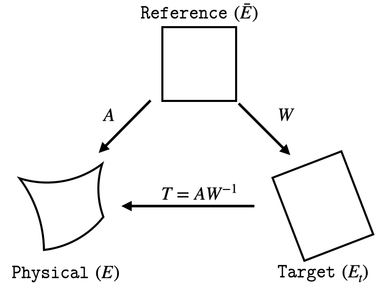
where $E_{t}$ are user-defined target elements through their Jacobian matrices $W_{d\times d}$; $T=AW^{-1}$ is the weighted Jacobian matrix from target to physical coordinates, see Figure 1; $\mu(T)$ is a mesh quality metric that defines a measure of the difference between the target and the physical geometric properties at a given location. The above configuration is the classical TMOP setup that is used as a backbone of many other mesh optimization methods [8, 24]. The term $F_{\sigma}(\boldsymbol{x})$ is the subject of this paper and will be discussed in Section 3. This term is used to enforce both tangential relaxation and surface fitting.

Figure 1: Schematic representation of the target to physical transformation in TMOP.

The objective function (4) is minimized by solving $\partial F(\boldsymbol{x})/\partial\boldsymbol{x}=\boldsymbol{0}$. This is done by a global nonlinear solve that modifies all values in $\boldsymbol{x}$ at once. Each iteration is enhanced by a line search procedure to ensure mesh validity, as described in [25]. Note that we typically use the Newton’s method, but occasionally we also employ the limited memory Broyden–Fletcher–Goldfarb–Shanno (L-BFGS) method. The convergence criterion for the solver is based on the norm of the gradient of the objective function with respect to the current and the initial mesh, $|\nabla F(\boldsymbol{x})|/|\nabla F(\boldsymbol{x}_{0})|\leq\varepsilon$, and we set $\varepsilon=10^{-6}$ for all the numerical results in this paper. For the case of Newton, the linear system inside each iteration is inverted by the standard minimum residual (MINRES) algorithm with an $l_{1}$ - Jacobi preconditioner.

3 Adaptive Surface Fitting and Tangential Relaxation

The main input of the method is a scalar FE function $\sigma_{0}(\boldsymbol{x_{0}})$ defined with respect to the initial mesh $\mathcal{M}_{0}$. The zero level set of this function specifies the surface of interest. In the following discussion we focus explicitly on the discrete case, but the method is also applicable when $\sigma$ is given analytically. The proposed algorithm is nearly identical for the cases of fitting and tangential relaxation; we will generally not separate the two cases, and the differences between them will be noted explicitly.

A starting step of the algorithm is to choose a subset of the mesh nodes, $\mathcal{S}$, which will be constrained on the zero level set. For the case of tangential relaxation (when we try to preserve a mesh surface), $\mathcal{S}$ is known by definition, as the surface of interest is defined by some of the faces of $\mathcal{M}_{0}$. The set $\mathcal{S}$ is also known when one wants to fit boundary faces of a non-aligned initial mesh. For the case of fitting a non-aligned initial mesh to an internal surface, however, choosing the set $\mathcal{S}$ can be a nontrivial problem, which we do not address in this paper. In our fitting tests we choose $\mathcal{S}$ through heuristics related to the shape of interest.

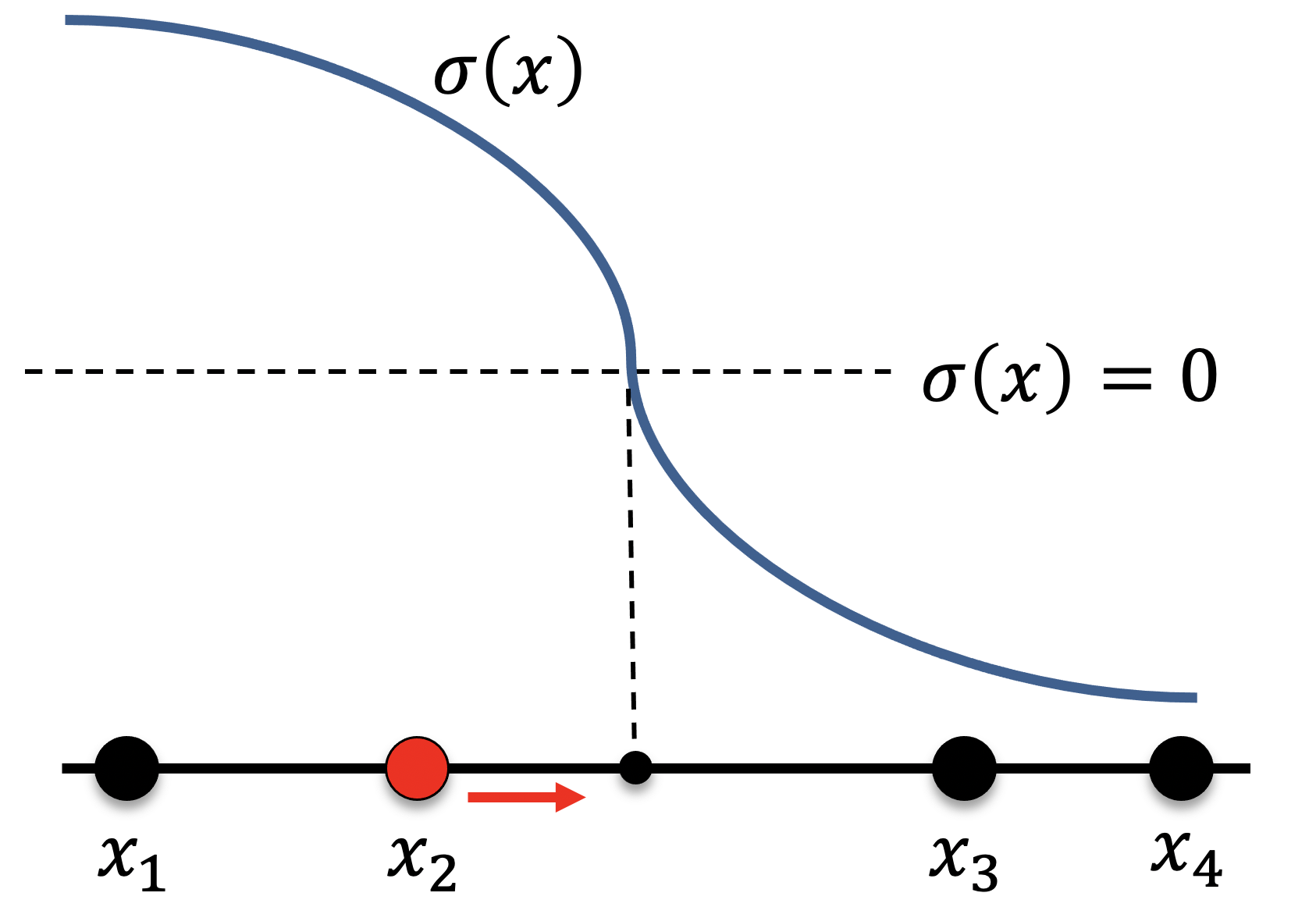
Once the set $\mathcal{S}$ is determined, the main idea of the adaptive surface alignment is to (i) move the mesh in a manner that leads to $\sigma(\boldsymbol{x_{s}})$ = 0, for all $s\in\mathcal{S}$, i.e., to place all nodes $s\in\mathcal{S}$ as close as possible to the zero level set, and (ii) to maintain optimal mesh quality as defined by the quality metric $\mu$. As there is no pre-determined unique target position for each node of $\mathcal{S}$, the method naturally allows tangential relaxation along the interface of interest. Simple 1D scheme illustration of the approach is shown in Figure 2, where the mesh node $\boldsymbol{x_{2}}$ is fitted to the zero level set of $\sigma$. For the 2D and 3D cases the level set becomes a curve and a surface, respectively.

Figure 2: Schematic representation of aligning mesh nodes to the zero level set of a discrete function.

The method is called adaptive, as the optimal mesh positions are obtained from a discrete function that comes from the simulation of interest. One of the main difficulties in this case comes from the fact that $\sigma$ is only defined with respect to the initial mesh. For a node $s\in\mathcal{S}$, let $\boldsymbol{x_{s0}}$ be its position in the initial mesh $\mathcal{M}_{0}$, and let $\boldsymbol{x_{s}}$ be its corresponding mesh position in the current mesh $\mathcal{M}$ which is evolving during the optimization. Generally $\sigma_{0}(\boldsymbol{x_{s0}})\neq 0$, as the chosen nodes may not originally be on the zero level set. After each mesh modification, we recompute a function $\sigma(\boldsymbol{x})$ on the new mesh (see additional details in Section 3.2), so that ideally $\sigma(\boldsymbol{x})=\sigma_{0}(\boldsymbol{x})$ for all points $\boldsymbol{x}$, which represents equivalence of $\sigma_{0}$ and $\sigma$ physical space.

Let the FE representation of $\sigma$ be

$$\sigma(\boldsymbol{x})=\sum_{i=1}^{N_{\phi}}\sigma_{i}\phi_{i}(\boldsymbol{x}),$$

where $\{\phi\}_{i=1}^{N_{\phi}}$ are the basis functions and $N_{\phi}$ is the total number of DOFs of $\sigma$. We make two important assumptions about the FE space of $\sigma$, namely:

• The FE space of $\sigma$ uses interpolatory basis functions, i.e., $\phi_{j}(\boldsymbol{x_{i}})=\delta_{ij}$ for all nodes $\boldsymbol{x_{i}}$, so that $\sigma(\boldsymbol{x_{i}})$ = 0 if and only if $\sigma_{i}=0$.

• The FE nodes of $\sigma$ and $\boldsymbol{x}$ coincide. For example, if the mesh control points are based on the Gauss-Lobatto reference positions (as explained in Section 2), then the FE space of $\sigma$ must be based on the Gauss-Lobatto positions as well.

If the application provides a $\sigma$ function that does not satisfy the above, a FE projection operation on an appropriate space can be performed. The above assumptions provide a very convenient property, namely, that minimizing the absolute value of a FE coefficient $\sigma_{s}$, for a node $s\in\mathcal{S}$, would lead to approaching $\sigma(\boldsymbol{x_{s}})=0$ which would mean that the mesh node $\boldsymbol{x_{s}}$ is near the zero level set of $\sigma$; in other words, $\boldsymbol{x_{s}}$ would be aligned to the surface of interest. This property is used to formulate the penalty term $F_{\sigma}$ in (4).

To incorporate the idea of minimizing $\sigma_{s}$ into the objective function (4), we first define the restricted FE function $\bar{\sigma}(x)$, s.t. for each FE coefficient $i$ we have:

$$\bar{\sigma}_{i}=\begin{cases}\sigma_{i}&\text{if}~{}i\in\mathcal{S},\\ 0&\text{otherwise}.\end{cases}$$ (5)

In other words, $\bar{\sigma}(x)=\sum_{s\in\mathcal{S}}\sigma_{s}\phi_{s}(x)$. The extra penalty term in the objective function (4) is formulated as:

$$F_{\sigma}=\frac{\omega_{\sigma}}{c_{\sigma}}\int_{E_{t}}\bar{\sigma}(x)^{2},$$ (6)

where $\omega_{\sigma}$ is a user-defined weight, and $c_{\sigma}$ is a normalization constant. The normalization scaling is used to ensure that $F_{\sigma}$ is invariant with respect to mesh refinement and scaling of the domain:

$$\frac{1}{c_{\sigma}}=\begin{cases}\frac{1}{N_{E}}\frac{1}{V_{\Omega,avg}}=\frac{1}{V_{\Omega}}&\text{for volumetric targets},\\ \frac{1}{N_{E}}&\text{otherwise},\end{cases}$$

where $N_{E}$ and $V_{\Omega}$ are the total number of mesh elements and volume of the domain, respectively. Here by volumetric targets we refer to the target Jacobian matrices $W$ that contain volumetric information and their determinants have unit of volume.

The extra term in the objective function penalizes the nonzero values of $\sigma(x_{s})$ for all $s\in\mathcal{S}$. Minimizing this term represents weak enforcement of $\sigma(\boldsymbol{x_{s}})=0$, only for the nodes in $\mathcal{S}$, while ignoring the values of $\sigma$ for the nodes outside $\mathcal{S}$. Note that minimizing the final nonlinear objective function $F=F_{\mu}+F_{\sigma}$, see (4), would treat all nodes together, i.e., the nonlinear solver would make no explicit separation between surface and non-surface nodes.

Remark 1

Since the FE basis of $\boldsymbol{x}$ is also interpolatory, we can simply assume that the basis functions of $\sigma$ and $\boldsymbol{x}$ are the same, that is, $\phi\equiv w$. Throughout the paper we keep both notations to distinguish the terms related to $\sigma$ from the ones related to the mesh positions.

3.1 Derivatives

As our default choice for nonlinear optimization is the Newton’s method, we must compute two derivatives of $F_{\sigma}$ with respect to the mesh nodes. In this discussion we’re exclusively targeting the discrete case, when the level set function $\sigma(\boldsymbol{x})$ is a discrete FE function. All derived formulas are also applicable to the analytic case; a remark about the required modification is given at the end of the section.

Let the FE expansion for $\sigma$ be $\sigma(\boldsymbol{x})=\sum_{k}\sigma_{k}\phi_{k}(\boldsymbol{x})$, and let the FE position function be $\boldsymbol{x}=(x_{1}\dots x_{d})^{T}$ where $d$ is the dimension and each component can be written as $x_{a}=\sum_{i}x_{a,i}w_{i}(\boldsymbol{\bar{x}})$. For a node $s\in\mathcal{S}$, let $\boldsymbol{x_{s}}$ be its position. As the chosen FE basis is interpolatory, we have $\boldsymbol{x_{s}}=(x_{1,s}\dots x_{d,s})^{T}$, and we can write the following equivalence:

$$\sigma_{s}=\sigma(\boldsymbol{x_{s}})=\sum_{k=1}^{N_{x}}\sigma_{k}\phi_{k}(\boldsymbol{x_{s}}),\quad\text{since}\quad\phi_{k}(\boldsymbol{x_{s}})=\delta_{ks}.$$

Thus we can rewrite $\bar{\sigma}$ as

$$\bar{\sigma}(\boldsymbol{x})=\sum_{s\in\mathcal{S}}\sigma_{s}\phi_{s}(\boldsymbol{x})=\sum_{s\in\mathcal{S}}\sum_{k=1}^{N_{x}}\sigma_{k}\phi_{k}(\boldsymbol{x_{s}})\phi_{s}(\boldsymbol{x}).$$

The above formula is useful for derivative computations. Namely, we have $\phi_{k}(\boldsymbol{x_{s}})=0$ when $k\neq s$, however, the derivatives $\partial\phi_{k}(\boldsymbol{x_{s}})/\partial\boldsymbol{x}\neq 0$. A chain rule for the above expression (given below) expresses how the change of the DOF values $\sigma(\boldsymbol{x_{s}})$ contribute to the change of the quadrature point values of the restricted FE function $\bar{\sigma}(\boldsymbol{x})$. The formulas for the first and second derivatives of $F_{\sigma}$ are the following:

$$\begin{split}\frac{\partial F_{\sigma}}{\partial x_{a,i}}=\frac{2\omega_{\sigma}}{c_{\sigma}}\int_{E_{t}}&\bar{\sigma}(\boldsymbol{x})\frac{\partial\bar{\sigma}(\boldsymbol{x})}{\partial x_{a}}\frac{\partial x_{a}}{\partial x_{a,i}}\\ =\frac{2\omega_{\sigma}}{c_{\sigma}}\int_{E_{t}}&\bar{\sigma}(\boldsymbol{x})\sum_{s\in\mathcal{S}}\sum_{k}\sigma_{k}\bigg{(}\frac{\partial\phi_{k}(\boldsymbol{x_{s}})}{\partial x_{a}}\phi_{s}(\boldsymbol{x})+\\ &\qquad\qquad\qquad\phi_{k}(\boldsymbol{x_{s}})\frac{\partial\phi_{s}(\boldsymbol{x})}{\partial x_{a}}\bigg{)}w_{i}(\boldsymbol{\bar{x}}),\end{split}$$

$$\begin{split}\frac{\partial^{2}F_{\sigma}}{\partial x_{b,j}\partial x_{a,i}}=\frac{2\omega_{\sigma}}{c_{\sigma}}\int_{E_{t}}&\bigg{(}\frac{\partial\bar{\sigma}(\boldsymbol{x})}{\partial x_{b}}\frac{\partial\bar{\sigma}(\boldsymbol{x})}{\partial x_{a}}+\\ &\quad\bar{\sigma}(\boldsymbol{x})\frac{\partial^{2}\bar{\sigma}(\boldsymbol{x})}{\partial x_{b}\partial x_{a}}\bigg{)}\frac{\partial x_{a}}{\partial x_{a,i}}\frac{\partial x_{b}}{\partial x_{b,i}}\\ =\frac{2\omega_{\sigma}}{c_{\sigma}}\int_{E_{t}}&\left(\mathcal{D}_{a}\mathcal{D}_{b}+\bar{\sigma}(\boldsymbol{x})\mathcal{D}^{2}\right)w_{i}(\boldsymbol{\bar{x}})w_{j}(\boldsymbol{\bar{x}}),\end{split}$$

where

$$\begin{split}\mathcal{D}_{*}=\sum_{s\in\mathcal{S}}\sum_{k}&\sigma_{k}\left(\frac{\partial\phi_{k}(\boldsymbol{x_{s}})}{\partial x_{*}}\phi_{s}(\boldsymbol{x})+\phi_{k}(x_{s})\frac{\partial\phi_{s}(\boldsymbol{x})}{\partial x_{*}}\right),\\ \mathcal{D}^{2}=\sum_{s\in\mathcal{S}}\sum_{k}&\sigma_{k}\bigg{(}\frac{\partial\phi_{k}(\boldsymbol{x_{s}})}{\partial x_{a}}\frac{\partial\phi_{s}(\boldsymbol{x})}{\partial x_{b}}+\frac{\partial^{2}\phi_{k}(\boldsymbol{x_{s}})}{\partial x_{b}\partial x_{a}}\phi_{s}(\boldsymbol{x})~{}+\\ &\quad\frac{\partial\phi_{k}(\boldsymbol{x_{s}})}{\partial x_{b}}\frac{\partial\phi_{s}(\boldsymbol{x})}{\partial x_{a}}+\phi_{k}(\boldsymbol{x_{s}})\frac{\partial^{2}\phi_{s}(\boldsymbol{x})}{\partial x_{b}\partial x_{a}}\bigg{)},\end{split}$$

$$a,b=1\dots d,\quad i,j=1\dots N_{x}.$$

The above integrals are approximated by a standard Gauss-Lobatto integration rule of order that depends on the used mesh degree. Note that the above formulas mix gradients at quadrature points, e.g., $\partial\phi_{s}(\boldsymbol{x})/\partial x_{a}$, and gradients at the nodes of $\mathcal{S}$, e.g., $\partial\phi_{k}(\boldsymbol{x_{s}})/\partial x_{a}$. Furthermore, note that gradients of the basis functions are with respect to physical coordinates, s.t. integration in reference space would require to compute $\nabla\phi(\boldsymbol{x})=A^{-T}\nabla\hat{\phi}(\boldsymbol{\bar{x}})$. This leads to more involved computations of the second derivatives. One possibility to avoid this is to utilize approximate second derivatives, which are obtained through repeated application of the FE discrete gradient operator.

Analytic case. When $\sigma(\boldsymbol{x})$ is prescribed analytically, the above formulas still hold with a slight simplification. In this case it is more convenient to rewrite the restricted function $\bar{\sigma}(\boldsymbol{x})$ as

$$\bar{\sigma}(\boldsymbol{x})=\sum_{s\in\mathcal{S}}\sigma(\boldsymbol{x_{s}})\phi_{s}(\boldsymbol{x}).$$

Then the first derivative of $F_{\sigma}$ becomes:

$$\begin{split}\frac{\partial F_{\sigma}}{\partial x_{a,i}}=\frac{2\omega_{\sigma}}{c_{\sigma}}\int_{E_{t}}&\bar{\sigma}(\boldsymbol{x})\frac{\partial\bar{\sigma}(\boldsymbol{x})}{\partial x_{a}}\frac{\partial x_{a}}{\partial x_{a,i}}\\ =\frac{2\omega_{\sigma}}{c_{\sigma}}\int_{E_{t}}&\bar{\sigma}(\boldsymbol{x})\sum_{s\in\mathcal{S}}\bigg{(}\frac{\partial\sigma(\boldsymbol{x_{s}})}{\partial x_{a}}\phi_{s}(\boldsymbol{x})+\\ &\qquad\qquad\sigma(\boldsymbol{x_{s}})\frac{\partial\phi_{s}(\boldsymbol{x})}{\partial x_{a}}\bigg{)}w_{i}(\boldsymbol{\bar{x}}),\end{split}$$

where all derivatives $\partial\sigma(\boldsymbol{x})/\partial x_{a},a=1\dots d$ are known analytically. The formulas for the second derivatives are modified in a similar manner.

3.2 Interpolation Between Meshes

As we always use an iterative method that produces a sequence of meshes, we need to compute $\sigma(\boldsymbol{x})$ and its gradients on any of these meshes. This is straightforward when $\sigma$ is given analytically, but in practice, $\sigma$ is often a discrete function produced by a numerical simulation. As such, it is only defined with respect to the initial mesh $\mathcal{M}_{0}$. In these cases the ability to compute $\sigma(\boldsymbol{x})$ on an evolved mesh $\mathcal{M}$ is a major requirement for the algorithm. An exact equivalence in physical space would mean to have $\sigma(\boldsymbol{x})=\sigma_{0}(\boldsymbol{x})$ for all points $\boldsymbol{x}$, but this is not possible due to the discrete FE representation of these functions.

The reconstruction of $\sigma$ on $\mathcal{M}$ can be performed entirely by FE operations. Using the topological equivalence of $\mathcal{M}_{0}$ and $\mathcal{M}$, one can define mesh velocity $\boldsymbol{v}=\boldsymbol{x}-\boldsymbol{x_{0}}$ and solve the following advection PDE in pseudo-time $\tau\in[0,1]$:

$$\frac{d\sigma(\boldsymbol{x}_{\tau},\tau)}{d\tau}=\boldsymbol{u}\nabla\sigma(\boldsymbol{x}_{\tau},\tau)\cdot,\quad\sigma(\boldsymbol{x}_{0},0)=\sigma_{0}(\boldsymbol{x}_{0}),$$

where $\boldsymbol{x}_{\tau}=\boldsymbol{x}_{0}+\tau\boldsymbol{v}$. Further details about this procedure can be found in Section 4.2 of [22].

Another option is high-order interpolation between meshes in physical space, which is enabled by the open-source library, gslib [26]. The findpts set of routines in gslib provide two key functionalities. First, for a given set of points in physical space, findpts determines the computational coordinates for each point, i.e., the element $E$ which contains the point and the reference-space coordinate $\boldsymbol{\bar{x}}$ inside the corresponding reference element $\bar{E}$. Second, using the computational coordinates, any given high-order FE function is interpolated (1). These two key functionalities allow the transfer of a high-order FE function from one mesh onto another. The reader is referred to Section 2.3 of [27] for further details.

4 Numerical Examples

In this section we demonstrate the main properties of the method on several proof-of-concept 2D and 3D tests. We start with standard surface fitting tests on different element types, followed by treatment of smooth and non-smooth internal interfaces. Extensive evaluation of the proposed method on more complicated geometries and practical problems will be performed in future work, as these cases require additional capabilities that are not established yet in our software. Nevertheless, the proposed method can be readily utilized as a building block by other established mesh optimization frameworks like [8, 24].

Unless notes otherwise, the presented tests utilize the following composite mesh quality metrics:

$$\begin{split}\mu_{80}&=(1-\gamma)\mu_{2}+\gamma\mu_{77},\\ \mu_{333}&=(1-\gamma)\mu_{302}+\gamma\mu_{316},\end{split}$$ (7)

where $\gamma=0.5$ and

$$\begin{split}\mu_{2}&=0.5\frac{|T|^{2}}{\tau}-1,\quad\quad\mu_{77}=0.5\left(\tau-\frac{1}{\tau}\right)^{2},\\ \mu_{302}&=\frac{|T|^{2}|T^{-1}|^{2}}{9}-1,\quad\mu_{316}=0.5\left(\tau+\frac{1}{\tau}\right)-1,\end{split}$$

where $|T|$ and $\tau$ are the Frobenius norm and determinant of $T$, respectively. The metric $\mu_{80}$ is a 2D shape+size metric, while $\mu_{333}$ is a 3D shape+size metric. Both are polyconvex in the sense of [28, 29], i.e., the metric integral $F_{\mu}$ in (4) theoretically has a minimizer. A thorough investigation of the theoretical properties of the above (and many other) mesh quality metrics and metric types can be found in [30]. Exploring how the smoothness properties of $\sigma$ affect the convexity properties of the full objective function $F=F_{\mu}+F_{\sigma}$ will be the subject of future studies.

Our implementation utilizes the MFEM finite element library [3]. This implementation is freely available at https://mfem.org.

4.1 2D Surface Fitting

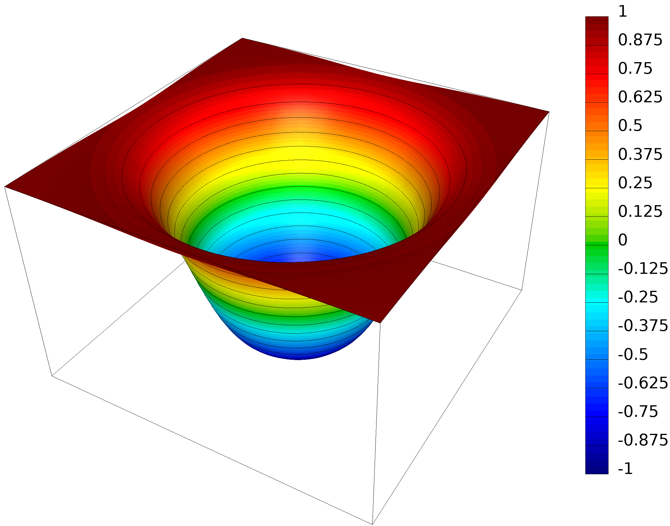
As a first example, we perform surface fitting to 3rd order 2D meshes consisting of quads and triangles, see Figure 4. For both meshes we use TMOP with tangential relaxation and fitting capability (4)-(6) to adapt the internal interface to the zero level-set of a function. The zero level-set of the function $\sigma$ is defined such that it is located at a distance of 0.3 from the center of the domain, $\boldsymbol{x}_{c}=(0.5,0.5)$, see Figure 3. Although this level set is known analytically, the presented computations represent and use $\sigma$ as a discrete finite element function.

Figure 3: Level set function $\sigma$ that is used for the 2D surface fitting tests.

$\begin{array}[]{ccc}\includegraphics[height=93.94955pt]{figures/2D-quad}&\includegraphics[height=93.94955pt]{figures/2D-tri}\end{array}$

Figure 4: Initial quadrilateral / triangle meshes and internal interfaces for the 2D surface fitting tests.

$\begin{array}[]{cc}\includegraphics[height=93.94955pt]{figures/2D-quad-opt}&\includegraphics[height=93.94955pt]{figures/2D-tri-opt}\\ \end{array}$

Figure 5: Optimized quadrilateral and triangle meshes for the 2D surface fitting tests.

For both meshes we set $w_{\sigma}=1000$. The target matrix $T$ is chosen to represent an ideal element (square or equilateral triangle), and we use the shape-only metric

$$\mu_{58}(T)=\frac{|T^{t}T|^{2}}{\tau^{2}}-{2|T|^{2}}{\tau}+2.$$

The optimized meshes are shown in Figure 5. For the quadrilateral case, the TMOP objective function $F(\boldsymbol{x})$ decreases by $61.8\%$; for the triangular case, $F(\boldsymbol{x})$ decreases by $71.9\%$. For each of the optimized meshes, we also measure the average error for the degree-of-freedoms associated with the material interface as

$$e_{\mathcal{S}}=\frac{\sum_{s\in\mathcal{S}}\bigg{(}||(\boldsymbol{x_{s}}-\boldsymbol{x}_{c})||_{2}-0.3\bigg{)}^{2}}{\sum_{s\in\mathcal{S}}1},$$ (8)

where $\mathcal{S}$ is the set of nodes chosen to align to the interface, $\boldsymbol{x_{s}}$ denotes the physical-location of the node $s$, and $||\cdot||_{L_{2}}$ denotes the $L_{2}$-norm of a vector. We observe that the average error at the zero-level set is $O(10^{-6})$ for each of the meshes.

4.2 3D Surface Fitting

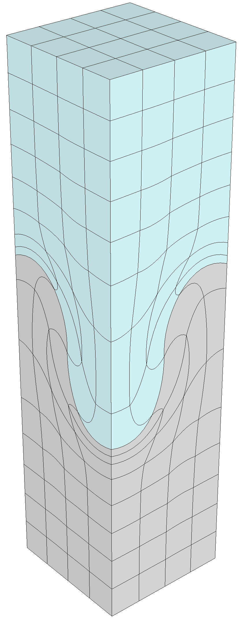
Next we consider the analogous 3D case and perform surface fitting to 2nd order 3D meshes consisting of hexes and tets. Figure 6 shows a sliced-view of the meshes, where the element colors denote the two sides of the internal interface. For both meshes the zero level set of the function $\sigma$ is at a distance of 0.3 from the center of the domain $\boldsymbol{x}_{c}=(0.5,0.5,0.5)$. We set $w_{\sigma}=1000$. The target matrix $T$ is chosen to represent an ideal element (cube or equilateral tetrahedron) with size target based on the size of the elements in the original mesh. The mesh quality is controlled by the polyconvex shape+size metric $\mu_{333}(T)$.

$\begin{array}[]{cc}\includegraphics[height=108.04163pt]{figures/3D-hex}&\includegraphics[height=108.04163pt]{figures/3D-tet}\\ \end{array}$

Figure 6: Initial hexahedral / tetrahedral meshes and internal interfaces for the 3D surface fitting tests.

$\begin{array}[]{cc}\includegraphics[height=103.34666pt]{figures/3D-hex-opt}&\includegraphics[height=103.34666pt]{figures/3D-tet-opt}\\ \end{array}$

Figure 7: Optimized hexahedral and tetrahedral meshes for the 3D surface fitting tests.

The optimized meshes are shown in Fig. 7. For the mesh with hexahedral elements, we observe that $F(\boldsymbol{x})$ reduces by $91.4\%$, and the error at the zero level-set (8) is $O(10^{-5})$. For the mesh with tetrahedrons, $F(\boldsymbol{x})$ reduces by $78.7\%$, with $e_{\mathcal{S}}=O(10^{-6})$. The error at the zero level-set is relatively higher for the mesh with hexahedral elements due to the mesh topology. The hex mesh has elements that have more than one face at the material interface, which would have to tangentially flatten along the zero level-set to exactly satisfy the surface fitting term (6). Since this would result in an inverted mesh, the mesh optimizer fits the mesh the best it can while ensuring mesh quality based on the metric $\mu_{333}(T)$ used in the first term of (4).

4.3 Taylor-Green Interface

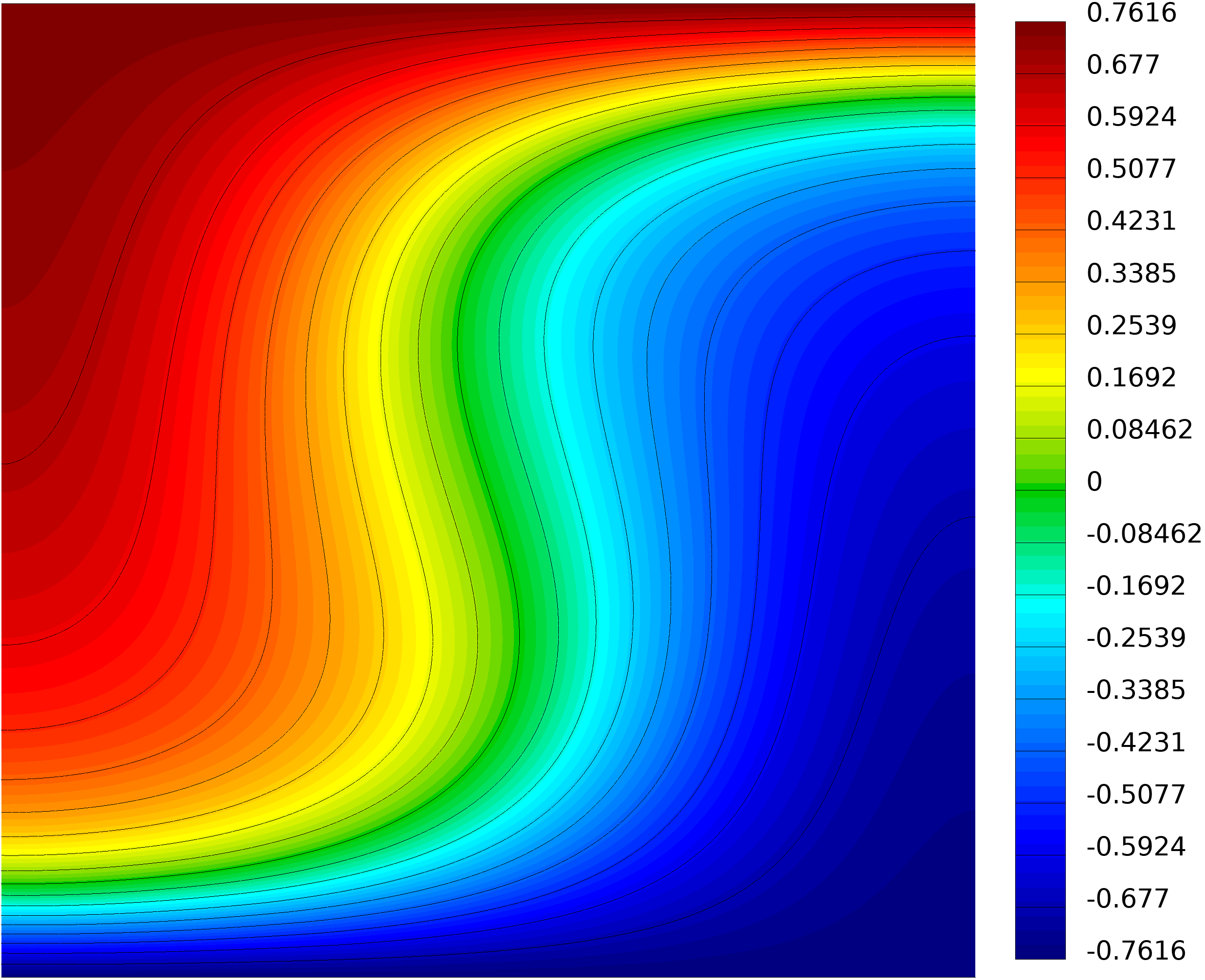
The primary target application of our work are multimaterial moving mesh simulations. In this context, a common goal of the mesh optimization procedure is to improve the mesh while preserving an initially aligned material interface. In this example we start with a 3rd order mesh and a material interface obtained from a Taylor-Green moving mesh simulation [31]. The level set function $\sigma(\boldsymbol{x})$ is shown in Figure 8; the initial mesh is shown in the top left panel of Figure 9.

We compare results from three different setups, namely (i) fixing the interface nodes during the optimization, (ii) tangential relaxation with $w_{\sigma}=250$, and (iii) tangential relaxation with $w_{\sigma}=1000$. The decrease in the objective function and the interface position errors are listed in Table 1, while the optimized meshes for the three cases are shown in Figure 9. In all cases the mesh quality is controlled by the quality metric $\mu_{80}$, and the target Jacobians represent ideally shaped elements that maintain their initial local size. Since $\sigma$ is not known analytically, the interface position errors are defined with respect to the violation of the zero level set:

$$\mathcal{E}_{avg}=\frac{1}{|\mathcal{S}|}\sum_{s\in\mathcal{S}}\bar{\sigma}(\boldsymbol{x_{s}}),\quad\mathcal{E}_{max}=\max_{s\in\mathcal{S}}\bar{\sigma}(\boldsymbol{x_{s}}).$$

Approach	$F$ decrease	$\mathcal{E}_{avg}$	$\mathcal{E}_{max}$
Fixed interface	34.4%	0	0
$w_{\sigma}=250$	51.4%	8.2e-2	1.3e-1
$w_{\sigma}=1000$	42.6%	3.6e-2	6.4e-2

Table 1: Comparison of optimization strategies for the 2D Taylor-Green test.

We observe that the parameter $w_{\sigma}$ has the expected influence on the fitting accuracy, namely, increasing its value leads to better agreement with the zero level set of $\sigma$. On the other hand, smaller values of $w_{\sigma}$ give more freedom to the interface nodes, leading to better mesh quality at the price of increased error of the interface positions. Finally, completely fixing the interface nodes gives the lowest quality mesh, as the optimizer has no control over the interfacial nodes.

Figure 8: Level sets of the finite element function $\sigma(\boldsymbol{x})$ for the material interface arising in the Taylor-Green test.

Figure 9: Top row: initial mesh (left) and optimized mesh with fully constrained interface nodes (right). Bottom row: optimized mesh with $w_{\sigma}=250$ (left) and optimized mesh with $w_{\sigma}=1000$ (right).

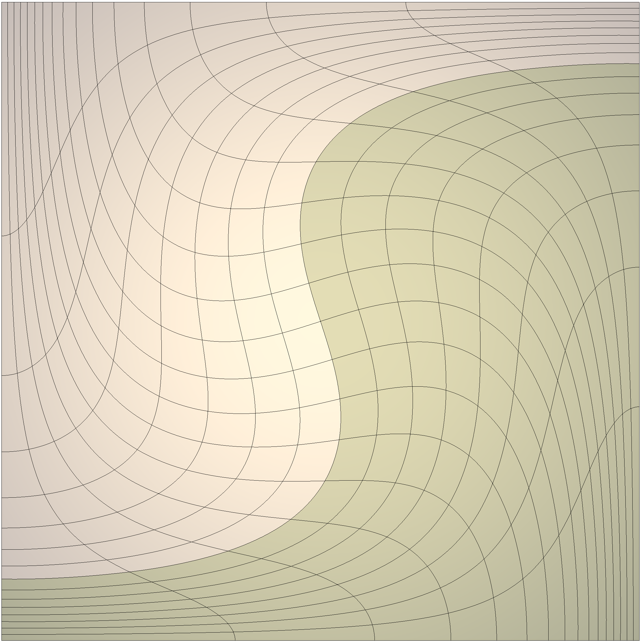
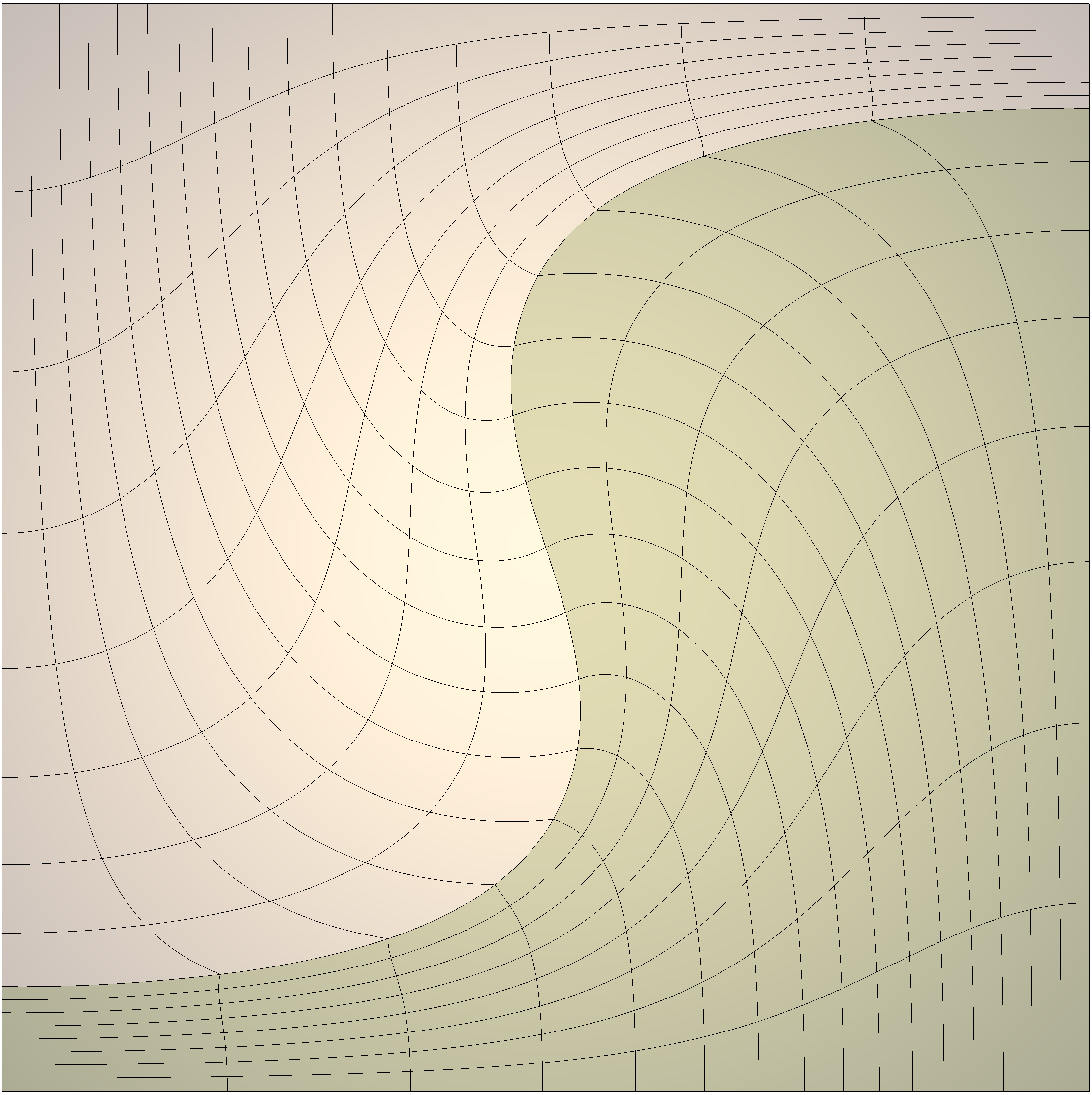
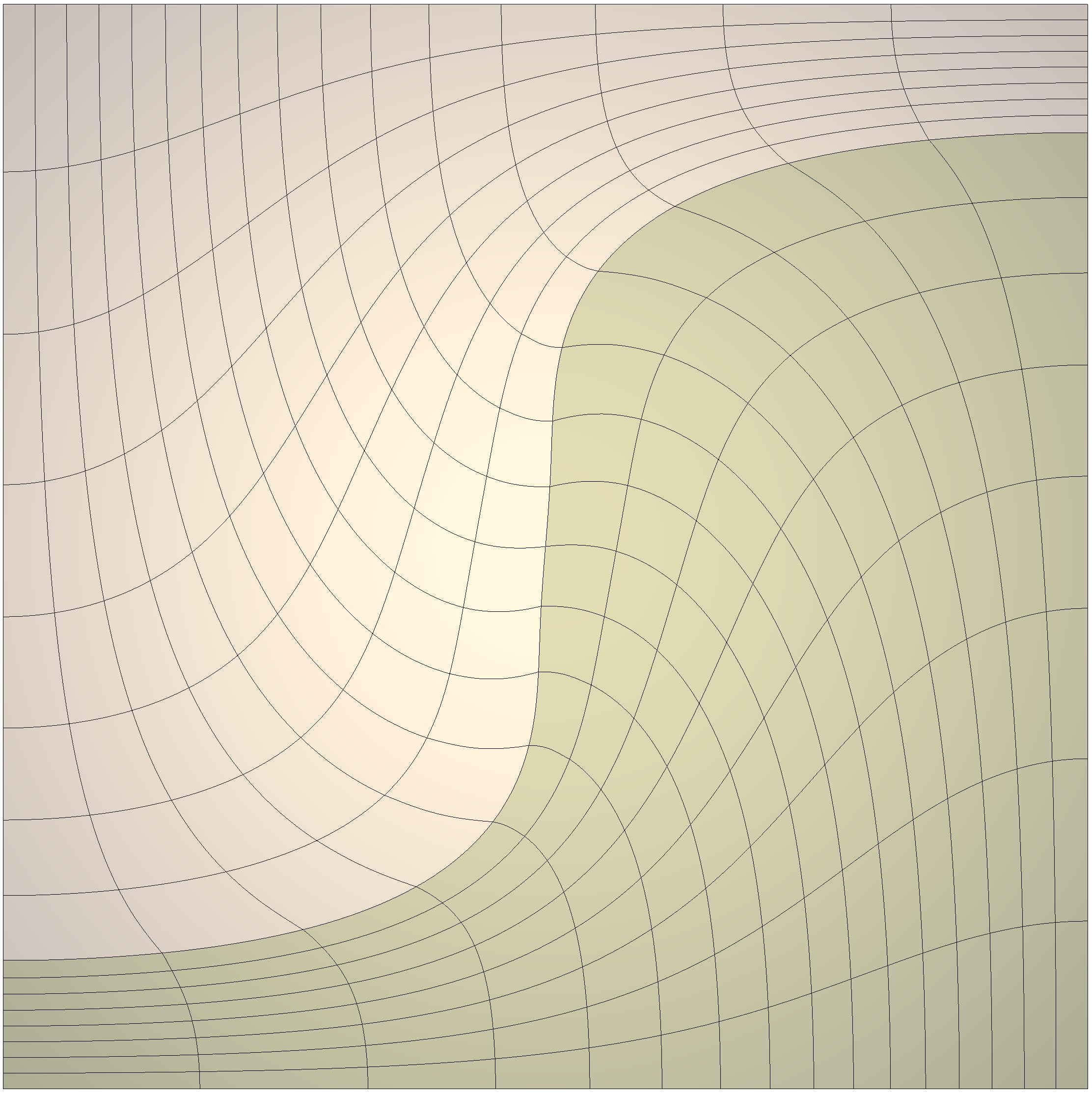
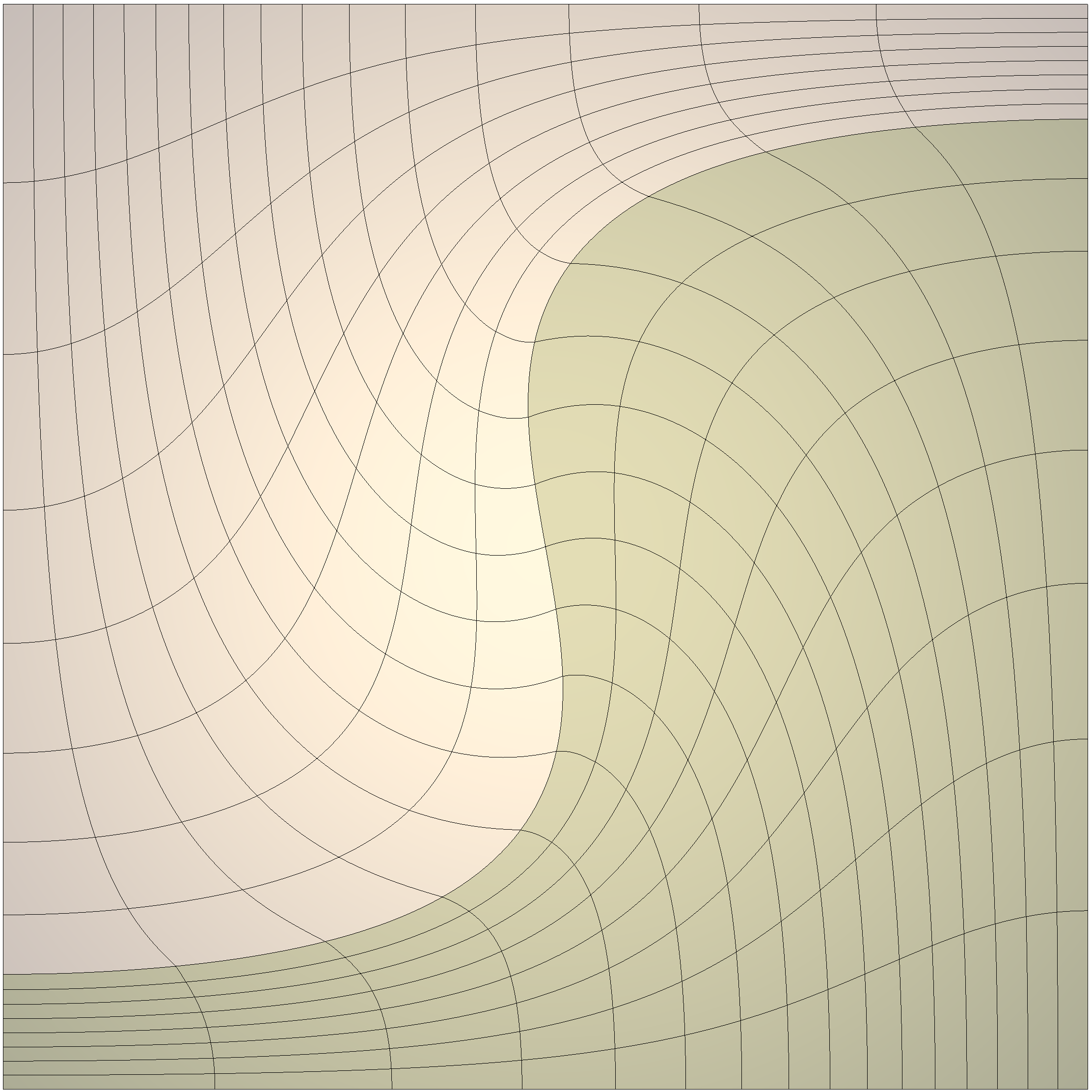
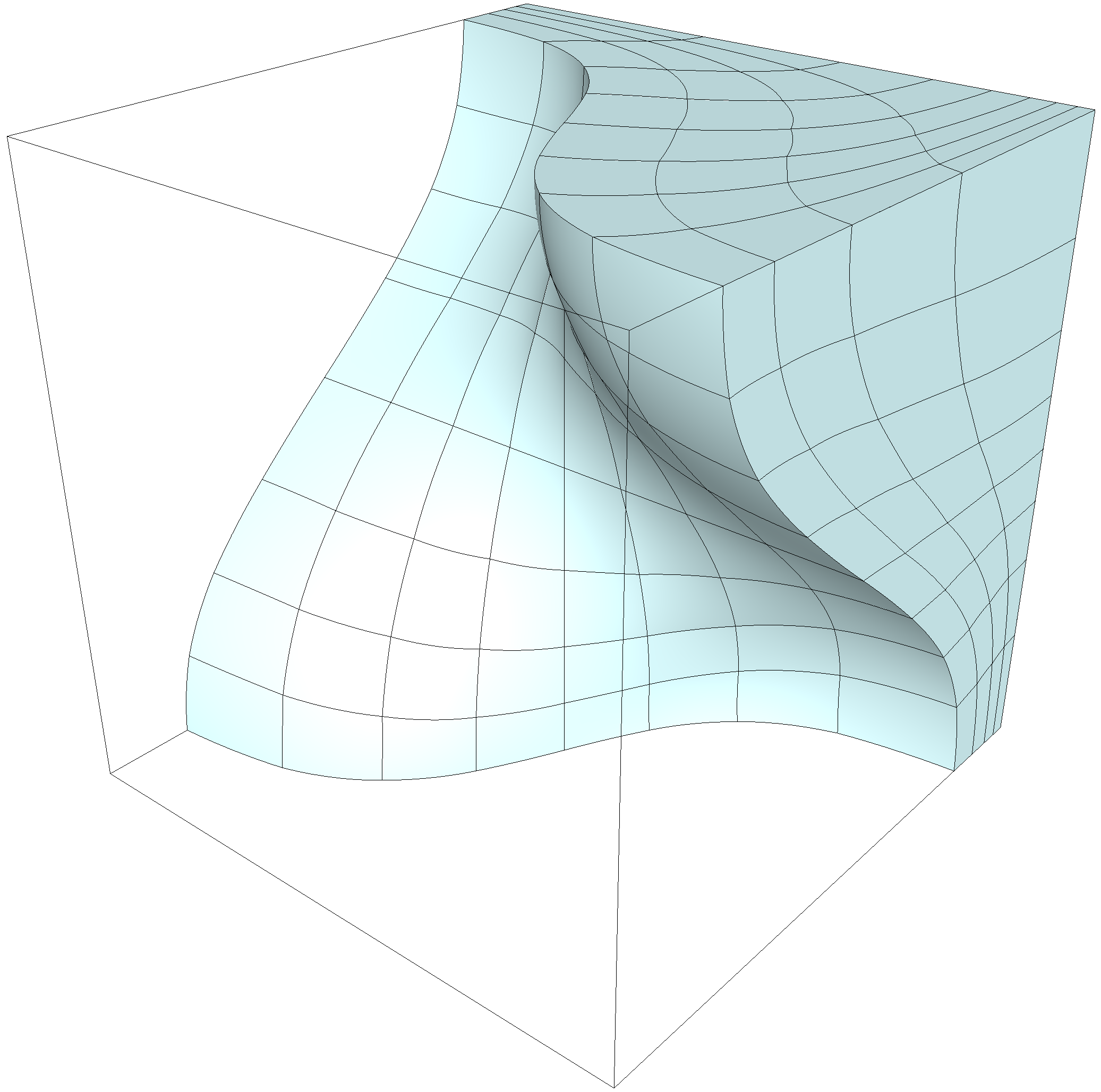
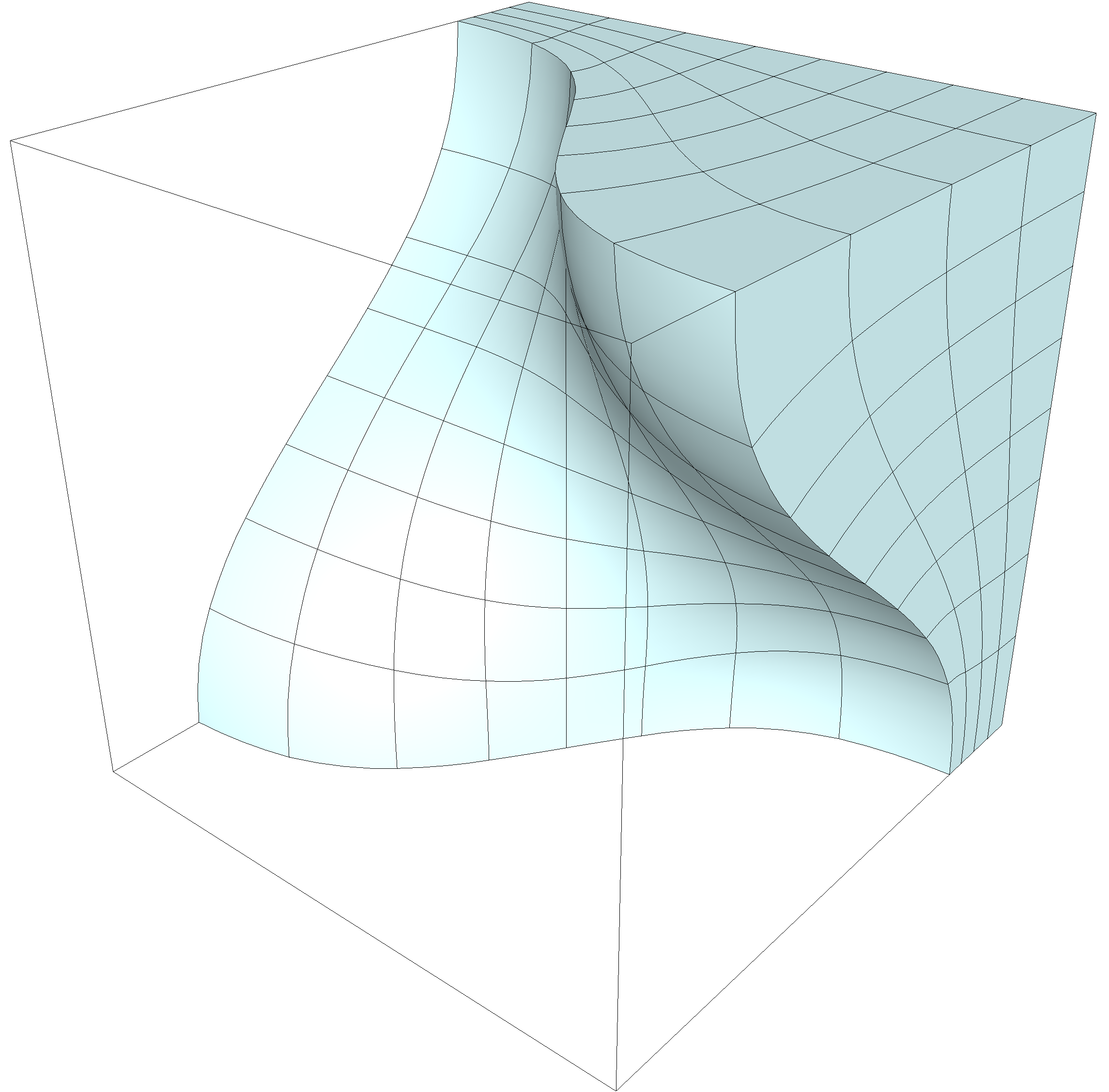
The 3D version of the same problem is presented in Figure 10, where we show cuts (along the material interface) of the initial mesh and the optimized mesh with $w_{\sigma}=1000$. The 3D comparison between the above three optimization strategies is listed in Table 2. The 3D results confirm the observations made in the 2D tests.

Approach	$F$ decrease	$\mathcal{E}_{avg}$	$\mathcal{E}_{max}$
Fixed interface	54.5%	0	0
$w_{\sigma}=250$	72.7%	4.9e-2	1.5e-1
$w_{\sigma}=1000$	63.6%	1.7e-2	6.2e-2

Table 2: Comparison of optimization strategies for the 3D Taylor-Green test.

Figure 10: Initial mesh (top) and optimized mesh with $w_{\sigma}=1000$ (bottom) for the material interface arising in the 3D Taylor-Green test.

4.4 Rayleigh-Taylor Interface

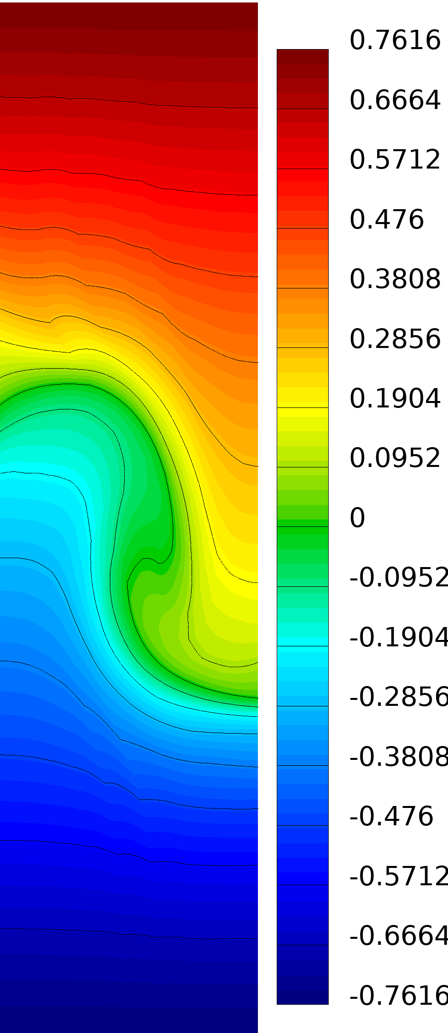
Next we consider the Rayleigh-Taylor two-material problem [6], where the dynamics of the system leads to an interface that is not smooth. The goal of this test is to demonstrate the behavior of the method for non-smooth surfaces that contain fine local features. The initial 2nd order mesh and the level set function $\sigma(\boldsymbol{x})$ are shown in Figure 11.

Again we utilize the $\mu_{80}$ quality metric and the target Jacobians represent ideally shaped elements that maintain their initial local size. Optimizing the mesh by exactly preserving the positions of the interfacial nodes leads to a 38.6% decrease in the objective function $F(\boldsymbol{x})$, while optimizing with $w_{\sigma}$ = 1.0e4 leads to a decrease of 52.5%, with $\mathcal{E}_{avg}$ = 9.9e-3 and $\mathcal{E}_{max}$ = 4.4e-2. The final optimized meshes for the two cases are shown in Figure 11.

Figure 11: Left to right: initial mesh, optimized mesh with fully constrained interface nodes, optimized mesh with $w_{\sigma}$ = 1.0e4, and level sets of the finite element function $\sigma(\boldsymbol{x})$ for the 2D Rayleigh-Taylor test.

Figure 12: Initial mesh and cut of the level set function $\sigma(\boldsymbol{x})$ for the 3D Rayleigh-Taylor test.

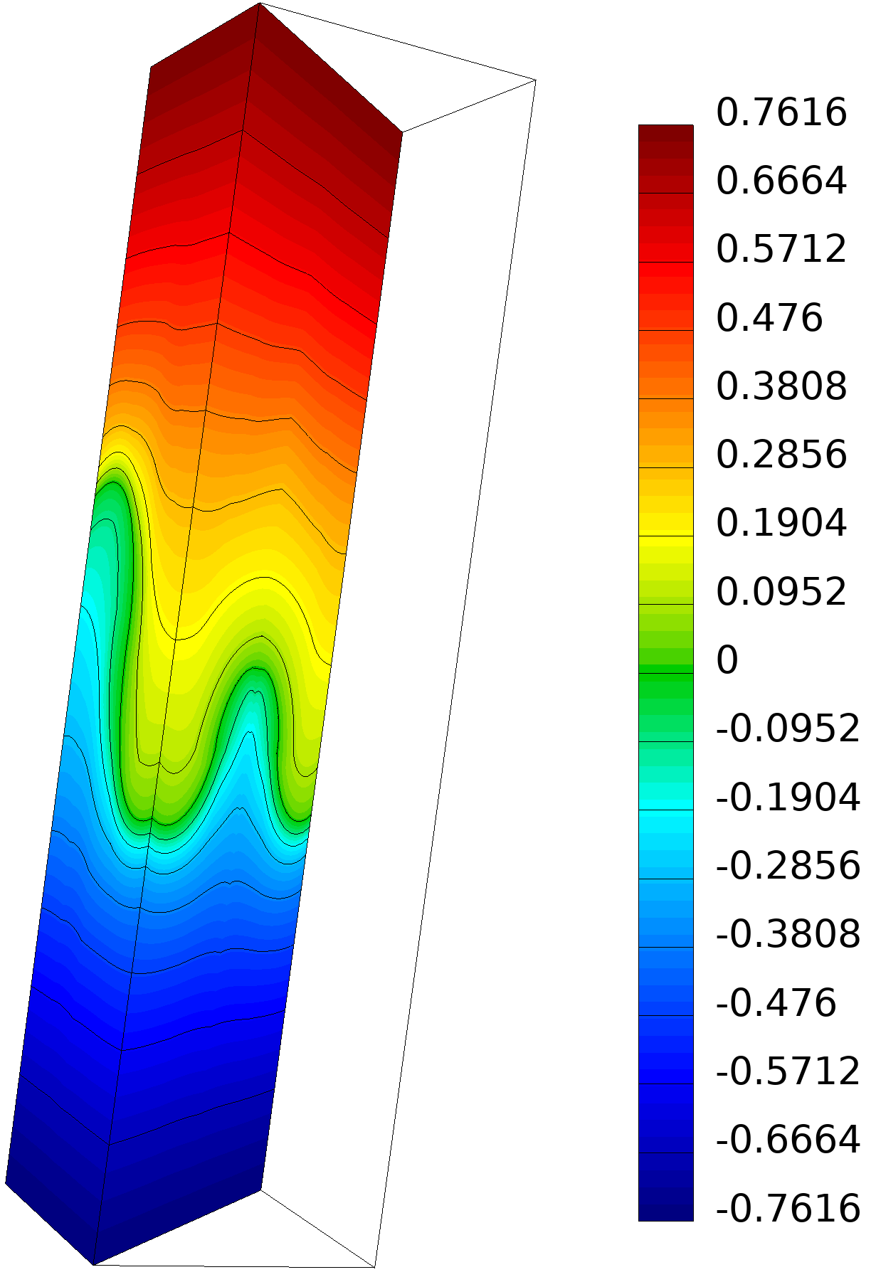
The above results demonstrate that the proposed method can lead to diffusion of small surface features, even when $w_{\sigma}$ is large. The reason is that the interface nodes $s\in\mathcal{S}$ are allowed to move anywhere where the function $\sigma(\boldsymbol{x_{s}})$ is small, as long as they improve the mesh quality $\mu(\boldsymbol{x})$ in their local neighborhood. Thus, small interface kinks as the ones visible in the left panel of Figure 11 can be eliminated without any significant resulting penalization in $F_{\sigma}$. This behavior can be mitigated by detecting the local features of the surface, e.g., by examining the gradients of $\sigma$, and performing localized treatments. For example, one can fix only specific nodes or increase the resolution around the feature by adapting the local size through $r$- or $h$-adaptivity [25]. Another approach to address the non-smoothness of $\sigma$ is to replace the function by $N_{c}$ smooth component functions $\sigma_{1}\dots\sigma_{N_{c}}$, and have a separate objective term for each smooth component in (4). This strategy can be seen as the discrete analogy of the virtual geometry surface decomposition models [15]. Exploring the above strategies will be the subject of future work.

Figure 13: Optimized mesh with fully constrained interface nodes (top) and optimized mesh with $w_{\sigma}$ = 1.0e4 (bottom) for the material interface arising in the 3D Rayleigh-Taylor test.

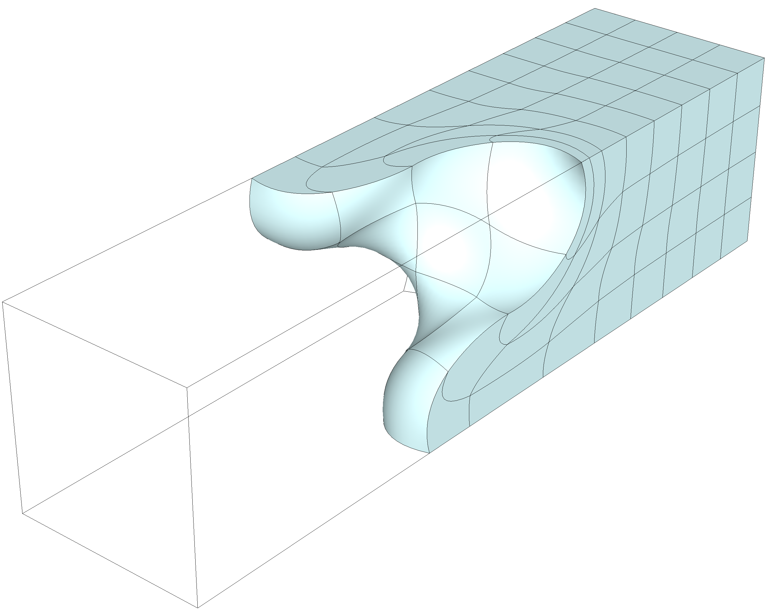
The 3D version of the same problem is presented in Figures 12 and 13, where we observe behavior similar to the 2D case. Optimizing the mesh by exactly preserving the positions of the interfacial nodes leads to a 51.5% decrease in the objective function $F(\boldsymbol{x})$, while optimizing with $w_{\sigma}$ = 1.0e4 leads to a decrease of 62.9%, with $\mathcal{E}_{avg}$ = 8.8e-3 and $\mathcal{E}_{max}$ = 3.8e-2.

5 Conclusion

We have presented a new approach to fit or align certain high-order mesh faces to a surface given by a discrete level set function. The alignment is imposed weakly by including a variational penalty term in the objective functional. The main advantage of the method is that its major steps can be implemented strictly through finite element operations without performing any geometric calculations, making the algorithm independent of dimension, mesh order, and element type. The main disadvantage of the algorithm is that local non-smooth surfaces may be diffused in the optimization process. Improving this aspect of the method will be future work, as discussed in Section 4.4.

In the future the method will also be extended to handle the case of boundary fitting, which is not addressed in this paper. This will likely be approached by utilizing an auxiliary background mesh. Extensive evaluation of the proposed method on larger problems with complicated geometries will also be performed, which will require robust strategies for combining several level set functions and more involved node marking algorithms.

Disclaimer

This document was prepared as an account of work sponsored by an agency of the United States government. Neither the United States government nor Lawrence Livermore National Security, LLC, nor any of their employees makes any warranty, expressed or implied, or assumes any legal liability or responsibility for the accuracy, completeness, or usefulness of any information, apparatus, product, or process disclosed, or represents that its use would not infringe privately owned rights. Reference herein to any specific commercial product, process, or service by trade name, trademark, manufacturer, or otherwise does not necessarily constitute or imply its endorsement, recommendation, or favoring by the United States government or Lawrence Livermore National Security, LLC. The views and opinions of authors expressed herein do not necessarily state or reflect those of the United States government or Lawrence Livermore National Security, LLC, and shall not be used for advertising or product endorsement purposes.

References

- [1] Deville M., Fischer P., Mund E. High-order methods for incompressible fluid flow. Cambridge University Press, 2002
- [2] Fischer P., Min M., Rathnayake T., Dutta S., Kolev T., Dobrev V., Camier J.S., Kronbichler M., Warburton T., Świrydowicz K., et al. “Scalability of high-performance PDE solvers.” The International Journal of High Performance Computing Applications, vol. 34, no. 5, 562–586, 2020
- [3] Anderson R., Andrej J., Barker A., Bramwell J., Camier J.S., Cerveny J., Dobrev V., Dudouit Y., Fisher A., Kolev T., et al. “MFEM: a modular finite element methods library.” Computers & Mathematics with Applications, vol. 81, 42–74, 2021
- [4] Kolev T., Fischer P., Min M., Dongarra J., Brown J., Dobrev V., Warburton T., Tomov S., Shephard M.S., Abdelfattah A., Barra V., Beams N., Camier J.S., Chalmers N., Dudouit Y., Karakus A., Karlin I., Kerkemeier S., Lan Y.H., Medina D., Merzari E., Obabko A., Pazner W., Rathnayake T., Smith C.W., Spies L., Swirydowicz K., Thompson J., Tomboulides A., Tomov V. “Efficient exascale discretizations: High-Order Finite Element Methods.” International Journal of High Performance Computing Applications, 2021. To appear
- [5] Luo X.J., Shephard M., Lee L.Q., Ge L., Ng C. “Moving curved mesh adaptation for higher-order finite element simulations.” Engineering with Computers, vol. 27, no. 1, 41–50, 2011
- [6] Dobrev V., Kolev T., Rieben R. “High-order curvilinear finite element methods for Lagrangian hydrodynamics.” SIAM Journal on Scientific Computing, vol. 34, no. 5, 606–641, 2012
- [7] Boscheri W., Dumbser M. “High order accurate direct Arbitrary-Lagrangian-Eulerian ADER-WENO finite volume schemes on moving curvilinear unstructured meshes.” Computers & Fluids, vol. 136, 48–66, 2016
- [8] Ruiz-Gironés E., Roca X., Sarrate J. “High-order mesh curving by distortion minimization with boundary nodes free to slide on a 3D CAD representation.” Computer-Aided Design, vol. 72, 52–64, 2016
- [9] Toulorge T., Lambrechts J., Remacle J.F. “Optimizing the geometrical accuracy of curvilinear meshes.” Journal of Computational Physics, vol. 310, 361–380, 2016
- [10] Ruiz-Gironés E., Gargallo-Peiró A., Sarrate J., Roca X. “An augmented Lagrangian formulation to impose boundary conditions for distortion based mesh moving and curving.” Procedia Engineering, vol. 203, 362–374, 2017
- [11] Gargallo-Peiró A., Roca X., Peraire J., Sarrate J. “A distortion measure to validate and generate curved high-order meshes on CAD surfaces with independence of parameterization.” International Journal for Numerical Methods in Engineering, vol. 106, no. 13, 1100–1130, 2016
- [12] Moxey D., Green M., Sherwin S., Peiró J. “An isoparametric approach to high-order curvilinear boundary-layer meshing.” Computer Methods in Applied Mechanics and Engineering, vol. 283, 636–650, 2015
- [13] Xie Z.Q., Sevilla R., Hassan O., Morgan K. “The generation of arbitrary order curved meshes for 3D finite element analysis.” Computational Mechanics, vol. 51, 361–374, 2013
- [14] Fortunato M., Persson P.O. “High-order unstructured curved mesh generation using the Winslow equations.” Journal of Computational Physics, vol. 307, 1–14, 2016
- [15] Ruiz-Gironés E., Roca X. “Imposing boundary conditions to match a CAD virtual geometry for the mesh curving problem.” 27th International Meshing Roundtable, Springer International Publishing, pp. 343–361, 2019
- [16] Persson P.O., Strang G. “A simple mesh generator in MATLAB.” SIAM review, vol. 46, no. 2, 329–345, 2004
- [17] Rangarajan R., Kabaria H., Lew A. “An algorithm for triangulating smooth three-dimensional domains immersed in universal meshes.” International Journal for Numerical Methods in Engineering, vol. 117, no. 1, 84–117, 2019
- [18] Chen L., Wei H., Wen M. “An interface-fitted mesh generator and virtual element methods for elliptic interface problems.” Journal of Computational Physics, vol. 334, 327–348, 2017
- [19] Mittal K., Fischer P. “Mesh smoothing for the spectral element method.” Journal of Scientific Computing, vol. 78, no. 2, 1152–1173, 2019
- [20] Dobrev V.A., Knupp P., Kolev T.V., Mittal K., Tomov V.Z. “The Target-Matrix Optimization Paradigm for high-order meshes.” SIAM Journal on Scientific Computing, vol. 41, no. 1, B50–B68, 2019
- [21] Knupp P. “Introducing the target-matrix paradigm for mesh optimization by node movement.” Engineering with Computers, vol. 28, no. 4, 419–429, 2012
- [22] Dobrev V.A., Knupp P., Kolev T.V., Tomov V.Z. “Towards simulation-driven optimization of high-order meshes by the Target-Matrix Optimization Paradigm.” 27th International Meshing Roundtable, Springer International Publishing, pp. 285–302, 2019
- [23] Dobrev V.A., Knupp P., Kolev T.V., Mittal K., Rieben R.N., Tomov V.Z. “Simulation-driven optimization of high-order meshes in ALE hydrodynamics.” Computers & Fluids, vol. 208, 104602, 2020
- [24] Turner M., Peiró J., Moxey D. “Curvilinear mesh generation using a variational framework.” Computer-Aided Design, vol. 103, 73–91, 2018
- [25] Dobrev V., Knupp P., Kolev T., Mittal K., Tomov V. “hr-Adaptivity for nonconforming high-order meshes with the target matrix optimization paradigm.” Engineering with Computers, 2021
- [26] Fischer P. “GSLIB: sparse communication library [Software].” https://github.com/gslib/gslib, 2017
- [27] Mittal K., Dutta S., Fischer P. “Nonconforming Schwarz-spectral element methods for incompressible flow.” Computers & Fluids, vol. 191, 104237, 2019
- [28] Garanzha V.A. “Polyconvex potentials, invertible deformations, and thermodynamically consistent formulation of the nonlinear elasticity equations.” Computational Mathematics and Mathematical Physics, vol. 50, no. 9, 1561–1587, 2010
- [29] Garanzha V., Kudryavtseva L., Utyuzhnikov S. “Variational method for untangling and optimization of spatial meshes.” Journal of Computational and Applied Mathematics, vol. 269, 24–41, 2014
- [30] Knupp P. “Metric type in the Target-Matrix mesh Optimization Paradigm.” Tech. Rep. LLNL-TR-817490, Lawrence Livermore National Lab.(LLNL), Livermore, CA (United States), 2020
- [31] Anderson R.W., Dobrev V.A., Kolev T.V., Rieben R.N., Tomov V.Z. “High-order multi-material ALE hydrodynamics.” SIAM Journal on Scientific Computing, vol. 40, no. 1, B32–B58, 2018