On the road to percent accuracy V: the non-linear power spectrum beyond $\Lambda$CDM with massive neutrinos and baryonic feedback

Abstract

In the context of forthcoming galaxy surveys, to ensure unbiased constraints on cosmology and gravity when using non-linear structure information, percent-level accuracy is required when modelling the power spectrum. This calls for frameworks that can accurately capture the relevant physical effects, while allowing for deviations from $\Lambda$CDM. Massive neutrino and baryonic physics are two of the most relevant such effects. We present an integration of the halo model reaction frameworks for massive neutrinos and beyond-$\Lambda$CDM cosmologies. The integrated halo model reaction, combined with a pseudo power spectrum modelled by HMCode2020 is then compared against $N$-body simulations that include both massive neutrinos and an $f(R)$ modification to gravity. We find that the framework is 4% accurate down to at least $k\approx 3\,h/{\rm Mpc}$ for a modification to gravity of $|f_{\rm R0}|\leq 10^{-5}$ and for the total neutrino mass $M_{\nu}\equiv\sum m_{\nu}\leq 0.15$ eV. We also find that the framework is 4% consistent with EuclidEmulator2 as well as the Bacco emulator for most of the considered $\nu w$CDM cosmologies down to at least $k\approx 3\,h$/Mpc. Finally, we compare against hydrodynamical simulations employing HMCode2020’s baryonic feedback modelling on top of the halo model reaction. For $\nu\Lambda$CDM cosmologies we find 2% accuracy for $M_{\nu}\leq 0.48$eV down to at least $k\approx 5h$/Mpc. Similar accuracy is found when comparing to $\nu w$CDM hydrodynamical simulations with $M_{\nu}=0.06$eV. This offers the first non-linear, theoretically general means of accurately including massive neutrinos for beyond-$\Lambda$CDM cosmologies, and further suggests that baryonic, massive neutrino and dark energy physics can be reliably modelled independently.

1 Introduction

The standard model of cosmology, $\Lambda$CDM, is extraordinarily consistent with a wealth of cosmological data sets, from the cosmic microwave background measurements (CMB, Aghanim et al., 2020) to measurements of the large-scale structure of the Universe (LSS, Anderson et al., 2013; Song et al., 2015; Beutler et al., 2017; Hildebrandt et al., 2017; Heymans et al., 2021; Abbott et al., 2020). Despite this success, the model comes with the highly contentious perquisite that $95\%$ of the matter-energy content of the Universe today is ‘dark’, i.e. which have so far have not been directly detected - cold dark matter (CDM) and a constant dark energy ($\Lambda$). Without understatement, this so called ‘dark sector’ is one of the biggest problems in theoretical physics.

In order to gain insight into this problem, the underlying assumptions of $\Lambda$CDM should be tested. Two of these key assumptions are:

• Dark energy is non-evolving.

• General relativity (GR) is applicable at all scales.

Various alternatives to these assumptions have been proposed, coming in the form of dynamical dark energy (for reviews see Copeland et al., 2006; Li et al., 2011) and modifications to gravity (MG) (for reviews see Clifton et al., 2012; Joyce et al., 2016; Koyama, 2018). Despite the vast theoretical space which has been developed, much of this has been very well constrained by cosmological observations (for a review of recent constraints see Ferreira, 2019; Huterer & Shafer, 2018; Noller, 2020).

One regime where cosmological and gravitational models are yet to be stringently tested is at the non-linear scales of LSS. Forthcoming galaxy surveys promise minute statistical errors at these scales (Euclid Amendola et al. (2018); Blanchard et al. (2020), DESI Levi et al. (2019), Nancy Grace Roman Space Telescope Akeson et al. (2019), Vera Rubin Observatory LSST Dark Energy Science Collaboration (2012)) which enable the detection of even the tiniest deviations to the standard model. This all hinges on our ability to theoretically model the key observables at these scales, including deviations to the standard model, at the percent level (Taylor et al., 2018).

The key quantity of interest when considering LSS observations is the 2-point correlation function, or power spectrum in Fourier space, of the cosmological matter density field. This quantity is sensitive at non-linear scales to a host of physical effects which add new layers of complexity on top of the gravitational and cosmological modelling. In particular, the effects of a non-zero neutrino mass have been shown to be significant at the scales of interest (Bird et al., 2018; Bird et al., 2012; Blas et al., 2014; Mead et al., 2016a; Lawrence et al., 2017; Tram et al., 2019; Massara et al., 2014; Angulo et al., 2020). Further, baryonic processes also begin to play a role the further we go into the non-linear regime (e.g., van Daalen et al. 2011; Mummery et al. 2017; Springel et al. 2018; van Daalen et al. 2020; for a review see Chisari et al. 2019). If we do not account for these effects, we will not be able to reliably use the precise non-linear information coming from future surveys. For example, using these scales without accounting for phenomena such as baryonic feedback has been shown to produce biased estimates of cosmological parameters in the context of surveys like Euclid (Semboloni et al., 2011; Schneider et al., 2020a; Martinelli et al., 2020). Therefore, there is a pressing need for good theoretical models of these effects to be integrated in accurate frameworks for the matter power spectrum in beyond-$\Lambda$CDM cosmologies.

Recently, a framework called the halo model reaction was proposed (Cataneo et al., 2019) (for a precursor see Mead (2017)) which offers a means of calculating the non-linear matter power spectrum at percent level accuracy in models beyond $\Lambda$CDM. A subsequent code called ReACT (Bose et al., 2020) was developed, providing a means to efficiently compute the halo model reaction, making the framework viable for statistical data analyses, with a first application to constrain modified gravity using weak lensing data being made in Tröster et al. (2020). Moreover, in Cataneo et al. (2020), the halo model reaction was developed for massive neutrino cosmologies, assuming GR and a constant dark energy. With respect to baryonic effects, a number of modelling approaches have been developed which are based on parametrising feedback processes and then fitting to hydrodynamical simulations (Mead et al., 2021; Schneider et al., 2020a; Schneider et al., 2020b; Aricò et al., 2020). These promising prescriptions are yet to be integrated and tested against $N$-body simulations that include multiple physical effects simultaneously.

In this paper, we present an extension to the framework of Cataneo et al. (2019) (C19) to include the effects of massive neutrinos as modelled in Cataneo et al. (2020), i.e. consistently combining the beyond-$\Lambda$CDM and massive neutrino halo model reactions. We also include these extensions in ReACT, making fast and accurate predictions for the non-linear power spectrum in beyond-$\Lambda$CDM cosmologies including massive neutrinos. We test the modelling against $N$-body simulations in $f(R)$ gravity and against the recently developed EuclidEmulator2 (Euclid Collaboration et al., 2020) and the Bacco emulator (Angulo et al., 2020) for evolving dark energy cosmologies with massive neutrinos ($\nu w$CDM). Finally, we also check the accuracy of ReACT combined with the baryonic feedback fit of Mead et al. (2021) against hydrodynamical simulations that include both massive neutrino effects in standard ($\nu\Lambda$CDM) and evolving dark energy cosmologies.

This paper is organised as follows: In section 2 we present the halo model reaction framework used to compute general modifications to $\Lambda$CDM non-linear power spectra with the inclusion of massive neutrinos. In section 3 we assess the halo model reaction’s accuracy through $N$-body simulations, state-of-the-art emulators and hydrodynamical simulation comparisons. In section 4 we summarise our results and conclude.

2 Extended halo model reaction

Our goal is to precisely model the non-linear power spectrum in cosmologies that include both massive neutrinos and modifications to $\Lambda$CDM. To do this we combine the halo model reaction for beyond-$\Lambda$CDM cosmologies (Cataneo et al., 2019) with that for massive neutrinos (Cataneo et al., 2020).

The non-linear power spectrum, $P_{\rm NL}$, according to these prescriptions is the product of two key quantities

$$P_{\rm NL}(k,z)=\mathcal{R}(k,z)P^{\rm pseudo}_{\rm NL}(k,z)\,,$$ (1)

with $\mathcal{R}(k,z)$ being the halo model reaction and $P^{\rm pseudo}_{\rm NL}(k,z)$ the non-linear pseudo power spectrum. The pseudo power spectrum describes a cosmology where the non-linear physics are governed by the $\Lambda$CDM model but whose linear clustering at the target redshift is tuned to match that of the ‘real’, modified cosmology.

2.1 The halo model reaction: $\mathcal{R}$

The halo model reaction $\mathcal{R}$ then provides the non-linear corrections to the pseudo power spectrum coming from a non-zero neutrino mass and modifications to dark energy or gravity. At its core, the halo model reaction is a ratio of halo model quantities - the real cosmology halo model prediction to the pseudo halo model prediction. Note that the benefit of using the pseudo cosmology as a reference is because this ensures the mass functions in both real and pseudo cosmologies (which have the same linear clustering) are similar. This allows a smoother transition between 2- and 1-halo terms. This was one of the issues in the standard halo model prescriptions (Cooray & Sheth, 2002; Cacciato et al., 2009; Giocoli et al., 2010).

The reaction including the effects of massive neutrinos (Cataneo et al., 2020) is given by

$$\mathcal{R}(k)=\frac{\left(1-f_{\nu}\right)^{2}P_{\mathrm{HM}}^{(\mathrm{cb})}(k)+2f_{\nu}\left(1-f_{\nu}\right)P_{\mathrm{HM}}^{(\mathrm{cb}\nu)}(k)+f_{\nu}^{2}P_{\mathrm{L}}^{(\nu)}(k)}{P_{\mathrm{L}}^{(\mathrm{m})}(k)+P_{\mathrm{1h}}^{\mathrm{pseudo}}(k)}\,,$$ (2)

with $\rm(m)\equiv(cb+\nu)$, cb standing for CDM plus baryons and $\nu$ standing for massive neutrinos. Here we have included the effects of massive neutrinos at the linear level in the real cosmology (numerator of Equation 1) through the weighted sum of the non-linear halo model cb spectrum and massive neutrino linear spectrum (Agarwal & Feldman, 2011). The components of the reaction are given by

$$P_{\mathrm{HM}}^{(\mathrm{cb}\nu)}(k)\approx\sqrt{P_{\mathrm{HM}}^{(\mathrm{cb})}(k)P_{\mathrm{L}}^{(\nu)}(k)}\,,$$ (3)

$$P_{\mathrm{HM}}^{(\mathrm{cb})}(k)=\left[(1-\mathcal{E})e^{-k/k_{\star}}+\mathcal{E}\right]P_{\mathrm{L}}^{(\mathrm{cb})}(k)+P_{\mathrm{1h}}^{(\mathrm{cb})}(k)\,.$$ (4)

Here we have added in the scale $k_{\star}$ and boost/suppression factor $\mathcal{E}$ first introduced in C19 that have been shown to help the transition between 1- and 2-halo regimes in modified gravity theories. The linear spectra for CDM and baryons ($P_{\mathrm{L}}^{(\mathrm{cb})}$), massive neutrinos ($P_{\mathrm{L}}^{(\nu)}$) and total matter ($P_{\mathrm{L}}^{(\mathrm{m})}$) are provided by MGCAMB (Zucca et al., 2019; Hojjati et al., 2011; Zhao et al., 2009) for a particular modified gravity model including massive neutrinos or by CAMB (Lewis & Bridle, 2002) for $w\nu$CDM cosmologies. The 1-halo terms for the real and pseudo cosmologies are

$$P_{1\mathrm{h}}^{\mathrm{(cb)}}(k)=\int\mathrm{d}\ln M\,n_{\mathrm{cb}}^{\rm MG}(M)\left(\frac{M}{\bar{\rho}_{\mathrm{cb}}}\right)^{2}|u_{\mathrm{cb}}^{\rm MG}(k,M)|^{2}\,,$$ (5)

$$P_{1\mathrm{h}}^{\mathrm{pseudo}}(k)=\int\mathrm{d}\ln M\,n^{\mathrm{pseudo}}(M)\left(\frac{M}{\bar{\rho}_{\mathrm{m}}}\right)^{2}|u^{\mathrm{pseudo}}(k,M)|^{2}\,,$$ (6)

where $\bar{\rho}$ is the background density for the relevant matter species and $u(k,M)$ is the Fourier transform of the halo density profile. The halo mass functions are given by

$$n_{\mathrm{cb}}^{\rm MG}(M)=\frac{\bar{\rho}_{\mathrm{cb}}}{M}[\nu^{\prime}f(\nu^{\prime})]\frac{\mathrm{d}\ln\nu^{\prime}}{\mathrm{d}\ln M}\,,$$ (7)

$$n^{\mathrm{pseudo}}(M)=\frac{\bar{\rho}_{\mathrm{m}}}{M}[\nu^{\prime\prime}f(\nu^{\prime\prime})]\frac{\mathrm{d}\ln\nu^{\prime\prime}}{\mathrm{d}\ln M}\,.$$ (8)

The peak-heights are defined as $\nu^{\prime}=\delta_{\mathrm{sc,cb}}^{\rm MG}(M)/\sigma_{\mathrm{cb}}^{\Lambda}(R_{\mathrm{cb}}(M))$ and $\nu^{\prime\prime}=\delta_{\mathrm{sc,m}}^{\Lambda}/\sigma_{\mathrm{m}}^{\rm MG}(R_{\mathrm{m}}(M))$. $\delta_{\mathrm{sc,cb}}^{\rm MG}(M)$ is obtained from solving the modified spherical collapse equations in the thin-shell approximation using only CDM and baryons to source the gravitational potential. On the other hand, $\delta_{\mathrm{sc}}^{\Lambda}$ is obtained by solving the standard, $\Lambda$CDM spherical collapse equations using the total matter density to source the gravitational potential. These definitions can be understood as follows. For the real cosmology, $\nu^{\prime}$, we follow Hagstotz et al. (2019). The MG effects are encoded in the initial collapse density through the spherical collapse computation. Here we linearly extrapolate the initial over-density using a $\Lambda$CDM growth following Cataneo et al. (2019). To ensure no evolutionary dependence on $\Lambda$CDM quantities we must then use $\sigma^{\Lambda}$ to preserve the initial peak statistic. Note that we assume at early times the linear spectrum in MG and $\Lambda$CDM are equivalent. Secondly, the pseudo peak-height follows from the definition of such a cosmology: a massless-neutrino $\Lambda$CDM cosmology with the linear power spectrum provided by the total matter power spectrum of the MG cosmology (see Cataneo et al., 2019, 2020, for details). This simply means that the linear MG spectrum must be used for the linear mass variance $\sigma^{\rm MG}$, while the (non-linear) spherical collapse uses $\Lambda$CDM physics. Lastly, we use the cold dark matter prescription first introduced by Costanzi et al. (2013) and later applied to $f(R)$ gravity cosmologies by Hagstotz et al. (2019) to account for the effect of massive neutrinos on the halo number density in the real cosmology.

The halo mass $M$ can be related to the radius $R$ by

$$M_{i}(R)=\frac{4\pi}{3}R_{i}^{3}\bar{\rho}_{i,0}\,,$$ (9)

where the index $i\in\{cb,m\}$. For the variance of the mass fluctuations one has

$$[\sigma_{\mathrm{cb}}^{\Lambda}(R)]^{2}=\int\frac{\mathrm{d}^{3}k}{(2\pi)^{3}}|\tilde{W}(kR)|^{2}P_{\mathrm{L}}^{\rm(cb),\Lambda}(k),$$ (10)

$$[\sigma_{\mathrm{m}}^{\rm MG}(R)]^{2}=\int\frac{\mathrm{d}^{3}k}{(2\pi)^{3}}|\tilde{W}(kR)|^{2}P_{\mathrm{L}}^{\rm(m)}(k).$$ (11)

$P_{\mathrm{L}}^{\rm(cb),\Lambda}(k)$ is the linear CDM plus baryon power spectrum in the real cosmology but without the modification to gravity, i.e. a $\Lambda$CDM cosmology with massive neutrinos.

In this work we follow the procedure of C19: we use a Sheth-Torman mass function (Sheth & Tormen, 1999, 2002), a standard power law concentration-mass relation (see for example Bullock et al., 2001) and the halo density profile described in Navarro et al. (1997). We describe what inaccuracies these prescriptions incur in section 4. Further, we also use the C19 definition for the virial radius. As in C19, the effect of modified gravity and/or massive neutrinos only enters these quantities through the collapse density and the virial theorem, determining the time of virialisation. The collapse density and linear variance of mass fluctuations also change the concentration-mass relation, and further, for $w$CDM cosmologies we introduce the factor motivated by Dolag et al. (2004) in this relation, following C19. While the form of the mass function and density profile will be modified in non-standard cosmologies, keeping the standard forms serves as a good first approximation. We discuss going beyond this approximation in section. 4.

One can derive the $\mathcal{E}$ parameter in Equation 4 as the limit

$$\mathcal{E}=\frac{(1-f_{\nu})^{2}P_{1\mathrm{h}}^{\mathrm{(cb)}}(k\rightarrow 0)}{P_{1\mathrm{h}}^{\mathrm{pseudo}}(k\rightarrow 0)}\,.$$ (12)

To calculate $k_{\star}$ that appears in Equation 4, we need to use the 1-loop standard perturbation theory (SPT) prediction for the reaction. In particular we must solve $\mathcal{R}(k_{0})=\mathcal{R}_{\rm SPT}(k_{0})$. We do this at the wavenumber $k_{0}=0.06\,h/\rm Mpc$ which is small enough to ensure the validity of the 1-loop SPT predictions, following C19. The SPT reaction is given by

$$\mathcal{R}_{\rm SPT}(k_{0})=$$ (13)

$$\frac{(1-f_{\nu})^{2}P^{\rm(cb)}_{0}+2f_{\nu}(1-f_{\nu})\sqrt{P^{\rm(cb)}_{0}P_{\rm L}^{(\nu)}(k_{0})}+f_{\nu}^{2}P_{\rm L}^{(\nu)}(k_{0})}{P^{\rm pseudo}_{0}}\,,$$

with

$$P^{\rm(cb)}_{0} =P_{\rm SPT}^{\rm(cb)}(k_{0})+P_{\rm 1h}^{\rm(cb)}(k_{0})\,,$$

$$P^{\rm pseudo}_{0} =P_{\rm SPT}^{\rm pseudo}(k_{0})+P_{\rm 1h}^{\rm pseudo}(k_{0})\,,$$ (14)

where $P_{\rm SPT}^{\rm(cb)}(k_{0})$ is computed following Saito et al. (2009) with $P_{\mathrm{L}}^{(\mathrm{cb})}(k)$ for the MG + $M_{\nu}$ cosmology. $M_{\nu}$ is the sum of the neutrino masses, $M_{\nu}\equiv\sum m_{\nu}$, where $m_{\nu}$ is the mass of the individual species. The 1-loop spectrum is given by

$$P_{\rm SPT}^{\rm(cb)}(k)=P_{\mathrm{L}}^{(\mathrm{cb})}(k)+P_{22}^{(\mathrm{cb})}(k)+P_{13}^{(\mathrm{cb})}(k)\,.$$ (15)

Including both MG and massive neutrinos in the 1-loop computations for Equation 15 can be done as in Wright et al. (2019) as follows

$$P^{\rm(cb)}_{22}(k)= 2\frac{k^{3}}{(2\pi)^{2}}\int_{0}^{\infty}r^{2}\mathrm{d}r\int_{-1}^{1}$$

$$\times P_{{\rm L}}^{\rm(cb)}(kr)P_{{\rm L}}^{\rm(cb)}(k\sqrt{1+r^{2}-2rx})$$

$$\times\frac{F_{2,{\rm MG}}^{2}(k,r,x)}{F_{1,{\rm MG}}^{2}(kr)F_{1,{\rm MG}}^{2}(k\sqrt{1+r^{2}-2rx})}\mathrm{d}x~{},$$ (16)

$$P^{\rm(cb)}_{13}(k)= 6\frac{k^{3}}{(2\pi)^{2}}P_{{\rm L}}^{\rm(cb)}(k)\int_{0}^{\infty}$$

$$\times r^{2}P_{{\rm L}}^{\rm(cb)}(kr)\frac{F_{3,{\rm MG}}(k,r,x)}{F_{1,{\rm MG}}(k)F_{1,{\rm MG}}^{2}(kr)}\mathrm{d}r~{},$$ (17)

where again, $P_{{\rm L}}^{\rm(cb)}$ is taken from MGCAMB and $F_{i}$, $i\in\{1,2,3\}$, being the 1st, 2nd and 3rd order SPT over-density kernels. No massive neutrino effects are included in the modified SPT kernels $F_{i}$ and they are computed using only CDM and baryons as sources to the gravitational potential. The kernels are computed as described in Bose & Koyama (2016). This massless-neutrino approximation for the SPT kernels was validated against simulations in the SPT regime of validity in Wright et al. (2019).

The SPT pseudo computation is given by

$$P_{\rm SPT}^{\rm pseudo}(k)=P_{\rm L}^{\rm(m)}(k)+P_{22}^{\rm pseudo}(k)+P_{13}^{\rm pseudo}(k)\,,$$ (18)

where we do not use the ‘no-screening’ approximation as in C19. Here the 22 and 13 loop terms are calculated as in Equation 16 and Equation 17 with all cb spectra replaced by the total matter spectra in the real, MG + $M_{\nu}$ cosmology and solving the 1st, 2nd and 3rd order SPT kernels without a modification to the Poisson equation, i.e. we replace $F_{i,\rm MG}\rightarrow F_{i,\rm\Lambda CDM}$ and $P^{\rm(cb)}_{L}\rightarrow P_{L}^{\rm(m)}$ in Equation 16 and Equation 17.

We note that the formulation outlined in Equation 2 has the property that in the limit $f_{\nu}\rightarrow 0$ we recover the results of C19, while in the case of no modification to gravity one gets $\mathcal{R}(k_{0})\approx 1$ as expected from Cataneo et al. (2020), meaning we do not need SPT for $\nu\Lambda\rm CDM$ nor $\nu w$CDM cosmologies. Indeed, these parameters (and the modification of the real 2-halo term), were introduced to account for new mode-couplings and screening mechanisms when moving from linear to non-linear power spectrum. While these parameters naturally go to their GR values for the $\nu w$CDM cosmologies we have considered, the code includes a flag for the inclusion or exclusion of modified gravity (and of SPT) to ensure theoretical consistency and protect against numerically-related deviations of $k_{\star}$ and $\mathcal{E}$ in cosmologies without modifications to gravity.

2.2 Theoretical accuracy and the pseudo power spectrum

We note that the accuracy of Equation 2 relies on the accuracy of both $P_{\rm NL}^{\rm pseudo}$ and $\mathcal{R}$. It was shown in C19 that $\mathcal{R}$ is accurate at the $1\%$ level at $k\leq 1h/{\rm Mpc}$ for all considered beyond-$\Lambda$CDM cosmologies. In Cataneo et al. (2020), it was shown that $\mathcal{R}$ is accurate at the $1\%$ level at $k\leq 10h/{\rm Mpc}$ for $\nu\Lambda$CDM cosmologies with $M_{\nu}\leq 0.4$eV. These estimates all made use of an $N$-body simulated $P_{\rm NL}^{\rm pseudo}$ which introduces negligible inaccuracy to the final $P_{\rm NL}$ prediction. We do not have the benefit of such accurate pseudo spectra for the cosmologies we are considering in this work.

Instead, we model the pseudo spectrum using the halo model inspired fitting formula of Mead et al. (2021) which is accurate at the $5\%$-level for $k<10h/{\rm Mpc}$ which sets the accuracy for our theoretical predictions for $k\leq 1h/{\rm Mpc}$. Above this we also incur inaccuracies from $\mathcal{R}$, largely attributed to inaccuracies in the halo mass function and concentration-mass relation of the real and pseudo cosmologies.

Our adopted prescription for the pseudo spectrum can be computed using the publicly available HMCode2020 . In practice this is achieved by giving the modified linear (total matter) spectrum to HMCode2020 with all parameters set to their $\Lambda$CDM values.

In the ideal case, one would make use of a bespoke emulator as suggested in Giblin et al. (2019). Such an emulator would be able to match a large range of target linear spectra. For models which only introduce a scale-independent growth modification at the linear level, one could conceivably use standard emulators based on GR such as Bacco or EuclidEmulator2 and adjust the linear spectrum amplitude through $\sigma_{8}$ or $A_{s}$ parameters, to match the target linear amplitude, but for scale-dependent theories, and indeed for the inclusion of massive neutrinos, matching the target linear spectrum becomes non-trivial for these emulators. This is both because of the non-trivial shape of the linear power spectrum for some beyond-$\Lambda$CDM theories such as $f(R)$ and any theory combined with massive neutrinos, but also because of the restricted range in parameter space of the GR emulators.

One general issue of the emulator approach, even with a bespoke pseudo emulator, is that of interpolation error. A finite number of nodes will result in some inaccuracy for cosmologies between the nodes. In Giblin et al. (2019) they find that a few hundred nodes are sufficient for $\sim 2$% accuracy down to $k=10h/{\rm Mpc}$ for $z\leq 1$. This can be further ameliorated by sensibly reducing the emulated parameter volume based on the posterior distribution of a particular statistic of interest (see, e.g., DeRose et al., 2019; Rogers et al., 2019, for possible strategies).

On the other hand, the non-linear pseudo power spectrum as modelled by a fitting function such as HMCode2020 doesn’t have parameter range issues nor interpolation errors as it uses the exact target linear spectrum as input. Despite this, it does suffer from a lack of precision coming from its relatively low number of free parameters which are also fit to a relatively limited set of $N$-body simulations.

In the ideal case, a sufficiently accurate and comprehensive emulator as proposed in Giblin et al. (2019) would be used. We comment more on the ideal setup in section 4.

In the next section we test the combination of these effects against $N$-body simulations and state-of-the-art emulators.

3 Accuracy validation of the modelling against simulations and emulators

We compare the theoretical prediction given by Equation 1 to highly accurate estimates for the non-linear matter power spectrum. Specifically we consider sets of simulation measurements and state-of-the-art emulators for beyond-$\Lambda$CDM cosmologies.

3.1 Massive neutrinos in beyond-$\Lambda$CDM

We will consider two beyond-$\Lambda$CDM scenarios with the inclusion of massive neutrinos:

1. The Hu-Sawicki (Hu & Sawicki, 2007) $f(R)$ gravity model, which induces scale-dependent growth and comes with an environment-dependent screening mechanism, allowing the recovery of GR within the solar system. $|f_{\rm R0}|$ is the free parameter of the theory and is the value of the scalar field today.

2. An evolving dark energy parametrised as in Chevallier & Polarski (2001) and Linder (2003), which we will denote as $w$CDM. This comes with two free parameters: the equation of state of dark energy today ($w_{0}$) and one governing its time evolution as $w(a)=w_{0}+(1-a)w_{a}$.

3.1.1 $f(R)$ gravity with massive neutrinos

For this scenario we will compare the predictions of Equation 1 with the DUSTGRAIN-pathfinder simulations (Giocoli et al., 2018). The DUSTGRAIN-pathfinder simulations are part of a suite of cosmological runs designed to sample a variety of combinations of modified gravity and massive neutrinos cosmologies. The runs have been performed with the MG-GADGET code (Puchwein et al., 2013), and subsequently post-processed for different studies (Girelli et al., 2020; Corasaniti et al., 2020) including weak lensing light-cones using the MapSim routine (Giocoli et al., 2015; Hilbert et al., 2020). Weak lensing observables have been validated and studied in a variety of works going from standard two point statistics and PDF (Boyle et al., 2020) to more complex machine learning analyses (Merten et al., 2019; Peel et al., 2019). In addition, the runs have been used to study halo clustering (García-Farieta et al., 2019) and void properties (Contarini et al., 2021), respectively.

These simulations have a baseline cosmology of $h=0.6731$, $n_{s}=0.9658$, $\Omega_{m}=0.31345$, $\Omega_{b}=0.0491$ and $A_{s}=2.2\times 10^{-9}$; following the evolution of $768^{3}$ dark matter particles – doubled in presence of massive neutrinos – in a volume of 750 Mpc$/h$ by side with periodic boundary conditions. Initial conditions have been generated at $z=99$ from a random realization of an initial power spectrum computed using CAMB.

In this work, we consider three models in the 2D parameter space $\{f_{\rm R0}$,$M_{\nu}\}$ of increasing deviation from $\Lambda$CDM:

1. Low: $M_{\nu}=0.1$eV ($\Omega_{\nu}=0.00238$, $\Omega_{\rm cdm}=0.26197$), $|f_{\rm R0}|=10^{-6}$.

2. Medium: $M_{\nu}=0.1$eV ($\Omega_{\nu}=0.00238$, $\Omega_{\rm cdm}=0.26197$), $|f_{\rm R0}|=10^{-5}$.

3. High: $M_{\nu}=0.15$eV ($\Omega_{\nu}=0.00358$, $\Omega_{\rm cdm}=0.26077$), $|f_{\rm R0}|=10^{-5}$.

In Figure 1, Figure 2 and Figure 3 we show the relative change of the matter power spectrum in the modified cosmologies to $\Lambda$CDM, i.e. the ratio of the ratio $P_{\rm f(R)}(k)/P_{\Lambda{\rm CDM}}$ between the theoretical prediction and the simulation measurement, for cases (a), (b) and (c) respectively. For reference we also show the linear theory prediction and the prediction without the reaction, i.e. $P^{\rm pseudo}_{\rm NL}(k,z)$.

We find that for all cases the halo model reaction with the pseudo spectrum prescription of Mead et al. (2021) is $2(4)\%$ accurate for all cases at scales $k\leq 1(2)h/{\rm Mpc}$ at $z=0$. Considering highly non-linear scales, the low deviation case, (a), is $2\%$ accurate at scales $k\leq 10h/{\rm Mpc}$ for $z=0$ and $z=1$. At $z=0(1)$, case (b) and (c) show up to 5(3)% and 6(4)% deviations respectively within $k\leq 5h\ {\rm Mpc}$. Note that this is the limiting accuracy of HMCode2020, but without a measurement of the true pseudo spectrum from simulations we cannot discriminate between inaccuracies in the reaction, $\mathcal{R}$, and the pseudo spectrum, $P^{\rm pseudo}_{\rm NL}$.

To investigate this issue, we have run a set of COmoving Lagrangian Acceleration (COLA) simulations, including a set for the pseudo cosmology, using the approach from Winther et al. (2017) and Wright et al. (2017) that is implemented in the COLA code FML. These results are presented in appendix A. For case (b) we find that the accuracy of the pseudo-COLA spectrum application is less than $~{}2\%$ for $k\leq 3h/{\rm Mpc}$ at $z=1$, while for (a) it is less than $~{}3\%$. This indicates that the bump shown by the solid green lines in the bottom panels of Figure 2 and Figure 3 partially comes from HMCode2020. We comment on this further in appendix A and await full $N$-body simulations for the pseudo cosmology to investigate this issue further.

Finally, we note that the tilt (and non-unity) observed in the comparisons at large scales ($k\leq 0.02h/{\rm Mpc}$) is likely due to relativistic effects for massive neutrino cosmologies, included in the MGCAMB predictions but not in the simulations. Similar effects were observed in Tram et al. (2019); Massara et al. (2014). We also note a similar trend when comparing to the BAHAMAS simulations in subsection 3.2.

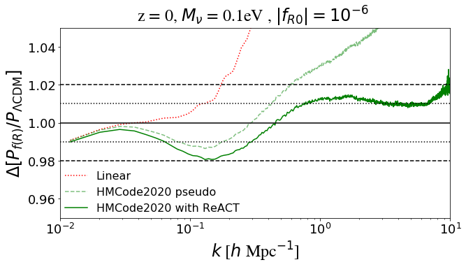
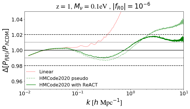
Figure 1: Comparison of theoretical predictions to DUSTGRAIN-pathfinder measurements in $f(R)$ + $M_{\nu}$ (case (a) in main text) with $|f_{\rm R0}|=10^{-6}$ and $M_{\nu}=0.1$eV. We compare the ratio of the $f(R)$ + $M_{\nu}$ $P(k)$ to the $\Lambda$CDM $P(k)$, in the two cases. Top is $z=0$ and bottom is $z=1$. We show linear (red dotted), HMCode2020 pseudo (green dashed) and HMCode2020 pseudo with reaction (green solid) predictions.

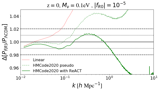
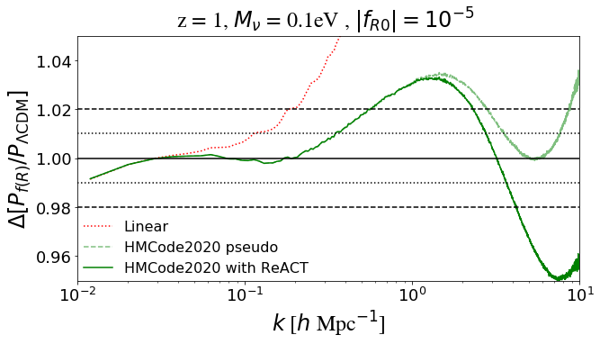
Figure 2: Comparison of theoretical predictions to DUSTGRAIN-pathfinder measurements in $f(R)$ + $M_{\nu}$ (case (b) in main text) with $|f_{\rm R0}|=10^{-5}$ and $M_{\nu}=0.1$eV. We compare the ratio of the $f(R)$ + $M_{\nu}$ $P(k)$ to the $\Lambda$CDM $P(k)$, in the two cases. Top is $z=0$ and bottom is $z=1$. We show linear (red dotted), HMCode2020 pseudo (green dashed) and HMCode2020 pseudo with reaction (green solid) predictions.

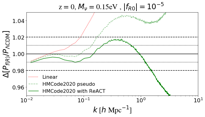
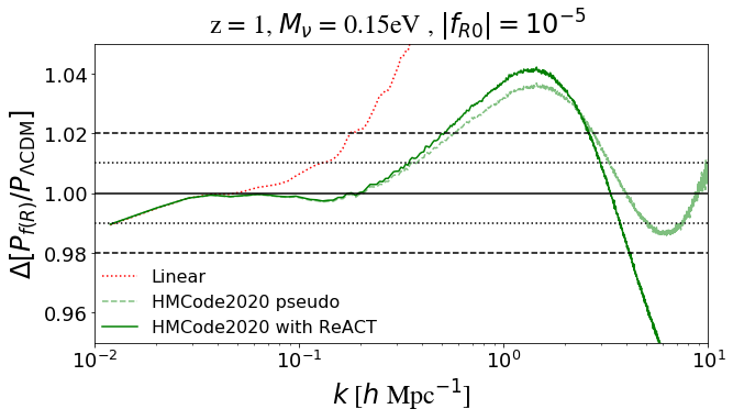
Figure 3: Comparison of theoretical predictions to DUSTGRAIN-pathfinder measurements in $f(R)$ + $M_{\nu}$ (case (c) in main text) with $|f_{\rm R0}|=10^{-5}$ and $M_{\nu}=0.15$eV. We compare the ratio of the $f(R)$ + $M_{\nu}$ $P(k)$ to the $\Lambda$CDM $P(k)$, in the two cases. Top is $z=0$ and bottom is $z=1$. We show linear (red dotted), HMCode2020 pseudo (green dashed) and HMCode2020 pseudo with reaction (green solid) predictions.

3.1.2 $w$CDM with massive neutrinos

For this scenario we will compare the predictions of Equation 1 with predictions given by the Bacco emulator (Angulo et al., 2020) and the EuclidEmulator2 (Euclid Collaboration et al., 2020). The Bacco (EuclidEmulator2) is expected to be accurate at the $3(\leq 1)\%$ level down to $k=5(10)h$/Mpc.

We adopt the base cosmology $h=0.7$, $n_{s}=0.972$, $\Omega_{m}=0.2793$ and $\Omega_{b}=0.0463$. We then take 6 samples from the overlapping parameter space of both emulators in $\{M_{\nu},w_{0},w_{a}\}\in\{[0,0.15]eV,[-1.15,-0.85],[-0.3,0.3]\}$. For these 6 cosmologies, we compare the EuclidEmulator2 emulator predictions with the Bacco emulator, the Halofit fitting formula (Takahashi et al., 2012), the stand-alone HMCode2020 predictions and finally with Equation 1 (a non-linear pseudo spectrum given by HMCode2020 combined with the halo model reaction given in Equation 2).

We show the ratios of the various prescriptions for $P_{\rm NL}(k)$ to the EuclidEmulator2 in Figure 4. We find that an HMCode2020 prescription for the pseudo spectrum combined with the halo model reaction offers 1(2)% consistency with EuclidEmulator2 at $z=1(0)$ for $k\leq 1h/{\rm Mpc}$ for the full range of $\nu w$CDM cosmologies considered. The accuracy remains at the $2\%$ level down to $k=5h/{\rm Mpc}$ at z=0 for all cosmologies but worsens to the $5\%$ level for large values of $|w_{a}|$ at $z=1$.

The accuracy of our approach is comparable to HMCode2020’s $\nu w$CDM predictions over the full range of cosmologies while Bacco deviates largely for large modifications to a constant dark energy which is consistent with the results shown in Appendix A of Contreras et al. (2020). Halofit on the other hand shows up to 5% disagreement for all cosmologies beyond $k\approx 0.5h/{\rm Mpc}$.

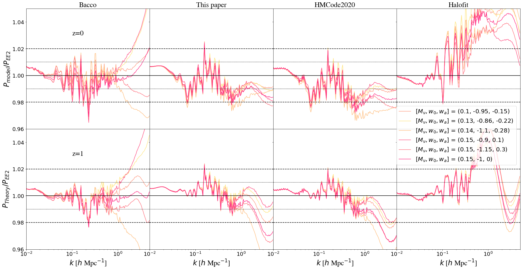
Figure 4: Each column shows the ratio of a particular prescription for the non-linear matter power spectrum to the EuclidEmulator2 prediction. The various lines represent cosmologies with a different choice of sum of neutrino mass $M_{\rm\nu}$ and dark energy equation of state parameters $\{w_{0},w_{a}\}$. Top panels show the results for $z=0$ and bottom panels for $z=1$.

To further test the limitations of our modelling prescription, we have also investigated some extreme parameter choices which are well beyond the current cosmological constraints (see for example Aghanim et al. (2020)). These are shown in Figure 5. We consider two large neutrino mass cases which are permitted by the Bacco emulator range and two large deviations from a constant dark energy permitted by the Euclid emulator range. For most cases we find Equation 1 remains within $2\%$ of the emulators down to $k=1h/{\rm Mpc}$ at $z=0$ and $z=1$ with the exception of a case with $w_{a}=0.5$ which is at the edge of the range at which the current version of ReACT is numerically stable ($w_{a}\leq 0.8$). This case deviates by more than $2\%$ from EuclidEmulator2 at $k\approx 0.3h/{\rm Mpc}$. Again HMCode2020 shows similar consistency with the emulators in this range overall while halofit disagrees with the emulators beyond 5% above $k\approx 5h/{\rm Mpc}$.

In all cases considered we note that the reaction adds significant accuracy to the HMCode2020 pseudo spectrum, especially above $k=1h$/Mpc.

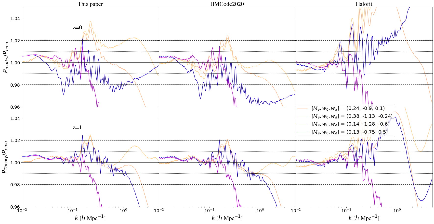
Figure 5: ‘Extreme’ cases: Each column shows the ratio of a particular prescription for the non-linear matter power spectrum to an emulator prediction. In particular, the orange curves are compared to the Bacco emulator while the purple curves to the EuclidEmulator2. The various lines represent cosmologies with a different choice of sum of neutrino mass $M_{\rm\nu}$ and dark energy equation of state parameters $\{w_{0},w_{a}\}$. Top panels show the results for $z=0$ and bottom panels for $z=1$.

3.2 Including baryonic feedback

We now look to include baryonic effects in our predictions. To do this we make use of the feedback modelling included in HMCode2020. We compare to the BAHAMAS suite of cosmological hydrodynamical simulations (McCarthy et al., 2017; McCarthy et al., 2018). In particular we will make use of the $\nu\Lambda$CDM and $\nu w$CDM BAHAMAS simulations described in van Daalen et al. (2020) and Pfeifer et al. (2020) respectively. The HMCode2020 feedback parameter is set to $\log_{10}(T_{\rm AGN}/K)=7.8$ which was fit to the $\nu\Lambda$CDM BAHAMAS simulations (Mead et al., 2021).

The effects of feedback from AGN and stellar sources (supernovae) are incorporated in the BAHAMAS simulations using subgrid models that have a number of free parameters. As described in McCarthy et al. (2017), these parameters were adjusted so that the simulations reproduce the local galaxy stellar mass function and the hot gas mass fractions of galaxy groups and clusters, thus ensuring that massive haloes (which contribute the most to the matter power spectrum) have the correct baryon fractions. Note that van Daalen et al. (2020) have shown that having the correct baryon fractions is key to obtaining a realistic impact of baryons on the total matter power spectrum. Furthermore, both McCarthy et al. (2018) and van Daalen et al. (2020) have shown that the impact of baryons on the power spectrum is only very weakly dependent on cosmology (primarily through the universal baryon fraction, $\Omega_{b}/\Omega_{m}$), such that recalibration of the feedback is generally unnecessary when varying cosmology. Indeed, for the $\nu\Lambda$CDM and $\nu w$CDM simulations we use here, the feedback prescription was left unchanged from the fiducial BAHAMAS run but it was verified that the relative impact of the power spectrum (or the predicted baryon fractions) did not change by more than about a percent. Finally, we note that van Daalen et al. (2020) have demonstrated that on very large scales (where the impact of baryons is expected to be unimportant) the ratio of the hydro simulations to their dissipationless counterparts converges to typically better than 0.1% accuracy, which might be viewed as the numerical accuracy of the predicted (relative) power spectra.

3.2.1 $\nu\Lambda$CDM

We consider the WMAP9 cosmology of this suite which adopts the baseline parameters $h=0.7$, $n_{s}=0.972$, $\Omega_{m}=0.2793$, $\Omega_{b}=0.0463$ and $A_{s}=2.392\times 10^{-9}$. We consider 3 massive neutrino cases:

1. Low mass: $M_{\nu}=0.06$eV ($\Omega_{\nu}=0.0013$, $\Omega_{\rm cdm}=0.2317$).

2. Medium mass: $M_{\nu}=0.24$eV ($\Omega_{\nu}=0.0053$, $\Omega_{\rm cdm}=0.2277$).

3. High mass: $M_{\nu}=0.48$eV ($\Omega_{\nu}=0.0105$, $\Omega_{\rm cdm}=0.2225$).

We again show the ratio of the quantity $P_{\rm mnu+b}(k)/P_{\Lambda{\rm CDM}}$, where ‘mnu+b’ stands for the massive neutrino cosmology with baryonic effects, between the theoretical predictions and the simulation measurements. This is shown for cases (a), (b) and (c) in Figure 6, Figure 7 and Figure 8 respectively. For all cases we find that the halo model reaction combined with the HMCode2020 pseudo spectrum is $\leq 3\%$ accurate for $k\leq 5h/{\rm Mpc}$ for $z=0$ and $z=1$, with the predictions generally being more accurate for lower neutrino mass and $z=0$. Further, for all cases we find sub-percent agreement over all scales and redshifts between the stand-alone HMCode2020 and the halo model reaction with a pseudo HMCode2020 prediction. We note that the feedback model of HMCode2020 is fit to the BAHAMAS simulations and so the high degree of accuracy is not surprising.

It is worth highlighting that the baryonic feedback model of HMCode2020 is implemented through another ‘reaction’, that of the dark matter spectrum to baryonic effects. Thus, our predictions are applying two reactions independently: one for massive neutrinos and one for baryonic effects, both based on different conventions. Ideally, these would be combined consistently into a single reaction as we have done for massive neutrinos and modified gravity or dark energy. We leave this for future work. This being said, the results of Mead et al. (2016b) show a high degree of independence between massive neutrino and baryonic effects down to $k=10h/{\rm Mpc}$ which is consistent with both the accuracy found in Figure 6, Figure 7 and Figure 8, as well as the consistency between the single reaction application of HMCode2020 (cyan curves) and the double-reaction application HMCode2020-pseudo together with the massive neutrino reaction.

Again, we also note the tilt (and non-unity ratio) observed in the comparisons at large scales are likely due to relativistic effects included in the linear power spectrum produced by MGCAMB, as also noted in the DUSTGRAIN-pathfinder simulation comparisons.

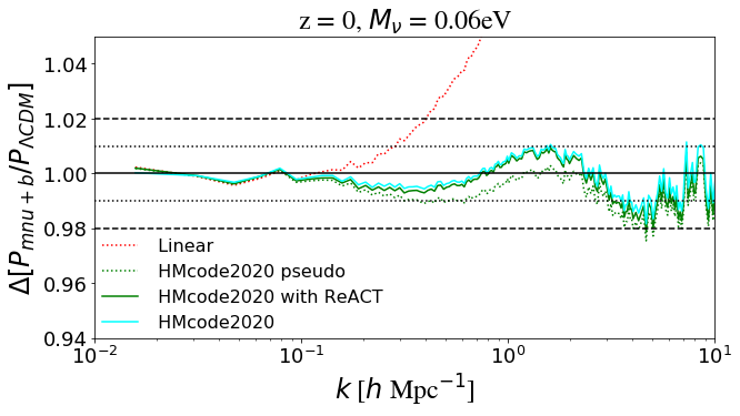
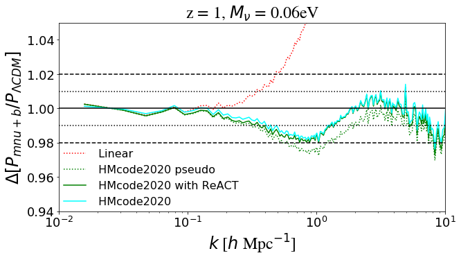
Figure 6: Comparison of theoretical predictions to BAHAMAS measurements in $\nu\Lambda$CDM (case (a) in main text) with $M_{\nu}=0.06$eV. We compare the ratio of the $\nu\Lambda$CDM $P(k)$ to the $\Lambda$CDM $P(k)$, in the two cases. Top is $z=0$ and bottom is $z=1$. We show linear (red dotted), HMCode2020 pseudo (green dashed), HMCode2020 pseudo with reaction (green solid) and HMCode2020 (cyan solid) predictions.

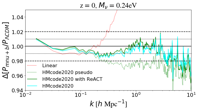
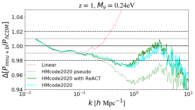
Figure 7: Comparison of theoretical predictions to BAHAMAS measurements in $\nu\Lambda$CDM (case (b) in main text) with $M_{\nu}=0.24$eV. We compare the ratio of the $\nu\Lambda$CDM $P(k)$ to the $\Lambda$CDM $P(k)$, in the two cases. Top is $z=0$ and bottom is $z=1$. We show linear (red dotted), HMCode2020 pseudo (green dashed), HMCode2020 pseudo with reaction (green solid) and HMCode2020 (cyan solid) predictions.

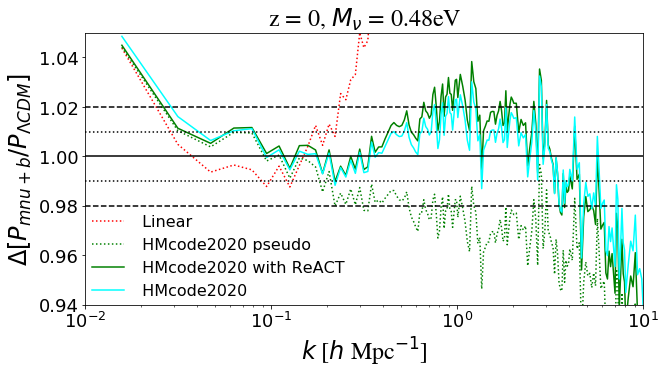
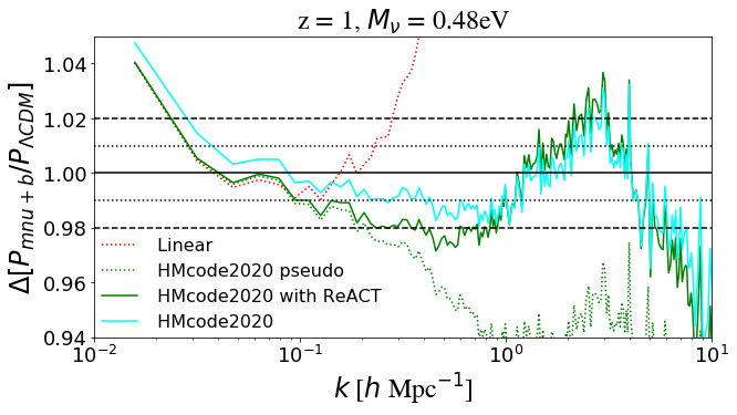
Figure 8: Comparison of theoretical predictions to BAHAMAS measurements in $\nu\Lambda$CDM (case (c) in main text) with $M_{\nu}=0.48$eV. We compare the ratio of the $\nu\Lambda$CDM $P(k)$ to the $\Lambda$CDM $P(k)$, in the two cases. Top is $z=0$ and bottom is $z=1$. We show linear (red dotted), HMCode2020 pseudo (green dashed), HMCode2020 pseudo with reaction (green solid) and HMCode2020 (cyan solid) predictions.

3.2.2 $\nu w$CDM

We will make use of three simulations from this suite, all of which have $n_{s}=0.97$ and a neutrino mass of $M_{\nu}=0.06$eV. The other cosmological parameters are detailed below:

1. Non-phantom: $\Omega_{m}=0.286$, $\Omega_{b}=0.0462$, $H_{0}=69.97$, $\sigma_{8}=0.819$ and $\{w_{0},w_{a}\}=\{-0.67,-1.45\}$.

2. Phantom: $\Omega_{m}=0.309$, $\Omega_{b}=0.0501$, $H_{0}=67.25$, $\sigma_{8}=0.773$ and $\{w_{0},w_{a}\}=\{-1.16,0.73\}$.

3. $\nu\Lambda$CDM: $\Omega_{m}=0.294$, $\Omega_{b}=0.0476$, $H_{0}=68.98$ and $\sigma_{8}=0.802$ (dark matter only).

In this subsection the theoretical predictions for cases (a) and (b) follow Equation 1 with $\mathcal{R}$ including both evolving dark energy and massive neutrino effects while $P^{\rm pseudo}_{\rm NL}$ again includes baryonic feedback effects. Case (c) will also follow Equation 1 but $\mathcal{R}$ will only model the effect of a non-zero neutrino mass and $P^{\rm pseudo}_{\rm NL}$ will include no baryonic feedback effects. We again show the stand-alone HMCode2020 predictions too which supports $\nu w$CDM cosmologies.

We note that the simulation measurements in these cases are of the cold dark matter plus baryon (cb) power spectrum and do not include the massive neutrino contribution directly. The theoretical predictions have been adjusted accordingly. We have checked that for the ratios we plot, the theoretical predictions for the full matter spectrum and for the cb spectrum are almost identical.

The ratio of cases (a) and (b) to case (c) as given by theory to the same ratio as measured from the simulations are shown in Figure 9 and Figure 10 respectively. For both cases we find that the halo model reaction combined with a HMCode2020 pseudo is $\leq 2\%$ accurate for $k\leq 5h/{\rm Mpc}$ for $z=0$ and $z=1$. As in the $\nu\Lambda$CDM cases shown in subsubsection 3.2.1, the predictions of Equation 1 are generally in sub-percent agreement with the stand-alone HMCode2020 predictions.

The lack of a $\Lambda$CDM simulation without massive neutrinos nor higher neutrino mass $\nu w$CDM simulations prevents us from investigating the accuracy of our combined massive neutrino and evolving dark energy theoretical prescription in more detail. We do however find that the accuracy demonstrated for these two cases is shown for all the $\nu w$CDM cosmologies outlined in Pfeifer et al. (2020), with the inclusion of the reaction $\mathcal{R}$ generally adding to the accuracy of Equation 1. Further, this supports the reliability of modelling evolving dark energy and baryonic effects independently.

Finally, we note that the magnitude and shape of the reaction in our calculations inferred from Figure 9 is very similar to what was found in C19. In particular their DE5 case is very similar to our case (a), exhibiting a $2\%$ accuracy with their dark matter simulations up to $k\sim 5h/{\rm Mpc}$. This further indicates that the small neutrino mass, baryonic effects and variation in cosmology within the ratio of our cases (a), (b) and (c) has minimal effect.

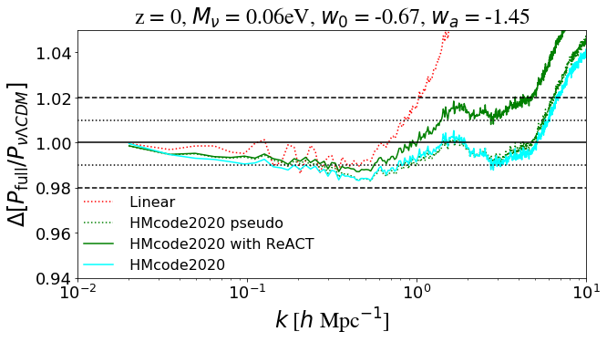
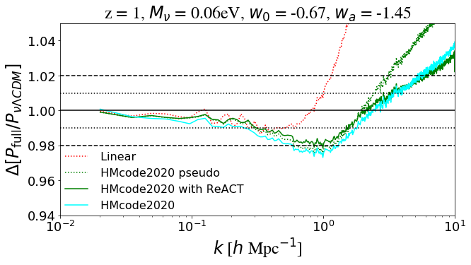
Figure 9: Comparison of theoretical predictions to BAHAMAS measurements in non-phantom $\nu w$CDM (case (a) in main text) with $M_{\nu}=0.06$eV. We compare the ratio of the $\nu w$CDM $P(k)$ to the $\nu\Lambda$CDM $P(k)$, in the two cases. Top is $z=0$ and bottom is $z=1$. We show linear (red dotted), HMCode2020 pseudo (green dashed), HMCode2020 pseudo with reaction (green solid) and HMCode2020 (cyan solid) predictions.

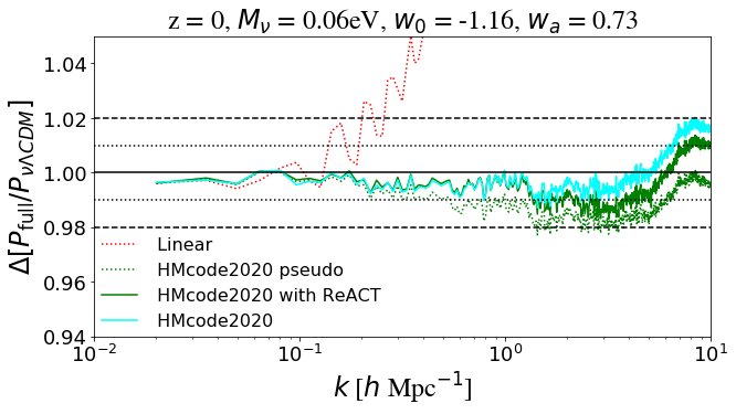
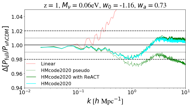
Figure 10: Comparison of theoretical predictions to BAHAMAS measurements in phantom $\nu w$CDM (case (b) in main text) with $M_{\nu}=0.06$eV. We compare the ratio of the $\nu w$CDM $P(k)$ to the $\nu\Lambda$CDM $P(k)$, in the two cases. Top is $z=0$ and bottom is $z=1$. We show linear (red dotted), HMCode2020 pseudo (green dashed), HMCode2020 pseudo with reaction (green solid) and HMCode2020 (cyan solid) predictions.

4 Summary

In this paper we have combined the halo model reaction for modified gravity and non-constant dark energy (Cataneo et al., 2019) with the halo model reaction for massive neutrinos (Cataneo et al., 2020). Combined with a baryonic feedback model and an accurate pseudo spectrum prescription, this offers an analytic means to model theoretically general matter power spectra in the non-linear regime of structure formation at percent level accuracy. We have implemented this extension into the ReACT code (Bose et al., 2020).

We have tested the halo model reaction applied to a pseudo spectrum given by the halo model-based prescription of Mead et al. (2021) (HMCode2020) against the DUSTGRAIN-pathfinder simulations (Giocoli et al., 2018), the BAHAMAS hydrodynamical simulations (McCarthy et al., 2017; Pfeifer et al., 2020), the Bacco emulator (Angulo et al., 2020) and the official Euclid emulator (Euclid Collaboration et al., 2020). Our results are summarised in Table 1.

We find that the theoretical model is generally applicable at the $3\%$-accuracy level for $k\leq 1h/{\rm Mpc}$ for $M_{\nu}\leq 0.15$eV, $|f_{\rm R0}|\leq 10^{-5}$ and observationally-permitted values of $\{w_{0},w_{a}\}$ (see Pfeifer et al. (2020)). Tests with more accurate pseudo prescriptions, such as COmoving Lagrangian Acceleration (COLA) simulations, show that most of the inaccuracy over this range of scales comes from the HMCode2020 pseudo spectrum prescription. This was also shown in C19. Improvements to the non-linear pseudo power spectrum are thus essential for achieving the theoretical accuracy requirements of upcoming surveys such as Euclid.

For low neutrino masses ($M_{\nu}\leq 0.1$eV) and low deviations to $\Lambda$CDM (e.g. for an $f(R)$ modification, $|f_{\rm R0}|\leq 10^{-6}$), the halo model reaction and HMCode2020 can be reliably applied at $2\%$ accuracy at scales $k\leq 3h/{\rm Mpc}$. Further, we have also found that evolving dark energy and massive neutrino effects can be reliably modelled independently of baryonic feedback effects, although we aim to test the consistent combination of these effects in future work. This is consistent with the work of Mummery et al. (2017) and Pfeifer et al. (2020) which shows that baryonic effects on the matter power spectrum can be treated independently of the effects of massive neutrinos and evolving dark energy down to an accuracy of $\leq 2\%$ and $\leq 1\%$, respectively. The accuracy of the model proposed in this paper is in superb agreement with current state-of-the-art prescriptions for $\nu w$CDM cosmologies, particularly HMCode2020, with the advantage of offering greater model generality and clear pathways for improvement in accuracy.

On this point, the combination of HMCode2020 and ReACT offers a very competitive framework to constrain $\nu w$CDM cosmologies as well as modified gravity, using say cosmic shear data. It can also be used to extend the recent neural network BaCoN (Mancarella et al., 2020) to distinguish between non-zero neutrino masses and modified cosmologies and gravity. The modelling of modified gravity theories with scale-dependent growth and massive neutrinos is slightly more restrictive in the scales that it can be reliably applied to. We expect theories with scale-independent growth, such as the DGP braneworld model (Dvali et al., 2000), to be better modelled by this framework when also including massive neutrinos (see C19 for example).

Table 1: Maximal percent deviation of the halo model reaction with HMCode2020 against various benchmarks at different scales when comparing the ratio of the target spectrum to a $\Lambda$CDM spectrum. We show the percent deviation from the benchmark at $z=0$ and $z=1$. We have considered $0.06$eV $\leq M_{\nu}\leq 0.48$eV, $|f_{\rm R0}|\leq 10^{-5}$ and a broad range of $\{w_{0},w_{a}\}$. EE2 stands for EuclidEmulator2. For the emulator accuracies, we do not consider the ‘extreme’ cases shown in Figure 5.

	$k\leq 1h/{\rm Mpc}$		$k\leq 3h/{\rm Mpc}$
Benchmark	z=0	z=1	z=0	z=1
$f(R)+M_{\nu}$ (DUSTGRAIN-pathfinder)	2%	3%	5%	4%
$\nu\Lambda$CDM (BAHAMAS)	2%	2%	2%	2%
$\nu w$CDM (EE2)	2%	1%	2%	4%
$\nu w$CDM (Bacco)	2%	1%	2%	4%
$\nu w$CDM (BAHAMAS)	2%	2%	2%	2%

As stated, the main source of inaccuracy for scales $k\leq 3h/{\rm Mpc}$ is the HMCode2020 pseudo power spectrum prescription.This limiting accuracy is confirmed in our comparisons where we observe sub-percent agreement between the halo model reaction approach and the ‘pure’ HMCode2020 predictions for all $\nu w$CDM cosmologies considered. Further inaccuracy in our approach comes from ill-calibrated mass functions in both pseudo and target cosmologies as well as inaccurate concentration-mass relations. This was also shown in Srinivasan et al. (2021) where they were able to significantly improve the theoretical accuracy by tuning the halo concentration-mass relation within the halo model reaction. Similarly in C19, they show the benefit of using the ‘correct’ $c$-$M$ relation. In Figure 11 we illustrate the ideal setup for the non-linear power spectrum predictions under this framework. The pseudo spectrum is given by a bespoke emulator as proposed in Giblin et al. (2019), as are the ($\Lambda$CDM based) pseudo spherical collapse quantities. The real spherical collapse quantities are parametrised and constrained by astronomical observations, such as cluster abundance data. The real halo density profile used in the reaction can also be constrained by data such as total matter profiles, which would also give a self-consistent model for baryonic effects.

In future work we aim to integrate the massive neutrino section of the code into CosmoSIS (Zuntz et al., 2015) and perform Markov Chain Monte Carlo analyses on the measured cosmic shear spectrum from beyond-$\Lambda$CDM simulations to set clear scale cuts on the framework as well as forecasts for upcoming surveys. We also aim at testing the independency of baryonic effects and modified gravity/dark energy/massive neutrinos. As mentioned above, some work in this direction has been carried out by Mummery et al. (2017) and Pfeifer et al. (2020) (for massive neutrino and DE cosmologies), and by Arnold & Li (2019) (for $f(R)$ gravity). Most likely Vainshtein screening is highly effective at screening halos, so one would expect almost perfect decoupling between baryonic feedback and MG physics.

We are also currently working on generalising the parametrisation of modified gravity and dark energy within the halo model reaction. This could then be validated against parametrised $N$-body simulations which have seen significant development recently (Hassani & Lombriser, 2020; Srinivasan et al., 2021).

Figure 11: An idealised pipeline for the non-linear power spectrum (green trapezium) computation. Data sets (orange trapezium), such as cluster abundances, directly constrain the real halo mass function (cyan rectangle) while a suite of $\Lambda$CDM based simulations (yellow trapezium) provide emulated pseudo halo model ingredients (red rectangle) (we exclude the density profile since NFW works sufficiently well). These same simulations are used to construct the pseudo non-linear power spectrum (gray rectangle). The halo model ingredients are provided to a code such as ReACT to compute the halo model reaction (blue rectangle). Standard plus the extended cosmological parameters describing beyond-$\Lambda$CDM physics (including neutrino mass) are supplied to both the emulated quantities as well as the reaction computation. The baryonic feedback effects are ideally self consistently included in the halo model through $\rho^{\rm real}_{\rm DM,gas,stars}$ constrained by total matter profiles, or can be optionally added onto $P_{\rm NL}^{\rm pseudo}$ separately through some feedback model (beige trapezium).

Data Availability

The software used in this article is publicly available in the ReACT repository at https://github.com/nebblu/ReACT/tree/react_with_neutrinos. The BAHAMAS simulation data used in this work is publicly available at http://powerlib.strw.leidenuniv.nl/#data.

Appendix A Simulating the pseudo spectrum with COLA in $f(R)$ gravity with massive neutrinos

Here we check the accuracy of the HMCode2020 prescription for the non-linear pseudo power spectrum by running a set of COmoving Lagrangian Acceleration (COLA) simulations in $f(R)$ gravity with massive neutrinos using the approach from Winther et al. (2017) and Wright et al. (2017) that is implemented in the publicly available COLA code FML. These are approximate simulation methods that make use of 2nd order Lagrangian perturbation theory to trade accuracy on small scales for faster speed overall, while keeping accuracy on large scales. We note that due to the approximate nature of these COLA simulations, we do not expect their pseudo spectra, which are essentially a $\Lambda$CDM simulation with modified initial conditions, to match the accuracy of those from HMCode2020 which is fit to full $N$-body simulations, for $k\gtrsim 1h/{\rm Mpc}$ at $z=0$. We have selected the medium and high deviation from $\Lambda$CDM cases, (b) and (c), described in subsubsection 3.1.1, so $|f_{\rm R0}|=10^{-5}$ and $M_{\nu}=0.1$eV (b) and $M_{\nu}=0.15$eV (c).

We show the results in Figure 12 and Figure 13. The gray triangles show the ratio of ratios between the two COLA simulation measurements of the power spectrum, in the modified cosmology and $\Lambda$CDM, to the same ratio for the DUSTGRAIN-pathfinder $N$-body simulations. This gives an indication of the overall accuracy of the COLA approach. For $M_{\nu}=0.1(0.15)$eV we find that, at $z=1$, the reaction given in Equation 2 combined with a COLA measured pseudo spectrum is at least $2(3)\%$ accurate at scales $k\leq 3h/{\rm Mpc}$. For both cases, at $z=0$ the $2\%$ accuracy-level of the COLA pseudo with the halo model reaction is guaranteed for scales less than $k\approx 1h/{\rm Mpc}$, which is roughly the same accuracy as the ratio of the full COLA simulations when compared to DUSTGRAIN-pathfinder.

Importantly, these comparisons indicate that a significant part of the inaccuracies seen at $z=1$ at $k\leq 3h/{\rm Mpc}$ for the medium (b) and high (c) deviation cases (see Figure 2 and Figure 3) come from the HMCode2020 pseudo spectrum. We note that further discrepancies, specifically in the $M_{\nu}=0.15$eV case, come from using inaccurate mass function fits in the 1-halo terms. This is indicated by the enhancement of power the reaction gives the pseudo spectrum (see dotted and solid green lines in the bottom plot of Figure 3). It is in this case that we get $1<\mathcal{E}\sim P_{\rm 1h}^{\rm cb}/P_{\rm 1h}^{\rm pseudo}$ which produces this enhancement (see Equation 2 and Equation 4). This is highlighted in Figure 14 where we plot the 1-loop perturbation theory prediction for the reaction (see Equation 13), the halo model reaction and the measurement from COLA for $z=1$ in both cases (b) and (c). We clearly see an over-estimation of the halo model reaction at quasi non-linear scales indicating that $\mathcal{E}$ should be less than 1. Note that in these cases we find no solution for $k_{\star}$ and so $\mathcal{E}$ is set to unity . We expect this source of inaccuracy to be remedied by measuring the mass function directly from simulations or constraining it using data.

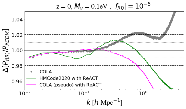
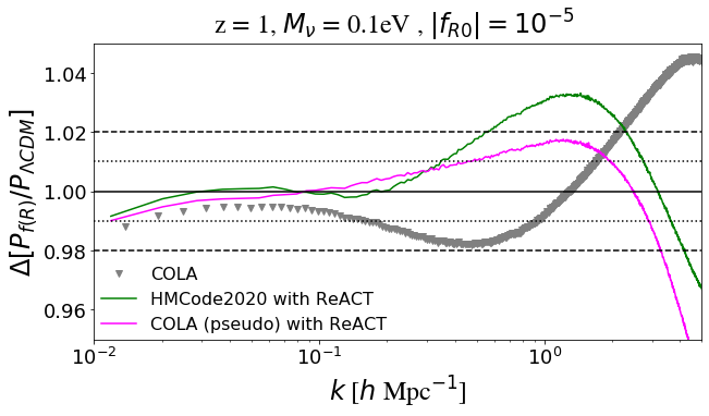
Figure 12: Ratio of theoretical predictions to DUSTGRAIN-pathfinder measurement of the $f(R)$ to the (massless neutrino) $\Lambda$CDM $P(k)$ ratio with $|f_{\rm R0}|=10^{-5}$ and $M_{\nu}=0.1$eV. Top is $z=0$ and bottom is $z=1$. We show the full COLA measurements (gray triangles), the HMCode2020 pseudo with reaction (green solid) predictions and the COLA pseudo with reaction (magenta solid) predictions.

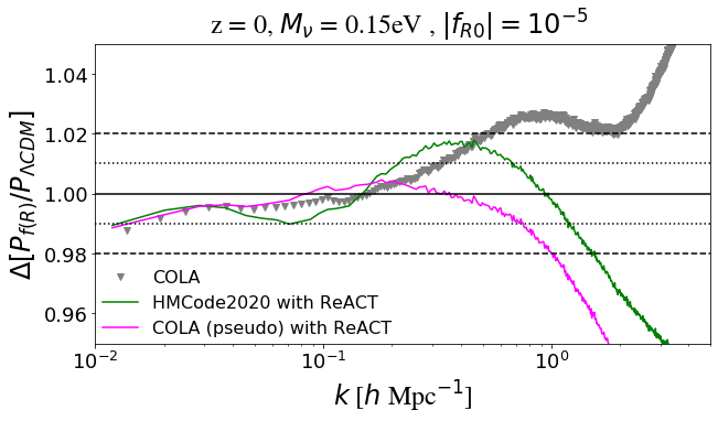
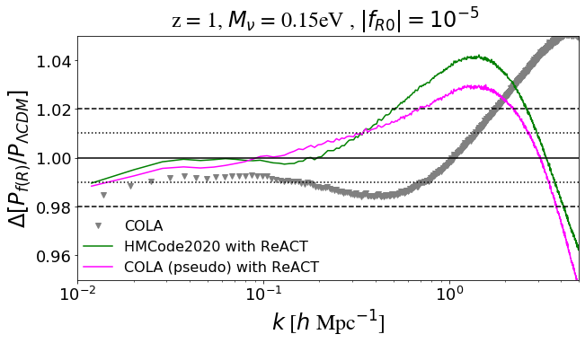
Figure 13: Ratio of theoretical predictions to DUSTGRAIN-pathfinder measurement of the $f(R)$ to the (massless neutrino) $\Lambda$CDM $P(k)$ ratio with $|f_{\rm R0}|=10^{-5}$ and $M_{\nu}=0.15$eV. Top is $z=0$ and bottom is $z=1$. We show the full COLA measurements (gray triangles), the HMCode2020 pseudo with reaction (green solid) predictions and the COLA pseudo with reaction (magenta solid) predictions.

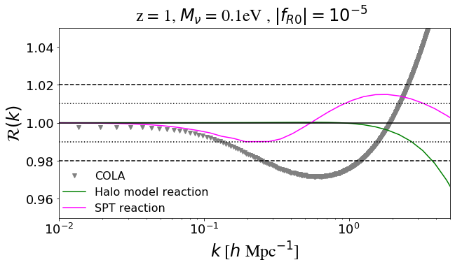
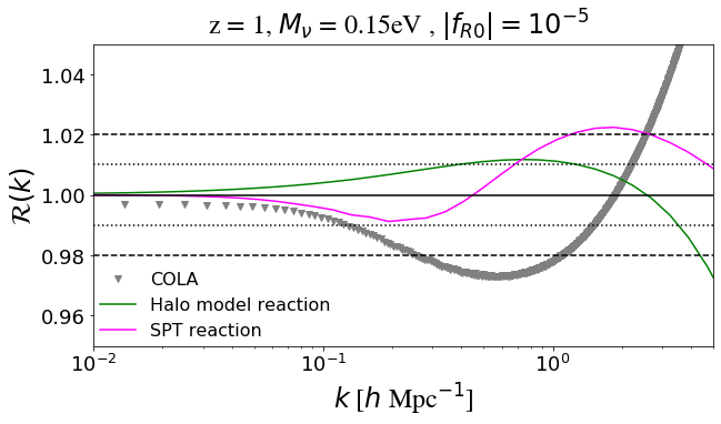
Figure 14: The matter power spectrum reaction as measured from COLA (gray triangles), the halo model reaction prediction (green solid) and the 1-loop perturbation theory prediction (magenta solid) at $z=1$ for cases (b) (top panel) and (c) (bottom panel).

References

- Abbott et al. (2020) Abbott T. M. C., et al., 2020, Phys. Rev. D, 102, 023509
- Agarwal & Feldman (2011) Agarwal S., Feldman H. A., 2011, Mon. Not. Roy. Astron. Soc., 410, 1647
- Aghanim et al. (2020) Aghanim N., et al., 2020, Astron. Astrophys., 641, A6
- Akeson et al. (2019) Akeson R., et al., 2019, arXiv e-prints, p. arXiv:1902.05569
- Amendola et al. (2018) Amendola L., et al., 2018, Living Rev. Rel., 21, 2
- Anderson et al. (2013) Anderson L., et al., 2013, Mon. Not. Roy. Astron. Soc., 427, 3435
- Angulo et al. (2020) Angulo R. E., Zennaro M., Contreras S., Aricò G., Pellejero-Ibañez M., Stücker J., 2020, arXiv e-prints, p. arXiv:2004.06245
- Aricò et al. (2020) Aricò G., Angulo R. E., Contreras S., Ondaro-Mallea L., Pellejero-Ibañez M., Zennaro M., 2020, arXiv e-prints, p. arXiv:2011.15018
- Arnold & Li (2019) Arnold C., Li B., 2019, MNRAS, 490, 2507
- Beutler et al. (2017) Beutler F., et al., 2017, Mon. Not. Roy. Astron. Soc., 466, 2242
- Bird et al. (2012) Bird S., Viel M., Haehnelt M. G., 2012, MNRAS, 420, 2551
- Bird et al. (2018) Bird S., Ali-Haïmoud Y., Feng Y., Liu J., 2018, MNRAS, 481, 1486
- Blanchard et al. (2020) Blanchard A., et al., 2020, Astron. Astrophys., 642, A191
- Blas et al. (2014) Blas D., Garny M., Konstandin T., Lesgourgues J., 2014, J. Cosmology Astropart. Phys., 2014, 039
- Bose & Koyama (2016) Bose B., Koyama K., 2016, JCAP, 1608, 032
- Bose et al. (2020) Bose B., Cataneo M., Tröster T., Xia Q., Heymans C., Lombriser L., 2020, Mon. Not. Roy. Astron. Soc., 498, 4650
- Boyle et al. (2020) Boyle A., Uhlemann C., Friedrich O., Barthelemy A., Codis S., Bernardeau F., Giocoli C., Baldi M., 2020, arXiv e-prints, p. arXiv:2012.07771
- Bullock et al. (2001) Bullock J. S., Kolatt T. S., Sigad Y., Somerville R. S., Kravtsov A. V., Klypin A. A., Primack J. R., Dekel A., 2001, Mon. Not. Roy. Astron. Soc., 321, 559
- Cacciato et al. (2009) Cacciato M., Bosch F. C. v. d., More S., Li R., Mo H. J., Yang X., 2009, Mon. Not. Roy. Astron. Soc., 394, 929
- Cataneo et al. (2019) Cataneo M., Lombriser L., Heymans C., Mead A., Barreira A., Bose S., Li B., 2019, Mon. Not. Roy. Astron. Soc., 488, 2121
- Cataneo et al. (2020) Cataneo M., Emberson J., Inman D., Harnois-Deraps J., Heymans C., 2020, Mon. Not. Roy. Astron. Soc., 491, 3101
- Chevallier & Polarski (2001) Chevallier M., Polarski D., 2001, Int. J. Mod. Phys., D10, 213
- Chisari et al. (2019) Chisari N. E., et al., 2019, Open J. Astrophys., 2, 4
- Clifton et al. (2012) Clifton T., Ferreira P. G., Padilla A., Skordis C., 2012, Phys. Rept., 513, 1
- Contarini et al. (2021) Contarini S., Marulli F., Moscardini L., Veropalumbo A., Giocoli C., Baldi M., 2021, MNRAS,
- Contreras et al. (2020) Contreras S., Angulo R. E., Zennaro M., Aricò G., Pellejero-Ibañez M., 2020, Mon. Not. Roy. Astron. Soc., 499, 4905
- Cooray & Sheth (2002) Cooray A., Sheth R. K., 2002, Phys. Rept., 372, 1
- Copeland et al. (2006) Copeland E. J., Sami M., Tsujikawa S., 2006, Int. J. Mod. Phys., D15, 1753
- Corasaniti et al. (2020) Corasaniti P. S., Giocoli C., Baldi M., 2020, Phys. Rev. D, 102, 043501
- Costanzi et al. (2013) Costanzi M., Villaescusa-Navarro F., Viel M., Xia J.-Q., Borgani S., Castorina E., Sefusatti E., 2013, J. Cosmology Astropart. Phys., 2013, 012
- DeRose et al. (2019) DeRose J., et al., 2019, ApJ, 875, 69
- Dolag et al. (2004) Dolag K., Bartelmann M., Perrotta F., Baccigalupi C., Moscardini L., Meneghetti M., Tormen G., 2004, Astron. Astrophys., 416, 853
- Dvali et al. (2000) Dvali G., Gabadadze G., Porrati M., 2000, Phys.Lett., B485, 208
- Euclid Collaboration et al. (2020) Euclid Collaboration et al., 2020, arXiv e-prints, p. arXiv:2010.11288
- Ferreira (2019) Ferreira P. G., 2019, Ann. Rev. Astron. Astrophys., 57, 335
- García-Farieta et al. (2019) García-Farieta J. E., Marulli F., Veropalumbo A., Moscardini L., Casas-Miranda R. A., Giocoli C., Baldi M., 2019, MNRAS, 488, 1987
- Giblin et al. (2019) Giblin B., Cataneo M., Moews B., Heymans C., 2019, Mon. Not. Roy. Astron. Soc., 490, 4826
- Giocoli et al. (2010) Giocoli C., Bartelmann M., Sheth R. K., Cacciato M., 2010, Mon. Not. Roy. Astron. Soc., 408, 300
- Giocoli et al. (2015) Giocoli C., Metcalf R. B., Baldi M., Meneghetti M., Moscardini L., Petkova M., 2015, MNRAS, 452, 2757
- Giocoli et al. (2018) Giocoli C., Baldi M., Moscardini L., 2018, Mon. Not. Roy. Astron. Soc., 481, 2813
- Girelli et al. (2020) Girelli G., Pozzetti L., Bolzonella M., Giocoli C., Marulli F., Baldi M., 2020, A&A, 634, A135
- Hagstotz et al. (2019) Hagstotz S., Costanzi M., Baldi M., Weller J., 2019, MNRAS, 486, 3927
- Hassani & Lombriser (2020) Hassani F., Lombriser L., 2020, Mon. Not. Roy. Astron. Soc., 497, 1885
- Heymans et al. (2021) Heymans C., et al., 2021, A&A, 646, A140
- Hilbert et al. (2020) Hilbert S., et al., 2020, MNRAS, 493, 305
- Hildebrandt et al. (2017) Hildebrandt H., et al., 2017, Mon. Not. Roy. Astron. Soc., 465, 1454
- Hojjati et al. (2011) Hojjati A., Pogosian L., Zhao G.-B., 2011, J. Cosmology Astropart. Phys., 2011, 005
- Hu & Sawicki (2007) Hu W., Sawicki I., 2007, Phys.Rev., D76, 064004
- Hunter (2007) Hunter J. D., 2007, Computing In Science & Engineering, 9, 90
- Huterer & Shafer (2018) Huterer D., Shafer D. L., 2018, Rept. Prog. Phys., 81, 016901
- Jones et al. (01 ) Jones E., Oliphant T., Peterson P., et al., 2001–, SciPy: Open source scientific tools for Python, http://www.scipy.org/
- Joyce et al. (2016) Joyce A., Lombriser L., Schmidt F., 2016, Ann. Rev. Nucl. Part. Sci., 66, 95
- Koyama (2018) Koyama K., 2018, Int. J. Mod. Phys., D27, 1848001
- LSST Dark Energy Science Collaboration (2012) LSST Dark Energy Science Collaboration 2012, arXiv e-prints, p. arXiv:1211.0310
- Lawrence et al. (2017) Lawrence E., et al., 2017, ApJ, 847, 50
- Levi et al. (2019) Levi M., et al., 2019, in Bulletin of the American Astronomical Society. p. 57 (arXiv:1907.10688)
- Lewis & Bridle (2002) Lewis A., Bridle S., 2002, Phys. Rev., D66, 103511
- Li et al. (2011) Li M., Li X.-D., Wang S., Wang Y., 2011, Commun. Theor. Phys., 56, 525
- Linder (2003) Linder E. V., 2003, Phys. Rev. Lett., 90, 091301
- Mancarella et al. (2020) Mancarella M., Kennedy J., Bose B., Lombriser L., 2020, arXiv e-prints, p. arXiv:2012.03992
- Martinelli et al. (2020) Martinelli M., et al., 2020, arXiv e-prints, p. arXiv:2010.12382
- Massara et al. (2014) Massara E., Villaescusa-Navarro F., Viel M., 2014, JCAP, 12, 053
- McCarthy et al. (2017) McCarthy I. G., Schaye J., Bird S., Le Brun A. M. C., 2017, Mon. Not. Roy. Astron. Soc., 465, 2936
- McCarthy et al. (2018) McCarthy I. G., Bird S., Schaye J., Harnois-Deraps J., Font A. S., Van Waerbeke L., 2018, Mon. Not. Roy. Astron. Soc., 476, 2999
- McKinney (2010) McKinney W., 2010, in van der Walt S., Millman J., eds, Proceedings of the 9th Python in Science Conference. pp 51 – 56
- Mead (2017) Mead A., 2017, Mon. Not. Roy. Astron. Soc., 464, 1282
- Mead et al. (2016a) Mead A. J., Heymans C., Lombriser L., Peacock J. A., Steele O. I., Winther H. A., 2016a, MNRAS, 459, 1468
- Mead et al. (2016b) Mead A., Heymans C., Lombriser L., Peacock J., Steele O., Winther H., 2016b, Mon. Not. Roy. Astron. Soc., 459, 1468
- Mead et al. (2021) Mead A. J., Brieden S., Tröster T., Heymans C., 2021, MNRAS, 502, 1401
- Merten et al. (2019) Merten J., Giocoli C., Baldi M., Meneghetti M., Peel A., Lalande F., Starck J.-L., Pettorino V., 2019, MNRAS, 487, 104
- Mummery et al. (2017) Mummery B. O., McCarthy I. G., Bird S., Schaye J., 2017, MNRAS, 471, 227
- Navarro et al. (1997) Navarro J. F., Frenk C. S., White S. D., 1997, Astrophys.J., 490, 493
- Noller (2020) Noller J., 2020, Phys. Rev. D, 101, 063524
- Peel et al. (2019) Peel A., Lalande F., Starck J.-L., Pettorino V., Merten J., Giocoli C., Meneghetti M., Baldi M., 2019, Phys. Rev. D, 100, 023508
- Pfeifer et al. (2020) Pfeifer S., McCarthy I. G., Stafford S. G., Brown S. T., Font A. S., Kwan J., Salcido J., Schaye J., 2020, Mon. Not. Roy. Astron. Soc., 498, 1576
- Puchwein et al. (2013) Puchwein E., Baldi M., Springel V., 2013, MNRAS, 436, 348
- Rogers et al. (2019) Rogers K. K., Peiris H. V., Pontzen A., Bird S., Verde L., Font-Ribera A., 2019, J. Cosmology Astropart. Phys., 2019, 031
- Saito et al. (2009) Saito S., Takada M., Taruya A., 2009, Phys. Rev. D, 80, 083528
- Schneider et al. (2020a) Schneider A., Stoira N., Refregier A., Weiss A. J., Knabenhans M., Stadel J., Teyssier R., 2020a, JCAP, 04, 019
- Schneider et al. (2020b) Schneider A., et al., 2020b, JCAP, 04, 020
- Semboloni et al. (2011) Semboloni E., Hoekstra H., Schaye J., van Daalen M. P., McCarthy I. J., 2011, Mon. Not. Roy. Astron. Soc., 417, 2020
- Sheth & Tormen (1999) Sheth R. K., Tormen G., 1999, Mon. Not. Roy. Astron. Soc., 308, 119
- Sheth & Tormen (2002) Sheth R. K., Tormen G., 2002, Mon. Not. Roy. Astron. Soc., 329, 61
- Song et al. (2015) Song Y.-S., et al., 2015, Phys. Rev., D92, 043522
- Springel et al. (2018) Springel V., et al., 2018, MNRAS, 475, 676
- Srinivasan et al. (2021) Srinivasan S., Thomas D. B., Pace F., Battye R., 2021, arXiv e-prints, p. arXiv:2103.05051
- Takahashi et al. (2012) Takahashi R., Sato M., Nishimichi T., Taruya A., Oguri M., 2012, Astrophys. J., 761, 152
- Taylor et al. (2018) Taylor P. L., Kitching T. D., McEwen J. D., 2018, Phys. Rev. D, 98, 043532
- Tram et al. (2019) Tram T., Brandbyge J., Dakin J., Hannestad S., 2019, JCAP, 03, 022
- Tröster et al. (2020) Tröster T., et al., 2020, arXiv e-prints, p. arXiv:2010.16416
- Van Der Walt et al. (2011) Van Der Walt S., Colbert S. C., Varoquaux G., 2011, preprint, (arXiv:1102.1523)
- Winther et al. (2017) Winther H. A., Koyama K., Manera M., Wright B. S., Zhao G.-B., 2017, JCAP, 08, 006
- Wright et al. (2017) Wright B. S., Winther H. A., Koyama K., 2017, JCAP, 10, 054
- Wright et al. (2019) Wright B. S., Koyama K., Winther H. A., Zhao G.-B., 2019, JCAP, 06, 040
- Zhao et al. (2009) Zhao G.-B., Pogosian L., Silvestri A., Zylberberg J., 2009, Phys. Rev. D, 79, 083513
- Zucca et al. (2019) Zucca A., Pogosian L., Silvestri A., Zhao G.-B., 2019, JCAP, 05, 001
- Zuntz et al. (2015) Zuntz J., et al., 2015, Astron. Comput., 12, 45
- van Daalen et al. (2011) van Daalen M. P., Schaye J., Booth C. M., Dalla Vecchia C., 2011, MNRAS, 415, 3649
- van Daalen et al. (2020) van Daalen M. P., McCarthy I. G., Schaye J., 2020, Mon. Not. Roy. Astron. Soc., 491, 2424