The pion–nucleon sigma term from lattice QCD

Abstract

We present an analysis of the pion–nucleon $\sigma$-term, $\sigma_{\pi N}$, using six ensembles with 2+1+1-flavor highly improved staggered quark action generated by the MILC collaboration. The most serious systematic effect in lattice calculations of nucleon correlation functions is the contribution of excited states. We estimate these using chiral perturbation theory ($\chi$PT), and show that the leading contribution to the isoscalar scalar charge comes from $N\pi$ and $N\pi\pi$ states. Therefore, we carry out two analyses of lattice data to remove excited-state contamination, the standard one and a new one including $N\pi$ and $N\pi\pi$ states. We find that the standard analysis gives $\sigma_{\pi N}=41.9(4.9)$ MeV, consistent with previous lattice calculations, while our preferred $\chi$PT-motivated analysis gives $\sigma_{\pi N}=59.6(7.4)$ MeV, which is consistent with phenomenological values obtained using $\pi N$ scattering data. Our data on one physical pion mass ensemble was crucial for exposing this difference, therefore, calculations on additional physical mass ensembles are needed to confirm our result and resolve the tension between lattice QCD and phenomenology.

I Introduction

This Letter presents results for the pion–nucleon $\sigma$-term, $\sigma_{\pi N}\equiv{m}_{ud}\,g_{S}^{u+d}\equiv{m}_{ud}\allowbreak\,\langle N({\mathbf{k}},s)|\bar{u}u+\bar{d}d|N({\mathbf{k}},s)\rangle$ calculated in the isospin symmetric limit with ${m}_{ud}=(m_{u}+m_{d})/2$ the average of the light quark masses. It is a fundamental parameter of QCD that quantifies the amount of the nucleon mass generated by the $u$- and $d$-quarks. The scalar charge $g_{S}^{q}$ is determined from the forward matrix element of the scalar density $\bar{q}q$ between the nucleon state:

$$g_{S}^{q}=\langle N({\mathbf{k}}=0,s)|Z_{S}\ \bar{q}q|N({\mathbf{k}}=0,s)\rangle,$$ (1)

where $Z_{S}$ is the renormalization constant and the nucleon spinor has unit normalization. The connection between $g_{S}^{q}$ and the rate of variation of the nucleon mass, $M_{N}$, with the mass of quark with flavor $q$ is given by the Feynman–Hellmann (FH) relation [1, 2, 3]

$$\frac{\partial M_{N}}{\partial m_{q}}=\langle N({\mathbf{k}},s)|\bar{q}q|N({\mathbf{k}},s)\rangle=g_{S}^{q}/Z_{S}.$$ (2)

The charge, $g_{S}^{q}$, determines the coupling of the nucleon to the scalar quark current—an important input quantity in the search for physics beyond the Standard Model (SM), including in direct-detection searches for dark matter [4, 5, 6, 7, 8], lepton flavor violation in $\mu\to e$ conversion in nuclei [9, 10], and electric dipole moments [11, 12, 13, 14]. In particular, $\sigma_{\pi N}$ is a rare example of a matrix element that, despite the lack of scalar probes in the SM, can still be extracted from phenomenology—via the Cheng–Dashen low-energy theorem [15, 16]—and thus defines an important benchmark quantity for lattice QCD.

The low-energy theorem establishes a connection between $\sigma_{\pi N}$ and a pion–nucleon ($\pi N$) scattering amplitude, albeit evaluated at unphysical kinematics. Since the one-loop corrections are free of chiral logarithms [17, 18], the remaining corrections to the low-energy theorem scale as $\sigma_{\pi N}M_{\pi}^{2}/M_{N}^{2}\approx 1\mathop{\rm MeV}\nolimits$, leaving the challenge of controlling the analytic continuation of the isoscalar $\pi N$ amplitude $\Sigma_{\pi N}$. Stabilizing this extrapolation by means of dispersion relations (and clarifying the relation between $\sigma_{\pi N}$ and $\Sigma_{\pi N}$), Refs. [19, 20, 21] found $\sigma_{\pi N}\approx 45\mathop{\rm MeV}\nolimits$ based on the partial-wave analyses from Refs. [22, 23]. More recent partial-wave analyses [24, 25] favor higher values, e.g., $\sigma_{\pi N}=64(8)\mathop{\rm MeV}\nolimits$ [26]. Similarly, $\chi$PT analyses depend crucially on the $\pi N$ input, with $\sigma_{\pi N}$ prediction varying accordingly [27, 28]. Other works that exploit this relation to $\pi N$ scattering include Refs. [29, 30, 31, 32, 33, 34, 35, 36].

Figure 1: The upper connected (left) and disconnected (right) diagrams contribute to the 3-point function that determine the matrix element of flavor-diagonal scalar operators (shown by the symbol $\otimes$ at time slice $t$) within the nucleon state. The black and gray blobs denote nucleon source and sink, separated by Euclidean time $\tau$. The bottom diagram illustrates that the disconnected diagrams include an $N\pi$-intermediate state configuration that can give an enhanced contribution.

The analytic continuation can be further improved in the framework of Roy–Steiner equations [37, 38, 39, 40, 41, 42, 43, 44, 45], whose constraints on $\sigma_{\pi N}$ become most powerful when combined with pionic-atom data on threshold $\pi N$ scattering [46, 47, 48, 49, 50]. Slightly updating the result from Refs. [39, 41] to account for the latest data on the pionic hydrogen width [48], one finds $\sigma_{\pi N}=59.0(3.5)\mathop{\rm MeV}\nolimits$. In particular, this determination includes isospin-breaking corrections [51, 52, 53, 54] to ensure that $\sigma_{\pi N}$ coincides with its definition in lattice QCD calculations [42]. The difference from Refs. [19, 20, 21] traces back to the scattering lengths implied by Refs. [22, 23], which are incompatible with the modern pionic-atom data. Independent constraints from experiment are provided by low-energy $\pi N$ cross-sections, including more recent data on both the elastic reactions [55, 56, 57] and the charge exchange [58, 59, 60, 61], and a global analysis of low-energy data in the Roy–Steiner framework leads to $\sigma_{\pi N}=58(5)\mathop{\rm MeV}\nolimits$ [45], in perfect agreement with the pionic-atom result. In contrast, so far lattice QCD calculations [62, 63, 64, 65, 66, 67, 68, 69, 70] have favored low values $\sigma_{\pi N}\approx 40\mathop{\rm MeV}\nolimits$ (with the exception of Ref. [71]), and it is this persistent tension with phenomenology that we aim to address in this Letter.

There are two ways to calculate $\sigma_{\pi N}$ using lattice QCD, which are called the FH and the direct methods [72]. In the FH method, the nucleon mass is obtained as a function of the bare quark mass ${m}_{ud}$ (equivalently $M_{\pi}^{2}$) from the nucleon 2-point correlation function, and its numerical derivative multiplied by ${m}_{ud}$ gives $\sigma_{\pi N}$. In the direct method, the matrix element of $\bar{u}u+\bar{d}d$ is calculated within the ground-state nucleon. Both methods have their challenges. In the FH method, one needs to calculate the derivative about the physical ${m}_{ud}$, which is computationally very demanding. Most calculations extrapolate from heavier masses or fit the data for $M_{N}$ versus $M_{\pi}^{2}$ to an ansatz motivated by $\chi$PT and evaluate its derivative at ${m}_{ud}$. On the other hand, the signal in the matrix element is noisier since it is obtained from a 3-point function with the insertion of the scalar density. In both methods, one has to ensure that all excited-states contamination (ESC) has been removed. Both methods give $\sigma_{\pi N}\approx 40\mathop{\rm MeV}\nolimits$—see Fig. 4, review by the Flavour Lattice Averaging Group (FLAG) in 2019 [72], and the two subsequent works [69, 70].

Here, we present a new direct-method calculation. Our main message is that $N\pi$ and $N\pi\pi$ excited states, which have not been included in previous lattice calculations, can make a significant contribution. We provide motivation for this effect from heavy-baryon $\chi$PT [73, 74], and show that including the excited states in fits to the spectral decomposition of the 3-point function increases the result by about 50%. Such a change brings the lattice result in agreement with the phenomenological value.

II Lattice Methodology and Excited States

The construction of all nucleon 2- and 3-point correlations functions is carried out using Wilson-clover fermions on six 2+1+1-flavor ensembles generated using the highly improved staggered quark (HISQ) action [75] by the MILC collaboration [76]. In each of these ensembles, the $u$- and $d$-quark masses are degenerate, and the $s$- and $c$-quark masses have been tuned to their physical values. Details of the six ensembles at lattice spacings, $a\approx 0.12$, $0.09$, and $0.06$ fm, and $M_{\pi}\approx 315$, $230$, and $138\mathop{\rm MeV}\nolimits$ are given in Table 1 and in Table 2, and of the analysis in App. A. To obtain flavor-diagonal charges $g_{S}^{q}$, two kinds of diagrams, called connected and disconnected and illustrated in Fig. 1, are calculated. The details of the methodology for the calculation of the connected contributions (isovector charges) using this clover-on-HISQ formulation are given in Refs. [77, 78] and of the disconnected ones in Ref. [77].

The main focus of the analysis is on controlling the ESC. To this end, we estimate $\sigma_{\pi N}$ using two possible sets of excited-state masses, $M_{1}$ and $M_{2}$, given in Table 1. These $M_{i}$ are obtained from simultaneous fits to the zero momentum nucleon 2-point, $C^{2\text{pt}}$, and 3-point, $C^{3\text{pt}}$, functions using their spectral decomposition truncated to four and three states respectively:

$$C^{2\text{pt}}(\tau;\mathbf{k}) =\sum_{i=0}^{3}\lvert\mathcal{A}_{i}(\mathbf{k})\rvert^{2}e^{-M_{i}\tau},$$

$$C_{\mathcal{S}}^{3\text{pt}}(\tau;t) =\sum_{i,j=0}^{2}{\mathcal{A}_{i}}{\mathcal{A}_{j}^{\ast}}\langle i\lvert\mathcal{S}\rvert j\rangle e^{-M_{i}t-M_{j}(\tau-t)\ }.$$ (3)

Here ${\mathcal{A}}_{i}$ are the amplitudes for the creation or annihilation of states by the nucleon interpolating operator used on the lattice, $\mathcal{N}=\epsilon^{abc}\left[{u^{a}}^{T}C\gamma_{5}(1+\gamma_{4})d^{b}\right]u^{c}$, with color indices $\{a,b,c\}$ and charge conjugation matrix $C$. The nucleon source–sink separation is labeled by $\tau$ and the operator insertion time by $t$.

Figure 2: Results of the $\{4,3^{\ast}\}$ (top row) and $\{4^{N\pi},3^{\ast}\}$ (bottom row) fits to the sum of the connected and disconnected data plotted versus $(t-\tau/2)/a$ for ensembles $a09m130$ and $a06m220$. Result of the fit is shown by lines of the same color as the data for various $\tau/a$ listed in the label, and the $\tau=\infty$ value is given by the gray band.

		$\{4,3^{\ast}\}$						$\{4^{N\pi},3^{\ast}\}$
Ensemble	${m}_{ud}^{\rm bare}$	$M_{0}$	$M_{1}$	$M_{2}$	$\frac{\chi^{2}}{\text{dof}}$	$g_{S}^{u+d,{\rm bare}}$	$\sigma_{\pi N}$	$M_{0}$	$M_{1}$	$M_{2}$	$\frac{\chi^{2}}{\text{dof}}$	$g_{S}^{u+d,{\rm bare}}$	$\sigma_{\pi N}$
ID	(MeV)	(GeV)	(GeV)	(GeV)			(MeV)	(GeV)	(GeV)	(GeV)			(MeV)
a12m310	18.7(5)	1.09(1)	1.80(12)	2.7(1)	$27/28$	8.6(0.6)	160(12)	1.09(1)	1.71(02)	2.6(1)	$27/28$	8.5(0.5)	160(10)
a12m220	9.9(5)	1.02(1)	1.76(08)	3.0(3)	$18/22$	10.5(0.5)	104(07)	1.01(1)	1.50(03)	2.6(2)	$20/22$	11.8(1.0)	117(11)
a09m220	9.4(1)	1.02(1)	1.66(14)	2.4(1)	$35/35$	10.4(0.8)	98(07)	1.02(1)	1.47(06)	2.3(1)	$35/35$	11.6(0.9)	109(09)
a09m130	3.5(1)	0.95(1)	1.59(09)	2.8(2)	$47/42$	11.5(0.8)	40(03)	0.94(1)	1.22(01)	1.8(1)	$51/42$	15.9(2.3)	55(08)
a06m310	17.2(2)	1.11(1)	1.80(11)	2.9(2)	$56/60$	10.4(0.7)	179(12)	1.11(1)	1.76(06)	2.8(2)	$56/60$	10.6(0.6)	182(10)
a06m220	9.1(1)	1.02(1)	1.62(14)	2.5(2)	$69/81$	10.9(1.0)	98(09)	1.02(1)	1.51(07)	2.3(1)	$68/81$	11.7(0.8)	106(07)

Table 1: The ground- and excited-state masses, $M_{0}$, $M_{1}$, and $M_{2}$, $\chi^{2}$ of the fit, and the resulting value of the bare isoscalar charge and $\sigma_{\pi N}$ with the two strategies $\{4,3^{\ast}\}$ and $\{4^{N\pi},3^{\ast}\}$. The second column gives the bare quark mass ${m}_{ud}^{\text{bare}}$.

The issue of ESC arises because $\mathcal{N}$ couples not only to the ground-state nucleon but to all its excitations including multihadron states with the same quantum numbers. In the current data, the signal in $C_{\mathcal{S}}^{3\text{pt}}$ extends to $\tau\approx 1.5$ fm, at which source–sink separation the contribution of excited states is significant as evident from the dependence on $\{\tau,t\}$ in the ratio ${\cal R}_{\mathcal{S}}(\tau,t)=C^{3\text{pt}}_{\mathcal{S}}(t,\tau)/C^{2\text{pt}}(\tau)$ shown in Fig. 2. In the limits $t\to\infty$ and $(\tau-t)\to\infty$, the ratio ${\cal R}_{\mathcal{S}}(\tau,t)\to g_{S}$. Fits to $C^{3\text{pt}}$ using Eq. (3) with the key parameters $M_{i}$ left as free parameters have large fluctuations. We, therefore, remove ESC and extract the ground-state matrix element, $\langle 0\lvert\mathcal{S}\rvert 0\rangle$, using simultaneous fits to $C^{2\text{pt}}$ and $C^{3\text{pt}}$ with common $M_{i}$. Statistical precision of the data allowed, without overparameterization, four states in $C^{2\text{pt}}$ (labeled $\{4\}$ or $\{4^{N\pi}\}$), and three states in $C^{3\text{pt}}$ (labeled $\{3^{\ast}\}$). We also dropped the unresolved $\langle 2\lvert S\rvert 2\rangle$ term in Eq. (3). Keeping it increases the errors slightly but does not change the values. Using empirical Bayesian priors for $M_{i}$ and $\mathcal{A}_{i}$ given in Table 5, we calculate $\sigma_{\pi N}$ for two plausible but significantly different values of $M_{1}$ and $M_{2}$ in Table 1 that give fits with similar $\chi^{2}$. A similar strategy has been used in the analysis of axial-vector form factors, where also the $N\pi$ state gives a large contribution as discussed in Refs. [79, 80].

Data for $C^{3\text{pt}}$, by Eq. (3), should be (i) symmetric about $\tau/2$, and (ii) converge monotonically in $\tau$ for sufficiently large $\tau$, especially when a single excited state dominates. These two conditions are, within errors, satisfied by the data shown in Fig. 2. In the simultaneous fits, $M_{1}$ and $M_{2}$ are mainly controlled by the 4-state fits to $C^{2\text{pt}}$, however, as discussed in Refs. [80, 78], there is a large region in $M_{i>0}$ in which the augmented $\chi^{2}$ of fits with different priors for $M_{i}$ is essentially the same, i.e., many $M_{i}$ are plausible. This region covers the towers of positive parity $N\pi$, $N\pi\pi$, $\ldots$, multihadron states, labeled by increasing relative momentum $\mathbf{k}$, that can contribute and whose energies start below those of radial excitations. To obtain guidance on which excited states give large contributions to $C^{3\text{pt}}$, we carried out a $\chi$PT analysis.

We study two well-motivated values of $M_{1}$ and $M_{2}$ for the analysis of $C^{3\text{pt}}$. The “standard” strategy (called the $\{4,3^{\ast}\}$ fit) imposes wide priors on $M_{i>0}$, mostly to stabilize the fits, while the $\{4^{N\pi},3^{\ast}\}$ fits use narrow-width priors for $M_{1}$ centered about the noninteracting energy of the almost degenerate lowest positive parity multihadron states, $N(\mathbf{1})\pi(-\mathbf{1})$ or $N(\mathbf{0})\pi(\mathbf{0})\pi(\mathbf{0})$. Thus, the label $N\pi$ implies that the contribution of both states is included. Details of extracting the $M_{i}$ from these two four-state fits, $\{4\}$ and $\{4^{N\pi}\}$ to just $C^{2\text{pt}}$, can be found in Ref. [80]. For the $a09m130$ ensemble with $M_{\pi}=138\mathop{\rm MeV}\nolimits$, the $\{M_{1},M_{2}\}$ are $\{1.5{{9}},2.{{8}}\}$ and $\{1.22,1.8\}\mathop{\rm GeV}\nolimits$ for the two cases, as shown in Table 1. The fits (see Fig. 2) and the $\chi^{2}$ with respect to $C^{3\text{pt}}$ data are equally good, however, the results for the isoscalar charge $g_{S}^{u+d}$ differ significantly.

The $\{4,3^{\ast}\}$ fit leads to a result consistent with $\sigma_{\pi N}\approx 40\mathop{\rm MeV}\nolimits$, whereas the $\{4^{N\pi},3^{\ast}\}$ fit gives $\approx 60\mathop{\rm MeV}\nolimits$. The major difference comes from the disconnected quark loop diagram shown in Fig. 1, and is strongly $M_{\pi}$ dependent—the effect of the $N\pi$ states is hard to resolve in the $M_{\pi}\approx 315\mathop{\rm MeV}\nolimits$ data, debatable in the $230\mathop{\rm MeV}\nolimits$ data, and clear in the $M_{\pi}=138\mathop{\rm MeV}\nolimits$ data.

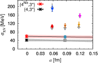
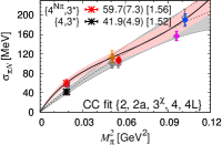
Figure 3: Data for the $\sigma$-term, $\sigma_{\pi N}={m}_{ud}g_{S}^{u+d}$, from the two ESC strategies $\{4,3^{\ast}\}$ (gray) and $\{4^{N\pi},3^{\ast}\}$ (color) are shown as a function of $a$ and $M_{\pi}^{2}$. The two left panels show the chiral-continuum (CC) fit $\{2,2a,3,4\}$ and the two right the CC fit $\{2,2a,3^{\chi},4,4L\}$ described in the text. The result at $M_{\pi}=135\mathop{\rm MeV}\nolimits$ and [$\chi^{2}$/dof] of the two fits are given in the legend.

It is important to point out that the values of $M_{1}$ and $M_{2}$ used in both fit strategies are an effective bundling of the many excited states that contribute into two. In fact, as mentioned above, many combinations of $M_{1}$ and $M_{2}$ between $\{4,3^{\ast}\}$ and $\{4^{N\pi},3^{\ast}\}$ (see Table 1) give fits with equally good $\chi^{2}$ values. Ref. [80] showed that for $\tau\gtrsim 1.0$ fm and for both fit strategies, the dominant ESC in $C^{3\text{pt}}$ comes from the first excited state. Thus, operationally, our two results for $\sigma_{\pi N}$ should be regarded as: what happens if the first “effective” excited state has $M_{1}\approx 1220\mathop{\rm MeV}\nolimits$ (motivated by $\chi$PT and corresponding to the lowest theoretically possible states $N\pi$ or $N\pi\pi$) versus $1600\mathop{\rm MeV}\nolimits$ obtained from the standard fit to the 2-point function. To further resolve all the excited states that contribute significantly and their energies in a finite box requires much higher precision data on additional $M_{\pi}\approx 135$ MeV ensembles. In short, while our $\{4^{N\pi},3^{\ast}\}$ analysis reconciles the lattice and the phenomenological values, it also calls for validation in future calculations.

III Excited states in $\boldsymbol{\chi}$PT

The contributions of low-momentum $N\pi$ and $N\pi\pi$ states to $C^{\rm 2pt}$ and $C^{\rm 3pt}$ can be studied in $\chi$PT [81, 82, 83, 84, 85, 86, 87, 88], a low-energy effective field theory (EFT) of QCD that provides a systematic expansion of $\mathcal{R}_{S}(\tau,t)$ in powers of $Q/\Lambda_{\chi}$, where $Q$ denotes a low-energy scale of order of the pion mass, $Q\in\{M_{\pi},t^{-1},(\tau-t)^{-1}\}$, while $\Lambda_{\chi}\approx 1\mathop{\rm GeV}\nolimits$ is the typical scale of QCD. In contrast to the isovector scalar charge considered in Ref. [83], we find large contributions from the $N(\bf{k})\pi(-\bf k)$ and $N(\bf{0})\pi({\bf{k}})\pi({-\bf{k}})$ states, which can give up to $30\%$ corrections to $\mathcal{R}_{S}$ and thus affect the extraction of $g_{S}^{u+d}$ and $\sigma_{\pi N}$ in a significant way.

The diagrams contributing to $\mathcal{R}_{S}$ are shown in Fig. 5, where we assume $\mathcal{N}(x)$ to be a local nucleon source with well defined transformation properties under chiral symmetry. The chiral representation of this class of sources has been derived in Refs. [89, 81, 82]. Details of the calculation at next-to-next-to-leading order (N²LO) in $\chi$PT and the expansion of $\mathcal{N}$ in terms of heavy nucleon and pion fields are summarized in App. B. The crucial observation is that the isoscalar scalar source couples strongly to two pions, so that loop diagrams with the scalar source emitting two pions, which are consequently absorbed by the nucleon, are suppressed by only one chiral order, $Q/\Lambda_{\chi}$. These diagrams have both $N\pi$ and $N\pi\pi$ cuts, which give rise to ESC to Euclidean Green’s functions. A second important effect is that the next-to-leading-order (NLO) couplings of the nucleon to two pions, parameterized in $\chi$PT by the low-energy constants (LECs) $c_{1,2,3}$, are sizable, reflecting the enhancement by degrees of freedom related to the $\Delta(1232)$. When the pions couple to the isoscalar source, these couplings give rise to large N²LO corrections that are dominated by $N\pi\pi$ excited states and have the same sign as the NLO correction. Since, in the isospin-symmetric limit, the isovector scalar source does not couple to two pions, the NLO diagrams and the N²LO diagrams proportional to $c_{1,2,3}$ do not contribute to the isovector 3-point function, whose leading ESC arises at $\mathcal{O}(Q^{2}/\Lambda^{2}_{\chi})$. A detailed analysis showing that the functional form of the ESC predicted by $\chi$PT matches the lattice data and fits for sufficiently large time separations $\tau$ is given in App. B. In particular, the NLO and N²LO ESC can each reduce $\sigma_{\pi N}$ at a level of $10\mathop{\rm MeV}\nolimits$, thus explaining the $\{4^{N\pi},3^{\ast}\}$ fits, i.e., a larger value when ESC is taken into account.

IV Analysis of lattice data

Examples of fits with strategies $\{4,3^{\ast}\}$ and $\{4^{N\pi},3^{\ast}\}$ to remove ESC and obtain $g_{S}^{u+d,\text{bare}}$ are shown in Fig. 2 and the results summarized in Table 1. The final results are obtained from fits to the sum of the connected and disconnected contributions. These values overlap in all cases with the sum of estimates from separate fits to $g_{S}^{u+d,\,\text{conn}}$ and $g_{S}^{2l}$. From the separate fits, we infer that most of the difference between the two ESC strategies comes from the disconnected diagrams, which we interpret as due to the $N\pi/N\pi\pi$ contributions through quark-level diagrams such as shown in Fig. 1.

Figure 3 shows data for $\sigma_{\pi N}={m}_{ud}^{\text{bare}}\ g_{S}^{u+d,\text{bare}}$ as a function of $a$ and $M_{\pi}^{2}$. The chiral-continuum (CC) extrapolation is carried out using the N²LO $\chi$PT expression [41]:

$$\sigma_{\pi N}=(d_{2}+d_{2}^{a}a)M_{\pi}^{2}+d_{3}M_{\pi}^{3}+d_{4}M_{\pi}^{4}+d_{4L}M_{\pi}^{4}\log\frac{M_{\pi}^{2}}{M_{N}^{2}}\,.$$ (4)

The $d_{i}$ in $\chi$PT (henceforth labeled $d_{i}^{\chi}$) are given in Eq. (15) and evaluated with $M_{N}=0.939\mathop{\rm GeV}\nolimits$, $g_{A}=1.276$, $F_{\pi}=92.3\mathop{\rm MeV}\nolimits$. Neglected finite-volume corrections can also be estimated in $\chi$PT, see App. B and Refs. [78, 90], indicating a correction of less than $1\mathop{\rm MeV}\nolimits$ for the $a09m130$ ensemble.

Figure 3 shows two chiral fits based on the N²LO $\chi$PT expression for $\sigma_{\pi N}$. The $\{2,2a,3,4\}$ fit keeps terms proportional to $\{d_{2},d_{2}^{a},d_{3},d_{4}\}$ with all coefficients free. In the $\{2,2a,3^{\chi},4,4L\}$ fit we use the $\chi$PT value for $d_{3}=d_{3}^{\chi}$, which does not involve any LECs, and include the $d_{4L}$ term. Each panel also shows the six data points obtained with the $\{4,3^{\ast}\}$ and $\{4^{N\pi},3^{\ast}\}$ strategies and the fits to them. In each fit $d_{2}^{a}$ comes out consistent with zero.

The results for $\sigma_{\pi N}$ at the physical point $M_{\pi}=135\mathop{\rm MeV}\nolimits$ from the various fits are essentially given by the $a09m130$ point. We have neglected a correction due to flavor mixing inherent in Wilson-clover fermions since it is small as shown in App. D. Our final result, $\sigma_{\pi N}=59.6(7.4)$ MeV, is the average of results from the $\{2,2a,3,4\}$ and $\{2,2a,3^{\chi},4,4L\}$ fits to the $\{4^{N\pi},3^{\ast}\}$ data given in Fig. 3, which overlap. In App. B, we consider more constrained fit variants, which show that the fit coefficients of the $M_{\pi}^{2}$ and $M_{\pi}^{4}\log M_{\pi}^{2}$ terms are also broadly consistent with their $\chi$PT prediction.

V Conclusions

Results for $\sigma_{\pi N}$ were reviewed by FLAG in 2019 [72], and there have been two new calculations since as summarized in App. E, and shown in Fig. 4. The ETM collaboration [69], using the direct method on one physical mass 2+1+1-flavor twisted mass clover-improved ensemble, obtained $\sigma_{\pi N}=41.6(3.8)\mathop{\rm MeV}\nolimits$; the BMW collaboration using the FH method and 33 ensembles of 1+1+1+1-flavor Wilson-clover fermions [70], but all with $M_{\pi}>199\mathop{\rm MeV}\nolimits$, find $\sigma_{\pi N}=37.4(5.1)\mathop{\rm MeV}\nolimits$. The $\chi$PT analysis of the impact of low-lying excited $N\pi$ states in the FH and direct methods is the same, and as shown in Fig. 3, it mainly affects the behavior for $M_{\pi}\lesssim 135\mathop{\rm MeV}\nolimits$. Our work indicates that previous lattice calculations give the lower value $\sigma_{\pi N}\approx 40\mathop{\rm MeV}\nolimits$ because in the FH analysis [70] the fit ansatz (Taylor or Padé) parameters are determined using $M_{\pi}\geq 199\mathop{\rm MeV}\nolimits$ data, and in the direct method, the $N\pi/N\pi\pi$ states have not been included when extracting the ground-state matrix element [69].

Ensemble ID	$a$ (fm)	$M_{\pi}$ (MeV)	$(L/a)^{3}\times T/a$	$M_{\pi}L$	$N_{\text{conf}}^{\rm 2pt}$	$N_{\text{conf}}^{\rm conn}$	$N_{\text{LP}}$	$N_{\text{HP}}$	$N_{\text{conf}}^{l}$	$N_{\text{src}}^{l}$	$N_{\rm LP}^{l}/N_{\rm HP}^{l}$
$a12m310$	0.1207(11)	310(3)	$24^{3}\times 64$	4.55	1013	1013	64	8	1013	5000	30
$a12m220$	0.1184(10)	228(2)	$32^{3}\times 64$	4.38	959	744	64	4	958	11000	30
$a09m310$	0.0888(08)	313(3)	$32^{3}\times 96$	4.51	2263	2263	64	4	–	–	–
$a09m220$	0.0872(07)	226(2)	$48^{3}\times 96$	4.79	964	964	128	8	712	8000	30
$a09m130$	0.0871(06)	138(1)	$64^{3}\times 96$	3.90	1274	1290	128	4	1270	10000	50
$a06m310$	0.0582(04)	320(2)	$48^{3}\times 144$	4.52	977	500	128	4	808	12000	50
$a06m220$	0.0578(04)	235(2)	$64^{3}\times 144$	4.41	1010	649	64	4	1001	10000	50

Table 2: Lattice parameters of the six ensembles analyzed for the isoscalar scalar charge $g_{S}^{u+d}$. Columns 6–9 give the number of configurations analyzed, and the number of low- (high-) precision measurements made per configuration for the connected contributions. Columns 10–12 give the number of configurations, low-precision random sources used, and the ratio $N_{\rm LP}/N_{\rm HP}$ for the disconnected contributions. The analysis of the isovector contributions has been presented in Ref. [78]. The ensemble $a09m310$ has been used only in the analysis of the nucleon mass in App. C.

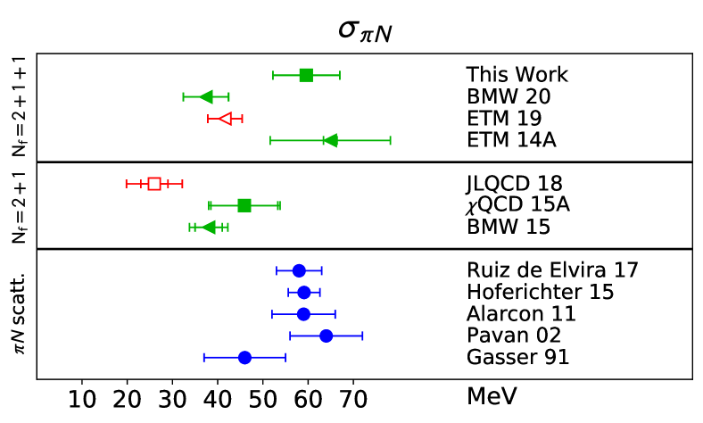
Figure 4: Results for $\sigma_{\pi N}={m}_{ud}g_{S}^{u+d}$ from 2+1- and 2+1+1-flavor lattice calculations. The BMW 20 result from 1+1+1+1-flavor lattices is listed along with the other 2+1+1-flavor calculations for brevity. Following the FLAG conventions, determinations via the direct approach are indicated by squares and the FH method by triangles. Also, the symbols used for lattice estimates that satisfy the FLAG criteria for inclusion in averages are filled green, and those not included are open red. The references from which lattice results have been taken are: JLQCD 18 [68], $\chi$QCD 15A [65], BMW 15 [64], ETM 14A [71], ETM 19 [69], and BMW 20 [70]. Phenomenological estimates using $\pi N$ scattering data (blue filled circles) are from Gasser 91 [20], Pavan 02 [26], Alarcon 11 [28], Hoferichter 15 [39], and Ruiz de Elvira 17 [45].

To conclude, a $\chi$PT analysis shows that the low-lying $N\pi$ and $N\pi\pi$ states can make a significant contribution to $g_{S}^{u+d}$. Including these states in our analysis (the $\{4^{N\pi},3^{\ast}\}$ strategy) gives $\sigma_{\pi N}=59.6(7.4)\mathop{\rm MeV}\nolimits$, whereas the standard analysis ($\{4,3^{\ast}\}$ strategy) gives $\sigma_{\pi N}=41.9(4.9)\mathop{\rm MeV}\nolimits$ consistent with previous analyses [72]. These chiral fits are shown in Fig. 3. Since the $\{4,3^{\ast}\}$ and $\{4^{N\pi},3^{\ast}\}$ strategies to remove ESC are not distinguished by the $\chi^{2}$ of the fits, we provide a detailed N²LO $\chi$PT analysis of ESC, which reveals sizable corrections consistent with the $\{4^{N\pi},3^{\ast}\}$ analysis, restoring agreement with phenomenology. Since the effect of the $N\pi$ and $N\pi\pi$ states becomes significant near $M_{\pi}=135\mathop{\rm MeV}\nolimits$, further work on physical mass ensembles is needed to validate our result and to increase the precision in the extraction of the nucleon isoscalar scalar charge.

Appendix A Details of the Lattice Analysis

The parameters of the seven 2+1+1-flavor ensembles generated using the HISQ action [75] by the MILC collaboration [76] are given in Table 2. Note that the seventh ensemble, $a09m310$, listed has been used only for the analysis of the nucleon mass in App. C. On each of these ensembles, the calculations of the 2- and 3-point functions was carried out using tadpole improved Wilson-clover fermions as described in Ref. [78].

To reduce ESC, smeared sources using the Wuppertal method [92] were used to generate quark propagators with parameters given in Ref. [78]. The same smearing was used at the source and sink points.

All correlation functions are constructed using the truncated solver method with bias correction [93, 94, 78]. In this method, high statistics are obtained by using a low-precision (LP) stopping criterion in the inversion of the quark propagators, which was taken to be between $r_{\rm LP}\equiv|{\rm residue}|_{\rm LP}/|{\rm source}|=10^{-3}$ and $5\times 10^{-4}$. These estimates are corrected for possible bias using high-precision (HP) measurements with $r_{\rm HP}$ taken to be between $10^{-7}$ and $10^{-8}$ [77, 78]. The number of configurations analyzed, and the number of LP and HP measurements made for the connected and disconnected contributions, are given in Table 2. In our data, the bias correction term was found to be a fraction of the $1\sigma$ error in all quantities and for all six ensembles.

For the statistical analysis of the data, we first constructed bias-corrected values for the 2- and 3-point correlation functions, then averaged these over the multiple measurements made on each configuration, and finally binned these. These binned data, 250–320 depending on the ensemble, were analyzed using the single elimination jackknife process. The analysis was repeated to quantify model variation of results by choosing data with different set of source-sink separations $\tau$ and different number of points $t_{\text{skip}}$, next to the source and the sink for each $\tau$, skipped in the excited-state fits. The final result was taken to be the average over the model values, weighting each by its Akaike information criteria weight.

The bare quark mass is defined to be $m_{ud}^{\text{bare}}=1/2\kappa_{l}-1/2\kappa_{c}$, with the critical value of the hopping parameter, $\kappa_{c}$, determined using a linear fit to $(aM_{\pi})^{2}$ versus $1/2\kappa$ at each of the three values of $a$. Results for $M_{\pi}$ are given in Table 2 and fits to the nucleon mass are discussed in App. C. A subtle point in the renormalization of $\sigma_{\pi N}$ for Wilson-clover fermions is presented in App. D.

The final quoted errors are from the chiral fits shown in Fig. 3 and given in the labels. The error in each data point, $\sigma_{\pi N}=m^{\rm bare}_{ud}\times g_{S}^{u+d,{\rm bare}}$, combines in quadrature those in $m^{\rm bare}_{ud}$ and $g_{S}^{u+d,{\rm bare}}$ (see Table 1), with the latter given by the appropriate fit used to remove the ESC as illustrated in Fig. 2.

In addition to the simultaneous fits to $C^{2\text{pt}}$ and $C^{3\text{pt}}$ to remove ESC, we have also carried out the full analysis by first calculating the $M_{i}$ from 4-state fits to $C^{2\text{pt}}$ and using these as input in 3-state fits to $C^{3\text{pt}}$ as described in Ref. [80]. The priors used for the excited state masses $M_{i}$ and the amplitudes $\mathcal{A}_{i}$ are given in Table 5 in App. C. The two sets of results for $M_{i}$ from the two approaches (simultaneous versus individual fits) are consistent and the ground state matrix elements agree within $1\sigma$. This agreement occurs for both strategies, $\{4,3^{\ast}\}$ and $\{4^{N\pi},3^{\ast}\}$. The error estimates from the simultaneous fits used to get the final results are slightly larger.

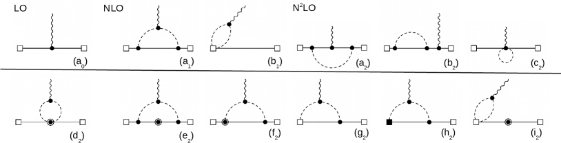
Figure 5: Corrections to the scalar charge in $\chi$PT. An empty and full square denote, respectively, an insertion of the LO and NLO expansion of the source fields $\mathcal{N}$ and $\bar{\mathcal{N}}$. Plain, dashed, and wavy lines denote, respectively, nucleons, pions, and an insertion of the scalar source. Dots and circled dots denote LO and NLO vertices in the chiral Lagrangian. We show one diagram for each topology, and the inclusion of all the possible orderings is understood. Diagrams $(g_{2})$, $(h_{2})$, and $(i_{2})$ are representative of N²LO corrections arising from the chiral expansion of $\mathcal{N}$. We do not consider these diagrams in our calculation, as they only produce N²LO recoil corrections (including $(g_{2})$ despite containing only LO interactions [81, 82]).

Appendix B Chiral Perturbation Theory

The corrections to the nucleon mass and the $\sigma$-term in $\chi$PT have a long history in the literature [95, 74, 96, 17, 97, 98, 99, 100, 101, 102, 18, 103, 104, 105]. The LO, NLO, and N²LO diagrams contributing to the isoscalar scalar charge $g_{S}^{u+d}$ are shown in Fig. 5. In these diagrams, plain and dashed lines denote pions and nucleons in the interaction picture of $\chi$PT, and not the nucleon and pion eigenstates of the full theory.

		NLO		N2LO		$\delta\sigma_{\pi N}(16,8)$	NLO		N2LO		$\delta\sigma_{\pi N}(12,6)$
$|\mathbf{n}_{\text{max}}|$	$m_{\mathbf{n}}$	loop	source	$c_{i}$	recoil	total	loop	source	$c_{i}$	recoil	total
$0$	$1$	$0$	$-0.4$	$-1.0$	$-0.0$	$-1.4$	$0$	$-0.5$	$-1.2$	$-0.1$	$-1.7$
$1$	$6$	$-2.2$	$-0.6$	$-2.9$	$-0.2$	$-5.9$	$-2.7$	$-0.9$	$-4.3$	$-0.2$	$-8.0$
$\sqrt{2}$	$12$	$-4.4$	$-0.8$	$-4.6$	$-0.3$	$-10.0$	$-5.6$	$-1.2$	$-7.4$	$-0.3$	$-14.5$
$\sqrt{3}$	$8$	$-5.2$	$-0.8$	$-5.2$	$-0.3$	$-11.6$	$-6.7$	$-1.3$	$-8.7$	$-0.4$	$-17.1$
$2$	$6$	$-5.6$	$-0.9$	$-5.5$	$-0.3$	$-12.2$	$-7.3$	$-1.3$	$-9.4$	$-0.4$	$-18.4$
$\sqrt{5}$	$24$	$-6.5$	$-0.9$	$-6.2$	$-0.3$	$-14.0$	$-8.9$	$-1.4$	$-11.1$	$-0.5$	$-21.9$
$\sqrt{6}$	$24$	$-7.2$	$-0.9$	$-6.7$	$-0.4$	$-15.2$	$-10.1$	$-1.5$	$-12.4$	$-0.5$	$-24.5$
$\sqrt{8}$	$12$	$-7.4$	$-0.9$	$-6.8$	$-0.4$	$-15.5$	$-10.4$	$-1.5$	$-12.8$	$-0.5$	$-25.2$
$3$	$30$	$-7.7$	$-0.9$	$-7.0$	$-0.4$	$-16.0$	$-11.1$	$-1.6$	$-13.5$	$-0.5$	$-26.6$
$\infty$		$-9.2$	$-0.9$	$-7.6$	$-0.4$	$-18.0$	$-14.2$	$-1.5$	$-16.3$	$-0.6$	$-32.6$

Table 3: Excited-state corrections to the $\sigma$-term (in MeV). $\delta\sigma_{\pi N}(\tau,t)$, defined in Eq. (16), is evaluated for $t=\tau/2=8a$ (left) and $t=\tau/2=6a$ (right), using the parameters of the $a09m130$ lattice ensemble listed in Table 2. $|\mathbf{n}_{\text{max}}|$ denotes the maximum momentum included in the sum in Eqs. (B), (B), and (B), $m_{\mathbf{n}}$ the multiplicity of the momentum state [106]. We split the NLO corrections in Eq. (B) into the loop diagram $(a_{1})$ in Fig. 5, which also contributes to the ground state, and the diagram in which the scalar source couples to pions emitted by the nucleon source $\mathcal{N}$. At N²LO, we label by $c_{i}$ the contributions in Eq. (B) and by “recoil” those in Eq. (B). The last line is evaluated in the continuum.

These diagrams lead to the expansion

$$g_{S}^{u+d}=g_{S}^{(0)}+g_{S}^{(1)}\frac{M_{\pi}}{\Lambda_{\chi}}+g_{S}^{(2)}\frac{M_{\pi}^{2}}{\Lambda_{\chi}^{2}}+\ldots,$$ (5)

where $\Lambda_{\chi}=4\pi F_{\pi}\approx 1$ GeV is the breakdown scale of the chiral expansion. The NLO diagrams $(a_{1})$ and $(b_{1})$ in Fig. 5 only contribute to the isoscalar channel, implying that the isovector channel has the different expansion

$$g_{S}^{u-d}=\tilde{g}_{S}^{(0)}+\tilde{g}_{S}^{(2)}\frac{M_{\pi}^{2}}{\Lambda_{\chi}^{2}}+\ldots$$ (6)

We will show that the same loop diagrams responsible for the NLO and N²LO corrections to $g_{S}$ also induce a sizable contribution from $N\pi$ and $N\pi\pi$ intermediate states.

To this end, we calculate the ratio $\mathcal{R}_{S}(\tau,t)$ using heavy-baryon $\chi$PT and expand it as

$$\mathcal{R}(\tau,t)=\mathcal{R}^{(0)}(\tau,t)+\mathcal{R}^{(1)}(\tau,t)+\mathcal{R}^{(2)}(\tau,t),$$ (7)

including in its definition a factor $m_{ud}$ to make the result $\mathcal{R}=m_{ud}\mathcal{R}_{S}$ scale independent and ensure a normalization that facilitates the comparison to $\sigma_{\pi N}$. We assume $\mathcal{N}$ to be a local nucleon source, transforming as $\left(\frac{1}{2},0\right)\oplus\left(0,\frac{1}{2}\right)$ under the chiral group $SU(2)_{L}\otimes SU(2)_{R}$. The heavy-baryon $\chi$PT realization of $\mathcal{N}$ was constructed in Ref. [82]

$$\mathcal{N}(x)=\left[\left(1-\frac{\boldsymbol{\pi}^{2}}{8F_{\pi}^{2}}\right)-i\frac{\boldsymbol{\pi}\cdot\boldsymbol{\tau}}{2F_{\pi}}\gamma_{5}\right]N_{v}+\mathcal{O}\left(\frac{1}{M_{N}}\right),$$ (8)

where $N_{v}=(1+\gamma_{4})N_{v}/2$ represents a heavy-nucleon field. At $\mathcal{O}(1/M_{N})$, Eq. (8) contains additional LECs, which reduce the predictive power of the calculation.

At LO one simply has $\mathcal{R}^{(0)}=m_{ud}g_{S}^{(0)}$. The NLO diagrams receive contributions from nucleon, $N\pi$, and $N\pi\pi$ excited states, leading to

$$\mathcal{R}^{(1)}(\tau,t) =\frac{3g^{2}_{A}M_{\pi}^{2}}{8F_{\pi}^{2}L^{3}}\sum_{\mathbf{k}}\frac{\mathbf{k}^{2}}{E_{\pi}^{4}}\bigg{[}1-e^{-E_{N\pi}t}-e^{-E_{N\pi}t_{B}}$$

$$+\frac{1}{2}e^{-E_{N\pi}\tau}+\frac{1}{4}e^{-2E_{\pi}t}+\frac{1}{4}e^{-2E_{\pi}t_{B}}\bigg{]}$$

$$-\frac{3M_{\pi}^{2}}{32F_{\pi}^{2}}\frac{1}{L^{3}}\sum_{\mathbf{k}}\frac{1}{E_{\pi}^{2}}\left(e^{-2E_{\pi}t}+e^{-2E_{\pi}t_{B}}\right),$$ (9)

where $E_{\pi}=\sqrt{\mathbf{k}^{2}+M_{\pi}^{2}}$, $\widetilde{E}_{N}=\sqrt{M_{N}^{2}+\mathbf{k}^{2}}-M_{N}$, $E_{N\pi}=E_{\pi}+\tilde{E}_{N}$, $\mathbf{k}=2\pi\mathbf{n}/L$, and $t_{B}=\tau-t$. $F_{\pi}=92.3\mathop{\rm MeV}\nolimits$ is the pion decay constant, $g_{A}=1.276$ the axial charge of the nucleon [107]. The first term in Eq. (B) is a correction to the ground-state contribution

$$\frac{3g^{2}_{A}M_{\pi}^{2}}{8F_{\pi}^{2}}\frac{1}{L^{3}}\sum_{\mathbf{k}}\frac{\mathbf{k}^{2}}{E_{\pi}^{4}}=-\frac{9g^{2}_{A}M_{\pi}^{3}}{64\pi F_{\pi}^{2}}+\Delta_{L}\sigma_{\pi N},$$ (10)

where $\Delta_{L}\sigma_{\pi N}$ is the finite-volume correction to the $\sigma$-term [108]. The remaining terms reflect the excited states, with diagram $(a_{1})$ receiving a contribution from $N\pi$ intermediate states (nucleon and pion having opposite momenta) and from an $N\pi\pi$ state (the nucleon at rest and the two pions carrying momenta $\pm\mathbf{k}$). The $N\pi$ and $N\pi\pi$ states with zero pion momentum vanish due to the prefactor $\mathbf{k}^{2}$. The amplitude of the $N\pi$ contribution is suppressed by $(M_{\pi}L)^{3}$ compared to $g_{S}^{(0)}$, but enhanced by the large coupling of a scalar source to the pion, making it suppressed by only a single chiral order. The last line of Eq. (B) originates from diagram $(b_{1})$. In this case the dominant excited state is $N\pi\pi$, with the two pions at zero momentum. Diagram $(g_{2})$ arises from the last term in the square bracket in Eq. (8). Though formally NLO, this diagram vanishes up to $\mathcal{O}(1/M_{N})$ corrections, and thus the topology $(g_{2})$ only contributes to N²LO. Similarly, the diagram with the pion emitted by $\mathcal{N}$ and absorbed by $\bar{\mathcal{N}}$ vanishes at NLO.

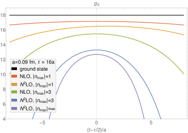
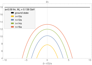
Figure 6: (Left) Excited-state corrections from different truncations to the isoscalar scalar charge $g_{S}$ in $\chi$PT. (Right) Estimates for ${\cal R}_{S}(\tau,t)$ from the N²LO analysis for the $a09m130$ ensemble, which should be compared to the data in Fig. 2 (and the shape with that of the separate contributions shown in Fig. 7). We assume $g_{S}=18$ is the asymptotic value in both cases.

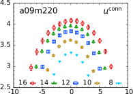
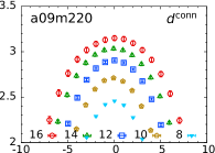
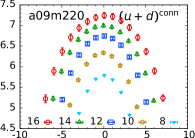
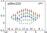
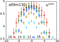
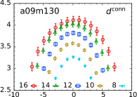
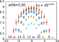
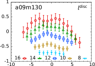
Figure 7: Data for the ratio ${\cal R}_{\mathcal{S}}=C({\rm 3pt})/C({\rm 2pt})$ for $\tau/a$ listed in the label are shown for the $u$, $d$, and $(u+d)$ connected, and light quark $l$ disconnected contributions, and plotted versus $(t-\tau/2)/a$ for the $a09m220$ (top) and $a09m130$ (bottom) ensembles.

At N²LO there are several contributions. They come from loop corrections to the LO (diagrams $(a_{2})$, $(b_{2})$, and $(c_{2})$) and from diagrams with subleading interactions in the chiral Lagrangian and the scalar source coupling to two pions (diagrams $(d_{2})$, $(e_{2})$, and $(f_{2})$). Here, diagrams $(a_{2})$ and $(b_{2})$ are exactly canceled by the N²LO corrections to the 2-point function. This is in contrast to the isovector case, in which they are responsible for the leading ESC:

$$\mathcal{R}^{(2)}_{\text{isovector}}(\tau,t) =-m_{ud}\tilde{g}^{(0)}_{S}\frac{g_{A}^{2}}{2F_{\pi}^{2}}\frac{1}{L^{3}}\sum_{\mathbf{k}}\frac{\mathbf{k}^{2}}{E^{3}_{\pi}}$$

$$\times\bigg{[}1-e^{-E_{\pi}t}-e^{-E_{\pi}t_{B}}+e^{-E_{\pi}\tau}\bigg{]}.$$ (11)

This result agrees with the corrections to the isovector scalar charge computed in Ref. [83], once we expand in the limit $M_{N}\gg|\mathbf{k}|$.

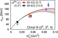
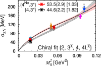
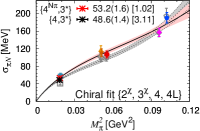
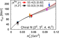
Figure 8: Chiral fits to the data for the $\sigma$-term, $\sigma_{\pi N}={m}_{ud}g_{S}^{u+d}$, from the two ESC strategies $\{4,3^{\ast}\}$ (gray) and $\{4^{N\pi},3^{\ast}\}$ (color) shown as a function of $M_{\pi}^{2}$. The four chiral fits are $\{2^{\chi},3^{\chi},4\}$, $\{2,3^{\chi},4,4L^{\chi}\}$, $\{2^{\chi},3^{\chi},4,4L\}$, and $\{2^{\chi},3^{\chi},4,4L^{\chi}\}$. The result at $M_{\pi}=135\mathop{\rm MeV}\nolimits$ and the [$\chi^{2}$/dof] of the chiral fit for the two ESC strategies are given in the legend.

chiral fit	$\{4,3^{\ast}\}$						$\{4^{N\pi},3^{\ast}\}$
	$d_{2}$	$d_{3}$	$d_{4}$	$d_{4L}$	$\frac{\chi^{2}}{\text{dof}}$	$\sigma_{\pi N}$	$d_{2}$	$d_{3}$	$d_{4}$	$d_{4L}$	$\frac{\chi^{2}}{\text{dof}}$	$\sigma_{\pi N}$
	$(\text{GeV}^{-1})$	$(\text{GeV}^{-2})$	$(\text{GeV}^{-3})$	$(\text{GeV}^{-3})$		(MeV)	$(\text{GeV}^{-1})$	$(\text{GeV}^{-2})$	$(\text{GeV}^{-3})$	$(\text{GeV}^{-3})$		(MeV)
$\chi$PT	$4.44$	$-8.55$	–	$11.35$	–	–	$4.44$	$-8.55$	–	$11.35$	–	–
$\{2,3\}$	$2.56(26)$	$-2.77(98)$	–	–	$0.83$	$39.8(2.4)$	$3.30(36)$	$-5.1(1.3)$	–	–	$1.63$	$47.7(3.5)$
$\{2,3,4\}$	$2.49(94)$	$-2.1(8.1)$	$-1(17)$	–	$1.11$	$39.7(3.3)$	$6.0(1.7)$	$-27(13)$	$42(26)$	–	$1.28$	$57.4(6.9)$
$\{2^{\chi},3^{\chi},4\}$	$4.44$	$-8.55$	$-3.11(75)$	–	$13.4$	$58.82(25)$	$4.44$	$-8.55$	$-1.25(70)$	–	$3.71$	$59.44(23)$
$\{2,3^{\chi},4,4L\}$	$2.84(53)$	$-8.55$	$0.2(15.6)$	$-7.0(9.3)$	$1.13$	$39.8(3.3)$	$5.1(1.0)$	$-8.55$	$41(23)$	$22(15)$	$1.21$	$57.7(6.8)$
$\{2,3^{\chi},4,4L^{\chi}\}$	$3.84(15)$	$-8.55$	$30.8(2.0)$	$11.35$	$1.82$	$44.6(2.2)$	$4.45(20)$	$-8.55$	$24.6(2.4)$	$11.35$	$1.03$	$53.5(2.9)$
$\{2^{\chi},3^{\chi},4,4L\}$	$4.44$	$-8.55$	$43.3(6.3)$	$19.9(2.7)$	$3.11$	$48.6(1.4)$	$4.44$	$-8.55$	$25.4(7.0)$	$11.7(3.1)$	$1.02$	$53.2(1.6)$
$\{2^{\chi},3^{\chi},4,4L^{\chi}\}$	$4.44$	$-8.55$	$23.40(75)$	$11.35$	$4.50$	$53.01(25)$	$4.44$	$-8.55$	$24.64(70)$	$11.35$	$0.82$	$53.42(23)$

	$d_{2}$	$d_{2}^{a}$	$d_{3}$	$d_{4}$	$d_{4L}$	$\frac{\chi^{2}}{\text{dof}}$	$\sigma_{\pi N}$	$d_{2}$	$d_{2}^{a}$	$d_{3}$	$d_{4}$	$d_{4L}$	$\frac{\chi^{2}}{\text{dof}}$	$\sigma_{\pi N}$
	$(\text{GeV}^{-1})$		$(\text{GeV}^{-2})$	$(\text{GeV}^{-3})$	$(\text{GeV}^{-3})$		(MeV)	$(\text{GeV}^{-1})$		$(\text{GeV}^{-2})$	$(\text{GeV}^{-3})$	$(\text{GeV}^{-3})$		(MeV)
$\{2,2a,3,4\}$	$2.61(96)$	$-0.3(5)$	$-2.2(8.1)$	$-1(17)$	–	$1.49$	$41.8(4.9)$	$6.1(1.7)$	$-0.3(4)$	$-27(13)$	$42(26)$	–	$1.65$	$59.5(7.4)$
$\{2,2a,3^{\chi},4,4L\}$	$2.95(57)$	$-0.3(5)$	$-8.55$	$0.6(15.6)$	$-7.0(9.3)$	$1.52$	$41.9(4.9)$	$5.2(1.0)$	$-0.3(4)$	$-8.55$	$40(23)$	$21(15)$	$1.56$	$59.7(7.3)$

Table 4: Chiral fit coefficients with the ansatz $d_{2}M_{\pi}^{2}+d_{3}M_{\pi}^{3}+d_{4}M_{\pi}^{4}+d_{4L}M_{\pi}^{4}\log(M_{\pi}/M_{N})^{2}$. Here the $\chi$PT values for $d_{i}$ are calculated using Eq. (B) and with $M_{N}=0.939\mathop{\rm GeV}\nolimits$, $g_{A}=1.276$, $F_{\pi}=92.3\mathop{\rm MeV}\nolimits$. $d_{4L}$ includes the chiral logarithm in $\bar{l}_{3}=-\log M_{\pi}^{2}+$ finite. The lower table gives the coefficients for the fits including an $aM_{\pi}^{2}$ term, as discussed in Sec. IV.

Diagram $(c_{2})$ only contributes to the ground state, and diagrams $(d_{2})$ and $(e_{2})$ are recoil corrections. A first effect of these diagrams is to shift the energy excitation of the $N\pi$ state from $E_{\pi}$ to $E_{\pi}+\widetilde{E}_{N}$. The remaining recoil corrections are

$$\mathcal{R}^{(2)}_{\text{recoil}} =-\frac{9g^{2}_{A}M_{\pi}^{2}}{32M_{N}F_{\pi}^{2}L^{3}}\sum_{\mathbf{k}}\frac{(\mathbf{k}^{2})^{2}}{E_{\pi}^{5}}\bigg{[}1-\frac{2}{3}e^{-E_{\pi}t}$$

$$-\frac{2}{3}e^{-E_{\pi}t_{B}}+\frac{2}{3}e^{-E_{\pi}\tau}-\frac{1}{6}e^{-2E_{\pi}t}-\frac{1}{6}e^{-2E_{\pi}t_{B}}\bigg{]}$$

$$+\frac{3g_{A}^{2}M_{\pi}^{2}}{32M_{N}F_{\pi}^{2}L^{3}}\sum_{\mathbf{k}}\frac{1}{E_{\pi}}\bigg{[}1-\frac{1}{2}e^{-2E_{\pi}t}-\frac{1}{2}e^{-2E_{\pi}t_{B}}$$

$$+\frac{2\mathbf{k}^{2}}{E_{\pi}^{2}}\Big{(}1-e^{-E_{\pi}t}-e^{-E_{\pi}t_{B}}+e^{-E_{\pi}\tau}\Big{)}\bigg{]}.$$ (12)

Finally, diagram $(d_{2})$ receives contributions from the LECs $c_{1,2,3}$, which contribute to $\pi N$ scattering at NLO in $\chi$PT. Including diagram $(c_{2})$, they give

$$\mathcal{R}^{(2)}_{c_{i}} =-\frac{3M_{\pi}^{2}}{4F_{\pi}^{2}}\frac{1}{L^{3}}\sum_{\mathbf{k}}\frac{1}{E_{\pi}^{3}}\Big{(}(c_{2}+2c_{3})E_{\pi}^{2}$$

$$+(2c_{1}-c_{3})M_{\pi}^{2}\Big{)}\bigg{[}1-\frac{1}{2}e^{-2E_{\pi}t}-\frac{1}{2}e^{-2E_{\pi}t_{B}}\bigg{]}$$

$$+\frac{3M_{\pi}^{2}}{F_{\pi}^{2}}\frac{1}{L^{3}}\sum_{\mathbf{k}}\frac{1}{E_{\pi}}c_{1}.$$ (13)

The energy gap in this case is $\approx 2M_{\pi}$, since $\mathbf{k}=\boldsymbol{0}$ is allowed. The LECs $c_{1,2,3}$ have been determined most reliably by an analysis of $\pi N$ scattering using Roy–Steiner equations, matched to $\chi$PT in the subthreshold region [40, 41]. We will use the N³LO values

$$c_{1} =-1.11(3)\mathop{\rm GeV}\nolimits^{-1},\qquad c_{2}=3.13(3)\mathop{\rm GeV}\nolimits^{-1},$$

$$c_{3} =-5.61(6)\mathop{\rm GeV}\nolimits^{-1},$$ (14)

which correspond to N²LO in the scalar form factor. We neglect the N²LO diagrams with pions emitted by the nucleon source, represented by $(g_{2})$, $(h_{2})$, and $(i_{2})$ in Fig. 5, given that for a local source the NLO contribution is already small. Of these diagrams, $(g_{2})$ produces N²LO recoil corrections, $(h_{2})$ contains unknown LECs that appear in the expansion of the source, and $(i_{2})$ cancels in the ratio between the 2- and 3-point function. While we have assumed local nucleon sources, the relative importance of the diagrams in Fig. 5 depends on the details of the lattice realization of $\mathcal{N}$. However, for the Gaussian smearing applied in this work with $r_{s}\sim 0.6\,\text{fm}$, corrections in addition to diagram $(b_{1})$ scale as $(r_{s}M_{\pi})^{2}\sim 0.2$ and can therefore be neglected, see also Refs. [81, 109].

In the infinite-volume limit, the ground-state pieces of Eqs. (B), (B), and (B) reproduce the N²LO expression for the $\sigma$-term (in the form given in Ref. [41])

$$\sigma_{\pi N} =m_{ud}\frac{\partial{M_{N}}}{\partial m_{ud}}=m_{ud}g_{S}^{u+d}$$ (15)

$$=-4c_{1}M_{\pi}^{2}-\frac{9g_{A}^{2}M_{\pi}^{3}}{64\pi F_{\pi}^{2}}-\frac{3M_{\pi}^{4}}{64\pi^{2}F^{2}_{\pi}}\Big{(}2\log\frac{M_{\pi}^{2}}{M_{N}^{2}}+1\Big{)}$$

$$\times\Big{(}\frac{g_{A}^{2}}{M_{N}}-8c_{1}+c_{2}+4c_{3}\Big{)}$$

$$+2M_{\pi}^{4}\bigg{\{}e_{1}+\frac{3}{128\pi^{2}F^{2}_{\pi}}\Big{(}c_{2}-\frac{2g_{A}^{2}}{M_{N}}\Big{)}+\frac{c_{1}\big{(}\bar{l}_{3}-1\big{)}}{16\pi^{2}F_{\pi}^{2}}\bigg{\}},$$

except for the LO contribution proportional to $c_{1}M_{\pi}^{2}$, its quark-mass renormalization proportional to $\bar{l}_{3}-1$, and the N²LO LEC $e_{1}$, all of which only contribute to the ground state. All other terms in Eq. (15) can be obtained by replacing the finite-volume sum $1/L^{3}\sum_{\mathbf{k}}$ with infinite-volume integrals in Eqs. (B), (B), and (B).

To assess the importance of the $N\pi$ and $N\pi\pi$ contributions we define

$$\delta\sigma_{\pi N}(\tau,t)=\mathcal{R}(\tau,t)-\lim_{t,\tau\rightarrow\infty}\mathcal{R}(\tau,t).$$ (16)

The contributions to $\delta\sigma_{\pi N}$ from the NLO diagrams (including the formally N²LO correction from $\widetilde{E}_{N}$) and from the N²LO diagrams are evaluated in Table 3, using the parameters of the $a09m130$ lattice ensemble, for two choices of source–sink separation, $\tau=16a$ and $\tau=12a$. We list separately the corrections from diagram $(a_{1})$ and $(b_{1})$ in Fig. 5, as the first is dominated by $N\pi$ excited states, the second by $N\pi\pi$. Similarly, the N²LO corrections from the diagrams proportional to the LECs $c_{1,2,3}$ receive contributions from $N\pi\pi$ states, while the recoil corrections in Eq. (B) are dominated by $N\pi$. From Table 3 we see that $\mathcal{R}^{(1)}$ and $\mathcal{R}^{(2)}$ are of similar size and the most important contributions come from diagram $(a_{1})$ and from Eq. (B). The nucleon source and recoil contributions are substantially smaller.

We also note that the ESC is amplified by the presence of several states close in energy. We can see this in the left panel of Fig. 6, where the red and orange curves denote the NLO and N²LO corrections, including states up to $|\mathbf{n}_{\text{max}}|=1$, while the green and blue curves include states up to $|\mathbf{n}_{\text{max}}|=3$. In the continuum, the effect of the entire tower of excited states can be resummed, with the result shown in the last line of Table 3 and by the purple line in Fig.  6. The comparison to the different $|\mathbf{n}_{\text{max}}|$ values indicates the degree of convergence, which is ultimately determined by $t$ and $\tau$ via the exponential suppression of the continuum integrals. Indeed, we see that for $\tau=16a$ the corrections at $t=8a$ beyond $|\mathbf{n}_{\text{max}}|=3$ are around $10\%$, but twice as large for $\tau=12a$, $t=6a$.

Away from $t\sim\tau/2$, the integrals become increasingly dominated by large-momentum modes, leading to the eventual breakdown of the chiral expansion. For this reason, the expansion becomes less reliable for small and large $t$, which explains why the functional form predicted by $\chi$PT, see the right panel of Fig. 6, suggests a faster decrease towards the edges than observed in the lattice data, see Figs. 2 and 7. (Note that in fits to remove the excited-state effects in the lattice data, we neglect $t_{\rm skip}$ points next to the source and the sink for each $\tau$.) In the center, however, the EFT expansion should be reliable, in particular for the $\tau=16a$ variant, which leads to the conclusion that NLO and N²LO contributions can each lead to a reduction of $\sigma_{\pi N}$ at the level of $10\mathop{\rm MeV}\nolimits$. Note that Fig. 7 shows the behavior versus $t$ and $\tau$ for the individual contributions, i.e., insertions on the $u$, the $d$, and the disconnected loop $l$.

While in Table 3 and Fig. 6 we focused on the ensemble with the lightest pion mass, we find good agreement between the $\chi$PT expectations and the fits in Fig. 2 also for the remaining ensembles. For example, with the parameters of the $a09m220$ ensemble, $\chi$PT predicts the difference between the lattice data and the extrapolated value of $g_{S}$ to be $3$ at $t=\tau/2=8a$, in good agreement with the left panel in the second row of Fig. 2. Similarly, for the $a06m220$ and $a06m310$ ensembles we obtain that $g_{S}$ is shifted by $2.8$ and $1.6$, at $t=\tau/2=12a$.

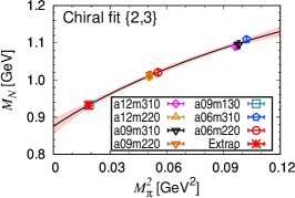
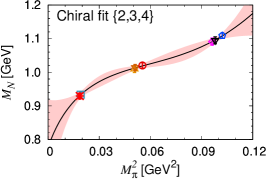
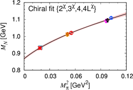
Figure 9: Chiral fits to the $\{4^{N\pi},3^{\ast}\}$ data for the nucleon mass $M_{0}$ given in Table 1. Data at a seventh point, $a09m310$, is included from Ref. [78]. The fit in the middle panel is overparameterized. The right panel shows that the $\{2^{\chi},3^{\chi},4,4L^{\chi}\}$ fit, with $\chi$PT values for three of the coefficients taken from Ref. [41], is reasonable and comparable to the fit in the left panel.

Finally, using Eq. (15), we have carried out the following chiral fits to the lattice data: $\{2,3\}$, $\{2^{\chi},3^{\chi},4\}$, $\{2,3^{\chi},4,4L^{\chi}\}$, $\{2^{\chi},3^{\chi},4,4L\}$, and $\{2^{\chi},3^{\chi},4,4L^{\chi}\}$, in addition to the fits $\{2,3,4\}$, $\{2,3^{\chi},4,4L\}$ already shown in Fig. 3. Four of these additional fits are shown in Fig. 8, with resulting fit parameters given in Table 4. (We neglect possible discretization errors in these fits as they are not resolved in our best fits shown in Fig. 3.) We see that for the $\{4^{N\pi},3^{\ast}\}$ strategy all fit variants lead to parameters that agree with the $\chi$PT prediction (including evidence for the nonanalytic $M_{\pi}^{3}$ term from the $\{2,3\}$ and $\{2,3,4\}$ fits), with changes in $\sigma_{\pi N}$ consistent with the uncertainty assigned to the least constrained fits ($\{2,3,4\}$ and $\{2,3^{\chi},4,4L\}$), whose average we quoted as our central result. Even in the most-constrained case $\{2^{\chi},3^{\chi},4,4L^{\chi}\}$ a good fit of the data is obtained, in marked contrast to the $\{4,3^{\ast}\}$ strategy, in which case the $\chi^{2}/\text{dof}$ becomes unacceptable when imposing the maximum amount of chiral constraints.

The expressions in Eqs. (B), (10), and (B) can also be used to assess the importance of finite-volume corrections to $g_{S}$. Focusing on the ground-state contributions, we can write $\Delta_{L}\sigma_{\pi N}$ in Eq. (10) as [108]

$$\Delta_{L}\sigma_{\pi N}=-\frac{3g_{A}^{2}M_{\pi}^{3}}{64\pi F_{\pi}^{2}}\sum_{\mathbf{n}\neq{\bf 0}}e^{-M_{\pi}L|\mathbf{n}|}\left(1-\frac{2}{M_{\pi}L|\mathbf{n}|}\right).$$ (17)

Similarly, for the $c_{i}$ contributions (B) we obtain

$$\Delta^{(2)}_{L}\sigma_{\pi N} =-\frac{3M_{\pi}^{4}}{8\pi^{2}F_{\pi}^{2}}\sum_{\mathbf{n}\neq{\bf 0}}\Big{[}(2c_{1}-c_{3})K_{0}(M_{\pi}L|\mathbf{n}|)$$

$$+(c_{2}+2c_{3}-4c_{1})\frac{K_{1}(M_{\pi}L|\mathbf{n}|)}{M_{\pi}L|\mathbf{n}|}\Big{]},$$ (18)

in terms of the Bessel functions $K_{0}$ and $K_{1}$. Using the parameters of the $a09m130$ lattice ensemble, we get

$$\Delta_{L}\sigma_{\pi N}=-0.77\mathop{\rm MeV}\nolimits,\quad\Delta^{(2)}_{L}\sigma_{\pi N}=-0.43\mathop{\rm MeV}\nolimits,$$ (19)

implying that the finite-volume corrections are controlled at the level of about $1\mathop{\rm MeV}\nolimits$.

We end this appendix by pointing out a subtlety. We have used the lowest-order (linear) relation between $M_{\pi}^{2}$ and $1/2\kappa$ to get $m_{ud}^{\text{bare}}$ as we have ensembles at only two values of $M_{\pi}$ at each $a$. Higher-order corrections give the LEC $\bar{l}_{3}$ term in Eq. (15). Removing it changes the $\chi$PT prediction of the $d_{4L}$ term in Table 4 from 11.35 to 9.70, however, the results of the $\{2,3^{\chi},4,4L^{\chi}\}$ and $\{2^{\chi},3^{\chi},4,4L^{\chi}\}$ fits do not change significantly.

Appendix C Chiral fits to the Nucleon Mass

Ensemble ID	Fit strategy	$r_{1}$	$a\Delta M_{1}$	$r_{2}$	$a\Delta M_{2}$	$r_{3}$	$a\Delta M_{3}$
$a12m310$	$\{4\}$	0.20(10)	0.40(15)	0.8(4)	0.6(2)	0.6(4)	0.4(2)
	$\{4^{N\pi}\}$	0.20(10)	0.37(05)	0.8(4)	0.6(2)	0.6(4)	0.4(2)
$a12m220$	$\{4\}$	0.40(20)	0.40(10)	1.0(6)	0.8(4)	0.8(6)	0.4(2)
	$\{4^{N\pi}\}$	0.40(30)	0.27(05)	1.0(8)	0.8(4)	0.8(6)	0.4(2)
$a09m310$	$\{4\}$	0.70(30)	0.30(05)	1.0(5)	0.5(2)	1.0(6)	0.5(3)
	$\{4^{N\pi}\}$	0.40(20)	0.28(05)	1.0(5)	0.5(3)	1.0(6)	0.5(3)
$a09m220$	$\{4\}$	0.60(30)	0.30(10)	0.8(5)	0.4(2)	0.7(4)	0.4(2)
	$\{4^{N\pi}\}$	0.35(20)	0.18(05)	0.8(5)	0.4(2)	0.7(4)	0.4(2)
$a09m130$	$\{4\}$	0.70(40)	0.30(10)	0.7(5)	0.5(3)	1.0(6)	0.3(2)
	$\{4^{N\pi}\}$	0.40(20)	0.12(02)	0.7(4)	0.3(1)	1.0(6)	0.3(2)
$a06m310$	$\{4\}$	0.50(30)	0.20(05)	1.0(6)	0.3(2)	1.0(6)	0.3(2)
	$\{4^{N\pi}\}$	0.50(30)	0.19(03)	1.0(6)	0.3(2)	1.0(6)	0.3(2)
$a06m220$	$\{4\}$	1.00(50)	0.25(10)	1.0(5)	0.3(1)	1.5(1.0)	0.3(2)
	$\{4^{N\pi}\}$	1.00(50)	0.14(03)	1.5(1.0)	0.2(1)	1.5(1.0)	0.3(2)

Table 5: The Bayesian priors and their width given within parenthesis used for the amplitude ratios $r_{i}\equiv|\mathcal{A}_{i}/\mathcal{A}_{0}|^{2}$ and mass differences $\Delta M_{i}\equiv M_{i}-M_{i-1}$ in the simultaneous fits to $C^{2\text{pt}}$ and $C^{3\text{pt}}$ for the two strategies $\{4,3^{\ast}\}$ and $\{4^{N\pi},3^{\ast}\}$.

In both types of analyses, simultaneous fits to $C^{2\text{pt}}$ and $C^{3\text{pt}}$ and individual fits to them, we have used the same empirical Bayesian priors for the amplitudes and masses of the three excited states determined using the procedure described in Ref. [78]. The central values of these priors and their widths for $\{4,3^{\ast}\}$ and $\{4^{N\pi},3^{\ast}\}$ fits are given in Table 5. The resulting $M_{0}$, $M_{1}$, and $M_{2}$ that enter in $\{3^{\ast}\}$ fits to $C^{3\text{pt}}$ are given in Table 1, and are essentially the same from the two types of analyses. The result for the nucleon mass on the seventh ensemble, $a09m310$, used only for the analysis of $M_{N}$ in this section, is $1.09(1)$ GeV from both analyses.

In this section, we study the chiral behavior of the nucleon mass $M_{N}\equiv M_{0}$ using the N²LO $\chi$PT result, which has a form similar to Eq. (4):

$$M_{N} =e_{0}+e_{2}M_{\pi}^{2}+e_{3}M_{\pi}^{3}$$

$$\quad+e_{4}M_{\pi}^{4}+e_{4L}M_{\pi}^{4}\log\frac{M_{\pi}^{2}}{M_{N}^{2}}\,,$$ (20)

with the $\chi$PT expressions for the $c_{i}$ given, e.g., in Ref. [41]. Even ignoring discretization and finite-volume corrections and fitting the lattice data using Eq. (20) we face two challenges. First, as evident from the data for $M_{0}$ in Table 1, there is no significant difference between the $\{4,3^{\ast}\}$ and $\{4^{N\pi},3^{\ast}\}$ results. Therefore, we cannot comment on the impact of $N\pi$ states in the analysis of $M_{N}$. Second, as shown in Fig. 9, at least three parameters ($c_{0}$ and two more) are needed to fit the data. With data at essentially only three values of $M_{\pi}$, even these fits are overparameterized. In short, data at many more values of the lattice parameters, especially in $M_{\pi}^{2}$, are needed to quantify the lattice artifacts and check the prediction of $\chi$PT. The most constrained fit, $\{2^{\chi},3^{\chi},4,4L^{\chi}\}$ in Fig. 9, does yield a good description of the data, but the resulting uncertainty in $\sigma_{\pi N}$ via the FH method is too large to compete with the direct method.

Appendix D Renormalization

In this appendix we discuss the renormalization of the quark mass and scalar charge for fermion schemes that break chiral symmetry such as Wilson-clover fermions. We will do this using the notation and results given in Ref. [110] for an $N_{f}$ flavor theory with two light degenerate flavors, $m_{u}=m_{d}\equiv m_{l}$, and $N_{f}-2$ heavier flavors denoted generically by $m_{s}$. Here $m_{i}$ and $\hat{m}_{i}$ denote the bare and renormalized quark masses for flavor $i$ and we will neglect all ${\mathcal{O}}(a)$ terms as they do not effect the continuum limit. These discretization errors start at ${\mathcal{O}}(a)$ in our calculation.

We start with Eq. (26) in Ref. [110]:

$$\hat{m}_{j}=Z_{m}\left[m_{j}+(r_{m}-1)\frac{\sum_{i=1}^{N_{f}}m_{i}}{N_{f}}\right],$$ (21)

where $m_{j}$ are defined as $(1/2\kappa_{i})-(1/2\kappa_{c}^{0})$ with $\kappa_{i}$ the Wilson hopping parameter and $\kappa_{c}^{0}$ its critical value defined to be the point at which all pseudoscalar masses vanish, i.e., the $SU(N_{f})$ symmetric limit. Using $Z_{m}$ to denote the flavor nonsinglet and $Z_{m}r_{m}$ the isosinglet renormalization constants, one has the relation [110]

$$\sum_{s}m_{s} =\frac{N_{f}}{Z_{m}[2+(N_{f}-2)r_{m}]}\sum_{s}\hat{m}_{s}$$

$$\qquad+\frac{2(N_{f}-2)(1-r_{m})}{2+(N_{f}-2)r_{m}}m_{l},$$ (22)

and

$$\hat{m}_{l}=\frac{N_{f}Z_{m}r_{m}}{2+(N_{f}-2)r_{m}}m_{l}+\frac{r_{m}-1}{2+(N_{f}-2)r_{m}}\sum\hat{m}_{s},$$ (23)

from which we obtain,

$$m_{l}(\hat{m}_{l}=0)=\frac{1-r_{m}}{N_{f}Z_{m}r_{m}}\sum_{s}\hat{m}_{s}.$$ (24)

So, we have

$$\hat{m}_{l}=\frac{N_{f}Z_{m}r_{m}}{2+(N_{f}-2)r_{m}}\left[m_{l}-m_{l}(\hat{m}_{l}=0)\right]_{{\rm fixed}\sum_{s}\hat{m}_{s}}.$$ (25)

Similarly, for the scalar density $S_{i}$ with flavor $i$, and its expectation value $\langle S_{i}\rangle$ in any fixed state we have from Eqs. (22–23) in [110]

$$\langle\hat{S}_{l}\rangle=Z_{S}\left[\frac{(N_{f}-2)+2r_{S}}{N_{f}}\langle S_{l}\rangle+\frac{r_{S}-1}{N_{f}}\langle\sum_{s}S_{s}\rangle\right],$$ (26)

with $Z_{S}$ and $Z_{S}r_{S}$ the nonsinglet and the singlet renormalization constants. Using $Z_{S}Z_{m}=1$ and $r_{S}r_{m}=1$ [110], we get the desired result

$$\hat{m}_{l}\langle\hat{S}_{l}\rangle =\left[m_{l}-m_{l}(\hat{m}_{l}=0)\right]_{{\rm fixed}\sum_{s}\hat{m}_{s}}$$

$$\times\left(\langle S_{l}\rangle+\frac{1-r_{m}}{2+(N_{f}-2)r_{m}}\langle\sum_{s}S_{s}\rangle\right),$$ (27)

showing that mixing between flavors in Wilson-like formulations gives rise to a correction to $\sigma_{\pi N}$, i.e., the second term on the second line. To explain this, we need to clarify an important point about the notation. In this work we have defined $\kappa_{c}$ as the point at which $M_{\pi}^{2}$ vanishes with all the $m_{s}$ kept at their physical values. The difference in the definition of the chiral point, $\kappa_{c}^{0}$ versus $\kappa_{c}$, leads to a difference in the definition of the bare quark masses. The connection is that the bare quark mass used in this work is the same as $m_{l}-m_{l}(\hat{m}_{l}=0)|_{{\rm fixed}\sum_{s}\hat{m}_{s}}$ in Eq. (27).

We have not calculated $\langle\sum_{s}S_{s}\rangle$ that is needed to evaluate the correction to the isoscalar scalar charge, however, it is relatively small since $|1-r_{m}|\lesssim 2\%$ for the six ensembles and $\langle\sum_{s}S_{s}\rangle<\langle S_{l}\rangle$. At the precision at which we are working in this paper, and since the focus is on showing that there is a difference in the result depending on the excited state analyses, i.e., between $\{4,3^{\ast}\}$ and $\{4^{N\pi},3^{\ast}\}$, this correction is neglected. Also, note that $r_{m}=1$ for lattice QCD formulations that preserve chiral symmetry, in which case there is no correction.

Appendix E Update of FLAG 2019 Results for $\boldsymbol{\sigma_{\pi N}}$

Figure 4 gives an update on the summary of results for $\sigma_{\pi N}$ presented in the FLAG review 2019 [72] using the same notation. We focus on a comparison of results from lattice QCD and those from $\pi N$ scattering data. For the lattice data, we retain only the 2+1 and 2+1+1 (and 1+1+1+1) flavor results obtained since 2015. (See Refs. [66, 67, 63, 62, 111, 112, 113, 63, 66, 114, 115, 116, 117] for other determinations included in the FLAG review.) Moreover, Fig. 4 does not include results from calculations that analyze more than one lattice data set within the FH approach [118, 119, 120, 121, 122, 123, 124, 125, 126, 127, 128, 129, 130], or results that use a mixture of lattice QCD and phenomenological analyses [131]. Most of the recent lattice results are clustered around $\sigma_{\pi N}\approx 40\mathop{\rm MeV}\nolimits$, while the phenomenological estimates are at $\sigma_{\pi N}\approx 60\mathop{\rm MeV}\nolimits$, as is our result with $N\pi/N\pi\pi$ included when removing ESC.

References

- Hellman [1937] H. Hellman, Einführung in die Quantenchemie (Franz Deuticke, Leipzig und Wein, 1937).
- Feynman [1939] R. P. Feynman, Phys. Rev. 56, 340 (1939).
- Gasser and Zepeda [1980] J. Gasser and A. Zepeda, Nucl. Phys. B 174, 445 (1980).
- Bottino et al. [2000] A. Bottino, F. Donato, N. Fornengo, and S. Scopel, Astropart. Phys. 13, 215 (2000), arXiv:hep-ph/9909228 .
- Bottino et al. [2002] A. Bottino, F. Donato, N. Fornengo, and S. Scopel, Astropart. Phys. 18, 205 (2002), arXiv:hep-ph/0111229 .
- Ellis et al. [2008] J. R. Ellis, K. A. Olive, and C. Savage, Phys. Rev. D 77, 065026 (2008), arXiv:0801.3656 [hep-ph] .
- Crivellin et al. [2014a] A. Crivellin, M. Hoferichter, and M. Procura, Phys. Rev. D 89, 054021 (2014a), arXiv:1312.4951 [hep-ph] .
- Hoferichter et al. [2017] M. Hoferichter, P. Klos, J. Menéndez, and A. Schwenk, Phys. Rev. Lett. 119, 181803 (2017), arXiv:1708.02245 [hep-ph] .
- Cirigliano et al. [2009] V. Cirigliano, R. Kitano, Y. Okada, and P. Tuzon, Phys. Rev. D 80, 013002 (2009), arXiv:0904.0957 [hep-ph] .
- Crivellin et al. [2014b] A. Crivellin, M. Hoferichter, and M. Procura, Phys. Rev. D 89, 093024 (2014b), arXiv:1404.7134 [hep-ph] .
- Engel et al. [2013] J. Engel, M. J. Ramsey-Musolf, and U. van Kolck, Prog. Part. Nucl. Phys. 71, 21 (2013), arXiv:1303.2371 [nucl-th] .
- de Vries and Meißner [2016] J. de Vries and Ulf-G. Meißner, Int. J. Mod. Phys. E 25, 1641008 (2016), arXiv:1509.07331 [hep-ph] .
- de Vries et al. [2017] J. de Vries, E. Mereghetti, C.-Y. Seng, and A. Walker-Loud, Phys. Lett. B 766, 254 (2017), arXiv:1612.01567 [hep-lat] .
- Yamanaka et al. [2017] N. Yamanaka, B. K. Sahoo, N. Yoshinaga, T. Sato, K. Asahi, and B. P. Das, Eur. Phys. J. A 53, 54 (2017), arXiv:1703.01570 [hep-ph] .
- Cheng and Dashen [1971] T. P. Cheng and R. F. Dashen, Phys. Rev. Lett. 26, 594 (1971).
- Brown et al. [1971] L. S. Brown, W. J. Pardee, and R. D. Peccei, Phys. Rev. D 4, 2801 (1971).
- Bernard et al. [1996] V. Bernard, N. Kaiser, and Ulf-G. Meißner, Phys. Lett. B 389, 144 (1996), arXiv:hep-ph/9607245 .
- Becher and Leutwyler [2001] T. Becher and H. Leutwyler, JHEP 06, 017 (2001), arXiv:hep-ph/0103263 .
- Gasser et al. [1988a] J. Gasser, H. Leutwyler, M. P. Locher, and M. E. Sainio, Phys. Lett. B 213, 85 (1988a).
- Gasser et al. [1991a] J. Gasser, H. Leutwyler, and M. E. Sainio, Phys. Lett. B 253, 252 (1991a).
- Gasser et al. [1991b] J. Gasser, H. Leutwyler, and M. E. Sainio, Phys. Lett. B 253, 260 (1991b).
- Koch and Pietarinen [1980] R. Koch and E. Pietarinen, Nucl. Phys. A 336, 331 (1980).
- Höhler [1983] G. Höhler, Methods and Results of Phenomenological Analyses, edited by H. Schopper, Landolt-Boernstein - Group I Elementary Particles, Nuclei and Atoms, Vol. 9b2 (Springer-Verlag Berlin, Heidelberg, 1983).
- Arndt et al. [2006] R. A. Arndt, W. J. Briscoe, I. I. Strakovsky, and R. L. Workman, Phys. Rev. C 74, 045205 (2006), arXiv:nucl-th/0605082 .
- Workman et al. [2012] R. L. Workman, R. A. Arndt, W. J. Briscoe, M. W. Paris, and I. I. Strakovsky, Phys. Rev. C 86, 035202 (2012), arXiv:1204.2277 [hep-ph] .
- Pavan et al. [2002] M. M. Pavan, I. I. Strakovsky, R. L. Workman, and R. A. Arndt, PiN Newslett. 16, 110 (2002), arXiv:hep-ph/0111066 .
- Fettes and Meißner [2000] N. Fettes and Ulf-G. Meißner, Nucl. Phys. A 676, 311 (2000), arXiv:hep-ph/0002162 .
- Alarcón et al. [2012] J. M. Alarcón, J. Martin Camalich, and J. A. Oller, Phys. Rev. D 85, 051503(R) (2012), arXiv:1110.3797 [hep-ph] .
- Koch [1982] R. Koch, Z. Phys. C 15, 161 (1982).
- Ericson [1987] T. E. O. Ericson, Phys. Lett. B 195, 116 (1987).
- Höhler [1990] G. Höhler, PiN Newslett. 2, 1 (1990).
- Olsson [2000] M. G. Olsson, Phys. Lett. B 482, 50 (2000), arXiv:hep-ph/0001203 .
- Hite et al. [2005] G. E. Hite, W. B. Kaufmann, and R. J. Jacob, Phys. Rev. C 71, 065201 (2005).
- Hadzimehmedovic et al. [2007] M. Hadzimehmedovic, H. Osmanovic, and J. Stahov, eConf C070910, 234 (2007).
- Stahov et al. [2013] J. Stahov, H. Clement, and G. J. Wagner, Phys. Lett. B 726, 685 (2013), arXiv:1211.1148 [nucl-th] .
- Matsinos and Rasche [2014] E. Matsinos and G. Rasche, Nucl. Phys. A 927, 147 (2014), arXiv:1311.0435 [hep-ph] .
- Ditsche et al. [2012] C. Ditsche, M. Hoferichter, B. Kubis, and U.-G. Meißner, JHEP 06, 043 (2012), arXiv:1203.4758 [hep-ph] .
- Hoferichter et al. [2012] M. Hoferichter, C. Ditsche, B. Kubis, and U.-G. Meißner, JHEP 06, 063 (2012), arXiv:1204.6251 [hep-ph] .
- Hoferichter et al. [2015a] M. Hoferichter, J. Ruiz de Elvira, B. Kubis, and Ulf-G. Meißner, Phys. Rev. Lett. 115, 092301 (2015a), arXiv:1506.04142 [hep-ph] .
- Hoferichter et al. [2015b] M. Hoferichter, J. Ruiz de Elvira, B. Kubis, and Ulf-G. Meißner, Phys. Rev. Lett. 115, 192301 (2015b), arXiv:1507.07552 [nucl-th] .
- Hoferichter et al. [2016a] M. Hoferichter, J. Ruiz de Elvira, B. Kubis, and Ulf-G. Meißner, Phys. Rept. 625, 1 (2016a), arXiv:1510.06039 [hep-ph] .
- Hoferichter et al. [2016b] M. Hoferichter, J. Ruiz de Elvira, B. Kubis, and Ulf-G. Meißner, Phys. Lett. B 760, 74 (2016b), arXiv:1602.07688 [hep-lat] .
- Hoferichter et al. [2016c] M. Hoferichter, B. Kubis, J. Ruiz de Elvira, H.-W. Hammer, and U.-G. Meißner, Eur. Phys. J. A 52, 331 (2016c), arXiv:1609.06722 [hep-ph] .
- Siemens et al. [2017] D. Siemens, J. Ruiz de Elvira, E. Epelbaum, M. Hoferichter, H. Krebs, B. Kubis, and U.-G. Meißner, Phys. Lett. B 770, 27 (2017), arXiv:1610.08978 [nucl-th] .
- Ruiz de Elvira et al. [2018] J. Ruiz de Elvira, M. Hoferichter, B. Kubis, and Ulf-G. Meißner, J. Phys. G 45, 024001 (2018), arXiv:1706.01465 [hep-ph] .
- Strauch et al. [2011] Th. Strauch, F. D. Amaro, D. F. Anagnostopoulos, P. Bühler, D. S. Covita, H. Gorke, et al., Eur. Phys. J. A 47, 88 (2011), arXiv:1011.2415 [nucl-ex] .
- Hennebach et al. [2014] M. Hennebach, D. F. Anagnostopoulos, A. Dax, H. Fuhrmann, D. Gotta, A. Gruber, et al., Eur. Phys. J. A 50, 190 (2014), [Erratum: Eur. Phys. J. A 55, 24 (2019)], arXiv:1406.6525 [nucl-ex] .
- Hirtl et al. [2021] A. Hirtl, D. F. Anagnostopoulos, D. S. Covita, H. Fuhrmann, H. Gorke, D. Gotta, et al., Eur. Phys. J. A 57, 70 (2021).
- Baru et al. [2011a] V. Baru, C. Hanhart, M. Hoferichter, B. Kubis, A. Nogga, and D. R. Phillips, Phys. Lett. B 694, 473 (2011a), arXiv:1003.4444 [nucl-th] .
- Baru et al. [2011b] V. Baru, C. Hanhart, M. Hoferichter, B. Kubis, A. Nogga, and D. R. Phillips, Nucl. Phys. A 872, 69 (2011b), arXiv:1107.5509 [nucl-th] .
- Gasser et al. [2002] J. Gasser, M. A. Ivanov, E. Lipartia, M. Mojžiš, and A. Rusetsky, Eur. Phys. J. C 26, 13 (2002), arXiv:hep-ph/0206068 .
- Hoferichter et al. [2009] M. Hoferichter, B. Kubis, and Ulf-G. Meißner, Phys. Lett. B678, 65 (2009), arXiv:0903.3890 [hep-ph] .
- Hoferichter et al. [2010] M. Hoferichter, B. Kubis, and Ulf-G. Meißner, Nucl. Phys. A 833, 18 (2010), arXiv:0909.4390 [hep-ph] .
- Hoferichter et al. [2013] M. Hoferichter, V. Baru, C. Hanhart, B. Kubis, A. Nogga, and D. R. Phillips, PoS CD12, 093 (2013), arXiv:1211.1145 [nucl-th] .
- Brack et al. [1990] J. T. Brack, R. A. Ristinen, J. J. Kraushaar, R. A. Loveman, R. J. Peterson, G. R. Smith, D. R. Gill, D. F. Ottewell, M. E. Sevior, R. P. Trelle, E. L. Mathie, N. Grion, and R. Rui, Phys. Rev. C 41, 2202 (1990).
- Joram et al. [1995] Ch. Joram, M. Metzler, J. Jaki, W. Kluge, H. Matthäy, R. Wieser, B. M. Barnett, H. Clement, S. Krell, and G. J. Wagner, Phys. Rev. C 51, 2144 (1995).
- Denz et al. [2006] H. Denz, P. Amaudruz, J. T. Brack, J. Breitschopf, P. Camerini, J. L. Clark, et al., Phys. Lett. B 633, 209 (2006), arXiv:nucl-ex/0512006 .
- Frlež et al. [1998] E. Frlež, D. Počanić, K. A. Assamagan, J. P. Chen, K. J. Keeter, R. M. Marshall, R. C. Minehart, L. C. Smith, G. E. Dodge, S. S. Hanna, B. H. King, and J. N. Knudson, Phys. Rev. C 57, 3144 (1998), arXiv:hep-ex/9712024 .
- Isenhower et al. [1999] L. D. Isenhower, T. Black, B. M. Brooks, A. D. Brown, K. Graessle, et al., PiN Newslett. 15, 292 (1999).
- Jia et al. [2008] Y. Jia, T. P. Gorringe, M. D. Hasinoff, M. A. Kovash, M. Ojha, M. M. Pavan, S. Tripathi, and P. A. Żołnierczuk, Phys. Rev. Lett. 101, 102301 (2008), arXiv:0804.1531 [nucl-ex] .
- Mekterović et al. [2009] D. Mekterović, I. Supek, V. Abaev, V. Bekrenev, C. Bircher, W. J. Briscoe, et al. (Crystal Ball), Phys. Rev. C 80, 055207 (2009), arXiv:0908.3845 [hep-ex] .
- Dürr et al. [2012] S. Dürr, Z. Fodor, T. Hemmert, C. Hoelbling, J. Frison, S. D. Katz, S. Krieg, T. Kurth, L. Lellouch, T. Lippert, A. Portelli, A. Ramos, A. Schäfer, and K. K. Szabó (BMWc), Phys. Rev. D 85, 014509 (2012), [Erratum: Phys. Rev. D 93, 039905(E) (2016)], arXiv:1109.4265 [hep-lat] .
- Bali et al. [2013] G. S. Bali, P. C. Bruns, S. Collins, M. Deka, B. Gläßle, M. Göckeler, et al. (QCDSF), Nucl. Phys. B 866, 1 (2013), arXiv:1206.7034 [hep-lat] .
- Dürr et al. [2016] S. Dürr, Z. Fodor, C. Hoelbling, S. D. Katz, S. Krieg, L. Lellouch, T. Lippert, T. Metivet, A. Portelli, K. K. Szabo, C. Torrero, B. C. Toth, and L. Varnhorst (Budapest-Marseille-Wuppertal Collaboration), Phys. Rev. Lett. 116, 172001 (2016), arXiv:1510.08013 [hep-lat] .
- Yang et al. [2016] Y.-B. Yang, A. Alexandru, T. Draper, J. Liang, and K.-F. Liu (QCD), Phys. Rev. D 94, 054503 (2016), arXiv:1511.09089 [hep-lat] .
- Abdel-Rehim et al. [2016] A. Abdel-Rehim, C. Alexandrou, M. Constantinou, K. Hadjiyiannakou, K. Jansen, C. Kallidonis, G. Koutsou, and A. Vaquero Avilés-Casco (ETM), Phys. Rev. Lett. 116, 252001 (2016), arXiv:1601.01624 [hep-lat] .
- Bali et al. [2016] G. S. Bali, S. Collins, D. Richtmann, A. Schäfer, W. Söldner, and A. Sternbeck (RQCD), Phys. Rev. D 93, 094504 (2016), arXiv:1603.00827 [hep-lat] .
- Yamanaka et al. [2018] N. Yamanaka, S. Hashimoto, T. Kaneko, and H. Ohki (JLQCD), Phys. Rev. D 98, 054516 (2018), arXiv:1805.10507 [hep-lat] .
- Alexandrou et al. [2020] C. Alexandrou, S. Bacchio, M. Constantinou, J. Finkenrath, K. Hadjiyiannakou, K. Jansen, G. Koutsou, and A. Vaquero Avilés-Casco (ETM), Phys. Rev. D 102, 054517 (2020), arXiv:1909.00485 [hep-lat] .
- Borsanyi et al. [2020] Sz. Borsanyi, Z. Fodor, C. Hoelbling, L. Lellouch, K. K. Szabo, C. Torrero, and L. Varnhorst (BMWc), (2020), arXiv:2007.03319 [hep-lat] .
- Alexandrou et al. [2014] C. Alexandrou, V. Drach, K. Jansen, C. Kallidonis, and G. Koutsou, Phys. Rev. D 90, 074501 (2014), arXiv:1406.4310 [hep-lat] .
- Aoki et al. [2020] S. Aoki, Y. Aoki, D. Bečirević, T. Blum, G. Colangelo, S. Collins, et al. (Flavour Lattice Averaging Group), Eur. Phys. J. C 80, 113 (2020), arXiv:1902.08191 [hep-lat] .
- Jenkins and Manohar [1991] E. E. Jenkins and A. V. Manohar, Phys. Lett. B 255, 558 (1991).
- Bernard et al. [1992] V. Bernard, N. Kaiser, J. Kambor, and Ulf-G. Meißner, Nucl. Phys. B 388, 315 (1992).
- Follana et al. [2007] E. Follana, Q. Mason, C. Davies, K. Hornbostel, G. P. Lepage, J. Shigemitsu, H. Trottier, and K. Wong (HPQCD, UKQCD), Phys. Rev. D 75, 054502 (2007), arXiv:hep-lat/0610092 [hep-lat] .
- Bazavov et al. [2013] A. Bazavov, C. Bernard, J. Komijani, C. DeTar, L. Levkova, W. Freeman, S. Gottlieb, R. Zhou, U. M. Heller, J. E. Hetrick, J. Laiho, J. Osborn, R. L. Sugar, D. Toussaint, and R. S. Van de Water (MILC), Phys. Rev. D 87, 054505 (2013), arXiv:1212.4768 [hep-lat] .
- Bhattacharya et al. [2015] T. Bhattacharya, V. Cirigliano, S. D. Cohen, R. Gupta, A. Joseph, H.-W. Lin, and B. Yoon (PNDME), Phys. Rev. D 92, 094511 (2015), arXiv:1506.06411 [hep-lat] .
- Gupta et al. [2018] R. Gupta, Y.-C. Jang, B. Yoon, H.-W. Lin, V. Cirigliano, and T. Bhattacharya, Phys. Rev. D 98, 034503 (2018), arXiv:1806.09006 [hep-lat] .
- Jang et al. [2020] Y.-C. Jang, R. Gupta, B. Yoon, and T. Bhattacharya, Phys. Rev. Lett. 124, 072002 (2020), arXiv:1905.06470 [hep-lat] .
- Park et al. [2021] S. Park, R. Gupta, B. Yoon, S. Mondal, T. Bhattacharya, Y.-C. Jang, B. Joó, and F. Winter (Nucleon Matrix Elements), (2021), arXiv:2103.05599 [hep-lat] .
- Bär [2015] O. Bär, Phys. Rev. D 92, 074504 (2015), arXiv:1503.03649 [hep-lat] .
- Tiburzi [2015] B. C. Tiburzi, Phys. Rev. D 91, 094510 (2015), arXiv:1503.06329 [hep-lat] .
- Bär [2016] O. Bär, Phys. Rev. D 94, 054505 (2016), arXiv:1606.09385 [hep-lat] .
- Bär [2017] O. Bär, Phys. Rev. D 95, 034506 (2017), arXiv:1612.08336 [hep-lat] .
- Bär [2018] O. Bär, Phys. Rev. D 97, 094507 (2018), arXiv:1802.10442 [hep-lat] .
- Bär [2019a] O. Bär, Phys. Rev. D 99, 054506 (2019a), arXiv:1812.09191 [hep-lat] .
- Bär [2019b] O. Bär, Phys. Rev. D 100, 054507 (2019b), arXiv:1906.03652 [hep-lat] .
- Bär and Čolić [2021] O. Bär and H. Čolić, Phys. Rev. D 103, 114514 (2021), arXiv:2104.00329 [hep-lat] .
- Dmitrašinović et al. [2010] V. Dmitrašinović, A. Hosaka, and K. Nagata, Mod. Phys. Lett. A 25, 233 (2010), arXiv:0912.2372 [hep-ph] .
- Lin et al. [2018] H.-W. Lin, E. R. Nocera, F. Olness, K. Orginos, J. Rojo, et al., Prog. Part. Nucl. Phys. 100, 107 (2018), arXiv:1711.07916 [hep-ph] .
- Edwards and Joó [2005] R. G. Edwards and B. Joó (SciDAC, LHPC, UKQCD), Nucl. Phys. Proc. Suppl. 140, 832 (2005), arXiv:hep-lat/0409003 [hep-lat] .
- Gusken et al. [1989] S. Gusken, U. Low, K. H. Mutter, R. Sommer, A. Patel, and K. Schilling, Phys. Lett. B227, 266 (1989).
- Bali et al. [2010] G. S. Bali, S. Collins, and A. Schäfer, Comput. Phys. Commun. 181, 1570 (2010), arXiv:0910.3970 [hep-lat] .
- Blum et al. [2013] T. Blum, T. Izubuchi, and E. Shintani, Phys. Rev. D 88, 094503 (2013), arXiv:1208.4349 [hep-lat] .
- Gasser et al. [1988b] J. Gasser, M. E. Sainio, and A. Švarc, Nucl. Phys. B 307, 779 (1988b).
- Bernard et al. [1995] V. Bernard, N. Kaiser, and Ulf-G. Meißner, Int. J. Mod. Phys. E04, 193 (1995), arXiv:hep-ph/9501384 [hep-ph] .
- Borasoy and Meißner [1997] B. Borasoy and Ulf-G. Meißner, Annals Phys. 254, 192 (1997), arXiv:hep-ph/9607432 .
- Meißner and Steininger [1998] Ulf-G. Meißner and S. Steininger, Phys. Lett. B 419, 403 (1998), arXiv:hep-ph/9709453 .
- Steininger et al. [1998] S. Steininger, Ulf-G. Meißner, and N. Fettes, JHEP 09, 008 (1998), arXiv:hep-ph/9808280 .
- Kambor and Mojžiš [1999] J. Kambor and M. Mojžiš, JHEP 04, 031 (1999), arXiv:hep-ph/9901235 .
- McGovern and Birse [1999] J. A. McGovern and M. C. Birse, Phys. Lett. B 446, 300 (1999), arXiv:hep-ph/9807384 .
- Becher and Leutwyler [1999] T. Becher and H. Leutwyler, Eur. Phys. J. C 9, 643 (1999), arXiv:hep-ph/9901384 .
- McGovern and Birse [2006] J. A. McGovern and M. C. Birse, Phys. Rev. D 74, 097501 (2006), arXiv:hep-lat/0608002 .
- Schindler et al. [2007] M. R. Schindler, D. Djukanovic, J. Gegelia, and S. Scherer, Phys. Lett. B 649, 390 (2007), arXiv:hep-ph/0612164 .
- Schindler et al. [2008] M. R. Schindler, D. Djukanovic, J. Gegelia, and S. Scherer, Nucl. Phys. A 803, 68 (2008), [Erratum: Nucl. Phys. A 1010, 122175 (2021)], arXiv:0707.4296 [hep-ph] .
- Colangelo and Dürr [2004] G. Colangelo and S. Dürr, Eur. Phys. J. C 33, 543 (2004), arXiv:hep-lat/0311023 .
- Zyla et al. [2020] P. A. Zyla, R. M. Barnett, J. Beringer, O. Dahl, D. A. Dwyer, D. E. Groom, et al. (Particle Data Group), PTEP 2020, 083C01 (2020).
- Beane [2004] S. R. Beane, Phys. Rev. D 70, 034507 (2004), arXiv:hep-lat/0403015 .
- Bali et al. [2020] G. S. Bali, L. Barca, S. Collins, M. Gruber, M. Löffler, A. Schäfer, et al. (RQCD), JHEP 05, 126 (2020), arXiv:1911.13150 [hep-lat] .
- Bhattacharya et al. [2006] T. Bhattacharya, R. Gupta, W. Lee, S. R. Sharpe, and J. M. S. Wu, Phys. Rev. D73, 034504 (2006), arXiv:hep-lat/0511014 [hep-lat] .
- Ohki et al. [2008] H. Ohki, H. Fukaya, S. Hashimoto, T. Kaneko, H. Matsufuru, J. Noaki, T. Onogi, E. Shintani, and N. Yamada, Phys. Rev. D 78, 054502 (2008), arXiv:0806.4744 [hep-lat] .
- Ishikawa et al. [2009] K.-I. Ishikawa, N. Ishizuka, T. Izubuchi, D. Kadoh, K. Kanaya, Y. Kuramashi, et al. (PACS-CS), Phys. Rev. D 80, 054502 (2009), arXiv:0905.0962 [hep-lat] .
- Horsley et al. [2012] R. Horsley, Y. Nakamura, H. Perlt, D. Pleiter, P. E. L. Rakow, G. Schierholz, A. Schiller, H. Stuben, F. Winter, and J. M. Zanotti (QCDSF-UKQCD), Phys. Rev. D 85, 034506 (2012), arXiv:1110.4971 [hep-lat] .
- Martin Camalich et al. [2010] J. Martin Camalich, L. S. Geng, and M. J. Vicente-Vacas, Phys. Rev. D 82, 074504 (2010), arXiv:1003.1929 [hep-lat] .
- Shanahan et al. [2013] P. E. Shanahan, A. W. Thomas, and R. D. Young, Phys. Rev. D 87, 074503 (2013), arXiv:1205.5365 [nucl-th] .
- Ohki et al. [2013] H. Ohki, K. Takeda, S. Aoki, S. Hashimoto, T. Kaneko, H. Matsufuru, J. Noaki, and T. Onogi (JLQCD), Phys. Rev. D 87, 034509 (2013), arXiv:1208.4185 [hep-lat] .
- Junnarkar and Walker-Loud [2013] P. M. Junnarkar and A. Walker-Loud, Phys. Rev. D 87, 114510 (2013), arXiv:1301.1114 [hep-lat] .
- Procura et al. [2006] M. Procura, B. U. Musch, T. Wollenweber, T. R. Hemmert, and W. Weise, Phys. Rev. D 73, 114510 (2006), arXiv:hep-lat/0603001 .
- Walker-Loud et al. [2009] A. Walker-Loud, H.-W.. Lin, D. G. Richards, R. G. Edwards, M. Engelhardt, G. T. Fleming, et al., Phys. Rev. D 79, 054502 (2009), arXiv:0806.4549 [hep-lat] .
- Walker-Loud [2008] A. Walker-Loud, PoS LATTICE2008, 005 (2008), arXiv:0810.0663 [hep-lat] .
- Young and Thomas [2010] R. D. Young and A. W. Thomas, Phys. Rev. D 81, 014503 (2010), arXiv:0901.3310 [hep-lat] .
- Ren et al. [2012] X.-L. Ren, L. S. Geng, J. Martin Camalich, J. Meng, and H. Toki, JHEP 12, 073 (2012), arXiv:1209.3641 [nucl-th] .
- Walker-Loud [2013] A. Walker-Loud, PoS CD12, 017 (2013), arXiv:1304.6341 [hep-lat] .
- Alvarez-Ruso et al. [2013] L. Alvarez-Ruso, T. Ledwig, J. Martin Camalich, and M. J. Vicente-Vacas, Phys. Rev. D 88, 054507 (2013), arXiv:1304.0483 [hep-ph] .
- Lutz et al. [2014] M. F. M. Lutz, R. Bavontaweepanya, C. Kobdaj, and K. Schwarz, Phys. Rev. D 90, 054505 (2014), arXiv:1401.7805 [hep-lat] .
- Ren et al. [2015] X.-L. Ren, L.-S. Geng, and J. Meng, Phys. Rev. D 91, 051502 (2015), arXiv:1404.4799 [hep-ph] .
- Ren et al. [2017] X.-L. Ren, L. Alvarez-Ruso, L.-S. Geng, T. Ledwig, J. Meng, and M. J. Vicente-Vacas, Phys. Lett. B 766, 325 (2017), arXiv:1606.03820 [nucl-th] .
- Alexandrou and Kallidonis [2017] C. Alexandrou and C. Kallidonis, Phys. Rev. D 96, 034511 (2017), arXiv:1704.02647 [hep-lat] .
- Ren et al. [2018] X.-L. Ren, X.-Z. Ling, and L.-S. Geng, Phys. Lett. B 783, 7 (2018), arXiv:1710.07164 [hep-ph] .
- Lutz et al. [2018] M. F. M. Lutz, Y. Heo, and X.-Y. Guo, Nucl. Phys. A 977, 146 (2018), arXiv:1801.06417 [hep-lat] .
- Chen et al. [2013] Y.-H. Chen, D.-L. Yao, and H. Q. Zheng, Phys. Rev. D 87, 054019 (2013), arXiv:1212.1893 [hep-ph] .