Transition-state dynamics in complex quantum systems

Abstract

A model is proposed for studying the reaction dynamics in complex quantum systems in which the complete mixing of states is hindered by an internal barrier. Such systems are often treated by the transition-state theory, also known in chemistry as RRKM theory, but the validity of the theory is questionable when there is no identifiable coordinate associated with the barrier. The model consists of two Gaussian Orthogonal Ensembles (GOE) of internal levels coupled to each other and to the wave functions in the entrance and decay channels. We find that the transition-state formula can be derived from the model under some easily justifiable approximations. In particular, the assumption in transition-state theory that the reaction rates are insensitive to the decay widths of the internal states on the far side of the barrier is fulfilled for broad range of Hamiltonian parameters. More doubtful is the common assumption that the transmission factor $T$ across the barrier is unity or can be modeled by a one-dimensional Hamiltonian giving $T$ close to unity above the barrier. This is not the case in the model; we find that the transmission factor only approaches one under special conditions that are not likely to be fulfilled without a strong collective component in the Hamiltonian.

I Introduction

The usual framework for describing quantum dynamics at a barrier crossing is transition-state theory BW39 ; tgk96 ; thh83 ; MJ94 ; M74 ; LK83 , also known in chemistry as RRKM theory MR51 ; M52 . The basic formula of the theory gives the average decay rate $\Gamma$ from one set of states to another as

$$\Gamma=\frac{1}{2\pi\rho}\sum_{c}T_{c}.$$ (1)

Here $\rho$ is the level density in the first set, $c$ labels a bridge channel between the sets, and $T_{c}$ is the transmission factor through the channel. As part of the theory, the transmission factors are restricted to the range $0<T_{c}<1$. This remarkable formula does not depend on the details of the Hamiltonian outside the barrier region except for the level density in the first set of states. In particular, details of the Hamiltonian in the second set of states are irrelevant except in determining the transmission factor; we call this the insensitivity property. Finally, the formula is applied to reaction theory without any need of information about the entrance channel coupling except the total reaction cross section.

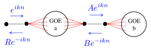
Figure 1: Connectivity of the Hamiltonian. The two dots on the left-hand side represent states in discrete-basis representation of the entrance channel. The dots between the GOE Hamiltonians define an internal channel between them. The quantities in blue are the wave function amplitudes separated into right-moving and left-moving parts, Eqs. (9)-(12).

In this article we construct a reaction model to test the theory by its predictions for the branching ratio between decays from one set of states or the other. The Hamiltonian for each set will be taken from the Gaussian Orthogonal Ensemble (GOE) W84 ; WM09 ; br81 . The wave function for the channel spaces is usually treated by a formal separation of coordinates to define a set of internal coordinates together with a continuous coordinate governing the propagation in the channel. Here we describe the channels in a discrete-basis formalism al20 . This is quite natural for the dynamics of electrons in lattices, but it is also helpful to construct channels involving complex fragments be19 . The structure of the Hamiltonian is depicted in Fig. 1, with the entrance channel on the left-hand side and the bridge channel located between the two GOE reservoirs. We note that a two-reservoir model with GOE ensembles has been used to study fluctuations of decay widths in unimolecular reactions (see Ref. po90 and citations therein).

II Hamiltonian

The model Hamiltonian is defined as

$${\mathbf{H}}=\left[\begin{matrix}0&t_{1}&0&0&0&0\cr t_{1}&0&{\vec{v}}_{2}^{T}&0&0&0\cr 0&{\vec{v}}_{2}&H^{goe}_{a}-i\Gamma_{a}/2&{\vec{v}}_{3}^{T}&0&0\cr 0&0&\vec{v}_{3}&0&t_{2}&0\cr 0&0&0&t_{2}&0&{\vec{v}}_{4}^{T}\cr 0&0&0&0&\vec{v}_{4}&H^{goe}_{b}-i\Gamma_{b}/2\cr\end{matrix}\right].$$ (2)

The first 2-by-2 subblock applies to nearest-neigbor amplitudes in the discretized entrance-channel wave function. Couplings to other states in the entrance channel will be treated implicitly. The next row and column applies to the wave function in the first reservoir of dimension $N_{a}$. Next comes an internal channel consisting of two coupled sites, followed by the second reservoir of dimension $N_{b}$. The total dimension of $\mathbf{H}$ is thus $2+N_{a}+2+N_{b}$. The parameters $t_{1}$ and $t_{2}$ are hopping matrix elements associated with the channels. The embedded GOE Hamiltonians have two parameters, the number of states in the basis $N_{g}$ and the root-mean-square value $v_{g}$ of the matrix elements. They are computed as WM09 ; br81

$$\langle i|H^{goe}_{g}|j\rangle=r_{ij}v_{g}(1+\delta_{i,j})^{1/2}$$ (3)

where $r_{ij}$ is a random number from a Gaussian distribution of unit dispersion, $\langle r_{ij}^{2}\rangle=1$. The vectors $\vec{v}_{k}$ coupling the channels to the GOE states are defined similarly, $\vec{v}_{k}(i)=r_{i}v_{k}$. Inelastic reactions proceed by decays through the states in the two GOE sets. The decays from the two reservoirs to other channels are controlled by the widths $\Gamma_{a}$ and $\Gamma_{b}$.

The main properties of the GOE spectrum needed in this work are the near-Gaussian distribution of the eigenvector amplitudes and the absence of correlations between them. As seen in Eq. (1), The derived properties depend crucially on the level density. This is given by Wigner’s semicircular distribution, which we write as

$$\rho(E)=\rho_{0}\sqrt{1-(E/E_{m})^{2}}$$ (4)

where

$$\rho_{0}=\frac{N_{g}^{1/2}}{\pi v_{g}}$$ (5)

is the level density at the center of the spectrum and

$$E_{m}=2N_{g}^{1/2}v_{g}$$ (6)

is the half-width of the spectrum.

III Reaction theory

There are many formulations of reaction theory for complex systems th09 ; ch13 ; ka15 ; be17 ; al20 ; da01 . For the specific form of our model Hamiltonian (2) it is straightforward to deal directly with the wave function amplitudes and determine the reaction rates by the associated fluxes. To this end, it is convenient to define an effective Hamiltonian that acts on the wave function amplitudes $\phi_{1},\phi_{2}$ of the entrance channel and the amplitudes $\phi_{3},\phi_{4}$ of the channel bridging the two GOE sets of states. The GOE states enter the effective Hamiltonian via self-energy terms

$$w_{kk^{\prime}}=\vec{v}^{T}_{k}\cdot(E-H_{g}^{goe}+i\Gamma_{g}/2)^{-1}\cdot\vec{v}_{k^{\prime}}.$$ (7)

The effective Hamiltonian and the associated channel wave function satisfy the equation

$$\left[\begin{matrix}w_{22}-E&w_{23}&0\cr w_{23}&w_{33}-E&t_{2}\cr 0&t_{2}&w_{44}-E\cr\end{matrix}\right]\left(\begin{matrix}\phi_{2}\cr\phi_{3}\cr\phi_{4}\cr\end{matrix}\right)=-\left(\begin{matrix}t_{1}\phi_{1}\cr 0\cr 0\cr\end{matrix}\right).$$ (8)

Here the GOE Hamiltonian $H_{a}^{goe}$ goes into the calculation of $w_{22},w_{33}$, and $w_{23}$, while $w_{44}$ is calculated with $H_{b}^{goe}$. Eq. (8) is easily solved for the amplitudes on the left-hand side; details are given in the Appendix A. In the remainder of this article we will set $E=0$. This places the incoming energy at the centers of the GOE spectra.

Following the procedure of Ref. al20 , the channel wave functions are separated into right-going and left-going amplitudes as indicated in Fig. 1,

$$\phi_{1} =1-R$$ (9)

$$\phi_{2} =e^{ik_{1}}-Re^{-ik_{1}}$$ (10)

$$\phi_{3} =A-B$$ (11)

$$\phi_{4} =Ae^{ik_{2}}-Be^{-ik_{2}}.$$ (12)

The momentum index $k_{i}$ depends on $E$ and $t_{i}$ by the relation $k_{i}=\cos^{-1}(E/2t_{i})$; it is $k_{i}=\pi/2$ at $E=0$.

The inelastic cross sections may be expressed by a kinematic factor times the transmission coefficients $T$ from the entrance channel to a set of decay channels. The transmission coefficient into the system as a whole is

$$T=T_{a}+T_{b}=1-|R|^{2}$$ (13)

and the coefficient for the $b$ set alone is

$$T_{b}=|A|^{2}-|B|^{2}.$$ (14)

The detailed formulas for the reflection coefficient $R$ and the bridge amplitudes $A,B$ are given in the Appendix A.

IV Branching ratios

The physical observable we examine in this article is the branching ratio $B_{r}$ between the two sets of exit channels. This may be computed from the reaction amplitudes as

$$B_{r}=\frac{T_{b}}{T_{a}}=\frac{|A|^{2}-|B|^{2}}{1-|R|^{2}-|A|^{2}+|B|^{2}}$$ (15)

or by calculating the fluxes directly. The flux into the system from the entrance channel is given by

$$\Phi_{12}=2t_{1}{\rm Im}(\phi_{1}\phi^{*}_{2})$$ (16)

and the flux into the second reservoir is given by the corresponding expression with $\phi_{3},\phi_{4}$ and $t_{2}$. The branching ratio is thus

$$B_{r}=\frac{\Phi_{34}}{\Phi_{12}-\Phi_{34}}.$$ (17)

In terms of the parameters in the effective Hamiltonian the branching ratio is

$$B_{r}=\frac{t_{2}^{2}|w_{23}|^{2}{\rm Im}(w_{44})}{{\rm Im}(w_{22})|s|^{2}-{\rm Im}(w_{23}^{2}w_{44}s^{*})-t_{2}^{2}|w_{23}|^{2}{\rm Im}(w_{44})},$$ (18)

where

$$s=w_{33}w_{44}-t_{2}^{2}.$$ (19)

Note that Eq. (18) for the branching ratio is independent of the parameters that control the coupling to the entrance channel. The parameter $t_{1}$ does not appear in the formula at all. The coupling parameter $v_{2}$ is implicit in the definitions of $w_{22}$ and $w_{23}$, but the numerator and denominator are both proportional to $v_{2}^{2}$ and cancel out. The independence of entrance channel details is not surprising; the entrance channel populates the states in reservoir $a$, but after that only the internal Hamiltonian affects the decay.

V Mean values of the self-energies

The physics of the Hamiltonian is buried in the four complex numbers $w_{ij}$ in Eq. (8). In this section we derive their average values. We first consider the diagonal ones $w_{kk}$ and then the off-diagonal one $w_{kk^{\prime}}=w_{23}$.

V.1 Statistics of the diagonal $w_{kk}$

In this section we will estimate the self-energies in the effective Hamiltonian by taking a continuum limit over the sum over states in the Green’s function $G(E)=(E-H_{g}^{goe}+i\Gamma_{g}/2)^{-1}$. This Green’s function has been analyzed in much more detail in Ref. de07 for different purposes.

The elements of the Green’s function can be written in the eigenstate representation as

$$G_{ij}=\sum_{\lambda}^{N_{g}}\frac{\phi_{\lambda}(i)\phi_{\lambda}(j)}{E-E_{\lambda}}.$$ (20)

Here $E_{\lambda}$ are the eigenvalues of the GOE Hamiltonian including the imaginary offset $-i\Gamma_{g}/2$, and the $\phi_{\lambda}$ are the corresponding eigenvectors. In general the eigenvectors of a complex matrix are necessarily complex as well, but since the imaginary part of the Hamiltonian is a constant offset we can choose them to be real.

We next replace the sum in Eq. (20) by an integral over the level density. See Appendix B for a list of integrals needed in this section. As a simple example, the Stieltjes transform of Tr$(G)$ in dimensionless form pa72 is given by the integral $I_{1}$ in the appendix,

$$f(z)=I_{1}(z)\equiv\int^{+1}_{-1}dx\frac{\sqrt{1-x^{2}}}{z-x}=-\pi\left(\sqrt{z^{2}-1}-z\right).$$ (21)

The replacement of the sum by an integral is most easily justified by demanding that the width satisfies $\Gamma_{g}\gg\rho_{0}^{-1}$ but we shall see later that this condition can be relaxed for ensemble averages.

The diagonal self-energy $w_{kk}$ can be expressed

$$w_{kk}(E)=\sum_{\lambda}^{N_{g}}\frac{(\vec{v}_{k}\cdot\vec{\phi}_{\lambda})^{2}}{E-E_{\lambda}}.$$ (22)

Fig. 2 shows a sampling of the ensemble for a set of Hamiltonian parameters in a GOE space of dimension $N_{g}=100$ at energy $E=0$. There is

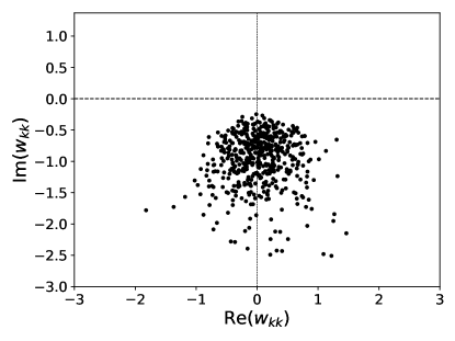
Figure 2: Scatter plot of 500 samples of the $w_{kk}$ ensemble. The Hamiltonian parameters are $N_{g}=100$ and $v_{g},v_{k},\Gamma_{g}=0.1$.

a clustering around a point on the negative imaginary axis, and the spread of values is about the same in the real and imaginary directions. To find the clustering center we examine the ensemble average of Eq. (22),

$$w^{e}_{kk} \equiv\langle w_{kk}(0)\rangle=\left\langle\sum_{\lambda}^{N_{g}}\frac{(\vec{v}_{k}\cdot\vec{\phi}_{\lambda})^{2}}{-E_{\lambda}}\right\rangle$$ (23)

$$=\langle(\vec{v}_{k}\cdot\vec{\phi}_{\lambda})^{2}\rangle\left\langle\sum_{\lambda^{\prime}}^{Ng}\frac{1}{-E_{\lambda}}\right\rangle.$$ (24)

The second line follows from the fact that the eigenvector components are uncorrelated with each other or the eigenenergies. The sum is the same as in the formula for Tr$G$; its ensemble average is

$$\left\langle\sum_{\lambda^{\prime}}^{Ng}\frac{1}{-E_{\lambda}}\right\rangle=-i\rho_{0}I_{1}(z_{g})$$ (25)

with $z_{g}=i\Gamma_{g}/2E_{m}$. The dot products $(\vec{v}_{k}\cdot\vec{\phi}_{\lambda})$ are Gaussian distributed and the variance is easily seen to be

$$\langle(\vec{v}_{k}\cdot\vec{\phi}_{j})^{2}\rangle=v_{k}^{2}.$$ (26)

Bringing these ingredients together, $w_{kk}^{e}$ is given by

$$w^{e}_{kk}=-iv_{k}^{2}\rho_{0}I_{1}(z_{0}).$$ (27)

In physical applications, the widths of the states in the GOE will be much smaller than the overall spread in the GOE, i.e. $|z_{0}|\ll 1$. The corresponding limit in Appendix B yields

$$w^{e}_{kk}\approx-i\pi v_{k}^{2}\rho_{0}\,\,\,{\rm for}\,\,\,\Gamma_{g}\ll E_{m}.$$ (28)

Fig. 3 shows a graph of ${\rm Im}(w_{kk}^{e})$ as function of $\Gamma_{g}$ obtained by Eq. (27) and compared with a value direct sampling of Eq. (22). One sees that the formula is in satisfactory agreement over the entire range examined. This is despite the fact that the fluctuations of the individual samples are small only when $\Gamma_{g}\gg\rho_{0}^{-1}$.

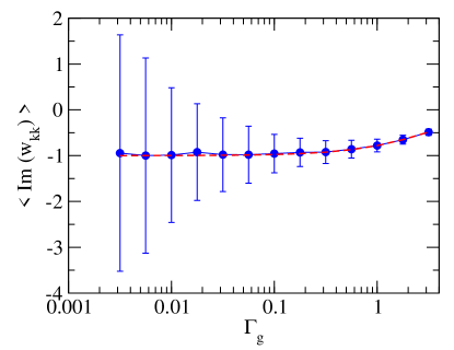
Figure 3: Comparison of Eq. (27) with Eq. (22). The parameters are $N_{g}=100$, $v_{g}=0.1$, and $v_{k}=0.1$. Eq. (22) was evaluated statistically with 500 samples. The means are shown as filled circles, and the error bars denote standard deviation of the samples about the means. The dashed line shows the corresponding value from Eq. (27).

An important consequence of Eq. (28) is that $w_{kk}$ is quite insensitive to the width parameter $\Gamma_{g}$. Since the average reaction observables only depend on the decay width of the second GOE set through $w_{44}$, this proves the insensitivity property. Namely, when the system crosses the transition region it remains in the farther set of states until the final decay into other channels. Eq. (28) can also be easily derived from Fermi’s Golden Rule, as noted in Ref. de07 .

$N_{g}$	Type	sampled	formula	Eq.
100	$w_{kk}$	$-(0.02\pm 0.48)-(1.02\pm 0.47)i$	$-i$	(28)
	$w_{kk^{\prime}}$	$(0.03\pm 0.32)+(0.06\pm 0.35)i$	0
	$|w_{kk^{\prime}}|^{2}$	$0.23\pm 0.27$	$0.2$	(34)
	$w_{kk^{\prime}}^{2}$	$(-0.03\pm 0.21)+(0.02\pm 0.27)i$	$-0.005$	(35)
400	$w_{kk}$	$-(0.00025\pm 0.61)-(1.95\pm 0.55)i$	$-2i$	(28)
	$w_{kk^{\prime}}$	$(-0.014\pm 0.44)+(0.0063\pm 0.47)i$	0
	$|w_{kk^{\prime}}|^{2}$	$0.41\pm 0.41$	$0.4$	(34)
	$w_{kk^{\prime}}^{2}$	$(-0.031\pm 0.44)+(0.045\pm 0.38)i$	$-0.005$	(35)

Table 1: Expectation values and statistical fluctuations of self-energies associated with the coupling of channels to GOE ensembles with the dimension $N_{g}$. The energy parameters $v_{g},v_{k},v_{k^{\prime}},\Gamma_{g}$ are set to 0.1. The sampled results in the third column are the mean values and rms fluctuations obtained from 100 independent samples.

V.2 Statistics of the off-diagonal $w_{kk^{\prime}}$

The mean value of the off-diagonal $w_{kk^{\prime}}$ is zero since the external coupling vectors $\vec{v}_{k}$ and $\vec{v}_{k^{\prime}}$ are independent. However, the branching ratio in Eq. (18) requires only the squared quantities $w_{kk^{\prime}}^{2}$ and $|w_{kk^{\prime}}|^{2}$. To determine the expectation values of these quantities, we first express them in term of the eigenvalues and eigenfunctions of $H_{g}^{goe}-i\Gamma_{g}/2$. The expression for $|w_{kk^{\prime}}|^{2}$ is

$$|w_{kk^{\prime}}(E)|^{2}=\sum_{\lambda,\lambda^{\prime}}^{N_{g}}\frac{u_{kk^{\prime}}(\lambda)u_{kk^{\prime}}(\lambda^{\prime})}{(E-E_{\lambda})(E-E_{\lambda^{\prime}}^{*})}$$ (29)

where $u_{kk^{\prime}}(\lambda)=(\vec{v}_{k}\cdot\vec{\phi}_{\lambda})(\vec{v}_{k^{\prime}}\cdot\vec{\phi}_{\lambda})$. As before, we expose the statistical properties of the dot products by writing them as

$$\vec{v}_{k}\cdot\vec{\phi}_{\lambda}=v_{k}\,r,$$ (30)

where $r$ again is a Gaussian variable with variance $\langle r^{2}\rangle=1$. Thus we can write $u_{kk^{\prime}}(\lambda)=v_{k}v_{k^{\prime}}rr^{\prime}$ where $r$ and $r^{\prime}$ are independent. The double sum in Eq. (29) reduces to a single sum because the $u$’s for different $\lambda$’s are uncorrelated. The numerator in the reduced sum is given by

$$u_{kk^{\prime}}(\lambda)^{2}=v_{k}^{2}v_{k^{\prime}}^{2}r^{2}r^{\prime 2},$$ (31)

which has an expectation value

$$\langle u_{kk^{\prime}}(\lambda)^{2}\rangle=v_{k}^{2}v_{k^{\prime}}^{2}.$$ (32)

The remaining task is to do the sum over $\lambda$, which we again approximate as an integral. Setting $E=0$, the expectation value of $|w_{kk^{\prime}}|^{2}$ becomes

$$\langle|w_{kk^{\prime}}(0)|^{2}\rangle =v_{k}^{2}v_{k^{\prime}}^{2}\frac{\rho_{0}}{E_{m}}I_{3}(c)$$ (33)

$$\approx 2\pi v_{k}^{2}v_{k^{\prime}}^{2}\frac{\rho_{0}}{\Gamma_{g}}$$ (34)

where $I_{3}$ is the integral in Eq.(B3) and its argument is $c=\Gamma_{g}/2E_{m}$. In the last line the integral has been evaluated approximately for $c\ll 1$. Fig. 4 shows $\langle|w_{kk^{\prime}}(0)|^{2}\rangle$ from direct sampling of Eq. (22). The agreement with Eq. (34) is remarkable.

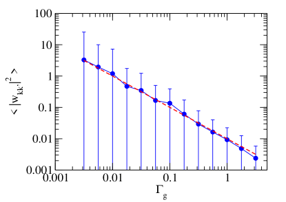
Figure 4: The self-energy term $\langle|w_{kk^{\prime}}|^{2}\rangle$ comparing the formula Eq. (34) with the mean value evaluated with 500 samples from the Hamiltonian ensemble. The mean is shown with filled circles. The errors denote the r.m.s. deviation of the samples about the mean. The dashed line shows the corresponding value from Eq. (34).

The statistical properties of $|w_{kk^{\prime}}|^{2}$ for some numerical examples are shown in Table I (third row in each subtable). One can see that the mean values satisfy Eq. (34) fairly well, even though there is a large fluctuation.

The expectation value of $w_{kk^{\prime}}^{2}$ can be evaluated in a similar way with the integral $I_{2}$ in Appendix B. In the physically interesting region ($c\ll 1$) it becomes

$$\langle w_{kk^{\prime}}^{2}\rangle\approx-\pi v_{2}^{2}v_{3}^{2}\frac{\rho_{0}}{E_{m}}.$$ (35)

This is smaller than $|w_{23}|^{2}$ by a factor of $\Gamma_{g}/2E_{m}$ and can be ignored in deriving the transition-state limit below.

VI Transition-state limit

The transition-state formula Eq. (1) as applied to a single channel can now be derived from Eq. (18) under certain conditions. We neglect the second and third terms in the denominator in Eq. (18) and write

$$B_{r}\approx\frac{t_{2}^{2}|w_{23}|^{2}{\rm Im}(w_{44})}{{\rm Im}(w_{22})|w_{33}w_{44}-t_{2}^{2}|^{2}}.$$ (36)

Next, we define an average value $\overline{B}_{r}$ by replacing the fluctuating quantities in the above equation by their expectation values. This is an approximation because it neglects correlations between them. The result is

$$B_{r} \approx \frac{1}{2\pi\rho_{0}\Gamma_{a}}\frac{4N_{a}t_{2}^{2}v_{a}^{2}v_{3}^{2}v_{4}^{2}}{|v_{3}^{3}v_{4}^{2}N_{a}+t_{2}^{2}v_{a}^{2}|^{2}}$$ (37)

$$= \left(\frac{1}{2\pi\rho_{0}\Gamma_{a}}\right)\left(\,\frac{-4t_{2}^{2}w_{33}w_{44}}{|-w_{33}w_{44}+t_{2}^{2}|^{2}}\right).$$ (38)

The first term in parentheses is exactly the transition-state branching ratio for $T=1$. The second term in parentheses can be interpreted as the transmission factor $T_{ab}$ between the two reservoirs. The full derivation is given in Appendix C. It is easy to show that it is equal to one if the transmission factors between the bridge channel and the two reservoirs are both unity, as may be seen by the following arguments. The transmission factor between the bridge channel and reservoir $b$ is

$$T_{cb}=(|A|^{2}-|B|^{2})/|A|^{2}$$ (39)

which reaches one when $|B|^{2}=0$. According to Eq. (49), this is achieved if $w_{44}=-it_{2}$. A similar condition applies to the transmission coefficient to the first reservoir, $w_{33}=-it_{2}$. Imposing both conditions, the second factor in Eq.(38) reduces to unity.

We have also evaluated the transition state formula numerically, sampling the ensemble with Eq. (18). Taking the example with all $v$’s and $\Gamma$’s equal to 0.1 and $t_{1}=t_{2}=-1$, the self-energies satisfy the condition that $T_{ca}=1$ and $T_{cb}=1$. We obtain

$$B_{r}=0.048\pm 0.048\,\,\,{\rm(numerical)}$$ (40)

by sampling the Hamiltonian ensemble.

This is to be compared with the analytic formula which gives

$$\overline{B}_{r}=0.048\,\,\,{\rm(analytic)}.$$ (41)

The agreement here is somewhat unexpected, considering the fact that the averaged internal transmission factor can only be smaller than one. This may be seen in Fig. 5 showing $T_{cb}$ as a function of $E$ for the same Hamiltonian as before.

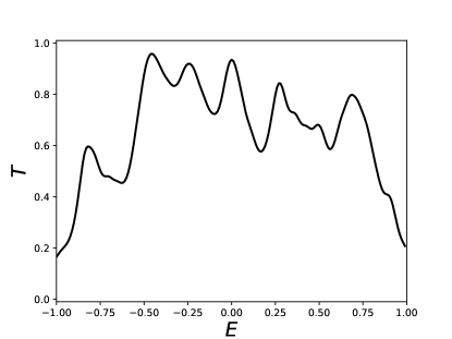
Figure 5: Transmission coefficient from a channel into a representative GOE sample. The GOE Hamiltonian parameters are the same as in Fig. 2 and $t=-1$ in the channel Hamiltonian.

VII Summary and Discussion

The model described in Section II treats reactions involving a quantum system that can decay in two distinct ways, one through states directly coupled to the entrance channel and the other through a second set of states coupled to the first via an internal channel (often called a “transition state”). The states in both sets are chaotically mixed as given by the well-known Gaussian orthogonal ensemble. The statistical properties of the model can be analyzed to a large extent analytically, permitting a qualified derivation of the transition-state theory encapsulated in Eq. (1). Two of our findings appear to be quite robust:

1) The branching ratio between the decay modes is independent of the details of the coupling to the entrance channel. This is important if the reaction proceeds through isolated resonances visible from the entrance channel—one does not have to deal with specific energies of physical resonances to calculate average properties.

2) The transition-state formula does not require knowledge of the decay widths of states in the second set, and this insensitivity is verified over a large range of Hamiltonian parameters. In other words, once the flux has passed over the barrier, it does not matter how long it takes to decay from the states on the other side. The only caveat is that the width should not be larger than the full spread of the GOE spectrum.

Our derivation of the transition-state theory provides a formula for the transmission coefficient in terms of the parameters in the Hamiltonian ensemble. A related finding is:

3) Systems having a transmission factor $T=1$ should be a rare occurrence, since it demands a specific coupling strength of the bridge channel to both sets of GOE states. Furthermore, the coupling $t_{2}$ within the channel has to be much larger than the other interactions in the Hamiltonian. This requires some additional physics: in chemistry this is provided by the kinetics of nuclear motion. In Fermi systems it might be provided by a superfluidity from a pairing interaction.

For a possible future application of the methods discussed here, one could consider two chaotic sets of states coupled through a single state instead of a channel. The expected transmission coefficient is given by the quantum-dot formula (al00, , Eq. (21)),

$$T_{ab}=\frac{\Gamma_{a}\Gamma_{b}}{(E-E_{r})^{2}+(\Gamma_{a}+\Gamma_{b})^{2}/4}.$$ (42)

Here $E_{r}$ is the diagonal energy of the bridge state; $\Gamma_{a},\Gamma_{b}$ correspond to ${\rm Im}(w_{33}),{\rm Im}(w_{44})$ in our notation.

Some caveats in our analysis should be repeated. First, our derivations of analytic formulas are valid only for $\Gamma\gg\rho_{0}$, corresponding to the overlapping resonance limit in the two sets of states. However, the statistical properties of the self-energies and other derived quantities such as ratio formula Eq. (18) appears to be valid also when the resonances are isolated. It would be interesting to see if the derivations could be extended to cover such cases as well. Second, we have ignored fluctuations in the spectral function in calculating the statistical properties of the GOE Green’s function. This may well be justified by Dyson’s spectral rigidity, but our methodology is not adequate to address that approximation.

In this paper we have concentrated on the mean values of the self-energies and the branching ratios. We will discuss their fluctuations, in particular, the validity of the Porter-Thomas distribution, in a separate publication bh2021-2 .

Appendix A Reflection coefficient and the bridge amplitudes

The wave function amplitudes $\phi_{2},~{}\phi_{3}$, and $\phi_{4}$ obtained by inverting the matrix in Eq. (8) are

$$\phi_{2} =-(w_{33}w_{44}-t_{2}^{2})t_{1}\phi_{1}/D$$ (43)

$$\phi_{3} =w_{23}w_{44}t_{1}\phi_{1}/D$$ (44)

$$\phi_{4} =-w_{23}t_{2}t_{1}\phi_{1}/D$$ (45)

where

$$D=w_{22}w_{33}w_{44}-w_{22}t_{2}^{2}-w_{23}^{2}w_{44}.$$ (46)

These expressions are inserted into Eq. (9-12) and solved for the transport amplitudes $R,A,$ and $B$. The result at $E=0$ is

$$R =\frac{(w_{33}w_{44}-t_{2}^{2})t_{1}+iD}{(w_{33}w_{44}-t_{2}^{2})t_{1}-iD}$$ (47)

$$A =-\frac{t_{1}w_{23}}{2iD}(1-R)(t_{2}-iw_{44})$$ (48)

$$B =-\frac{t_{1}w_{23}}{2iD}(1-R)(t_{2}+iw_{44}).$$ (49)

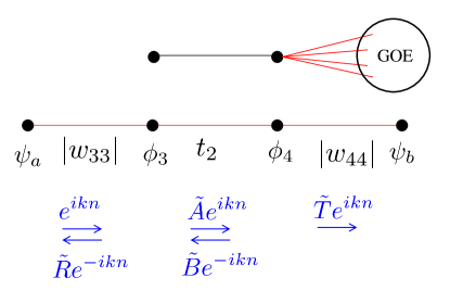
Figure 6: The chain of four states shows channels and the wave function amplitudes in the discrete-basis representation needed to evaluate the transmission factor $T_{ab}$. The partial transmission factors $T_{ca}$ and $T_{cb}$ are set by the properties of the Hamiltonian consisting of a channel with a single GOE reservoir, shown at the top.

Appendix B Self-energy integrals

The statistical properties of the self-energy are calculated making use of the following integrals:

$$I_{1}(z)=\int^{+1}_{-1}dx\frac{\sqrt{1-x^{2}}}{z-x}=\pi\left(z-\sqrt{z^{2}-1}\right)$$ (50)

$$I_{2}(z)=\int_{-1}^{+1}dx\frac{\sqrt{(1-x^{2})}}{(z-x)^{2}}=\pi\left(\frac{z}{(z^{2}-1)^{1/2}}-1\right)$$ (51)

$$I_{3}(y)=\int_{-1}^{+1}dx\frac{(1-x^{2})^{1/2}}{(x^{2}+y^{2})}=\frac{\pi}{y}\left(\sqrt{1+y^{2}}-y\right)$$ (52)

$$I_{4}(y)=\int_{-1}^{+1}dx\frac{(1-x^{2})^{1/2}}{(x^{2}+y^{2})^{2}}=\frac{\pi}{2y^{3}\sqrt{1+y^{2}}}.$$ (53)

The first integral is the Stieltjes transform of the semicircular GOE level density in dimensionless form as discussed by Pastur pa72 . The integral $I_{2}$ can be derived from it by differentiation. The integrals $I_{3}$ and $I_{3}$ have been checked by numerical integration.

We especially require the leading behavior of the integrals for small positive imaginary $z$ and small real $y$. In those limits the integrals become

$$I_{1}(z)\approx-i\pi$$ (54)

$$I_{2}(z)\approx-\pi$$ (55)

$$I_{3}(y)\approx\frac{\pi}{y}$$ (56)

$$I_{4}(y)\approx\frac{\pi}{2y^{3}}.$$ (57)

Appendix C Transmission factor

Under certain conditions, the second factor in Eq. (38) reduces to the transmission factor $T_{ab}$ between the two reservoirs. To derive $T_{ab}$ from the Hamiltonian parameters we need to know the transmission and reflection amplitudes at the interface between the bridge channel and both reservoirs. The reflection probability at the interface between the bridge channel and the second reservoir is readily available as the ratio

$$R=B/A=\frac{t_{2}+iw_{44}}{t_{2}-iw_{44}}.$$ (58)

Taking $w_{44}$ to be negative imaginary as in Eq. (28), one can show that the reflection amplitude would be the same for an interface to another channel consisting of a chain of states connected by nearest-neighbor interactions of magnitude $t_{b}={\rm Im}(w^{e}_{44})$ The same argument applies to the interface with the first reservoir, where the magnitude of the coupling in the fictitious channel is $t_{a}={\rm Im}(w^{e}_{33})$.

The surrogate Hamiltonian is depicted as the middle chain of four states in Fig. 6. The two bridge states in the middle are connected to the closest states in each channel. The Hamiltonian equation for amplitudes $\phi_{3}$ and $\phi_{4}$ are given by

$$|w_{33}|\psi_{a}+t_{2}\phi_{4}=E\phi_{3}=0,$$ (59)

$$t_{2}\phi_{3}+|w_{44}|\psi_{b}=E\phi_{4}=0,$$ (60)

for scattering at $E=0$. The amplitudes on the four sites are expressed in terms of the traveling wave amplitudes $\tilde{R},\tilde{A},\tilde{B}$ and $\tilde{T}$ as shown in the figure. The phase of these amplitudes change by $e^{\pm ik}$ from one site to the next in a channel. These lead to the equations for the amplitudes

$$\psi_{a} = e^{-3ik/2}-\tilde{R}e^{3ik/2},$$ (61)

$$\phi_{3} = e^{-ik/2}-\tilde{R}e^{ik/2}=\tilde{A}e^{-ik/2}+\tilde{B}e^{ik/2},$$ (62)

$$\phi_{4} = \tilde{A}e^{ik/2}+\tilde{B}e^{-ik/2}=\tilde{T}e^{ik/2},$$ (63)

$$\psi_{b} = \tilde{T}e^{3ik/2}.$$ (64)

Substituting these wave functions into Eqs. (59) and (60) with $k=\pi/2$ for $E=0$, one finds that the coefficient of the travelling wave in channel $b$ is

$$\tilde{T}=\frac{2t_{2}|w_{33}|}{||w_{33}w_{44}|+t_{2}^{2}|^{2}}.$$ (65)

Since the incoming flux and the outgoing flux are proportional to $|w_{33}|$ and $|w_{44}||\tilde{T}|^{2}$, respectively, the transmission factor from the left reservoir to the right is

$$T_{ab}=\left|\frac{w_{44}}{w_{33}}\right|\,|\tilde{T}|^{2}=\frac{4t_{2}^{2}|w_{33}w_{44}|}{||w_{33}w_{44}|+t_{2}^{2}|^{2}}.$$ (66)

Noticing $|w_{33}w_{44}|=-w_{33}w_{44}$, this coincides with the second fractional factor in Eq. (38).

References

- (1) N. Bohr and J.A. Wheeler, Phys. Rev. 56, 426 (1939).
- (2) D.G. Truhalar, B.C. Garrett, and S.J. Klippenstein, J. Phys. Chem. 100, 12771 (1996).
- (3) D.G. Truhalar, W.L. Hase and J.T. Hynes, J. Phys. Chem. 87, 2664 (1983).
- (4) G. Mills and H. Jónsson, Phys. Rev. Lett. 72, 1124 (1994).
- (5) W.H. Miller, J. Chem. Phys. 61, 1823 (1974).
- (6) K.J. Laidler and M.C. King, J. Phys. Chem. 87, 2657 (1983).
- (7) R.A. Marcus and O.K. Rice, J. Phys. and Colloid Chem. 55, 894 (1951).
- (8) R.A. Marcus, J. Chem. Phys. 20, 359 (1952).
- (9) C.E. Porter and R.G. Thomas, Phys. Rev. 104 , 483 (1956).
- (10) H.A. Weidenmüller, Ann of Phys. (N.Y.) 158, 120 (1984).
- (11) H.A. Weidenmüller and G.E. Mitchell, Rev. Mod. Phys. 81, 539 (2009).
- (12) T.A. Brody, et al., Rev. Mod. Phys. 53, 385 (1981).
- (13) Y. Alhassid, G.F. Bertsch, and P. Fanto, Ann. Phys. (N.Y.) 419, 168233 (2020).
- (14) G.F. Bertsch and W. Younes, Ann. Phys. 403, 68 (2019).
- (15) W.F. Polik, et al., J. Chem. Phys. 92, 3471 (1990).
- (16) I.J. Thompson and F.M. Nunes, Nuclear Reactions for Astrophysics (Cambridge University Press, Cambridge, 2009).
- (17) L. F. Canto and M. S. Hussein, Scattering Theory of Molecules, Atoms and Nuclei (World Scientific, Singapore, 2013).
- (18) T. Kawano, P. Talou, and H.A. Weidenmüller, Phys. Rev. C 92, 044617 (2015).
- (19) G.F. Bertsch and T. Kawano, Phys. Rev. Lett. 119, 222504 (2017).
- (20) P.S. Damle, A.W. Ghosh, and S. Datta, Phys. Rev. B 64, 201403, (2001).
- (21) A. De Pace, A. Molinari and H.A. Weidenmüller, Ann. of Phys. 322, 2446 (2007).
- (22) L.A. Pastur, Theoretical and Mathematical Physics 10, 74 (1972).
- (23) Y. Alhassid, Rev. Mod. Phys. 72, 895 (2000).
- (24) G.F. Bertsch and K. Hagino, to be published.